ISLAMIC UNIVERSITY OF GAZA DEANERY OF HIGHER STUDIES FACULTY OF SCIENCE DEPARTMENT OF MATHEMATICS

Solitary Waves in Lossy Linear and Lossless Nonlinear Metamaterials

Waveguide Structure

Presented by

Asmahan Rafiq Muhsen

Supervised by

Prof. Dr. Mohammed M. Shabat

A THESIS Submitted to the Faculty of Science as a Partial Fulfillment of the

Master of Science in (M. Sc.) in Mathematics

January -2015

] يتما أوتمي وبر رأم نم وحوح قل الرن الرع ألونكسيو

]من العلم إلا قليلا]85:اإلسراء[

I

DEDICATION

§ To my beloved parents.

§ To my devoted husband.

§ To my sister and brother.

§ To my children.

§ To my friends.

II

ACKNOWLEDGEMENT

§ Thanks to God almighty for the completion of this study. Only due to

his blessings I could finish it.

§ I would like to express my deepest gratitude to my advisor, Professor

Dr. M. M. Shabat, for his patience, invaluable advises and

suggestions. Without him, it would be impossible to finish this study.

§ I would like also to thank Dr. Zeyad Al-sahhar from department of

physics at Al-Aqsa University for fruitful discussion , important

suggestions.

§ My thanks also go to members of Mathematics department at the

Islamic University of Gaza.

§ I would like to thank my beloved parents, husband and family for

their encouragement who are supportive to me throughout my life.

III

CONTENTS

DEDICATION……………………………………………….. I

ACKNOWLEDGEMENT…………………………………. II

CONTENTS………………………………………………… III

ABSTRACT………………………………………………… VI

VII …...………………………………………………ملخص البحث

List of Figure Captions ……………………………………… VIII

Preface ……………………………………………………… IX

CHAPTER ONE Introduction

1.1 Plannar Waveguides……………………………………… 1

1.2 Electromagnetic waves………………………………… 3

1.2.1 TE waves……………………………………………… 3

1.2.2 TM waves……………………………………………… 4

1.3 Metamaterials…………………………………………… 5

1.4 The refractive index n ………………………………….. 6

1.5 Maxwell's equation……………….…………………… 7

1.5.1 Linear wave equation………………………………… 9

1.5.2 Non-linear wave equation …………………………… 9

1.6 Boundary Conditions for electromagnetic field……… 10

1.7 Solitary Waves…………………………………………… 11

IV

CHAPTER TWO Preliminaries

2.1 Weierstrass elliptic function…………………………… 13

2.1.1 Definition of Weierstrass elliptic function…………... 13

2.1.2 Integral representation of ( )z℘ 14

2.1.3 Properties of Weierstrass function………………….. 15

2.1.4 The addition theorem for the function ( )z℘ ………… 16

2.1.5 Descriptive properties of Weierstrass function……… 17

CHAPTER THREE Existence of Eigen Waves and Solitary Waves in Lossy Linear

Introduction …………………..…………………..………… 19

3.1 Geometry of the problem ……………………………… 19

3.2 Solutions to differential equation if ( )1

_

1ε = ε 1+iα 20

3.3 Solution of the differential quation in the nonlinear film cast 27

3.4 Conclusion …………………………………………… 30

CHAPTER FOUR TE- Polarized Guided by a Lossless Nonlinear

Three – layer Structure

4.1 Introduction …………………………………………… 31

4.2 Real, Nonnegative and bounded field intensities ……. 33

4.3 Solutions of the dispersion relation …………………… 42

V

4.4 Guided waves in a structure with linear substrate and film and nonlinear cladding. ……………………………………..

50

4.5 Conclusion ………………………………………………. 54

CHAPTER FIVE TE - Guided Waves in a three Layer Structure with

Kerr – type Nonlinearity

5.1 Introduction …………………………………………… 55

5.2 Formulation……………………………………………… 55

5.3 Convergence of iteration …..…………………………… 59

5.3.1 Linear case …..………………………………………… 59

5.3.2 Nonlinear case ………………………………………… 62

5.4 Existence ………………………………………………… 67

5.5 Conclusion …….………………………………………… 70

References …………………………………………………… 71

VI

ABSTRACT

Metamaterials have entered into the main stream of electromagnetics due to their

unusual and desired qualities, so propagation of electromagnetic waves in

metmaterials has been intensively studied over last two decades, specially

Solitary waves which has received an increasing attention for researchers in

many different fields.

Planner waveguides formed by one or several layers has attracted considerable

attention, so in this work we consider TE- electromagnetic waves propagating in

planner waveguide formed by three-layers, with the waveguide is filled either by

linear medium or nonlinear medium with nonlinearity described by the kerr-law

Modern mathematical methods for investigating the polarized electromagnetic

wave propagation in nonlinear waveguide structure are considered to solve

Maxwell equation in linear, nonlinear planner waveguide when the permittivity is

constant and when it is a function of field intensity. In each case we derive the

dispersion relation.

VII

البحث ملخص

، وتتمیز بأن السماحیة - صناعیة- (مواد ال توجد في الطبیعة لقد دخلت المواد فوق العادة

في التیار الرئیسي للكهرومغناطیسیة بسبب الكهربائیة والنفاذیة الكهرومغناطیسیة لها قیم سالبة)

موضوع انتشار الموجات الكهرومغناطیسیة في وسط حظيصفاتها المرغوبة وغیر الطبیعیة ولذلك

الباحثین على مر السنوات السابقة، خاصة الموجات المنعزلة الكثیر من اهتمام بللمواد فوق العادة

تى ومختلف المجاالت.التي تلقت الكثیر من انتباه الباحثین في ش

موجة كهرومغناطیسیة منتشرة في وسط مكون من ثالث شرائح، وهذه TEوفي هذا البحث اعتبرنا

األوساط إما أن یكون فیها مادة خطیة أو غیر خطیة.

ي لكل وسط ومعادلة التشتت ائوباستخدام معادالت ماكسویل تم اشتقاق مركبات المجال الكهرب

أو دالة متصلة أو یعتمد على ا ثابت ا كانت السماحیة الكهربائیة عددللنظام المفروض، سواء

مركبات المجال الكهربائي.

VIII

List of Figur Captions:

Figure 1.1 Parallel-plate waveguide with metal plates at x=0,d, between the plates is dielectric of permittivity ε ……………………………….. 1

Figure 1.2 Rectangular waveguide ………………………. 1

Figure 1.3 Cylindrical waveguide ………………………… 2

Figure 1.4 Symmetric Slab waveguide with slab region … 2

Figure 1.5 Optical fiber waveguide with the core (r<a) and the cladding (a<r<b) …………………………..

2

Figure 1.6 Diagram of the three layer planner waveguide structure ……………….................……………

2

Figure 1.7 Electromagnetic wave propagating in the positive X direction …………………………….

3

Figure 1.8 Negative refractive index metamaterial……….. 6

Figure 1.9 Soliton …………………………………………. 11

Figure 2.1 FPP of Weierstrass elliptic function …………... 18

Figure 3.1 Geometry of the Problem of Chapter 3 ……….. 20

Figure 4.1 FPP for positive and negative Discriminants .f∆

\

\

pp

=ε denotes the normalized derivative of

Weierstrass's functions P(u) …………………… 50

IX

Preface

Problems of electromagnetic waves propagation in linear and nonlinear waveguide structure are intensively investigated during several decades [1, 2, 3, 4, 5]. Propagation of electromagnetic wave in layers and cylindrical waveguides are among such problems. Phenomena of electromagnetic wave propagation in nonlinear media have original importance, and also find a lot of application, for example, in plasma physic, microelectronics optics, laser technology [6, 1, 2]. Specially solitary waves are the localized waves which propagate without change of its properties (shape, velocity, etc). These waves have been the subject of intense theoretical and experimental studies in many different fields, including hydrodynamics nonlinear optics, and biology.

By using permittivity and permeability mediums can be classified to four categories. Metamaterials are one of these categories which have both negative permittivity and permeability, so they are not available in nature, they are engineered to provide properties not available in nature, and so they gain their properties from structure rather than composition. So problems of such wave propagation in a linear metamaterial were deeply studied many years ago, for example [3]. Such problems are formulated as boundary eigenvalue problems for ordinary differential equations.

In our work, we will study the solitary waves in some waveguide structure containing lossy linear and lossless nonlinear metamaterials.

Let us give a survey of the thesis:

In chapter 1 we introduce some physical definitions that will be dealt with along the thesis, we introduce the planner waveguide, electromagnetic wave, metamaterials, and we derive the differential equation needed from Maxwell's equation in both nonlinear media and finally we introduce solitary waves.

In chapter 2 we introduce an important function, Weierstrass elliptic function and some important properties of ( )z℘ .

In chapter 3 we consider TE wave propagation in a three – layer waveguide in where the three layers are linear. The dispersion relation is derived and analyzed,

X

and we consider TE electromagnetic with nonlinear film and a solitary–like solution is derived.

In chapter 4, we consider TE wave propagation in planner waveguide with three–layer structure in which all media in the layers have arbitrary nonlinearity. The permittivity in the layer is an arbitrary function with respect to electric field intensity. We derive dispersion relation. Also the condition for real, nonnegative and bounded electric field intensity are obtained.

In chapter 5 we consider TE wave propagation in three–layer waveguide in which the film is fulfill with media in which permittivity ε , which is a real – valued function, and we derive a series solution, and prove the convergence of this series.

1

CHAPTER 1

Introduction This chapter deals with the fundamental concepts of physical definitions needed throughout this thesis, it presents waveguide, electromagnetic waves, metamaterials, solitary waves, and finally we derive the basic linear and nonlinear equation from Maxwell's equation required to carry out this work.

1.1 Planar Waveguides

Waveguide are essential parts of millimeter and submillimeter-wave devices and system. They are used for guiding electromagnetic energy between the components of the system. So waveguide is a structure through which electromagnetic waves can be transmitted from point to point, and within the fields are confined to a certain extent [1].

Planner waveguides consists of a longitudinally extended high – index optical medium, called the core which is transversely surrounded by low– index called the cladding. So waveguides are the most efficient way to transfer electromagnetic energy. Waveguide are essentially coaxial lines without center conductors. They are constructed from conductive material.

Waveguides assume many different forms that depend on the purpose of the guide, and the frequency of the waves to be transmitted. The simplest form is the parallel plate guide shown in Fig (1.1). Other forms are the hollow-pipe guide, , including the rectangular waveguide of Fig (1.2), and the cylindrical guide, shown in Fig (1.3). Dielectric waveguides, used primarily at optical frequencies, include the slab waveguide of Fig (1.4) and the optical fiber, shown in Fig (1.5). Each of these structures possesses certain advantages over the others, depending on the application and the frequency of the waves to be transmitted All guides – however exhibit the same operating principle [1] .

Fig (1.1):Parallel-plate waveguide with metal plates at x=0,d between the plates is a diclectric of permittivity

Fig (1.2): Rectangular waveguide

2

Fig (1.3): Cylindrical Waveguide

Fig(1.4): Symmetric Slab Waveguide with Slab region

Fig (1.5): Optical fiber waveguide, with the core (r < a) and the cladding

(a < r < b)

A planar waveguide is characterized by parallel planar boundaries with respect to one (x) direction, but is infinite in extent in the lateral direction (z and y). In this thesis we will consider the simple three-layer planar waveguide structure of Fig (1.6). The layers are all assumed to be infinite in extent in the y and z directions, and layers 1 and 3 are also assumed to be semi-infinite in the x-direction. [7]

For planner waveguide, the modes are either TE or TM which will be discussed in section (1.2).

Furthermore, we consider 0=∂∂y

because the index profile is independent of the

y – direction.

Fig (1.6): Diagram of the three-layer planar waveguide structure.

3

1.2 Electromagnetic waves

During the early stages of studies of electric and magnetic phenomena, electric and magnetic fields were thought to be unrelated. In 1865 James Clark Maxwell provided a mathematical theory that showed a close relation between electric and magnetic phenomena.

Later Hertz provided that the electric and magnetic fields are related when he generate and detect the electromagnetic waves in a laboratory experiment. So an electromagnetic wave consists of mutually perpendicular and oscillating electric and magnetic fields which are perpendicular to the direction in which the waves travel (propagate) So the electromagnetic wave is transverse wave.

Also the propagation of electromagnetics is governed by the Maxwell's equations which will be explained later in section (1.5). Regardless of their frequency electromagnetic waves do not require a medium to propagate , they can not only travel through solid materials but also travel through vacuum, at the same speed of light C (c=3.00 ×108 m/s). Electric field and magnetic field's strength of an electromagnetic wave vanishes as z→∞. [8]

Electromagnetic waves are classified into several different types, but they are all part of a single continuous spectrum. There are radio waves which have wavelength of the order 102 meters, microwaves with wavelength of the order 10-2 m, infra red 10-5m, optical waves 10-7m, and X-rays 10-10m.

Fig (1.7): Electromagnetic wave propagating in the positive X direction

Any electromagnetic wave can be expressed as a lin'ear combination of TE, and TM waves.

1.2.1 TE waves

In this case the electric intensity Er

is parallel to the interface. It is pointing in the y–direction corresponds to the perpendicular to the plane of incidence. (s– polarized).

So the electric field vector is entirely in the y–plane direction but it has no component of H in this direction because the magnetic field strength H is

4

entirely transversed. Thus Hr

has components only in x and z directions (i.e.) we can write,

( )0 , , 0 ,yE E=r

( ), , .x zH H H=r

0

1.2.2 TM waves

In this case, the magnetic field vector Hr

is parallel to the interface, TM mode results a p-polarized wave, that is the entire H

r field is entirely in the y– direction

but not of the electric field, So we can write,

( )zx EEE ,0,=r

( ), ,yH H= 0 0r

Definition 1.1:

• A homogenous medium is one for which the quantities: permittivity ε , permeability µ , and conductivity σ are constants through the medium.

• The medium is isotropic if ε is a scalar constant so that D and E have everywhere the same direction.

Now, it is well known that the response of a system to the presence of an electromagnetic field is determined to a large extent by the electrical properties of the materials involved, these macroscopic parameters are the permittivity ε, permeability µ, and conductivity σ [2]. A medium with both permittivity and permeability greater than zero (ε > 0, µ > 0) are called double positive medium most occurring media or regular materials. A medium with permittivity ε < 0 and permeability µ > 0 are called Epsilon negative (ENG) medium. In certain frequency regimes many plasmas exhibit this characteristics. A medium with permittivity ε > 0 and permeability µ < 0 are called Mu negative (MNG) medium. Some gyrotropic materials exhibit this characteristic in certain frequency regimes. They also include ferromagnetic or antiferromagnetic systems. Finally a medium with both negative permittivity and permeability (ε < 0, µ < 0) are called as Double negative (DNG) medium [9, 10].

These materials with negative refractive index are not known to occur in nature. However the phenomenon does occur in specially designed materials called metamaterials.

5

1.3 Metamaterials

Metamaterials have become a new subdiscipline within physics and electromagnetism (specially optics and phonetics) [9], Metamaterials are artificially structured materials featuring properties that do not or may normally take place and can not be acquired in nature [9, 11]. This new type of materials with the negative index refraction were theoretically investigated in 1967 by veslago who investigated plane – wave propagation in material whose permittivity and permeability wave assumed to be simultaneously negative. His theoretical study show that for a mono chromatic uniform plane – wave in such a medium the direction of the pointing vector is antiparallel to the direction of the phase velocity, contrary to the case of plane – wave propagation in conventional simple media. In recent years, Smith, Schultz and their group constructed such a composite medium for the microwave regime and demonstrated experimentally the presence of anomalous refraction in this medium [2]. In recent years greater attention has been paid to the metamaterials which have uncommon electromagnetic properties. These materials usually gain these physical properties from structure rather than composition. So the essential property in metamaterials is their usual and desired qualities that appear due to their particular design and structure [9].

The unconventional response functions of metamaterials are often generated by artificially fabricated inclusions or inhomogeneities embedded in a host medium or connected or embedded in a host surface [2].

These unusual properties of negative refractive index material reveal themselves most prominently when the refractive index of the same medium can be positive in one spectral region and negative in another [12].

Metamaterials have many interesting phenomenon that do not appear in natural media. Among them there are the modification of Snell's law, the Doppler shift reversed meaning that the frequency of a light source moving toward an observer appears to deduce the negative phase velocity time overaged poynting vector is antiparallel to phase velocity, i.e. the wave fronts are moving in the opposite direction to the flow of energy [13] the positive intrinsic impendence and the modified boundary conditions. [14] Gerenkov radiation is electromagnetic radiation emitted within a charge particle passes through a dielectric medium at a speed greater than the phase velocity of light in that medium and reformulation of the Fermat principle [15].

One of the first significant applications of these structures was to manipulate the RF flux in all nuclear magnetic resonance system. Metamaterials are also shown to operate at microwave, millimeter wave, THZ , mid IR, IR and visible regimes of electromagnetic spectrum utilization for metamaterials at the optical regime could lead to high performance and novel phonotics devices in information and communication technologies [10]

6

Fig (1.8): Negative refractive index metamaterial

and they are so important in electromagnetics since metamaterial affects electromagnetic waves by having structural features smaller than the wavelength of electromagnetic radiation it interacts with [7].

1.4 The refractive index n

The refractive index n is a measure of how much speed of a wave is reduced inside the medium relative to the speed in vacuum. It is determined by the permittivity and permeability through

,n εµ=

where µ is relative magnetic permeability and ε relative dielectric permittivity.

The refractive index can also be used to determine the change in the direction of the wave as it passes through a medium interface, that is the refraction index [15]

If we change simultaneously the signs of ε and µ, the ratio n2=µε will not change. If both ε and µ are positive, this means that n = µε . If ε and µ are negative in a given wavelength range, this means that n = - µε [13]. In negative index metamaterials the pynting vector S=[EH] and the vectors E and H form the left hand triple, which leads to opposite directions of the group and phase velocity of plane waves propagating in the materials.

Also we define ok , the wave number of free space, by

ck ω

=o ,

where ω is the angular frequency of the wave and c is the velocity of vacuum.

7

1.5 Maxwell's equation

All the Analysis of electromagnetic waves propagation is based on Maxwell's equations, which govern the time dependence of the intensity of the electric and

magnetic fields →

E and →

H respectively [16]

, ( . )BEt

→ ∂∇× =

∂

uur1 1

, ( . )DHt

→ ∂∇× =

∂

uur1 2

where D is the electric flux density and B is the magnetic flux density.

We can also introduce the electric permittivity ε and the magnetic permeability µ . These two parameters characterize the response of the material to an external electric and magnetic fields as

D E, (1.3)ε→ →

=

H, (1.4)B µ→ →

=

regardless of whether the fields are in a linear or nonlinear medium.

The electric field and magnetic field for the TE waves propagating along the z-axis with angular frequency ω , and waves vector β can be expressed as:

y

x z

i(β t)E (0,E ,0) e ,

i(β t)H (H ,0,H ) e .

z

z

ω

ω

→

→

−=

−= (1.5)

Now, we substitute expressions (1.3) and (1.4) into Eq. (1.1), and (1.2). Then for linear isotropic dielectric waveguide characterized by a spatial permittivity distribution ( )yx,ε the Maxwell's equation can be written as:

, ( . )HEt

µ→

→ ∂∇× =

∂1 6

. ( . )EHt

ε→

→ ∂∇ × =

∂1 7

8

substituting Eq. (1.5) in Eq. (1.6) for TE waves we obtain,

x y z x y z

i j k i j k

E H Hy x z

i µ

∧ ∧ ∧ ∧ ∧ ∧

∂ ∂ ∂ ∂ ∂ ∂=

∂ ∂ ∂ ∂ ∂ ∂

0 0 0

which yields,

( )y

y x z

Ei E i j i H i H j

xβ µω

∧ ∧ ∧ ∧∂+ = +

∂

Then ( . )y x x yi E i H and H E aββ µω

µω= = 1 8

Also ( . )y yz z

E Eii H and H bx x

µωµω

∂ ∂=− =

∂ ∂1 8

Similarly evaluation of Eq.(1.7) yields

. ( . )x zy

H H i Ez x

εω∂ ∂

− = −∂ ∂

1 9

Substituting xHz

∂∂

and zHx

∂∂

from Eq.(1.8) into Eq.(1.9) we write

.y yy

H Ei i Ez x

β εωµω µω

∂ ∂− = −

∂ ∂

2

2 (1.10)

Differentiate the electric field in Eq. (1.5) gives yEi E

zβ

∂=

∂.

Substitute this in Eq.(1.10) we have

yy y

Ei iE i Ex

β εωµω µω

∂− = −

∂

22

2 (1.11)

Multiply by ( )µω we get,

( ) .yy

EE

xβ ω ε µ

∂− − =

∂

22 2

2 0 (1.12)

9

If we substitute rε ε ε= o and rµ µ µ= o where ,ε µo o is the permittivity and permeability at vacuum, and ,r rε µ the relative permittivity and permeability, then Eq. (1.12) becomes

( ) .yr r y

EE

x cω

β ε µ∂

− − =∂

2 22

2 2 0

If we substitute β2 = 2

2 2 20 0 2k n , k

cω

= in Eq. (1.12) we can write

22 202 ( ) 0.y

y

EK n E

xε µ

∂− − =

∂ (1.13)

Modal solution are sinusoidal (-sine wave- is a mathematical curve that describes a smooth repetitive oscillation) or exponential, depending on the sign of

( )2 2k n εµ− ⋅o

1.5.1 Linear wave equation

For the electromagnetic wave propagating in media with a real linear permittivity ,rε

r Lε ε= (1.14)

The Eq. (1.13) for the nonmagnetic layer ( )1=µ , becomes

22 202 ( ) 0y

r y

EK n E

xε

∂− − =

∂ (1.15)

But for a magnetic layer (with permeability rµ )

22 202 ( ) 0y

r r y

EK n E

xε µ

∂− − =

∂ (1.16)

for the magnetic layer.

1.5.2 Non-linear wave equation

For the dielectric nonmagnetic layer, the permittivity is described by the kerr-law:

2NL Lε ε E ,aν= + (1.17)

10

where Lε is a real constant, νa is the coefficient of nonlinearity, 2E is the electric field intensity. substitute equation (1.16) in (1.12) we get:

222 2

0 y y2 K (q a μ E ) E 0,yEx ν ν

∂− − =

∂ (1.18)

where ii22 με-nq =

Integrating Eq. (1.18) we obtain:

222 2 2 2

0 y y 0K (q E ) E k2

yE a Cx

ν νν

µ∂ − − = ∂

(1.19)

where Cν is a integration constant, and the linear relative permittivity and permeability are, respectively [17]

) , ) . ( . )ω p Fω(ω ε (ωi β ω ω ωε µ= − = −

−o o

2 212 2 2 1 20

1.6 Boundary Conditions for electromagnetic field

For the solution of equation in the previous section at the boundary, the tangential component of the electric field and magnetic field must be continuous at the interface between layers, it should satisfy the following conditions.

Tangential component of the electric fields are continuous such that:

( ) ( ) ,t tE E=1 2 (1.21)

When no current flows on the surface, tangential components of the magnetic field are continuous such that:

( ) ( ) ,t tH H=1 2 (1.22)

where the subscript t denotes the tangential components to the boundary and superscripts (1) and (2) indicate the medium, respectively. Equation (1.21) and (1.22) mean that the tangential components of electromagnetic fields must be continuous at the boundary, that is the solution of equation (1.16) and (1.19) must be twice continuously differentiable in each layer and continuously differentiable on the line.

11

An extra condition for the solution, the radiation condition at infinity: the electromagnetic field exponentially decays as z →∞ in the domain z < 0 and z d> .

1.7 Solitary Waves

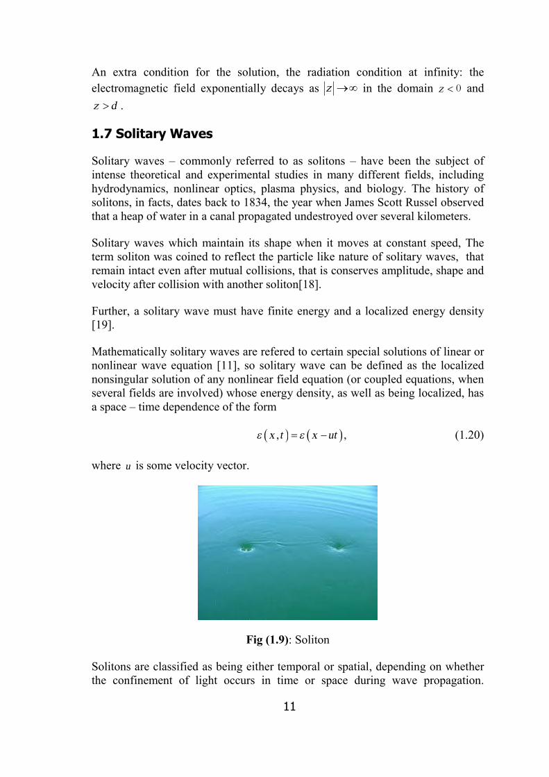
Solitary waves – commonly referred to as solitons – have been the subject of intense theoretical and experimental studies in many different fields, including hydrodynamics, nonlinear optics, plasma physics, and biology. The history of solitons, in facts, dates back to 1834, the year when James Scott Russel observed that a heap of water in a canal propagated undestroyed over several kilometers.

Solitary waves which maintain its shape when it moves at constant speed, The term soliton was coined to reflect the particle like nature of solitary waves, that remain intact even after mutual collisions, that is conserves amplitude, shape and velocity after collision with another soliton[18].

Further, a solitary wave must have finite energy and a localized energy density [19].

Mathematically solitary waves are refered to certain special solutions of linear or nonlinear wave equation [11], so solitary wave can be defined as the localized nonsingular solution of any nonlinear field equation (or coupled equations, when several fields are involved) whose energy density, as well as being localized, has a space – time dependence of the form

( ) ( ), ,x t x utε ε= − (1.20)

where u is some velocity vector.

Fig (1.9): Soliton

Solitons are classified as being either temporal or spatial, depending on whether the confinement of light occurs in time or space during wave propagation.

12

Temporal solitons represent optical pulses that maintain their shape whereas spatial solitons represent self-guided beams that remain confined in the transverse directions orthogonal to the direction of propagation solitons naturally arise in several areas of mathematical physics, such as in nonlinear optics, fluid mechanics, plasma physics, condensed matter, particle physics, astrophysics, and quantum field theory [20].

Solitons, in general, manifast themselves a large velocity of wave particle systems in nature. Particularly in any system that posses both dispersion (in time or space) and nonlinearity.

The inherent importance of solitons in real life comes from the fact that, as soon as the field intensity is high enough for the nonlinearity to play a role, the system is governed by nonlinear modes, rather than linear ones. In most cases, these modes are solitons [16].

A number of integrable models - exactly solvable models in statistical physics- have soliton solutions, with well-known behaviour in propagation and collisions. These includes

(i)Firstly in general any localized static (time independent )solution is a solitary wave with velocity 0=u in equation (1.20) [19].

(ii) The Kortewege de viries (kdv) equation which is a model of waves on shallow water surface which describes the small amplitude dark solitons and it's equation is given by:

2 0.t x xxxυ υυ s v+ + =

(iii) The second partial differential equation representing solitons is the Sine-Gordan Equation (SGE) which given by:

( )sin .tt xxxν ν ν− =

This equation has been used in the study of a wide range of phenomena, including propagation of crystal dislocations of splay waves in memberence, of magnetic flux in Joesephson lines, Blochwall motion in magnetic crystals [19].

(iv) The Nonlinear Schrodinger Equation (NLS) is given by:

2 0.t xxiν ν ν ν− + =

This equation recently has been intensively studied because it describes the propagation of pluses of laser light in optical fiber [21].

13

CHAPTER 2

Preliminaries

In this chapter we introduce the fundamental concepts of Weierstrass elliptic function which are needed throughout this thesis.

2.1 Weierstrass elliptic function

2.1.1 Def init ion of Weierstrass e l l ipt ic funct ion

Let \,w w be complex or real numbers such that the ratio \/w w is not real. Then consider the lattice – the additive subgroup of C – generated by \,w w [22]:

\2 2 : ,mw nw m nΩ = + ∈¢ (2.1)

Weierstrass function ( ) ( )\/ ,z z w w℘ =℘ is an elliptic function of periods \2 , 2w w which is of order two, has a double pole at z = 0 and can be expressed

by the series [2]

( )( ) ( )

\

2 22 \ \,

1 1 1

2 2 2 2m nz

z z mw nw mw nw

℘ = − −

− − + ∑ (2.2)

This sum is over all points of / 0Ω , and this series converges absolutely and uniformly except near its poles, namely the points of Ω . ( )z℘ represent a one – valued function of z, regular except for the points of Ω . Therefore ( )z℘ is analytic through the whole z – plane except at the points of Ω , where its has double pole.

Definition 2.1 [22]

If ( )z℘ is a Weierstrass ℘ – function with fundamental periods 2wand \2w ,

where ( )\Im / 0w w > , define the numbers 1 2 3, ,w w w by:

\ \1 2 3, ,w w w w w w w= = + =

and the number 1 2 3, ,e e e by ( ) 1,2,3.i ip w e i= =

14

2.1.2 Integral representation of ( )z℘

Theorem (2.2) [23]: The function ( )z℘ satisfies the differential equation

( ) ( ) ( )\\ ,z z g z g℘ = ℘ − ℘ −32 34 (2.3)

where the elliptic invariants 2 3,g g are given by,

( ) ( )\ \

2 34 6, ,1 2 1 2

1 160 , 140 .2 2 2 2m n m n

g gz mw nw z mw mw

= =+ + + +

∑ ∑ (2.4)

An alternative form of the differential equation in the last theorem is

( ) ( ) ( ) ( )\ \ z z e z e z e ℘ = ℘ − ℘ − ℘ − 1 2 34 (2.5)

This shows that 1, 2,3ie i = are the roots of the algebraic equation 3

2 34 0t g t g− − =

Now, conversely, given the equation

23

2 34dz t g t gdu

= − −

(2.6)

and consider the equation [24]:

32 34u

dtzt g t g

∞

=− −

∫

(2.7)

Which determines z in terms of u . The path of integration may be chosen to be any curve not passing through a zero of 32

34 gtgt −− .

After differentiation, we have

23

2 34dz u g u gdu

= − −

And it follows that

( )u z A=℘ +

For a constant A.

15

Now if we let u tends to infinity, then z tends to zero, as the integral converges. Therefore, A is a pole of the function ( )z℘ . It follows that ( )u z=℘ . Therefore we can write

( )u

dtut g t g

∞−℘ =

− −∫1

32 34

(2.8)

Definition(2.3) [25]: Throught this thesis, 32 , gg are defined as in theorem (2.2) and are called the invariants of the ℘– function. We also define the discriminant ∆ of ( )z℘ by

( ) ( ) ( )2 2 23 22 3 1 2 1 3 2 327 16 .g g e e e e e e∆ = − = − − − (2.9)

2.1.3 Properties of Weierstrass function

Theorem (2.4)

The function ( )z℘ is an even function of z; it satisfies the equation: [22,23]

( ) ( )z z℘ =℘ −

Proof:

Now the set of points - Ω is the same as those of Ω , so we have that the terms of the absolutely convergent series:

( ) ( )\

2 2, 1 2 1 2

1 1m n z mw nw mw nw

− + + +

∑

Are the terms of the series

( ) ( )\

2 2, 1 2 1 2

1 1m n z mw nw mw nw

− − − +

∑

Rearranges that, and since the series is absolutely convergent, this change in order does affect the value of the sum of the series; and therefore we have

( ) ( )z z℘ =℘ − (2.10)

16

Further, the function ( )z℘ admits the quantity 12w as a period [22]

( ) ( )z w z℘ + −℘12

( ) ( ) ( ) ,m n

z w z z w mw nw z mw nw− − −−= + + + + − − − − −∑2 2 221 1 1 2 1 22 2 2 2 2 2

( )( ) ( ) ,z m w nw z mw nw− −= − − − − − −∑ 2 2

1 2 1 22 1 2 2 2

Where the last summation is extended over all integer and zero values of m and n without exception. But this last sum is zero, since its terms cancel each other in pairs. Thus we have:

( ) ( ).z w z℘ + =℘12 (2.11)

Similarly ( ) ( )z w z℘ + =℘22 and generally ( ) ( )z mw nw z℘ + + =℘1 22 2 where m and n are any integers.

2.1.4 The addition formula for the function ( )z℘

The function ( )z℘ possesses an addition formula which gives the value of

( )z y℘ + in terms of the value of ( )z℘ and ( )y℘ where z and y are any quantities [24].

( ) ( ) ( )( ) ( ) ( ) ( )

\ \z yz y z y

z y ℘ −℘

℘ + = −℘ −℘ ℘ −℘

214

(2.12)

If we put 1y w= , then ( )\ w℘ =1 0 , ( )w e℘ =1 1 and hence we obtain:

( )( )

( ) ( )

\ zz w z e

z e

℘℘ + = −℘ −

℘ −1 12

14 (2.13)

( ) ( )( )

e e e ee

z e− −

= +℘ −

1 2 1 31

1

Similarly,

17

( ) ( )( )( )

e e e ez w e

z e− −

℘ + = +℘ −

2 1 2 31 2

2 (2.14)

And

( ) ( ) ( )( )

.e e e e

z w ez e

− −℘ + = +

℘ −3 1 3 2

3 33

(2.15)

2.1.5 Descriptive properties of Weierstrass function

We shall describe briefly the behaviour of ( )z℘ for real 2g and 3g , distinguishing two cases according to 2

332 27gg −=∆ as it is positive or negative.

(1) First, let 0>∆ , then the primitive periods are such that w is real and \w is purely imaginary. The point lattice of all the periods may be generated by a rectangular, in this case 321 eee >> and 03 <e . As z describes the boundary of the

rectangle \ \

, , , ,w w w w+0 0 , the function ( )z℘ decreases from ∞ to ( )e w=℘1 , to

( )\e w w=℘ +2 to ( )\e w=℘3 to ∞− .

(2) Now, let 0<∆ , this case is very different from the first one, and again there is a pair one periods, however there exists a pair of conjugate complex primitive periods giving a rhombic fundamental parallelogram.

In this case only 2e is real and 31,ee are conjugate complex numbers. As z varies along diagonals of period parallelogram frokm 0 to \

w w+ to w2 (or \w2 ) ( )z℘ decreases from ∞+ to 2e to ∞− [24].

Degenerate cases of Weierstrass function occur when one or both of the periods become infinite, or equivalently, two or all three of 321 ,, eee coincide then the three case are:

(i) Real period infinite:

aeaee 2, 321 −===

∞=ω

(ii) Imaginary period infinite:

\

, ,e a e e a iω= = = − = ∞1 2 32

18

(iii) Both periods infinite:

\

,e e e i iω ω= = = = − = ∞1 2 3 0

In all three cases 0=∆ .

Figure (2.1)

Fundamental period parallelogram of Weierstrass elliptic function

19

CHAPTER 3

Existence of Eigen Waves and Solitary Waves in Lossy Linear and Lossless Nonlinear Layered Waveguide

Introduction:

In this chapter we consider the electromagnetic waves propagation in the system of three – layered structure where the film and semi – infinite substrate layer is homogenous dielectric nonmagnetic linear and the other half semi-infinite cladding is linear homogenous magnetic with permeability µ fillful with metamaterial, this case is of particular interest in linear optics. [26]

Also we consider the case where the film has nonlinear permittivity depending on the field intensity.

3.1 Geometry of the problem

We treat the problem of electromagnetic wave propagation in the satisfied medium, with the permittivity:

( ), ,, ,, ,

zz z d

z d

εε ε

ε

<= < < >

2

1

3

00 (3.1)

where Im 0 , 2,3j jε = = and either ( ) ,iε ε α α= + ≥1 1 1 0 with a real constant or

( )2011 1 Ec+= εε with real constant, and depending on the magnitude of the field

intensity.

The electric field component has the form:

( ) ( )i Bz wtyE e z eϕ −=

r (3.2)

where ey = (0,1,0)T is the unit vector along the y-axis

By section 1.5 E satisfies Eq. (1.15) and Eq. (1.16) and consequently ϕ satisfies

( ) ( ) ( )\ \ z k n zϕ ε ϕ− + − =2 20 0 (3.3)

20

( )( ) ( ) ( )\ \

where the layer is nonmagnetic.If the layer is magnetic metamaterial then

z k n zϕ εµ ϕ− + − =2 20 0

The geometry of the problem is shown in figure (3.1), the layers are infinite a long y– axis and x– axis.

Figure (3.1)

Geometry of the problem

3.2 Solutions to differential equation if ( )α1εε 1

_

1 i+=

We will begin with the linear case where ε2, ε3 are real and ( )1

_

1ε ε 1 αi= + [24], So assume that α> 0 (the central layer is lossy)

case 1: n2< min ε3µ3 , ε2 then n2 - εiµi< 0

So the solution of (3.3) has the form : [26]

21

cos sin , ,

( ) , ,

cos sin , ,

k z n k z n

A k z n A k z n z

z Be Ce z d

D k z n D k z n z

ε ε

ε ε

ϕ

ε µ ε µ

− − −

− + − <= + < <

− + − >

2 20 1 0 1

2 22 0 2 1 0 2

2 22 0 3 3 1 0 3 3

0

00

(3.4)

where A1, A2 or (D1, D2) are uniquely determined by other coefficients.

Case 2 : If min ε2, ε3µ3 ≤ n2 <∧ε = max ε2,ε3µ3,

Then there are two cases:

Firstly, If ε3 µ3,≤ n2 <ε2 and ε3 ≠ ε3µ3 then 022 >−εn and so the general

solution of Eq. (3.3) in the substrate layer is :

2 2K n εμ K n ε 2 2(z) A e Be

z zϕ

− − −= +o o (3.5)

And the solution of Eq. (3.3) in the other layers is as in (3.4).

Now since z→-∞, the exponential 2k n ε

2z

e− −

o blows up and is physically unacceptable (due to radiation condition |E|→0 as z→∞). Thus in this region z < 0 the solution is physically acceptable if B = 0 . So the solution is

( )k z n

z Aeε

ϕ−

= o2

2. (3.6)

Secondly,

If ε3µ3 ≤ n2 < ε2 then 0332 >− µεn and so the general solution is this region

(z>0) is :

-k01(z) D ek z n z ne Dε µ ε µϕ − −= +

2 20 3 3 3 3

2. (3.7)

Similarly as in equation (3.6) this solution is physically acceptable only if D1= 0 then the wave function decays exponentially as z goes to ∞ , So the solution is:

( ) k z nz D e ε µϕ − −=2

0 3 32

. (3.8)

Case 3: if ε2 = ε3 3µ = n2 substituting in Eq. (3.4) we will show that the solution

in the regions (z > 0) , (z < 0) is constant,

22

Applying the boundary condition to get solution in the region 0 < z < d

12

12

012

0

21

0

0

00

εnC)(B

εnKCεnKB

)(φ`)(φ`

−−=

−−−=

=

So either n2 = ε1 = ε2= ε3µ3 and the solution ϕ (z) = const ∈ ℝ or B=C ≠ 0. Then2 3` (0) ` (0)ϕ ϕ= gives

12

012

01

201

200 εε εε −−− −−−= ndkndk enCKenBK

and hence

112

02 =−εndke

Then n2=ε1 and again the solution ϕ (z)= const ∈ R.

Case 4: If ε2 ≠ ε3µ3 and n2 = max ε2, ε3µ3

(i) If n2 = ε2 > ε3µ3

Then the solution of Eq. (3.3) in the substrate layer is constant and the solution of the cladding layer is similarly to Eq. (3.4) that is:

( ) K z n K z n

K z n

A zz Be Ce z d

De z

ε ε

ε µ

ϕ − − − −

− −

<= − < < >

2 20 1 0 1

20 1 3

00

0 (3.9)

φ(z) satisfies the boundary condition which yield this system of equations:

CBA +=

01212 =−−− εεεε CB

3320120120 µεεεεεε −−−−− =+ dkdkdk DeCeBe

33201201203321212

µεεεεεε µεεεεεε −−−−− −−=−−− dkdkdk eDeCeB

Solving this system of equations we obtain

23

)eeεεeeμεε(εε 33201203120120 μεεdkεεdk12

μεεdkεεdk31212

−−−−−−−− −−−−

+ 0)eeεεeeμεε(εε 33201203320120 μεεdkεεdk12

μεεdkεεdk33212 =−+−− −−−−−−

Multiplying by 0 2 3 30 2 1 0 2 1 k d ε ε μk d ε ε k d ε εe e e ,we get−− − −

__ __

2 1 2 12 ε ε 2 ε ε2 1 2 3 3 2 1 2 1 2 1 2 3 3 2 1 2 1ε ε ε εμ ε ε ε ε ε ε ε εμ ε ε ε ε 0,d de e− −− − − − − + − − + − − =

where = kod

Then

)εεεε(εε)εεεε(εε

1233212

1233212εε2 12

__

−−−−

−+−−=−−

µµde

Leading to the dispersion relation [27]:

12332

12332εε2

εεεεεεεε

12

__

−−−

−+−=−−

µµde (3.10)

(ii) If n2 = ε3µ3> ε2. Therefore the solution is

( )

K z n

K z n K z nAe z

z Be Ce z dD z

ε

ε εϕ

− −

− − − −

<= + < <>

20 2

2 20 1 0 1

00

0 (3.11)

Similarly as the previous case, applying the boundary condition on φ (z) leads to the dispersion relation in this case:

233133

233333εε2

εεεεεεεε

132

__

−−−

−+−=−−

µµµµµde (3.12)

For Eq. (3.10) – and similarly Eq. (3.12), Eq. (3.10) can be written in other way as:

24

ln i kd

ε ε ε ε µε ε ε ε µ π

ε ε ε ε

− + − − − − − = +

− −

2 1 2 3 3

2 1 2 3 3

2 1 2 12 since zkiz ee =+ π2 (3.13)

It is easy to see that ε ε ε ε µ

ε ε ε ε µ

− + −>

− − −2 1 2 3 3

2 1 2 3 3

1 and since the left hand side of

Eq.(3.13) is negative – since d is the thickness of the layer must be positive – then this implies that Eq. (3.13) has solution only if

012 <− εε that is

01 <− εn and 1ε<n

And this is the condition for Eq. (3.10) to have solution.

Similarly for Eq.(3.12), it has solution only if 3 3 1 0ε µ ε− < and hence,

3 3 1n ε µ ε= < .

Case 5: If n2> max ε2, ε3µ3 and α = 0 (then central layer is lossless) then the solution of Eq. (2.1) is:

( )

K z n

K z n K z n

K z n

Ae zz Be Ce z d

De z d

ε

ε ε

ε µ

ϕ

−

− −

− −

<= + < < >

20 2

2 20 1 0 1

20 1 3

00 (3.15)

Similarly as before we get the dispersion relation:

__2

1

2 2 2 2ε ε 1 2 1 3 3

2 2 2 21 2 1 3 3

( n -ε n -ε )( n -ε n -ε )

( n -ε n -ε ) ( n -ε n -ε )de

µ

µ− − + +

=− −

2 (3.16)

For a lossy layer (α > 0):-

Assume that 2

1ε nw = − . Then we have

tan tan( ) .d n

d n

eid n dwe

ε

εε

− −

− −

−− = =

+

21

21

22

1 2

11

(3.17)

25

Substitute Eq.(3.16) in Eq.(3.17) : -

( ) ( ) ( ) ( )( ) ( ) ( ) ( )

( )( )

_tan(d )

n n n n n n n nw

n n n n n n n n

n n n

n n n

ε ε ε ε µ ε ε ε ε µ

ε ε ε ε µ ε ε ε ε µ

ε ε ε µ

ε ε ε µ

− + − − + − − − − − − − −=

− + − − + − + − − − − − −

− − + −=

− + − −

2 2 2 2 2 2 2 21 2 1 3 3 1 2 1 3 3

2 2 2 2 2 2 2 21 2 1 3 3 1 2 1 3 3

2 2 21 2 3 3

22 2 2

1 2 3 3

2

2

( )( ) ( )

( )( ) ( )

iw n n

w n n

iw w w

w w w

ε ε ε ε µ ε ε

ε ε ε ε µ ε ε

ε ε ω ε µ

ε ε ε ε µ

− − + + − − +=

− + − − + − − +

− − − + − −=

− − − − −

2 22 1 1 3 3 1 1

2 2 22 1 1 3 3 1 12 2

1 2 1 3 3

2 2 21 2 1 3 3

So for the Lossy layer ( )0>α we get the set of two equation [27]:

( ) ( )( ) ( )

taniw w w

F w dww w w

ε ε ε ε µ

ε ε ε ε µ

− − − + − −= − =

− − − − −

2 21 2 1 3 3

32 2 2

1 2 1 3 3

0 (3.18a)

and

( ) ( )( )( )

taniw w w

F w dww w w

ε ε ε ε µ

ε ε ε ε µ

+ − − + − −= + =

− − − − −

2 21 2 1 3 3

32 2 2

1 2 1 3 3

0 , (3.18b)

where 2

1ε nw inξ= − = + is a complex variable.

Now we show that there exists a unique complex root of Eq. (3.18). So let us limit ourselves to the consideration of Eq. (3.18a)

If 2

1ε nw inξ= − = + is a complex – valued function in ( , ,ξ η α ), so we write the nonlinear system equivalent to Eq. (3.18a)

26

( ), ,F ξ η α =13 0 where ReF F −=13 3

( ), ,F ξ η α =23 0 where ImF F −=23 3 (3.19)

We assume 0Im,0 ≥≥ nη and 3,2,0Re 2 =>− jn jε .

Set ( ) ( )23133 ,,, FFFw T == ηξ and consider ( )αww = as an implicit function of the

parameter α defined by Eq. (3.18a) and the system (3.19), since ( )_

iε ε α= +11 1 so it may be reduced to caushy problem:

( )αα

,wddw

Φ= (3.20)

If ∗ξ is a real root of Eq. (3.16) then Eq. (3.18a) has *ξ root if α = 0 that is:

( ) ( )* ,T

ow w ξ ∗= =0 0 since 0=η .

Now we can write,

( ) ( )Tw 21,, ΦΦ=Φ α

( ) ( )( )ηα

αα

,,, 31

1 DwFDJw −−=Φ

( ) ( )( )αξ

αα

,,, 31

2 DwFDJw −−=Φ

where ( )( )ηξ

α,

,3

DwFDJ = is the Jacobi determinant,and this determinant is non-

degenerate (meaning that ( ) 0, ≠αwJ unless ( ) 0, =αwJ for all w , so ( ),oJ w ≠0 0 ).

Now by using the implicit function theorem we show that there exists solution for Eq. (3.18).

Theorem(3.1) (implicit function theorem) [28]

Let ∪ be open in 2R and let Rf →∪: be a C 1 - function.

Let ( )ba , be a point of ∪ , and let ( ) cbaf =, . Assume that ( ) 0,2 ≠bafD then there exists an implicit function ( )xy ϕ= which is C 1 in some interval containing c and such that ( ) ba =ϕ .

27

Now In system (3.19) we have:

• ( ), ,oF w =3 0 0 where *( , )Tow ζ= 0 and

• Also since the Jacobi determinant ( )( )ηξ

α,

,3

DwFDJ = is non-degenerate, and the

components of the right hand of Eq. (3.20) is continuously differentiable then by implicit function theorem there exist a unique continuously differentiable solution of ( )αw of the caushy problem (3.20) in a vicinity of 0=α , and consequently, the existence of unique (complex) root of system (3.19) and Eq. (3.18a) for sufficiently small [ ], oα α∈ 0 .

3.3 Solution of the differential equation in the nonlinear film

Now consider the case of a three layer waveguide with a lossless nonlinear central layer with permittivity

( )\c Eε ε= +2

1 01 (3.21)

depending on the field intensity E.

Assume that ε2 ≤n and 32 εε ≠ then the solution of the substrate and cladding is given by Eqs. (3.4), (3.6), (3.8), (3.9), (3.11), (3.15) due to the relation between the parameters n2, ε1, ε2, ε3µ3

Now for the central layer 0 < z < d, substitute Eq. (3.21) into Eq. (3.3) to obtain,

_ __\\ ( ) ( ) ( ) ( )z k n z k z k c zϕ ϕ ε ϕ ε ϕ= − +2 2 2 2 3

0 0 0 0 (3.22)

Integrate Eq. (3.22) :

( )__

\ ( - ) ( ) ( )ock n z k z R kεεΦ = Φ + Φ +

2 2 2 2 2 4 20 0 0 02

(3.23)

where 200 kR is an integration constant.

In this case the general solution of Eq. (3.23) can be expressed by the Weierstrass function [29]:

28

__2

10 0 2 3

n ε( ) ( ik z,g , g ) ,3o

zC

γ − − Φ = ℘ + +

2 2

(3.24)

where g2, g3 are the invariants of the Weierstrass function and γ0 is an arbitrary constant. The invariants are determined [29] by the coefficients of Eq.(3.23).

So for ε2 >n , -if ( )A and A D and D1 2 1 2 are given- then a unique solution for equation is given by:

__2

10 0 2 3

o

-2 n ε( ) ( ik ,g , g )C 3

K z n

K z n

A e z

z z z d

D e z

ε

ε µ

ϕ γ

−

− −

<

−= ℘ + + < <

>

20 2

20 3 3

0

0

0

So this solution includes solitary–wave–like solutions. Since the Weierstrass elliptic function is doubly periodic- as we have seen in chapter 2- so it repeat itself in each fundamental period parallelogram without change in properties. Ttherefore the Weierstrass elliptic function represents a solitary wave solution which will deeply studied in chapter 4.

To get the dispersion relation, suppose, that the electric field at z=0 is E0 and at z =d is Ed

For the region (z < 0) then

( ) ( )\ k nϕ ε ϕ= −2 2 2 2

0 1 (3.25)

Or we can write

\ 22 0

2(n ε )EE k at z= − =2 20 0 0

(3.26)

Similarly, for the region (z > d) at z=d we have

\ 23 3 d(n ε )EdE k µ= −2 2 2

0 (3.27)

29

Now, using the boundary condition then \ , iE E1 is continuous. Then Eq. (3.25) and Eq. (3.26) yields

__

2(n ε ) ( )ocE E R n Eε ε− + + = −2 4 2 20 0 0 2 02

(3.28)

Similarly Eq. (3.27) and Eq. (3.25) yield

____ ε2 2 4 2 21(n ε ) ( )1 0 3 32

CoE E R n Ed d dε µ− + + = − (3.29)

Hence we obtain:

c2 4oR E ( - ) E0 0 2 02

εε ε= − 11 (3.30)

_2 40

0 d dcR E ( ) E2

εε ε µ −= − 11 3 3 (3.31)

By using Eq.(3.30) and Eq.(3.31) we get:

__ __

( ) ( )d dc cE E E Eε ε

ε ε µ ε ε− − + − − =4 2 2 41 0 1 01 3 3 0 1 2 0 0

2 2 (3.32)

Now Eq. (3.32) is quadratic in Ed , so that it has the following solution:

2__ __ __ __ __2 2 2 4

1 3 3 1 3 3 0 1 0 1 2 0 1 02

0

( ) ( ) 2 ( )d

c E c EE

cε ε µ ε ε µ ε ε ε ε− ± − − − +

= (3.33)

Hence, after setting

__

( , )d onE ik d g g

Coε

γ− −

= ℘ + −2

10 2 3

23

(3.34)

We obtain:

__ _ _ _ _

,( , ) ( ) ( ) ( )ni d g g c E c Eεγ ε ε µ ε ε µ ε ε ε ε

−− ℘ + − = − ± − − − +

222 2 2 41 1 1 20 2 3 1 3 3 3 3 0 1 0 0 1 02 2

3 (3.35)

30

Here the dispersion relation is expressed entirely in Eq. (3.35) in terms of the initial parameters (ε1, ε2, ε3µ3, co).

For instance 2dE must be real so the expression in Eq. (3.34) under the root sign

must be positive and also the right – hand side Eq. (3.35) must be positive to

keep 2dE > 0 [30].

To determine the number γ0, set A = E0. Then since ϕ (z) is continuous at z = 0 we obtain:

__

( , , ) nE g gc

εγ

− − = ℘ + 2

10 0 2 3

0

23

Thus,

__

( , , ) c E ng g εγ

− −℘ = −

2 210 0

0 2 3 2 3 (3.36)

Finally as in the linear case, by reduction to Cauchy problem as in Eq. (3.20) we can prove the existence of roots for Eq. (3.35) for sufficiently small d (thin nonlinear film) and 0c (weak nonlinearity) and 3µ (permeability) of the metamaterial medium which is negative.

3.4 Conclusion

In chapter 3 we find out the solution of wave equation , and in each case we formulate the solution in each layer, and derive the dispersion relation and we discussed the linear lossy and nonlinear lossless central layer.

We notice that the metamaterial cladding with negative permittivity and negative permeability has affect all equation, since the permeability μ < 0, specially in the dispersion relation and the existence of solitary wave solution.

31

CHAPTER 4

TE Polarized Guided by a Lossless Nonlinear Three – layer Structure

TE polarized electromagnetic waves guided by a three layer structure consisting of a film surrounded by semi – infinite media are investigated in this chapter.

All three media are assumed to be lossless, isotropic and exhibiting a local kerr – like dielectric nonlinearity. In this chapter we consider the permittivity depending on the field intensity E

r on the three layers and we express the solution of the field

equation in terms of Weierstrass elliptic function. We derive general necessary and sufficient conditions for the existence of physical (real, nonnegative, bounded and consistent with the dispersion relation) field intensities.

4.1 Introduction

The TE polarized waves are supported by nonlinear a three – layer structure with permittivity [29]

>+ε<<+ε

>+ε=ε

dzEadz0Ea

0zEa

2

cc

2

ff

2

ss

(4.1)

Assuming that , aν νε are constants, and again the guided stationary TE waves are represented by electric field:

( )0y w,z,nEeE =r

(4.2)

The real amplitude function ( )0w,z,nEE = must be a solution to Eq. (1.15)

aE k q E E k Cz

νν ν νµ

∂ − − = ∂

22 2 2 20 02

(4.3)

with the constant of integration vC that can be determined by the boundary conditions and

2 2q nν ν νε µ= − , , ,s f cν = , (4.4)

where s refers to substrate layer, f refers to film layer and c to cladding layer.

32

Also forµ = 1 ,v s f and= forµ < 0 v c= . Since the cladding is metamaterial, then Eq. (4.3) has a solitary wave like solutions: [29]

( ) ( ), , ; , vv v v v

v v

qE n z w w ik z g ga µ±

= ℘ ± +

22

0 0 2 32

3 , (4.5)

where

( )2 20

31 1 2 3,0,2 3

, ,4

v v v v

v

v va E n w q

dIw v s fI g I g

µ

∞

−

= =− −

∫ (4.6)

( ), ,c c c c

c

v va E n d w q

dIw ik dI g I g

µ ±

∞

−

± =− −

∫2

0

0 31 1 2 32 3

4 (4.7)

v v v v vg a C qµ = +

42

223

(4.8)

v v v v vg a C qµ = +

43

2 43 9

(4.9)

Substituting in Eq. (2.9), then the discriminant ν∆ of the Weierstrass’s function ℘ can be written as:

( )v v v v v v v va C a C qµ µ∆ = +2 2 2 42

( ) ( ) ( )2v3v1

2v3v2

2v2v1 IIIIII −−−= , (4.10)

where vvv III 321 ,, represent the roots in definition (2.1) and they can be written as:

v v v vv v

q a qI Cµ= + +

2 4

1 6 2 4,

v v v vv v

q a qI Cµ= − +

2 4

3 6 2 4 (4.11)

3qI

2v

v2 = .

33

4.2 Real, Nonnegative and bounded field intensities

In this sections we give the condition of solvability (CS) of the dispersion relation (DR) in the nonlinear case. And condition for which ( )vE z±

2 must be real and nonnegative and bounded (CRNB) for all z according to equation (4.1).

As a result, all these conditions and the allowed normalized thickness dk0 can be expressed in terms of Weierstrass's function ℘, it is half periods, and the associated quantities fffff IIIww 321 ,,,,, ±∆

The electric field must satisfy,

0E → as z → ∞ (4.12)

Then Eq. (4.3) with Eq. (4.12) imply that

cs CC == 0 . (4.13)

Substituting this condition in equation (4.10) then we get:

0,s c∆ = ∆ = (4.14)

In this case we have,

4 42 3

4 8,3 27v v v vg q g q= = .

Using the substitute 2

31

vqc = then

3v3

2v2 c8g,c12g == .

Using the relation ( ) ( )

11 2

1 22 3 2;12 ,8 3 sin 3z c c c c c z

℘ = − +

[28] with the above

notation in Eq. (4.5), we have:

( )( )

, ,sin

v v vv

cw ik z g g cc w ik z

℘ ± = − + ±

0 2 3 20

33

34

( )sinv

v

v v

qqq w ik z

= − + ±

22

2 20

13

. (4.15)

Substituting Eq. (4.15) in Eq. (4.5) we obtain

( ), ,v v v v vv v

E w ik z g g qa µ±

= ℘ ± + 2 2

0 2 32 1

3

( )

2

2 20

2 , ,sin

v

v v v v

q v s ca q w ik zµ

= = ±

(4.17)

subject to the condition:

0q2v ≥ ; (4.16)

that is 2 0n ν νε µ− ≥ and so 2 ,n ν νε µ≥ where νµ is the permeability of the metamaterial.

If 0q2v < , then 2

vE ± does not satisfy condition (4.12)l

Now, evaluate Eq. (4.17) using the relation [6]:

yxiyxz sinhcoscoshsinsin +=

to get

( )[ ]=± zikwq vv 022sin

( ) ( )( ) ( )

2 2 2 2 2 2 20 0

2 2 2 20 0

sin Re cosh Im cos Re cosh

2 sin Re cos Re cosh Im sinh Im

v v v v v v v v

v v v v v v v v

q w q w k z q w q w k z

i q w q w q w k z q w k z

± − ± +

± ±

(4.18)

Now, if 2,0 ±< vvv Ea µ is real and nonnegative only if,

0Resin 2 =vv wq

also if 2,0 ±> vvv Ea µ is real and nonnegative then

0Recos 2 =vv wq

35

which yields the necessary and sufficient conditions for 2 , ,E s cν ν± = to be real and nonnegative [3].

2

2

0,

Re 12 0,

v v

v

n

v v

v

l if aq

w

if aq

πµ

π πµ

<= + >

(4.19)

with Zl ∈ and subject to 2 0qv ≥ ,

but if the layer is metamaterial then νµ < 0 and hence Eq. (4.19) becomes

2

2

0,

Re 12 0,

v

v

n

v

v

l if aq

w

if aq

π

π π

>= + <

If 2 0,vq = then Eq. (4.3) becomes:

40

20

2

2Eak

ZE vvµ−=

∂∂ .

so the only possible case is that 0<vva µ (aν < k 0 if the layer in nonmagnetic , and aν > 0 if the layer is metamaterial) with 0=l since the left side is positive.

According to Eq. (4.18) and the properties of xx sinh,cosh then ( )zEv2± is bounded

only if 0cos =x that is 0>vva µ (aν > 0 if the layer in nonmagnetic , and aν < 0 if the layer is metamaterial). In this case

( )( ) ( )

.sin Re cosh Im

vv

v v v v v v

qE za q w q w k zµ

± = ±

22

2 2 2 20

2

Now, for 0<vva µ we have the field intensity as

36

( )( ) ( )cos Re sinh Im

vv

v v v v v v

qE za q w q w k zµ

± = − ±

22

2 2 2 20

2

which is only bounded for ( )zEs2− (for which 0<z so 0Im >vw and 0Im 0 >− zkwv )

and for ( )zEc2+ ( 0>z so )0Im 0 >+ zkwv

Before deriving condition for real, nonnegative and bounded field intensity CRNB, it is suitable to make use of the boundary conditions at the interfaces at 0z = , and

.z d= Since both 2 , ,E s cν ν± = and its derivatives with respect to z are continuous [3] then :

sins

s s s

qEa q w

=2

20 2 2

2 and

sin ss s

s

qq wa E

=2

220

2 then

arcsin ss s

s

qq wa E

=2

220

2

arcsin ss

ss

qwa Eq

=2

220

21 (4.20)

And similarly at dz = we have:

( )sinc

d

c c c c

qEa q w ik dµ

= ±

22

2 20

2 evaluating as previous we get:

arcsin cc

c c dc

qw ik da Eq µ

± =2

0 22

21 (4.21)

Now, if ( )2 2 ,0, 00 0E E n ws= > , using the continuity of derivative at 0z = then

| |0 0

dE dEs fdz dzz z

== =

(4.22a)

and by Eq. (4.3) we can write:

37

s ss

dE ak q E Edz

= −

22 2 2 20 0 02

, (4.22b)

f f

f vdE ak q E E k Cdz

= − +

22 2 2 2 20 0 0 02

(4.22c)

Now by Eq. (4.22a) we have

s fs f f

a aq E E q E E C − − − =

2 2 2 2 2 20 0 0 02 2

Now, substitute ,s s f fq n q nε ε= − = −2 2 2 2 we obtain [29],

( )f f s f sC E a a Eε ε = − − −

2 20 0

12

(4.23)

Now we prove that Eq. (4.20), and Eq. (4.21) are consistent with Eq. (4.19).

In Eq. (4.15) the relation [6] is used:

( ) ( ) ( )

−+−+−+= 2

12 1ln1arcsin1arcsin ααβπ ikz kk , (4.24)

where

( )[ ] ( )[ ]21

2221

22 1211

21 yxyx +−+++=α ,

( )[ ] ( )[ ]21

2221

22 1211

21 yxyx +−−++=β ,

Considering that

2 20 , 00q Es ≥ >

then we have, Firstly, If sa < 0 then s

s

qa E

<2

20

2 0 and hence s

s

qa E

2

20

2 is pure

imaginary, and using relation (4.24)

( ) 0By1 21

2 =+=α

so we have

38

( ) ( )12

2 220

2arcsin 1 ln 1Ls

s

q L i y ya E

π

= + − + +

Now by Eq.(4.20) we have:

Re ( ) Re arcsin ss

ss s

qw La Eq q

π= =2

22 20

21 1

Since sa < 0 then sa E <20 0 and then:

ss

a Eq >2

2 0

2 (4.25)

Now, if sa > 0 then s

s

qa E

>2

20

2 0 that is s

s

qa E

2

20

2 is real again using relation (4.24),

1Bx ==α

So

( ) ( ) ( )arcsin lnL Ls

s

q L i x xa E

ππ

= + − + − + −

12 2

20

2 1 1 12

so ( )Re arcsin Ls

s

q La E

ππ= + −2

0

2 12

that is

2

1Re2s

s

w Lq

ππ = +

which is consistent with Eq. (4.16), now 2 1 0α − ≥ so

ss

a Eq >2

2 0

2 (4.26a)

Similarly for 0Re( )cw ik d± and

( )c c cc

a E dq

µ ±>2

2

2 (4.26b)

in the metamaterial layer.

Using properties of Weierstrass function ℘, the following necessary and sufficient condition for ( )zE2

f ± to be real [24] are obtained:

39

0Re Re , 0f f fik z L ifω ω ω= ± = ∆ > (4.27)

and

0 2Re , 0,f fik z L ifω ω± = ∆ < (4.28)

must hold, where ω , 2ω are the associated real half-periods of P. subject to conditions (4.25) – (4.28), ( )fcsvv ,,=ω can be written down, and they contain elliptic integrals which can be simplified by using the roots fff III 321 ,, defined in Eqs. (4.10) – (4.11)

Ordering the roots fff III 321 ,, according to:

maxmin III m <<

we introduce ffof IEaI 2202

1+=

Then by Eq. (4.6) we have:

∫∞

−−=

fIff

fgIgI

dIw0

3234

(since 1=fµ )

so we can get a sufficient condition for real ( )zE f2

± from Eq. (4.27) and Eq.(4.28) as follows:[29]

(i) If 0>fa and 0>∆ f then

maxIII ofm ≤< (4.29)

(ii) If 0<fa and 0>∆ f then

minIIof < , since 0<ofI (4.30)

or

maxIII ofm <≤ (4.31)

(iii) If 0<fa and 0<∆ f then

40

fof II 2< (4.32)

For the case 0>fa and 0>∆ f is impossible due to Eq. (4.27).

By the previous Eqs. (4.29) – (4.32), we can find the bounded, and nonnegative field intensities (solitary-wave-like solution). And since the Weierstrass elliptic function is periodic, so we will limit our consideration to fundamental period parallelogram FPP as shown in figure (2.1).

If wwf =Re , the solitary-wave-like solution is:

( ) ( ), ,f f f f ff

E z ik k g g qa

ω± = ℘ ± +

2 20 2 3

2 13

( )( )Im , , .f f f ff

i k z g g qa

ω ω = ℘ + ± + 2

0 2 32 1

3

Using the addition theorem given in section (2.1.4) for ( )( )Im fi k zω ω℘ + ± 0

where ( ) maxIω℘ = , then we obtain[3]:

( ) ( )( )( )( )

max max minmax

max, ,m

f ff m f f f

I I I IE z I q

a i I w k z g g I±

− −= + +

℘ ± −

2 2

0 2 3

2 13

( )( )( )( )

max max minmax

max

., ,

mf

f m f f f

I I I II I

a i I w k z g g I

− −= − +

℘ ± − 2

0 2 3

2 (4.33)

Now, since ( )( ) min, , ,m f f fi I w k z g g I−∞ ≤℘ ± ≤0 2 3 Eq. (4.33) represent a

bounded solitary-wave-like solution ( )zE f2

± for all z.

Now Eq. (4.33) can be written,

( )( )( ) ( ) ( )( )

( )( )max max max max min

max

, ,, ,

m f f f f mf

f m f f f

i I k z g g I I I I I I IE z

a i I k z g g Iω

ω±

℘ ± − − + − − = ℘ ± −

0 2 3 22

0 2 3

2

and since

( )( )( ) m ax m in m axIm , ,f f fi k z g g I I Iω℘ ± − < −0 2 3

41

Then ( )zE f2

± is nonnegative if only if

0>fa and fff III 321 ,> (4.34)

or 0<fa and 2 1 .f fI I> (4.35)

(i) If ( )00Re >∆= ffω then the field intensity ( )zE f2

± becomes:

( ) ( )( )Im , ,f f f f ff

E z i k z g g Ia

ω± = ℘ ± − 2

0 2 3 22 (4.36)

It is clear that ( )zE f2

± is nonnegative only if 0,fa < since

( )( )Im , ,f f f f fi k z g g I Iω−∞ ≤℘ ± ≤ <0 2 3 3 2

From figure (2.1), we have the following necessary and sufficient condition for

( )zE f2

± to be bounded

izkf

\

02Im0 ω

ω <±< (4.37)

due to the location of poles of ℘(z) since 0, i

\2ω are poles of ℘(z) – where \ω is

the imaginary half – period of ℘.

(ii) Now, if ( )Re f fω ω= ∆ <2 0 . And using again the addition theorem of ℘(z) then the solitary-wave-like ( )zE f

2± can be written as:

( ) ( )( )( )( )Im ; ,

f f f f ff f

f f f f f

I I I I qE z Ia i k d g g Iω ω±

− −= + +

± −

22 1 2 32

20 2 3 2

23

( )( )( )( )Im ; ,

f f f f

f f f f f

I I I Ia i k d g g Iω ω

− −=

± −

2 1 2 3

0 2 3 2

2

But since ff II 31 , are complex conjugate for 0<∆ f then the field intensity becomes [3]:

( ) ( )( )Im ; ,f f

ff f f f f

I IE z

a i k d g g Iω±

−=

℘ ± −

22 12

0 2 3 2

2 (4.38)

42

Since if 0<∆ f then ( )\ , ,f f fg g Iω℘ =2 2 3 2 , by figure (2.1) we have ( )zE f2

± is bounded and nonnegative if 0<fa and

\ \Im k zω ω± <2 0 2

(4.39)

Where \2w is the imaginary half – period of ℘(z).

Finally we can summarize the physical content of the forgoing analysis as follows:

(i) If 0>∆ f and max0min III f ≤< ( )Re ,fω ω= 0>fa then fII 1max = must hold and 0<fa then fII 2max = must hold for nonnegative ( )zE f

2± . Also ( )zE f

2±

is bounded everywhere. (ii) If 0>∆ f and ( )0Remin0 =< ff II ω ( )ωω =fRe then 0<fa is a sufficient

condition for nonnegative ( )zE f2

± and i

zkf

\

02Im0 ω

ω <±< for bounded

( )zE f2

± .

(iii) 0<∆ f and ff II 20 < then 0<fa and \20Im ωω <± zkf are a sufficient

conditions for nonnegative and bounded ( )zE f2

± .

For ( ) csvzEv ,,2 =± as we stated before ( )zEs2± and ( )zEc

2± are bounded if 0>vva µ ,

and if 0<vva µ then only ( )zEs2− and ( )zEc

2+ are bounded.

So if the parameters 20 0, , , , ,v va n E k dνε µ do not fulfill the previous conditions,

then there is no guided waves exist. And if irrespective of dk0 , the parameters

ff a,∆ are such that 0,0 <∆> ffa then according to Eq. (4.28) there is no guided wave exists.

In the next section we specify the normalized thickness that obey CRNB. in order to get sufficient conditions for existence of guided waves.

4.3 Solutions of the dispersion relation

If the boundary conditions are satisfied, then beside Eqs. (4.20), (4.21) and (4.23), the following equation must be satisfied [29]:

( ) ( ), , ,f f f f ff f

E d w ik z g g Ia a

λ± ± = ℘ ± − = 2

0 2 3 22 2 (4.40)

where

43

,2 1

f c

c c

f

Daa

ε ελ

µ±

−= ±

−

(4.41)

2

,2 1 2 1

f c f f

c c c c

f f

a cDa aa a

ε εµ µ

− = +

− +

(4.42)

Now condition (4.25) becomes:

2 2c cc f

f

aq Eaµ

±> due to boundary conditions and substituting 2±fE from Eq. (4.40)

to get,

2 c cc

f

aqaµ

λ±>

Subject to the previous section the imaginary part of ( )0 2 3, ,f f fik z g gω℘ ±

vanishes, so the right hand side of

( ), ,f f f fik z g g Iω λ±℘ ± = +0 2 3 2 (4.43)

Then fI2+±λ must be real if and only if ±λ is real iff 0≥D . Also 2±fE is

nonnegative then 02≥±λ

fa if and only if

±= λsgnsgn fa (4.44)

Eq. (4.43) is a compact representation of DR, and if we prescribed one of the parameters 2

0 0, , , ,v va E k dνε µ then the rest of parameters can be determined, but since these parameters are embedded in ff gg 32 ,,±λ then we can't use Eq. (4.41) to determine one of these quantities, but we can only use it to verify the existence of guided waves.

Since ±λω ,,, 32 fff gg and fI2 are independent of dk0 in Eq. (4.41) we will solve it with respect to dk0 and find the associated (CS).

Now let

44

21

033 2 3

( ).4fq f

f f

dI ik dI g I gλ

ω ω±

∞ −± +

= =℘ ±− −

∫

(4.45)

By theorem (2.3) , Eq. (2.8) and Eq.(4.40) we have,

23

3 2 34fq

f f

dII g I gλ

ω±

∞

± +± =

− −∫ (4.46)

\

f ik d M Nω ω ω= ± + +0 2 2

where \2 , 2ω ω are the complex periods of ℘, M, N, are integers.

\fik d M Nω ω ω ω±= ± − + +0 2 2 for 2

+fE (4.47a)

and

\fik d M Nω ω ω ω±− = ± − + +0 2 2 for 2

−fE (4.47b)

Eq. (4.47) hold for real and positive dk0 so we can write Eq. (4.47) as a system [3],

( )\Re f M Nω ω ω ω±± − + + =2 2 0 (4.48a)

( )\Im f M N k dω ω ω ω±± − + + = 02 2 for 2+fE (4.48b)

and

( )\Im f M N k dω ω ω ω±− ± − + + = 02 2 for 2−fE (4.48c)

To find the condition of solvability for equation (4.43) (with dk0 real and positive) it is useful to consider the CR of the previous section, since the CS are analogous to the CR.

(i) 0>∆ f , \Re ,f w i IRω ω= ∈ , without loss of generality assume that

( )Im fi k dω ω+ + 0 FPP∈ . Since function ( )( )Im , ,f f fi k d g gω ω℘ + + 0 2 3

decreases monotonically from Imax to Im if \

Im ,f k di

ωω

± ∈

0 0 and increases

monotonically from Im to Imax if \ \

Im ,f k di i

ω ωω

± ∈

0

2 . So each value

45

[ ]max,mI I℘∈ is taken twice if

∈±

idkf

\

02,0Im ω

ω ; thus, the condition of solvability

is

( )( ) maxIm , ,m f f fI i k d g g Iω ω≤℘ + + ≤0 2 3 (4.49)

Then by Eq. (4.40), and Eq. (4.49) can be written as

max2 III fm ≤+≤ ±λ (4.50)

which is identical to Eq. (4.31) with 202

1 Ea f replaced by ±λ , now since ωω =fRe

and 1ω is purely imaginary then Eq.(4.48) can be written as

( )Re 2 0,Mω ω ω±± − + = (4.50a)

( )\Im .fk d Nω ω ω+= ± − + =0 2 0 (4.50b)

for +fE , and

( )\Im fk d Nω ω ω+− = ± − + =0 2 0 (4.50c)

for ( )zE f\

−

Now,

\ .f ik d M Nω ω ω ω± = ± + +0 2 2 (4.51)

Then

( ) ( )Re Re 2 .f Mω ω ω± = +

But Eqs. (4.50) is equivalent to,

( ) ( ) ωωω ==± fReRe (4.52)

Hence, for Eq. (4.50a)

( ) 02Re =+− ωωω M so 0=M

or

46

( ) ( )( )Re 2 0 Re 2 1 0.M Mω ω ω ω− − + = = − − = So 1=M

and the positive normalized thickness given by Eq. (4.50b) and Eq. (4.50c) can be written as[3]:

( )

( )( )

\

\

Im

Im , , ... sin

Im , , ,...

f f

f

f

if a E

k d N if N this is ce k d is positive

N if N

ω ω λ

ω ω ω

ω ω ω

+ +

+

+

− >= − + = − −

− − + =

20

0 0

12

2 1 2 3

2 2 3 4

(4.53)

for 2+fE , and

( )

( )( )

\

\

Im

Im , ,

Im , , , ....

f f

f

f

if a E

k d N if N

N if N

ω ω λ

ω ω ω

ω ω ω

− −

−

−

− − <= − + + =

+ + + = −

20

0

12

2 1 2 3

2 1 0 1 2

(4.54)

associated with 2−fE .

This is true without further restriction since ( )zE f2

± is bounded for ωω =fRe by Eq. (4.33).

(ii) 0>∆ f and 0Re =fω then ( )zE f2

± is represented by Eq. (4.38).

Now, ω ∈¡ , \iω ∈¡ then if ( ) FPPdki f ∈± 0Imω . ( )z℘ increases monotonically

- if x < y then ( ) ( )x y℘ <℘ - from ∞− to 3e if ( )\

Im ,fi k di

ωω

± ∈

0 0 and ( )z℘

decrease monotonically - if x > y then ( ) ( )x y℘ >℘ - from 3e to ∞− as

( )\ \

Im ,fi k di i

ω ωω

± ∈

0

2 then ( )( ) ] ]0 3Im ,fi k d eω℘ ± ∈ −∞ and since 03 <e

then we get the necessary condition

min2 II f ≤+±λ (4.55)

Using Eq. (4.51) again to get,

±== ωω Re0Re f (4.56)

47

Then Eq. (4.48a) reads

( ) ( )0)2Re2Re ==+−± ± ωωωω MMf if and only if 0=M

For the normalized thickness dk0 , by Eq. (4.37) we have:

\

Im Imf fk diω

ω ω− < < −02

for 2+fE and

\

Im Imf fk d foriω

ω ω− < <02

2

−fE

These inequalities together with Eqs. (4.48 b)(4.48 c) we have,

( )

( )\

Im

Im

f f

f

if a Ek d

ω ω λ

ω ω ω

+ +

+

− >= − − +

20

0

12

2 (4.57)

Associated with 2+fE and

0 ,fk d ω ω−= − + (4.58)

20

12 fwhere a Eλ− <

(iii) 0<∆ and \2 2 2Re ,f R and i iω ω ω ω= ∈ ∈ R , then by figure (2.1) the

primitive periods of ℘ are \,ω ω ω+2 22 and we can see that if

( ) FPPdki f ∈±+ 02 Imωω then ( )( )Im fi k dω ω℘ + ±2 0 increases monotonically

from ∞− to 2e as dkf 0Im ±ω ranges from \

toω− 2 02

, and decreases

monotonically from 2e to ∞− as dkf 0Im ±ω ranges from \

to ω− 202

which yield

that

( )( )Im ,f fi k d Iω ω℘ + ± ≤2 0 2

2 2 .f fI Iλ± + ≤

48

And so we have:

0.λ± ≤ (4.59)

Again by Eq. (4.51)

2Re Re .fω ω ω± = = (4.60)

And hence Eq. (4.48a) read,

( )( )\Re f M Nω ω ω ω ω±± − + + + =2 2 22 0 (4.61)

( )2Re 2 0.f M Nω ω ω±± − + + = (4.62)

Then either

( )( ) 02Re 2 =++−+ ± ωωω NMf

and by Eq. (4.60) then ( )2 2 22 0M Nω ω ω− + + = yield 02 =+ NM

or ( )( ) 02Re 2 =++−− ± ωωω NMf and similarly then 22 =+ NM

Also by Eqs. (4.46.b,c) the normalized thickness is given by for this case:

( )\Im ,f fn k d for Eω ω ω± +± − + = 22 0 (4.63)

and

( )\Im .f fn k d for Eω ω ω− −− ± − + = 22 0 (4.64)

Evaluate Eq. (4.39) then we have:

\ \Im Imf f fk d for Eω ω ω ω +− − < < − 22 0 2 (4.65)

\ \Im Imf f fk d for Eω ω ω ω −− < < + 22 0 2 (4.66)

Now, Eq. (4.63) together with Eq. (4.65) can be written as: [3]

( )( )

−−

>−=+

++

f

ff Eaifdkωω

λωω

Im21Im 2

00 (4.67)

49

Associated with 2+fE . And

( ) 20 0

1Im2f fk d if a Eω ω λ− −= − + > (4.68)

For bounded 2−fE .

In order to find the physical solution fcsvEv ,,2 =± for the given normalized thickness given by Eqs. (4.53), (4.54), (4.57), (4.67) and (4.68) we have to find the right field intensities csvEv ,2 =± which match ( )zE f

2± at the boundaries, so

we look for the combination of signs of the field intensities,

( )2

0 2 30

2 , ,|sf f f

sz

dE dik w g gdz a dz

±

=

℘= ±

And we can easily see that

sz

s adz

dE sgnsgn |0

2

±==

± (4.69)

And similarly for cv = ,

2

sgn|cc c

z d

dE adz

µ±

=

= ± (4.70)

that is 2

sgn|cc

z d

dE adz

±

=

= ∓

For 2±fE , ( )fff

fdz

f ggdkpikadz

dE320

\0

,0

2

,,2| ±=

± ±= ω

\

,|

f z d

k p ia

ε=

±= 0

0

2 (4.71)

where ( )

dzggdkpd

p fff 320\ ,,+=

ω

And \

\

pp

=ε

50

For ( )dkiu ff 0ImRe ±= ωω where 2,0,Re ωωω =f and the sign of dz

dE f2

± depends

on the sign of fa together with ε , In figure (4.1) which represents the fundamental period parallelogram for 0>∆ f in the left side and 0<∆ f on the

right one together with ε , then one can notice that the sign of dz

dE f2

± depends on

the magnitude of fωIm and 0Im Im( )k dω± = ± that depends on the mode equation (4.50 b,c)

Fig (4.1)

FPP for Positive and negative discriminants ∆f , \

\

pp

=ε denotes the normalized

derivative of Weierstrass function ℘(u)

4.4 Guided waves in a structure with linear substrate and film and nonlinear cladding.

As an application we take the case 0.fa = Then the discriminant f∆ vanishes;

( )2 2 42 0.f f f f f fa c a c q∆ = + =

This case has been excluded in the analysis in the previous sections.

In previous analysis the basic assumption was that 0≠fa , but if 0=fa then some of the results of section (4.3) become meaningless.

51

For example, if we choose Eq. (4.27) then ω becomes infinite and according to Eq. (4.11) then ff II 21 = and since 02 <fI then 01 <fI which leads to 02 <fq , and also fω defined in equation (4.40) becomes undefined.

So it seems rather involved to evaluate the results of section (4.2, 4.3) in the limit 0→fa . Thus, it is appropriate to go back to Eq.(4.3) and solve it subject to

conditions (4.13), (4.16), (4.25) and (4.26). Hence,

( ) 00 ,fq k z

sE z E e= 0≤z

( ) 0 0 0cosh sinh , 0sf f f

f

qE z E q k z q k z z dq

= + < <

(4.72)

( )( )

,sin

cc

c c c c

qE z za q ik zµ ω

= ≥±

2

20

2 1 0

where cω is given by Eq. (4.21), also according to Eq. (4.17) with 0c ca µ > we have ( )zEc± is bounded.

Using the continuity of E and dzdE at z = d, we find

( )( )

2

0 0 0 20

2 1cosh sinhsin

s cf f f

f c c c c

q qE d E q k z q k dq a q w ik dµ±

= + =

± (4.73)

and

( ) ( ) ( )( )

2202

0 0 0 2 20

cos2sinh coshsin

c ccf f f c

c c c c

q w ik dqE d q q k d q k d i qa q w ik dµ

±= + = ±

± (4.74)

From Eq. (4.73) we get:

( )( )

2 2

2 20

12 sin

c cf c

c c

a E d qq w ik d

µ=

±

Then ( )( )

2 2 2 2

2 20

12 sin

c cc f c c

c c

aq E d q qq w ik d

µ− = −

±

52

( )( )

2 2 2

2 20

112 sin

c cc f c

c c

aq E d qq w ik d

µ − = − ±

2 202

2 20

cos.

sinc c

c

c c

q w ik dq

q w ik d

±= −

±

This implies that:

( )2

02 2 2

20

cos2 sin

c cc cc c f c

c c

q w ik daq q E d i qq w ik d

µ ±= − =

±%

Now substitute cq~ and Eq. (4.73) in Eq. (4.74) to have:

( )0 0 0 0 0 0sinh cosh cosh sinhsf f s f f f c

f

qE q q k d q q k d E q k d q k d qq

+ = ± +

% (4.75)

Now divide Eq.(4.75) by dkq f 0cosh to get:

0 0tanh tanh ,sf f s c c f

f

qq q k d q q q q k dq

+ = ± +

% %

0tanh .sf f c c s

f

qq k d q q q qq

= ± −

% %∓

So,

0tanh .s cf

s cf

f

q qq k d q qqq

= −

%∓%

∓ (4.76)

Thus, we get the dispersion relation[3]:

( )0 2tanh 0,f s c

ff s c

q q qq k d

q q q+ =

%∓%∓

(4.77)

where the upper and the lower signs refers to ( ) ( )zEandzE cc −+2 respectively.

53

The dispersion relation resembles the linear one provided that

( )2 2

2c c

c c faq q E dµ

= −% , according to Eq. (4.22) cq~ is real and cc qq =~ if only if

0=ca .

In this case Eq. (4.77) is reduced to the linear dispersion relation.

Now square both sides of Eq. (4.74) to get:

( )2 24

2 020 0 0 4 2

0

cos2sinh coshsin

c ccf f s f

c c c c

q w ik dqE q q k d q q k da q w ik dµ

±+ =

± (4.78)

Using the trigonometric identitiy 2 2cos 1 sinz z= − , we obtain

( )( ) ( ) ( )

2

4 4 2

cos 1 1 ,sin sin sin

zz z z

= −

Substituting this and Eq. (4.73) in Eq. (4.78) we have:

( )( )

4240 0 04

220 0 0 22

cosh sinh22sinh cosh

2

c c sf f

fcf f s f

c c c

a qE q k d q k dqqE q q k d q q k d

a q

µ

µ

+ + = −

240 0 0cosh sinh

2c c s

f ff

a qE q k d q k dq

µ +

then,

( )4

22 40 0 0 0 0 0 0sinh cosh cosh sinh (cosh

2c c s

f f s f f f ff

a qE q q k d q q k d E q k d q k d q k dq

µ + = − + − +

)sinh 0dkq

qq

ff

s

So,

54

420 0 0cosh sinh

2c c s

f ff

a qE q k d q k dq

µ + =

( )2

0022

00 sinhcoshcoshsinh

+−+ dkq

qqdkqqdkqqdkqq f

f

sfcffff

Finally we have[3]:

( )2

2 20 0 0 0

20 4

0 0

sinh cosh cosh sinh

2cosh sinh

sf f s f c f f

fc c

sf f

f

qq q k d q q k d q q k d q k dqa E

qq k d q k dq

µ

+ + + =

+

(4.79)

We can use this version to find the parameters 20 0, , , , ,c c va n E k dµ ε which is

compatible with the dispersion relation.

4.5 Conclusion

In this chapter we have derive the condition for nonnegative, bounded, real field intensity E where the permittivity in three layers is nonlinear and described the kerr-law, and we have also derive the normalized thickness (dispersion relation) and finally, as an application we study the case af = 0.

55

CHAPTER 5

TE-Guided Waves in a three Layer Structure with Kerr–type Nonlinearity

5.1 Introduction

In the previous chapters we considered propagation in a three – layer structure for which the film has the permittivity

2

fff Ea+ε=ε of the central layer (film) with fε being constant. In this chapter we consider the more general case. We assume that ( )zff ε=ε is a real – valued continuous function of the transverse z,

and the other semi – infinite nonlinear media with permittivties 2

Eavvv

r+= εε

where ,v vaε are constant and vε does not depend on z – transverse (in the substrate s and cladding c layers).

5.2 Formulation

Here, we consider the more general case when the permittivity is

( ) ( )

≥+ε<<+ε

≤+ε=ε

dz,Eadz0,Eaz

0z,Eaz

2

cc

2

ff

2

ss

(5.1)

where ( ) ( )i k nx wtE z eϕ −= 0 also satisfies Eqs. (1.12), (1.13) that is:

( )\\ v vv

az k q µϕ ϕ ϕ − − =

2 2 20 0

2 (5.2)

with ( )zϕ must satisfy the conditions in section (1.6).

The solution of Eq. (5.2) in the underlying layer ( )cv = is [4]

( ) ( ),

cosh sinh

ss

ss s s s

q Eaq k q z q E k q z

ϕ =− −

0

2 20 0 02

(5.3)

56

( ) ( ),

cosh sinh

c dc

c cc c c c

q Eaq k q z d q E k q z d

ϕµ

= − − − −

2 20 0 02

where .v vq n υε µ= −2 2 Then by Eq. (4.25) and Eq. (4.26b) we have

,s c cs c

a aq E q Eµ≥ ≥2 2 2 2

0 02 2 and 0E 0 > and dE are real constants. It follows that

,s cϕ ϕ satisfy the boundary conditions at 0=z and dz =

( )0 0fE ϕ= (5.4)

and

( ) ( )

( ) ( )

sinh cosh

cosh sinh

ss s s s s s

s

ss s s s

a Eq E k q k q z k q q k q zddz aq k q z q E k q z

ϕ

− − −

=

− −

22 2 0

0 0 0 0 0

22 2

0 0 0

2

2

| |s s fs

z z

d a dE k q Edz dzϕ ϕ

= == − =2 2

0 0 00 02 (5.5)

Similarly for cϕ we have

( ) ( )c d fd E dϕ ϕ= = (5.6)

| |c c c fd c

z z d

d a dE k q Edz dzϕ µ ϕ

= == − − =2 2

0 00 2

Note that Eq. (5.4) – Eq. (5.6) are valid for any sign of ( ),a s cν ν = . Now we will consider the solution in the central layer dz0 << . Eq. (5.2) is equivalent to the Volterra equation [4]

( ) ( ) ( ) ( ) ( )( ) ( )sinhzf

f f f ff

k q z tz z k t a t t dt

qϕ ϕ δ ϕ ϕ

−= − +∫ 0 2

0 00

(5.7)

with ( ) ( )sinh fk q z tz t

q−

− =k 0 is the kernel, and with fϕ satisfies Eqs. (5.5) –

(5.6). The function ( )0 zϕ is defined by

57

( ) ( ) ( )cosh sinhsf s f

az E k q z q E k q zϕ

= + −

2 20 0 0 0 02

(5.8)

when 0a f = . We can find the solution of by interaction or successive approximations, and we begin with the approximation [5]:

( ) ( )0f z zϕ ϕ≈ (5.9)

This approximation is equivalent to saying that 0k or the integral is small. We then put this crude choice into integral equation under the integral sign to obtain a second approximation

( ) ( ) ( ) ( ) ( )01 0 0 0

0

sinhzf

f

k q z tz z k t t dt

qϕ ϕ δ ϕ

−= − ∫ (5.10)

and then the process is repeated and we obtain,

( ) ( ) ( ) ( ) ( )2 0 0 0 10

sinhz

fz z k k q z t t t dtϕ ϕ δ ϕ= − − =∫

( ) ( ) ( ) ( )00 0 0

0

sinhzf

f

k q z tz k t t dt

qϕ δ ϕ

−= +∫

( ) ( ) ( ) ( )0 1 0 120 0 1

0 0

sinh sinhz z

f f

f f

k q z t k q t tk t t dt dt

q qδ ϕ

− −∫ ∫ (5.11)

This series can be written formally as:

( ) ( )0

,f jj

z zϕ ϕ∞

=

= ∑ (5.12)

where

( ) ( ) ( ) ( )00 1

0

sinhzf

j jf

k q z tz k t t dt

qϕ δ ϕ −

−= − ∫

(5.13)

for any bounded function ( )tδ .

In the nonlinear case ( )0a f ≠ solution ( )f zϕ has the form of the limit function of the uniformly convergent functional sequence ( ) 1,2,..j z jϕ =

58

where

( ) ( )j fz zϕ ϕ→

and

( ) ( ) ( ) ( ) ( ) ( )sinhzf

j f j jf

k q z tz z t a t t dt

qϕ ϕ δ ϕ ϕ− −

− = − + ∫ 0 2

0 1 10

(5.14)

With the sufficient condition for a uniform convergence of Eq. (5.14) in the form

( ) ( ) ( )sinhmax

zf

fz df

k q z tdt t a z

qδ ϕ

≤ ≤

− + < ∫ 0

000

427

(5.15)

which it will be proved next section.

The solution calculated by formulas (5.7) – (5.10) at dz = must satisfy the condition (5.4) – (5.6).

Now ( ) ( ) ( ) ( )( )0 20 0

0

sinhdf

d f f f ff

k q d tE d d k t a dt

qϕ ϕ δ ϕ ϕ

−= = − +∫ (5.16)

and

( ) ( )( )02 2 200 0 0 0

0

cosh| |

2

dfc cf

d c f f f fz d z d f

k q d ta dd k E q E k k q t a dtdz dz q

µ ϕϕδ ϕ ϕ

= =

−= − − = − +∫

( ) ( )( )2 2 2 200 0 0 0

0

| cosh2

dc c

d c f f f fz d

a dk E q E k k q d t t a dtdz

µ ϕδ ϕ ϕ

=− − − == − − +∫ (5.17)

Substituting for dE from Eq. (5.16) we get,

( ) ( ) ( )( )0 2 2 200 0 0 0

0

sinh|

2

df c c

f f f cz d f

k q d td ak d k t a dt q Edz qϕ µ

ϕ δ ϕ ϕ=

−− − − − + −

∫

( ) ( )( )2 20 0

0

coshd

f f f fk k q d t t a q dtδ ϕ= − − +∫ (5.18)

So

59

( ) ( ) 2 200 0 0, |

2c c

cz d

d aF n a k d q Edz

ϕ µϕ

=

+= − − +

r

( ) ( ) ( )( )02 2 20 0 0

0

sinhcosh

2

dfc c

f c f f ff

k q d tak k q d t q E t a dtq

µδ ϕ ϕ

−− + − +

∫ (5.19)

which yields the dispersion relation:

( ), 0,F n a =r (5.20)

where n is the spectral parameter and ( )0, , , , , ,s c f c va a E dε ε ε µ=r is the vector of

nonspectral parameter.

5.3 Convergence of iteration

5.3.1 Linear case

First, the case 0aaa fcs === is considered. we will prove that the series

( ) ( ) 10 0

z

jj

K z t t dtδ ϕ∞

−=

− −∑ ∫ uniformly converges on [0,d] to continuous function fφ

(z).

Denoted ( ) ( ) ( ),k z t t z tδ= −K

Lemma: 5.1 [31]

( ) ,!

jj

jzz kj

ϕ ϕ≤ 0 (5.21)

where ( ),

max ,z t d

k k z t≤ ≤

=0

Proof:

We prove this by induction, first for j=1 we use Eq. (5.13) we have

( ) ( ) ( ),z

z k z t t dtϕ ϕ= −∫1 00

.z

k dt k zϕ ϕ≤ =∫0 00

(5.22)

60

Now, assume that it’s valid for j, then for j+1 we obtain the inequality,

( ) ( ),z

j jz k z t dtϕ ϕ+ ≤ ∫10

( ),z

jk z t dtϕ≤ ∫0

(5.23)

The lemma is true for j, so substitute 0 !

jj

jzkj

ϕ ϕ≤ in Eq. (5.23) to get,

( )!

jzj

jtz k dtj

ϕ ϕ++ ≤ ∫

11 0

0

( )1

10 .

1 !

jj zk

jϕ

++≤

+ (5.24)

Remark (5.2):

The solution ( )f zϕ of Eq. (5.2) represented by the series (5.9) is converges uniformly on [0,d]

Proof: ( ) ( ) ( )0 0

f j jj j

z z zϕ ϕ ϕ∞ ∞

= =

= ≤∑ ∑

According to (5.21) then

( )!

jj

fj

zz kj

ϕ ϕ∞

=

≤ ∑ 00

!

j jz k

j

zk ej

ϕ ϕ∞

=

= =∑0 00

(5.25)

which yield the estimate for ( )f zϕ in the space [ ]( 0, )c d

0 .d kf eϕ ϕ≤ (5.26)

Now we will prove that ( ) ( )0

p zf z e δϕ ϕ=

61

for j=1 we have, ( ) ( ) ( )z

k z t t t dtϕ δ ϕ= −∫1 00

( ) sinh coshzf f

f f

q t q zt dtq q

ϕ δ ϕ δ ϕ−

≤ =∫1 0 0 20

1 (5.27)

and for j=2,

( ) ( ) ( ) ( )z

t k z t t t dtϕ δ ϕ= −∫2 10

( ) cosh sinhzf f

f f

q t q tt dtq q

ϕ δ ϕ−

≤ ∫2

2 0 20

1 (5.28)

Using the subtitle 1tqcoshu f −=

dttqsinhqdu ff=

dtq

tqsinhqdu

f

f2f

=

So the integral in inequality (5.28) becomes:

( )4f

2f

1zqcosh

0

1zqcosh

04f

2

4f q2

1zqcoshq2

uduquf

f| −==∫

−− (5.29)

Substitute Eq. (5.29) in (5.28) to get,

( ) ( )2 22 0 ,t p zϕ δ ϕ≤ (5.30)

where

( ) cosh .f

f

q zp zq

−= 2

1

assume it is true for j, then

( ) ( )0j j

j t p zϕ δ ϕ≤

we prove it is true for j+1,

62

( ) ( ) ( ) ( )z

j jt k z t t t dtϕ δ ϕ+ = −∫10

( ) cosh sinhjz

j f fj

f f

q t q tt dtq q

ϕ δ ϕ++

−≤

∫

11 0 2

0

1

using the previous way to evaluate the integral we get

( ) ( )1 11 0

j jj t p zϕ δ ϕ+ +

+ ≤

which gives

( )( ) ( )0

00 0 !

jjp z

f j jj j

p zz e

jδϕ δ

ϕ ϕ ϕ ϕ∞ ∞

= =

= = =∑ ∑ (5.31)

which complete the uniform convergence of the series (5.9) since δ is a bounded function.

5.3.2 Nonlinear case

Considering the case 0, 0 0.s c fa a and a≠ ≠ ≠ Assuming that ( )zδ is continuous in (5.7), we solve the Volterra Eq. (5.7) by using the sequence of the functions (5.14).

Donating

( ) ( ) ( )max maxz

fz d z dc z a z k z t dtδ ϕ

≤ ≤ ≤ ≤

= + − ∫2

0 0 00 0 (5.32)

and assuming that 1c0 < .

Lemma 5.3[31]: The estimate

0jj a φ≤φ (5.33)

holds for j=1,2,… with 1aac1a 03

1j0j =+= − (5.34)

Proof: We prove it by induction. So firstly setting j=1, we obtain

63

( ) ( ) ( )( )z

fz z t t a dtϕ ϕ δ ϕ ϕ= − − +∫k 21 0 0 0

0

( ) ( )max maxz

fz d z dt a z t dtϕ δ ϕ

≤ ≤ ≤ ≤

≤ + + − ∫ k2

0 00 00

1 (5.35)

( )0 01 cϕ= +

and since a0 = 1

( )( )z c aϕ ϕ≤ + 31 0 0 01 (5.36)

Now, assume it is true for all 1j ≥ , we prove that it is valid for 1j + ,

( ) ( ) ( )z

j f j jz z t t a dtϕ ϕ δ ϕ ϕ+ ≤ + − + ∫ k

21 0

0 (5.37)

Substituting ( )j jz aϕ ϕ≤ 0 then:

( ) ( ) ( )z

j f j jz z t t a a a dtϕ ϕ δ ϕ+

≤ + − + ∫ k

2 21 0 0

01

( )30 0 0 11 j jc a aϕ ϕ +≤ + = (5.38)

Which completes the proof of the Lemma.

Lemma 5.3 [31]: For every j=0,1,2,…. The estimate

31 0 0j j jc aϕ ϕ ϕ+ − ≤ (5.39)

holds, where ja are determined from (5.34).

Proof:

Firstly, for 0j = ,

( ) ( )z

fz t t a dtϕ ϕ δ ϕ ϕ − = − + ∫k 21 0 0 0

0

64

( ) ( )max maxz

fz d z dt a z t dtϕ δ ϕ

≤ ≤ ≤ ≤ ≤ + − ∫ k

20 00 0

0

30 0 0 0 0c c aϕ ϕ= = (5.40)

Now, from Eq.(5.10) we have,

( ) ( ) ( ) ( )z z

j j f j j f jz t t a dt z t t a dtϕ ϕ δ ϕ ϕ δ ϕ+ + + − = − + − − + ∫ ∫k k2 21 2 1

0 0

( ) ( ) ( )

z

j j f j f jz t t t a a dtδ ϕ δ ϕ ϕ ϕ+ + = − − + − ∫k 3 31 1

0

( ) ( )z

j j f j j j jz t t a dtϕ ϕ δ ϕ ϕ ϕ ϕ+ + + ≤ − − + + ∫ k 2 2

1 1 10

(5.41)

Now, assume that inequality (5.39) holds for any j where 0j ≥ . We will prove it is true for 1j + we find the upper bound of the right hand side of (5.41)

Substituting of 1,j jϕ ϕ+ from (5.33) the right hand side of (5.41) becomes

( ) ( ) ( )z

j j f j j j jz t t a a a a a dtϕ ϕ δ ϕ+ + + − − + + + ∫k 22 2

1 1 1 00

(5.42)

Using (5.32) and (5.39) then (5.42) becomes

( )2jj1j

21j0

3j00 aaaa.c.ac ++φ≤ ++ (5.43)

To complete the proof, it sufficient to show

( ) ( )33j0

2jj1j

21j

3j0 ac1aaaaac +≤++ ++ (5.44)

In order to prove this inequality we choose a 0c that satisfies

( )0 31 .21

c forαα

α≤ ≤

+ (5.45)

Now by (5.28) we have j1j aa >+ . Using this in the left hand side of (5.44) we get:

65

( )3 2 2 3 20 1 1 0 1.3 .j j j j j j jc a a a a a c a a+ + ++ + ≤ (5.46)

Condition (5.45) yields

( )0 34 1 1 .

27 21jc for and aα

α αα

≤ = ≤ ≤ ++

Then for any j

123

274.2ac2

33j0 =

≤

and thus the right hand side for (5.46) becomes

21j

3j0

21j

3j0

21j

3j0 a.aca.ac2aac3 +++ +=

21j

3j0

21j a.aca.1 ++ +=

( ) ( )33j0

31j

3j0

21j ac1aac1a +==+= ++

This completes the proof.

Lemma 5.4 [31]: If 274c0 ≤ for certain

21

≤α , then the sequence in (5.10)

converges in [ ]( )0,C d to a continuous function ( )zq f that satisfies equation (5.7).

Proof:

We prove that ( ) , 1,2,...j z jϕ = is a caushy sequence in [ ]( )d,0c . Indeed

.....j p j j p j p j jϕ ϕ ϕ ϕ ϕ ϕ+ + + − +− ≤ − + + −1 1 hold. (5.47)

We estimate 1jforjpj ≥φ−φ + . In what follows, we will assume that

( ) ( ) ( ) 2

00max . 1.ft z d

z a z k z tδ ϕ≤ ≤ ≤

+ − ≤ (5.48)

The nonlinearity parameter fa and the film thickness d must be taken sufficiently small.

66

Using induction, we prove the inequality

( ) ( ) ( )( )!

j

j j j

zz z a

jϕ ϕ ϕ

+

+ − ≤+

13

1 0 1 (5.49)

For j = 0, it follows from (5.10) and (5.48) that

( ) ( ) ( ) ( )z

fz z z t t a dtϕ ϕ δ ϕ ϕ − = − + ∫k 21 0 0 0

0

( ) ( )max .z

ft z dt a k z t dtϕ δ ϕ

≤ ≤ ≤ ≤ + − ∫

20 00

0 (5.50)

Then using (5.48) we get

( ) ( ) .z

z z dtϕ ϕ ϕ− ≤ ∫1 0 001

0 .zϕ=

which proves (5.49) for 0j = because 1a 0 =

Now, assume that (5.49) holds for every 0j ≥ we prove that it will be valid for the subsequent value j+1,

( ) ( ) ( ) ( )z

j j j j f j j j jz t t a dtϕ ϕ ϕ ϕ δ ϕ ϕ ϕ ϕ+ + + + + + − = − − + + + ∫k 2 2

2 1 2 1 1 10

( ) ( ) ( )z

j j f j j j jk z t t a a a a a dtϕ ϕ δ ϕ+ + + ≤ − − + + + ∫

2 2 21 0 1 1

0

Using (5.48) and (5.49) we get,

( ) ( )!

jz

j j j j j j jza a a a a dtj

ϕ ϕ ϕ+

+ + + +− ≤ + ++∫

13 2 2

2 1 0 1 10 1

( ) ( ) !

j

j j j j jza a a a aj

ϕ+

+ += + ++

23 2 2

0 1 1 2 (5.51)

Using (5.44) then,

67

( )( ) ( )! !

j jj j

j j

c a az zc j c j

ϕ ϕ ϕ ϕ+ +

++ +

+− ≤ =

+ +

33 32 20 1

2 1 0 00 0

12 2

(5.52)

Now, using (5.49) then (5.47) can be written as:

( ) ( )....

! !

j j pj

j p j p j p

a d dac j j p

ϕ ϕ ϕ+ +

+ + − + −

− = + + + +

3 13

1 0 10

11

( )( ) ( ) ( )

....!

jd d dc j j j j

αϕ

+ +≤ + + + + + + +

31 2

00

1 11 2 2 3

This is true since ,....2,1jfor1a j =α+≤

10

20

011

2

jd as jdc jj

ϕα +

≤ → → ∞+ −

+

The Lemma is proved.

5.4 Existence

To verify the existence of the solution we consider the permittivity with 0=== fcs aaa , so we can write

( )

>≤≤

<=

00

020

zdz

zzk

c

f

s

εεε

ε (5.53)

with real constant cs εε , and ( )zfε is a real – valued continuous function of the transverse coordinate z on [0,d].

( )\ \c c nϕ ε µ ϕ− = − 2 if 0>z and 0<z

and

( )( )\ \fn zϕ ε ϕ− + − =2 0 if dz ≤≤0

So Eq.(5.2) can be written in the form:

( )\\ q zϕ ϕ λϕ− + = (5.54)

68

where,

( ) ( ) 00

c c f z z dq z

otherwiseε µ ε − ≤ ≤

=

(5.55)

and 2c c nλ ε µ= − .

Theorem 5.5 [31]:

Assume the following conditions are satisfied:

(i) For a given continuous function ( ) [ ]( )dzzf ,0∈ε and positive constants cε and sε there exists at least one eigenvalue of equation (5.54).

(ii) The function ( ) ( ) 0ff zz εεδ −= and a positive constant 0

fε are such that the

number 0c defined by (5.32) satisfies the condition 274

0 <c .

(iii) Inequality (5.48) holds.

Then there is a sufficiently small 0>∗fa such that for all faz = ( )0, fa∗∈

then there exists a solution to the Helmholtz equation (5.2).

According to (5.3), (5.10) the corresponding root ( )ξnn = of the dispersion equation (5.20) exists and simple.

Proof:

Assume that (i), (ii), (iii) are satisfied, then as known in [32] equation (5.47) with compactly supported potential q -supp ( ) ( ) 0, ≠∈= zqZzq the set of points where q is not zero-.

Then equation (5.54) has nontrivial solution with at most finitely many eigenvalues 1.... ββ −<<− n , Clearly if λ is an eigenvalue then λ is negative and of multiplicity one[33]. (this includes that the number of eigenvalue may be zero).

Now for a given ( )zfε continuous function, then there exist at least one eigenvalue ∗= λλ which is equivalent to existence of simple root λε −== ∗

cnn where ( ) 00, =∗nF and hence

0| ≠∂∂

∗=nnnF (5.56)

69

holds.

Also, if ( )zq is not – compactly supported potential ( )sc εε ≠ , then according to [33] there exist finite set of eigenvalues of finite multiplicity.

Now for 0== cs aa and 0≠fa by (i) for a given continuous function ( )zfε there exists at least one eigenvalue and hence there exist at least one simple root ∗= nn of the dispersion relation (5.20), and one negative eigenvalue

2αελ nc −=∗ of equation (5.54) of the multiplicity one. Consider equation (5.20) for fixed

00, , , , , ,s c f v ca E dε ε ε µ . Then in the vicinity of n , ( ), ,F n

nξ ξ

∂=

∂0 is continuous and

we also have

( )

≠∂∂

∗=

∗

0|

0,

nnnF

nF

Applying implicit function theorem yields that there exist a continuous function ( )ξn in small vicinity of 0, == ∗ ξnn .

Now, we will determine the range of variation of the film layer normalized thickness d , (in the form of a nonempty domain) D in the ( )ξ,d plane.

Assume that ( )csvavv ,,, =ε and 0fε are fixed, and consider the continuous

function ( )zfε and ( )∗∈ a,0ξ then the corresponding root ( )ξnn = ( )21,nn∈ where

in are positive. So we can do the estimates,

( ) sinh .f

f

q uk uq

=

So

( ) ( ) ( )dMQ

dQtzk

f

f

dzt 00

sinhmax =≤−

≤≤≤ ,

022 ff nQ ε−= (5.57)

where ( ) 00 →dM as 0→d

Similarly, substitute this in 0ϕ to get

70

( )0 1M dϕ ≤ where ( ) ( ) ( )

−+= 2

02

001 2cosh EaQdMdQEdM s

sf

(5.58)

where ss nQ ε−= 22

2 .

Now, we can write the inequalities,

( ) ( )[ ]2742

1001 <+ dMdM ξδ (5.59)

which yield condition (5.26) with 21

=α , and

( ) ( )[ ] 12100 ≤+ dMdM ξδ (5.60)

which yield condition (5.41), and ( )zδδ =0

Clearly, for every ξ , there exists such that the inequalities (5.59), (5.60) satisfied when [ ]0,0 dd ∈ . So the solution to these inequalities specifies a subdomain

1D D⊂ where (5.11), (5.32), (5.48) hold.

5.5 Conclusion

In this chapter we deal with TE polarized waves supported by lossless kerr-like nonlinear three layer structure modeled by permittivity given in (5.1), and we

give the condition for the existence of a solution of helmohltz equation, this solution is a limit function ( )zϕ0 of uniformly convergent series of functions and then we prove the existence and uniqueness of function n=n(af) a solution of the dispersion relation (5.20).

We can consider in future studying the planner waveguide structure formed for three layer in which the film is metamaterial and derive the wave equation in this case and the dispersion relation.

71

Reference

[1] W. Hayt and J. Buck, Engineering Electromagnetics, McGraw- Hill, New York, (2012).

[2] N. Engheta, and R. Ziolkowski, Metamaterial Physics and Engineering Explorations, John wiley & Sons inc., New York, (2006).

[3] H.W Schurman S Serov, and Yu. Shestopalv, TE-Polarized Waves Guided by A lossless Nonlinear Three-layer Structure, Physical Review E, Vol 58, No 1, PP 1040-1051 (1998).

[4] H. Schurmann, S Serov, and Yu. Shestopalv, Propagation of TE Waves Through A layer Having Permittivity Depending on the Transverse Coordinate and Lying Between Two Half–infinite Nonlinear Media, Doklay mathematics, Vol 60, No2, pp 286-288, (1999).

[5] T. Chow, Mathematical Methods for Physicists: A concise Introduction, Cambridge University Press, UK, (2000).

[6] M. Abramowitz and I Stegun, Hand Book of Mathematical Functions with Formulas, Graphs and Mathematical Tables, National Bureau of Standards Applied Mathematics Series 55, USA, Ninth printing, (1970).

[7] R. Hunsperger, Integrated Optics, Springer, USA, (2009).

[8] F. White, Electromagnetic Waves, John & Wiley inc., New York, fourth edition, (1950).

[9] S. Mendhe, and Y. Kasta, Metamaterial Properties and Application: International Journal of Information Technology and Knowledge Management, Vol 4, No 1, PP 85-89, (2011).

[10] K. Alici, E. Ozbay, A planner metamaterial: Polarization independent fishnet structure, Phonotics and Nonostructues : Fundamental and Application, Vol 9, PP 15-21, (2011).

[11] S. Gunduz, M. Cakir, C. Cakir, and L. Sevgi, Metamaterial and FTDT based Numerical Modeling Studies, zeamet sok. No 21,Libra.masra.cn/publication/14109260/ metamaterials.and-ftdt-based-numerical-modeling-studies.

[12] E. Kazantseva, A. Miamistov, and S. Ozhenko, Solitary Electromagnetic Waves Propagating in the A symmetric Oppositely Directed Coupler, pp 1-9,(2009). arxiv.org/abs/ 0904.4035.

[13] M. Golovkina, Electromagnetic wave propagation in multilayed structures with negative index material. www.intechopen.com

72

[14] C. Caloz, C. Chang, and t. Itoh, Fall-wave Verification of the Fundamental Properties of the Left-handed Materials in Waveguide Cefigurations, Journal of Applied Physics, Vol 90, N 11, PP 5483-5486, (2011).

[15] Y. Frenkel, Propagation of Ultra–short Electromagnetic Pulses in A maxwell Doffing Medium, New York, (2008).

[16] N. AkhmeDiev, Spatial Solitons in Kerr and Kerr-Like Media, Optical and Quantum Electronics, vol 30, pp 535-569, (1998)

[17] A.D Boardman, P. Egan, R. Mitchell-Thomas, Y. Rapoport, and N. King, Weakly and Strongly Nonlinear Waves in Negative Phase Metamaterial, proc. SPIE, vol 70291F-14, (2008).

[18] Y. Kivshar, and G. Agrawal, Optical Solitons, A cademic Press, Elsevier Science, USA, (2003).

[19] R. Rajarman, Solitions and Instantons, North holland, Amsterdam, (1987).

[20] T. Callwell, Nonlinear Wave Equations and Solitary Wave Solutions in Mathematical Physics, Harvey Mudd College, California, (2012).

[21] R. Palias, An Introduction to Wave Equations and Solitons, Chinese A cademy of Science, Beijing, (2000).

[22] E. Whittaker, and G Watson, A course of Modern Analysis, London, second edition, Cambridge press, (1915).

[23] J. Snape, Applications of Elliptic Functions in Classical and Algebraic Geometry, university of Durham, UK, https://wwwx.cs.unc.edu/~snape/publications/mmath/dissertation.pdf.

[24] H. Bateman, Higher Transcendental Functions, Vol II, Mc graw-4ill, USA, (1953)

[25] S. Segal, Nine Introductions in Complex Analysis, Elsevier, UK, (2008).

[26] W. Boyce, and R. Diprimer, Elementary Differential Equations and Boundary Value Problems, John wiley & son Inc, New York, 7th edition (2000).

[27] V. Serov, Y. shestopalov and H. Sehurmam, Existence of Eigenwaves and Solitary Waves in Lossy Linear and Lossless Nonlinear Layered Waveguide, Doklay mathematics, vol 53, No1, pp 98-100, (1996).

[28] S. Lang, Calculus of Several Variables, Addison–Wesley publishing company, USA, (1973).

73

[29] H.W. Schiirmann, On the theory of TE – polarized waves guided by a nonlinear three – layer structure, Z.Phys, B97, pp 515-522 (1995).

[30] A. Boardman, and P. Egan, Nonlinear Surface and Guided Polarations of A general Layered Dielectric Structure, Journal of DE Physique, Vol 5, No 4, pp 291-303, (1984)

[31] H. Schurmann, V. Serov, and Yu shestopalov, Solution to the Helmholtz equation for TE–guided Waves in A three–layer Structure with Kerr–type Nonlinearity, J. PHys, A: math, Gen. 35 pp 10789 – 10801, (2002).

[32] P. Defit and E Trubowitz, Inverse Scattering On The Line, Commun. Pure appl. Math, Vol 32, pp 121 – 251, (1979).

[33] E. Vesalainen, Transmission Eigenvalues of A class of Non–compactly Supported Potential, http://users.jyu.fi/nesavesal/non-compact.pdf.

[35] Y. Shestopalv, and V. Yaltyk, Solvability of Boundary Value Problem Associated with the Wave Diffraction by A layer Filled with A kerr-type Nonlinear Medium (2009), http://arxiv.org/abs/0910.2095.

[36] Y. Smirnov, and D. Valvovik , Boundary Eigenvalue Problem For Maxwell Equations in A nonlinear Dielectric Layer, Vol 1, No 1, pp 29-36, applied mathematics, (2010).