iso-geometric finite element analysis based on...

Eurographics Symposium on Geometry Processing 2010Bruno Levy and Olga Sorkine(Guest Editors)

Volume 29 (2010), Number 5

Iso-geometric Finite Element AnalysisBased on Catmull-Clark Subdivision Solids

D. Burkhart† and B. Hamann‡ and G. Umlauf§

AbstractWe present a volumetric iso-geometric finite element analysis based on Catmull-Clark solids. This concept allowsone to use the same representation for the modeling, the physical simulation, and the visualization, which optimizesthe design process and narrows the gap between CAD and CAE. In our method the boundary of the solid modelis a Catmull-Clark surface with optional corners and creases to support the modeling phase. The crucial point inthe simulation phase is the need to perform efficient integration for the elements. We propose a method similar tothe standard subdivision surface evaluation technique, such that numerical quadrature can be used.Experiments show that our approach converges faster than methods based on tri-linear and tri-quadratic ele-ments.However, the topological structure of Catmull-Clark elements is as simple as the structure of linear ele-ments. Furthermore, the Catmull-Clark elements we use are C2-continuous on the boundary and in the interiorexcept for irregular vertices and edges.

Categories and Subject Descriptors (according to ACM CCS):

1. Introduction

Finite element methods are used in various areas rangingfrom mechanical engineering [Mer09] to computer graph-ics [ISF07] and bio-medical applications [BN96]. In en-gineering, one of the major problems is still the gap be-tween computer-aided design (CAD) and computer-aidedengineering (CAE). This gap results from different tools forthe design based on exact geometries, like boundary repre-sentations or NURBS, and for the simulation based on ap-proximative mesh representations.

The process of converting exact geometries to meshes istime-consuming and causes approximation errors. Although,in some instances meshes can be created automatically, of-ten mesh creation is the most time consuming part. For auto-motive, aerospace, and ship industry it is estimated that themesh creation consumes about 80% of the overall computa-tional design process [BCC∗10]. As design and analysis aretypically done in sequence and sometimes even in multipledesign iteration loops, it is necessary to convert data betweenCAD and CAE systems repeatedly. Thus, a change of the

† University of Kaiserslautern, Germany, [email protected]‡ University of California, Davis, USA, [email protected]§ HTWG Constance, Germany, [email protected]

CAD geometry requires an adaptation of the CAE geometrybefore the simulation can be repeated.

We present a method using Catmull-Clark solids for thegeometric modeling and the physical simulation, to narrowthe gap between CAD and CAE. We refer to the elements ofthe solids as Catmull-Clark elements. We restrict the solidtopology to three-manifold meshes of hexahedra with arbi-trary edge and vertex connectivity.

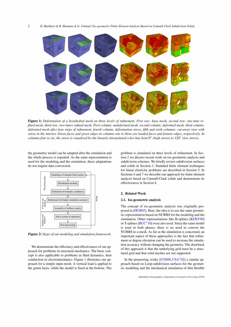
Our method is illustrated in Figure 2. In the initial phasesthe boundary surface is modeled, the interior of the model ismeshed with hexahedra and the boundary conditions, such asexternal forces, are defined. These three steps are regardedas pre-processing and are not discussed in this paper. Theboundary and the interior of the solid model are Catmull-Clark surfaces and Catmull-Clark solids, respectively, withoptional sharp features such as corners and creases. Thus,the solid model is C1-continuous away from the sharp fea-ture in the limit. Subsequently, the solid model can be subdi-vided to increase the accuracy of the simulation. These rulesare simpler than those for NURBS, especially for modelswith arbitrary topology. Next, the stiffness matrices are as-sembled. One obtains a system of equations to be solvedand additional post-processing computations. These last twosteps are the post-processing to our method and are not dis-cussed in this paper. If the simulation results are inadequate

submitted to Eurographics Symposium on Geometry Processing (2010)

2 D. Burkhart & B. Hamann & G. Umlauf / Iso-geometric Finite Element Analysis Based on Catmull-Clark Subdivision Solids

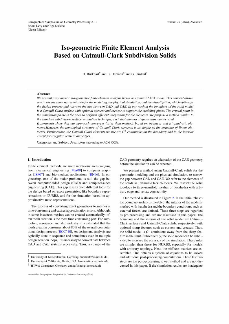
Figure 1: Deformation of a hexahedral mesh on three levels of refinement. First row: base mesh, second row: one-time re-fined mesh, third row: two-times refined mesh. First column: undeformed mesh, second column: deformed mesh, third column:deformed mesh after four steps of refinement, fourth column: deformation stress, fifth and sixth columns: cut-away view withstress in the interior. Green faces and green edges in columns one to three are loaded faces and feature edges, respectively. Incolumns four to six, the stress is visualized by the linearly interpolated color hue from 0 (high stress) to 120 (low stress).

the geometric model can be adapted after the simulation andthe whole process is repeated. As the same representation isused for the modeling and the simulation, these adaptationsdo not require data conversion.

Modeling of Catmull-Clark surface

Hexahedral meshing

Definition of boundary conditions

Refinement for higher simulation accuracy

Assembly of stiffness matrix

Solve system of equations

Post-processing

itera

te

Pre-

proc

essi

ngC

ore

ofou

rm

etho

dSo

lutio

nan

dan

alys

is

Figure 2: Steps of our modeling and simulation framework.

We demonstrate the efficiency and effectiveness of our ap-proach for problems in structural mechanics. The basic con-cept is also applicable to problems in fluid dynamics, heatconduction or electromechanics. Figure 1 illustrates our ap-proach for a simple input mesh. A vertical load is applied tothe green faces, while the model is fixed at the bottom. The

problem is simulated on three levels of refinement. In Sec-tion 2 we discuss recent work on iso-geometric analysis andsubdivision schemes. We briefly review subdivision surfacesand solids in Section 3. Standard finite element techniquesfor linear elasticity problems are described in Section 5. InSections 6 and 7 we describe our approach for finite elementanalysis based on Catmull-Clark solids and demonstrate itseffectiveness in Section 8.

2. Related Work

2.1. Iso-geometric analysis

The concept of iso-geometric analysis was originally pro-posed in [HCB05]. Here, the idea is to use the same geomet-ric representation based on NURBS for the modeling and thesimulation. Other representations like B-splines [KFBY99]or T-splines [BCC∗10] were also used. Since the same modelis used in both phases, there is no need to convert theNURBS to a mesh. As far as the simulation is concerned, animportant aspect of these approaches is the fact that refine-ment or degree elevation can be used to increase the simula-tion accuracy without changing the geometry. The drawbackof this approach is that the underlying grid must be a struc-tured grid and that solid meshes are not supported.

In the pioneering works [COS00, CSA∗02] a similar ap-proach based on Loop-subdivision surfaces for the geomet-ric modeling and the mechanical simulation of thin flexible


D. Burkhart & B. Hamann & G. Umlauf / Iso-geometric Finite Element Analysis Based on Catmull-Clark Subdivision Solids 3

structures is proposed. The subdivision surfaces are used todescribe both, the undeformed geometry and the smooth in-terpolated displacement field with Kirchhoff-Love theory ofthin shells. Due to the usage of subdivision surfaces, this ap-proach supports only unstructured two-manifold meshes.

2.2. Subdivision surfaces

Subdivision surfaces are a a standard modeling tool in com-puter graphics to model free-form surfaces [DKT98]. Theywere first developed in 1978 [CC78, DS78]. A subdivisionsurface is defined as the limit of an iterative refinementprocess, starting with a polygonal base mesh M0 of con-trol points. Iterating the subdivision process generates a se-quence of refined meshes M1, . . . ,Mn, that converges to asmooth limit surface M∞ for n→∞. Usually the subdivi-sion operator can be factored into a topological refinementoperation followed by a geometrical smoothing operation.While the topological refinement inserts new vertices or flipsedges, the geometrical smoothing changes vertex positions.

Subdivision surfaces either approximate or interpolate thebase mesh. For approximating schemes the control pointsof Mi usually do not lie on Mi+1, i ≥ 0. Approximatingschemes for arbitrary quadrangle meshes are Doo-Sabin andCatmull-Clark subdivision [CC78, DS78]. Both are gener-alizations of uniform tensor-product B-spline surfaces. Ap-proximating schemes for arbitrary triangle meshes the algo-rithm of Loop and

√3-subdivision [Loo87, Kob00]. For in-

terpolating schemes all control points of Mi are also in Mi+1,i ≥ 0. Thus, the limit surface interpolates these points. Aninterpolating subdivision scheme for surfaces is the butterflyscheme of [DLG90].

While subdivision surfaces have continuous normals,real-world models have sharp features with discontinuousnormals. To model these features subdivision algorithms aretailored to allow for corners and creases. Examples for suchspecial rules, where tagged edges will yield creases on thesubdivision surface, are presented in [BLZ00,BMZB02]. Formore details on subdivision surfaces we refer to [PR08].

2.3. Subdivision solids

In contrast to subdivision surfaces, subdivision solids havegained much less attention. One of the first algorithms is de-scribed in [JM96, MJ96]. It is a generalization of Catmull-Clark subdivision to 3D solids for smooth deformationsbased on unstructured hexahedral meshes. As the topolog-ical refinement operation of this algorithm made it hard toanalyze the smoothness of the resulting limit solid, a mod-ified operation was proposed in [BSWX02]. The resultingdeformations are provably smooth everywhere except at thevertices of the base mesh.

A subdivision scheme for tetrahedral meshes based ontrivariate box splines was proposed in [CMQ02, CMQ03].

The topological refinement first splits every tetrahedron intofour tetrahedra and one octahedron. Subsequently, every oc-tahedron is split along one of its diagonals into six tetrahedracausing a potential directional bias. To remedy this effectSchaefer et al. [SHW04] use a topological refinement thatsplits the octahedra symmetrically into eight tetrahedra andsix octahedra. Their geometric smoothing allows for glob-ally C2-continuous deformations, except along edges of M0.The major drawback of these schemes is the use of tetrahe-dra and octahedra, which are not well-suited for finite vol-ume simulations, and require a complicated data structure.

A solid subdivision scheme that supports arbitrary poly-hedral elements and adaptive refinement was presented in[Pas02]. However, its topological refinement splits the poly-hedra into pyramids causing complex merging operations inevery subdivision step.

3. Subdivision

3.1. Catmull-Clark surfaces

The subdivision rules for Catmull-Clark surfaces are definedby the following four steps at a vertex of valence n:

1. For each face add a face point to its centroid.2. For each edge add an edge point E = (F0 +2M+F1)/4,

where F0 and F1 are the face points of the two incidentfaces and M is the edge midpoint.

3. For each face connect its face point into all edge points.For quadrilaterals this operation splits each old quadrilat-eral to four new quadrilaterals.

4. Move each original vertex Vold to its new location Vnew =(Favg +2Mavg +(n−3)Vold)/n, where Mavg and Favg arethe averages of all adjacent edge and face points.

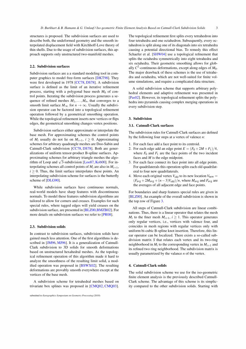
For boundaries and sharp features special rules are given in[BLZ00]. An example of the overall subdivision is shown inthe top row of Figure 3.

All steps of Catmull-Clark subdivision are linear combi-nations. Thus, there is a linear operator that relates the meshMi to the finer mesh Mi+1, i ≥ 1. This operator generatesonly regular vertices, i.e., vertices with valence four, andcoincides in mesh regions with regular vertices only withuniform bi-cubic B-spline knot insertion. Therefore, this lin-ear operator can be localized. There exists a so-called sub-division matrix S that relates each vertex and its two-ringneighborhood in Mi to the corresponding vertex in Mi+1 andits refined two ring neighborhood. The subdivision matrix isusually parametrized by the valance n of the vertex.

4. Catmull-Clark solids

The solid subdivision scheme we use for the iso-geometricfinite element analysis is the previously described Catmull-Clark scheme. The advantage of this scheme is its simplic-ity compared to the other subdivision solids. Starting with



a hexahedral base mesh, only hexahedral elements are gen-erated, all new vertices are regular, i.e. they have six inci-dent edges, and all new edges are regular, i.e. they have fourincident hexahedra. However, this scheme can generate in-verted hexahedra even from a non-self-intersecting hexahe-dral mesh. The subdivision rules for Catmull-Clark solidsfor hexahedral meshes are defined by five steps [JM96]:

1. For each hexahedron add a cell point to its centroid.2. For each face add a face point F = (C0 +2A+C1)/4,

where C0 and C1 are the cell points of the two incidenthexahedra and A is the face centroid.

3. For each edge add an edge point E =(Cavg+ 2Aavg+ (n−3)M)/n, where n is the number of incident faces, M is theedge midpoint, and Cavg and Aavg are the averages of celland face points of incident cells and faces, respectively.

4. For each hexahedron connect its cell point to all its facepoints and connect all its face points to all incident edgepoints. This splits one hexahedron to eight hexahedra.

5. Move each original vertex Vold to its new location Vnew =(Cavg +3Aavg +3Mavg +Vold)/8, where Cavg, Aavg, andMavg are the averages of the cell, face and edge points ofall adjacent cells, faces, and edges.

For faces, edges and vertices on the boundary of the solidcorresponding rules for Catmull-Clark surfaces are applied.An example of this algorithm is shown in Figure 3.

Also for Catmull-Clark solids there is a subdivisionmatrix that relates each vertex and its neighborhood inMi to its corresponding vertex and neighborhood in Mi+1[BSWX02]. However, this matrix depends on the local meshtopology and is thus parametrized via a graph isomorphy.

Figure 3: Two steps of Catmull-Clark refinement applied toa hexahedral mesh with sharp boundary edges (green).

5. Finite element analysis of elastic materials

Finite element analysis is a numerical method to solve partialdifferential equations by discretizing these equations in theirspatial dimensions. This discretization is done locally insmall regions of simple shape (the finite elements) connectedat discrete nodes. The solution of the variational equations is

approximated with local shape functions defined for the fi-nite elements. This results in matrix equations relating theinput (boundary conditions) at the discrete nodes to the out-put at these nodes (the unknown variables). The contributionof each element is computed in terms of local stiffness ma-trices Km, which are assembled into a global stiffness matrixK. This yields for static elasticity problems a linear systemof equations Ku = f, where u is the vector of the unknownvariables and f of the external forces. The computation oflocal stiffness matrices Km depends on the physical problemand is described for linear elastic material in the sequel.

ξ

ηζ

N

x

yz

ξ

ηζ

N

x

yz

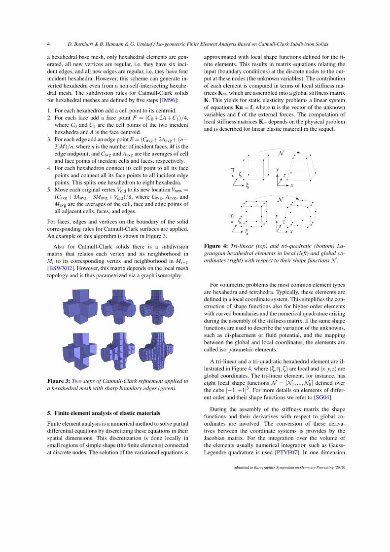
Figure 4: Tri-linear (top) and tri-quadratic (bottom) La-grangian hexahedral elements in local (left) and global co-ordinates (right) with respect to their shape functionsN .

For volumetric problems the most common element typesare hexahedra and tetrahedra. Typically, these elements aredefined in a local coordinate system. This simplifies the con-struction of shape functions also for higher-order elementswith curved boundaries and the numerical quadrature arisingduring the assembly of the stiffness matrix. If the same shapefunctions are used to describe the variation of the unknowns,such as displacement or fluid potential, and the mappingbetween the global and local coordinates, the elements arecalled iso-parametric elements.

A tri-linear and a tri-quadratic hexahedral element are il-lustrated in Figure 4, where (ξ,η,ζ) are local and (x,y,z) areglobal coordinates. The tri-linear element, for instance, haseight local shape functions N = [N1, ...,N8] defined overthe cube [−1,+1]3. For more details on elements of differ-ent order and their shape functions we refer to [SG04].

During the assembly of the stiffness matrix the shapefunctions and their derivatives with respect to global co-ordinates are involved. The conversion of these deriva-tives between the coordinate systems is provides by theJacobian matrix. For the integration over the volume ofthe elements usually numerical integration such as Gauss-Legendre quadrature is used [PTVF07]. In one dimension



these quadrature rules are of the form∫ +1

−1f (x)dx≈

k

∑i=1

wif(xi),

where k is the number of integration points, wi are theweights, and xi are the sampling points. For k = 2 Gauss-Legendre quadrature is exact for cubic polynomials. The val-ues for k = 1,2,3 are shown in Table 1.

k xi wi

1 0 22 −

√1/3 +

√1/3 1 1

3 −√

3/5 0 +√

3/5 5/9 8/9 5/9

Table 1: Sampling points xi and weights wi for Gauss-Legendre quadrature of order k = 1,2,3.

In the theory of linear elasticity, a solid model Ω consistsof a set of nodes x = [x,y,z]T . These nodes are connectedto form the elements for the finite element analysis. Whenforces are applied, Ω is deformed into a new shape. Thus,x is displaced to x + u with u(x) = [u,v,w]T . The bound-ary of the domain Ω consists of the boundary Γ1 with fixeddisplacements u(x) = u0(x), the boundary Γ2 where forcesare applied, and the boundary Γ3 without constraints. Thesecomponents satisfy Γ =

⋃i Γi and

⋂i Γi = ∅.

The strain energy of a linear elastic body Ω is defined as

Estrain =12

∫Ω

εT

σdx,

with the stress vector σ and the strain vector ε =[εx εy εz γxy γxz γyz]

T defined as

εx =∂u∂x

, εy =∂u∂y

, εz =∂u∂z

,

γxy =∂u∂y

+∂v∂x

, γxz =∂u∂z

+∂w∂x

, γyz =∂v∂z

+∂w∂y

.

This can be rewritten as ε = Bu, where B is the so-called strain-displacement matrix, that depends on the partialderivatives of the shape functions of used finite elements

BT =

∂/∂x 0 0 ∂/∂y ∂/∂z 00 ∂/∂y 0 ∂/∂x 0 ∂/∂z0 0 ∂/∂z 0 ∂/∂x ∂/∂y

. (1)

Hooke’s law σ = Cε relates the stress vector σ to ε via thematerial matrix C, which is defined by the Lamé constants λ

and µ. Rewriting the strain energy and adding work appliedby internal and external forces f and g, respectively, yieldsthe total energy function

E(u) = 12

∫Ω

uT BT CBudx−∫

Ω

fT udx−∫

Γ2

gT da. (2)

A detailed discussion is provided in [ZT00, SG04].

6. Assembly of Catmull-Clark solids

We use Catmull-Clark solids for the representation of thegeometry and the approximation of the displacement fielddefined by Equation (2). To solve this equation the finite el-ement method is used to define a linear system of equationsof the form Ku = f, where K is the global stiffness matrix,u is the unknown displacement vector and f are the exter-nal forces. The global stiffness matrix K is defined via theelement stiffness matrices

Km =∫ ∫ ∫

BT CBdxdydz. (3)

As the exact evaluation of (3) is in general not possible,three-dimensional Gauss-Legendre quadrature is used:∫ +1

−1

∫ +1

−1

∫ +1

−1f(x,y,z)dxdydz≈

n

∑i=1

Wif(xi,yi,zi), (4)

where xi, yi and zi are permutations of the sampling pointsof the univariate quadrature rule and Wi is the product of thecorresponding weights. As the elements are defined in localcoordinates, (4) in combination with (3) yields

Km ≈n

∑i=1

Wi det(J)BT CB. (5)

The assembly is illustrated in Procedure 1, where line nineimplements equation (5). In lines two and three the numberof nodes m in the one ring of an element is used to initializethe element stiffness matrix Km. In line six the derivatives Dof the basis functions for the Catmull-Clark elements at thecurrent sampling point p are computed. This function willbe discussed in Section 7.3 in detail. As these derivatives arecomputed in local coordinates ξ,η,ζ, the Jacobian J is com-puted from the global coordinates of the current hexahedronCoordinates(h) (line seven) for the conversion to global co-ordinates x,y,z. Using the Jacobian J and the derivatives D,the strain-displacement matrix B computed in AssembleB(J,D) according to (1). Every part of Procedure 1 can also beused for standard elements except the computation of thederivatives, that is tailored for Catmull-Clark solids.

For standard tri-linear and tri-quadratic elements thesederivatives can be computed directly. For Catmull-Clark el-ements it is not obvious how to compute derivatives due totopologically arbitrary elements as shown in Figure 5(b).However, evaluations of topological arbitrary elements canbe reduced to evaluations of regular elements shown in Fig-ure 5(a). These regular elements can be evaluated directly,see Section 7.1. The evaluation for the irregular elements isdiscussed in Section 7.2. Thus, our approach can be inte-grated with the iso-parametric concept since the same pro-gram code can be used as the one used for the standard finiteelements from Figure 4. Only the evaluation at the samplingpoints needs to be adapted to the arbitrary topological settingillustrated in Figure 5(b).

Once the stiffness matrix K is assembled, the force vector



Procedure 1 AssembleCCElements(HexMesh m)1: for all (HexCC h in m) do2: m = NumberOfNodesInOneRing(h);3: Km = InitMatrix(3 ·m, 3 ·m);4: for (int i = 0; i < n; i++) do5: p = SamplePoint(i);6: D = Derivative(h, p);7: J = D · Coordinates(h);8: B = AssembleB(J, D);9: Km += Wi ·det(J) ·BT ·C ·B; // see (5)

10: end for11: Assemble(K, Km);12: end for

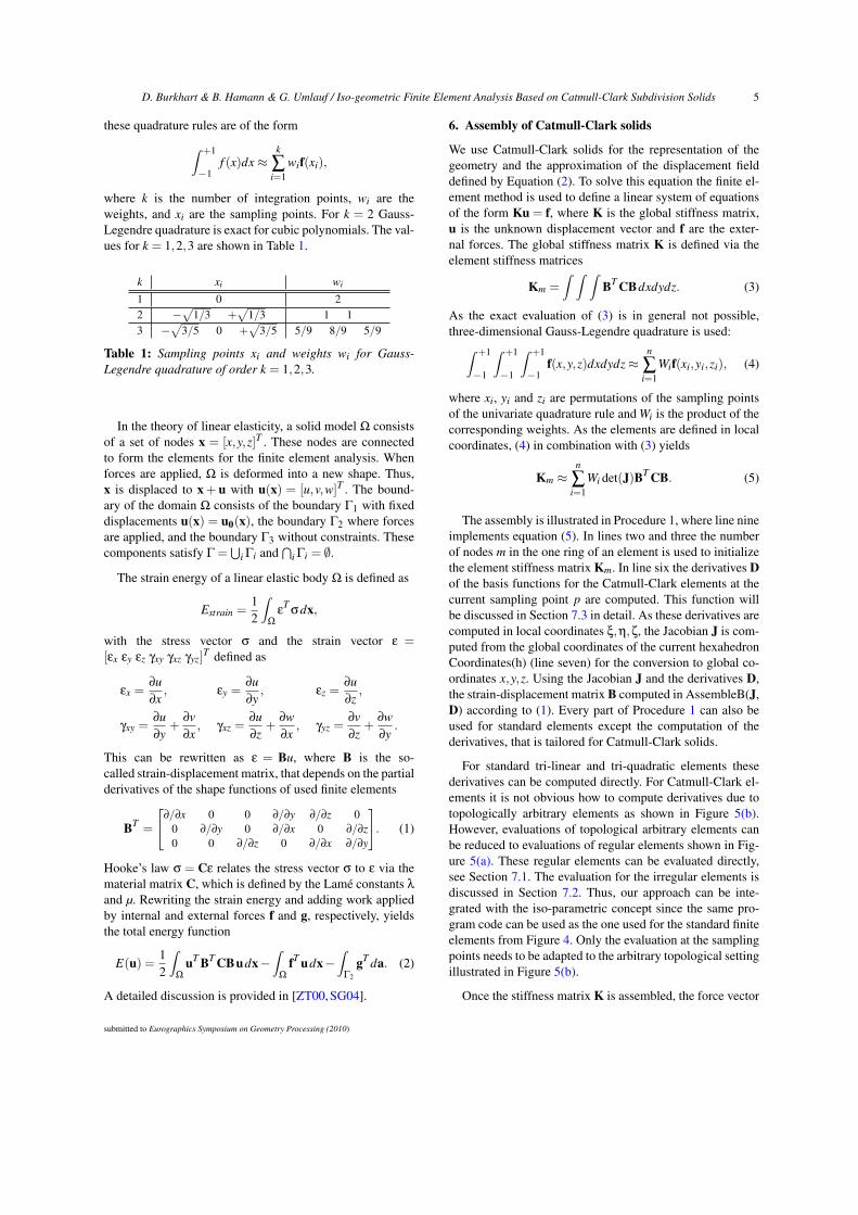
(a) (b)

Figure 5: Regular Catmull-Clark element (left), irregularCatmull-Clark element (right). To evaluate the highlightedhexahedron, all neighbored hexahedra are required.

f can be constructed. Fixed displacements are enforced us-ing the penalty method described in [SG04]. Finally, the lin-ear system of equations Ku = f can be solved with standardlinear solvers. To derive the deformed geometry the com-puted displacement field is applied to the original geome-try. The relation ε = Bue yields the strain at the samplingpoints of the Gauss-Legendre quadrature for each element,where ue is the displacement vector for a single element.With Hooke’s law σ = Cε the stress is computed.

7. Evaluation of Catmull-Clark solids

Using Catmull-Clark solids for finite element analysis, thedisplacement field within an element does not only dependon the displacements of the nodes attached to the element butalso on the displacements of the nodes of adjacent elements,because the support of the basis functions of Catmull-Clarksolids overlaps a one-ring neighborhood of elements. Hence,for the evaluation at the sampling points of the Gauss-Legendre quadrature, the one-ring neighborhood around anelement is required. This is illustrated in Figure 5, where thegray elements are evaluated and all adjacent elements are re-quired for the evaluation.

7.1. The regular case

As Catmull-Clark solids generalize tri-cubic uniform B-splines to arbitrary topology, cubic uniform B-spline ba-sis functions can be used, provided the element has no

irregular vertex, see Figure 5(a). These regular elementsdepend on 64 nodal positions. The associated basis func-tions for (s, t,u) ∈ [0,1]3 and i, j,k = 0, . . . ,3 are given byNi jk(s, t,u) =Ni(s)N j(t)Nk(u), where N0, . . . ,N3 are the uni-form cubic B-spline functions.

7.2. The irregular case

If a hexahedral element has at least one irregular vertex, asshown in Figure 5(b), this technique cannot be applied. How-ever, a technique similar to [Sta98, Sta99] for the evaluationof subdivision surfaces at arbitrary parameter values can beused. This technique is based on the diagonalization of thesubdivision matrix S, where the eigenvectors can be inter-preted as instances of special regular meshes. These can beprecomputed symbolically and evaluated with the B-splineevaluation as discussed in Section 7.1. Thus, iterating thesubdivision process means scaling these special eigenvectormeshes with powers of the corresponding eigenvalues. Thisreduces the evaluation at an arbitrary parameter value to thecomputation of the correct power of the eigenvalue and B-spline evaluations of the tabulated eigenvector meshes.

This technique is not immediately applicable to and re-quired for our application. First, the eigenvectors of thesubdivision matrix are parametrized by a graph isomorphy,which requires the symbolical pre-computation of a largenumber of eigenvectors. Second, for the quadrature rules thesubdivision solids are only evaluated at the sample points.

To evaluate a Catmull-Clark solid at the eight samplepoints of Gauss-Legendre quadrature of order k = 2 usingstandard B-spline evaluation each sample point must lie inthe central element of a regular 3× 3× 3 mesh neighbor-hood. Because one subdivision step bisects the correspond-ing parameter space, after at most ` = 2 subdivisions everysample point of Mi satisfies this requirement in Mi+`. For 27and 64 sample points of Gauss-Legendre quadrature of orderk = 3,4, at most `= 4 subdivision steps are required. This isused to compute the 192 derivatives of the basis functions

ddω

Ni jk(s, t,u), i, j,k ∈ 0, . . . ,3,ω ∈ s, t,u.

Note that the derivatives are scaled by 2−`. Instead of theeigenvectors we pre-compute the evaluation rules.

7.3. Evaluation algorithm

The assembly of Catmull-Clark elements is more expensivethan the assembly of eight-node hexahedral elements for tworeasons. First, eight-node hexahedral elements have 24 de-grees of freedom, while Catmull-Clark elements have in theregular case 192 degrees of freedom. This means that thematrix-matrix multiplications in Equation (3) are more ex-pensive. This can only be handled by a suitable optimizedmatrix library. Second, the computation of the derivativesat the sampling points is more expensive. To optimize this,



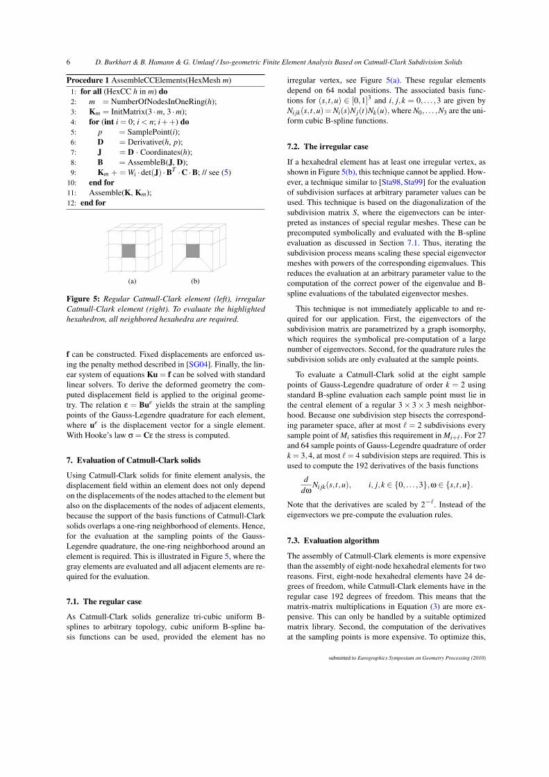
(a) (b)

(c) (d) (e)

Figure 6: Five isomorphy classes for a regular hexahedralmesh with feature edges in red.

we pre-compute and buffer stencils for the derivatives at thesampling points. For all identical one-ring neighborhoodsthe computations have to be done only once.

For regular meshes there is only a small number of iso-morphic one-ring neighborhoods. Five of these are shown inFigure 6. For arbitrary hexahedral meshes it is more complexto determine isomorphic one-ring neighborhoods, since thisis an instance of a graph isomorphism problem [GJ90] whichis NP-complete. Here the valence of an interior vertex doesnot suffice to determine the local mesh topology uniquely.To find isomorphic cases we construct weighted undirectedgraphs of the sub-meshes containing one hexahedron and itsone-ring neighborhood. In the regular case this graph con-sists of 64 nodes and 288 edges. The weights of the edgesof this graph correspond to the tags representing the featuresof the geometric model. For complicated meshes an addi-tional hashing of the graphs avoids many unnecessary graphcomparisons. The hash function we use is

h = 3ne +5nv +7nh +ne

∑i=1

ei, (6)

where ei is the tag of the i-th edge and ne, nv, and nh are thenumber of edges, vertices, and hexahedra in the sub-mesh.

Procedure 2 shows the function to evaluate derivatives ofCatmull-Clark elements at a sampling point p schematically.Here, the matrices D and S represent the derivatives and thesubdivision stencils. The size of D depends on the numberof vertices in the one-ring neighborhood of the hexahedron,which is 3× 192 in the regular case. The irregular meshshown in Figure 5(b) has 48 vertices and D has size 3×144.

In line three the sub-mesh containing the hexahedron tobe evaluated and its one-ring neighborhood are extracted.Then first the isomorphism class of this mesh configura-tion is checked (line five) using the hash function (6). If thismesh configuration is not yet been evaluated, i.e. is not inthe database, the sub-mesh is subdivided (line eight) and theparameters u, v, w are adapted (lines nine to eleven) until the

sampling point lies in a regular sub-mesh. During each stepof refinement the stencil S is adapted too. In line 13 and 14the derivatives for a regular one-ring neighborhood for thecurrent parameters u, v, w and for the original irregular sub-mesh are computed. The function of the stencil S is used tomap the regular subdivided sub-mesh temp to the irregularoriginal sub-mesh sub. Hence, the size of S depends on thenumber of vertices in sub, e.g. for the irregular mesh shownin Figure 5(b) S has the size 192× 144. Finally, the stenciland derivative are stored in a database (line 15).

Procedure 2 Derivative(HexCC h, Point3D p)1: u = p.x; v = p.y; w = p.z;2: level=0;3: sub = SubMesh(h);4: hash = CalcHash(sub);;5: if (D = GetFromDataBase(hash, sub)) return D;6: repeat7: level++;8: temp = Subdivide(sub, S);9: if (u ≤ 0.5) u = 2 ·u; else u = (u −0.5) ·2;

10: if (v ≤ 0.5) v = 2 · v; else v = (v −0.5) ·2;11: if (w≤ 0.5) w = 2 ·w; else w = (w−0.5) ·2;12: until (IsRegular(temp));13: D = EvalBsplineDerivatives(u, v, w);14: D = D ·S ·2−level ;15: SaveToDataBase(hash, sub, D, S);16: return D;

8. Results

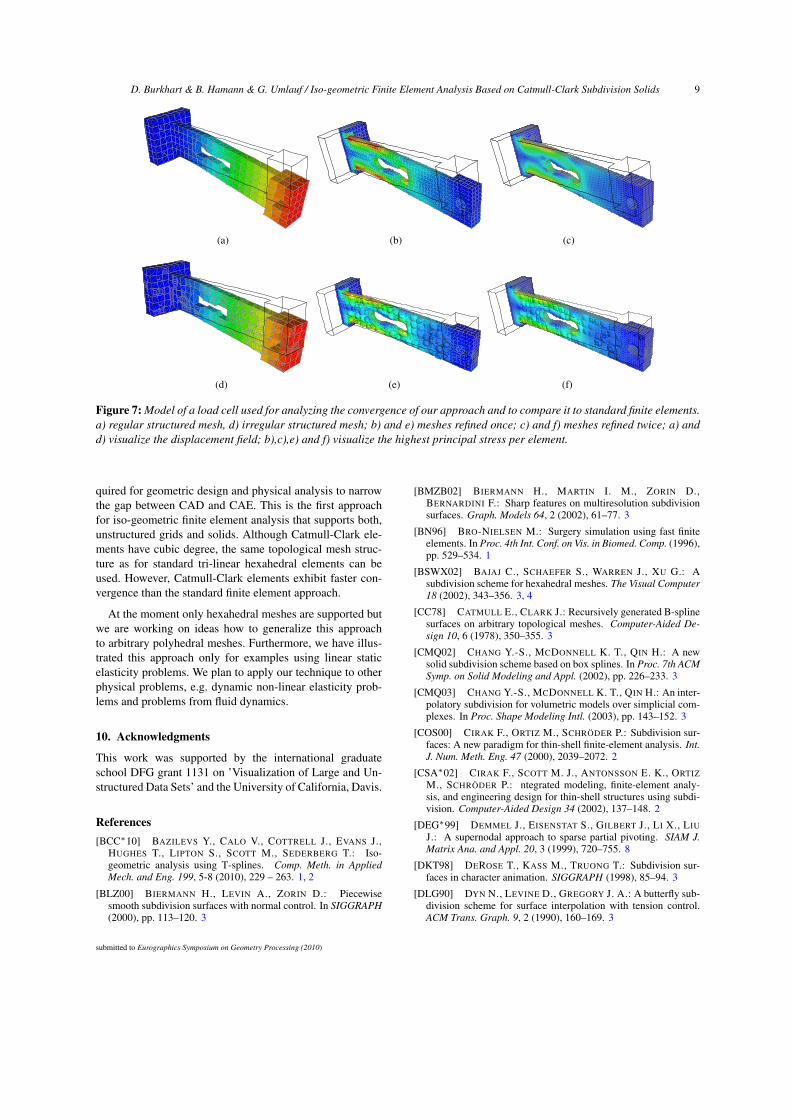
To demonstrate the effectiveness of our approach, we com-pare it to standard finite elements hex8 and hex20 shown inFigure 4. As test case we use the model shown in Figure7(a). This model is fixed at the left side and a vertical loadis applied on the right side. We measure the maximum dis-placement in the direction of the load and compare this dis-placement. For the visualization of the displacement or stressfields we linearly interpolate the color hue from 0 (high dis-placement or stress) to 240 (low displacement or stress).

To show that our approach does not require a regularstructured mesh, we use the unstructured mesh of this modelshown in Figure 7(b). The model in Figure 7(a) consists of221 hexahedra and 504 vertices. The hexahedra are equallysized cubes and vertices and edges are regular, except onboundaries. To generate the model shown in 7(b) we re-fined several hexahedra with an irregular split operation andmoved the vertices randomly. This mesh consists of 800 hex-ahedra and 1,392 vertices. The statistic of irregular verticesand edges in both meshes is shown in Table 2.

To analyze the convergence we subdivide both modelstwice and measure the rate of convergence with respect toa reference solution. The reference solution is the solutioncomputed with hex8 elements on the three times subdivided



Valence Vertices Edges Vertices Edgesin 7(a) in 7(a) in 7(b) in 7(b)

1 0 250 0 1962 0 652 0 10763 16 70 11 16164 172 222 826 3815 244 0 256 616 72 0 104 437 0 0 79 218 0 0 53 14≥9 0 0 63 6

Table 2: Edge and vertex valence for the models shown inFigures 7(a) and 7(a).

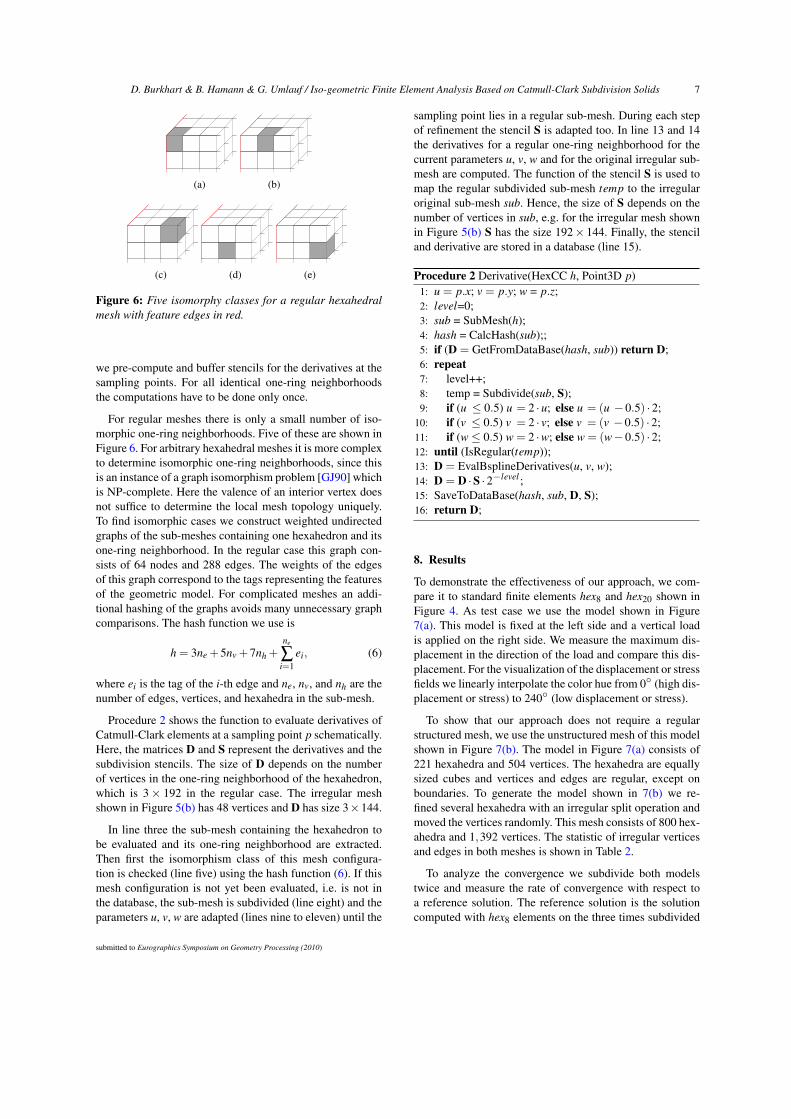
model shown in Figure 7(a), which consists of 113,152 hex-ahedra, 129,059 vertices and hence 387,177 degrees of free-dom. Due to the high number of degrees of freedoms, thereference solution was computed with a conjugate gradientsolver. For all other meshes we assemble the stiffness ma-trices to sparse matrices and use the sparse direct solverSuperLU [DEG∗99]. The line charts shown in Figure 8 il-lustrate the rate of convergence against the normalized er-ror. The timings used in the chart include the assembly ofthe stiffness matrix as described in Procedure 1, solving thelinear system and pre-computing the stresses. For all threetypes of elements the same code is used, except for themethod to compute the derivatives. This method depends onthe finite elements used and is illustrated in Procedure 2 forCatmull-Clark elements. Note that for the computations, thedatabase was pre-computed, such that Procedure 2 for thecomputation of the derivatives of the hexCC elements alwaysterminates in line five.

The reference solution in Figure 8 is the black line atthe normalized maximum displacement of 1. The line chartsshow that Catmull-Clark elements (blue lines) convergefaster than other elements independently of the discretiza-tion (red and green lines). For meshes with the same num-ber of hexahedra, the assembly is fastest for hex8 elementsand slowest for hexCC elements. Solving the linear system ofequations is also fastest with hex8 elements, but hexCC ele-ments are just slightly slower. Solving the linear system ofequations for hex20 elements takes much longer. Althoughthis may depend on the larger number of degrees of free-doms, the overall convergence rate of hex20 elements com-pared to hexCC elements is slower as well.

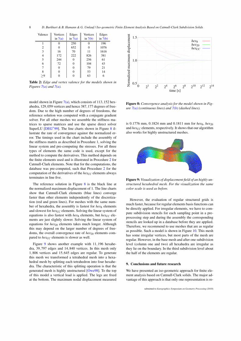
Figure 9 shows another example with 11,196 hexahe-dra, 39,797 edges and 14,840 vertices. In this mesh only1,806 vertices and 15,645 edges are regular. To generatethis mesh we transformed a tetrahedral mesh into a hexa-hedral mesh by splitting each tetrahedron into four hexahe-dra. The characteristic of this splitting operation is that thegenerated mesh is highly unstructured [Owe98]. To the topof this model a vertical load is applied. The legs are fixedat the bottom. The maximum nodal displacement measured

0.5

1.0

1.5

0 21 22 24 26 28 210 212 214

hex8hex20hexCC

time [s]

Nor

mal

ized

max

imum

disp

lace

men

t

Figure 8: Convergence analysis for the model shown in Fig-ure 7(a) (continuous lines) and 7(b) (dashed lines).

is 0.1776 mm, 0.1824 mm and 0.1811 mm for hex8, hex20and hexCC elements, respectively. It shows that our algorithmalso works for highly unstructured meshes.

Figure 9: Visualization of displacement field of an highly un-structured hexahedral mesh. For the visualization the samecolor scale is used as before.

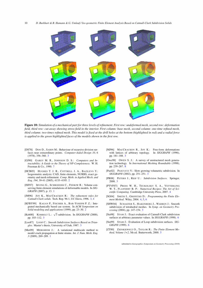
However, the evaluation of regular structured grids ismuch faster, because for regular elements basis functions canbe directly applied. For irregular elements, we have to com-pute subdivision stencils for each sampling point in a pre-processing step and during the assembly the correspondingstencils are looked up in a database before they are applied.Therefore, we recommend to use meshes that are as regularas possible. Such a model is shown in Figure 10. This meshhas some irregular vertices, but most parts of the mesh areregular. However, in the base mesh and after one subdivisionlevel (column one and two) all hexahedra are irregular asthey lie on the boundary. In the third subdivision level aboutthe half of the elements are regular.

9. Conclusions and future research

We have presented an iso-geometric approach for finite ele-ment analysis based on Catmull-Clark solids. The major ad-vantage of this approach is that only one representation is re-



(a) (b) (c)

(d) (e) (f)

Figure 7: Model of a load cell used for analyzing the convergence of our approach and to compare it to standard finite elements.a) regular structured mesh, d) irregular structured mesh; b) and e) meshes refined once; c) and f) meshes refined twice; a) andd) visualize the displacement field; b),c),e) and f) visualize the highest principal stress per element.

quired for geometric design and physical analysis to narrowthe gap between CAD and CAE. This is the first approachfor iso-geometric finite element analysis that supports both,unstructured grids and solids. Although Catmull-Clark ele-ments have cubic degree, the same topological mesh struc-ture as for standard tri-linear hexahedral elements can beused. However, Catmull-Clark elements exhibit faster con-vergence than the standard finite element approach.

At the moment only hexahedral meshes are supported butwe are working on ideas how to generalize this approachto arbitrary polyhedral meshes. Furthermore, we have illus-trated this approach only for examples using linear staticelasticity problems. We plan to apply our technique to otherphysical problems, e.g. dynamic non-linear elasticity prob-lems and problems from fluid dynamics.

10. Acknowledgments

This work was supported by the international graduateschool DFG grant 1131 on ’Visualization of Large and Un-structured Data Sets’ and the University of California, Davis.

References[BCC∗10] BAZILEVS Y., CALO V., COTTRELL J., EVANS J.,

HUGHES T., LIPTON S., SCOTT M., SEDERBERG T.: Iso-geometric analysis using T-splines. Comp. Meth. in AppliedMech. and Eng. 199, 5-8 (2010), 229 – 263. 1, 2

[BLZ00] BIERMANN H., LEVIN A., ZORIN D.: Piecewisesmooth subdivision surfaces with normal control. In SIGGRAPH(2000), pp. 113–120. 3

[BMZB02] BIERMANN H., MARTIN I. M., ZORIN D.,BERNARDINI F.: Sharp features on multiresolution subdivisionsurfaces. Graph. Models 64, 2 (2002), 61–77. 3

[BN96] BRO-NIELSEN M.: Surgery simulation using fast finiteelements. In Proc. 4th Int. Conf. on Vis. in Biomed. Comp. (1996),pp. 529–534. 1

[BSWX02] BAJAJ C., SCHAEFER S., WARREN J., XU G.: Asubdivision scheme for hexahedral meshes. The Visual Computer18 (2002), 343–356. 3, 4

[CC78] CATMULL E., CLARK J.: Recursively generated B-splinesurfaces on arbitrary topological meshes. Computer-Aided De-sign 10, 6 (1978), 350–355. 3

[CMQ02] CHANG Y.-S., MCDONNELL K. T., QIN H.: A newsolid subdivision scheme based on box splines. In Proc. 7th ACMSymp. on Solid Modeling and Appl. (2002), pp. 226–233. 3

[CMQ03] CHANG Y.-S., MCDONNELL K. T., QIN H.: An inter-polatory subdivision for volumetric models over simplicial com-plexes. In Proc. Shape Modeling Intl. (2003), pp. 143–152. 3

[COS00] CIRAK F., ORTIZ M., SCHRÖDER P.: Subdivision sur-faces: A new paradigm for thin-shell finite-element analysis. Int.J. Num. Meth. Eng. 47 (2000), 2039–2072. 2

[CSA∗02] CIRAK F., SCOTT M. J., ANTONSSON E. K., ORTIZM., SCHRÖDER P.: ntegrated modeling, finite-element analy-sis, and engineering design for thin-shell structures using subdi-vision. Computer-Aided Design 34 (2002), 137–148. 2

[DEG∗99] DEMMEL J., EISENSTAT S., GILBERT J., LI X., LIUJ.: A supernodal approach to sparse partial pivoting. SIAM J.Matrix Ana. and Appl. 20, 3 (1999), 720–755. 8

[DKT98] DEROSE T., KASS M., TRUONG T.: Subdivision sur-faces in character animation. SIGGRAPH (1998), 85–94. 3

[DLG90] DYN N., LEVINE D., GREGORY J. A.: A butterfly sub-division scheme for surface interpolation with tension control.ACM Trans. Graph. 9, 2 (1990), 160–169. 3



Figure 10: Simulation of a mechanical part for three levels of refinement. First row: undeformed mesh, second row: deformationfield, third row: cut-away showing stress field in the interior. First column: base mesh, second column: one-time refined mesh,third column: two-times refined mesh. This model is fixed at the drill holes at the bottom (highlighted in red) and a radial forceis applied to the green highlighted faces of the models shown in the first row.

[DS78] DOO D., SABIN M.: Behaviour of recursive division sur-faces near extraordinary points. Computer-Aided Design 10, 6(1978), 356–360. 3

[GJ90] GAREY M. R., JOHNSON D. S.: Computers and In-tractability; A Guide to the Theory of NP-Completeness. W. H.Freeman & Co., 1990. 7

[HCB05] HUGHES T. J. R., COTTRELL J. A., BAZILEVS Y.:Isogeometric analysis: CAD, finite elements, NURBS, exact ge-ometry and mesh refinement. Comp. Meth. in Applied Mech. andEng. 194, 39-41 (2005), 4135–4195. 2

[ISF07] IRVING G., SCHROEDER C., FEDKIW R.: Volume con-serving finite element simulations of deformable models. In SIG-GRAPH (2007), p. 13. 1

[JM96] JOY K., MACCRACKEN R.: The refinement rules forCatmull-Clark solids. Tech. Rep. 96-1, UC Davis, 1996. 3, 4

[KFBY99] KAGAN P., FISCHER A., BAR-YOSEPH P. Z.: Inte-grated mechanically based cae system. In ACM Symposium onSolid modeling and applications (1999), pp. 23–30. 2

[Kob00] KOBBELT L.:√

3 subdivision. In SIGGRAPH (2000),pp. 103–112. 3

[Loo87] LOOP C.: Smooth Subdivision Surfaces Based on Trian-gles. Master’s thesis, University of Utah, 1987. 3

[Mer09] MERGHEIM J.: A variational multiscale method tomodel crack propagation at finite strains. Int. J. Num. Meth. Eng.3 (2009), 269–289. 1

[MJ96] MACCRACKEN R., JOY K.: Free-form deformationswith lattices of arbitrary topology. In SIGGRAPH (1996),pp. 181–188. 3

[Owe98] OWEN S. J.: A survey of unstructured mesh genera-tion technology. In International Meshing Roundtable (1998),pp. 239–267. 8

[Pas02] PASCUCCI V.: Slow growing volumetric subdivision. InSIGGRAPH (2002), pp. 251–251. 3

[PR08] PETERS J., REIF U.: Subdivision Surfaces. Springer,2008. 3

[PTVF07] PRESS W. H., TEUKOLSKY S. A., VETTERLINGW. T., FLANNERY B. P.: Numerical Recipes: The Art of Sci-entific Computing. Cambridge University Press, 2007. 4

[SG04] SMITH I., GRIFFITHS D.: Programming the Finite Ele-ment Method. Wiley, 2004. 4, 5, 6

[SHW04] SCHAEFER S., HAKENBERG J., WARREN J.: Smoothsubdivision of tetrahedral meshes. In Symp. on Geometry Pro-cessing (2004), pp. 147–154. 3

[Sta98] STAM J.: Exact evaluation of Catmull-Clark subdivisionsurfaces at arbitrary parameter values. In SIGGRAPH (1998). 6

[Sta99] STAM J.: Evaluation of Loop subdivision surfaces. SIG-GRAPH (1999). 6

[ZT00] ZIENKIEWICZ O., TAYLOR R.: The Finite Element Me-thod, Volume 1+2, 5th ed. Butterworth, 2000. 5


iso-geometric finite element analysis based on...

Documents