isosurfaces and level-setsurface models
TRANSCRIPT

Isosurfacesand Level-SetSurfaceModelsTutorial Notes1
RossT. Whitak erScientific Computing and Imaging Institute
Schoolof ComputingUniversity of Utah
1 Intr oduction
1.1 Moti vation
Thesenotes addressmechanismsfor analyzing andprocessingvolumesin a way thatdealsspecificallywith isosur-faces. The underlying philosophy is to useisosurfacesas a modeling technology that canserve as an alternativeto parameterizedmodels for a varietyof important applications in visualizationandcomputer graphics. This paperpresentsthemathematicsandnumerical techniquesfor describingthegeometryof isosurfacesandmanipulatingtheirshapesin prescribed ways. We startwith a basicintroduction into the notationandfundamentalconcepts andthenpresentsthegeometryof isosurfaces.We describethemethodof level sets,i.e., moving isosurfaces,andpresent themathematicalandnumericalmethods they entail.Thispaperconcludeswith someapplicationexamplesanddescribesVISPACK, aC++, object-orientedlibrary theperformsvolume processingandlevel-setmodeling.
1.2 Isosurfaces
1.2.1 Modeling SurfacesWith Volumes
Whenconsidering surfacemodelsfor graphics andvisualization,oneis facedwith a staggering variety of optionsincluding meshes,spline-basedpatches,constructive solid geometry, implicit blobs, and particle systems. Theseoptionscanbedividedinto two basicclasses— explicit (parameterized)modelsandimplicit models.With animplicitmodel, onespecifiesthemodel asa level setof ascalarfunction,����� ���� ��� ���� � � (1)
where����� ��
is thedomainof thevolume(andtherangeof thesurfacemodel). Thus,asurface� is
������� � �"! �$#%� �'&%( (2)
Thechoiceof � is arbitrary, and�
is sometimes calledtheembedding. Noticethatsurfacesdefinedin this way divide�into aclearinsideandoutside—suchsurfaces arealwaysclosedwherever they donot intersecttheboundaryof the
domain.Choosing this implicit strategy begs thequestionof how to represent
�. Historically, implicit models arerepre-
sentedusinglinearcombinationsof basisfunctions.Thesebasisor potential functionsusuallyhaveseveraldegreesoffreedom including 3D position, size,andorientation. By combining thesefunctions,onecancreatecomplex objects.Typical modelsmightcontainseveralhundredto several thousandsof suchprimitives. This is thestrategy behind the“blobby” modelsproposedby Blinn [1].
While suchan implicit modeling strategy offers a variety of new modeling tools, it hassomelimitations. Inparticular, theglobal natureof thepotential functionslimits onesability to model localsurfacedeformations. Considerapoint �*)+� where� is thelevel surfaceassociatedwith amodel
� �-,/.10 . , and 0 . is oneof theindividualpotentialfunctions thatcomprise thatmodel. Supposeonewishesto move thesurfaceat thepoint � in a way thatmaintainscontinuity with the surrounding neighborhood. With multiple, global basisfunctionsonemustdecidewhich basisfunction or combination of basisfunctions to alter and at the sametime control the effects on other partsof thesurface.Theproblemis generally ill posed— therearemany waysto adjustthebasisfunctionssothat � will move in
1Versionsof thesenotesandtheaccompanying talk appearedin tutorialsat IEEEVisualization 2000and2001,andACM SIGGRAPH2001.

x
φ
Basis function
k
Figure 1: A volumecanbeconsideredasanimplicit model with a largenumber of localbasisfunctions.
thedesireddirection andyet it maybeimpossibleto eliminatetheeffectsof thosemovementson otherdisjoint partsof the surface. Theseproblemscanbe overcome,however they usuallyentail heuristics that tie the behavior of thesurfacedeformationto thechoiceof representation[2].
An alternative to usinga smallnumber of global basisfunctionsis to usea relatively largenumber of local basisfunctions. This is theprinciplebehind usinga volume asan implicit model. A volumeis a discretesamplingof theembedding
�. It is alsoanimplicit model with a very largenumberof basisfunctions,asshown in Figure1. Thetotal
numberof basisfunctionsis fixed,asaretheirpositions(gridpoints)andextent.Onecanchangeonly themagnitudeofeachbasisfunction, i.e.,eachbasisfunctionhasonly onedegreeof freedom. A typicalvolumeof size 243157682�315 692�3:5contains over a million suchbasisfunctions. Theshapeof eachbasisfunction is opento interpretation— it dependson how oneinterpolatesthe valuesbetweenthe grid points. A trilinear interpolation, for instance,implies a basisfunction thatis apiece-wisecubic polynomialwith avalueof oneat thegrid pointandzeroatneighboring grid points.Another advantageof usingvolumesasimplicit models,is that for thepurposesof analysiswe cantreatthevolumeasa continuous function whosevaluescanbe setat eachpoint according to the application. Oncethe continuousanalysisis completewecanmapthealgorithm into thediscretedomainusingstandardmethodsof numericalanalysis.Thesectionsthatfollow discusshow to computethegeometryof surfacesthatarerepresentedasvolumesandhow tomanipulatetheshapesof thosesurfacesby changing thegray-scalevaluesin thevolume.
1.2.2 IsosurfaceExtraction and Visualization
This paperaddressesthequestionof how to usevolumesassurfacemodels.Depending on theapplication, however,a 3D grid of data(i.e. a volume)may not be a suitablemodel representation. For instance,if the goal is makemeasurementsof anobjector visualizeits shape,anexplicit model might benecessary. In suchcasesit is beneficialto convert betweenvolumesandothermodeling technologies.
For instance,theliteratureproposesseveralmethods for scanconvertingpolygonalmeshesor solidmodels[3, 4].Likewiseavarietyof methodsexist for extractingparametricmodelsof isosurfacesfrom volumes. Themostprevalentmethodis to locateisosurfacecrossingsalonggrid linesin a volume(betweenvoxelsalongthe3 cardinal directions)

andthento link thesepointstogether to form trianglesandmeshes.This is thestrategy of “marching cubes”[5] andotherrelatedapproaches.However, extracting a parametric surfaceis not essentialfor visualization, anda varietyofdirectmethods[6, 7] arenow computationally feasibleandarguably superior in quality. Thesenotesdo not addresstheissueof extracting or renderingisosurfaces,but ratherstudiesthegeometryof isosurfacesandhow to manipulatethemdirectly by changing thegrey-scalevaluesin theunderlyingvolume. Thus,weproposevolumesasamechanismfor studyinganddeforming surfaces,regardlessof theultimateform of theoutput.Theiraremany waysof renderingor visualizingthemandandthesetechniquesarebeyond thescopeof this discussion.
2 SurfaceNormals
Thesurfacenormal of anisosurfaceis givenby thenormalizedgradient vector. Typically, weidentifyasurfacenormalwith a point in thevolumedomain; . Thatis
< ! �%#%� = �"! �%#� = �"! �%#>� where ��)�; ( (3)
Theconventionregarding thedirectionof this vectoris arbitrary; thenegative of thenormalized gradient magnitudeis alsonormal to theisosurface.Thegradient vector points towardthatsideof theisosurfacewhichhasgreatervalues(i.e. brighter).Whenrendering, theconventionis to useoutwardpointing normals,andthesignof thegradient mustbeadjustedaccordingly. However, for mostapplicationsany consistentchoiceof normal vectorwill suffice.Onadiscretegrid, onemustalsodecidehow to approximatethegradient vector(i.e.,first partialderivatives).In many casescentraldifferenceswill suffice. However, in thepresenceof noise,especiallywhenvolumerendering, it is sometimeshelpfulto compute first derivativesusingsomesmoothing filter (e.g., convolution with a Gaussian).Whenusingthenormalvectorto solve certainkinds of partial differential equations, it is sometimesnecessaryto approximatethe gradientvectorwith discrete,one-sideddifferences,asdiscussedin successivesections.
Notethata singlevolumecontainsfamiliesnestedisosurfaces,arranged like the layersof anonion. We specificthenormal to anisosurfaceasa functionof thepositionwithin thevolume. Thatis, < ! �%# is thenormal of the(single)isosurfacethatpassesthroughthepoint � . The � valueassociatedwith thatisosurfaceis
�"! �%# .3 Second-Order Structur e
In differentialgeometric terms,thesecond-orderstructureof asurfaceis characterizedby aquadraticpatchthatsharesfirst- andsecond-ordercontactwith the surfaceat a point (i.e., tangent planeandosculatingcircles). The principaldirectionsof thesurfacearethoseassociatedwith thequadraticapproximation, andtheprincipal curvatures, �7?:�@�BA ,arethecurvaturesin thosedirections.
Thesecond-structureof the isosurfacecanbecomputedfrom thefirst- andsecond-order structureof theembed-ding,
�. All of the isosurface shapeinformationis contained field of normalsgiven by < ! �%# . The C+6DC matrix of
derivativesof this vector, E �GFIH < J�< KI< LNM (4)
describesthesecond-order structureof thesurface.This matrix has(typically) ranktwo, andthetwo nonzeroeigen-valuesof thismatrixgive theprinciplecurvatures.Thatis,O1? � �P?1��O�A � �QA1�RO � �/S ( (5)
Themeancurvature is themeanof thetwo principal curvatures,which is onehalf of thetraceofE ! �%# [8]:T � �P?%U��BA3 � 23 V�W !YX #� � AJ !Y� KZK7U � L@L # U � AK ![� JNJ\U � L@L # U � AL !Y� JNJ]U � KZK #"FI3 � J � K � J4K FI3 � J � L � J4L F^3 � K � L � KZL3 !Y� AJ U � AK U � AL # �R_ A (6)

TheGaussiancurvature is theproductof theprincipalcurvatures:` � � ? � A � O ? O A UaO ? O � U*O A O � �/3 VbW !cX # A F 23 �d� X �e� (7)
�� AL !Y� JNJ � KZK F � J4K � J4K # U � AK !Y� JNJ � LRL F � J4L � J4L # U � AJ !Y� KZK � L@L F � KZL � K>L #U 3 ![� J � K !Y� JNL � KZL F � J4K � L@L # U � J � L !Y� JNK � KZL F � J4L � KZK # U � K � L !Y� JNK � J4L F � KZL � J4J #�#!Y� AJ U � AK U � AL # A (
Thetotalcurvature,alsocalledthedeviationfromflatness,; , is therootsumof squaresof thetwoprincipal curvatures,which is theEuclidean norm of thematrix
E.
Notice, thesemeasuresexist at every point in�
, andat eachpoint they describethe geometry of the particularisosurfacethat passesthrough that point. All of thesequantitiescanbecomputed on a discretevolume usingfinitedifferences,asdescribedin successivesections.
4 Deformable Surfaces
This sectionbegins with mathematics for describing surfacedeformationson parametric models. The result is anevolution equation for a surface. Eachof the termsin this evolution equation canbe re-expressedin a way that isindependentof theparameterization.Finally, theevolution equationfor aparametricsurfacegives riseto anevolutionequation (differentialequation) ona volume,whichencodestheshapeof thatsurfaceasa level set.
4.1 SurfaceDeformation
A regularsurface� �f� � is a collectionof points in 3D thatcanbeberepresented locally asa continuousfunction.In geometric modeling a surfaceis typically representedasa two-parameterobjectin a three-dimensional space,i.e.,a surfaceis local amapping g : g ��h 6 hI�� � ��i j b�� ���� � (8)
whereh 6 hk� A , andthe bold notationrefers specificallyto a parameterizedsurface(vector-valuedfunction). A
deformablesurfaceexhibits somemotion over time. Thus g��lg ! i:�RjQ��m # , where m ) � on. We assumesecond-
order-continuous,orientable surfaces;therefore at every point on the surface(andin time) thereis surfacenormalp � p ! i:�RjQ��m # . We use�rq to referto theentiresetof pointson thesurface.Local deformationsof g canbedescribedby anevolution equation, i.e., a differentialequationon g that incor-
porates thepositionof thesurface,local andglobalshapeproperties,andresponsesto otherforcing functions. Thatis, s gs m �ut ! g � g v � g�w � g v�v � g v@w � g�wxw �>(N(>( # � (9)
wherethesubscriptsrepresent partialderivativeswith respectto thoseparameters.Theevolution of g canbedescribedby asumof termsthatdependsonboththegeometry of g andtheinfluence of otherfunctions or data.
There area varietyof differential expressionsthat canbecombined for different applications. For instance,themodel couldmove in responseto somedirectional “forcing” function[9, 10], y �z������ �
, thatiss gs m �/y ! g7# ( (10)
Alternatively, thesurfacecouldexpandandcontractwith a spatially-varying speed.For instance,s gs m �|{ ! g7# p (11)
where { �P� � ��}� is a signedspeedfunction. Theevolution might alsodepend on thesurfacegeometryitself. For
instance, s gs m �~g vRv U g wxw (12)

Figure2: Level-setmodelsrepresent curvesandsurfacesimplicitly usinggreyscaleimages:a)anellipseis representedasthelevel setof animage,b) to changetheshapewemodify thegreyscalevaluesof theimage.
describesa surface that movesin way that is becomes more smoothwith respectto its own parameterization.Thismotioncanbecombinedwith themotionof Equation 10 to producea model that is pushedby a forcing function butmaintainsa certainsmoothnessin its shapeandparameterization.Therearemyriad termsthat depend on both thedifferentialgeometryof thesurfaceandoutsideforcesor functions to controltheevolution of a surface.
5 Deformation: The Level SetApproach
Themethod of level-sets,proposedby OsherandSethian[11] anddescribedextensively in [8], providesthemathe-maticalandnumerical mechanismsfor computing surfacedeformationsastime-varying iso-valuesof
�by solvinga
partialdifferentialequation on the3D grid. Thatis, thelevel-setformulationprovidesa setof numerical methodsthatdescribehow to manipulatethegreyscalevaluesin avolume, sothattheisosurfacesof
�movein aprescribedmanner
(shown in Figure2).We denotethemovementof a point on a surfaceasit deformsas �����:� m , andwe assumethat this motioncanbe
expressedin termsof the positionof ��) �andthe geometry of the surfaceat that point. In this case,thereare
generally two options for representingsuchsurfacemovementsimplicitly:
Static: A single,static�"! ��# containsa family of level setscorrespondingto surfacesasdifferent times m . Thatis,�"! � ! m #�#�� � ! m #�� = �"! ��#�� s �m � � � ! m #� m ( (13)
Tosolvethisstaticmethod requiresconstructinga�
thatsatisfiesequation13.Thisis aboundaryvalueproblem,which can be solved somewhat efficiently startingwith a single surfaceusing the fast marching methodofSethian[12]. This representationhassomesignificantlimitations, however, because(by definition) a surfacecannot passbackover itself over time, i.e.,motionsmustbestrictly monotonic — inwardor outward.
Dynamic: Theapproachis to usea one-parameter familyof embeddings,i.e.,�"! � ��m # changesover time, � remains
on the � level setof�
asit moves,and � remainsconstant. Thebehavior of�
is obtainedby settingthe total

derivativeof�"! � ! m # ��m #�� � to zero. Thus,�"! � ! m # ��m #�� � � s �s m ��F = � � ���� m ( (14)
This approachcanaccommodatemodelsthatmove forward andbackward andcrossbackover their own paths(over time). However, to solve this requiressolvingtheinitial valueproblem (usingfinite forward differences)on�"! � ��m # — apotentially largecomputationalburden. Theremainderof thisdiscussionfocusesonthedynamic
case,becauseof its superior flexibility .
All surfacemovementsdepend on positionandgeometry, andthelevel-setgeometry is expressedin termsof thedifferential structureof
�. Therefore the dynamic formulation from equation 14 givesa general form of the partial
differentialequationon�: s �s m ��F = � � ���� m �GF = � �4y ! � ��� � ��� A � �>(N(>( # � (15)
where;+� � is thesetof order- � derivativesof�
evaluatedat � . Becausethis relationship appliesto every level-setof�, i.e. all valuesof � , thisequationcanbeappliedto all of
�, andtherefore themovementsof all thelevel-setsurfaces
embeddedin�
canbecalculatedfrom Equation 15.Thelevel-setrepresentationhasanumberof practicalandtheoreticaladvantagesoverconventionalsurfacemodels,
especiallyin thecontext of deformationandsegmentation. First, level-setmodelsaretopologically flexible, they caneasily representcomplicatedsurfaceshapesthat can, in turn, form holes,split to form multiple objects,or mergewith otherobjectsto form a singlestructure. Thesemodels canincorporatemany (millions) of degreesof freedom,andtherefore they canaccommodatecomplex shapes.Indeed,theshapesformedby thelevel setsof
�arerestricted
only by theresolution of thesampling.Thus,thereis no needto reparameterizethemodel asit undergoessignificantdeformations.
Suchlevel-set methods are well documentedin the literature [11, 13] for applications suchas computationalphysics [14], imageprocessing[15, 16], computer vision [17, 18], medicalimageanalysis [19, 18], and3D recon-struction[20, 21]. For instance,in computationalphysicslevel-setmethodsareaapowerful tool for modeling movinginterfacesbetweendifferentmaterials(seeOsherandFedkiw[14] for aniceoverview of recent results).Examplesarewater-air andwater-oil. In suchcases,level-setmethodscanbeusedto compute deformationsthatminimize surfaceareawhile preserving volumesfor materialsthatsplit andmerge in arbitraryways. Themethodcanbeextended tomultiple,non-overlappingobjects.
Level-setmethodshavealsobeenshowntobeeffectivein extractingsurfacestructuresfrombiologicalandmedicaldata. For instanceMalladi et al. [18] proposea method in which the level-setsform an expandingor contractingcontourwhichtendsto “cling” to interestingfeaturesin 2Dangiograms.At thesametimethecontour is alsoinfluencedby its own curvature,and therefore remainssmooth. Whitaker et al. [19, 22] have shown that level setscanbeusedto simulateconventional deformablesurfacemodels,anddemonstratedthis by extracting skin andtumors fromthick-sliced(e.g. clinical) MR data,andby reconstructinga fetal facefrom 3D ultrasound. A variety of authors[23, 24, 16, 25] have presentedvariations on themethodandpresentedresultsfor 2D and3D data.Sethian[8] givesseveralexamplesof level-setcurves andsurfacefor segmenting CT andMR data.
5.1 Deformation Modes
In the caseof parametric surfaces,onecanchoosefrom a variety of different expressionsto construct an evolutionequation thatis appropriatefor aparticularapplication. Foreachof thoseparametricexpressions,thereis acorrespond-ing expressionthatcanbeformulatedon
�, thevolumein which thelevel-setmodelsareembedded.In constructing
evolutions on levels sets,therecanbe no reference to theunderlying surfaceparameterization(termsdependingoni and j in Equations8 through 12). This hastwo important implications: 1) only thosesurfacemovementsthatarenormal to thesurfacearerepresented—any othermovementis equivalent to a reparameterization2) all of thederiva-tiveswith respectto surfaceparameters i and j mustbeexpressedin termsof invariantsurfacepropertiesthatcanbederived withouta parameterization.
Considertheterm g vRv U g wxw from equation12. If i:�Rj is anorthonormalparameterization, theeffect of thattermisbasedpurely onsurfaceshape,notontheparameterization,andtheexpression g vRv U g wxw is twice themeancurvature,H, of thesurface. Thecorresponding level-setformulation is givenby Equation 6.
Table1showsalist of expressionsusedin theevolutionof parameterizedsurfacesandtheirequivalentsfor level-setrepresentations.Also given aretheassumptions abouttheparameterizationthatgiveriseto thelevel-setexpressions.

Effect Parametric EvolutionLevel-SetEvolution
ParameterAssumptions
1 External force y y�� = � None
2Expansion/contraction
{ ! �%# p { ! ��#>� = �"! � ��m #>� None
3Mean
curvature� v�v U � wxw T � = � � Orthonormal
4Gauss
curvature� v�v]6 � wxw ` � = � � Orthonormal
5 Secondorder� vRv or
� wxw � T���� T A F `�� � = � � Principalcurvatures
Table1: A list of evolution termsfor parametric models hasa corresponding expressionon theembedding,�, associ-
atedwith thelevel-setmodels.
6 Numerical Methods
By takingthestrategy of embeddingsurfacemodelsin volumes,we haveconvertedequationsthatdescribe themove-mentof surfacepointsto nonlinear, partialdifferentialequationsdefinedona volume,which is generally a rectilineargrid. The expression�"�.�� �R� � refersto the � th time stepat position � �[�Q�R� , which hasan associatedvalue in the 3Ddomain of thecontinuousvolume
��! . �� � ��� � # . Thegoalis to solve thedifferentialequationconsistingof termsfromTable5.1onthediscretegrid ���.c� ��� � .
Thediscretizationof theseequationsraisestwo important issues.First is the availability of accurate,stablenu-mericalschemesfor solvingtheseequations.Secondis theproblem of computationalcomplexity andthefactthatwehave converteda surfaceproblemto a volumeproblem, increasingthedimensionality of thedomainover which theevolution equationsmustbesolved.
Thelevel-settermsin Table1 arecombined,basedon theneedsof theapplication, to createa partialdifferentialequation on
�"! � ��m # . The solutionsto theseequations arecomputedusingfinite differences. Along the time axissolutionsareobtained usingfinite forward differences,beginning with an initial model (i.e., volume)andsteppingsequentiallythroughaseriesof discretetimessteps(whicharedenotedassuperscriptson � ). Thustheupdateequationis: � � n ?.�� �R� ���|� �.�� �R� � U���m�� � �.c� ��� � � (16)
Theterm � �r�.�� �R� � is a discreteapproximationtos � � s m , which consistsof a weightedsumof termssuchasthosein
Table5.1.Thosetermsmust,in turn, beapproximatedusingfinite differenceson thevolume grid.
6.1 Up-wind Schemes
The termsin Table1 fall into two basiccategories: thefirst-orderterms(items1 and2 in Table1) andthe second-orderterms(items3 through 5). The first-ordertermsdescribe a moving wave front with a space-varying velocity(expression1) or speed(expression2). Equationsof this form cannotbesolvedwith asimplefinite forwarddifferencescheme.Suchschemestendto overshoot,andthey areunstable. To addressthis issueOsherandSethian[26] haveproposedanup-windscheme.Theup-windmethodreliesonaone-sidedderivative thatlooks in theup-wind directionof themoving wave front, andtherebyavoidstheover-shootingassociatedwith finite forward differences.
We denotethetypeof discretedifferenceusingsuperscripts on a differenceoperator, i.e., � � nr� for forwarddiffer-ences,�P�� � for backwarddifferences,and � for centraldifferences.For instance,differencesin the direction on adiscretegrid, � .c� ��� � , with domain ¡ anduniform spacing¢ aredefinedas
� � nr�J � .�� �R� � £� ! � . n ? � �R� � F�� .�� �R� � #��B¢ � (17)� �� �J � .�� �R� � £� ! � .c� ��� � F�� . ? � ��� � #R�1¢ � and (18)� J � .�� �R� � £� ! � . n ? � �R� � F�� . ? � �R� � #�� ! 3Q¢¤# � (19)
(20)

Level-set motion
xi
ui
∆ui
Up-wind difference
Down-wind difference
Down wind Up wind
xi
ui
∆t∆ui limited by up-wind difference
Overshoot creates“new” level sets
Figure3: Theup-windnumerical schemeusesone-sidedderivativesto preventovershootingandthecreationof newlevel sets.
wherewehaveleft off thetimesuperscript for conciseness.Second-ordertermsarecomputedusingthetightest-fittingcentraldifferenceoperators.For example,
� J4J � .c� ��� � £� ! � . n ? � ��� � U � . ? � ��� � F^31� .c� ��� � #¤�1¢ A � (21)� L@L � .c� ��� � £� ! � .c� ��� � n ? U � .c� ��� � ? F^31� .c� ��� � #¤�1¢ A � and (22)� JNK � .c� ��� � £� � J � K � .�� �R� � (23)
Thediscreteapproximationto thefirst-order termsof in Table5.1 arecomputedusingtheup-wind proposedbyOsherandSethian[11]. This strategy avoids overshootingby approximating the gradient of
�usinga one-sided
differencesin thedirection that is up-windof themoving level-setthereby ensuring thatno new contours arecreatedin theprocessof updating �¥�.c� ��� � (asdepictedin Figure3). Theschemeis separablealongeachaxis(i.e., , , and � ).
ConsiderTerm1 in Table5.1. If weusesuperscripts to denotethevector components,i.e.,y ! ��� ���� #%� !c¦ � J � ! ��� ���� # � ¦ � K � ! ��� ���� # � ¦ � L � ! b�� ���� #�# � (24)
theup-wind calculation for a grid point �$�.�� �R� � is
y ! . �� . ��� . #¥� = �"! . �� � �R� � ��m #%§ ¨©@ªz« J � K � L¬ ¦ � © � ! . �� . ��� . #"® � n© �'�.c� ��� � ¦ � © � ! . �� . �R� . #°¯�S� .© ���.c� ��� � ¦ � © � ! . �� . �R� . #°±�S (25)
Thetimestepsarelimited—thefastestmoving wave front canmoveonly onegrid unit periteration.Thatis��m y³² 2,/©@ªz« J � K � LZ¬µ´�¶�· .c� ��� � ªB¸ �P� = ¦ � © � ! . �� � �R� � #>� & ( (26)
ForTerm2 in Table5.1thedirection of themoving surfacedependsonthenormal, andthereforethesameup-windstrategy is appliedin a slightly differentform.{ ! . �� � ��� � #N� = �"! . �� � ��� � ��m #>�B§
¨©ªz« J � K � LZ¬ { ! . �� . ��� . # ®-¹9º1» A ! � n© �'�.c� ��� � � SQ# U ¹8¼d½ A ! �z © ���.c� ��� � � SQ#¾{ ! . �� . �R� . #¿¯ÀS¹8¼d½ A ! � n© ���.�� �R� � � Sz# U ¹Áº1» A ! �z © ���.c� ��� � � SQ#¾{ !c # ! . �� . �R� . #°±�S (27)
Thetimestepsare,again, limited by thefastestmoving wave front:��mxà ² 2C ´�¶�· .c� ��� � ªB¸ �P� = { ! . �� � ��� � #>� & (28)

Figure4: A level curve of a 2D scalarfield passesthrough a finite setof cells. Only thosegrid pointsnearestto thelevel curve arerelevant to theevolutionof thatcurve.
To compute approximation the updateto the second-ordertermsin Table5.1 requiresonly centraldifferences.Thus,themeancurvature is approximatedas:T �.c� ��� � � 23ÅÄ �Y� J � �.�� �R� � � A U �[� K � �.�� �R� � � A U �[� L � �.c� ��� � � A>Æ ?�Ç Ä �Y� K � �.c� ��� � � A U �Y� L � �.c� ��� � � ANÆ � J4J � �.�� �R� � (29)U Ä � � L � �.c� ��� � � A U � � J � �.�� �R� � � A Æ � KZK � �.c� ��� � U Ä � � J � �.�� �R� � � A U � � K � �.�� �R� � � A Æ � L@L � �.c� ��� �F�3B� J � �.�� �R� � � K � �.�� �R� � � J4K � �.c� ��� � FI31� K � �.c� ��� � � L � �.c� ��� � � K>L � �.�� �R� � F^3B� L � �.c� ��� � � J � �.�� �R� � � L@J � �.�� �R� �4ÈSuchcurvaturetermscanbecomputing by usinga combinationof forwardandbackwarddifferencesasdescribed in[27]. In somecasesthis is advantageous—but thedetailsarebeyond thescopeof this paper.
Thetime stepsarelimited, for stability, to ��mxÉ ² 2Ê ( (30)
Whencombining terms,the maximum time stepsfor eachtermsis scaledby oneover theweightingcoefficient forthatterm.
6.2 Narr ow-Band Methods
If oneis interestedin only a singlelevel set, the formulation describedpreviously is not efficient. This is becausesolutionsareusuallycomputedover theentiredomainof
�. Thesolutions,
�"! ��� ����¤��m # describe theevolution of anembeddedfamily of contours. While this densefamily of solutionsmight beadvantageous for certainapplications,thereareotherapplicationsthatrequire only a singlesurfacemodel. In suchapplications thecalculationof solutionsover a densefield is an unnecessarycomputationalburden, andthe presenceof contour familiescanbe a nuisancebecausefurtherprocessingmightberequired to extractthelevel setthatis of interest.
Fortunately, the evolution of a single level set,��! � ��m #o� � , is not affectedby the choiceof embedding. The
evolution of thelevel setsis suchthatthey evolve independently(to within theerrorintroducedby thediscretegrid).Furthermore,theevolution of
�is importantonly in thevicinity of thatlevel set.Thus,oneshould performcalculations
for theevolution of�
only in a neighborhood of the surface ���4�7� �"! �%#k� �'& . In thediscretesetting,thereis aparticular subsetof grid pointswhosevaluescontrol a particularlevel set (seeFigure4). Of course,asthe surfacemoves,thatsubsetof grid points mustchange to account for its new position.
AdalsteinsonandSethian[28] proposeanarrow-band approachwhichfollowsthis line of reasoning. Thenarrow-bandtechniqueconstructsanembeddingof theevolving curveor surfacevia asigneddistancetransform. Thedistancetransform is truncated, i.e,computedoverafinite width of only Í pointsthatlie within aspecifieddistanceto thelevelset. The remaining pointsaresetto constant values to indicatethat they do not lie within the narrow band, or tube

Narrow band/tube
Surface model (level set)
Time passes“Outside” – notcomputed
Boundary interferenceRecompute band
Figure5: Thenarrow bandschemelimits computationto thevicinity of thespecificlevel set.As thelevel-setmovesneartheedgeof thebandtheprocessis stopped andtheband recomputed.
asthey call it. Theevolution of thesurface(they demonstrateit for curvesin theplane)is computedby calculatingtheevolution of � only on thesetof grid points thatarewithin a fixeddistanceto theinitial level set,i.e. within thenarrow band. Whentheevolving level setapproachestheedgeof theband(seeFigure5), they calculateanew distancetransform anda new embedding, andthey repeat theprocess.This algorithm relieson thefact that theembeddingisnot a critical aspectof theevolution of thelevel set.Thatis, theembedding canbetransformedor recomputedat anypoint in time,solongassucha transformationdoesnotchange thepositionof the � th level set,andtheevolutionwillbeunaffectedby this changein theembedding.
Despitetheimprovementsin computationtime,thenarrow-bandapproachis notoptimalfor several reasons. Firstit requiresa bandof significantwidth ( ���243 in theexamplesof [28]) whereonewould like to have a bandthat isonly aswideasnecessaryto calculatethederivativesof � nearthelevel set(e.g. ��u3 ). Thewiderbandis necessarybecausethe narrow-bandalgorithm tradesoff two competing computationalcosts. Oneis the costof stoppingtheevolution andcomputing thepositionof thecurve anddistancetransform (to sub-cell accuracy) anddetermining thedomain of theband.Theotheris thecostof computing theevolution processover theentireband.Thenarrow-bandmethodalsorequiresadditional techniques,suchassmoothing, to maintainthestabilityat theboundariesof theband,wheresomegrid pointsareundergoing theevolution andnearby neighborsarestatic.
6.3 The Sparse-FieldMethod
Thebasicpremiseof thenarrow bandalgorithm is thatcomputing thedistancetransform is socostlythatit cannotbedoneat every iterationof theevolution process.Thestrategy proposedhereis to useanapproximationto thedistancetransform thatmakesit feasibleto recomputetheneighborhood of thelevel-setmodel ateachtimestep.Computationof theevolution equation is computedona bandof grid pointsthatis only onpointwide. Theembedding is extendedfrom the active pointsto a neighborhood around thosepointsthat is preciselythe width neededat eachtime. Thisextension is done via a fastdistancetransformapproximation.
This approachhasseveral advantages.First, the algorithm doespreciselythe number of calculations neededto

computethenext positionof thelevel curve. It doesnot require explicitly recalculating thepositionsof level setsandtheirdistancetransforms.Becausethenumberof pointsbeingcomputedis sosmall,it is feasibleto usea linked-list tokeeptrackof them.Thus,ateachiterationthealgorithm visitsonly thosepointsadjacentto the � -level curve.For large3D datasets,theveryprocessof incrementing acounterandchecking thestatusof all of thegrid pointsis prohibitive.
Thesparse-fieldalgorithm is analogousto a locomotive enginethat laysdown tracks before it andpicksthemupfrom behind. In this way the number of computationsincreaseswith the surfaceareaof the modelratherthantheresolutionof theembedding. Also, thesparse-fieldapproachidentifiesa singlelevel setwith a specificsetof pointswhosevaluescontrol thepositionof that level set. This allows oneto computeexternal forcesto anaccuracy that isbetterthanthe grid spacingof the model, resultingin a modeling systemthat is moreaccurate for various kinds of“model fitting” applications.
The sparse-fieldalgorithmtakesadvantageof the fact that a � -level surface,�
, of a discreteimage � (of anydimension) hasa set of cells through which it passes,as shown in Figure 4. The set of grid points adjacenttothe level setis calledthe activeset, andthe individual elementsof this setarecalledactivepoints. As a first-orderapproximation, thedistanceof thelevel setfrom thecenterof any activepoint is proportional to thevalueof � dividedthegradientmagnitudeat thatpoint. Becauseall of thederivatives(upto secondorder) in thisapproacharecomputedusingnearestneighbordifferences,only theactivepointsandtheirneighborsarerelevant to theevolution of thelevel-setatany particular timein theevolutionprocess.Thestrategy is to computetheevolutiongiven by equation15ontheactive setandthenupdateneighborhood around theactive setusinga fastdistancetransform. Becauseactive pointsmustbeadjacent to thelevel-setmodel,their positionslie within a fixeddistanceto themodel.Therefore thevaluesof � for locations in theactive setmustlie within a certainrange.Whenactive-point valuesmove out of this activerange they arenolonger adjacentto themodel. They mustberemovedfrom thesetandothergrid points,thosewhosevaluesaremoving into theactiverange, mustbeaddedto taketheirplace.Thepreciseorderingandexecution of theseoperationsis importantto theoperationof thealgorithm.
Thevaluesof thepoints in theactivesetcanbeupdatedusingtheup-wind schemefor first-order termsandcentraldifferencesfor themean-curvatureflow, asdescribedin theprevioussections.In orderto maintainstability, onemustupdate theneighborhoodsof activegrid pointsin awaythatallowsgrid pointsto enterandleavetheactivesetwithoutthosechanges in statusaffecting their values. Grid pointsshouldbe removed from the active setwhenthey arenolonger thenearestgrid point to thezerocrossing.If we assumethat theembedding � is a discreteapproximation tothedistancetransform of themodel, thenthedistanceof aparticular grid point, \Π� ! � ��B�@� # , to thelevel setis givenby thevalueof � at thatgrid point. If thedistancebetweengrid pointsis definedto beunity, thenwe shouldremovea point from theactivesetwhenthevalue of � at thatpoint no longer lies in theinterval HeF ?A � ?A M (seeFigure6). If theneighborsof thatpoint maintaintheir distanceof 1, thenthoseneighborswill move into theactive range just Πisreadyto beremoved.
Therearetwo operationsthataresignificantto theevolution of theactiveset.First, thevaluesof � atactivepointschange from oneiterationto the next. Second, as the valuesof active pointspassout of the active rangethey areremovedfrom theactive setandother, neighboring grid pointsareaddedto theactive setto take their place.In [21]theauthorgivessomeformal definitionsof activesetsandtheoperationsthataffect them,whichshow thatactivesetswill alwaysform aboundarybetweenpositiveandnegativeregions in theimage,evenascontrol of thelevel setpassesfrom onesetoff activepointsto another.
Becausegrid points thatareneartheactive setarekeptat a fixedvaluedifferencefrom theactive points, activepointsserve to control thebehavior of non-active grid pointsto which they areadjacent.Theneighborhoods of theactivesetaredefined in layers, Ð n ?��N(>(N( Ð nbÑ andÐ ?:�>(>(N( Ð Ñ , wherethe � indicatesthedistance(city blockdistance)from thenearestactive grid point, andnegative numbersareusedfor theoutsidelayers.For notational conveniencetheactivesetis denoted Ð°Ò .
Thenumber of layersshouldcoincide with thesizeof thefootprint or neighborhoodusedto calculatederivatives.In this way, the insideandoutsidegrid points undergo no changesin their valuesthataffect or distort theevolutionof thezeroset. Most of the level-setwork relieson surfacenormalsandcurvature,which require only second-orderderivativesof
�. Second-orderderivativesarecalculatedusinga C\6ÓC�6�C kernel (city-block distance2 to thecorners).
Thereforeonly five layersarenecessary(2 insidelayers,2 outsidelayers,andtheactiveset).TheselayersaredenotedÐ ? , Ð A , Ð ? , Ð A , and Ð Ò .Theactivesethasgrid point valuesin therangeHeF ?A � ?A M . Thevaluesof thegrid pointsin eachneighborhood layer
arekept 1 unit from the next layer closestto the active set(asin Figure6). Thusthe valuesof layer Ð . fall in theinterval H �"F ?A � � U ?A M . For 3 E U 2 layers,thevaluesof thegrid pointsthataretotally insideandoutsideare
E U ?A

Ô�Õ×Ö ØzÙ×Ö ØZÚÛÚ Ü ÝÏÞ
ßxà á â ãÛäåà ä æ æzç èÛé ê ëíìåî ì ï ïð ï ñ òíì ó×ôÛõ�ö ÷Ûø ù úíûåü û ý ýþ ý ÿ �íû ��������� � �� �� � �� � � �� ��� �������� � � ���� � ! !" ! # $�� %�& '�()+* , - . / * 0 1�0 23 . / * 4 -5. - 6 64 3 6 7 -5. 8 3 1 9:-
;+< = > ? @ < A B�A CED > = A? = A F F < B GIHIA J > HI> B:@
K�L�M N O P�Q R S�T U V�W
XZY�[ \ ] [ ^`_�] acb d�e ] f�dhg i j
kml�n�o p
qmr�s�t u
vmw�x�y z
{m|�}�~ �
�m����� �
� ��� �
�
� ���� �� ��� �� ���� �� ���� � ����� �
:¡�¢ £
¤5¥E¦ §©¨5¦ §�ª«ª ¬ +®¯h°:± ² ³`´�°:´ µ µ·¶ ¸�¹ º »�¼�½ ¼:¾ ¾¿ ¾ À Á�¼:ÂEÃ�Ä
Å Æ�Ç È É�Ê�Ë Ê:Ì ÌÍ Ì Î Ï�Ê:ÐEÑ�ÒÓhÔ`Õ Ö × Ø�Ù�Ú Ù:Û ÛÜ Û Ý Þ�Ù:ßEà á`âãhä`å æ ç è�é�ê é:ë ëì ë í î�é:ïEð ñ`ò ó ô�õ ö ÷�ø
ù�ú�û:ü ý û þ«ÿ`ý ��� ��� ý ���� �� ���� �
������ �
������ �
������ �
Figure6: Thestatusof grid pointsandtheirvaluesat two differentpointsin timeshow thatasthezerocrossingmoves,activity is passedonegrid point to another.
and F E F ?A , respectively. Theprocedurefor updatingtheimageandtheactivesetbasedonsurfacemovementsis asfollows:
1. For eachactivegrid point, Î � ! � �[�Q�@� # , do thefollowing:
(a) Calculatethelocalgeometryof thelevel set.
(b) Computethe net changeof � J! , basedon the internal andexternal forces,usingsomestable(e.g.,up-wind) numericalschemewherenecessary.
2. For eachactive grid point � addthe changeto the grid point valueanddecide if the new value �\� n ?J fallsoutsidethe HeF ?A � ?A M interval. If so,put rÎ on lists of grid points thatarechanging status,calledthestatuslist;� ? or
� ? , for �r� n ?J ¯~2 or �µ� n ?J ±~F 2 , respectively.
3. Visit thegrid points in thelayersР. in theorder ��� � 2 �>(N(>( � E , andupdatethegrid pointvaluesbasedon thevalues(by adding or subtracting oneunit) of thenext innerlayer, Р.#" ? . If more thanone Р.#" ? neighbor existsthenusetheneighbor thatindicatesa level curveclosestto thatgrid point, i.e.,usethemaximum for theoutsidelayersandminimumfor theinsidelayers.If agrid point in layer Р. hasno Р.#" ? neighbors,thenit getsdemotedto Р.#$ ? , thenext level away from theactiveset.
4. For eachstatuslist� $ ?�� � $ AB�>(N(>(>� � $ Ñ do thefollowing:
(a) For eachelement � on thestatuslist� . , remove � from thelist Ð .#" ? , andaddit to the Ð . list, or, in the
caseof �"� � ! E U 2�# , remove it from all lists.
(b) Add all Ð .#" ? neighborsto the� .%$ ? list.
This algorithm canbe implementedefficiently usinglinked-listdatastructurescombinedwith arrays to storethevaluesof the grid pointsandtheir statesasshown in Figure 7. This requires only thosegrid points whosevaluesarechanging, theactive pointsandtheir neighbors,to bevisited at eachtime step. Thecomputation time grows asÍ �P ? , whereÍ is thenumberof grid pointsalongonedimension of � (sometimescalledtheresolutionof thediscretesampling). Computation time for dense-fieldapproachincreasesas Íf� . The Í��P ? growth in computationtime forthesparse-fieldmodelsis consistentwith conventional (parameterized)models,for whichcomputationtimesincreasewith theresolution of thedomain,ratherthantherange.
Anotherimportantaspectof theperformanceof thesparse-fieldalgorithm is thelarger timestepsthatarepossible.Thetime stepsarelimited by thespeedof the“f astest”moving level curve, i.e., themaximumof theforcefunction.Becausethe sparse-fieldmethodcalculatesthe movement of level setsover a subsetof the image,time stepsareboundedfrom below by thoseof thedense-fieldcase,i.e.,´�¶�·J ª'&)(�¸ !+*�! #�# ² ´�¶�·J ªB¸ !,*µ! #�# � (31)
- . / 012 3 456789:;<=>? @ A B C D E F G H I J KLM N OPQRSTUVWX Y Z [ \ ] ^ _ `a b c d e f ghi j klmnopqrstuvwx y z { | } ~ � �
���%���%���,� �!�%� � ������� ��� ���%���%���
���%� �+ �¡%� ¢��%£ ¤�¥%¦ ¦¨§ª© «%© ¬�
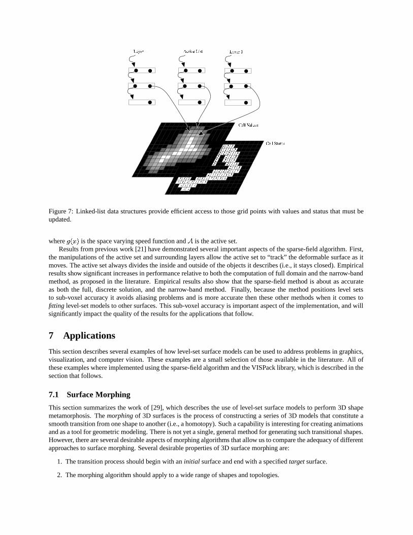
Figure7: Linked-list datastructuresprovide efficient accessto thosegrid points with valuesandstatusthatmustbeupdated.
where*µ! # is thespacevarying speedfunctionand ® is theactiveset.
Resultsfrom previouswork [21] have demonstratedseveralimportantaspectsof thesparse-fieldalgorithm. First,themanipulationsof theactive setandsurrounding layersallow theactive setto “track” thedeformablesurfaceasitmoves.Theactivesetalwaysdividestheinsideandoutsideof theobjects it describes(i.e., it staysclosed).Empiricalresultsshow significantincreasesin performancerelative to boththecomputationof full domainandthenarrow-bandmethod, asproposedin the literature. Empirical resultsalsoshow that the sparse-fieldmethod is about asaccurateas both the full, discretesolution, and the narrow-bandmethod. Finally, becausethe method positionslevel setsto sub-voxel accuracy it avoids aliasingproblemsandis moreaccuratethentheseothermethods whenit comestofitting level-setmodelsto othersurfaces. This sub-voxel accuracy is importantaspectof theimplementation,andwillsignificantlyimpactthequalityof theresultsfor theapplicationsthatfollow.
7 Applications
This sectiondescribesseveral examplesof how level-setsurfacemodelscanbeusedto addressproblemsin graphics,visualization, andcomputervision. Theseexamples area small selectionof thoseavailablein the literature. All oftheseexampleswhereimplementedusingthesparse-fieldalgorithm andtheVISPacklibrary, whichis describedin thesectionthatfollows.
7.1 SurfaceMor phing
This sectionsummarizesthework of [29], which describes theuseof level-setsurfacemodelsto perform 3D shapemetamorphosis.Themorphingof 3D surfacesis theprocessof constructing a seriesof 3D models thatconstituteasmoothtransitionfrom oneshapeto another(i.e.,ahomotopy). Suchacapabilityis interestingfor creatinganimationsandasatool for geometricmodeling. Thereis notyetasingle,general method for generatingsuchtransitional shapes.However, thereareseveraldesirable aspectsof morphingalgorithmsthatallow usto comparetheadequacy of differentapproachesto surfacemorphing. Several desirablepropertiesof 3D surfacemorphingare:
1. Thetransitionprocessshould begin with an initial surfaceandendwith aspecifiedtargetsurface.
2. Themorphing algorithm should applyto a wide rangeof shapesandtopologies.

3. Intermediatesurfacesshould undergocontinuous3D transitions(rather thancontinuityonly in theimagespace).
4. A 3D morphing algorithm shouldincorporateuserinput easilybut shoulddegradegracefully without it.
5. Transitionalshapesshoulddepend only on thesurfacegeometry of thetwo inputshapesanduserinput.
Theserequirementsarenotexhaustive,but they capture many of thepracticalaspectsof 3D morphing.In this sectionwe show how level-setmodelsprovide analgorithmfor 3D morphing which meetsmostof these
criteria andcompare favorably with existing algorithms. Furthermore, this algorithmis a natural extension of themathematicalprinciplesdiscussedin previoussections.Thestrategy is to allow afree-formdeformationof onesurface(calledthe initial surface)usingthesigneddistancetransform of a secondsurface(thetarget surface). This free-formdeformationis combinedwith anunderlying coordinatetransformationthatgiveseithera rough global alignmentofthetwo surfaces,or one-to-onerelationships betweena finite setof landmarks on boththeinitial andtarget surfaces.Thecoordinatetransformationcanbecomputedautomatically or usinguserinput (asin [30]).
Much of the previous 3D morphing work hasfocusedon morphing parametric models [31, 32] andappliestoonly very limited classesof shapesandtopologies. Several authors have described volumetric techniques. Hughes[33] demonstrateshow volumescanprovide topological flexibility in surfacemorphing. Lerioset al. [30] followedup with a volume-basedschemewhich incorporatesuserinput via underlying coordinatetransformations(a knowngeneralizationtheimagewarpingtechnique that is oftenusedin imagemorphing). Neitherof theseapproacheshavedealtwith thedeeperissueof deformingthelevel setsof avolume,but ratherrely onthepropertiesof theembedding.PayneandToga[34] aswell asCohen-Oret al. [35] fix theembedding problemby usinga signeddistancetransformto createvolumesfrom surfaces.However, interpolating distancetransforms canintroduceartifactsthat violate thepreviously statedproperties,andboth of thesemethods usea discretedistancetransformwhich introducesvolumealiasing.
7.1.1 Free-Form Deformations
Thedistancetransform givesthenearestEuclideandistanceto asetof points,curve,or surface. For closedsurfacesin3D, thesigneddistancetransformgivesa positive distancefor pointsinsideandnegative for pointsoutside(onecanalsochoosetheoppositesignconvention).
If two connectedshapesoverlap thentheinitial surfacecanexpand or contractusingthedistancetransform of thetarget. Thesteadystateof suchadeformationprocessis ashapeconsistingof thezerosetof thedistancetransform ofthetarget.Thatis, theinitial objectbecomesthetarget. This is thebasisof theproposed3D morphingalgorithm.
Let ; ! �%# bethesigneddistancetransform of thetargetsurface, ¯ , andlet ° betheinitial surface.Theevolutionprocesswhichtakesa model
�from ° to ¯ is definedbys �s m � p ; ! �%# � (32)
where � ! m #�)-� q and � q+±rÒ �²° . The free-form deformationscan be combined with an underlying coordinatetransformation.Thestrategy is to usea coordinatetransformation(for instancea translationandrotation) to positionthetwo surfacesneareachother. Thesetransformations cancapture grosssimilaritiesin shapeaswell asuserinput.A coordinatetransformationis given by �´³¤�¶µ ! � � 0¥# � (33)
where S ² 0 ² 2 parameterizesa continuousfamily of thesetransformationsthat begins with identity, i.e. � �µ ! � � SQ# . Theevolution equation for a parametricsurfaceiss �s m � p ; ! µ ! � � 2�#�# � (34)
andthecorresponding level-setequationiss¸· ! � ��m #s m ��� = · ! � ��m #>�1; ! µ ! � � 24#�# ( (35)
This processproducesa seriesof transitionshapes(parameterizedby m ). The coordinatetransformationcanbea global rotation,translation, or scaling,or it might be a warpingof the underlying 3D spaceaswasusedby [30].

Figure8: A 3D model of a jet thatwasbuilt usingClockworks,aCSGmodelingsystem.
Incorporating userinput is important for any surfacemorphing technique, becausein many casesfinding the bestsetof transitionsurfacesdependson context. Only userscanapplysemanticconsiderations to the transformationofoneobject to another. However, this underlying coordinatetransformationcan,in general,achieve only somefinitesimilarity betweenthe“warped” initial modelandthetarget, andeventhis mayrequire a greatdealof userinput. Intheevent thata useris not ableor willing to defineevery importantcorrespondencebetweentwo objects,someothermethodmust“fill in” thegaps remaining betweenthe initial andtargetsurface. In [30] they proposealphablendingto achieve thatsmoothtransition—really just a fadingfrom onesurfaceto theother. We areproposingtheuseof thefree-formdeformations,implementedwith level-setmodels,to achieveacontinuoustransitionbetweentheshapesthatresultfrom theunderlyingcoordinatetransformation.Wehavealsoexperimentedwith waysof automatically orientingandscalingobjects,using3D moments, in orderto achieve asignificantcorrespondencebetweentwo objects.
Figure 8 shows a 3D modelof a jet that wasbuilt usingClockworks [36], a CSG modeling system. Lerios etal. [30] demonstratethetransitionof a jet to a dart,which wasaccomplishedusing37 user-definedcorrespondences,roughly a hundreduser-definedparameters. Figure 9 shows theuseof level-setmodelsto constructa setof transitionsurfacesbetweenajet andadart.Thetriangle meshis extractedfrom thevolumeusingthemethodof marching cubes[5]. Theseresultsareobtainedwithoutany userinput. DistancetransformsontheCSGmodelsarecomputednearthelevel surfaceusingananalyticaldescription andextendedinto thevolumeusinga level-setmethod [37].
The application in this sectionshows how level-setmodels moving according to the first-order term given inexpression2 in Table1 can“fit” otherobjectsby moving with a speedthatdependson thesigneddistancetransformof the target object. The applicationin the next sectionrelieson expression5 of Table1, a second-orderflow thatdependson theprincipal curvaturesof thesurfaceitself.
7.2 Filleting and Blending Solid Objects
The construction of blendingsurfacesis an important tool in solid modeling. Geometric solid primitivesandtheirintersections oftenproducesharpcornersor creasesthatareoftennot consistentwith thereal-world objectsthattheyareintendedto represent. Thissectionshowshow blending canbedescribedasadeformationprocess,wheresurfacesmove under a geometric flow thatcanaddor remove materialbasedon local curvature information. The resultis amethodfor solid objectblending that does not depend on any particular model representation.Thusthis methodisnot restrictedto a specificclassof shapesor topologies. Additionally, the resultsareinvariant; they do not dependon arbitrary choicesof coordinatesystemsor bases.Theonly requirementis thattheblendedobjectsmustbeclosedsurfaceswith someknown inside-outsidefunction.
Surfaceblending techniquesaretypically tied very closelyto the choiceof geometric primitives. For instance,

(a) (b)
(c) (d)
(e) (f)
Figure9: The deformationof the jet to a dart usinga level-setmodel moving with a speeddefinedby the signeddistancetransform of thetargetobject.

Middleditch andSears[38] proposea set-theoretic methodfor blending solidswhich relieson low-order algebraicprimitives.A fillet at thejoint of two tori requiresthesolutionof adegree32polynomial. Bloomenthal andShoemake[39] proposea modeling systembasedon convolutions,which relieson a skeletonizedrepresentationof objects. Ingeneral theuseof convolution to achievedeformationson implicit shapesresultsin shapesthatreflectboththeshapeof themodelandtheembedding,
·.
Theblending method proposedin thissectionimplementsaninterativesmoothing schemethatsmoothsonly alongthelevel set;thefinal resultis independent of theembedding. Considerthecaseof fillets. We proposethata fillet canbeconstructedfrom a processof “filling in” materialin placesof high curvature.Thecurvature of a level-setmodelcanbecalculatedfrom theembedding, andthedeformationof the level setis well definedby thecurvature termsinTable1.
Thestrategy is toconstructacurvatureterm, �º¹ , thatconsistsof onlypositivecurvatures.2 Theprincipal curvaturesof the level setsof
·arefunctions of
·andits derivatives. For a specific
·theprincipal curvaturesarefunctionsof
3-space��? ! �%# and �zA ! �%# . For adding materialthejoint betweentwo objects,we consider only thepositive curvaturecomponents,i.e., s»·s m ��� = · � �¼¹ ��� = · � � n? U � = · � � nA � (36)
where� n consistsof only thepositivepartsof � andis definedaszeroelsewhere.Becausetheuseof separatecurvaturetermscancauseover-shooting, theup-windscheme(treating�¸¹ asaspace-varying velocity in thenormaldirection) isusedfor this evolution.
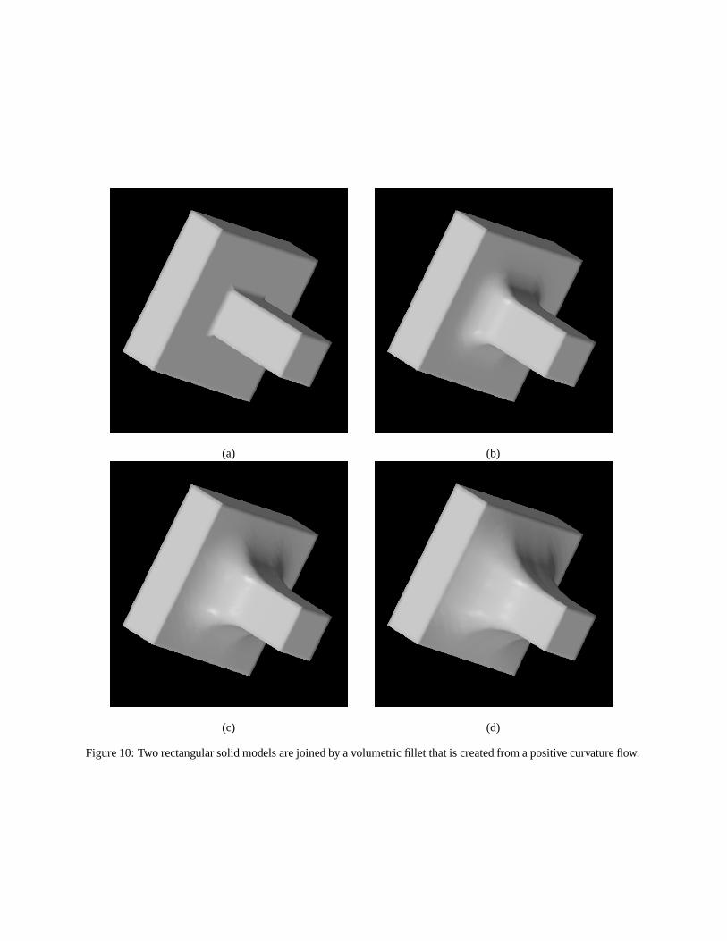
Figure 10shows how thepositive-curvature flow canbeusedto construct fillets. No knowledgeof theunderlyingmodels is necessary. Thefillets grow larger asmoretime passes.Thephysicalextent or positionof thefillet canbecontrolled by eitherspecifying a region of actionor by placinga small blob of deformablematerialin the joint thatrequiresa fillet. Figure11 shows how sucha blending capabilitycanbeuseful in animation. In this casea pair ofsuperquadricsundergo a rigid transformationthatcontrols their relative positions.Level-setmodelswith a positive-curvature flow areusedto createa smoothjoint betweenthesetwo primitives. Notice that the positive curvaturemethoddoesnot suffer from thegrowth or expansionartifactsthatareoftenassociatedwith distance-basedblendingmethods [40].
Thus,asecond-orderflow cancreatesmoothblendsbetweenobjectsin awaythatdoesnotrequirespecificknowl-edgeof theshapesor topologiesof theobject involved. Theapplication in thenext section,3D scenereconstruction,showshow acombinationof first-order andsecond-ordertermsfrom Table1 arecombinedto createtechniquethatfitsmodels to datawhile maintaining certainsmoothnessconstraintsandthereby offsettingtheeffectsof noise.
7.3 3D Reconstructionfr om Multiple RangeMaps
Level-setmodelsareusefulfor problemsrelatedto 3D reconstruction. Previous work haspresented level-setresultsderived from noisy3D datasuchasMRI [19] andultrasound [41]. In [42] we have shown how thereconstructionofobjectsfrom multiple rangemapscanbeformulatedasa problem of finding thesurfacethatoptimizes theposteriorprobability givena setof measurements (noisy range maps)andsomeinformationabout the a-priori probability ofdifferentkindsof surfaces.Thatoptimizationproblemcanbeexpressedasavolumeintegral whichcanbesolvedwithlevel-setmodels. This sectionpresents themathematicalexpressions thatresultfrom thoseformulationsandpresentssomenew results:thereconstructionof entirescenesby fitting level-setmodelsto thedatafrom a scanningLADAR(laserranging anddetection)system.
A rangemapis acollectionof rangemeasurementstakenalongdifferentdirections(linesof sight)but fromasinglepointof view. Rangemapscouldcomefrom any numberof differentsourcesincluding laserscanners,structuredlightdepthsystems,shapefrom stereo,or shapefrom motion. We assumethatsuchrangemapsarenoisyanduncertain.Thegoalis to combine a numberof rangemapsfrom differentpointsof view to createa 3D structure thatreflectsthecollectiveconfidenceanddepthmeasures.
Several examples in theliteraturehave appliedparametric modelsto this task.Turk andLevoy [43], for instance,“zip” togethertriangle meshesin order to construct 3D objectsfrom sequences of rangemapsfrom a laserrangefinder. They perform minor adjustmentsto the surfacepositionin orderaccount for ambiguity in the range maps.Their approachassumesvery little noisein theinput,which is reasonablegiventhehigh quality of their range maps.ChenandMedioni [44] usea parametric (triangle mesh)modelwhich expandsinsidea sequence of range maps.
2Thesignof curvatureis defined by thedirection of thenormals—in this work normalspoint into thevolumeenclosedby theobject.
(a) (b)
(c) (d)
Figure10: Two rectangularsolidmodelsarejoinedby avolumetric fillet thatis createdfrom apositivecurvatureflow.

(a) (b)
(c) (d)
(e) (f)
Figure11: A shortanimationis createdby specifying therelativemotion betweentwo superquadriccomponentsof anobject.A positive-curvature flow (applied frameby frameto thejoint betweenthetwo 3D models)createsa smooth,flexible object.

CurlessandLevoy [45] describea volume-basedtechnique for combining rangedata. They usethesigneddistancetransform to encodevolumeelementswith datathat representthe averages(with someallowancefor outliers) ofmultiple measurements.Surfacesof objectsarethe level setsof volumes. Relatedapproachesaregivenin [46, 47].Bajaj et. al. [48] usea Delaunaytriangulation to imposea topology on a setof unordered3D points andthenfittrivariateBernstein-Bezierpatches—i.e.a higher-order implicit model—tothe data. Muraki [2] usesimplicit orblobby models to reconstruct objectsfrom range data.Theindividual blobsarespherically symmetric3D potentialsthatarecombined linearly so that they blendtogether. Theresultingmodels,with approximately400primitives arequitecoarse.
This work differs from previous work in two ways. First, ratherthanheuristics,our reconstructionstrategy isbasedon a strategy that solvesfor the optimal surfaceestimate.This optimal estimateincludesinformationaboutone’s expectationsof the likelihood of differentsurfaces. The result is not a closed-form solution, but an iterativeprocessthatseeksto fit a level-setmodelto thedatawhile enforcing a kind of smoothnesson thedata.
7.3.1 Objective function for multiple rangemaps
Theevolution equationfor theestimationof optimal surfacesis shown in [42] to consistof two parts:s �s m ��F7{ ! �%# p U¾½ ! �¿# ( (37)
Thisfirst part, F7{ ! �%# p , is thedataterm,which is a movementwith variablespeed(asin expression2 from Table1)that is thecumulative effect from all of the individual rangemaps.Thesecondpart is theprior, which describesthelikelihood of thesurfaceindependentof thedata.Thedatatermis
{ ! �%#��/¨ � ¿ � � � ! �%#¥; � � � ! �%#ÁÀ Ä ; � . � ! �%# Æà� � � ! �%# � (38)
where ; � is thesigneddistancealongtheline of sightfrom a range measurement in rangemap � associatedpassingthrough � . Thefunction À �P� ~�� �
is a windowing function that limits thepenaltyof any onerange measurement,and ¿ ! � # is a confidence function, which is inversely proportional to the level of noisein the rangemeasurementassociatedwith thesameline of sight. Theterm
 ! � # is anintegrationconstant thattakesinto account thecurvilinearcoordinatesystemof therange scanner.
Thus, a set of rangemapscreatesa scalarfunction of 3D, which describesthe movementof a surfacemodelas it seeksthe optimal surfaceposition. In the absenceof a prior, ½ � S , the zerosetof this function is the finalposition(steadystate)of thatevolving surface.Thus, in theabsenceof a prior, onecouldsample
*µ! �%# andobtainanapproximationto theoptimal surfaceestimate.Thisstrategy resultsin analgorithm thatis verymuchlike thatof [45].
There areseveralreasons for goingto aniterativeschemefor finding optimal solutions.First is theuseof a prior.In surfacereconstruction,evena very low level of noisecandegradethequality of therenderedsurfacesin thefinalresult,andin suchcasesbetterreconstructionscanbeobtained by introducingaprior. Secondis aliasing.Discretizing*µ! �%# andfinding thezerocrossingswill causealiasingin thoseplaceswherethe transitionfrom positive to negativeis particularly steep.A deformablemodelcanplacethesurfacemuchmoreprecisely. Thethird reasonfor going toan iterative schemeis that despitethe windowing function À ! �%# thereis interferencebetweendifferent range mapsat placesof high curvature. This problem is addressedby introducinga nonlinearity which is solved in an iterativeschemegivenby equation 37. In thework describedin [21], thesolutionof the linearproblem, thezerosetof
*�! �%# ,servesastheinitial estimatefor thenonlinear, iterative optimization strategy thatresultsfrom theinclusionof a priorandanonlineartermthatcompensatesfor lackof any explicit modelof selfocclusions.
Equation37 includesa prior, which is a likelihood function on surface shape.A reasonable choiceof prior is onethatmodelsobjectswith lesssurfaceareaasmorelikely thanobjectswith moresurfacearea.Alternatively, onecouldsaythatgivena setof surfacesthatarenearthedata,thealgorithm shouldchoosea surfacethathaslessarea.Often,but notalways,thiswill bethesmoothersurface. The ½ ! �¿# thatresultsfromthisprior is themeancurvature.Thereforetheevolution of thesurface,usingthelevel-setformulation, thatseeksto maximizetheposteriorprobability (given asetof range mapsandaprior thatpenalizessurfacearea)iss¸· ! � ��m #s m ��� = · ! ��#N��¨ � Ä ; � � � ! �%#ÅÀ Ä ; � . � ! �%# Æ 6  � � � ! �%# ¿ � � � ! �%# � = · � < � � � ! �%# � n= · � < � � � ! �%#ÇÆ U¾È T � (39)

(a) (b)
Figure12: Rangemaps:Synthetic range data2006 200 pixelswith 20%Gaussianwhite noiseof a torusend(a) andside(b).
(a) (b) (c)
Figure13: (a) An analytically-definedmodel of a torus. (b) An initial model (80 6 80 6 40 voxels) is constructedbycombining six pointsof view of a torusandsolvingfor
*�! �%#$�uS . (c) Themodel, which is attractedto therange databut subjectto internalforces,evolvesandsettlesinto a smoother steadystate.
where< � � � ! �%# is theline of sightfrom a range finderto a 3D point, � , È is a freeparameterthatcontrols thelevel ofsmoothing in themodel, and
Tis theexpressionfor themeancurvature given in equation 6.
Figure 12 shows a pair of simulatedrange mapsconstructed from an analytical descriptionof a torus. These2006 200 pixel range mapsarecorruptedwith additive Gaussiannoisethat hasa standarddeviation of 20% (asafunction of thesmallerof thetwo radii). Six syntheticnoise-corrupted viewpointsof a torusarecombinedto createalevel-setreconstructionof a torus. Figure13(a)showstheinitial model(80 6 80 6 40 voxels)usedfor fitting a level-setmodels to therangedata.Figure13(b) shows theresultof the level-setmodelsthatuses13(a) asan initial stateandhasa valueof È equalto S (ÊÉ . Theresultis a reasonable reconstruction of thenoiselessmodel (Figure13(c)) whichcombinesthesix points of view andthesmoothing function.
Figure 14(a) shows a rangemaptakenwith thePerceptron modelP5000, an infra-red, time-of-flight laserrangefinderwith a pan-tilt mechanism.Figure14(b) shows theamplitudesassociatedwith thereturnsignal(an intensity),and14(c)shows a surfaceplot of the range mapto demonstratethe degreeof noise(additive andoutliers). Figure14(d) shows the confidencevalues associatedwith thoserangemeasurements.Theseconfidence valuesarederivedfrom empiricaldataabout the level of noisein the range finder (which depends on the returnamplitude), andsomeanalysis,from first principles,about theeffectsof uncertaintyin the3D positionsof thescansandthemodel— whichresultsin thelowerconfidenceatedgesasdescribedin [42]. We combinedtwelvesuchviews from different locations

(a) (b)
(c) (d)
Figure14: (a) Oneof twelve range maps(b) The associatedamplitude map(c) A surfaceplot of the range datatoshow thelevel of noise.(d) Theconfidencemeasuresassociatedwith thoserangevalues.

in theroom to generatetheresultsthatfollow.Figure 15(a)shows the initial estimatebasedon the zerocrossingsof
*µ! ��# , and15(b) shows the result of 32iterationswith the prior term andthe correctionfor the surfacenormal direction. The sizeof the volumeis CBSBS+62 É S�6+245BS voxels, andtheresolutionis 1.8cm/voxel. Theseresultsshow theability of thestatistically-basedapproachto overcomethenoisein thescanner, andthey show thatthe inclusionof iterative, model-fitting schemehelpscreatemoreaccurate reconstructions.Theresolution of themodel fallsbelow thatof thescans,becauseit waslimited by therandom-access-memoryavailableonourworkstation. Somesmallfeatures,suchasthearmrestsof thechairs,arelostbecauseof theinaccuraciesin theregistrationof theindividual rangemaps.
8 VISPACK
8.1 Intr oduction
VISPACK is a setof C++, object-orientedlibraries for imageprocessing,volumeprocessing, andlevel-setsurfacemodeling. It consistsof five libraries: Matrix, Image, Volume, Util, and Voxmodel (level-set modeling). Theselibrariescanbeusedseparatelyor togetherwhencreatingapplications.
VISPACK incorporateseightbasicdesignattributes.Theseare
Data Handles/Copyon Write: VISPackis anobject-orientedlibrary, andassuchwe allow theobjects to handlememory management,andrelieve theprogrammer(in mostcases)from having to worry pointers andthecor-responding memory allocation/deallocationproblems. For this we usethe datahandles with a copy on writeprotocol. Copy constructors perform a shallow copy with referencecounting until a nonconst operationon theunderlyingbuffers forcesa deepcopy. Thusdeepcopiesareperformedonly whennecessary, but all memory ismaintainedby theobjectsandobjectsbehave as“variables”ratherthanpointers.
Modified Data Hiding: Accessto datain objects is generally throughaccessmethods,however, pointers to buffersfor fastimplementationsareavailable.
Templates: VISPackutilizesthetemplating constructof C++ virtually throughout. Many of theobjects, includingimages, volumes,lists, andarrays, are intended to support a wide rangeof datatypes. Thus,via templatingprogrammerscandefinethepixels of differentimagesof differenttypes,suchasfloatingpoint, 24-bitcolor, and16-bit greyscale.
Useof Standard File Formats: WhenappropriateVISPackusesstandardfile formats.We chooseformats thatarewell known andhave publicly availablelibrariesthatcanbedistributedwith our libraries. Thematrix libraryusesasimpletext format. TheimagelibraryusesTIFF andFITSfile formats.Becausenostandard formatexistsfor saving volumes of datawe dousea rawfile format.
Operator Overloading: Properuseof operator overloading givesusersa convenient way to execute operationson an object. Whencompined with the copy-on-write convention,operator overloading allows programmersto treatmany heavy-weightobjects(e.g. imagesandvolumes)asvariables. For instance,the following codecomputesnon-maximal edgesin a onafilteredvolume.
Volume<float> dx, dy, dz;Volume<float> vol gauss = vol.gauss(0.5);Volume<float> vol out = (((dx = vol gauss.dx()).power(2)
*vol gauss.dx(2)+ ((dy = vol gauss.dy()).power(2)*vol gauss.dy(2)+ ((dz = vol gauss.dz()).power(2)*vol gauss.dz(2)+ dx*dy*(dx).dy() + dx*dz*(dx).dz())+ dy*dz*(dy).dz()) )).zeroCrossings()
&& ((dx.power(2) + dy.power(2)) > T*T));
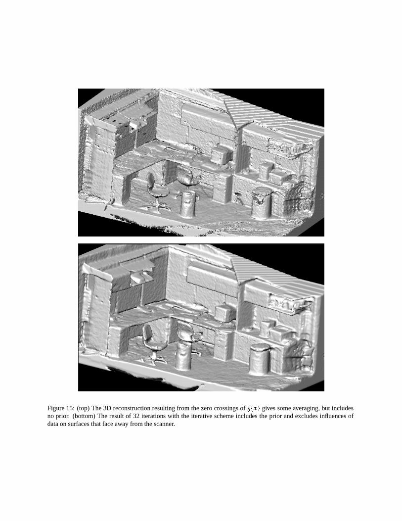
Figure15: (top) The3D reconstructionresultingfrom thezerocrossingsof*µ! ��# gives someaveraging, but includes
no prior. (bottom) Theresultof 32 iterations with the iterative schemeincludestheprior andexcludesinfluencesofdataonsurfacesthatfaceaway from thescanner.
8.2 Level-SetSurface-Modeling Library
TheLevel-SetSurface-Modeling (LSSM)Library is animplementationof thelevel-settechnique[11, 13] specificallyfor deforming surfacemodelsembedded in volumes. The implementationusesthesparse-fieldmethoddescribedin[20]. The library implementsall of thebasicnumerical algorithmsandhandlesall of thedatastructuresrequired toperform LSSM. Thestrategy for usingthis library is to subclasstheobject VoxModel, setsomeparameters, definea setof simplevirtual functions thatcontrol thedeformationprocess,initialize themodel,andthendirect themodelto iteratively deform according to thoseequations. This sectiondescribes the relationshipbetweenthemathematicsof previoussectionsandtheVISPacklibrary. Its alsopresentsanexample of usingVISPacklibarary to do 3D shapemetamorphosisasdescribedin Section7.1.
8.2.1 SurfaceDeformation
The LSSM library allows oneto solve for surfacedeformations,asa function of time, for general level-setsurfacemovementsof theform:s �s m �|0¥y ! � � p ! �%#�# UËÈ { ! � � p ! �%#�# p ! �%# U  p ! �%# U¾ÌÎÍ ! �z? ! �%# �R�QA ! �%#�#�# � (40)
where� is apoint onthesurface.Thisequation is solvedby representingthesurfaceasthe � th level setof animplicitfunction
��! � ��m # �B� � 6 � �nI���� . Thisgivess �s m �f0¥y ! � � = � #�#�� = � UËÈ { ! � � = � #>� = � � U  � = � � U¾ÌÎÍ ! ; � ��� A � # � (41)
where� � and � A � arecollections first andsecondderivativesof�, respectively. Thisequationis solvedonadiscrete
gridusinganup-windschemegradientcalculations,centraldifferencesfor thecurvature,andforward finitedifferencesin time. TheLSSM library usesthesparse-fieldmethoddescribedin Section6.3andin [21].
Thus, theLSSM library offers thefollowing capabilities:
1. Createsaninitial model (with associatedactiveset)from avolume.
2. Calculates� �µ�.�� �R� � and ��m usingvirtual functions(defined bysubclasses)thatdescribey and { , andparameters(valuessetby thesubclass)0 , È ,
Â, and Ì .
3. Performsanupdateon thevaluesof ���.�� �R� � .4. Maintains thelist of active grid pointsandupdatesthe layers around thosepointsin order to maintaina neigh-
borhoodfrom which to calculatesubsequentupdates.
5. Providesaccessto thevolumethatdefines���.c� ��� � andthelinkedlist of activegrid points.
Giventhevolumedefining �¥�.�� �R� � , onecanthenrely on thefunctionality of thevolume library for subsequent process-ing, file I/O, or surfaceextraction.
8.2.2 Structur eand Philosophy of the LSSM Library
Thelibrary is organized(mostlyfor easeof development)into a baseclass,LevelSetModel, anda derivedclass,VoxModel. Thebaseclassdoesall of thebookkeepingassociatedwith the active setandsurrounding layers, thelink lists associatedwith thosesets,andinitializing themodel. Thusit addsandremovesvoxels from theactive set(andsurrounding layers)in responseto anupdateoperation. The baseclassassumesthat thesubclassesknow howto updateindividual voxels. Applications arebuilt by subclassingVoxModel andredefining a small setof virtualfunctionsthatcontrol themovementof themodel.
Thesubclass,VoxModel, performsupdateon thegrid pointsin theactive setof theform givenin Equation16,usingfunctions y and { andparameters0 , È ,
Â, and Ì . It alsocalculatesthemaximum ��m thatensuresstability. Thus
auserwhowishesto performasurfacedeformationusingtheLSSMlibrary, wouldcreatesubclassof VoxModel anddefinetheappropriatevirtual functionsandsettheparametersto achievethedesiredbehavior.

8.2.3 The LevelSetModel Object
TheLevelSetModel containsavolumeof values,avolumeof statusflags,fivelists (oneactivelist, two insidelists,andtwo outsidelists), andthreeparametersthatdetermine theorigin of thecoordinatesystemform which themodelperformsits calculations.
There are two constructors, LevelSetModel() and LevelSetModel( const VISVolume<float>&). Thefirst simply initializesthedatastructure,andthesecondalsosetthevaluesof themodelvolume ( values)to the input. Oncethe valueshave beenset,onecancreatean initial volumefrom thosevaluesby calling con-structLists(), which canalsotake a floating-point argumentthatcontrols thescalingof the input relative to alocaldistancetransform nearthezeroset.
Thelist thatkeeps trackof theactive set,called active list, keepstrackof the locationof thosegrid pointsandasinglefloating-point value,whichstoresthechangein their valuesfrom oneiterationto thenext.
Anotherimportant methodsfor usersof this objectis update(float), whichchangesthegrey-scalevaluesofthegrid for theactivesetaccording to thevalues storedin active list, andupdatesthestatusof elements on theactive list aswell asthevaluesandstatusof nearby layers(2 insideand2 outside).Thefloatingpointargumentis thevalueof ��m from Equation16, andthereturnvalueis themaximum changethatoccurredon theactive set. Finally,the method iterate() calls the virtual methodcalculate change, a virtual function which setsthe valuesof � �µ�.�� �R� � andreturns the maximum valueof ��m for stability, andthencallsupdate. For this objectthe functioncalculate change performssometrivial (i.e.,useless)operation.
8.2.4 The VoxModel Object
TheVoxModel objectis a subclassof LevelSetModel, andit addthreethingsto thebaseclass.
1. calculate change() is redefinedto implement thesurfacedeformationdescribedin Equation41.
2. Thevirtual functionsaredeclared for¦
(calledforce) and { (calledgrow). Thesefunctions aredefinedtoreturn zerofor thisobject.
3. The parameters that control the relative influence of the various terms are read from file by a routineload params.
4. A method rescale(float) is defined, which resamplesthevolumeof grid-point valuesinto a new volumewith differentresolution andredefinesthelists (andtherebythemodel) in this new volume. This method is forperformingcoarse-to-finedeformationprocedures.
8.3 Example: 3D ShapeMetamorphasis
TheMorph objectallowsonetoconstruct asequenceof volumesorsurfacemeshesusingthe3Dshapemetamorphasistechnique described in Section7.1, which was first proposedby Whitaker and Breen[20]. This technique reliesdistancetransformsfor boththesourceandtargetobjects andusesa LSSMsto manipulatetheshapeof thesourcesothatit coincides with thetarget.Thesurfacedeformationthatdescribesthis behavior iss �s m � È { ! µ ! �¥#�# p ! �%# � (42)
where{ ! �%# is simplythedistancetransform (or somemonotonicfunction thereof) of thetarget,and µ is acoordinatetransformationthatalignsthesourceandtargetobjects. Thelevel-setformulationof this iss ��! � ��m #s m � È { ! µ ! ��#�#�� = � � ( (43)
Themorphing processconsistsof severalsteps:
1. Readin distancetransforms(in theform of volumes)for bothsourceandtarget.
2. Initialize theLSSMby fitting it to thezerosetof thesourcedistancetransform.

3. Update theLSSM according to Equation43.
4. Save intermediatevolumes/surfacesat regular intervals.
The remainder of this sectionlists the codeandcommentsfor threefiles, morph.h (which declarestheMorphobject),morph.C (which definesthemethods)andmain.C(which performsall of theI/O andusestheMorph objectto constructa sequence of shapes.
8.4 Mor ph.h
//// morph.h////
#ifndef iris_morph_h#define iris_morph_h
#include "voxmodel/voxmodel.h"#include "matrix/matrix.h"
#define INIT_STATE 0#define MORPH_STATE 1//// This is the morph object. It uses all of the machinery of the base// class to manipulate level sets. It needs to have an initial volume// and a final volume (which would typically be the distance transform,// it might need a 3D transformation, and it needs to redefine the// virtual function "grow", which takes 6 floats as input, the position// followed by the normal vectors (all will calculated and passed into// this method by the base class). It might also have a state, that// indicates whether or not it’s been initialized.//// Functions not defined here should be defined in "morph.C"//class Morph: public VoxModel{
protected:VISVolume<float> _dist_source;VISVolume<float> _dist_target;VISMatrix _transform;
//// This is the function that is used by the base class to manipulate thelevel// set. You can define it to by anything you want. For this object, itwill// return a value from the distance transform of the target.//
virtual float grow(float x, float y, float z,float nx, float ny, float nz);
// There are two states. In the first state, the model is trying to fit// to the input data. In this way the models starts by looking just like
// the input dataint _state;
public:
Morph(const Morph& other){
_dist_target = other._dist_target;_initial = other._initial;_state = MORPH_STATE;_transform = VISVISMatrix(3, 3);_transform.identity();
// initialize();}
Morph(VISVolume<float> init, VISVolume<float> d):VoxModel()
{_dist_target = d;_initial = init;_state = MORPH_STATE;_transform = VISVISMatrix(3, 3);_transform.identity();
// initialize();}
void initialize();
// for this object I assume that the transform is just a matrix.// but it could be anything
void transform(const VISVISMatrix& t){ _transform = t;}
const VISVISMatrix& transform(){ return(_transform);}
void distance(const VISVolume<float> d){ _dist_target = d;}VISVolume<float> distance(){ return(_dist_target);}
};#endif
8.5 Mor ph.C
#include "morph.h"#include "util/geometry.h"#include "util/mathutil.h"
//// this is the virtual function, that is the guts of it all.

//
float Morph::grow(float x, float y, float z,float nx, float ny, float nz)
{
// this says you are in the morph state (things have been initialized)if (_state == MORPH_STATE)
{float xx, yy, zz;VISPoint p(4u);p.at(0) = x;p.at(1) = y;p.at(2) = z;p.at(3) = 1;VISPoint p_tmp;
// this is where you could put some other transform.p_tmp = _transform*p;
xx = p_tmp.x();yy = p_tmp.y();zz = p_tmp.z();
// make sure you are not out of the bounds// of your distance volume.if (_dist_target.checkBounds(xx, yy, zz))
// if not, get the distance (use trilinear interpolation).return(_dist_target.interp(xx, yy, zz));
elsereturn(0.0f);
}else
{// if you are still initializing, then move toward the zero set of// your initial caseif (_initial.checkBounds(x, y, z))
return(_initial.interp(x, y, z));else
return(0.0f);}
}
// this makes the model look like the input.#define INIT_ITERATIONS 5void Morph::initialize(){
_values = _initial;int state_tmp = _state;_state = INIT_STATE;construct_lists(DIFFERENCE_FACTOR);
// these couple of iterations are required to make sure that the zero// sets of the model match the zero sets of the//

for (int i = 0; i < INIT_ITERATIONS; i++){
// limit the dt to 1.0 so that the model settles in to a solutionupdate(::min(calculate_change(), 1.0f));
}_state = state_tmp;
}
8.6 Main.C
#include "vol/volume.h"#include "vol/volumefile.h"#include "image/imagefile.h"#include "morph.h"#include <string.h>
const int V_HEIGHT = (40);const int V_WIDTH = (40);const int V_DEPTH = (40);
#define XY_RADIUS (12) // this matches the 2.5D data generated intorus.C#define T_RADIUS (4) // this matches the 2.5D data generated in torus.C#define S_RADIUS (12) // radius of a sphere
#define B_WIDTH (20.0f)#define B_HEIGHT (60.0f)#define B_DEPTH (20.0f)
#define B_CENTER_X (12.0f)#define B_CENTER_Y (32.0f)#define B_CENTER_Z (12.0f)
float sphere(unsigned x, unsigned y, unsigned z);float torus(unsigned x, unsigned y, unsigned z);float cube(unsigned x, unsigned y, unsigned z);
// This is a program that does the morph. If you give it two// arguments, it reads the initial model and the dist trans for the// final model from the two file names given, otherwise, it makes asphere// and deforms it into a torus
main(int argc, char** argv){
VISVolume<float> vol_source, vol_target;VISVolumeFile vol_file;int i;char fname[80];

vol_source = VISVolume<float>(25,65,25);vol_source.evaluate(cube);
if (argc > 2){
// read in the sourceing modelvol_source = VISVolume<float>(vol_file.read_float(argv[1]));
// read in the dist trans of the final modelvol_target = VISVolume<float>(vol_file.read_float(argv[2]));
}else// make up some volumes
{vol_source = VISVolume<float>(V_WIDTH, V_HEIGHT, V_DEPTH);vol_source.evaluate(sphere);vol_target = VISVolume<float>(V_WIDTH, V_HEIGHT, V_DEPTH);vol_target.evaluate(torus);
}
// create morph objectMorph morph(vol_source, vol_target);// loads in some parameters (for morphing these are all zero but one)// i.e.////////morph.load_parameters("morph_params");morph.initialize();vol_file.write_float(morph.values(), "morph0.flt");
float dt;
// do 150 iterations for your model to get from start to finish// probably don’t need this many iterations
for (i = 0; i < 150; i++){
dt = morph.calculate_change();// limit dt to 0.5 so that model never overshoots goaldt = min(dt, 0.5f);morph.update(dt);
printf("iteration %d dt %f\n", i, dt);
if (((i + 1)%10) == 0){
// save every tenth volumesprintf(fname, "morph_out.%d.dat", i + 1);vol_file.write_float(morph.values(), fname);
}}
// save a surface model (i.e. marching cubes).vol_file.march(0.0f, morph.values(), ‘‘morph_final.iv’’);
printf("done\n");
}
References
[1] J.Blinn, “A generalizationof algebraicsurfacedrawing,” ACM Trans.on Graphics, vol. 1, pp.235–256, March1982.
[2] S.Muraki, “Volumetricshapedescription of rangedatausing“blobby model”,” in SIGGRAPH ’91 Proceedings(T. W. Sederberg, ed.),pp.227–235,July1991.
[3] G. Taubin,“An accuratealgorithm for rasterizingalgebraic curvesandsurfaces,” IEEE ComputerGraphics &Applications, March1994.
[4] D. Breen,S.Mauch,andR. Whitaker, “3d scanconversionof csgmodelsinto distance,closest-point andcolourvolumes,” in VolumeGraphics (M. Chen,A. Kaufman, andR. Yagel,eds.),pp. 135–158, London: Springer,2000.
[5] W. Lorenson andH. Cline, “Marching cubes:A high resolution 3D surfaceconstruction algorithm,” ComputerGraphics, vol. 21,no.4, pp.163–169, 1982.
[6] M. Levoy, “Display of surfacesfrom volume data,” IEEE ComputerGraphics andApplications, vol. 9, no. 3,pp.245–261,1990.
[7] R. A. Drebin,L. Carpenter, andP. Hanrahan, “Volumerendering,” in SIGGRAPH ’88 Proceedings, pp.65–74,August 1988.
[8] J.Sethian,LevelSetMethodsandFastMarching Methods. Cambridge:CambridgeUniversity Press,seconded.,1999.
[9] M. Kass,A. Witkin, andD. Terzopoulos,“Snakes: Active contour models,” International Journal of ComputerVision, vol. 1, pp.321–323, 1987.
[10] D. Terzopoulos andK. Fleischer, “Deformablemodels,” TheVisual Computer, vol. 4, pp.306–331,December1988.
[11] S. OsherandJ. Sethian,“Frontspropagatingwith curvature-dependent speed:Algorithms basedon Hamilton-Jacobiformulations,” Jrnl. of Comp.Phys., vol. 79,pp.12–49,1988.
[12] J. A. Sethian,“A fastmarching level setmethodfor monotonically advancing fronts,” Proc. Nat. Acad.Sci.,vol. 93,no.4, pp.1591–1595, 1996.
[13] J. A. Sethian,Level SetMethods: Evolving Interfaces in Geometry, Fluid Mechanics,ComputerVision, andMaterial Sciences. CambridgeUniversityPress,1996.
[14] S. OsherandR. Fedkiw, “Level setmethods: An overview andsomerecent results,” Tech.Rep.00-08, UCLACenterfor AppliedMathematics,Department of Mathematics,University of California,LosAngeles,2000.
[15] L. AlvarezandJ.-M. Morel, “A morphological approachto multiscaleanalysis:Fromprinciples to equations,”in Geometry-DrivenDiffusionin ComputerVision (B. M. ter HaarRomeny, ed.),pp. 4–21, Kluwer AcademicPublishers,1994.

[16] V. Caselles,R. Kimmel, andG. Sapiro,“Geodesicactivecontours,” in Fifth Int. Conf. onComp.Vision, pp.694–699, IEEE,IEEEComputer SocietyPress,1995.
[17] B. B. Kimia andS. W. Zucker, “Exploring the shapemanifold: the role of conservation laws.,” in Shape inPicture: themathematical descriptionof shapein greylevel images(Y.-L. O, A. Toet,H. Heijmans,D. H. Foster,andP. Meer, eds.),Springer-Verlag, 1992.
[18] R. Malladi, J. A. Sethian,andB. C. Vemuri, “Shapemodeling with front propagation: A level setapproach,”IEEETransactionsonPatternAnalysisandMachineIntelligence, vol. 17,no.2, pp.158–175, 1995.
[19] R. T. WhitakerandD. T. Chen,“Embeddedactivesurfacesfor volume visualization,” in SPIEMedicalImaging1994, (Newport Beach,California), 1994.
[20] R. Whitaker andD. Breen,“Level-setmodels for thedeformationof solid objects,” in TheThird InternationalWorkshoponImplicit Surfaces, pp.19–35, Eurographics,1998.
[21] R. T. Whitaker, “A level-setapproachto 3D reconstruction from range data,” Int. Jrnl. of Comp.Vision, vol. Oc-tober, no.3, pp.203–231, 1998.
[22] R.T. Whitaker, “Algorithmsfor implicit deformablemodels,” in Fifth Intern.Conf. onComp.Vision, IEEE,IEEEComputer SocietyPress,1995.
[23] S. Kichenassamy, A. Kumar, P. Olver, A. Tannenbaum,andA. Yezzi, “Gradient flows andgeometric activecontour models,” in Fifth Int. Conf. onComp.Vision, pp.810–815, IEEE,IEEEComputer SocietyPress,1995.
[24] A. Yezzi,S.Kichenassamy, A. Kumar, P. Olver, andA. Tannenbaum,“A geometricsnakemodel for segmentationof medicalimagery,” IEEETransactionsonMedicalImaging, vol. 16,pp.199–209, April 1997.
[25] L. Lorigo, O. Faugeraus,W. Grimson, R. Keriven, andR. Kikinis, “Segmentationof bonein clinical knee MRIusingtexture-basedgeodesicactivecontours,” in MedicalImageComputingandComputer-AssistedIntervention(MICCAI ’98) (W. Wells,A. Colchester, andS.Delp,eds.),pp.1195–1204,October1998.
[26] S. OsherandJ. Sethian,“Frontspropagatingwith curvature-dependent speed:Algorithms basedon Hamilton-Jacobiformulations,” Jrnl. of Comp.Phys., vol. 79,pp.12–49,1988.
[27] X. XueandR. Whitaker, “Variable-conductance,level-setcurvature for imagedenoising,” in IEEEInternationalConferenceon ImageProcessing, p. To Appear., October 2001.
[28] D. AdalsteinandJ.A. Sethian,“A fastlevel setmethodfor propagating interfaces,” Jrnl. ofComp.Phys., pp.269–277, 1995.
[29] D. BreenandR. Whitaker, “A level-setapproachto 3D shapemetamorphosis,” IEEETransactionsonVisualiza-tion andComputerGraphics, p. To Appear., 2001.
[30] A. Lerios,C. D. Garfinkle,andM. Levoy, “Feature-Basedvolume metamorphosis,” in SIGGRAPH ’95 Confer-enceProceedings(R. Cook,ed.), Annual ConferenceSeries,pp.449–456,Addison Wesley, Aug. 1995.
[31] J.Kent,W. Carlson,andR. Parent,“Shapetransformationfor polyhedralobjects,” in SIGGRAPH ’92 Proceed-ings, pp.47–54, July1992.
[32] J. RossignacandA. Kaul, “AGRELSandBIPs: Metamorphosisasa beziercurve in the spaceof polyhedra,”ComputerGraphics Forum(Eurographics’94 Proceedings), vol. 13,pp.C–179–C–184,September1994.
[33] J. F. Hughes, “Scheduled Fourier volume morphing,” in ComputerGraphics(SIGGRAPH ’92 Proceedings)(E. Catmull,ed.),vol. 26,pp.43–46, July1992.
[34] B. PayneandA. Toga,“Distancefield manipulationof surfacemodels,” IEEEComputerGraphics andApplica-tions, vol. 12,no.1, pp.65–71, 1992.
[35] D. Cohen-Or, D. Levin, andA. Solomivici, “Three-dimensionaldistancefield metamorphosis,” ACM Transac-tionsonGraphics, vol. 17,no.2, pp.116–141, 1998.

[36] P. GettoandD. Breen,“An object-orientedarchitecture for acomputeranimationsystem,” TheVisualComputer,vol. 6, pp.79–92, March1990.
[37] D. Breen,S.Mauch,andR. Whitaker, “3D scanconversionof CSGmodelsinto distancevolumes,” in Proceed-ingsof the1998 SymposiumonVolumeVisualization, pp.7–14, ACM SIGGRAPH,October1998.
[38] A. Middleditch andK. Sears,“Blend surfacesfor settheoreticvolume modelingsystems,” in SIGGRAPH ’85Proceedings, pp.161–170,July1985.
[39] J. Bloomenthal andK. Shoemake, “Convolution surfaces,” in SIGGRAPH’91 Proceedings (T. W. Sederberg,ed.),pp.251–257, July1991.
[40] M. DesbrunandM.-P. Gascuel,“Animating soft substanceswith implicit surfaces,” in SIGGRAPH ’95 Proceed-ings, pp.287–290,August1995.
[41] R. T. Whitaker, “Volumetric deformablemodels: Activeblobs,” in VisualizationIn Biomedical Computing 1994(R. A. Robb,ed.),(Mayo Clinic, Rochester, Minnesota), pp.122–134,SPIE,1994.
[42] R. T. Whitaker, “A level-setapproachto 3D reconstruction from range data,” Int. Jrnl. of Comp.Vision, vol. Oc-tober, no.3, pp.203–231, 1998.
[43] G.Turk andM. Levoy, “Zipperedpolygonmeshesfromrangeimages,” in Proc.of SIGGRAPH’94, pp.311–318,ACM SIGGRAPH,August 1994.
[44] Y. ChenandG. Medioni, “Fitting asurfaceto 3-D pointsusinganinflatingballonmodel,” in Second CAD-BasedVisionWorkshop(A. Kak andK. Ikeuchi, eds.),vol. 13,pp.266–273,IEEE,1994.
[45] B. CurlessandM. Levoy, “A volumetric methodfor building complex models from range images,” in Proc. ofSIGGRAPH ’96, pp.303–312,ACM SIGGRAPH,August 1996.
[46] H. Hoppe, T. DeRose,T. Duchamp, J. McDonald, andW. Stuetzle,“Surfacereconstruction from unorganizedpoints,” ComputerGraphics, vol. 26,no.2, pp.71–78, 1992.
[47] A. Hilton, A. J. Stoddart, J. Illingworth, andT. Windeatt,“Reliablesurfacereconstructionfrom multiple rangeimages,” in Euro. Conf. onComp.Vision, Springer-Verlag, 1996.
[48] C. Bajaj, F. Bernardini, andG. Xu, “Automaticreconstruction of surfacesandscalarfields from 3D scans,” inSIGGRAPH ’95 Proceedings, pp.109–118,August 1995.