issues on content-based image retrieval · issues on content-based image retrieval submitted by sia...
TRANSCRIPT

Issues on Content-Based Image Retrieval
SIA Ka Cheung
A Thesis Submitted in Partial Fulfillment
of the Requirements for the Degree of
Master of Philosophy
in
Department of Computer Science & Engineering
c©The Chinese University of Hong Kong
June 2003
The Chinese University of Hong Kong holds the copyright of this thesis. Any
person(s) intending to use a part or the whole of the materials in this thesis
in a proposed publication must seek copyright release from the Dean of the
Graduate School.

Issues on Content-Based ImageRetrieval
submitted by
SIA Ka Cheung
for the degree of Master of Philosophy
at the Chinese University of Hong Kong
Abstract
This is the abstract....
ii

Acknowledgment
I would like to thank ...
iii

Contents
Abstract ii
Acknowledgement iii
1 Introduction 1
1.1 Problem Statement . . . . . . . . . . . . . . . . . . . . . . . . . 1
1.2 Contribution . . . . . . . . . . . . . . . . . . . . . . . . . . . . . 2
1.3 Thesis Organization . . . . . . . . . . . . . . . . . . . . . . . . . 2
2 Background 3
2.1 Content-Based Image Retrieval . . . . . . . . . . . . . . . . . . 3
2.1.1 Feature Extraction . . . . . . . . . . . . . . . . . . . . . 4
2.1.2 Indexing and Retrieval . . . . . . . . . . . . . . . . . . . 4
2.2 Relevance Feedback . . . . . . . . . . . . . . . . . . . . . . . . . 6
2.2.1 Weight Updating . . . . . . . . . . . . . . . . . . . . . . 7
2.2.2 Bayesian Formulation . . . . . . . . . . . . . . . . . . . . 9
2.2.3 Statistical Approaches . . . . . . . . . . . . . . . . . . . 10
2.2.4 Inter-query Feedback . . . . . . . . . . . . . . . . . . . . 10
2.3 Peer-to-Peer Information Retrieval . . . . . . . . . . . . . . . . 12
2.3.1 Distributed Hash Table Techniques . . . . . . . . . . . . 13
2.3.2 Routing Indices and Shortcuts . . . . . . . . . . . . . . . 15
2.3.3 Content-Based Retrieval in P2P Systems . . . . . . . . . 15
iv

3 Parameter Estimation Based Relevance Feedback 17
3.1 Parameter Estimation of Target Distribution . . . . . . . . . . . 17
3.1.1 Model . . . . . . . . . . . . . . . . . . . . . . . . . . . . 19
3.1.2 Relevance Feedback . . . . . . . . . . . . . . . . . . . . . 19
3.1.3 Maximum Entropy Display . . . . . . . . . . . . . . . . . 21
3.2 Self-Organizing Map Based Inter-Query Feedback . . . . . . . . 23
3.2.1 Motivation . . . . . . . . . . . . . . . . . . . . . . . . . . 23
3.2.2 Initialization and Replication of SOM . . . . . . . . . . . 25
3.2.3 SOM Training for Inter-query Feedback . . . . . . . . . . 26
3.2.4 Target Estimation and Display Set Selection for Intra-
query Feedback . . . . . . . . . . . . . . . . . . . . . . . 28
3.3 Experiment . . . . . . . . . . . . . . . . . . . . . . . . . . . . . 30
3.3.1 Study of Parameter Estimation Method Using Synthetic
Data . . . . . . . . . . . . . . . . . . . . . . . . . . . . . 30
3.3.2 Performance Study in Intra- and Inter- Query Feedback . 35
3.4 Conclusion . . . . . . . . . . . . . . . . . . . . . . . . . . . . . . 37
4 DIStributed COntent-based Visual Information Retrieval 39
4.1 Introduction . . . . . . . . . . . . . . . . . . . . . . . . . . . . . 39
4.2 Peer Clustering . . . . . . . . . . . . . . . . . . . . . . . . . . . 39
4.2.1 Basic Version . . . . . . . . . . . . . . . . . . . . . . . . 40
4.2.2 Single Cluster Version . . . . . . . . . . . . . . . . . . . 42
4.2.3 Multiple Clusters Version . . . . . . . . . . . . . . . . . 46
4.3 Firework Query Model . . . . . . . . . . . . . . . . . . . . . . . 47
4.4 Implementation and System Architecture . . . . . . . . . . . . . 51
4.4.1 Gnutella Message Modification . . . . . . . . . . . . . . 52
4.4.2 Architecture of DISCOVIR . . . . . . . . . . . . . . . . . 53
4.4.3 Flow of Operations . . . . . . . . . . . . . . . . . . . . . 55
4.5 Experiment . . . . . . . . . . . . . . . . . . . . . . . . . . . . . 57
v

4.5.1 Simulation Model of the Peer-to-Peer Network . . . . . . 57
4.5.2 Number of Peers . . . . . . . . . . . . . . . . . . . . . . 59
4.5.3 TTL of Query Message . . . . . . . . . . . . . . . . . . . 62
5 Future Works and Conclusion 64
A Efficient Discovery of Signature Value 65
Bibliography 66
vi

List of Tables
3.1 Parameters of the synthetic data . . . . . . . . . . . . . . . . . 32
3.2 Four dimensional test case data . . . . . . . . . . . . . . . . . . 32
3.3 Six dimensional test case data . . . . . . . . . . . . . . . . . . . 32
3.4 Eight dimensional test case data . . . . . . . . . . . . . . . . . . 33
3.5 Parameters Used in Inter-Query Feedback Experiment . . . . . 36
4.1 Definition of Terms . . . . . . . . . . . . . . . . . . . . . . . . . 43
4.2 Distance Between Signature Values of Peers . . . . . . . . . . . 46
4.3 Characteristics of Each P2P Network Model . . . . . . . . . . . 57
4.4 Experiment Parameters for Scalability Experiment . . . . . . . . 60
4.5 Experiment parameters . . . . . . . . . . . . . . . . . . . . . . . 63
vii

List of Figures
2.1 Feature extraction of Average RGB value. . . . . . . . . . . . . 5
2.2 R-tree indexing structure:(a)2-dimensional data points and bound-
ing rectangles, (b)indexing structure. . . . . . . . . . . . . . . . 5
2.3 Relevance feedback architecture . . . . . . . . . . . . . . . . . . 7
2.4 Feature organization in Rui’s method . . . . . . . . . . . . . . . 8
2.5 LSI model of inter-query feedback . . . . . . . . . . . . . . . . . 11
2.6 Illustration of information retrieval in a P2P network. . . . . . . 13
2.7 Illustration of indices management in CAN . . . . . . . . . . . . 14
2.8 Creation and propagation of routing index . . . . . . . . . . . . 16
3.1 Fitting µ and σ for data points selected to display . . . . . . . . 22
3.2 The expectation function to be maximized . . . . . . . . . . . . 22
3.3 Inter-query feedback illustration . . . . . . . . . . . . . . . . . . 24
3.4 Gaussian Neighborhood Function on a SOM Grid . . . . . . . . 28
3.5 Retrieval process using modified SOM M ′ . . . . . . . . . . . . 30
3.6 RMS of estimated mean and standard deviation along each feed-
back iteration . . . . . . . . . . . . . . . . . . . . . . . . . . . . 33
3.7 Number of feedback given along each feedback iteration . . . . . 33
3.8 Precision-Recall Graph of test case in 4-D data - 1 . . . . . . . . 34
3.9 Precision-Recall Graph of test case in 4-D data - 2 . . . . . . . . 34
3.10 Precision-Recall Graph of test case in 6-D data - 1 . . . . . . . . 35
3.11 Precision-Recall Graph of test case in 6-D data - 2 . . . . . . . . 35
viii

3.12 Precision-Recall Graph Showing Performance in Real Data . . . 37
4.1 Illustration of two types of connections in DISCOVIR. . . . . . 40
4.2 Peer Clustering - Basic Version . . . . . . . . . . . . . . . . . . 41
4.3 Peer Clustering - Single Cluster Version . . . . . . . . . . . . . . 46
4.4 Multiple Clusters Exist in a Peer. . . . . . . . . . . . . . . . . . 48
4.5 Illustration of firework query. . . . . . . . . . . . . . . . . . . . 49
4.6 Screen-shot of DISCOVIR. . . . . . . . . . . . . . . . . . . . . . 52
4.7 ImageQuery Message Format . . . . . . . . . . . . . . . . . . . 53
4.8 ImageQueryHit Message Format . . . . . . . . . . . . . . . . . . 53
4.9 Architecture of DISCOVIR. . . . . . . . . . . . . . . . . . . . . 54
4.10 Power law distribution simulation model. . . . . . . . . . . . . . 58
4.11 Recall against Number of Peers . . . . . . . . . . . . . . . . . . 60
4.12 Query scope against Number of Peers . . . . . . . . . . . . . . . 60
4.13 Query Efficiency against Number of Peers . . . . . . . . . . . . 61
4.14 Generated network traffic against Number of Peers . . . . . . . 62
4.15 Minimum reply path length against Number of Peers . . . . . . 62
4.16 Query Efficiency against TTL value of query packet . . . . . . . 63
ix

Chapter 1
Introduction
“A picture worths thousands words”. What does this idiom tell us? Obviously,
image play a much more more important role than text. The information
contained in an image even can’t be described by words. However, the search
and organization of image databases is often of less importance/attention than
text databases. Plainly, there must be difficulties lie ahead for us to solve.
1.1 Problem Statement
Content-Based Image Retrieval (CBIR) was proposed for nearly ten years,
yet, there are still many open problems left unsolved. According to some re-
searchers [36, 31], the learning of image similarity, the interaction with users,
the need for databases, the problem of evaluation, the semantic gap with im-
age features, and the understanding of images are keys to improve CBIR. In
our research, we target on the first 3 areas. Relevance Feedback (RF) [32, 2]
is a commonly used architecture for refining queries in a search engine. We
aim to devise better methods to interact with users in order to learn the
similarity of images form their feedback. For the database support of CBIR,
Peer-to-Peer(P2P) systems are recently evolved paradigms for achieving higher
1

Chapter 1 Introduction 2
throughput of both data storage and computation power. We forsee the po-
tential for P2P systems in supporting CBIR and demonstrate a working imple-
menation and novel strategy for efficient CBIR over distributed environment.
1.2 Contribution
Adding self-citation is enough?
1.3 Thesis Organization
In this thesis, we review the background on relevance feedback techniques and
P2P systems in Chapter 2. In Chapter 3, we propose and evaluate a parameter
estimation method and a Self-Organizing Map [17] approach in the relevance
feedback architecutre. In Chapter 4, we describe an implementation of CBIR
system in a distributed environment, together with a novel Firework Query
Model to reduce network traffic and improve retrieval performance. Lastly, we
discuss about possible future works and give concluding remarks in Chapter 5.

Chapter 2
Background
Information Retrieval is the exploration or search of a database or the
Internet in order to help people access information in a precise and efficient
manner.
2.1 Content-Based Image Retrieval
As an idiom said “An Image worth thousands words”, even a small image can
convey numerous information. It seems that searching images is much more
difficult than searching text. In early image retrieval system, it requires hu-
man annotation and classification on the image collection, the query is thus
performed using text-based retrieval method. However, there are two limita-
tions for such implementation, Human Intervention1 and Non-Standard
Description2. As a consequence, with the rapid growth in the volume of
digit images, searching and browsing in a large collection of unannotated im-
ages is gaining importance. Content-Based Image Retrieval (CBIR) Systems
are proposed to pass this tedious task to computer. Since early 1990’s, many
systems have been proposed and developed, some of them are QBIC [11],
WebSEEK [37], SIMPLIcity [42], MARS [21], Photobook [27], WALRUS [24]
1The process of annotating images is potentially error prone and tedious.2Different annotators may have different perception on the same image and use different
words to describe it.
3

Chapter 2 Background 4
and other systems for domain specific applications [18, 16]. In CBIR systems,
low-level feature vectors, like texture, color and shape, are first extracted and
indexed to represent images during the retrieval process. In the following two
sections, we will address on two technical backgrounds of CBIR: Feature Ex-
traction, and Indexing & Retrieval.
2.1.1 Feature Extraction
In order to search images based on their contents, a CBIR system must obtain
the content-based feature of its image collection, this process is known as
feature extraction. When an image is added to the collection, several features,
such as color, texture and shape3, are extracted and transformed into feature
vector. Here is the mathematical model of feature extraction:
f : I × θ → Rd (2.1)
where f represents a specific feature extraction method, I is the image
under operation, θ is a set of parameters for feature extraction f , Rd is a real
value d dimension vector as the result of feature extraction. Fig. 2.1 shows the
Average RGB values of an images collection are extracted and represented as
3-dimensional data points.
2.1.2 Indexing and Retrieval
After the feature vectors of images are extracted, they are used to represent the
images during the retrieval process. Unlike text indexing and retrieval problem,
which can be handled by B-tree or inverted file4, there are techniques developed
3Specially, some feature likes Color Histogram, Color Moment, Color Coherence Vector,Tamura, Gabor Wavelet, Fourier Descriptor.
4Inverted file is a data structure commonly used to locate files/websites that containsthe query term in a search engine.

Chapter 2 Background 5
Figure 2.1: Feature extraction of Average RGB value.
to index and retrieve these multi-dimensional points, the most common one is
R-tree as shown in Fig. reffig:rtree.
In most of the CBIR systems, they assume a short distance in the low-
level feature vector space to be the definition of similar images. Under this
assumption, nearest neighbour search is used to locate a set of similar images
in respond to a query.
Figure 2.2: R-tree indexing structure:(a)2-dimensional data points and bound-ing rectangles, (b)indexing structure.

Chapter 2 Background 6
2.2 Relevance Feedback
As described in section 2.1, previous systems are based on the one-shot ap-
proach, in which images with the shortest distance to the query image (in the
form of feature vector) are retrieved and presented to the user. Plainly, this
model is not adaptive to different users; as one might pay more attention to
color of images rather than texture. To adapt to different users’ preference,
relevance feedback architecture is proposed. The goal of relevance feedback is
to learn user’s preference from their interaction, and it is a powerful technique
to improve the retrieval result in CBIR. Under this framework, a set of images
is presented to the user according to the query. The user marks those images
as either relevant or non-relevant and then feeds back this into the system.
Based on this feedback, the system estimates user’s preference through this
learning process. Fig. 2.3 shows a typical relevance feedback process.
Most of the current relevance feedback systems are based on the intra-query
approach. In this approach, the system refine the query by using feedback in-
formation that the user provided. This learning process starts from ground up
for each query. For example, PicHunter [7] presented a Bayesian framework
to direct a search with relevance feedback information. Each image in the
database is associated with a probability being the target image of a user’s
query. The Bayes’s rule is used to update the probability according to user’s
feedback information in every iteration. Rui et al. [32] proposed a weight
updating approach to capture user’s preference on different feature represen-
tations of images. The weight of each feature, its representation and each
dimension is updated by their discriminative power between the set of rele-
vant and non-relevant images in the current query. The similarity measure of
images is thus based on their weighted distance in the feature space. The
intra-query approach uses the feedback information to estimate user’s target
distribution, but it often fails when the underlying distribution is not clustered

Chapter 2 Background 7
Figure 2.3: Relevance feedback architecture
in the low-level feature space. This is due to the feedback information given
by a single query is limited and unable to provide enough statistical informa-
tion about the distribution [43]. In the following sections, we will review the
method proposed by Rui et al. [32], Cox et al. [7] and other researchers.
2.2.1 Weight Updating
In [32], objects in image database are modelled as
O = O(D,F,R), (2.2)
where D is the raw image data, F = {fi} is a set of low level visual features,
such as color, texture, and shape, and R = {rij} is the set of representations
for fi, which is defined as
rij = [rij1, ..., rijk, ..., rijK]. (2.3)
Moreover, the feature vector is organized in a hierarchical manner. The
overall similarity of two images Oa and Ob is defined as
S(Oa, Ob) =∑
i
WiS(f ai , fbi ), (2.4)

Chapter 2 Background 8
Figure 2.4: Feature organization in Rui’s method
S(f ai , fbi ) =
∑
j
WijS(raij, rbij), (2.5)
S(raij, rbij) = m(raij, r
bij,Wijk), (2.6)
where m is the distance measure function, while Wi, Wij and Wijk are the
weights associated with each features, its representation and each dimension
respectively. For each feedback, they will follow the two procedures described
below to update the weight in order to capture user’s interest in different
features. Fig. 2.4 shows the organization of features, representations and di-
menions in this appraoch.
Interweight Updating Procedure
Suppose RT is the set of most similar images according to the overall similarity
function Eq. 2.4, for each feature representation ij, the system retrieves a set
of similar images, RT ij, according to that particular feature representation.
The weight, Wij, is updated according to
Wij =
Wij +R, RT ijl ∈ RT and l = 1, ..., N,
Wij, otherwise

Chapter 2 Background 9
where N is the number of most similar images and R is the degree of relevance
indicated by the user.
Intraweight Updating Procedure
For the set of relevant images indicated by user’s feedback, the system com-
putes the standard deviation, σijk, in each dimension, and the weight for each
dimension is updated as Eq. (2.7). We can see that if σijk is large, then the
dimension is not ideal for discriminating relevant and irrelevant images, so its
weight is updated as follows,
Wijk =1
σijk. (2.7)
2.2.2 Bayesian Formulation
In [7], each image is associated with a probability of being the user’s target.
The retrieval process consists of two steps. In each pass, the system selects a
set of images and presents to user. Through the feedback, the system updates
the likelihood measure to the query of each image accordingly. The probability
is updated using the Bayes’ rule as follows,
P (T = Ti|Ht) =P (At|T = Ti, Dt, St−1)P (T = Ti|Ht−1)∑nj=1 P (At|Tj, Dt, St−1)P (Tj|Ht−1)
. (2.8)
The meaning of Eq. (2.8) is that the probability of Ti being the target image
at iteration t is equal to product of the probability of Ti being the target at
iteration t − 1 and the probability of user give such feedback at iteration t
provided that Ti is the target, over the summation of probability of other
images.
Moreover, as each image is associated with a probability of being the target,
[7] proposed a maximum entropy display strategy to select image presenting
to user. As a result, the system is expected to get most information gain from

Chapter 2 Background 10
user’s feedback. Besides, [16] also details the procedure to apply this strategy.
This method inspires the display model of our proposal.
2.2.3 Statistical Approaches
Nigam et. al. [26] and Wu et. al. [43] also used the EM algorithm to classify doc-
uments and images respectively. Expectation Maximization (EM) algorithm
was first proposed in 1977 [10] . It was used to solve the maximum-likelihood
from incomplete data. Given a mixture of Gaussians, the EM algorithm esti-
mates the parameter of each mixture, say, mean and variance. Our proposed
approach is based on EM algorithm to estimate the parameter of user’s target
distribution which will be detailed in Chapter 3. Their EM approaches utilize
the information contained in unlabeled data5 to help estimating user’s target
distribution more efficiently and accurately. More recently, Tian et. al. [41]
model this as classification problme and tackle it by Support Vector Machine
(SVM). By treating the marked relevant and non-relevant images (their corre-
sponding feature vector) as support vector, SVM is able to delineate a region
containing relevant images with minimized risk of incorrect classification. All
these newly suggested methods tends to model the feedback process as a learn-
ing process and apply algorithms in computer learning to help.
2.2.4 Inter-query Feedback
Recent research propose the use of inter-query information to further improve
retrieval result [15] [14]. The relevance feedback not only provids information
about user’s target distribution and preference, but also a similarity measure of
images under human perception. In this approach, feedback information from
5Unlabeled data means those images not marked by the user as either relevant or non-relevant

Chapter 2 Background 11
Figure 2.5: LSI model of inter-query feedback
individual users are accumulated to train the system to determine which im-
ages are of the same semantic meaning. Heisterkamp [15] and He et al. [14] ap-
plied inter-query information and latent semantic indexing (LSI) [9] to CBIR.
LSI is a classical document retrieval algorithm. It analyzes the correlation of
documents and terms in the database. In this approach, previous feedback
information are stored in the system to build the latent semantic index. Each
query result is considered as a document and each image in the database is
consider as a term, thus the correlation of image and different semantic mean-
ing is revealed. However, these methods can only retrieve images which have
been marked at least once as relevant in the history of previous of query. Thus,
large number of query results is required in order to make sure all images can
be retrieved. Moreover, various inter-query approachs do not concern about
the subjectivity of different users, and the same initial query point always pro-
vide the same query result. Fig. 2.5 illustrate how a system treat images as
terms and successive feedback information as documents ans use LSI method
to retrieve similar images.

Chapter 2 Background 12
2.3 Peer-to-Peer Information Retrieval
Peep-to-Peer (P2P) Network is a recently evolved paradigm for distributed
computing. With the emerging P2P networks or their variants such as Gnutella [13],
Napster [23] and Freenet [12], and their implementations, such as LimeWire [20],
etc. They offer the following advantages:
1. Distributed Resource–The storage, information and computational
cost can be distributed among the peers, allowing many individual com-
puters to achieve a higher throughput [34].
2. Increased Reliability–The P2P network increases reliability by elim-
inating reliance on centralized coordinators that are potential critical
points of failure [6].
3. Comprehensiveness of Information–The P2P network has the po-
tential to reach every computers on the Internet, while even the most
comprehensive search engine can only cover one-third of the indexable6
web-site available as stated in some statistics. [19]
Figure 2.7 shows an classical example of a P2P network7. In the example,
different files are shared by different peers. When a peer initiates a search for
a file, it broadcasts a query request to all its connecting peers. Its peers then
propagate the request to their own peers and this process continues. Unlike
the client-server architecture of the web, the P2P network aims at allowing
individual computer, which joins and leaves the network frequently, to share
information directly with each other without the help of dedicated servers.
Each peer acts as a server and as a client simultaneously. In these networks, a
peer can become a member of the network by establishing a connection with
6Indexable here means not including the non-indexable web-site, which is many timesthe indexable one as stated in some statistics [4]
7It is in fact the Gnutella model

Chapter 2 Background 13
one or more peers in the current network. Messages are sent over multiple hops
from one peer to another while each peer responds to queries for information it
shares locally. Plainly, this model is wasteful because peers are forced to handle
irrelevant query messages. This type of search is called a Breadth-First-Search
(BFS). As shown in this example, the data location process is a key problem
in P2P information retrieval. When a peer issues a query request, the P2P
system must be able to locate the required data in an efficient manner. Many
methods are proposed to solve this problem. They can be divided into two
categories and we are going to introduce them in the following two sections.
Figure 2.6: Illustration of information retrieval in a P2P network.
2.3.1 Distributed Hash Table Techniques
To address the data location problem, Chord [39], CAN [28], Pastry [30] and
Tapestry [45] tackle it by distributing the index storage into different peers,
thus sharing the workload of a centralized index server. The distributed infras-
tructure uses Distributed Hash Table (DHT) technique to map the filename
shared by a peer to a key, and each peer is responsible for storing a certain

Chapter 2 Background 14
range of (Key, Value)8 pairs. When a peer looks for a file, it hashes the file-
name to a key and asks the peers responsible for this key for the actual storage
location of that file. Chord models the key as an m-bits identifier and arranges
the peers into a logical ring topology to determine which peer is responsible
for storing which pair (Key, Value). CAN models the key as point on a d-
dimension Cartesian coordinate space, while each peer is responsible for (Key,
Value) pairs inside its specific region. Fig. ?? illustates how CAN distributes
indices into different peers. Such systems take a balance between the central-
ized index and totally decentralized index approaches. They speed up and
reduce message passing for the process of key lookup (data location). Some
extensions of DHTs to perform content-based retrieval and textual similarity
matches instead of filename match are proposed in [40]. Although DHTs are
elegant and scalable, their performance under the dynamic conditions for P2P
systems in unknown[29]. Moreover, such kind of schemes rely on the trustwor-
thiness of peers participating in the network. The malicious peers are supposed
to be responsible for answering queries but the problem become serious when
they deny to respond under the condition of no duplicate index storage in
other peers.
Distributed Hash Table (DHT) fuction
Peers in the network, storing the (key,value)
pairs of shared files
Files shared by peers
Hash value of filename
Figure 2.7: Illustration of indices management in CAN
8Key is the hashed value of filename and Value is the filename and location
Chapter 2 Background 15
2.3.2 Routing Indices and Shortcuts
As DHTs mandate a specific network structure and queries are based on doc-
ument identifiers, researchers proposed methods that operate under the preva-
lent P2P environment, like Gnutella, and queries are based on content of doc-
uments. Crepso [8] proposed a routing indices approach for retrieving text
documents in P2P systems. Under this scheme, each peer maintains a routing
index to assist in forwarding queries to peers that contain more documents
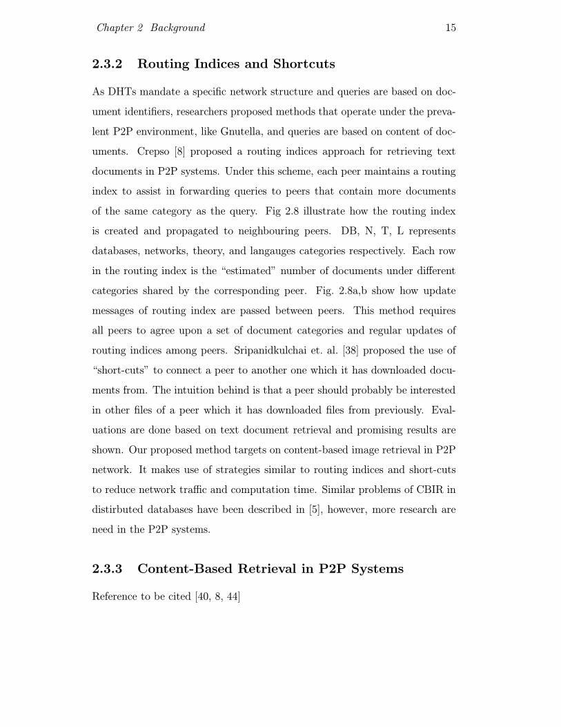
of the same category as the query. Fig 2.8 illustrate how the routing index
is created and propagated to neighbouring peers. DB, N, T, L represents
databases, networks, theory, and langauges categories respectively. Each row
in the routing index is the “estimated” number of documents under different
categories shared by the corresponding peer. Fig. 2.8a,b show how update
messages of routing index are passed between peers. This method requires
all peers to agree upon a set of document categories and regular updates of
routing indices among peers. Sripanidkulchai et. al. [38] proposed the use of
“short-cuts” to connect a peer to another one which it has downloaded docu-
ments from. The intuition behind is that a peer should probably be interested
in other files of a peer which it has downloaded files from previously. Eval-
uations are done based on text document retrieval and promising results are
shown. Our proposed method targets on content-based image retrieval in P2P
network. It makes use of strategies similar to routing indices and short-cuts
to reduce network traffic and computation time. Similar problems of CBIR in
distirbuted databases have been described in [5], however, more research are
need in the P2P systems.
2.3.3 Content-Based Retrieval in P2P Systems
Reference to be cited [40, 8, 44]

Chapter 2 Background 16
Figure 2.8: Creation and propagation of routing index

Chapter 3
Parameter Estimation Based
Relevance Feedback
In this chapter, we will describe two novel approaches in handling intra- and
inter-query relevance feedback to improve CBIR systems retrieval accuracy.
3.1 Parameter Estimation of Target Distribu-
tion
Need revise....
The intra-query relevance feedback process is divided into two phases, one
is learning and the other one is display selection. The estimation is based
on EM algorithm, the computer try to figure out a distribution representing
user’s target based on his feedback given. The display selection part makes
use of most informative display. As the computer already obtained a model
describing the distribution of user’s target, it selects the data located along
the boundary of this model for display in order to get maximum amount of
information from user’s feedback. The derivation of estimation and display
selection is described in [35], we present a modified version here to deal with
the SOM trained image data.
17

Chapter 3 Parameter Estimation Based Relevance Feedback 18
Parameter Estimation
In [32], the weight updating method is a distance based similarity measure.
The weight is a measure of how important a particular feature, or dimension
is in the query process. It makes use of the weight in calculating the distance
measure. While in [7], a global update of probability to all images in database
is used. It is not parametric based, and the global updating processes seems
to be the computational bound when the size of image database grows. In our
proposal, we estimate the parameter of user’s target distribution. With these
parameters, we can capture user’s need more accurately, and the process of
selecting images to display becomes easier.
Display Set Selection
Many other approaches always overlook the process of selecting images to dis-
play. If we keep displaying the most similar images to user, we have no way
to capture user’s need in a broader sense. In [7], the most-informative display
updating scheme try to achieve this, since each images is associated with a
probability value, a maximum entropy display is used to select images. How-
ever, when the size of image database is large, the number of permutation
is huge, so a sampling approach is used to choose images that maximize the
entropy. In our proposal, we have estimated the user’s target distribution
parameters, thus we can select images located near the boundary of target
distribution to display, as illustrated in Fig. 3.1. This is analogous to the max-
imum entropy selection. Through this way, we can have the most information
gain from user’s feedback. Moreover, our estimation strategy is related to our
display selection strategy greatly. Since we select images located around the
boundary region, our estimation cannot be simply calculating the variance
of relevant images directly. Instead, we use another approach which fits our
estimation function, which will be detailed in section ??.

Chapter 3 Parameter Estimation Based Relevance Feedback 19
3.1.1 Model
We propose to use a statistical learning method, expectation maximization
(EM) to estimate the distribution of user’s search target, together with a dis-
play set selection method that fully utilize the information embedded in users’
feedback in classifying relevant and irrelevant images.
Let DB = {Ii}ni=1 be a set of database objects, and a set of feature param-
eters be θ = {θi}mi=1. For each image in the database, we perform low level
feature extraction to map it to a high dimensional data point by function f ,
which extracts a real-valued d-dimensional vector as,
f : I × θ → Rd, (3.1)
where θi means a specific feature, for example, the color histogram, the co-
occurrence matrix based texture feature or the Fourier descriptor. Then an
image will be mapped to a high dimensional vector, Rd. We assume the user’s
searching target distribution is a cluster in the high dimensional space. Our
goal is to estimate this distribution as accurately as possible, based on the
user’s feedback. We focus on one feature at this moment first. For each
dimension under this feature, we estimate the mean, µ and variance, δ2 of the
user’s target distribution.
3.1.2 Relevance Feedback
Resolving conflicts
In each pass, the system will give user a set of images to choose. The user then
indicates whether a specific image is relevant or not. Let R+ and R− be the
set of relevant images and the set of irrelevant images in each pass respectively.
Let Rel(~Ii) be the relevance measure of an image ~Ii and be defined as,

Chapter 3 Parameter Estimation Based Relevance Feedback 20
Relt+1(~Ii) = Relt(~Ii) + 1 ~Ii ∈ R+ (3.2)
Relt+1(~Ii) = Relt(~Ii)− 1 ~Ii ∈ R−. (3.3)
We only consider images of Rel(~I) > 0 and Rel(~I) < 0. The images are
divided into two classes, the relevant one and the irrelevant one. We label the
two sets as I+ and I− respectively. Using equation Eq. (3.2) and Eq. (3.3),
we can resolve the conflict between successive feedbacks given by user when
he marks an image as relevant in one iteration and non-relevant in another
iteration..
Parameter Estimation from Feedback Information
After there are at least three relevant images indicated by the user, the system
start to estimate the mean and variance of user’s target distribution in each
dimension by the EM algorithm. In Fig. 3.1, we try to fit the Gaussian distri-
bution having the data points selected by user to be located in the boundary
region; in other words, we are going to maximize the expression in Eq. 3.4,
and it is shown in Fig. 3.2.
E =∑
Ii∈I+
d∑
j=1
P (Iij|θj)× (1√
2πδj− P (Iij|θj)) (3.4)
P (Iij|θj) =1√2πδj
exp− (Iij−µj )2
2δ2j (3.5)
where j is the index for dimension (from 1 to d) and θj denotes the com-
bination of µj and δj for a particular dimension j. I+ is the set of relevant
images and Iij is the value of feature vector of image Ii in dimension j. The
reason why we use this expression is that most of the images we give to user
to distinguish will fall in the area of medium likelihood (boundary case), so
we fit our maximum likelihood function in order to make images appear in the

Chapter 3 Parameter Estimation Based Relevance Feedback 21
medium likelihood region.
For finding the mean, the obvious way is to find the average of all relevant
data, i.e.,
µj =
∑Ii∈I+ Iij|I+| . (3.6)
In order to find the best fitting δj, we differentiate E with respect to δj and
assuming independency of each dimension.
dE
dδj= 0 (3.7)
∑
Ii∈I+
(−1
πδ3j
exp− (Iij−µj )2
2δ2j +
(Iij − µj)2
2πδ5j
exp− (Iij−µj )2
2δ2j
+1
πδ3j
exp− (Iij−µj )2
δ2j −(Pij − µj)2
πδ5j
exp− (Iij−µj )2
δ2j ) = 0 (3.8)
As it is hard to make δj on one side in Eq. 3.8. We make use of the pa-
rameter calculated from the previous step, θoldj to derived the new parameter,
θj. We substituteδ
12j√
2πδjexp
− (Iij−µj )2
2δ2j by δ
12oldj
P (Iij|θoldj ), and come out with an
update equation for δnewj :
δ2newj
=
∑Ii∈I+((Iij − µoldj )22
14π−
34 − δ
12oldj
P12old(Iij − µoldj )22
12π−
12 )
∑Ii∈I+(2
14π−
34 − δ
12oldj
P12old2
12π−1)
(3.9)
3.1.3 Maximum Entropy Display
Since we have captured the µ and δ of user’s target distribution, we proceed
to select images that lie on the boundary of this distribution to display. These
images are then presented to users to determine whether they are relevant or
non-relevant. We choose images that located at ±kδ away from the µ such

Chapter 3 Parameter Estimation Based Relevance Feedback 22
Figure 3.1: Fitting µ and σ for data points selected to display
−5 −4 −3 −2 −1 0 1 2 3 4 50
0.005
0.01
0.015
0.02
0.025
0.03
0.035
0.04
0.045
0.05The function to be maximized
x−value
Pro
babi
lity
Figure 3.2: The expectation function to be maximized

Chapter 3 Parameter Estimation Based Relevance Feedback 23
that P (µ± kδ) = 1√2πδ− P (µ± kδ). Obviously, k = 1.1774 is the solution to
this equation. In our experiment, the system selects points around µ + kδ or
µ− kδ in each dimension to be displayed. This is analogous to the maximum
entropy display as we choose the ambiguous images for user to classify, thus we
fully utilize the power of human judgement in distinguishing different image
classes.
Need to have a transition....(describe how the experiment is going to verify
our proposal in the experiment section)
3.2 Self-Organizing Map Based Inter-Query Feed-
back
3.2.1 Motivation
In various relevance feedback systems, only the intra-query feedback infor-
mation is used to estimate the user’s target distribution. However, a small
training data set is difficult to provide enough statistical information for es-
timating the underlying distribution and providing good retrieval result. If
the form of underlying density is known, the parameters of the density can be
estimated classically by maximum likelihood. However, the underlying distri-
bution is often not properly clustered and difficult to assume it to follow any
particular form of distribution. Hence, most of the current inter-query rele-
vance feedback systems use feedback information by different users to refine
or assist in modifying the similarity measure between images only. However,
these systems [15, 14] often introduce additional feature space, also known as
semantic feature, that further lengthen the dimension of feature vector. Some
of them even only display images that have previously been marked by users
as relevant because semantic information can only be captured when they are
marked by users at least one time.

Chapter 3 Parameter Estimation Based Relevance Feedback 24
In order to address the above difficulties, we use the inter-query information
to modify the feature vector space and organize the neurons into Gaussian-like
distributions. Thus, an prior form of density can be assumed for user’s target
distribution in the modified feature vector space while eliminating the need of
introducing a new semantic feature space. The key idea in inter-query feedback
is that a user’s feedback is not only providing information for optimizing his
own query, but also similarity measure between images in the database in the
sense of human perception. In the proposed approach, we update the similarity
measure between images dynamically according to the feedback information
given by each query. It is achieved by further training the neurons on the
SOM. Neurons represent relevant images are moved closer to the estimated
user target and those represent non-relevant images are moved away from the
estimated user target.
Figure 3.3 shows a two-dimensional feature vector space of a collection of
images with 4 different classes. A SOM is trained based on the underlying
distribution. In analyzing the image data, images from the same class often
form clusters which are sparse and irregular in shape. This makes the retrieval
process more difficult to find target images. With the help of inter-query
feedback information described above, we organize the feature vector space in
a fashion that ease the retrieval process.
Figure 3.3: Inter-query feedback illustration

Chapter 3 Parameter Estimation Based Relevance Feedback 25
In this section, we describe our approach that utilizes both inter- and intra-
query feedback information for modifying the feature vector space and estimat-
ing user’s target distribution simultaneously. Self-Organizing Map (SOM) [17]
is used to cluster and index images in the database; then, inter-query feedback
information are used to modify the feature vector space indirectly through
the SOM constructed. This allows for transforming the images distributions
and improving the similarity measure. Moreover, We present an parameter
estimation1 approach to estimate user’s target distribution along successive
feedback given by users on the modified feature vector space. Section 3.2 in-
troduce the construction and replication of SOM; then, the updating of this
SOM by different users’ feedback is detailed in Section 3.2.3. Lastly, the pa-
rameter estimation and display set selection of intra-query will be revisited in
Section ??.
3.2.2 Initialization and Replication of SOM
We first perform a low-level feature extraction on the set of images {Ii|1 ≤i ≤ n} in the database, and each image is then represented by a feature vector
in a high dimensional vector space as stated in Section 3.1.1. We construct
a SOM M based on the set of extracted feature vectors. After this training
phase, the model vectors ~m ∈M of neurons of M are used stored to partition
the feature space; consequently, each image Ii is grouped into different neurons
according to a minimum Euclidean distance classifier. By doing so, the size of
data is reduced from |I| to |M |, where |I| and |M | are the number of images
and neurons respectively. In other words, the SOM M is viewed as a higher
level data abstraction of underlying distribution.
The correspondence between neurons and images in the database depends
on the coordinates of model vectors, any changes in the model vectors of
1The original version was described in Section 3.1 and [35].

Chapter 3 Parameter Estimation Based Relevance Feedback 26
neurons may alter this relationship. Since our proposed approach modifies the
model vectors in the SOM to capture inter-query feedback information; thus,
we duplicate another SOM from the original one. This new SOM contains a
set of neurons with model vectors ~m′ ∈ M ′, and has a one-to-one mapping,
f : M → M ′, between the set M and M ′. To obtain the set of images
represented by model vector ~m′, we can get the original model vector ~m by
f−1, and then by a lookup table established in the construction of M described
in previous paragraph. Fig. 3.5 illustrate the retrieval process through the two
SOM M and M ′.
Initially, the layout of the two SOMs are the same, that is
∀~m′ ∈M ′, ∀~m ∈M
~m′ = f(~m) ⇒ ~m′ = ~m. (3.10)
As we alter the similarity measure between image feature vector by modifying
model vectors in M ′ instead of M (the update method will be described in
next section), the correspondence between images in the database and model
vectors in M can be preserved during the whole learning process.
3.2.3 SOM Training for Inter-query Feedback
To update the similarity measure from the inter-query feedback information,
we modify model vectors ~m′i in the new SOM M ′, such that neurons contain
similar images as indicated in users’ feedback are moved closer to each others.
In the inter-query feedback learning, we consider each query by an user as an
iteration in the learning process. Assume in the kth iteration, an user marked
a set of relevant images IR and a set of non-relevant images IN during his
whole retrieval process, M ′R and M ′N are the sets of corresponding neurons
respectively. Let ~c be the vector having the largest probability to be the user’s

Chapter 3 Parameter Estimation Based Relevance Feedback 27
target in the vector space of M ′, and it is defined by
~c = arg max~v
P (~v|θ), (3.11)
where θ is the estimated parameters of target distribution and P (~v|θ) is the
probability function of ~v to be the user’s target and it is described in sec-
tion 3.2.4. We modify the model vectors with the following equations,
∀~m′r ∈M ′r~m′r(k + 1) = ~m′r(k) + αR(k)(~c− ~m′r(k)), (3.12)
∀~m′n ∈M ′N~m′n(k + 1) = ~m′n(k) + αN (k)(~m′n(k)− ~c), (3.13)
where αR(k) and αN(k) are the learning rates at kth iteration and they are
monotonic decreasing functions. Thus, neurons represent relevant images are
moved closer to the estimated user’s target and those represent non-relevant
images are moved away from the estimated user’s target. For a long run,
the vector space will be modified, in which neurons representing different im-
age classes are organized as separated Gaussian-like clusters on the modified
feature vector space as shown in Fig. 3.3.
In a SOM, the nearby neurons in the topology are representing similar units,
so that the learning process can be improved by moving also the neurons that
near to the neurons in the sets M ′R and M ′N . Thus, the equations for modifying
the model vectors are defined by,
∀~m′h ∈ H(~m′r) , ∀~m′r ∈M ′R~m′h(k + 1) = ~m′h(k) + αR(k)Λ(~m′h, ~m
′r)[~c− ~m′h(k)], (3.14)
∀~m′h ∈ N(~m′n) , ∀~m′n ∈M ′N~m′h(k + 1) = ~m′h(k) + αN(k)Λ(~m′h, ~m
′n)[~m′h(k)− ~c], (3.15)

Chapter 3 Parameter Estimation Based Relevance Feedback 28
where H(~m′) is the set of neighboring neurons for ~m′, Λ is the neighborhood
function. The most commonly used is a Gaussian neighborhood function and
is defined as
Λ(~m′h, ~m′r) = exp
(−ρ(~m
′h, ~m
′r)
2σ2
)(3.16)
where σ is the spread of this Gaussian neighborhood function, and ρ(~m′h, ~m′r)
is the distance between neurons ~m′h and ~m′r on the SOM M ′ grid. An illustra-
tion of this neighborhood function Λ is shown in Fig 3.4.
Figure 3.4: Gaussian Neighborhood Function on a SOM Grid
3.2.4 Target Estimation and Display Set Selection for
Intra-query Feedback
In the intra-query learning process, the system presents a set of images It to
the user in each iteration (notthe iteration in inter-query feedback), and the
user marks them as either relevant or non-relevant. The system uses the set
of relevant images IRt and the set of non-relevant images INt to refine the
query. After multiple iterations of inter-query feedback, the distribution of
similar neurons2 in the vector space of M ′ are more or less follow Gaussian
2Similar neurons means their corresponding images are marked as relevant to the queryimage by the user

Chapter 3 Parameter Estimation Based Relevance Feedback 29
distribution. we perform the user’s target estimation on this vector space
instead of the original feature vector space. We define M ′R as the set of relevant
model vectors in M ′, and we use the parameter estimation based approach
proposed in [35] and Section ?? to estimate user’s target distribution. The
following is basically a rewrite of Eq.3.4 in Section 3.1.2, with image feature
vector Iij changed to model vector of neuron m′ij since we are working on the
modified neurons’ model vector space for the sake of reduced data-size and
improved similarity measure.
E =∑
~m′r∈M ′R
d∑
j=1
P (m′rj|µj, δj)× (1√
2πδj− P (m′rj|µj, δj)), (3.17)
P (m′rj|µj, δj) =1√2πδj
exp− (mrj−µj )2
2δ2j , (3.18)
E is the expression we want to maximize, and j is the index for dimension,
ranging from 1 to d. P (.) is a Gaussian density function for a model vector to
be the user’s target in a particular dimension. By differentiate the expression
E w.r.t. µj and δj, the parameters update equation is as follows,
µnewj =
∑~m′r∈M ′Rm
′rj
|M ′R|, (3.19)
δ2j =
∑~m′r∈M ′R((m′rj − µoldj )22
14π−
34 − δ
12oldj
P12old(m
′rj − µoldj )22
12π−
12 )
∑~m′r∈M ′R(2
14π−
34 − δ
12oldj
P12old2
12π−1)
. (3.20)
In order to utilize the user’s feedback information, we choose the images
lie on the boundary of estimated target distribution to present to the user.
This images selection strategy is analogous to the maximum entropy display
as stated in [16]. Specifically, we choose the model vectors that are ±kδ away
from the µ , detail of which is stated in Section 3.1.3, After model vectors

Chapter 3 Parameter Estimation Based Relevance Feedback 30
in M ′ are obtained, we use the function f−1 to obtain the neurons in the
original SOM M and its corresponding images. Thus, images which are best
for identifying user’s target distribution are selected. The retrieval process is
shown in Fig. 3.5
Original SOM M Modified SOM M ’
Modified model vector space data - size reduced to |M
Original feature vector space data - size is |I|
1 - 1 mapping function - f - 1
Table lookup
Retrieval process with SOM to capture feedback information
Figure 3.5: Retrieval process using modified SOM M ′
3.3 Experiment
In this section, we describe experiments, using both synthetic and real data,
that verify the correctness of our parameter estimation approach and eval-
uate the performance of retrieval accuracy after acquiring intra- and inter-
query feedback information. Section 3.3.1 describes experiments studying the
convergence and performance of parameter estimation using synthetic data.
Section 3.3.2 studies the improvement on retrieval accuracy of our proposed
SOM-based inter-query feedback using real data.
3.3.1 Study of Parameter Estimation Method Using Syn-
thetic Data
We setup a set of experiments to verify the correctness and measure the per-
formance of our proposed algorithm in Section 3.1. We want to ensure the
convergence property of parameter estimation is met. Moreover, we compare

Chapter 3 Parameter Estimation Based Relevance Feedback 31
our proposed method with the Rui’s method [32] in terms of retrieval accuracy.
Here is the experimental procedure.
1. We synthetically generate a mixture of Gaussians with class labels to
model different classes of image.
2. Base on our proposed algorithm, the program selects 18 data points in
each iteration, and presents their class label to user.
3. The user choose one class number as his target, if he find data points
come from his target, he gives feedback to program indicating that these
data points are relevant.
4. After several iteration, we see if the estimated parameter of the Gaussian
distribution converge towards the parameters used in the generate phase.
5. We use Root-Mean-Square error to measure the difference between actual
and estimated µ and δ.
Experimental Setup
In the experiments we focus only on synthetic data sets. These data sets
are generated by Matlab as mixture of Gaussians. We specify the mean and
variance for each class and use Matlab random function to generate. Our
experiments were performed on program written in C++ running on Sun Ultra
5/400 with 256Mb ram. The parameters used to generate this synthetic data-
set are listed in Table 3.1. The mean, µ, and the standard deviation, δ, of each
class distributed uniformly within the range stated respectively.
Convergence Study
To test the convergence property, we measure the Root-Mean-Square (RMS)
error between the estimated parameters and actual parameters along each it-
eration. Table 3.2-3.4, Fig. 3.6 show the RMS error of estimated mean and

Chapter 3 Parameter Estimation Based Relevance Feedback 32
Table 3.1: Parameters of the synthetic dataDimensionality Number of Number of Range of µ Range of δ
classes data pointsper class
4 50 50 [-1,1] [0.2,0.6]6 70 50 [-1.5,1.5] [0.2,0.6]8 85 50 [-1.5,1.5] [0.15,0.45]
Table 3.2: Four dimensional test case dataIteration Feedback Given RMS mean RMS std
1 1.5 not applicable not applicable2 1.5 0.292545 0.206553 5.5 0.217373 0.2035254 6.5 0.19565 0.1802685 5.75 0.202975 0.160996 9.25 0.156245 0.1346687 7 0.154993 0.12538 5.25 0.146323 0.1162239 7 0.13309 0.111628
standard deviation along each iteration. The fields indicated as not appli-
cable are those with fewer than 3 relevant samples given. It is because our
algorithm starts to estimate the mean and standard deviation when at least
2 and 3 relevant data points are accumulated respectively. The data below
for each dimension is an average of 4 test cases in that particular dimension
data-set.
Performance study
We have implemented the intraweight updating version (Eq. 2.7) of Rui’s ap-
proach to compare with our proposed approach to study the improvement.
This experiment uses the same set of synthetic data , which is a mixture of
Table 3.3: Six dimensional test case dataIteration Feedback Given RMS mean RMS std
1 1.25 not applicable not applicable2 4 0.269095 not applicable3 3.75 0.237395 not applicable4 4.25 0.23813 0.1822555 2.75 0.286803 0.1728556 7.25 0.207565 0.1366937 9.5 0.1705 0.1226638 8.5 0.151863 0.1228089 9.5 0.155308 0.121773
10 8.25 0.143003 0.10449

Chapter 3 Parameter Estimation Based Relevance Feedback 33
Table 3.4: Eight dimensional test case dataIteration Feedback Given RMS mean RMS std
1 1.75 0.203065 not applicable2 5.25 0.22882 0.132323 9.25 0.215707 0.0872634 9.75 0.176893 0.0596135 12 0.215953 0.0599376 13.5 0.199765 0.0654237 15.75 0.16033 0.0527338 16 0.147903 0.0521189 15.25 0.111283 0.057955
10 16.25 0.10208 0.05726
1 2 3 4 5 6 7 8 9 100
0.05
0.1
0.15
0.2
0.25
0.3
RMS error of estimated along each iteration
Iteration
RM
S e
rror
of e
stim
ated
mea
n
4−D6−D8−D
1 2 3 4 5 6 7 8 9 100
0.05
0.1
0.15
0.2
0.25RMS error of estimated standard deviation along each iteration
Iteration
RM
S e
rror
of e
stim
ated
sta
ndar
d de
viat
ion
4−D6−D8−D
Figure 3.6: RMS of estimated mean and standard deviation along each feed-back iteration
1 2 3 4 5 6 7 8 9 100
2
4
6
8
10
12
14
16
18Number of relevant feedback given along each iteration
Iteration
Num
ber
of r
elev
ant f
eedb
ack
give
n pe
r ite
ratio
n
4−D6−D8−D
Figure 3.7: Number of feedback given along each feedback iteration
Chapter 3 Parameter Estimation Based Relevance Feedback 34
0 0.1 0.2 0.3 0.4 0.5 0.60
0.1
0.2
0.3
0.4
0.5
0.6
0.7
0.8
0.9
1
Precision vs Recall Graph
RecallP
reci
sion
Parameter EstimationRUI
0 0.1 0.2 0.3 0.4 0.5 0.60
0.1
0.2
0.3
0.4
0.5
0.6
0.7
0.8
0.9
1
Precision−Recall Graph
Recall
Pre
cisi
on
Parameter EsitmationRUI
Figure 3.8: Precision-Recall Graph of test case in 4-D data - 1
0 0.05 0.1 0.15 0.2 0.25 0.3 0.35 0.4 0.45 0.50
0.1
0.2
0.3
0.4
0.5
0.6
0.7
0.8
0.9
1
Precision−Recall Graph
Recall
Pre
cisi
on
Parameter EstimationRUI
0 0.1 0.2 0.3 0.4 0.5 0.60
0.1
0.2
0.3
0.4
0.5
0.6
0.7
0.8
0.9
1
Precision−Recall Graph
Recall
Pre
cisi
on
Parameter EstimationRUI
0 0.05 0.1 0.15 0.2 0.25 0.3 0.35 0.4 0.45 0.50
0.1
0.2
0.3
0.4
0.5
0.6
0.7
0.8
0.9
1
Precision−Recall Graph
Recall
Pre
cisi
on
Parameter EstimationRUI
Figure 3.9: Precision-Recall Graph of test case in 4-D data - 2
Gaussians with the parameter same as the 4 dimensional case in the conver-
gence experiment. According to the intraweight update equation, we update
the weight base on variance of retrieved relevant data points. After several
iterations (usually 6 to 7)3, we use a K-NN(K nearest neighbors) search with
weighted Euclidean distance measure to analyze the precision versus recall
measure. For our proposed algorithm, as we can estimate the µ and δ of
the target distribution, we again perform a K-nn search starting from the
mean µ while dropping those data points away from the µ more than 2 δ.
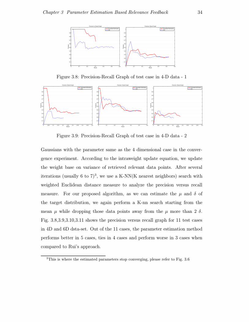
Fig. 3.8,3.9,3.10,3.11 shows the precision versus recall graph for 11 test cases
in 4D and 6D dsta-set. Out of the 11 cases, the parameter estimation method
performs better in 5 cases, ties in 4 cases and perform worse in 3 cases when
compared to Rui’s approach.
3This is where the estimated parameters stop converging, please refer to Fig. 3.6

Chapter 3 Parameter Estimation Based Relevance Feedback 35
0 0.1 0.2 0.3 0.4 0.5 0.60
0.1
0.2
0.3
0.4
0.5
0.6
0.7
0.8
0.9
1
Precision−Recall Graph
Recall
Pre
cisi
on
Parameter EstimationRUI
0 0.05 0.1 0.15 0.2 0.25 0.3 0.35 0.4 0.45 0.50
0.1
0.2
0.3
0.4
0.5
0.6
0.7
0.8
0.9
1
Precision−Recall Graph
Recall
Pre
cisi
on
Parameter EstimationRUI
0 0.1 0.2 0.3 0.4 0.5 0.60
0.1
0.2
0.3
0.4
0.5
0.6
0.7
0.8
0.9
1
Precision−Recall Graph
Recall
Pre
cisi
on
Parameter EstimationRUI
Figure 3.10: Precision-Recall Graph of test case in 6-D data - 1
0 0.1 0.2 0.3 0.4 0.5 0.60
0.1
0.2
0.3
0.4
0.5
0.6
0.7
0.8
0.9
1
Precision−Recall Graph
Recall
Pre
cisi
on
Parameter EstimationRUI
0 0.1 0.2 0.3 0.4 0.5 0.60
0.1
0.2
0.3
0.4
0.5
0.6
0.7
0.8
0.9
1
Precision−Recall Graph
Recall
Pre
cisi
on
Parameter EstimationRUI
0 0.1 0.2 0.3 0.4 0.5 0.60
0.1
0.2
0.3
0.4
0.5
0.6
0.7
0.8
0.9
1
Precision−Recall Graph
Recall
Pre
cisi
on
Parameter EsitmationRUI
Figure 3.11: Precision-Recall Graph of test case in 6-D data - 2
3.3.2 Performance Study in Intra- and Inter- Query Feed-
back
In this experiment, we work on the Corel image collection, which contains
40,000 images in different categories. Among the 400 categories, we selected
40 categories, each contains 100 images and ranges from the category of build-
ings, portrait, outdoor scenery, etc. We use the default groupings of im-
ages as the ground truth and human knowledge to run automated tests. We use
Color Moment and Cooccurence Matrix as the image features. Color Moment
computes the mean, variance and skewness values of each color channel in an
image. Cooccurence Matrix describes the texture of an image by measuring
the neighborhood pixel cooccurrence in the gray-level configurations.
The feature vectors of images are first extracted and normalized, then it is
used to train a 2D SOM structure of dimension 18×18. Queries are generated
and evenly distributed among the 40 classes, while the relevance feedbacks are

Chapter 3 Parameter Estimation Based Relevance Feedback 36
generated automatically based on the ground truth. All displayed images are
marked as relevant if they are in the same class as the query, and the others
are marked as non-relevant. The experiment is divided into 3 stages. In the
first stage, 160 queries (80 each) are simulated to find out the average recall
and precision when using the intra-weight updating version of Rui’s approach
and the intra-query approach in Section 3.2.4. In the second stage, a number
of queries are simulated and the SOM-based intra- and inter-query feedback
approach in Section 3.2.3 and 3.2.4 are both used to train the system and
retrieve images. In the final stage, 80 queries are simulated again to find out
the average recall and precision of our intra-query approach after inter-query
feedback is applied. Table 3.5 shows the parameters used in this experiment.
We then compare the result of Rui’s intra-weight approach and the intra-query
approach before and after our SOM-based inter-query feedback training.
Table 3.5: Parameters Used in Inter-Query Feedback ExperimentParameter Value
Number of images 4,000Number of categories 40Number of iterations usedin inter-query feedback 300,500Number of iterations usedin intra-query feedback 9Ratio of push αN and pull αR 20Feature used Color Moment (9-dimensions)
Cooccurence Matrix (20-dimensions)
Figure 3.12 shows the Recall-Precision graph, averaged among 80 queries,
of Rui’s approach and our approach before and after the SOM-based training.
We make two observations from the experiment. The first one is the intra-query
approach performs better after the SOM-based inter-query feedback training.
It shows that the retrieval precision can be improved by re-organizing the
feature vector space with SOM. The second one is Rui’s approach may perform
better than our intra-query approach initially, but when more relevant images
are retrieved, our performance on precision becomes better. It is because
our approach is target for estimating the distribution of the whole category

Chapter 3 Parameter Estimation Based Relevance Feedback 37
of relevant images instead of the distribution of relevant images around the
query; thus, when retrieving more images, its performance becomes better.
Moreover, the experiment indicates that the improvement is sensitive to the
push-pull value, their ratio and the number of iterations used in inter-query
feedback.
0 0.05 0.1 0.150.12
0.14
0.16
0.18
0.2300 iterations (pull=0.02, push=0.001)
Recall
Pre
cisi
on
Ruiw/o SOMw SOM
0 0.05 0.1 0.150.12
0.14
0.16
0.18
0.2500 iterations (pull=0.012, push=0.0006)
RecallP
reci
sion
Ruiw/o SOMw SOM
0 0.05 0.1 0.150.13
0.14
0.15
0.16
0.17
0.18
0.19
0.2300 iterations (pull=0.015, push=0.00075)
Recall
Pre
cisi
on
Ruiw/o SOMw SOM
0 0.05 0.1 0.150.13
0.14
0.15
0.16
0.17
0.18
0.19
0.2500 iterations (pull=0.012, push=0.0006)
Recall
Pre
cisi
on
Ruiw/o SOMw SOM
Color Moment Feature ( 9 − dimensions )
Cooccurence Matrix Feature ( 20 − dimensions )
Figure 3.12: Precision-Recall Graph Showing Performance in Real Data
3.4 Conclusion
In this section, we proposed an approach to estimate a user’s target distri-
bution through learning from his feedback via EM algorithm to be applied in
CBIR. We have verified the correctness and accuracy of this algorithm through
experiment on synthetic data. We proposed a display set selection strategy
that utilizes the information given by user in distinguishing image classes in
contrast to the K-NN approach for display set selection. Also, our method is
based on the parameter estimation of target distribution, we do not need to

Chapter 3 Parameter Estimation Based Relevance Feedback 38
perform a global update each image in the database accordingly. However, our
algorithm also has weaknesses. Since we need to accumulate 3 relevant data
points before starting the estimation, users might find this too long4. More-
over, maximum entropy strategy is used for display set selection, thus, user
might feel that the system cannot present the most relevant data during the
feedback process.
As the distribution of image classes in low-level feature space is not well
clustered, this makes the estimation of user’s target distribution difficult. In
the second part, we propose a SOM-based approach for re-organizing the fea-
ture space of images using inter-query feedback information. As a result, the
distribution of similar images more or less follows a Gaussian-like distribution
which make it more efficient for estimation. The proposed approach benefits
from reduced data-size and unchanged feature vector dimensionality compared
to existing inter-query feedback approaches. We demonstrate the improvement
in retrieval accuracy through experiments on real data.
4According to data shown in Fig. 3.7, this usually occur in the 2nd iteration

Chapter 4
DIStributed COntent-based
Visual Information Retrieval
4.1 Introduction
4.2 Peer Clustering
The design goal for our strategy is to improve data lookup efficiency in a
completely distributed P2P network, while keeping a simple network topology
and number of message passing to a minimum. In our proposed network, there
are two types of connections managed, namely random and attractive as
shown in Fig. 4.1. Random connections are to link peers randomly chosen
by the users. Attractive connections are to link peers sharing similar data
together. We perform clustering at the level of overlaying network topology
and also locally shared data, thus content-based query routing is realizable to
improve query efficiency. As a result, our algorithm manages to be scalable
when network grows. We have implemented a prototype version of DISCOVIR,
built on top of LimeWire [?] with content-based image searching capability and
improvement of data lookup efficiency.
39

Chapter 4 DIStributed COntent-based Visual Information Retrieval 40
Figure 4.1: Illustration of two types of connections in DISCOVIR.
4.2.1 Basic Version
In this section, we describe a restricted (yet effective and insightful) version
of our proposed algorithm to illustrate the idea of peer clustering. Consider
a P2P network consisting of peers sharing data of different interests as shown
in Fig. 4.2. In this network, shared data are classified into three different cat-
egories, which are (C)omputer, (H)istory, and (S)ociology respectively. Each
peer is represented by one of the three letters above to indicate the majority
of documents one shares, and we call this the signature value.
As shown in the example Fig. 4.2, a new peer of category (C)omputer C4
joins the network by connecting to a randomly selected peer S3, it sends out a
signature query to S3 and then propagates to S1 and H2 in the first hop, then,
to C1, C2, H1, S2 and S4 in the second hop and onwards. After collecting the
replies from other peers, peer C4 knows that C1, C2 and C3 share the same type
of documents (Computer) with it, thus, peer C4 makes an attractive connection
to either one of them; in this example, C3 is chosen. As the network grows,
we envison a clustered P2P network is formed. Referring to Fig. 4.2, all peers
with the same signature value are interconnected by attractive connections, a
query routing scheme thus can be applied.
Let us assume the new user, peer C4, wants to find some documents under
the category (H)istory, it initiates a query and checks against its signature

Chapter 4 DIStributed COntent-based Visual Information Retrieval 41
value. It finds that the query mismatches with its signature value, thus the
query is forwarded through random connection to S3. S3 receives the query
and performs the same checking. It finds that the query and its signature
value are still mismatched, it continue to forward the query through random
connection to H2. Once H2 receives this query, it checks against its signature
value and finds the query reached the target cluster. Therefore, it broadcasts
the query inside the cluster through attractive connection to H1. Likewise,
when H1 receives the query, it propagatess the query to H3, and so on. Under
this selective query routing scheme, we avoid the query to pass through some
unrelated peers. The number of query messages used is reduced while query
is still able to reach peers containing the answer.
The detailed description and analysis of this algorithm was proposed in [25],
which shows promising result against the conventional Gnutella query mecha-
nism. As this version of peer clustering requires users to assign signature value
to a peer and agree upon a set of categories in the distributed P2P environ-
ment, which is not practical enough to be applied in an open environment,
we propose two enhanced versions based on this foundation in the next two
sections.
Figure 4.2: Peer Clustering - Basic Version
Chapter 4 DIStributed COntent-based Visual Information Retrieval 42
4.2.2 Single Cluster Version
Since peer clustering based on the category of shared documents stated by the
user explicitly is not practical enough as aforementioned, we move on to peer
clustering based on content feature of shared documents. In the information
retrieval literature, text documents and images are processed to use feature
vectors as their representation, while similarity between two documents are
distance measure in the vector space. Clustering in the vector space had
been vastly studied to improve retrieval performance by serving as an indexing
structure. We surmise such techniques is alo valuable to a P2P Distributed
Envrionemnt in improving the performance.
In the following, we apply notation in graph theory to model the DIS-
COVIR network (see Table. 4.1). For the sake of generality, we try to keep
this in high level of abstraction. In this version of peer clustering algorithm, we
choose the mean and standard deviation of cluster as signature value of peers,
while Euclidean distance is used for similarity measure. In the actual real-
ization, we choose image feature vector as the data structure for representing
images, which give birth to the name of our system DISCOVIR (DIStributed
COntent-based Visual Information Retrieval). Here are some definitions:
Definition 1 We consider files shared by a peer can be represented in multi-
dimension vectors based on its content, and the similarity among files is based
on the distance measure between vectors. Consider
f : cv → ~cv (4.1)
f : q → ~q (4.2)
f is the mapping function from file cv to a vector ~cv. In the notion of image
processing, cv is the raw image data, f is a specific feature extraction method,

Chapter 4 DIStributed COntent-based Visual Information Retrieval 43
Table 4.1: Definition of TermsG{V,E} The P2P network, with V denoting the set of peers and E
denoting the set of connection
E = {Er, Ea} The set of connections, composed of random connections,Er and attractive connections, Ea.
ea = (v, w, The attractive connection between peers v, w based onsigv, sigw), sigv and sigwv, w ∈ V, ea ∈ Ea
|V | Total number of peers.
|E| Total number of connections.
Horizon(v, t) ⊆ V Set of peers reachable from v within t hops
SIGv , v ∈ V Set of signature values characterizing the data shared bypeer v
D(sigv , sigv), Distance measure between specific signature values of twov, w ∈ V peers v and w
Sim(sigv , q) Similarity measure between a query qsigv ∈ SIGv and peer v based on sigv.
C = {Cv : v ∈ V } The collection of data shared in the DISCOVIR network.
Cv The collection of data shared by peer v, which is a subsetof C.
REL(cv , q), A function determining relevance of data cv to a query q.cv ∈ Cv 1-relevant, 0-non-relevant
~cv is the extracted feature vector characterizing the image. Likewise, f is also
used to map a query q to a query vector ~q, to be sent out when user makes a
query by example1.
Definition 2 sigv is the signature values representing characteristic of data
1In Content-based Image Retrieval, users usally provide an example images or a sketchto search for similar images

Chapter 4 DIStributed COntent-based Visual Information Retrieval 44
shared by peer v. We define
sigv = (~µ,~δ), (4.3)
where ~µ and ~δ are the statistical mean and standard deviation of the collection
of data in their feature vector space, belonging to peer v, From now on, sigv
characterizes the data shared by peer v.
Definition 3 D(sigv, sigw) is defined as the distance measure between sigv
and sigw, in other sense, the similarity between two different peers v and w.
It is defined as,
D(sigv, sigw) = || ~µv − ~µw||. (4.4)
|| ~µv − ~µw|| is the Euclidean distance between two centroids symbolized by
sigv, sigw. We define the data similarity of two peers by this formula and use
it to help organizing the network.
Based on the above definitions, we introduce a peer clustering algorithm,
to be used in the network setup stage, in order to help building the DISCOVIR
as a self-organized network oriented in content similarity. It consists of three
steps as follows:
1. Signature Value Calculation–Every peer preprocesses its data collec-
tion and calculates signature values sigv to characterize its data prop-
erties by assuming all feature vectors as a single cluster. Whenever the
shared data collection, Cv, of a peer changes, the signature value is up-
dated accordingly.
2. Neighborhood Discovery–After a peer joins the DISCOVIR network
by connecting to a random peer in the network, it broadcasts a signa-
ture query message, similar to that of ping-pong messages in Gnutella,
to ask for signature value of peers within its neighborhood, sigw, w ∈

Chapter 4 DIStributed COntent-based Visual Information Retrieval 45
Horizon(v, t). This task is not only done when a peer first joins the
network, it repeats every certain interval in order to maintain the latest
information of other peers.
3. Attractive Connection Establishment–After acquiring the signature
values of other peers, one can reveal the peer with signature value closest
to its according to definition 3, and make an attractive connection to link
them up. This attractive connection is reestablished to the second closest
one in the host cache2 whenever current connection breaks.
Fig 4.2.2 illustrate a working example of peer clustering model. The number
of each node indicates their time of appearance in the DISCOVIR network, 1
being the oldest node and 11 being the newest node. the (x, y) value besides
a node is its signature value in 2-D feature vector space. Table 4.2 is a matrix
showing the pair-wise distance of signature values among the peers. When peer
11 joins the network, it first connect to peer 9 by a random connection. It sends
out a signature value query message to peer 9; after that, it turns out that
peer 10 is closest to peer 11 in the sense of distance in signature value. Peer
11 the make an attractive connection to peer 10. Having all peers joining the
DISCOVIR network perform the three tasks described above, you can envision
a P2P network with self-organizing ability to be constructed. Peers sharing
similar content will be grouped together like a Yellow Pages. The detail steps
of peer cluster is illustrated in Algorithm 1. depicts the peer clustering.
Algorithm 1 Algorithm for Peer Clustering - Single Cluster Version
Peer-Clustering(peer v, integer ttl)for all w ∈ Horizon(v, t) do
Compute D(sigv, sigw)end forEa = Ea ∪ (v, w, sigv, sigw) having min(D(sigv, sigw))
2The host cache is obtained from the Neighborhood Discovery stage

Chapter 4 DIStributed COntent-based Visual Information Retrieval 46
9
1
7
8
5
3
10
11
New attractive connection
Random connection
2
4
6
Existing clustered P2P network
(1.5,1.2)
(1.3,2.4)
(1.6,1.8)
(5.2,8.5)
(5.6,8.8)
(4.9,9.7)
(4.7,9.3)
(2.9,6.5)
(2.7,6.0) (2.6,5.9)
(2.0,5.8) Random connection Attractive connection
( x,y ) Signature value
Figure 4.3: Peer Clustering - Single Cluster Version
Table 4.2: Distance Between Signature Values of Peerspeer 1 2 3 4 5 6 7 8 9 10 11
1 0.00 8.18 7.24 3.68 0.94 1.24 4.19 7.61 0.50 3.54 3.052 0.00 1.22 4.83 8.71 9.15 4.63 0.61 8.64 4.95 5.483 0.00 3.73 7.69 8.14 3.47 0.67 7.70 3.86 4.404 0.00 4.0 4.44 0.61 4.22 4.17 0.14 0.675 0.00 0.45 4.42 8.12 1.03 3.86 3.336 0.00 4.86 8.56 1.14 4.3 3.777 0.00 4.02 4.69 0.73 1.148 0.00 8.06 4.34 4.889 0.00 4.1 3.5510 0.00 0.5411 0.00
4.2.3 Multiple Clusters Version
The previous version of peer clustering assumes most of the data shared by
a peer fall in the same category, e. g. , a peer shares collection of sunset
images or collection of computer science paper, thus the extracted feature
vectors will be clustered together and one signature value is able to describe
the data characteristic reasonably. However, most user share documents of
various topics in real-world situation as shown in Fig. 4.4, there should be an
attractive connection between sub-cluster A2 of peer A and sub-cluster B3 of
peer B although their cluster centroid are far apart.
We propose to use multiple signature values sigv, sigv ∈ SIGv to represent
a peer because the document collection is likely to fall into several categories
and their extracted feature vectors form several clusters as well. With these

Chapter 4 DIStributed COntent-based Visual Information Retrieval 47
changes, peers may form several attractive connections depending on the num-
ber of local sub-clusters. The revised algorithm is illustrated in Algorithm 2
and two changes in the main steps are updated as follows:
1. Signature Value Acquisition–In the preprocessing stage, a set of sig-
nature values SIGv is calculated, which are the statistical mean and
standard deviation of sub-clusters found using some clustering algorithm
like k-means [1], competitive learning [33], or expectation maximization
[10]. The number of signature values is variable and it is a trade-off
between resolution of cluster and computational cost. In the
DISCOVIR, we choose competitive learning and three as the number of
signature values in a peer for the sake of low computation cost.
2. Attractive Connection Establishment–This process is the same as
that in previous section except we make attractive connection for every
signature values a peer possess. The standard deviation of a signature
value is reserved to control the quality of attractive connections, the
smaller the standard deviation, the better to make attractive connection
because it implies a dense cluster.
We have introduced the final and most practical version of peer clustering
algorithm in DISCOVIR, having all peers follow this procedure to build the
network, a self-organizing network is formed, we delineate a selective query
routing strategy in the next section to improve retrieval performance.
4.3 Firework Query Model
To make use of our clustered P2P network, we propose a content-based query
routing strategy called Firework Query Model (FQM). In this model, a query
message is routed selectively according to the content of the query. Once
it reaches its designated cluster, the query message is broadcasted by peers

Chapter 4 DIStributed COntent-based Visual Information Retrieval 48
Figure 4.4: Multiple Clusters Exist in a Peer.
Algorithm 2 Algorithm for Peer Clustering - Multiple Clusters Version
Peer-Clustering(peer v, integer ttl)for all sigv ∈ SIGv do
for all w ∈ Horizon(v, t) dofor all sigw ∈ SIGw do
Compute D(sigv, sigw)end for
end forEa = Ea ∪ (v, w, sigv, sigw) having min(D(sigv, sigw))
end for
through the attractive connections inside the cluster much like an exploding
firework as shown in Fig. 4.5. Our strategy aims to:
1. Minimize the number of messages passing through the overlay network,
2. Reduce the workload of each computer, and
3. Maximize the number of relevnat documents retrieved from the peer-to-
peer network.
Here, we introduce the algorithm to determine when and how a query
message is propagated like a firework in Algorithm 3. When a peer receives
the query, it carries out two steps:
1. Shared File Look Up–The peer looks up its shared information for
those matched with the query. Let q be the query, and ~q be its vector

Chapter 4 DIStributed COntent-based Visual Information Retrieval 49
Figure 4.5: Illustration of firework query.
representation, REL(cv, q) is the relevance measure between the query
and the file cv shared by peer v, it depends on a L2 norm defined as,
REL(cv, q) =
1 ||~cv − ~q|| ≤ T
0 ||~cv − ~q|| > T,
where T is a threshold defining the degree of result similarity a user
wants.If it is larger, then more result will be obtained (but no guarantee
to maintain high precision). If any shared documents within the match-
ing criteria of the query, the peer will reply the requester. In addition, we
can reduce the number of REL(cv, q) computations by performing local
clustering3 in a peer, thus speeding up the process of query response.
2. Route Selection–The peer calculates the similarity between the query
and each signature value of its local clusters, sigv , which is represented
as,
Sim(sigv, q) =d∏
i
1√2πδi
e− (qi−µi)2
2δ2i , sigv = (~µ,~δ), (4.5)
where i is the index of dimension of feature vector. If none of the distance mea-
sure between its local clusters’ signature value and the query, Sim(sigv, q), is
3We compare query to sub-clusters first instead of comparing with each documents
Chapter 4 DIStributed COntent-based Visual Information Retrieval 50
larger than a preset threshold, θ, the peer will propagate the query to its neigh-
bors through random connections. Otherwise, if one or more Sim(sigv, q) is
larger than the threshold, it implies the query has reached its target clus-
ter. Therefore, the query will be propagated through corresponding attractive
connections much like an exploding firework.
In our model, we retain two existing mechanisms in Gnutella network
for preventing query messages from looping forever in the distributed net-
work, namely, the Gnutella replicated message checking rule and Time-To-
Live (TTL) of messages. When a new query appears to a peer, it is checked
against a local cache for duplication. If it is found that the same message has
passed through before, the message will not be propagated4. The second mech-
anism is to use the Time-To-Live value to indicate how long a message can
survive. Similar to IP packets, every Gnutella messages are associated with
a TTL. Each time when the message passes through a peer, the TTL value
is decreased by one. Once the TTL is zero, the message will be dropped and
no longer forwarded. There is a modification on DISCOVIR query messages
from the original Gnutella messages. In our model, the TTL value is decre-
mented by one with a different probability when the message is forwarded
through different types of connection5. For random connections, the probabil-
ity of decreasing TTL value is 1. For attractive connections, the probability of
decreasing TTL value is an arbitrary value in [0, 1] called Chance-To-Survive
(CTS). This strategy can reduce the number of messages passing outside the
target cluster, while more relevant information can be retrieved inside the
target cluster because the query message has a greater chance to survive de-
pending on the CTS value. In particular, we choose CTS=0 in our simulation
experiment.
4This is realized by generating a Globally Unique ID GUID for every message sent out.5Similar method of propagating queries with different probability was studied in [3] from
the percolation theory perspective.

Chapter 4 DIStributed COntent-based Visual Information Retrieval 51
Algorithm 3 Algorithm for the Firework Query Model
Firework-query-routing (peer v, query q)for all sigv ∈ SIGv do
if Sim(sigv, q) > θ (threshold) thenif rand() > CTS thenqttl = qttl − 1
end ifif qttl > 0 then
propagate q to all ea(a, b, c, d) where a = v, c = sigv or b = v, d = sigv(attractive link)
end ifend if
end forif Not forwarding to attractive link thenqttl = qttl − 1if qTTL > 0 then
forward q to all er(a, b) where a = v or b = v (random link)end if
end if
4.4 Implementation and System Architecture
We briefly outline the process of sharing and retrieving image in DISCOVIR.
First, each peer is responsible to perform feature extraction, e.g., color, tex-
ture, shape, etc, on its shared images in each peer using the DISCOVIR client
program. With this program, each peer maintains its local index of feature
vectors of its image collection. When a peer, the requester, initiates a query
by giving an example image and a particular feature extraction method, it
performs feature extraction on the example image and sends the feature vec-
tor, contained in a query message, to all its connecting peers. Consequently,
other peers compare this query to their feature vector index. Based on a dis-
tance measure, they find a set of similar images and return results back to the
requester. Likewise, these peers will propagate the query to their connecting
peers and this process continues to query other peers in a large portion of the
network.

Chapter 4 DIStributed COntent-based Visual Information Retrieval 52
DISCOVIR uses a plug-in architecture to support different feature extrac-
tion method. User may select to download a plug-in in the format of compiled
Java bytecode if they want to perform CBIR based on that particular feature
extraction method. The following is a screen capture of the DISCOVIR client
program, see Fig. 4.6, which can be downloaded from the site [22]. In the
following, we describe the overall architecture of DISCOVIR, which operates
on the current Gnutella network, and the modification of query messages.
Figure 4.6: Screen-shot of DISCOVIR.
4.4.1 Gnutella Message Modification
The DISCOVIR system is compatible to the Gnutella (v0.4) protocol [13].
In order to support the image query functionalities mentioned, two types of
messages are added. They are:
• ImageQuery - Special type of the Query message. It is to carry name of
feature extraction method and feature vector of query image, see Fig. 4.7.
• ImageQueryHit - Special type of the QueryHit message. It is to re-
spond to the ImageQuery message, it contains the location, filename and

Chapter 4 DIStributed COntent-based Visual Information Retrieval 53
size of similar images retrieved, and their similarity measure to the query.
Besides, the location information of corresponding thumbnails are added
for the purpose of previewing result set in a faster speed, see Fig. 4.8.
Figure 4.7: ImageQuery Message Format
Figure 4.8: ImageQueryHit Message Format
4.4.2 Architecture of DISCOVIR
In this section, we describe the architecture of a DISCOVIR client and the
interaction within modules in order to perform CBIR over a P2P network.
Figure 4.9 depicts the key components and their interaction in the architecture
of a DISCOVIR client. As DISCOVIR is built based on the LimeWire [?]
open source project, the operations of Connection Manager, Packet Router and
HTTP Agent remain more or less the same with some additional functionalities
to improve the query mechanism used in original Gnutella network. The Plug-
in Manager, Feature Extractor and Image Indexer are introduced to support
the CBIR task. The User Interface is modified to incorporate the image search
panel. Figure 4.6 shows a screen capture of DISCOVIR in the image search
page. Here are brief descriptions of the six major components:
• Connection Manager - It is responsible for setting up and managing
the TCP connection between DISCOVIR clients.

Chapter 4 DIStributed COntent-based Visual Information Retrieval 54
Connection Manager
Packet Router
Plug - in Manager
HTTP Agent
Feature Extractor
Image Indexer
DISCOVIR Network Shared Collection
DISCOVIR Core
DISCOVIR User Interface
WWW
Image Manager
Figure 4.9: Architecture of DISCOVIR.
• Packet Router - It controls the routing, assembling and disassembling
of message between DISCOVIR network and components in a peer.
• Plug-in Manager - It coordinates the download and storage of different
feature extraction plug-ins and their interaction with Feature Extractor
and Image Indexer.
• HTTP Agent - It is a tiny web-server that handles file download request
from other DISCOVIR peers using HTTP protocol.
• Feature Extractor - It collaborates with the Plug-in Manager to per-
form various feature extraction and thumbnail generate of the shared
image collection. It involves in two main functions:
– Preprocessing - It extracts the feature vector of shared images in
order to make the collection searchable in the network.
– Real Time Extraction - It extracts the feature vector of query
image on-the-fly and passes the query to Packet Router.
• Image Indexer - It indexes the image collection by content feature and
carries out clustering to speed up the retrieval of images.

Chapter 4 DIStributed COntent-based Visual Information Retrieval 55
4.4.3 Flow of Operations
The four main steps of performing CBIR in DISCOVIR are listed in detail as
follows.
1)Preprocessing
The Plug-in Manager module is responsible for contacting the DISCOVIR
control website to inquire the list of available feature extraction modules. It
will download and install selected modules upon user’s request. Currently,
DISCOVIR supports various feature extraction methods in color and texture
categories such as AverageRGB, GlobalColorHistogram, ColorMoment, Co-
occurrence matrix, etc. All feature extraction modules strictly follow a prede-
fined API in order to realize the polymorphic properties of switching between
different plug-ins dynamically.
The Feature Extractor module extracts feature and generates thumbnails
for all shared images using a particular feature extraction method chosen by
user. The Image Indexer module then indexes the image collection using the
extracted multi-dimensional feature vectors. Compared with the centralized
web-based CBIR approach, sharing the workload of this computational costly
task among peers by allowing them to store and index their own image collec-
tion helps to solve the bottle-neck problem by utilizing distributed computing
resources.
2)Connection Establishment
For a peer to join the DISCOVIR network, the Connection Manager module
asks the Bootstrap Server, which is program storing and answering a list of
peers currently in the network, for peers available for accepting income con-
nection. Once the IP address is known, the peer hooks up to the DISCOVIR
network by connecting to currently available peers.

Chapter 4 DIStributed COntent-based Visual Information Retrieval 56
3)Query Message Routing
When a peer initiates a query for similar images, the Feature Extractor module
processes the query image instantly and assemble an ImageQuery message, as
shown in Fig. 4.7, to be sent out through Packet Router module. Likewise,
when other peers receive the ImageQuery messages, they need to perform two
operations, Query Message Propagation and Local Index Look Up.
• Query Message Propagation - When propagating the query mes-
sage, the Packet Router module of DISCOVIR employs two checking
rules adopted from Gnutella network. In order to prevent messages from
looping forever in the DISCOVIR network, they are (1) Gnutella repli-
cated message checking rule and (2) Time-To-Live (TTL) of messages
respectively. The replicated message checking rule prevents a peer from
propagating the same query message again. The TTL mechanism con-
strains the reachable horizon of a query message.
• Local Index Look Up - The peer searches its local index of shared
files for similar images using the Image Indexer module and information
in the ImageQuery message. Once similar images are retrieved, the peer
delivers an ImageQueryHit message, see Fig. 4.8, back to the requester
through Packet Router module.
4)Query Result Display
When an ImageQueryHit message returns to the requester, user will obtain a
list detailing the location and size of matched images. In order to retrieve the
query result, the HTTP Agent module downloads thumbnails, generated in
the preprocessing stage, or full size image from the peer using HTTP protocol.
On the other hand, HTTP Agent module in other peers serve as a web server
to deliver the requested images.

Chapter 4 DIStributed COntent-based Visual Information Retrieval 57
4.5 Experiment
In this section, we discuss the design of simulation experiments and evaluate
the performance of our proposed Peer Clustering and Firework Query Model.
First, we present our model of Peer-to-Peer network used in our simulation
and introduce the performance metrics used for evaluation in section 4.5.1. We
study the performance of FQM using different parameters, with the experiment
on number of peers in section ?? and the experiment on TTL of query message
in section ??. We show how our strategy performs, behaves at scale and give
final remarks at the end.
4.5.1 Simulation Model of the Peer-to-Peer Network
Our goal of the experiment is to model a typical Peer-to-Peer network of nodes
T where each node contains a set of documents. We built different size of
P2P networks to evaluate the performance of different search mechanisms.
As shown in figure 4.5, the network follows a power law distribution with an
average degree of 3.97 when the number of peers is 8000. The number of peers
in each network varies from 2000 to 20000. The diameter6 varies from 9 to 11,
and the average distances7 between two peers vary from 5.36 to 6.58. Table. 4.3
lists the detailed information of each model.
Table 4.3: Characteristics of Each P2P Network ModelNumber of Peer 2000 4000 8000 12000 16000 20000
Diameter 9 9 10 10 11 11
Average distance between two peers 5.36 5.77 6.12 6.33 6.47 6.58
The simulations are done over different network configurations and data
placement methods. We run 100 iterations and average the results for each set
of parameters. For every 10 iterations, we rebuild the simulated network again,
6It is the largest number of hops among the shortest path between any pairs of peers.7The average shortest path between any pairs of peers.
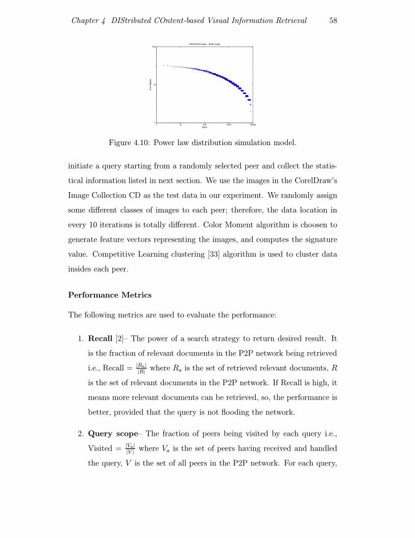
Chapter 4 DIStributed COntent-based Visual Information Retrieval 58
1 10 100 1000 100001
10
100DISCOVIR Graph − 8000 nodes
Rank
Out
−deg
ree
Figure 4.10: Power law distribution simulation model.
initiate a query starting from a randomly selected peer and collect the statis-
tical information listed in next section. We use the images in the CorelDraw’s
Image Collection CD as the test data in our experiment. We randomly assign
some different classes of images to each peer; therefore, the data location in
every 10 iterations is totally different. Color Moment algorithm is choosen to
generate feature vectors representing the images, and computes the signature
value. Competitive Learning clustering [33] algorithm is used to cluster data
insides each peer.
Performance Metrics
The following metrics are used to evaluate the performance:
1. Recall [2]– The power of a search strategy to return desired result. It
is the fraction of relevant documents in the P2P network being retrieved
i.e., Recall = |Ra||R| where Ra is the set of retrieved relevant documents, R
is the set of relevant documents in the P2P network. If Recall is high, it
means more relevant documents can be retrieved, so, the performance is
better, provided that the query is not flooding the network.
2. Query scope– The fraction of peers being visited by each query i.e.,
Visited = |Va||V | where Va is the set of peers having received and handled
the query, V is the set of all peers in the P2P network. For each query,

Chapter 4 DIStributed COntent-based Visual Information Retrieval 59
if the fraction of involved peers in the network is lower, the system will
be more scalable, provided that a significant amount of desired result is
retrieved.
3. Query efficiency– The ratio between the Recall and Query Scope i.e.,
Efficiency = RecallQuery Scope . The performance is more desirable if we can
retrieve more relevant documents but only visited fewer peers. If the
data placement are evenly distributed and the inherent Gnutella search
mechanism is used, the Query Efficiency is equal to 1. In other words,
the more peers a query visited, the more relevant result retrieved.
4. Generated network traffic– The number of packets generated for each
query. Reducing the load at individual peers and network traffic is de-
sirable for scalability, This is in proportion to the Query Scope.
5. Minimum reply path length– Reply path length is the number of hops
from query requester to a peer that replies the query.In our experiments,
it is defined as the average number of hops for first ten replies. It is more
desirable if the minimum reply path length is shorter. The requester can
receive the reply in a shorter time.
4.5.2 Number of Peers
This experiment tests the scalability of search mechanisms. The number of
peers in each network varies from 2000 to 20000. The experiment parameters
are listed in Table. 4.4.
Recall
Figure 4.11 depicts the recall against number of peers in two search mecha-
nisms. When the size of network increases, the recall of Firework Query Model
continues to remain at a higher range, while the recall for BFS drops when size

Chapter 4 DIStributed COntent-based Visual Information Retrieval 60
Table 4.4: Experiment Parameters for Scalability ExperimentNumber of Peer 2000 - 20000Topology if the P2P network Power law distribution with an
average branching degree of 3.97Diameter of the P2P network 9 - 11 hopsAverage distance between 2 peers 5.4 - 6.6 hopsNumber of documentsassigned to each peer 200 - 400 documentsDimension of extracted featurevector to represent the image 9TTL value of the query packet 5
of network grows. We conclude that our algorithm is insensitive to the change
of network size. Our mechanism is more scalable. Even the size of network
grows, FQM still can reach a large portion of the network containing the query
target.
0 0.2 0.4 0.6 0.8 1 1.2 1.4 1.6 1.8 2 2.2
x 104
0
0.1
0.2
0.3
0.4
0.5
0.6
0.7
0.8
0.9
1
Number of peers
Rec
all
BFSFQM
Figure 4.11: Recall against Number of Peers
Query scope
As seen in Figure 4.12, we achieve the load reduction by using FQM. Fewer
peers are exposed to each query.
0 0.2 0.4 0.6 0.8 1 1.2 1.4 1.6 1.8 2 2.2
x 104
0
0.1
0.2
0.3
0.4
0.5
0.6
0.7
0.8
0.9
1
Number of peers
Que
ry S
cope
BFSFQM
Figure 4.12: Query scope against Number of Peers

Chapter 4 DIStributed COntent-based Visual Information Retrieval 61
Query Efficiency
As seen in Figure 4.13, FQM outperforms BFS. The efficiency is improved
more than 60%. The curve of FQM follows a small bell shape. Query efficiency
increases at first due to two reasons:
0 0.2 0.4 0.6 0.8 1 1.2 1.4 1.6 1.8 2 2.2
x 104
0
0.2
0.4
0.6
0.8
1
1.2
1.4
1.6
1.8
2
Number of peers
Que
ry E
ffici
ency
BFSFQM
Figure 4.13: Query Efficiency against Number of Peers
1. The network can be clustered more appropriately when the network size
increases. When the number of peers increases, new peers can have more
choices and make their attractive link to a more similar peer.
2. The percentage of peers visited is inversely proportional to the network
size when the TTL is fixed. FQM advances the recall percentage when
the query message reaches the target cluster.
When the network size increases further, a query might not reach its target
cluster for low TTL value (The TTL is fixed to 5 in this experiment and the
diameter increases from 9 to 11), so query efficiency starts to drop. Therefore,
choosing a good TTL value is important in our algorithm and this will be
discussed in the next section.
Generated network traffic
Our proposed Firework Query Model reduces the generated traffic by routing
the query selectively rather than broadcasting. Figure 4.14 shows the average
number of packets generated.

Chapter 4 DIStributed COntent-based Visual Information Retrieval 62
2000 4000 8000 12000 16000 200000
5000
10000
15000
Number of peers
Num
ber
of q
uery
pac
kets
gen
erat
ed
Figure 4.14: Generated network traffic against Number of Peers
Minimum reply path length
Figure 4.15 depicts the minimum reply path length of the average number of
hops for first ten replies. On average, the relevant documents are 3-7 hops
away in Brute Force Search algorithm, however, the path length in Firework
Query Model is just 2-5 hops. It is more desirable if the minimum reply path
length is shorter. The requester can receive the reply in a shorter time and
the system is also more scalable.
2000 4000 8000 12000 16000 200000
1
2
3
4
5
6
7
8
Number of peers
Min
imum
rep
ly p
ath
lebg
th
Figure 4.15: Minimum reply path length against Number of Peers
4.5.3 TTL of Query Message
In this section, we explore how the performances are affected by different Time-
To-Live (TTL) values of query packet. The number of peers in each network is
fixed to 10000. The TTL value varies from 4 to 8. The experiment parameters
are listed in Table. 4.5.

Chapter 4 DIStributed COntent-based Visual Information Retrieval 63
Table 4.5: Experiment parametersNumber of Peer 10000Topology if the P2P network Power law distribution with an
average branching degree of 3.97Diameter of the P2P network 10 hopsAverage distance between 2 peers 6.2 hopsNumber of documentsassigned to each peer 200 - 400 documentsDimension of extracted featurevector to represent the image 9TTL value of the query packet 4 - 8
Query Efficiency
As seen in Figure 4.16, FQM outperforms BFS under different TTL values of
query packet. We found that the optimal TTL value is 7 in a network size of
ten thousands peers under Firework Query Model. The Query Efficiency is low
at the beginning because the TTL value is not enough for the query packet to
reach its target cluster. When the TTL value increase, the query has a larger
chance to reach its target cluster, therefore, the Query Efficiency increases.
When the TTL value is 7, the Query Efficiency is optimal because the query
packet can just reach its target cluster. However, further increasing the TTL
value will only generate unnecessary traffic, therefore, the Query Efficiency
starts to drop when TTL is 8.
3.5 4 4.5 5 5.5 6 6.5 7 7.5 8 8.50
0.5
1
1.5
2
TTL of query packet
Que
ry E
ffici
ency
BFSFQM
Figure 4.16: Query Efficiency against TTL value of query packet

Chapter 5
Future Works and Conclusion
64

Appendix A
Efficient Discovery of Signature
Value
I will add a description of how to discover the signature values of neighboring
peers efficiently.
65

Bibliography
[1] M. R. Anderberg. Cluster analysis for applications. In Academic Press,
New York, 1973.
[2] Ricardo Baeza-Yates and Berthier Ribeiro-Neto. Modern Information Re-
trieval. ACM Press, Addison Wesley, 1999.
[3] Farnoush Banaei-Kashani and Cyrus Shahabi. Criticality-based Analy-
sis and Design of Unstructured Peer-to-Peer Networks as ”Complex Sys-
tems”. In Proceedings of the Third International Workshop on Global and
Peer-to-Peer Computing (G2P2PC), 2003.
[4] Michael Bergman. The deep web: Surfacing hidden value. Website,
http://www.brightplanet.com/deepcontent/, September 2001.
[5] Wendy Chang, Gholamhosein Sheikholeslami, Jia Wang, and Aidong
Zhang. Data Resource Selection in Distributed Visual Information Sys-
tems. IEEE Transactions on Knowledge and Data Engineering, 10(6):926–
946, November/December 1998.
[6] George Coulouris, Jean Dollimore, and Tim Kindberg. Distributed Sys-
tems Concepts and Design. Addison-Wesley, third edition, 2001.
[7] Ingemar J. and Cox. The bayesian image retrieval system, pichunter, the-
ory, implementation, and psychophysical experiments. IEEE Transactions
on Image Processing, 9(20-37), January 2000.
66

[8] Arturo Crespo and Hector Gracia-Molina. Routing Indices For Peer-to-
Peer Systems. In Proceedings of the Internation Conference on Distributed
Computing Systems (ICDCS), July 2002.
[9] Scott C. Deerwester, Susan T. Dumais, Thomas K. Landauer, George W.
Furnas, and Richard A. Harshman. Indexing by Latent Semantic Analysis.
Journal of the American Society of Information Science, 41(6):391–407,
1990.
[10] A.P. Dempster, N.M. Laird, and Rubin D.B. Maximum likelihood from
incomplete data via the EM algorithm. J. R. Statist. Soc. B, 39:185–197,
1977.
[11] C. Faloutsos, R. Barber, M. Flickner, J. Hafner, Niblack W., D. Petkovic,
and W. Equitz. Efficient and effective querying by image content. Journal
of Intelligent Information Systems: Integrating Artificial Intelligence and
Database Technologies, 3(3-4):231–262, 1994.
[12] The freenet homepage. http://freenet.sourceforge.net.
[13] The gnutella homepage. http://www.gnutella.com.
[14] Xiaofei He, Oliver King, Wei-Ying Ma, Mingjing Li, and Hong-Jiang
Zhang. Learning a Semantic Space From User’s Relevance Feedback for
Image Retrieval. IEEE Transactions on Circuits and Systems for Video
Technology, 13(1), January 2003.
[15] Douglas R. Heisterkamp. Building a Latent Semantic Index of an Image
Database from Patterns of Relevance Feedback. In Proceedings of the
16th International Conference on Pattern Recognition (ICPR 2002), pages
134–137, August 2002.
[16] Irwin King and Zhong Jin. Relevance feedback content-based image re-
trieval using query distribution estimation based on maximum entropy
67

principle. In Liming Zhang and Fanji Gu, editors, Proceedings to the In-
ternational Conference on Neural Information Processing (ICONIP2001),
volume 2, pages 699–704, Shanghai, China, November 14-18 2001. Fudan
University, Fudan University Press.
[17] Teuvo Kohonen. Self-Organizing Maps, volume 30 of Springer Series in
Information Sciences. Springer, third edition, 2001.
[18] T. K. Lau and I. King. Montage: An image database for the fash-
ion, clothing, and textile industry in Hong Kong. In Proceedings of the
Third Asian Conference on Computer Vision (ACCV’98), volume 1351
of Lecture Notes in Computer Science, pages I 410–417. Berlin, Germany:
Springer Verlag, January 4-7, 1998.
[19] Steve Lawrence and C. Lee Giles. Searching the World Wide Web. Science,
280(5360):98–100, 1998.
[20] Modern peer-to-peer file-sharing over the internet.
http://www.limewire.com/index.jsp/p2p.
[21] S. Mehrotra, Y. Rui, M. Ortega, and T.S. Huang. Supporting content-
based queries over images in mars. In Proc. IEEE Int. Conf. Multimedia
Computing and Systems, pages 632–633, 1997.
[22] Multimedia Information Processing Lab - CUHK.
http://www.cse.cuhk.edu.hk/∼miplab.
[23] The napster homepage. http://www.napster.com.
[24] A. Natsev, R. Rastogi, and K. Shim. Walrus: A similarity retrieval algo-
rithm for image databases. In Proc. SIGMOD, Philadelphia, PA, 1999.
68

[25] Cheuk Hang Ng and Ka Cheung Sia. Peer Clustering and Firework Query
Model. In Poster Proc. of The 11th International World Wide Web Con-
ference, May 2002.
[26] K. Nigam, A. McCallum, S. Thrun, and T. Mitchell. Text classification
from labeled and unlabeled documents using em, 1999.
[27] A. Pentland, R. W. Picard, and S. Sclaroff. Photobook: tools for content-
based manipulation of image databases. In Proc. SPIE, volume 2185,
pages 34–47, February 1994.
[28] S. Ratnasamy, P. Francis, M. Handley, and S. Karp R. Shenker. A scalable
content-addressable network. In In Proc. ACM SIGCOMM, August 2001.
[29] Sylvia Ratnasamy, Scott Shenker, and Ion Stoica. Routing algorithms for
DHTs: Some open questions. In Proceedigns of the International Peer-to-
Peer Workshop, 2002.
[30] Antony Rowstron and Peter Druschel. Pastry: Scalable, decentralized
object location and routing for large-scale peer-to-peer systems. In Pro-
ceedings of the 18th IFIP/ACM International Conference on Distributed
Systems Platforms, November 2001.
[31] Yong Rui, Thomas S. Huang, and Shih-Fu Chang. Image retrieval: cur-
rent techniques, promising directions and open issues. Journal of Visual
Communication and Image Representation, 10:39–62, April 1999.
[32] Yong Rui, Thomas S. Huang, Michael Ortega, and Sharad Mehrota. Rel-
evance feedback: A power tool for interactive content-based image re-
trieval. IEEE Transactions on Circuits and Video Technology, 8(644-655),
September 1998.
[33] D.E. Rumelhart and D. Zipser. Feature discovery by competitive learning.
In Cognitive Science, 1985.
69

[34] The search for extraterrestrial intelligence homepage.
http://www.setiathome.ssl.berkeley.edu/.
[35] K. C. Sia and Irwin King. Relevance Feedback Based on Parameter Es-
timation of Target Distribution. In Proceedings of IEEE International
Joint Conference on Neural Networks, pages 1974–1979, May 2002.
[36] Arnold W.M. Smeulders, Marcel Worring, Simone Santini, Amarnath
Gupta, and Ramesh Jai. Content-based image retrieval at the end of
the early years. IEEE Transaction on Pattern Analysis and Machine In-
telligence, 22(12):1349–1380, December 2000.
[37] J. R. Smith and S. F. Chang. An image and video search engine for the
world-wide web. In Proc. SPIE, volume 3022, pages 84–95, 1997.
[38] Kunwadee Sripanidkulchai, Bruce Maggs, and Hui Zhang. Efficient Con-
tnet Location Using Interest-Based Locality in Peer-to-Peer Systems. In
Proceedings of Infocom’03, 2003.
[39] Ion Stoica, Robert Morris, David Karger, M. Frans Kaashoek, and Hari
Balakrishnan. Chord: A scalable peer-to-peer lookup service for internet
applications. In Proceedings of ACM SIGCOMM, pages 149–160, August
2001.
[40] Chuqiang Tang, Zhichen Xu, and Mallik Mahalingam. PeerSearch: Effi-
cient Information Retrieval in Peer-to-Peer Networks. Technical report,
HP-Lab, October 2002.
[41] Q. Tian, P. Hong, and T.S. Huang. Update relevant image weights for
content-based image retrieval using support vector machines. In Proceed-
ings to the IEEE Conference on Multimedia and Expo, volume 2, pages
1199–1202, June 2000.
70

[42] J. Z. Wang, G. Li, and G. Wiederhold. Simplicity: Semantics-sensitive
integrated matching for picture libraries. In IEEE Trans. on pattern Anal-
ysis and Machine Intelligence, volume 23, pages 947–963, 2001.
[43] Y. Wu, Q. Tian, and T.S. Huang. Discriminant-em algorithm with ap-
plication to image retrieval. In Proceedings to the IEEE Conference on
Computer Vision and Pattern Recognition, volume 1, pages 222–227, June
2000.
[44] Cheng Yang. Peer-to-Peer Architecture for Content-Based Music Re-
trieval on Acoustic Data. In Proceedings of the twelfth International World
Wide Web Conference, Budapest, Hungary, May 2003.
[45] B. Zhao, J. Kubiatowicz, and A. Joseph. Tapestry: An infrastructure for
fault-tolerant wide-area location and routing. Technical report, Computer
Science Division, U.C. Berkeley, April 2001.
71