2

Mita, an MIT

Beaver Amit, an MIT Beaver

Hi, welcome to a

tutorial on sensitivity

analysis for linear

programs with two

variables.

It’s good to see you

again.

3

For our running example, we will use David’s Tool Company

(DTC). You may recall that DTC makes slingshot kits and

shields. They have time constraints for gathering stones,

smoothing stones, and delivery. They also have upper bounds

on the total demand for slingshot kits and shields. We use days

instead of hours as the unit of time. We assume that each

person works for 10 hours per day.

Pack of 10 Slingshot Kits

Pack of 10 Stone Shields

Resources

Stone Gathering time

2 days 3 days 10 days

Stone Smoothing 1 day 2 days 6 days

Delivery time 1 day 1 days 5 days

Demand 4 packs 3 packs

Profit 30 shekels 50 shekels

4

K + S = 5

The feasible region is in yellow. The optimal solution is at (2,2).

The optimal objective value is z = 160. Sensitivity analysis deals

with the following question: how does the optimal solution value

change as the data for the problem changes. For example,

suppose that we had 11 days of gathering time instead of 10

days. By how much would the optimum objective value

improve?

1 2 3 4 5 6

1

2

3

4

5

K

S

K + 2 S = 6

2K + 3 S = 10

optimal solution

5

Why should we

want to change

the data? If we

are using data,

then aren’t the

numbers correct?

We all wish that numbers were correct, but

they almost never are. They usually are

estimates, and sometimes they are very bad

estimates. For example, we write that it

takes 2 days to smooth 10 shields. But this

is at best an estimate based on previous

experience. Each shield may take a

different amount of time, and the time it

takes may depend on how tired the stone

smoother is.

The upper bound on demand is also an

estimate, or forecast. And forecasts

are often terrible. And don’t even get

me started on measures of costs. In

large firms, everyone computes costs a

little differently.

6

I don’t understand. If

the numbers are

not correct,

won’t the

answers be

garbage? And

what is the point

of sensitivity

analysis on bad

data?

I said that the numbers were usually estimates, not that they

were “garbage.” By solving the LP, you often get a solution

that is useful. It is usually far better than doing nothing or

relying entirely on intuition.

As for sensitivity analysis, it has many uses. You can determine

how sensitive the solution is to the data. For example, suppose

that changing the demand of slingshot kits by 1 increased the

profit by a lot. Then we may want to put some effort into

advertising to increase demand. Or perhaps we would do

surveys to better estimate the demand.

On the other hand, suppose that

increased demand of slingshot kits

does not improve the profit. Then

there is no advantage in trying to

increase the demand. And we

probably would not be interested in

surveys.

7

Now I’m even

more confused.

Marketing and

surveys are not

part of the DTC

problem.

Often linear programs are solved in order to gain insights.

Once the insights are gained, the problem becomes a little

different. Management might consider different options.

And sensitivity analysis has other uses as well. For example,

the DTC problem can be viewed as a “production mix” problem.

In production mix problems, one may want to check to see if the

optimal solution for the original problem is a good solution under

a number of different scenarios.

We’ll talk more about sensitivity analysis later in this course.

OK. I think I

get it. But why

are we limiting

ourselves to 2

variables and 2

dimensions?

By restricting

attention to 2

dimensions, we

can use

geometrical

insights to help

us understand

sensitivity

analysis.

8

I really like Tom, but I am

also glad to be able to

stop answering his

questions and move on

to the actual tutorial.

I wish I could

ask questions

as good as

the ones that

Tom asked.

Turkeys are

so smart.

Our first topic is “shadow

prices.” The shadow price

of a constraint is the

change in the optimal

objective function if the

RHS of the constraint is

increased by 1. 1

1 This definition is usually correct. But we will make it even

more precise later on.

9

In order to motivate shadow prices,

consider the following situation.

Suppose that one of the children in

town, say Beth, volunteered to do

stone gathering for one day. What

would be the extra profit for David,

assuming that he does not pay her?

We could easily solve the linear

program a second time with

modified RHS and answer the

question. But instead, we will

carefully look at the graphical

solution and see what insights

we can obtain.

In order to do the

analysis, we will assume

that Beth’s ability to do

stone gathering is the

same as given in the

original data.

10

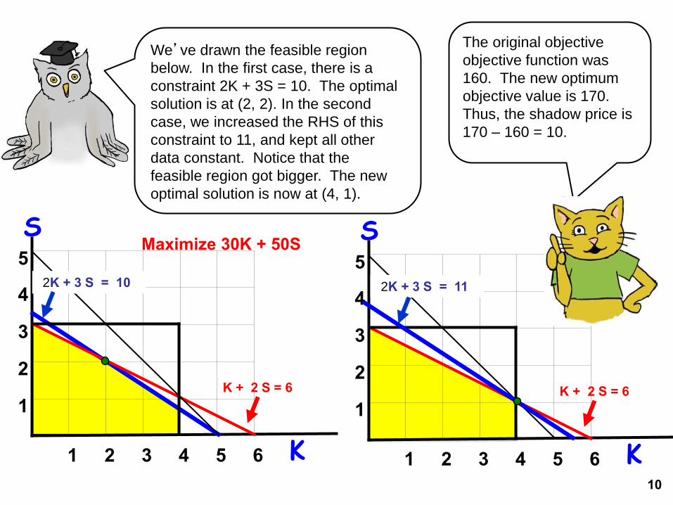
The original objective

objective function was

160. The new optimum

objective value is 170.

Thus, the shadow price is

170 – 160 = 10.

1 2 3 4 5 6

1

2

3

4

5

K

S

K + 2 S = 6

2K + 3 S = 10

1 2 3 4 5 6

1

2

3

4

5

K

S

K + 2 S = 6

2K + 3 S = 11

We’ve drawn the feasible region

below. In the first case, there is a

constraint 2K + 3S = 10. The optimal

solution is at (2, 2). In the second

case, we increased the RHS of this

constraint to 11, and kept all other

data constant. Notice that the

feasible region got bigger. The new

optimal solution is now at (4, 1).

Maximize 30K + 50S

11

1 2 3 4 5 6

1

2

3

4

5

K

S

K + 2 S = 6

2K + 3 S = 10

1 2 3 4 5 6

1

2

3

4

5

K

S

K + 2 S = 6

2K + 3 S = 11

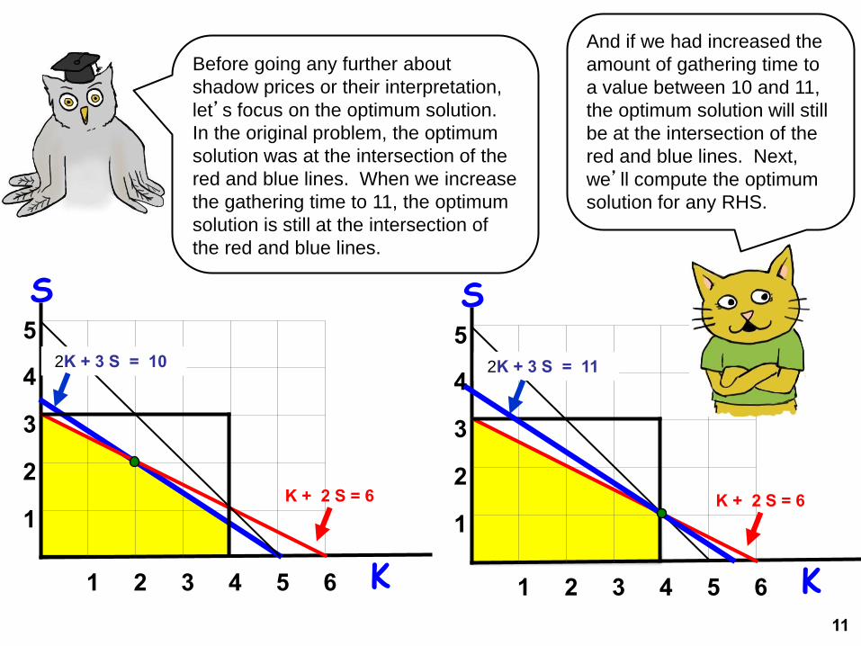
Before going any further about

shadow prices or their interpretation,

let’s focus on the optimum solution.

In the original problem, the optimum

solution was at the intersection of the

red and blue lines. When we increase

the gathering time to 11, the optimum

solution is still at the intersection of

the red and blue lines.

And if we had increased the

amount of gathering time to

a value between 10 and 11,

the optimum solution will still

be at the intersection of the

red and blue lines. Next,

we’ll compute the optimum

solution for any RHS.

12 1 2 3 4 5 6

1

2

3

4

5

K

S

K + 2 S = 6

2K + 3 S = 10 + Δ

Suppose that the amount of

gathering time is changed to 10 +

Δ, where 0 ≤ Δ ≤ 1. The blue line

becomes 2K + 3 S = 10 + Δ.

The red line is K + 2S = 6. The

intersection of the two lines

(expressed as a function of Δ) is

K = 2 + 2Δ; S = 2 – Δ. The

objective value is 30K + 50S =

160 + 10Δ.

Cathy does

those

calculations in

her head.

Wow!

Here is a key point. So long as

0 ≤ Δ ≤ 1, the optimal solution

will be K = 2 + 2Δ; S = 2 – Δ,

and the optimum objective

value will be 160 + 10Δ. If we

let Δ = .6, then the objective

value is 166. Thus, the

increase in the optimum

objective value is 6 = .6 times

the price. Thus the increase in

optimal objective value is

proportional to the increase in

RHS. Δ,

13 1 2 3 4 5 6

1

2

3

4

5

K

S

K + 2 S = 6

2K + 3 S = 10 + Δ

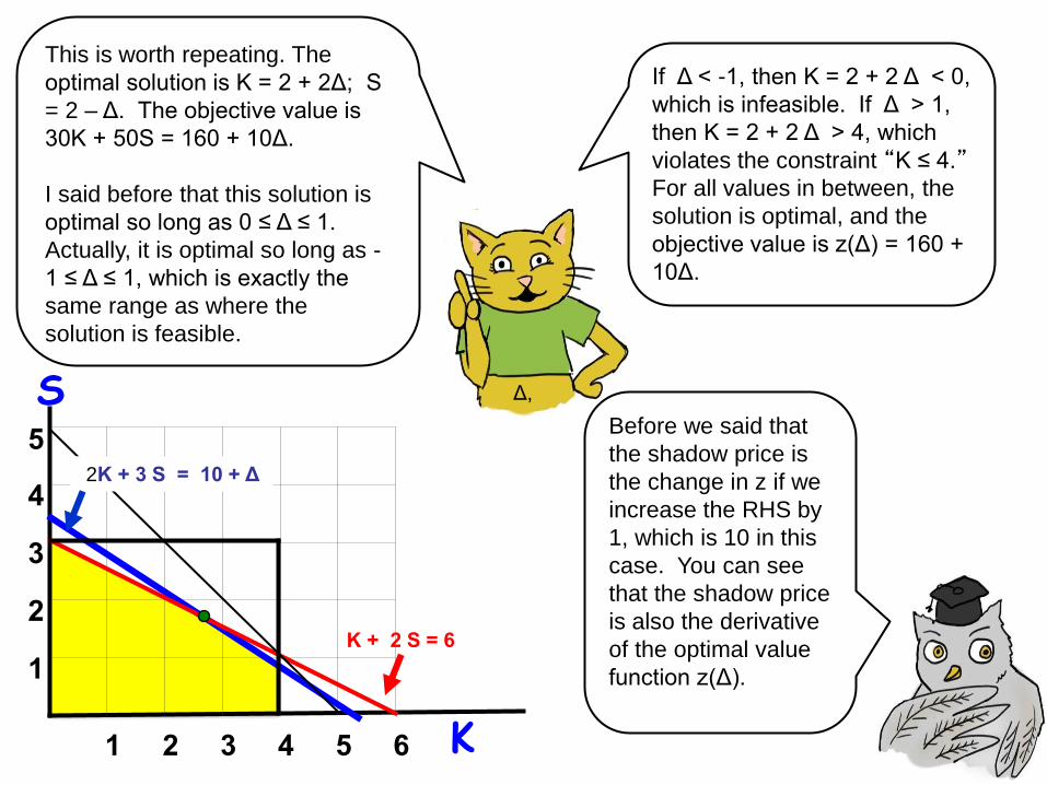
This is worth repeating. The

optimal solution is K = 2 + 2Δ; S

= 2 – Δ. The objective value is

30K + 50S = 160 + 10Δ.

I said before that this solution is

optimal so long as 0 ≤ Δ ≤ 1.

Actually, it is optimal so long as -

1 ≤ Δ ≤ 1, which is exactly the

same range as where the

solution is feasible.

If Δ < -1, then K = 2 + 2 Δ < 0,

which is infeasible. If Δ > 1,

then K = 2 + 2 Δ > 4, which

violates the constraint “K ≤ 4.”

For all values in between, the

solution is optimal, and the

objective value is z(Δ) = 160 +

10Δ.

Δ,

Before we said that

the shadow price is

the change in z if we

increase the RHS by

1, which is 10 in this

case. You can see

that the shadow price

is also the derivative

of the optimal value

function z(Δ).

14

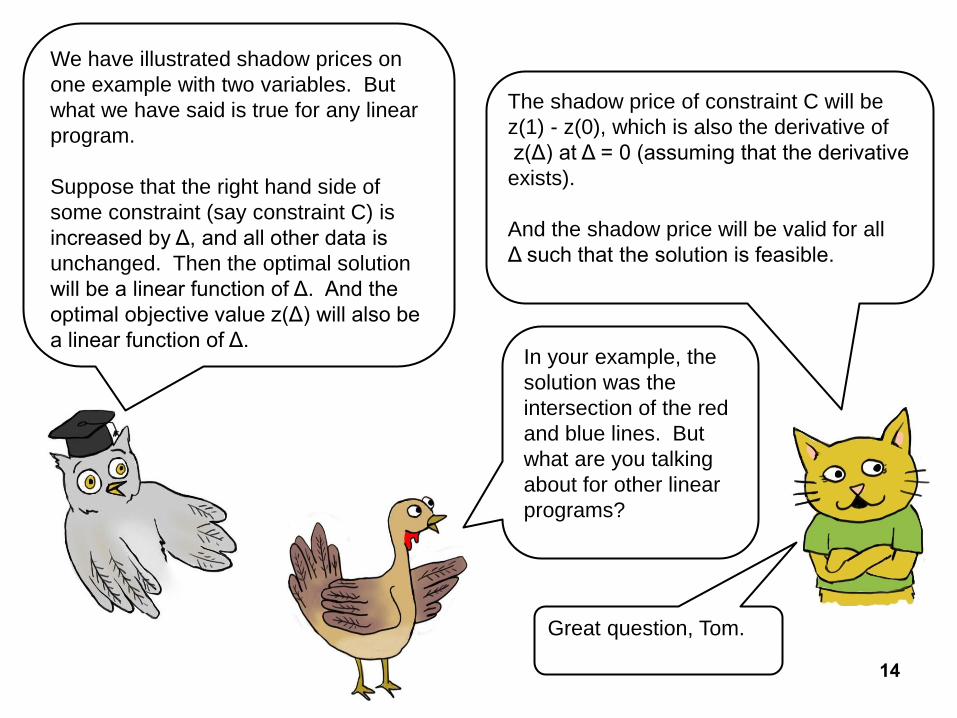
We have illustrated shadow prices on

one example with two variables. But

what we have said is true for any linear

program.

Suppose that the right hand side of

some constraint (say constraint C) is

increased by Δ, and all other data is

unchanged. Then the optimal solution

will be a linear function of Δ. And the

optimal objective value z(Δ) will also be

a linear function of Δ.

The shadow price of constraint C will be

z(1) - z(0), which is also the derivative of

z(Δ) at Δ = 0 (assuming that the derivative

exists).

And the shadow price will be valid for all

Δ such that the solution is feasible.

In your example, the

solution was the

intersection of the red

and blue lines. But

what are you talking

about for other linear

programs?

Great question, Tom.

15

In two dimensional examples (that is,

when there are two variables), the

optimal solution can be described as

the intersection of two lines. As Δ is

increased or decreased from 0, the

optimal solution is still the

intersection of these two lines;

however, now the solution will be a

linear function of Δ.

But you still haven’t

answered my question.

What happens if there are

three or more variables?

Tom, I’ll answer that

question when we

return to the subject

of sensitivity

analysis after

showing how to

solve linear

programs with 3 or

more variables. For

now, I ask you to

have some patience

and trust.

We turkeys are very

trusting and patient.

16

This is a good

time to try it on

your own. Can

you determine

the shadow

price of the

second

constraint?

I’ll get you started.

Consider what happens

when the second

constraint becomes “K +

2S = 6 + Δ”. Then find the

solution to the equations “

“2K + 3S = 10”

“ K + 2S = 6 + Δ”,

and express the solution

as a function of Δ. Also

compute the optimal

objective value z(Δ).

I’ll give you a hint.

The shadow price

is 10.

Nooz, that

isn’t a hint.

That’s the

answer.

But I really want

students to see

how to do the

work. By giving

them the

answer, they

can verify that

they did it

correctly. That’s

pretty foxy.

17

The interval in which the

shadow price is valid is

the interval in which the

solution is feasible. In

this case, the shadow

price is not valid if Δ = 1.

Recall that I first defined the shadow price

of a constraint to be the change in the

optimal objective function if the RHS of the

constraint is increased by 1. Now you can

see why that wasn’t quite precise. This

definition is valid so long as the interval in

which the shadow price is valid contains

“1”. But the definition is close enough to

the truth that it was worth stating.

18

I’m beginning to

understand. But I still

don’t get why we are

doing this. If I want to

find out what happens if

we change part of the

data, it is really easy to

solve a second linear

program.

Tom, I’ll answer that question

when we return to the subject of

sensitivity analysis after showing

how to solve linear programs with

3 or more variables. For now, I

ask you to have some patience

and trust.

I just got a

feeling of déjà

vu.

OK. I’ll try to be

patient.

19

Summary for changes in RHS coefficients • Determine the binding constraints, that is, the constraints that hold with equality.

• Determine the change in the “corner point solution” as a function of Δ.

• Compute the largest and smallest values of Δ so that the solution stays feasible.

• The shadow price is valid so long as the “corner point solution” remains optimal, which is so long as it is feasible.

• If there are three binding constraints, then choose two of these to get the two equations to solve, and the technique still works. (But the shadow prices and ranges depends on which two constraints are chosen.)

And here is a shortcut. Determine the

binding constraints, and determine the

solution to the constraints if the RHS is

increased by 1. (Don’t worry about

feasibility). The shadow price is the increase

in the objective value.

20

We are going to cover one other type of

sensitivity analysis in this tutorial. What is the

effect on the optimum objective function of

changing the cost coefficient of one of the

variables?

Remember that the optimal solution

occurs at a corner point. In this case,

the optimum solution was (2, 2),

which was the intersection of the red

and green line. What do you think

will be the new optimal solution if the

revenue from shields changes just a

little bit?

21

If you answered

that the optimal

solution changes

just a little bit, you

are nearly right.

Ella is being tactful.

Actually, that

answer would be

wrong.

If you answered that the

optimal solution will not

change, then you are

completely right.

But this raises another

question. How much can

you change the cost

coefficient so that the

optimum solution stays the

same?

22

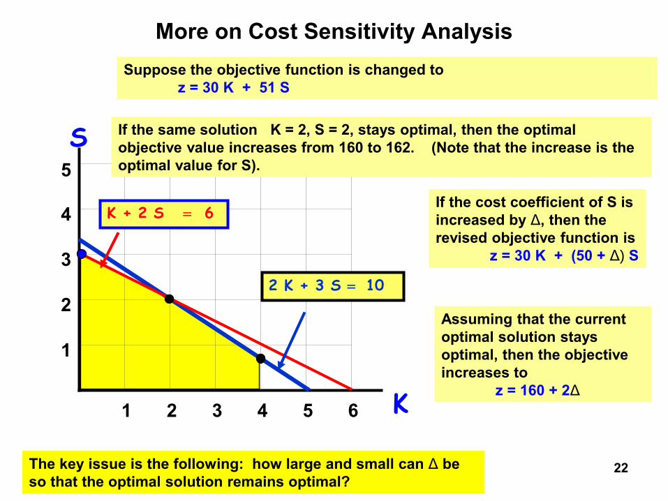
More on Cost Sensitivity Analysis Suppose the objective function is changed to z = 30 K + 51 S

1 2 3 4 5 6

1

2

3

4

5

K

S

2 K + 3 S = 10

K + 2 S = 6

If the same solution K = 2, S = 2, stays optimal, then the optimal objective value increases from 160 to 162. (Note that the increase is the optimal value for S).

If the cost coefficient of S is increased by Δ, then the revised objective function is z = 30 K + (50 + Δ) S

Assuming that the current optimal solution stays optimal, then the objective increases to z = 160 + 2Δ

The key issue is the following: how large and small can Δ be so that the optimal solution remains optimal?

23

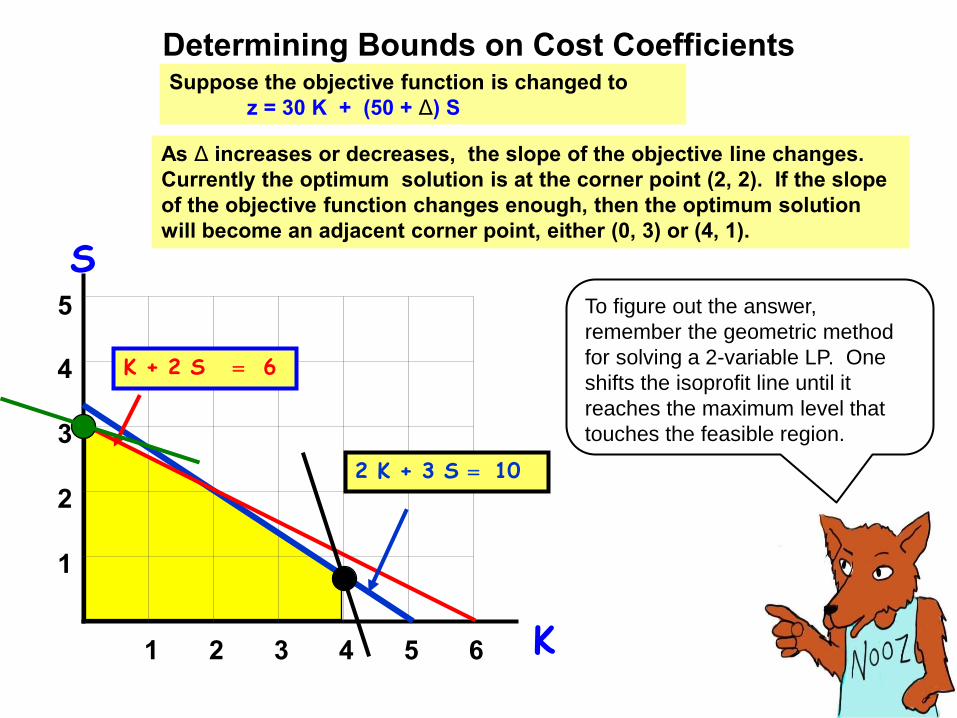
Determining Bounds on Cost Coefficients Suppose the objective function is changed to z = 30 K + (50 + Δ) S

As Δ increases or decreases, the slope of the objective line changes. Currently the optimum solution is at the corner point (2, 2). If the slope of the objective function changes enough, then the optimum solution will become an adjacent corner point, either (0, 3) or (4, 1).

1 2 3 4 5 6

1

2

3

4

5

K

S

2 K + 3 S = 10

K + 2 S = 6

To figure out the answer,

remember the geometric method

for solving a 2-variable LP. One

shifts the isoprofit line until it

reaches the maximum level that

touches the feasible region.

24

Determining Bounds on Cost Coefficients If Δ = -5, the objective is parallel to 2 K + 3 S = 10

So (2, 2) remains optimal if -5 ≤ Δ ≤ 10.

1 2 3 4 5 6

1

2

3

4

5

K

S

2 K + 3 S = 10

K + 2 S = 6

If Δ = 10, the objective is parallel

to ”K + 2 S = 6”. When Δ = 10,

then, every point on the line

segment from (0,3) to (2, 2) is

optimal.

Suppose the objective function is changed to

z = 30 K + (50 + Δ) S

If Δ = 0, the optimal solution is (2, 2). This

solution stays optimal for small positive Δ so

long as Δ < 10.

When Δ = 10, the isoprofit line is

30K + 60S = 180. This is the

same line as K + 2S = 6.

25

Determining Bounds on Cost Coefficients If Δ = -5, the objective is parallel to 2 K + 3 S = 10

So (2, 2) remains optimal if -5 ≤ Δ ≤ 10.

1 2 3 4 5 6

1

2

3

4

5

K

S

2 K + 3 S = 10

K + 2 S = 6

When Δ = -5, the isoprofit line is

30 K + 45 S = 150.

This is the same line as

2K + 3S = 10.

We still assume that the objective function is

z = 30 K + (50 + Δ) S.

If Δ is between 0 and -5, the optimal solution

is (2, 2). If Δ = -5, then, every point on the line

segment from (2, 2) to (4, 1) is optimal.

As Δ changes from -∞ to ∞, each

of the five corner points will be

optimal within a segment.

26

Summary for Changes in the Cost Coefficients Suppose that we want to modify the cost coefficient for a variable xj. We

want to increase it from cj to cj + Δ.

• Determine the binding constraints and the current corner point solution, say x*.

• Compute the largest and smallest values of Δ so that the x* remains optimal. In two dimensions, this will occur when the revised objective function is parallel to one of the constraints.

I really like 2 variable LPs! They are my

favorite LPs, except possibly for LPs with only

one variable.

27

Last Slide

By the way, 2-D LPs are

not so important in and of

themselves. But by

knowing how to do

sensitivity analysis in 2-D,

it’s easier to understand

what happens with

problems with more

variables.

That concludes this tutorial

of sensitivity analysis for

Linear Programming in two

dimensions.

I hope it was helpful. So

long!

MIT OpenCourseWarehttp://ocw.mit.edu

15.053 Optimization Methods in Management ScienceSpring 2013

For information about citing these materials or our Terms of Use, visit: http://ocw.mit.edu/terms.