item response modeling of paired comparison and …item response modeling of paired comparison and...
TRANSCRIPT
Multivariate Behavioral Research, 45:935–974, 2010
Copyright © Taylor & Francis Group, LLC
ISSN: 0027-3171 print/1532-7906 online
DOI: 10.1080/00273171.2010.531231
Item Response Modeling of PairedComparison and Ranking Data
Alberto Maydeu-OlivaresFaculty of Psychology
University of Barcelona
Anna BrownSHL Group
The comparative format used in ranking and paired comparisons tasks can sig-
nificantly reduce the impact of uniform response biases typically associated with
rating scales. Thurstone’s (1927, 1931) model provides a powerful framework for
modeling comparative data such as paired comparisons and rankings. Although
Thurstonian models are generally presented as scaling models, that is, stimuli-
centered models, they can also be used as person-centered models. In this article,
we discuss how Thurstone’s model for comparative data can be formulated as item
response theory models so that respondents’ scores on underlying dimensions can
be estimated. Item parameters and latent trait scores can be readily estimated using
a widely used statistical modeling program. Simulation studies show that item
characteristic curves can be accurately estimated with as few as 200 observations
and that latent trait scores can be recovered to a high precision. Empirical examples
are given to illustrate how the model may be applied in practice and to recommend
guidelines for designing ranking and paired comparisons tasks in the future.
Presenting items in a single-stimulus fashion, using, for instance, rating scales,
often can lead to uniform response biases such as acquiescence and extreme
responding (e.g., Van Herk, Poortinga, & Verhallen, 2004) or lack of differ-
entiation commonly referred to as “halo” effects (Murphy, Jako, & Anhalt,
1993). One approach to overcome this problem is to model such bias (e.g.,
Correspondence concerning this article should be addressed to Alberto Maydeu-Olivares, Faculty
of Psychology, University of Barcelona, P. Valle de Hebrón, 171, 08035, Barcelona, Spain. E-mail:
935
Downloaded By: [Maydeu-Olivares, Albert] At: 17:19 20 December 2010
936 MAYDEU-OLIVARES AND BROWN
Maydeu-Olivares & Coffman, 2006). Another approach is to present test items
instead in a comparative or forced-choice format. This approach can significantly
reduce the impact of numerous uniform response biases (Cheung & Chan,
2002). Thurstone’s (1927, 1931) model provides a powerful framework for
describing the response process to comparative data such as paired comparisons
and rankings. Although Thurstonian models are generally presented as scaling
models, that is, stimuli-centered models, they can also be used as person-centered
models. For instance, in a ranking task, respondents may be presented with a
set of behavioral statements and asked to order them according to the extent
that the statements describe their personality. Or, respondents may be asked
to order a set of attitudinal statements according to the extent they represent
their own attitudes. In a paired comparison task, pairs of statements are selected
from a set of available items, and respondents are instructed to select the item
that best describes them from each pair. In these applications, the focus is
not on the items under comparison and their relationships but rather on the
individuals’ personality traits, attitudes, and so on. When used in this fashion,
Thurstonian models for comparative data are item response theory (IRT) models
(Maydeu-Olivares, 2001). The aim of this article is to describe the properties
and characteristics of Thurstonian models for comparative data as IRT models.
This article is structured into seven sections. In the first section, we describe
how to code rankings and paired comparisons using binary outcome variables.
This binary coding allows straightforward estimation of models for compara-
tive data using standard statistical software. Section two describes Thurstonian
models for comparative data. In this section we provide the response model for
ranking tasks and for paired comparisons tasks. We also describe embedding
common factors in these models. Thurstonian factor models are second-order
normal ogive models with some special features. Section three introduces the
Thurstonian IRT model. This is simply a reparameterization of the Thurstonian
factor model as a first-order model, again with special features. The Thurstonian
IRT model provides some valuable insights into the features of Thurstonian
models as person-centered models and it enables straightforward estimation
of latent trait scores for ranking data, something that is not possible with the
Thurstonian factor model. Section four discusses item parameter estimation of
Thurstonian models for paired comparisons and rankings. Section five provides
a detailed account of the Thurstonian IRT model. In this section we (a) provide
the item characteristic function for these models, (b) discuss how to estimate the
latent traits, and (c) provide the information function and discuss how to estimate
test reliability. Because in today’s IRT applications unidimensional models are
most often used, in this article we focus mostly on unidimensional models.
Section five reports the results of simulation studies to investigate the accuracy
of item parameter estimates and their standard errors, goodness of fit tests, and
latent trait scores. The widely used statistical modeling program Mplus (L. K.
Downloaded By: [Maydeu-Olivares, Albert] At: 17:19 20 December 2010
IRT OF PAIRED COMPARISONS AND RANKINGS 937
Muthén & Muthén, 1998–2009) is used throughout the article to estimate the
item parameters models and to obtain latent trait scores. Section six includes
two applications to illustrate our presentation, one involving ranking data and
one involving paired comparisons data. We conclude with a summary of the
main points of this article and a discussion of extensions of the work presented
here.
BINARY CODING OF COMPARATIVE DATA
This section discusses how to code the observed paired comparison and ranking
data in a form suitable for estimating Thurstonian choice models when using
standard software packages for IRT modeling. This section relies heavily on
Maydeu-Olivares and Böckenholt (2005).
Paired Comparisons
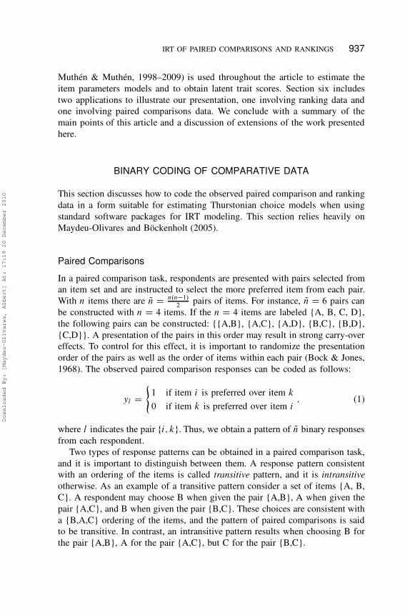
In a paired comparison task, respondents are presented with pairs selected from
an item set and are instructed to select the more preferred item from each pair.
With n items there are Qn D n.n�1/
2pairs of items. For instance, Qn D 6 pairs can
be constructed with n D 4 items. If the n D 4 items are labeled {A, B, C, D},
the following pairs can be constructed: {{A,B}, {A,C}, {A,D}, {B,C}, {B,D},
{C,D}}. A presentation of the pairs in this order may result in strong carry-over
effects. To control for this effect, it is important to randomize the presentation
order of the pairs as well as the order of items within each pair (Bock & Jones,
1968). The observed paired comparison responses can be coded as follows:
yl D(
1 if item i is preferred over item k
0 if item k is preferred over item i; (1)
where l indicates the pair fi; kg. Thus, we obtain a pattern of Qn binary responses
from each respondent.
Two types of response patterns can be obtained in a paired comparison task,
and it is important to distinguish between them. A response pattern consistent
with an ordering of the items is called transitive pattern, and it is intransitive
otherwise. As an example of a transitive pattern consider a set of items {A, B,
C}. A respondent may choose B when given the pair {A,B}, A when given the
pair {A,C}, and B when given the pair {B,C}. These choices are consistent with
a {B,A,C} ordering of the items, and the pattern of paired comparisons is said
to be transitive. In contrast, an intransitive pattern results when choosing B for
the pair {A,B}, A for the pair {A,C}, but C for the pair {B,C}.
Downloaded By: [Maydeu-Olivares, Albert] At: 17:19 20 December 2010
938 MAYDEU-OLIVARES AND BROWN
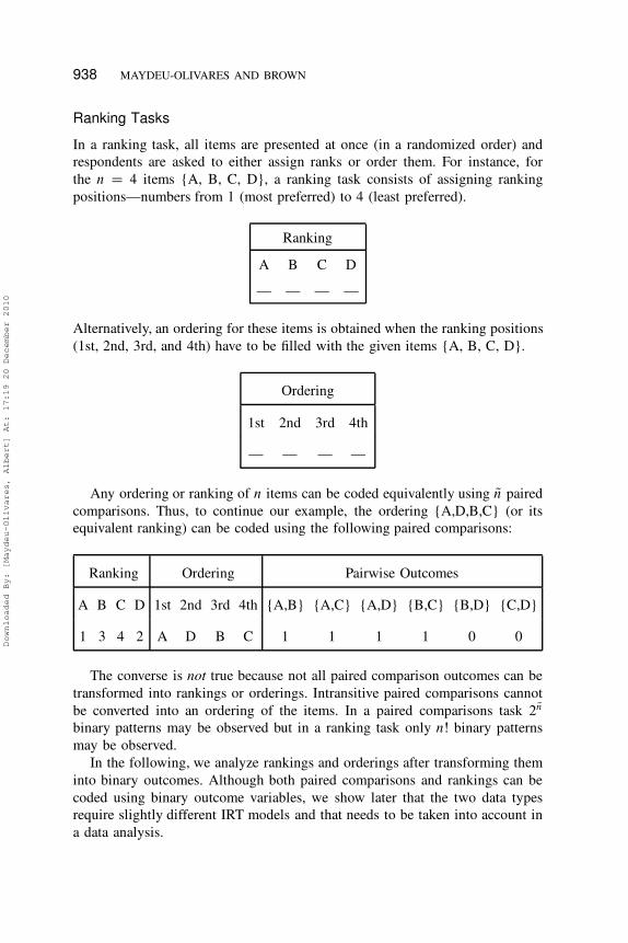
Ranking Tasks
In a ranking task, all items are presented at once (in a randomized order) and
respondents are asked to either assign ranks or order them. For instance, for
the n D 4 items {A, B, C, D}, a ranking task consists of assigning ranking
positions—numbers from 1 (most preferred) to 4 (least preferred).
Ranking
A B C D
— — — —
Alternatively, an ordering for these items is obtained when the ranking positions
(1st, 2nd, 3rd, and 4th) have to be filled with the given items {A, B, C, D}.
Ordering
1st 2nd 3rd 4th
— — — —
Any ordering or ranking of n items can be coded equivalently using Qn paired
comparisons. Thus, to continue our example, the ordering {A,D,B,C} (or its
equivalent ranking) can be coded using the following paired comparisons:
Ranking Ordering Pairwise Outcomes
A B C D 1st 2nd 3rd 4th {A,B} {A,C} {A,D} {B,C} {B,D} {C,D}
1 3 4 2 A D B C 1 1 1 1 0 0
The converse is not true because not all paired comparison outcomes can be
transformed into rankings or orderings. Intransitive paired comparisons cannot
be converted into an ordering of the items. In a paired comparisons task 2Qn
binary patterns may be observed but in a ranking task only nŠ binary patterns
may be observed.
In the following, we analyze rankings and orderings after transforming them
into binary outcomes. Although both paired comparisons and rankings can be
coded using binary outcome variables, we show later that the two data types
require slightly different IRT models and that needs to be taken into account in
a data analysis.
Downloaded By: [Maydeu-Olivares, Albert] At: 17:19 20 December 2010
IRT OF PAIRED COMPARISONS AND RANKINGS 939
THURSTONIAN MODELS FOR RANKING AND PAIRED
COMPARISON DATA
To model comparative data, such as the data arising from a ranking or paired
comparisons task, Thurstone (1927) proposed the so-called Law of Comparative
Judgment. He argued that in a comparative task, (a) each item elicits a utility
as a result of a discriminal process, (b) respondents choose the item with the
largest utility value at the moment of comparison, and (c) the utility is an
unobserved (continuous) variable and is normally distributed in the population
of respondents. Thus, Thurstone’s (1927) approach may be viewed as a latent
variable model where each latent variable corresponds to each of the items
(Maydeu-Olivares, 2002; Takane, 1987). Although he focused initially on paired
comparisons, Thurstone (1931) recognized later that many other types of choice
data, including rankings, could be modeled in a similar way.
Response Model for Ranking Tasks
Consider a random sample of respondents sampled from the population of
interest. According to Thurstone (1927, 1931), when a respondent is confronted
with a ranking task, each of the n items to be ranked elicits a utility. We
denote by ti the utility (a latent variable) associated with item i . Therefore, in
Thurstone’s model there are exactly n such latent variables when modeling n
items. A respondent prefers item i over item k if her or his latent utility for
item i is larger than for item k and consequently ranks item i before item k.
Otherwise, he or she ranks item k before item i . The former outcome is coded
as “1” and the latter as “0.” That is,
yl D(
1 if ti � tk
0 if ti < tk; (2)
where the equality sign is arbitrary as the latent utilities are assumed to be
continuous and thus by definition two latent variables can never take on exactly
the same value.
The response process can be alternatively described by computing differences
between the latent utilities. Let
y�l D ti � tk (3)
be a variable that represents the difference between utilities of items i and k.
Because ti and tk are not observed, y�l
is also unobserved. Then, the relation-
ship between the observed comparative response yl and the latent comparative
Downloaded By: [Maydeu-Olivares, Albert] At: 17:19 20 December 2010
940 MAYDEU-OLIVARES AND BROWN
response y�l is
yl D(
1 if y�l � 0
0 if y�l < 0
: (4)
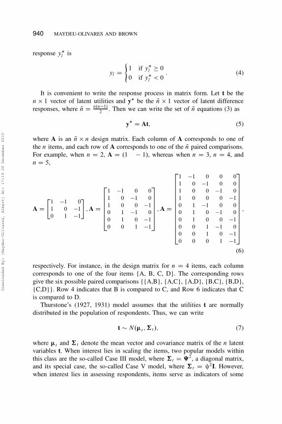
It is convenient to write the response process in matrix form. Let t be the
n � 1 vector of latent utilities and y� be the Qn � 1 vector of latent difference
responses, where Qn D n.n�1/
2. Then we can write the set of Qn equations (3) as
y� D At; (5)
where A is an Qn � n design matrix. Each column of A corresponds to one of
the n items, and each row of A corresponds to one of the Qn paired comparisons.
For example, when n D 2, A D .1 � 1/, whereas when n D 3, n D 4, and
n D 5,
A D"
1 �1 0
1 0 �1
0 1 �1
#
; A D
2
6
6
6
6
6
4
1 �1 0 0
1 0 �1 0
1 0 0 �1
0 1 �1 0
0 1 0 �1
0 0 1 �1
3
7
7
7
7
7
5
; A D
2
6
6
6
6
6
6
6
6
6
6
6
6
4
1 �1 0 0 0
1 0 �1 0 0
1 0 0 �1 0
1 0 0 0 �1
0 1 �1 0 0
0 1 0 �1 0
0 1 0 0 �1
0 0 1 �1 0
0 0 1 0 �1
0 0 0 1 �1
3
7
7
7
7
7
7
7
7
7
7
7
7
5
;
(6)
respectively. For instance, in the design matrix for n D 4 items, each column
corresponds to one of the four items {A, B, C, D}. The corresponding rows
give the six possible paired comparisons {{A,B}, {A,C}, {A,D}, {B,C}, {B,D},
{C,D}}. Row 4 indicates that B is compared to C, and Row 6 indicates that C
is compared to D.
Thurstone’s (1927, 1931) model assumes that the utilities t are normally
distributed in the population of respondents. Thus, we can write
t � N.�t ; †t/; (7)
where �t and †t denote the mean vector and covariance matrix of the n latent
variables t. When interest lies in scaling the items, two popular models within
this class are the so-called Case III model, where †t D ‰2, a diagonal matrix,
and its special case, the so-called Case V model, where †t D §2I. However,
when interest lies in assessing respondents, items serve as indicators of some
Downloaded By: [Maydeu-Olivares, Albert] At: 17:19 20 December 2010
IRT OF PAIRED COMPARISONS AND RANKINGS 941
latent factors (personality traits, motivation factors, attitudes, etc.). Therefore we
need to take an extra step and express the latent variables t as indicators of a
set of m common factors (latent traits):
t D �t C ƒ˜ C ©: (8)
In this equation, �t contains the n means of the latent variables t (i.e., the
utilities’ means), ƒ is an n�m matrix of factor loadings, ˜ is an m-dimensional
vector of common factors (latent traits in IRT terminology), and © is an n-
dimensional vector of unique factors. This factor model assumes that the com-
mon factors have mean zero unit variance and are possibly correlated (their
correlation matrix is ˆ). The model also assumes that the unique factors have
mean zero and are uncorrelated so that their covariance matrix, ‰2, is diago-
nal. In concordance with the distributional assumptions of Thurstonian choice
models, the common and unique factors are assumed to be normally distributed.
Response Model for Paired Comparison Tasks
In a paired comparison task, respondents need not be consistent in their pairwise
choices, possibly yielding intransitive patterns. Inconsistent pairwise responses
can be accounted for by adding an error term el to the difference judgment (3),
y�l D ti � tk C el : (9)
This random error el is assumed to be normally distributed with zero mean and
variance ¨2l, uncorrelated across pairs and uncorrelated with the latent utilities.
The error term accounts for intransitive responses by reversing the sign of the
difference between the utilities ti and tk . For example, suppose that for a given
respondent, ti D 3 and tk D 2. Then, whenever el � 1, y�l � 0 and the
respondent will choose item i over item k. But if el > 1, y�l < 0 and he or she
will choose item k over item i , resulting in an intransitivity because ti > tk .
As in the case of ranking data, the relationship between the observed com-
parative response yl and the latent difference judgment y�l is given by Equation
(4). Similarly, the response process can be written in matrix form as
y� D At C e; (10)
where e is an Qn � 1 vector of random errors with covariance matrix �2, which
is a diagonal matrix with elements ¨21; � � � ; ¨2
Qn.
When the common factor model (8) is embedded in Equation (10) we obtain
y� D A.�t C ƒ˜ C ©/ C e: (11)
Downloaded By: [Maydeu-Olivares, Albert] At: 17:19 20 December 2010
942 MAYDEU-OLIVARES AND BROWN
Also, the mean vector and covariance matrix of the latent differences y� are
�y� D A�t ; and †y� D A.ƒˆƒ0 C ‰2/A0 C �2: (12)
The model for ranking data can be seen as a special case of the model for
paired comparisons. The smaller the diagonal elements of the error covariance
matrix �2, the more consistent the respondents are in evaluating the items. In the
extreme case, when all the diagonal elements of �2 are zero, no intransitivities
would be observed in the data and the paired comparison data are effectively
rankings. A more restricted model that is often found to be useful in applications
involves setting the error variances to be equal for all pairs (i.e., �2 D ¨2I/.
This restriction implies that the number of intransitivities is approximately equal
for all pairs provided the elements of �t are not too dissimilar (Maydeu-Olivares
& Böckenholt, 2005).
Thresholds and Tetrachoric Correlations Implied by
the Model
Because all random variables (˜, ©, and e) are normally distributed, the latent
difference responses y� are also normally distributed. Because the outcome bi-
nary variables y are obtained by dichotomizing the y� variables, the correlations
among the y� variables are tetrachoric correlations.
To obtain the tetrachoric correlations implied by Thurstone’s (1927, 1931)
model we standardize the latent difference responses y� using
z� D D.y� � �y�/; D D .Diag.†y�//� 12 ; (13)
where z� are the standardized latent difference responses and D is a diagonal
matrix with the reciprocals of the model implied standard deviations of y� in the
diagonal. The standardized latent difference responses are multivariate normal
with a 0 mean vector and tetrachoric correlation matrix Pz� , where
Pz� D D.†y�/D: (14)
Using (12), in the special case where a common factor model is assumed to
underlie the utilities, (14) becomes
Pz� D D.†y�/D D D.A.ƒˆƒ0 C ‰2/A0 C �2/D: (15)
The standardized latent difference responses z� are related to the observed
comparative responses y via the threshold relationship
yl D(
1 if z�l � £l
0 if z�l < £l
; (16)
Downloaded By: [Maydeu-Olivares, Albert] At: 17:19 20 December 2010
IRT OF PAIRED COMPARISONS AND RANKINGS 943
where the Qn � 1 vector of thresholds £ has the following structure (Maydeu-
Olivares & Böckenholt, 2005):
£ D �D�y� D �DA�t : (17)
Identification of Thurstonian Factor Models for
Comparative Data
Identification restrictions for these models were given by Maydeu-Olivares and
Böckenholt (2005) and they are the same for ranking and paired comparisons
models. Consider an unrestricted (exploratory) factor model. It is well known
(e.g., McDonald, 1999, p. 181) that this model applied to continuous data can
be identified by setting the factors to be uncorrelated and by setting the upper
triangular part of the factor loading matrix equal to 0. This amounts to setting
œij D 0 for i D 1; : : : ; m � 1; j D i C 1; : : : ; m. For example, with these
constraints the factor loading matrix for a three-factor model has the following
form:
ƒ D
0
B
B
B
B
B
@
œ11 0 0
œ21 œ22 0
œ31 œ32 œ33
::::::
:::
œn1 œn2 œn3
1
C
C
C
C
C
A
: (18)
The resulting solution can then be rotated (orthogonally or obliquely) to obtain
a more interpretable solution.
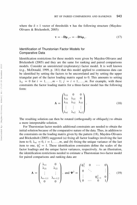
For Thurstonian factor models additional constraints are needed to obtain the
initial solution because of the comparative nature of the data. Thus, in addition to
the constraints on the loading matrix given by the pattern (18), Maydeu-Olivares
and Böckenholt (2005) suggested (a) fixing all factor loadings involving the last
item to 0, œni D 0, i D 1; : : : ; m, and (b) fixing the unique variance of the last
item to one, §2n D 1. These identification constraints define the scales of the
factor loadings and the unique factor variances, respectively. As an illustration,
the identification restrictions needed to estimate a Thurstonian two-factor model
for paired comparisons and ranking data are
ƒ D
0
B
B
B
B
B
@
œ11 0
œ21 œ22
::::::
œn�1;1 œn�1;2
0 0
1
C
C
C
C
C
A
; and ‰2 D
0
B
B
B
B
@
§21 0 � � � 0
0: : :
:::::: §2
n�1 0
0 � � � 0 1
1
C
C
C
C
A
: (19)
Downloaded By: [Maydeu-Olivares, Albert] At: 17:19 20 December 2010
944 MAYDEU-OLIVARES AND BROWN
The necessary identification constraints imply that at least n D 5; 6; 8, and
9 items are required to estimate Thurstonian factor models with m D 1; 2; 3,
and 4 common factors, respectively, in both paired comparisons and ranking
data. Factor models with smaller number of items can also be estimated, but
additional constraints are needed to estimate them.
Regarding the means of the utilities, �t , these parameters can be estimated
by fixing one of the means to some constant, for instance, �n D 0.
Thurstonian Models for Ranking and Paired ComparisonData as IRT Models
In the previous section, we showed that Thurstonian factor models for ranking
and paired comparisons data are indeed a second-order factor model for binary
data with some special features: (a) the number of first-order factors t is fixed by
design; it is n, the number of items; (b) the first-order factor loading matrix, A,
is a matrix of constants—see Equation (6); (c) the uniquenesses of the first-order
factors can be estimated (except for one) because the first-order factor loading
matrix is a matrix of constants; (d) one row of the second-order factor matrix
needs to be fixed to identify the model—see Equation (19); (d) the first-order
factor means may be estimated (these are the mean utilities in Thurstonian
terms); and (e) if the binary outcomes arise from a ranking experiment, the
uniquenesses of the latent response variables must be fixed to zero.
Because factor models for binary data are equivalent to the normal ogive IRT
model (see Takane & de Leeuw, 1987), in this section we exploit this relationship
and present Thurstonian models for comparative data as IRT models. First, we
introduce a Thurstonian factor model with unconstrained thresholds that it is
likely to yield a better fit in applications. Then, we show how the Thurstonian
factor model (which is a second-order model) can be equivalently expressed as
a first-order model with structured correlated errors. We refer to this model as
the Thurstonian IRT model.
Thurstonian Factor Models With Unrestricted Thresholds(Unrestricted Intercepts)
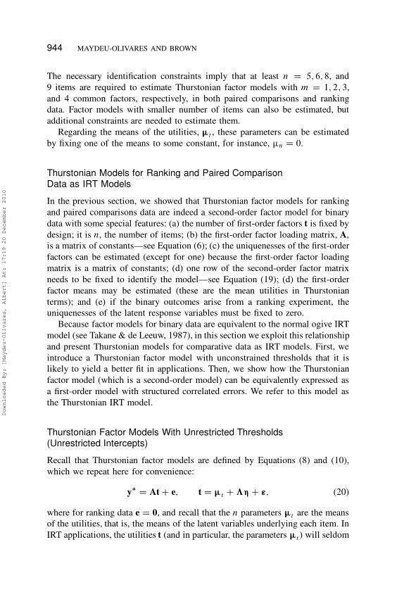
Recall that Thurstonian factor models are defined by Equations (8) and (10),
which we repeat here for convenience:
y� D At C e; t D �t C ƒ˜ C ©; (20)
where for ranking data e D 0, and recall that the n parameters �t are the means
of the utilities, that is, the means of the latent variables underlying each item. In
IRT applications, the utilities t (and in particular, the parameters �t ) will seldom
Downloaded By: [Maydeu-Olivares, Albert] At: 17:19 20 December 2010
IRT OF PAIRED COMPARISONS AND RANKINGS 945
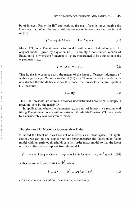
be of interest. Rather, in IRT applications, the main focus is on estimating the
latent traits ˜. When the mean utilities are not of interest, we can use instead
of (20)
y� D �” C At C e; t D ƒ˜ C ©: (21)
Model (21) is a Thurstonian factor model with unrestricted intercepts. The
original model—given by Equation (20)—is simply a constrained version of
Equation (21), where the Qn intercepts �” are constrained to be a function of the
n parameters �t ,
” D �A�t D ��y� : (22)
That is, the intercepts are also the means of the latent difference judgments y�
with a sign change. We refer to Model (21) as a Thurstonian factor model with
unrestricted thresholds because for this model the threshold structure Equation
(17) becomes
£ D D”: (23)
Thus, the threshold structure £ becomes unconstrained because ” is simply a
rescaling of £ by the matrix D.
In applications where the parameters �t are not of interest, we recommend
fitting Thurstonian models with unrestricted thresholds Equation (21) as it leads
to a considerably less constrained model.
Thurstonian IRT Model for Comparative Data
If indeed the latent utilities t are not of interest, as in most typical IRT appli-
cations, we can go one step further and reparameterize the Thurstonian factor
model with unrestricted thresholds as a first-order factor model so that the latent
utilities t effectively disappear from the model:
y� D �” C A.ƒ˜ C ©/ C e D �” C Aƒ˜ C A© C e D �” C Mƒ˜ C M©: (24)
with M© D A© C e, and cov.M©/ D M‰2, where
Mƒ D Aƒ; M‰2 D A‰2A0 C �2; (25)
are an Qn � m matrix and an Qn � Qn matrix, respectively.
Downloaded By: [Maydeu-Olivares, Albert] At: 17:19 20 December 2010
946 MAYDEU-OLIVARES AND BROWN
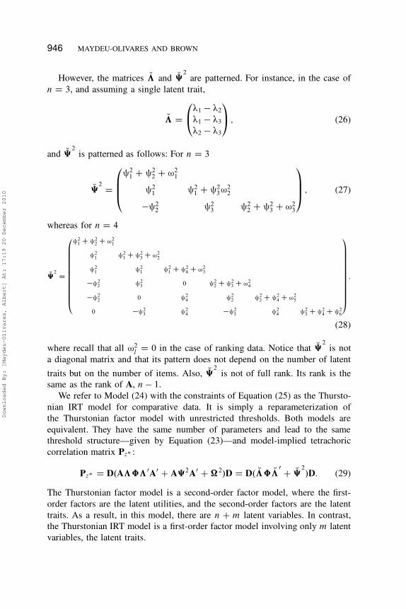
However, the matrices Mƒ and M‰2are patterned. For instance, in the case of
n D 3, and assuming a single latent trait,
Mƒ D
0
@
œ1 � œ2
œ1 � œ3
œ2 � œ3
1
A ; (26)
and M‰2is patterned as follows: For n D 3
M‰2 D
0
B
B
@
§21 C §2
2 C ¨21
§21 §2
1 C §23¨2
2
�§22 §2
3 §22 C §2
3 C ¨23
1
C
C
A
; (27)
whereas for n D 4
M‰2
D
0
B
B
B
B
B
B
B
B
B
B
B
B
@
§2
1C §2
2C ¨2
1
§2
1§2
1C §2
3C ¨2
2
§2
1§2
1§2
1C §2
4C ¨2
3
�§2
2§2
30 §2
2C §2
3C ¨2
4
�§2
20 §2
4§2
2§2
2C §2
4C ¨2
5
0 �§2
3§2
4�§2
3§2
4§2
3C §2
4C §2
6
1
C
C
C
C
C
C
C
C
C
C
C
C
A
;
(28)
where recall that all ¨2l
D 0 in the case of ranking data. Notice that M‰2is not
a diagonal matrix and that its pattern does not depend on the number of latent
traits but on the number of items. Also, M‰2is not of full rank. Its rank is the
same as the rank of A, n � 1.
We refer to Model (24) with the constraints of Equation (25) as the Thursto-
nian IRT model for comparative data. It is simply a reparameterization of
the Thurstonian factor model with unrestricted thresholds. Both models are
equivalent. They have the same number of parameters and lead to the same
threshold structure—given by Equation (23)—and model-implied tetrachoric
correlation matrix Pz� :
Pz� D D.Aƒˆƒ0A0 C A‰2A0 C �2/D D D. Mƒˆ Mƒ0 C M‰2/D: (29)
The Thurstonian factor model is a second-order factor model, where the first-
order factors are the latent utilities, and the second-order factors are the latent
traits. As a result, in this model, there are n C m latent variables. In contrast,
the Thurstonian IRT model is a first-order factor model involving only m latent
variables, the latent traits.
Downloaded By: [Maydeu-Olivares, Albert] At: 17:19 20 December 2010
IRT OF PAIRED COMPARISONS AND RANKINGS 947
Item Parameter Estimation of Thurstonian Models for
Paired Comparisons and Rankings
IRT models are most often estimated using full information maximum likelihood
(FIML—often referred to in the IRT literature as marginal maximum likelihood;
see Bock & Aitkin, 1981). To obtain parameter estimates using FIML, the
probabilities of observing each response pattern are obtained by integrating the
product of the item characteristic curves (ICCs) over the density of the latent
traits, assuming local independence. For the models under consideration, this
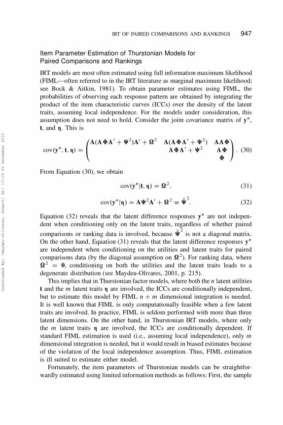
assumption does not need to hold. Consider the joint covariance matrix of y�,
t, and ˜. This is
cov.y�; t; ˜/ D
0
@
A.ƒˆƒ0 C ‰2/A0 C �2 A.ƒˆƒ0 C ‰2/ Aƒˆ
ƒˆƒ0 C ‰2 ƒˆ
ˆ
1
A : (30)
From Equation (30), we obtain
cov.y�jt; ˜/ D �2; (31)
cov.y�j˜/ D A‰2A0 C �2 � M‰2: (32)
Equation (32) reveals that the latent difference responses y� are not indepen-
dent when conditioning only on the latent traits, regardless of whether paired
comparisons or ranking data is involved, because M‰2is not a diagonal matrix.
On the other hand, Equation (31) reveals that the latent difference responses y�
are independent when conditioning on the utilities and latent traits for paired
comparisons data (by the diagonal assumption on �2). For ranking data, where
�2 D 0, conditioning on both the utilities and the latent traits leads to a
degenerate distribution (see Maydeu-Olivares, 2001, p. 215).
This implies that in Thurstonian factor models, where both the n latent utilities
t and the m latent traits ˜ are involved, the ICCs are conditionally independent,
but to estimate this model by FIML n C m dimensional integration is needed.
It is well known that FIML is only computationally feasible when a few latent
traits are involved. In practice, FIML is seldom performed with more than three
latent dimensions. On the other hand, in Thurstonian IRT models, where only
the m latent traits ˜ are involved, the ICCs are conditionally dependent. If
standard FIML estimation is used (i.e., assuming local independence), only m
dimensional integration is needed, but it would result in biased estimates because
of the violation of the local independence assumption. Thus, FIML estimation
is ill suited to estimate either model.
Fortunately, the item parameters of Thurstonian models can be straightfor-
wardly estimated using limited information methods as follows: First, the sample
Downloaded By: [Maydeu-Olivares, Albert] At: 17:19 20 December 2010
948 MAYDEU-OLIVARES AND BROWN
thresholds O£ and the sample tetrachoric correlations O¡ are estimated. Then, the
item parameters of the model are estimated from the first stage estimates by
unweighted least squares (ULS; B. Muthén, 1993) or diagonally weighted least
squares (DWLS; B. Muthén, du Toit, & Spisic, 1997). Limited information
methods and FIML yield very similar IRT parameter estimates and standard
errors (Forero & Maydeu-Olivares, 2009). Also, differences between using ULS
or DWLS in the second stage of the estimation procedure are negligible (Forero,
Maydeu-Olivares, & Gallardo-Pujol, 2009). Furthermore, a test of the restrictions
imposed on the thresholds and tetrachoric correlations is available, with degrees
of freedom equal to the number of thresholds plus the number of tetrachoric
correlations, Qn. QnC1/=2, minus the number of estimated item parameters (say q).
However, care is needed when testing the model with ranking data. This is
because Maydeu-Olivares (1999) showed that when ranking data is used, there
are
r D n.n � 1/.n � 2/=6 (33)
redundancies among the thresholds and tetrachoric correlations estimated from
the binary outcome variables. Hence, the correct number of degrees of freedom
when modeling ranking data is df D Qn. Qn C 1/=2 � r � q. This means that the p
value for the chi-square test statistic needs to be recomputed using the correct
number of degrees of freedom. Also, goodness of fit indices involving degrees
of freedom in their formula, such as the root mean square error of approximation
.RMSEA/ Dq
T �df
df �N, where T denotes the chi-square statistic and N denotes
sample size, also need to be recomputed using the correct degrees of freedom
for ranking data.
THE THURSTONIAN IRT MODEL
In this section, we provide the item characteristic and information function for
the model and discuss item parameter estimation, latent trait estimation, and
reliability estimation. We conclude this section providing some remarks about
the impact of the choice of identification constraints on item parameter estimates.
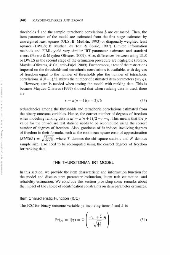
Item Characteristic Function (ICC)
The ICC for binary outcome variable yl involving items i and k is
Pr.yl D 1j˜/ D ˆ
0
B
@
�”l C Mœ0
l˜q
M§2l
1
C
A; (34)
Downloaded By: [Maydeu-Olivares, Albert] At: 17:19 20 December 2010
IRT OF PAIRED COMPARISONS AND RANKINGS 949
where ˆ.x/ denotes a standard normal distribution function evaluated at x, ”l ,
is the threshold for binary outcome yl , Mœ0
l is the 1 � m vector of factor loadings,
and M§2l
is the uniqueness for binary outcome yl .
Equation (34) is simply the ICC of a normal ogive model for binary data
except that (a) Mœ0
l is structured, (b) M§2l is structured, and (c) the ICCs are not
independent (local independence conditional on the latent traits does not hold).
Rather, there are patterned covariances among the unique factors; see Equations
(27) and (28) for the case of three and four items, respectively.
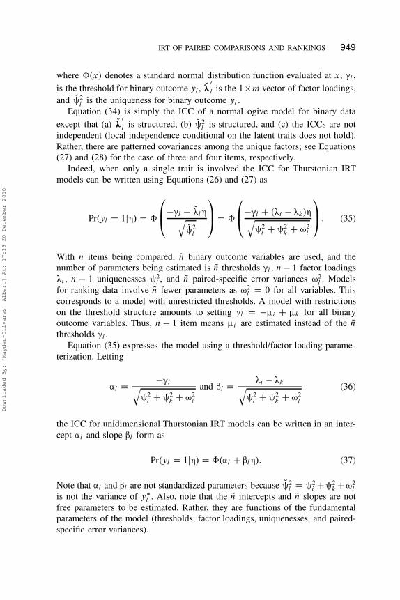
Indeed, when only a single trait is involved the ICC for Thurstonian IRT
models can be written using Equations (26) and (27) as
Pr.yl D 1j˜/ D ˆ
0
B
@
�”l C Mœl ˜q
M§2l
1
C
AD ˆ
0
B
@
�”l C .œi � œk/˜q
§2i C §2
kC ¨2
l
1
C
A: (35)
With n items being compared, Qn binary outcome variables are used, and the
number of parameters being estimated is Qn thresholds ”l , n � 1 factor loadings
œi , n � 1 uniquenesses §2i , and Qn paired-specific error variances ¨2
l . Models
for ranking data involve Qn fewer parameters as ¨2l D 0 for all variables. This
corresponds to a model with unrestricted thresholds. A model with restrictions
on the threshold structure amounts to setting ”l D ��i C �k for all binary
outcome variables. Thus, n � 1 item means �i are estimated instead of the Qnthresholds ”l .
Equation (35) expresses the model using a threshold/factor loading parame-
terization. Letting
’l D �”lq
§2i C §2
kC ¨2
l
and “l D œi � œkq
§2i C §2
kC ¨2
l
(36)
the ICC for unidimensional Thurstonian IRT models can be written in an inter-
cept ’l and slope “l form as
Pr.yl D 1j˜/ D ˆ.’l C “l ˜/: (37)
Note that ’l and “l are not standardized parameters because M§2l D §2
i C§2k C¨2
l
is not the variance of y�l . Also, note that the Qn intercepts and Qn slopes are not
free parameters to be estimated. Rather, they are functions of the fundamental
parameters of the model (thresholds, factor loadings, uniquenesses, and paired-
specific error variances).
Downloaded By: [Maydeu-Olivares, Albert] At: 17:19 20 December 2010
950 MAYDEU-OLIVARES AND BROWN
Latent Trait Estimation, Information Functions, and
Reliability Estimation
After the item parameters have been estimated, latent trait scores can be es-
timated by treating the estimated parameters as if they were known. This is
reasonable if item parameters have been accurately estimated. One approach
to estimate the latent trait scores is by maximum likelihood (ML). Two other
alternative approaches are (a) computing the mean of the posterior distribution
of the latent traits and (b) computing the mode of that distribution. The former is
known as expected a posteriori estimation, and the latter maximum a posteriori
(MAP) estimation (see Bock & Aitkin, 1981). Here, we focus on the MAP
estimator, as it is the method implemented in the software used throughout this
article, Mplus. In passing, we also provide results for the ML estimator.
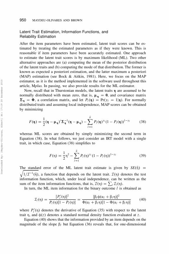
Now, recall that in Thurstonian models, the latent traits ˜ are assumed to be
normally distributed with mean zero, that is, �˜ D 0, and covariance matrix
†˜ D ˆ, a correlation matrix, and let Pl .˜/ D Pr.yl D 1j˜/. For normally
distributed traits and assuming local independence, MAP scores can be obtained
by minimizing
F.˜/ D 1
2.˜ � �˜/0†�1
˜ .˜ � �˜/ �Qn
X
lD1
Pl .˜/yl .1 � Pl .˜//1�yl (38)
whereas ML scores are obtained by simply minimizing the second term in
Equation (38). In what follows, we just consider an IRT model with a single
trait, in which case, Equation (38) simplifies to
F.˜/ D 1
2˜2 �
QnX
lD1
Pl .˜/yl .1 � Pl .˜//1�yl (39)
The standard error of the ML latent trait estimate is given by SE. O / Dq
1=I�1. O/, a function that depends on the latent trait. I.˜/ denotes the test
information function, which, under local independence, can be written as the
sum of the item information functions, that is, I.˜/ DP
l Il.˜/.
In turn, the ML item information for the binary outcome l is obtained as
Il .˜/ D ŒP 0l .˜/�2
Pl .˜/Œ1 � Pl .˜/�D Œ“l¥.’l C “l ˜/�2
ˆ.’l C “l ˜/Œ1 � ˆ.’l C “l ˜/�(40)
where P 0l .˜/ denotes the derivative of Equation (35) with respect to the latent
trait ˜, and ¥.z/ denotes a standard normal density function evaluated at z.
Equation (40) shows that the information provided by an item depends on the
magnitude of the slope “l but Equation (36) reveals that, for one-dimensional
Downloaded By: [Maydeu-Olivares, Albert] At: 17:19 20 December 2010
IRT OF PAIRED COMPARISONS AND RANKINGS 951
models, the slope “l linearly depends on the difference between the factor
loadings œi and œk of the two items involved in the comparison. Also, the
slope “l will be higher the smaller the §2i and ¨2
l parameters. But when factor
loadings œi and œk are similar, the slope “l will be close to zero, and the binary
outcome will not discriminate well among respondents. In applications, unless
items are chosen so that the loadings œi vary widely in their magnitudes, the item
slopes in the one-dimensional Thurstonian IRT model are likely to be low in
applications and a large number of items will be needed to accurately estimate
the latent trait. Equation (36) also reveals that whenever œi < œk , the slope
“l will be negative for one-dimensional models. Thus, in applications negative
estimates for “l will be commonly found. However, it is the magnitude of the
slope parameters “l that matters, not their sign.
Now, the standard error of the MAP latent trait estimate is given by
SE. O / Dq
1=I�1P . O / (41)
where IP .˜/ denotes the test information function of the posterior distribution
of the latent trait. For a single latent trait, which is assumed to be normally
distributed with mean zero and variance 1, the MAP test information function
is
Ip.˜/ D I.˜/ C @2¥.˜/
@˜2D I.˜/ C 1: (42)
In applications, it may be convenient to offer a single index of the precision
of measurement of the latent trait instead of the standard error function Equation
(41), which is a function of the latent trait. Provided the squared standard error
function is relatively uniform, a single index of the precision of measurement
can be obtained using the reliability coefficient (e.g., Bock, 1997)
¡ D ¢2 � ¢2error
¢2: (43)
There are two ways to estimate this coefficient.
One way, referred to as theoretical reliability (du Toit, 2003) involves esti-
mating the average error of measurement as
¢2error
DZ 1
�1
I�1P .˜/¥.˜/d˜; (44)
and using ¢2 D 1 in Equation (43) as this is the assumed value for the variance of
the latent trait. In the case of multiple traits, this procedure becomes unattractive
because it involves integrating a multivariate normal distribution.
Downloaded By: [Maydeu-Olivares, Albert] At: 17:19 20 December 2010
952 MAYDEU-OLIVARES AND BROWN
An alternative way to estimate Equation (43), referred to as empirical relia-
bility, involves estimating ¢2 using the sample variance of the estimated MAP
scores and estimating ¢2error
using the mean of the squared standard errors of the
estimated MAP scores. That is, given a sample of N respondents, and letting
O j be the estimated MAP score for respondent j , we compute
O¢2 D 1
N
X
j
. O j � O/2; O¢2error
D 1
N
X
j
.SE. O j //2 D 1
N
X
j
1
IP . O j /: (45)
In our experience, for long tests, the theoretical and empirical reliabilities are
quite close to each other. In short tests, MAP estimates may shrink toward the
mean, and O¢2 computed using Equation (45) may be low, in which case the
empirical estimate will underestimate the reliability.
In either case, given the estimated reliability, we can estimate the correlation
between the true latent trait and the estimated scores using
corr.˜; O / D p¡: (46)
In closing this subsection, we emphasize that the aforementioned standard
results for unidimensional IRT models do not hold if local independence does not
hold. In particular, when local independence does not hold the test information
cannot be decomposed into the sum of item information functions. Thus, we
shall investigate the extent to which the aforementioned expressions (using the
simplifying assumption that the ICCs of Thurstonian IRT models are locally
independent) provide a sufficiently accurate approximation in applications. Note
that this simplifying assumption is only employed for latent trait estimation, not
for item parameter estimation.
Some Remarks About Parameterizations and the Choiceof Identification Constraints
Here we have followed Maydeu-Olivares and Böckenholt’s (2005) suggestions
regarding the choice of identification constraints, perhaps the most striking of
which is to fix one of the factor loadings to zero. In this subsection we examine
the implications of these identification choices. For ease of exposition, we focus
on a set of items that substantively are assumed to be positively related to a
single latent trait.
Statistically, the choice of identification constraints has no impact whatsoever.
In the previous subsection we have shown that it is the intercepts and slopes (i.e.,
the ICC) that govern item information and consequently latent trait recovery.
Intercepts and slopes are invariant to the choice of identification constraints.
This is shown in Appendix A.
Downloaded By: [Maydeu-Olivares, Albert] At: 17:19 20 December 2010
IRT OF PAIRED COMPARISONS AND RANKINGS 953
Substantively, it is unappealing to fix a factor loading to 0 because it suggests
that one particular item is unrelated to the latent trait. From this point of view, it
may be better to fix one of the loadings to 1 instead or to estimate all loadings
using a sum constraint (e.g.,P
i œi D 1), which would enable computing
standard errors for all loadings. We prefer to fix a factor loading because it is
easier to implement, to remind researchers that there is a constraint among the
loadings, and because using a sum constraint will lead to some factor loadings to
be negative. If one factor loading is fixed to some constant for identification some
factor loading estimates may be negative as well. If item n is fixed for identifi-
cation and a negative factor loading for item i is obtained, this indicates that the
absolute value of œi is smaller than œn. It should not be interpreted as a negative
relationship between item i and the trait. With comparative data, the usual
interpretation of the signs of factor loadings does not hold. This is because when
comparative data is modeled, the scale origin is arbitrary (Böckenholt, 2004), and
there are many sets of thresholds and factor loadings that are consistent with any
given model and a researcher is free to choose the most substantively meaningful
model among the set of equivalent models (Maydeu-Olivares & Hernández,
2007). In fact, one can change the signs of one or more factor loadings to ease
the interpretation of the model according to the substantive theory simply by
changing the identification constraints. The formula presented in Appendix A
can be used to explore the set of thresholds and factor loadings that are equivalent
to those estimated in a given application. The important point is that the chosen
constraints will not alter the binary outcomes’ intercepts and slopes.
SIMULATION STUDIES
It is of interest to know how well the fundamental parameters of the Thurstonian
IRT model (”, œ, §2, and in the case of paired comparisons models, ¨2) can be
estimated. These parameters are difficult to interpret substantively because of the
existence of equivalent models. Thus, it is also of interest to know how well the
intercepts ’ and slopes “ are estimated as these parameters are invariant to the
choice of identification constraints and the ICCs and information function are a
direct function of them. The ’ and “ parameters are obtained as a function of the
parameters ”, œ, §2, and ¨2. Finally, it is also of interest to investigate latent trait
recovery. To address these issues, we performed a number of simulation studies.
Item Parameter Recovery and Goodness of Fit Tests
We considered 12 conditions by crossing three sample sizes (200, 500, and
1,000 respondents), two model sizes (6 and 12 items), and 2 model conditions
(paired comparison models with equal and unequal paired specific variances
Downloaded By: [Maydeu-Olivares, Albert] At: 17:19 20 December 2010
954 MAYDEU-OLIVARES AND BROWN
¨2). One thousand replications were used in each condition. Estimation of the
Thurstonian IRT model was performed via tetrachoric correlations using Mplus.
ULS estimation was used to estimate the fundamental model parameters from
the tetrachoric correlations. The intercepts and slopes were computed in Mplus
from the model parameters and their standard errors obtained using the delta
method.
For 6 items, the true parameters used were œ0 D .1:5; 1; 0; 0; �1; �1:5/,
�0t D .�0:2; 0:2; �:7; :7; 0:2; �0:2/, §20 D .1; � � � ; 1/, ¨20 D .0:3; : : : ; 0:3/. For
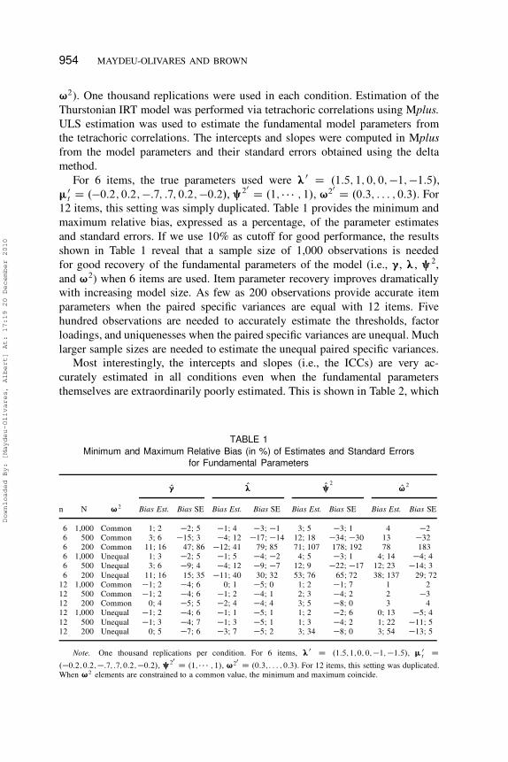
12 items, this setting was simply duplicated. Table 1 provides the minimum and
maximum relative bias, expressed as a percentage, of the parameter estimates
and standard errors. If we use 10% as cutoff for good performance, the results
shown in Table 1 reveal that a sample size of 1,000 observations is needed
for good recovery of the fundamental parameters of the model (i.e., ”, œ, §2,
and ¨2) when 6 items are used. Item parameter recovery improves dramatically
with increasing model size. As few as 200 observations provide accurate item
parameters when the paired specific variances are equal with 12 items. Five
hundred observations are needed to accurately estimate the thresholds, factor
loadings, and uniquenesses when the paired specific variances are unequal. Much
larger sample sizes are needed to estimate the unequal paired specific variances.
Most interestingly, the intercepts and slopes (i.e., the ICCs) are very ac-
curately estimated in all conditions even when the fundamental parameters
themselves are extraordinarily poorly estimated. This is shown in Table 2, which
TABLE 1
Minimum and Maximum Relative Bias (in %) of Estimates and Standard Errors
for Fundamental Parameters
O” Oœ O§2
O2
n N ¨2Bias Est. Bias SE Bias Est. Bias SE Bias Est. Bias SE Bias Est. Bias SE
6 1,000 Common 1; 2 �2; 5 �1; 4 �3; �1 3; 5 �3; 1 4 �2
6 500 Common 3; 6 �15; 3 �4; 12 �17; �14 12; 18 �34; �30 13 �32
6 200 Common 11; 16 47; 86 �12; 41 79; 85 71; 107 178; 192 78 183
6 1,000 Unequal 1; 3 �2; 5 �1; 5 �4; �2 4; 5 �3; 1 4; 14 �4; 4
6 500 Unequal 3; 6 �9; 4 �4; 12 �9; �7 12; 9 �22; �17 12; 23 �14; 3
6 200 Unequal 11; 16 15; 35 �11; 40 30; 32 53; 76 65; 72 38; 137 29; 72
12 1,000 Common �1; 2 �4; 6 0; 1 �5; 0 1; 2 �1; 7 1 2
12 500 Common �1; 2 �4; 6 �1; 2 �4; 1 2; 3 �4; 2 2 �3
12 200 Common 0; 4 �5; 5 �2; 4 �4; 4 3; 5 �8; 0 3 4
12 1,000 Unequal �1; 2 �4; 6 �1; 1 �5; 1 1; 2 �2; 6 0; 13 �5; 4
12 500 Unequal �1; 3 �4; 7 �1; 3 �5; 1 1; 3 �4; 2 1; 22 �11; 5
12 200 Unequal 0; 5 �7; 6 �3; 7 �5; 2 3; 34 �8; 0 3; 54 �13; 5
Note. One thousand replications per condition. For 6 items, œ0D .1:5; 1; 0; 0;�1; �1:5/, �0
tD
.�0:2; 0:2;�:7; :7; 0:2;�0:2/, §20
D .1; � � � ; 1/, ¨20
D .0:3; : : : ; 0:3/. For 12 items, this setting was duplicated.
When ¨2 elements are constrained to a common value, the minimum and maximum coincide.
Downloaded By: [Maydeu-Olivares, Albert] At: 17:19 20 December 2010
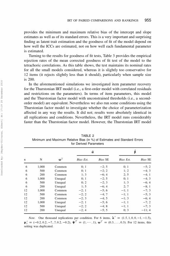
IRT OF PAIRED COMPARISONS AND RANKINGS 955
provides the minimum and maximum relative bias of the intercept and slope
estimates as well as of its standard errors. This is a very important and surprising
finding as latent trait estimation and the goodness of fit of the model depend on
how well the ICCs are estimated, not on how well each fundamental parameter
is estimated.
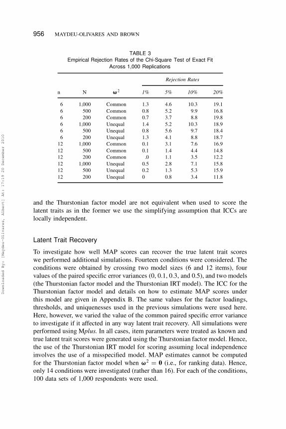
Turning to the results for goodness of fit tests, Table 3 provides the empirical
rejection rates of the mean corrected goodness of fit test of the model to the
tetrachoric correlations. As this table shows, the test maintains its nominal rates
for all the small models considered, whereas it is slightly too conservative for
12 items (it rejects slightly less than it should), particularly when sample size
is 200.
In the aforementioned simulations we investigated item parameter recovery
for the Thurstonian IRT model (i.e., a first-order model with correlated residuals
and restrictions on the parameters). In terms of item parameters, this model
and the Thurstonian factor model with unconstrained thresholds (i.e., a second-
order model) are equivalent. Nevertheless we also run some conditions using the
Thurstonian factor model to investigate whether the choice of parameterization
affected in any way the results. It did not; results were absolutely identical in
all replications and conditions. Nevertheless, the IRT model runs considerably
faster than the Thurstonian factor model. However, the Thurstonian IRT model
TABLE 2
Minimum and Maximum Relative Bias (in %) of Estimates and Standard Errors
for Derived Parameters
O’ O“
n N ¨2 Bias Est. Bias SE Bias Est. Bias SE
6 1,000 Common 0; 1 �2; 5 0; 1 �5; 2
6 500 Common 0; 1 �2; 2 1; 2 �4; 3
6 200 Common 1; 3 �6; 4 2; 5 �4; 1
6 1,000 Unequal 0; 1 �2; 5 0; 1 �4; 3
6 500 Unequal 0; 2 �2; 3 1; 3 �6; 4
6 200 Unequal 1; 5 �6; 4 2; 7 �8; 1
12 1,000 Common �2; 1 �5; 6 �1; 1 �7; 3
12 500 Common �2; 2 �4; 7 �1; 1 �5; 3
12 200 Common �2; 3 �4; 5 �1; 3 �6; 4
12 1,000 Unequal �2; 1 �5; 6 �1; 1 �7; 2
12 500 Unequal �2; 2 �4; 8 �1; 1 �7; 3
12 200 Unequal �2; 4 �5; 5 0; 3 �11; 4
Note. One thousand replications per condition. For 6 items, œ0 D .1:5; 1; 0; 0; �1; �1:5/,
�0
t D .�0:2; 0:2; �7; :7; 0:2; �0:2/, §20
D .1; � � � ; 1/, ¨20
D .0:3; : : : ; 0:3/. For 12 items, this
setting was duplicated.
Downloaded By: [Maydeu-Olivares, Albert] At: 17:19 20 December 2010
956 MAYDEU-OLIVARES AND BROWN
TABLE 3
Empirical Rejection Rates of the Chi-Square Test of Exact Fit
Across 1,000 Replications
Rejection Rates
n N ¨2 1% 5% 10% 20%
6 1,000 Common 1.3 4.6 10.3 19.1
6 500 Common 0.8 5.2 9.9 16.8
6 200 Common 0.7 3.7 8.8 19.8
6 1,000 Unequal 1.4 5.2 10.3 18.9
6 500 Unequal 0.8 5.6 9.7 18.4
6 200 Unequal 1.3 4.1 8.8 18.7
12 1,000 Common 0.1 3.1 7.6 16.9
12 500 Common 0.1 1.4 4.4 14.8
12 200 Common .0 1.1 3.5 12.2
12 1,000 Unequal 0.5 2.8 7.1 15.8
12 500 Unequal 0.2 1.3 5.3 15.9
12 200 Unequal 0 0.8 3.4 11.8
and the Thurstonian factor model are not equivalent when used to score the
latent traits as in the former we use the simplifying assumption that ICCs are
locally independent.
Latent Trait Recovery
To investigate how well MAP scores can recover the true latent trait scores
we performed additional simulations. Fourteen conditions were considered. The
conditions were obtained by crossing two model sizes (6 and 12 items), four
values of the paired specific error variances (0, 0.1, 0.3, and 0.5), and two models
(the Thurstonian factor model and the Thurstonian IRT model). The ICC for the
Thurstonian factor model and details on how to estimate MAP scores under
this model are given in Appendix B. The same values for the factor loadings,
thresholds, and uniquenesses used in the previous simulations were used here.
Here, however, we varied the value of the common paired specific error variance
to investigate if it affected in any way latent trait recovery. All simulations were
performed using Mplus. In all cases, item parameters were treated as known and
true latent trait scores were generated using the Thurstonian factor model. Hence,
the use of the Thurstonian IRT model for scoring assuming local independence
involves the use of a misspecified model. MAP estimates cannot be computed
for the Thurstonian factor model when ¨2 D 0 (i.e., for ranking data). Hence,
only 14 conditions were investigated (rather than 16). For each of the conditions,
100 data sets of 1,000 respondents were used.
Downloaded By: [Maydeu-Olivares, Albert] At: 17:19 20 December 2010
IRT OF PAIRED COMPARISONS AND RANKINGS 957
TABLE 4
Average Correlations Between True Latent Trait Scores and MAP Scores
Across 100 Sets of 1,000 Respondents
Correlations Between
Items ¨2
True Scores
and MAP
Scores
True Scores and MAP
Scores Assuming Local
Independence
MAP Scores and MAP Scores
Assuming Local
Independence
6 0 — 0.873 —
6 0.1 0.872 0.871 0.997
6 0.3 0.871 0.870 0.998
6 0.5 0.871 0.869 0.998
12 0 — 0.936 —
12 0.1 0.937 0.935 0.997
12 0.3 0.936 0.932 0.997
12 0.5 0.934 0.928 0.997
Note. MAP D maximum a posteriori. Item parameters are assumed to be known. For 6 items,
œ0 D .1:5; 1; 0; 0; �1; �1:5/, �0
t D .�0:2; 0:2; �:7; :7; 0:2; �0:2/, §20
D .1, � � � , 1/. For 12 items,
this setting was duplicated. ¨2 D 0 implies ranking data; in this case MAP scores cannot be
computed easily without assuming local independence.
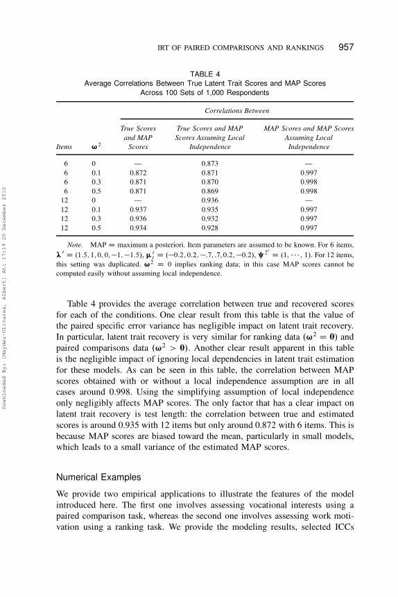
Table 4 provides the average correlation between true and recovered scores
for each of the conditions. One clear result from this table is that the value of
the paired specific error variance has negligible impact on latent trait recovery.
In particular, latent trait recovery is very similar for ranking data .¨2 D 0/ and
paired comparisons data .¨2 > 0/. Another clear result apparent in this table
is the negligible impact of ignoring local dependencies in latent trait estimation
for these models. As can be seen in this table, the correlation between MAP
scores obtained with or without a local independence assumption are in all
cases around 0.998. Using the simplifying assumption of local independence
only negligibly affects MAP scores. The only factor that has a clear impact on
latent trait recovery is test length: the correlation between true and estimated
scores is around 0.935 with 12 items but only around 0.872 with 6 items. This is
because MAP scores are biased toward the mean, particularly in small models,
which leads to a small variance of the estimated MAP scores.
Numerical Examples
We provide two empirical applications to illustrate the features of the model
introduced here. The first one involves assessing vocational interests using a
paired comparison task, whereas the second one involves assessing work moti-
vation using a ranking task. We provide the modeling results, selected ICCs
Downloaded By: [Maydeu-Olivares, Albert] At: 17:19 20 December 2010
958 MAYDEU-OLIVARES AND BROWN
and information functions, and estimations of true score recovery for these
applications.
Example 1: Modeling vocational interests using a paired comparisons
task. Elosua (2007) collected data from 1,069 adolescents in the Spanish
Basque Country using the 16PF Adolescent Personality Questionnaire (APQ;
Schuerger, 2001). The Work Activity Preferences section of this questionnaire
includes a paired comparisons task involving the six types of Holland’s RIASEC
model (see Holland, 1997): Realistic, Investigative, Artistic, Social, Enterprising,
and Conventional. For each of the 15 pairs, respondents were asked to choose
their future preferred work activity. Typically, one would be interested in the
actual utilities of vocational interests in this paired comparison task (first-order
latent variables), but other higher order vocational factors might also be of
interest. Factorial representations of the RIASEC model have been extensively
researched and discussed in the literature. Rounds and Tracey (1993) examined
77 published RIASEC correlation matrices and concluded that, taken together,
these studies suggested the presence of a general factor with equal loadings
on all specific interests, which they interpreted as bias. However, this uniform
biasing factor would not be observed here due to the comparative nature of
the task (Cheung & Chan, 2002). The remaining variance, Rounds and Tracey
(1993) suggested, is best explained by the original theory-based circumplex.
In Hogan’s (1983) interpretation, for instance, one of the two orthogonal axes
on the circumplex was Conformity, with Conventional at the positive pole and
Artistic at the negative pole, Enterprising and Realistic loading positively, and
Social and Investigative negatively. For the purposes of illustration we will fit
a unidimensional Thurstonian IRT model here with the latent trait representing
Conformity.
Thus, we fitted a one-dimensional model with unrestricted thresholds. The
model yields a chi-square of 102.427 on 80 df, p D :046, RMSEA D 0.016.
The model fits rather well. Next, we consider obtaining a more parsimonious
model. One way to do this is to set all the variances of the paired comparison
specific errors ¨2l equal. In so doing, we obtain a chi-square of 155.940 on 94
df, RMSEA D 0.025. Clearly, this model fits more poorly, suggesting that the
number of intransitivities may not be approximately equal across pairs. Another
way to obtain a more parsimonious model is to constrain the thresholds ”l
by estimating the mean utilities �i . In this case, we obtain a chi-square of
150.873 on 90 df, RMSEA D 0.025. Therefore, this model also fits more poorly
that our initial model. The best fitting unidimensional model for these data is
the unrestricted one-dimensional model. We provide in Table 5 the parameter
estimates and standard errors for this model.
It can be seen that an arbitrary choice of identification constraints in this case
yielded a set of parameters that match well with the substantive theory. In line
Downloaded By: [Maydeu-Olivares, Albert] At: 17:19 20 December 2010
IRT OF PAIRED COMPARISONS AND RANKINGS 959
TABLE 5
One-Dimensional Thurstonian IRT Model for Paired Comparisons Data,
Vocational Interests Example, Parameter Estimates, and Standard Errors
l D i,j ”l ¨2
li œi §2
i
1,2 0.742 (0.093) 1.003 (0.302) 1 �0.026 (0.089) 1.692 (0.226)
1,3 0.421 (0.081) 1.146 (0.296) 2 �0.284 (0.083) 0.892 (0.132)
1,4 0.055 (0.063) 0.464 (0.189) 3 �0.898 (0.143) 0.464 (0.154)
1,5 0.807 (0.103) 1.213 (0.358) 4 0.511 (0.120) 0.224 (0.178)
1,6 �0.035 (0.067) 0.346 (0.193) 5 �0.636 (0.106) 1.534 (0.253)
2,3 �0.35 (0.068) 0.778 (0.233) 6 0 (fixed) 1 (fixed)
2,4 �0.644 (0.084) 0.831 (0.256)
2,5 0.172 (0.07) 0.572 (0.252)
2,6 �0.858 (0.084) 0.505 (0.215)
3,4 �0.517 (0.079) 0.639 (0.219)
3,5 0.329 (0.067) 0.521 (0.222)
3,6 �0.48 (0.072) 0.639 (0.209)
4,5 0.768 (0.106) 1.799 (0.444)
4,6 0.079 (0.07) 1.815 (0.483)
5,6 �1.45 (0.14) 2.523 (0.560)
Note. IRT D item response theory. Standard errors in parentheses. The items are 1 D Realistic,
2 D Investigative, 3 D Artistic, 4 D Conventional, 5 D Social, 6 D Enterprising.
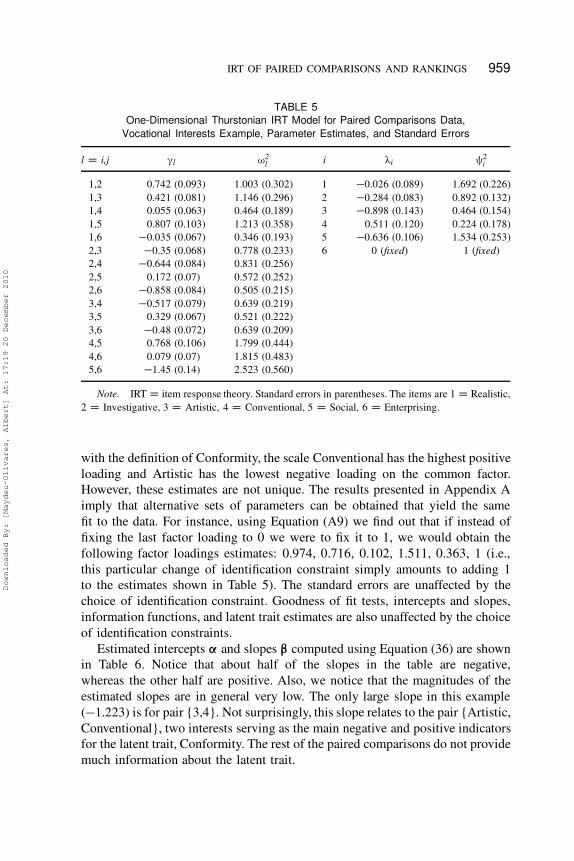
with the definition of Conformity, the scale Conventional has the highest positive
loading and Artistic has the lowest negative loading on the common factor.
However, these estimates are not unique. The results presented in Appendix A
imply that alternative sets of parameters can be obtained that yield the same
fit to the data. For instance, using Equation (A9) we find out that if instead of
fixing the last factor loading to 0 we were to fix it to 1, we would obtain the
following factor loadings estimates: 0.974, 0.716, 0.102, 1.511, 0.363, 1 (i.e.,
this particular change of identification constraint simply amounts to adding 1
to the estimates shown in Table 5). The standard errors are unaffected by the
choice of identification constraint. Goodness of fit tests, intercepts and slopes,
information functions, and latent trait estimates are also unaffected by the choice
of identification constraints.
Estimated intercepts ’ and slopes “ computed using Equation (36) are shown
in Table 6. Notice that about half of the slopes in the table are negative,
whereas the other half are positive. Also, we notice that the magnitudes of the
estimated slopes are in general very low. The only large slope in this example
(�1.223) is for pair {3,4}. Not surprisingly, this slope relates to the pair {Artistic,
Conventional}, two interests serving as the main negative and positive indicators
for the latent trait, Conformity. The rest of the paired comparisons do not provide
much information about the latent trait.
Downloaded By: [Maydeu-Olivares, Albert] At: 17:19 20 December 2010
960 MAYDEU-OLIVARES AND BROWN
TABLE 6
Intercepts and Slopes for the Vocational Interests
Example, Parameter Estimates, and Standard Errors
l D i,k ’l “l
1,2 �0.392 (0.057) 0.136 (0.047)
1,3 �0.232 (0.048) 0.480 (0.079)
1,4 �0.036 (0.041) �0.347 (0.092)
1,5 �0.383 (0.056) 0.290 (0.051)
1,6 0.020 (0.038) �0.015 (0.051)
2,3 0.240 (0.052) 0.421 (0.090)
2,4 0.461 (0.078) �0.569 (0.112)
2,5 �0.099 (0.041) 0.204 (0.054)
2,6 0.554 (0.063) �0.184 (0.053)
3,4 0.448 (0.087) �1.223 (0.152)
3,5 �0.207 (0.046) �0.165 (0.079)
3,6 0.331 (0.055) �0.620 (0.107)
4,5 �0.407 (0.068) 0.608 (0.084)
4,6 �0.045 (0.040) 0.293 (0.081)
5,6 0.645 (0.077) �0.284 (0.047)
Note. The items are 1 D Realistic, 2 D Investigative,
3 D Artistic, 4 D Conventional, 5 D Social, 6 D Enterprising.
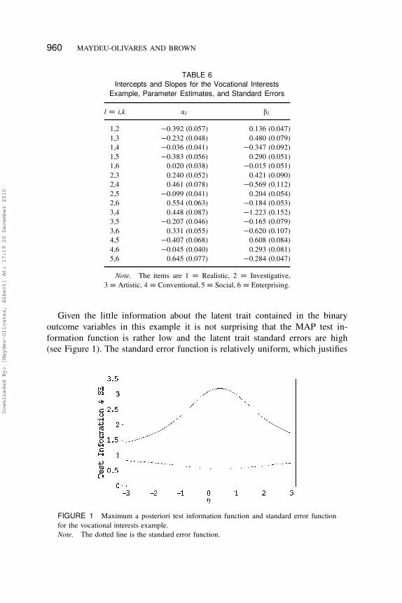
Given the little information about the latent trait contained in the binary
outcome variables in this example it is not surprising that the MAP test in-
formation function is rather low and the latent trait standard errors are high
(see Figure 1). The standard error function is relatively uniform, which justifies
FIGURE 1 Maximum a posteriori test information function and standard error function
for the vocational interests example.
Note. The dotted line is the standard error function.
Downloaded By: [Maydeu-Olivares, Albert] At: 17:19 20 December 2010
IRT OF PAIRED COMPARISONS AND RANKINGS 961
computing a single reliability index to summarize the precision of measure-
ment across the latent trait continuum. Using Equation (44), the estimated
average error of estimation of MAP scores is 0.38, which yields a theoretical
estimate of reliability of 1 � 0:38 D 0:62. The empirical estimated average
error of estimation, computed using Equation (45), is 0.36, quite close to the
theoretical estimate. However, the MAP estimates in this application are quite
shrunken toward the mean and the sample variance of the estimated MAP
scores, computed using Equation (45), is only 0.64, which leads to a very low
empirical estimate of reliability, 0.43. Thus, in this application the empirical
estimate of reliability underestimates quite markedly the theoretical reliability.
In either case, we conclude that although the model appears to fit well, the
precision of measurement obtained is unacceptable. However, this particular
paired comparisons task was used as an illustration as it was not designed
to measure a single underlying trait. Instead, the parameters of the utilities
(vocational interests) would be of interest here.
Example 2: Modeling work motivation using a ranking task. This em-
pirical example is based on ranking data collected as part of a research in
the area of work motivation (Yang, Inceoglu, & Silvester, 2010). Nine broad
features of the work environment that are positively related to employee well-
being, for example “personal development,” were developed from ideas found in
the literature on person-environment fit and the vitamin model of Warr (2007).
1. Supportive Environment.
2. Challenging Work.
3. Career Progression.
4. Ethics.
5. Personal Impact.
6. Personal Development.
7. Social Interaction.
8. Competition.
9. Work Security.
A hypothesized common factor underlying these generally desirable work fea-
tures is general work motivation, that is, having strong drive for working and
achieving. One thousand eighty volunteers were asked to rank these job features
“according to how important it is for you to have these in your ideal job.”
Extended descriptions of the job features were presented to the participants, for
example, “The opportunity to develop your knowledge and skills and to get
feedback on what you do well and less well.”
After transforming the observed ranks into binary outcomes, we fitted a
unidimensional Thurstonian IRT model. Using DWLS estimation Mplus yielded
Downloaded By: [Maydeu-Olivares, Albert] At: 17:19 20 December 2010

962 MAYDEU-OLIVARES AND BROWN
a mean corrected chi-square of 3121.126 on 614 df, RMSEA D 0.062. However,
because the binary outcomes arise from rankings the degrees of freedom (and
the RMSEA) need to be adjusted using Equation (33). The correct number
of degrees of freedom is 594 but the RMSEA is still 0.062. The model fits
acceptably. Table 7 displays the estimated factor loadings and uniquenesses. As
we can see in this table, the job characteristic that is more strongly related to
general work motivation is having a challenging work environment followed by
career progression and supportive environment. Interestingly, the characteristic
that is least strongly related to work motivation is having work security.
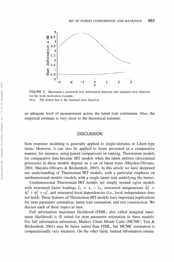
Figure 2 shows the MAP information function (and the SE function) for this
example. Interestingly, individuals scoring low on work motivation are measured
with higher precision than individuals high on work motivation. Also, we ob-
tain smaller standard errors in this application than in the vocational interest
application (there are more binary outcomes in this application). The standard
error function is not too uniform, but we compute the reliability estimate for
this example. Using Equation (44), the estimated average error of MAP scores is
0.26. Thus, the theoretical estimate of reliability is 0.74. The empirical estimated
average error of estimation, computed using Equation (45), is 0.27, quite close to
the theoretical estimate, and the sample variance of the estimated MAP scores,
computed using Equation (45), is 1.09, which leads to an empirical estimate of
reliability of 0.76. Thus, in this application both estimates of reliability suggest
TABLE 7
One-Dimensional Thurstonian IRT Model for Ranking
Data, Work Motivation Example, Factor Loading, and
Uniqueness Estimates and Their Standard Errors
i œi §2
i
1 1.028 (0.158) 1.330 (0.222)
2 1.313 (0.157) 0.851 (0.167)
3 1.104 (0.154) 1.123 (0.193)
4 0.931 (0.145) 0.998 (0.164)
5 0.882 (0.136) 0.878 (0.144)
6 0.908 (0.143) 0.566 (0.092)
7 0.539 (0.122) 0.613 (0.108)
8 0.330 (0.120) 10.346 (0.249)
9 0 (fixed) 1 (fixed)
Note. Standard errors in parentheses. The thresholds are
not shown. The paired specific errors are fixed to zero. The
items are 1 D Supportive Environment, 2 D Challenging
Work, 3 D Career Progression, 4 D Ethics, 5 D Personal
Impact, 6 D Personal Development, 7 D Social Interaction,
8 D Competition, 9 D Work Security.
Downloaded By: [Maydeu-Olivares, Albert] At: 17:19 20 December 2010
IRT OF PAIRED COMPARISONS AND RANKINGS 963
FIGURE 2 Maximum a posteriori test information function and standard error function
for the work motivation example.
Note. The dotted line is the standard error function.
an adequate level of measurement across the latent trait continuum. Also, the
empirical estimate is very close to the theoretical estimate.
DISCUSSION
Item response modeling is generally applied to single-stimulus or Likert-type
items. However, it can also be applied to items presented in a comparative
manner, for instance, using paired comparisons or ranking. Thurstonian models
for comparative data become IRT models when the latent utilities (discriminal
processes) in these models depend on a set of latent traits (Maydeu-Olivares,
2001; Maydeu-Olivares & Böckenholt, 2005). In this article we have deepened
our understanding of Thurstonian IRT models, with a particular emphasis on
unidimensional models (models with a single latent trait underlying the items).
Unidimensional Thurstonian IRT models are simply normal ogive models
with structured factor loadings Mœl D œi � œk , structured uniquenesses M§2l D
§2i C §2
k C ¨2l , and structured local dependencies (i.e., local independence does
not hold). These features of Thurstonian IRT models have important implications
for item parameter estimation, latent trait estimation, and test construction. We
discuss each of these topics in turn.
Full information maximum likelihood (FIML; also called marginal maxi-
mum likelihood) is ill suited for item parameter estimation in these models.
For full information estimation, Markov Chain Monte Carlo (MCMC; Tsai &
Böckenholt, 2001) may be better suited than FIML, but MCMC estimation is
computationally very intensive. On the other hand, limited information estima-
Downloaded By: [Maydeu-Olivares, Albert] At: 17:19 20 December 2010

964 MAYDEU-OLIVARES AND BROWN
tion via thresholds and tetrachoric correlations is computationally very efficient
and can be implemented using existing software. Here we used Mplus to this
aim. Thurstonian models for comparative data can be specified in two equivalent
ways: as a second-order factor analysis model for binary data or as a first-order
model with structured correlated errors. To distinguish them, we refer to the
first approach as Thurstonian factor model and to the latter as Thurstonian IRT
model. It is simpler to write scripts for the Thurstonian factor model than for
the Thurstonian IRT model as in the latter case one needs to impose constraints
on the model parameters shown in Equations (26) and (27). Also, when fitting
the Thurstonian IRT model, Mplus warns that the Qn by Qn covariance matrix of
residuals, M‰2, is not of full rank. We have pointed out that this matrix is of rank
n � 1. Mplus input files for the examples in this article are available from the
authors upon request.
Mplus also yields MAP trait scores as a side product of the parameter
estimation process. However, it does so using the simplifying assumption of local
independence for latent trait estimation. This has no effect when the Thurstonian
factor model is used as in this case local independence holds. Hence, one can
obtain “correct” latent trait estimates using the Thurstonian factor model but
only for paired comparisons models. No latent trait estimates can be obtained
for ranking data. On the other hand, when the Thurstonian IRT model is used
one obtains latent trait estimates for both paired comparisons and ranking data,
but in this case local independence does not hold. However, as our simulation
studies show, the use of this simplifying assumption has negligible effect on the
quality of the latent trait estimates.
Our simulation studies also show that model size (i.e., the number of items
being compared) has a major impact on the accuracy of the item parameter
estimates. Thresholds, factor loadings, and uniquenesses are well estimated in
large models (i.e., 12 items) even in small samples (200 observations) but very
poorly estimated in small models (6 items). Very large samples (larger than 1,000
observations) are needed to accurately estimate paired specific error variances (in
paired comparisons models). Perhaps the most interesting finding is that the item
characteristic curves (i.e., intercept and slopes) are very accurately estimated in
these models even when individual parameters are not. We found that in all
cases considered a sample of size 200 sufficed to estimate very accurately the
ICCs. This is important as latent trait recovery, information functions, even the
goodness of fit tests depend on how well the ICCs are estimated and not on how
well individual parameters are estimated.
No simulation studies have been presented comparing the standard errors
for latent trait scores obtained using the Thurstonian IRT model versus the
Thurstonian factor model because in the latter the standard errors also depend
not only on the value of the latent trait but also on the values of the utility
errors. This is discussed in Appendix B.
Downloaded By: [Maydeu-Olivares, Albert] At: 17:19 20 December 2010
IRT OF PAIRED COMPARISONS AND RANKINGS 965
CONCLUDING REMARKS
Test design when comparative tasks are used is a different endeavor than in
the case of single-stimulus or rating tasks. In rating tasks, items are selected
so that their factor loadings are as high as possible because test information is
a function of the loadings’ magnitudes. In contrast, in comparative tasks, test
information is a function of differences of factor loadings when one latent trait
is measured. Hence, maximum information is obtained when these differences
are largest, that is, when factor loadings are of widely different magnitudes.
If all items to be compared are highly related to the latent trait, as in rating
applications, test information will be low and latent traits will be estimated so
poorly as to make the application useless. The problem with low discrimination
when items have factor loadings that are too similar to each other is easy to
illustrate if one considers comparing two equally discriminating statements from
the same trait. Utilities for the two statements are likely to be very similar
for the respondent and preference for one of them, therefore, will be random.
Conversely, if items with varying discriminations are compared (particularly
when one item is positively keyed and the other is negatively keyed), making a
choice is easy because the utilities for the items are likely to be very different.
Thus, it is important in comparative data applications with one underlying latent
trait to select items with widely different expected factor loadings. Also, it is
not important if the signs of factor loadings estimates are of the “wrong” sign
according to theory, as the sign of the loading depends on the values used
to identify the model. Furthermore, intercepts and slopes are invariant to the
choice of identification constraints and so are information functions, reliability
estimates, and latent trait scores.
Sufficient consideration has also to be given to the pairwise intercepts. In
comparative tasks, intercepts are a function of differences of the utilities’ means
of the items. The intercepts will influence the test information function, and
to obtain sufficient information along the whole latent trait continuum, it is
recommended to combine items so that the differences in their utilities’ means
are widely varying.
The aforementioned considerations are important for designing ranking and
paired comparison tasks involving a single trait. Most often, however, ranking
and paired comparison tasks are used to assess multiple traits. In multidimen-
sional applications the number of items is much larger and it becomes unfeasible
to present all items in a single block as in the examples shown in this article.
Rather, an incomplete paired comparisons design or a ranking task where items
are presented in multiple blocks of rankings, typically triplets or quads, is called
for. Multidimensional tests involving multiple blocks of rankings are generally
referred to in the literature as forced-choice tests, and they may involve as many
as 30 latent traits. The extension of the present setup to applications presented
Downloaded By: [Maydeu-Olivares, Albert] At: 17:19 20 December 2010

966 MAYDEU-OLIVARES AND BROWN
in these forms is straightforward: the two items in a paired comparison belong
to different traits, the item characteristic function becomes a two-dimensional
normal ogive model, and the item information involves computing directional
derivatives (Brown & Maydeu-Olivares, 2009). These models have similarities to
and differences from the one-dimensional models described here. For instance, in
the multidimensional case the consideration of widely varying factor loadings
does not apply to the same extent, whereas other considerations such as the
number of traits assessed become more important for efficient trait estimation. A
detailed account of multidimensional Thurstonian IRT models for forced-choice
tests is given in Brown and Maydeu-Olivares (in press).
ACKNOWLEDGMENTS
This research has been supported by a Society of Multivariate Experimental
Psychology dissertation support grant awarded to Anna Brown and by Grants
PSI2009-07726 from the Spanish Ministry of Education and SGR 2009 74 from
the Autonomous Government of Catalonia awarded to Alberto Maydeu-Olivares.
REFERENCES
Bock, R. D. (1997). The nominal categories model. In W. J. van der Linden & R. K. Hambleton
(Eds.), Handbook of modern item response theory (pp. 33–49). New York: Springer Verlag.
Bock, R. D., & Aitkin, M. (1981). Marginal maximum likelihood estimation of item parameters:
Application of an EM algorithm. Psychometrika, 46, 443–459.
Bock, R. D., & Jones, L. V. (1968). The measurement and prediction of judgment and choice. San
Francisco: Holden-Day.
Böckenholt, U. (2004). Comparative judgments as an alternative to ratings: Identifying the scale
origin. Psychological Methods, 9, 453–465.
Brown, A., & Maydeu-Olivares, A. (2009, July). Improving forced-choice tests with IRT. Paper
presented at the 16th international meeting of the Psychometric Society, Cambridge, UK.
Brown, A., & Maydeu-Olivares, A. (in press). Item response modeling of forced-choice question-
naires. Educational and Psychological Measurement.
Cheung, M. W. L., & Chan, W. (2002). Reducing uniform response bias with ipsative measurement
in multiple-group confirmatory factor analysis. Structural Equation Modeling, 9, 55–77.
du Toit, M. (Ed.). (2003). IRT from SSI. Chicago: SSI Scientific Software International.
Elosua, P. (2007). Assessing vocational interests in the Basque Country using paired comparison
design. Journal of Vocational Behavior, 71, 135–145.
Forero, C. G., & Maydeu-Olivares, A. (2009). Estimation of IRT graded models for rating data:
Limited vs. full information methods. Psychological Methods, 14, 275–299.
Forero, C. G., Maydeu-Olivares, A., & Gallardo-Pujol, D. (2009). Factor analysis with ordinal
indicators: A Monte Carlo study comparing DWLS and ULS estimation. Structural Equation
Modeling, 16, 625–641.
Hogan, R. (1983). A socioanalytic theory of personality. In M. M. Page (Ed.), Nebraska symposium
on motivation 1982. Personality: Current theory and research (pp. 55–89). Lincoln: University
of Nebraska Press.
Downloaded By: [Maydeu-Olivares, Albert] At: 17:19 20 December 2010
IRT OF PAIRED COMPARISONS AND RANKINGS 967
Holland, J. L. (1997). Making vocational choices: A theory of vocational personalities and work
environments (3rd ed.). Englewood Cliffs, NJ: Prentice Hall.
Maydeu-Olivares, A. (1999). Thurstonian modeling of ranking data via mean and covariance struc-
ture analysis. Psychometrika, 64, 325–340.
Maydeu-Olivares, A. (2001). Limited information estimation and testing of Thurstonian models for
paired comparison data under multiple judgment sampling. Psychometrika, 66, 209–228.
Maydeu-Olivares, A. (2002). Limited information estimation and testing of Thurstonian models for
preference data. Mathematical Social Sciences, 43, 467–483.
Maydeu-Olivares, A., & Böckenholt, U. (2005). Structural equation modeling of paired comparisons
and ranking data. Psychological Methods, 10, 285–304.
Maydeu-Olivares, A., & Coffman, D. L. (2006). Random intercept item factor analysis. Psychological
Methods, 11, 344–362.
Maydeu-Olivares, A., & Hernández, A. (2007). Identification and small sample estimation of Thur-
stone’s unrestricted model for paired comparisons data. Multivariate Behavioral Research, 42,
323–347.
McDonald, R. P. (1999). Test theory: A unified approach. Mahwah, NJ: Erlbaum.
Murphy, K. R., Jako, R. A., & Anhalt, R. L. (1993). Nature and consequences of halo error: A
critical analysis. Journal of Applied Psychology, 78, 218–225.
Muthén, B. (1993). Goodness of fit with categorical and other nonnormal variables. In K. A. Bollen
& J. S. Long (Eds.), Testing structural equations models (pp. 205–234). Newbury Park, CA: Sage.
Muthén, B., du Toit, S. H. C., & Spisic, D. (1997). Robust inference using weighted least squares
and quadratic estimating equations in latent variable modeling with categorical and continuous
outcomes. Unpublished manuscript, University of California, Los Angeles.
Muthén, L. K., & Muthén, B. (1998–2009). Mplus 5. Los Angeles: Author.
Reckase, M. (2009). Multidimensional item response theory. New York: Springer.
Rounds, J., & Tracey, T. J. (1993). Prediger’s dimensional representation of Holland’s RIASEC
circumplex. Journal of Applied Psychology, 78, 875–890.
Schuerger, J. M. (2001). 16PF-APQ manual. Champaign, IL: Institute for Personality and Ability
Testing.
Takane, Y. (1987). Analysis of covariance structures and probabilistic binary choice data. Commu-
nication and Cognition, 20, 45–62.
Takane, Y., & de Leeuw, J. (1987). On the relationship between item response theory and factor
analysis of discretized variables. Psychometrika, 52, 393–408.
Thurstone, L. L. (1927). A law of comparative judgment. Psychological Review, 79, 281–299.
Thurstone, L. L. (1931). Rank order as a psychological method. Journal of Experimental Psychology,
14, 187–201.
Tsai, R. C., & Böckenholt, U. (2001). Maximum likelihood estimation of factor and ideal point
models for paired comparison data. Journal of Mathematical Psychology, 45, 795–811.
Van Herk, H., Poortinga, Y., & Verhallen, T. (2004). Response styles in rating scales: Evidence of
method bias in data from six EU countries. Journal of Cross-Cultural Psychology, 35, 346.
Warr, P. (2007). Work, happiness, and unhappiness. Mahwah, NJ: Erlbaum.
Yang, M., Inceoglu, I., & Silvester, J. (2010, January). Exploring ways of measuring person-job fit to
predict engagement. Paper presented at the BPS Division of Occupational Psychology conference,
Brighton, UK.
Downloaded By: [Maydeu-Olivares, Albert] At: 17:19 20 December 2010
968 MAYDEU-OLIVARES AND BROWN
APPENDIX A
Relationship Between Item Parameters in EquivalentOne-Dimensional Thurstonian IRT Models
Consider a Thurstonian model with parameter matrices �t , †t , and �2. Any
model with parameter matrices Q�t ,Q†t , and Q�2
satisfying
DA Q�t D DA�t ; (A1)
Q†t D c†t C d10 C 1d0; (A2)
and
Q�2 D c�2; (A3)
is equivalent to the estimated model (Tsai, 2003; Corollary 1). That is, it yields
the same fit to the data. In Equations (A2) and (A3) c is a positive constant and
d is an n � 1 vector of constants. These constants are arbitrary as long as Q†t
and Q�2are positive definite.
Assume ‰2 and �2 are diagonal matrices. Given a set of population item
parameters of a unidimensional Thurstonian IRT model �t , œ, ‰2, and �2, we
can use Equations (A1) to (A3) to obtain another set of population parameters,
say Q�t ,Qœ, and Q‰2
, that will yield the same fit to the data. With �t , œ, ‰2,
and �2 the true and unknown population parameters, the following results can
be used to determine the population parameters that will be estimated when the
f th element of Q�t ,Qœ, and Q‰2
is fixed for identification (we fix the nth element
throughout this article). Or with �t , œ, ‰2, and �2 the parameter estimates
obtained with a given set of identification constraints, the following results can
be used to determine the parameter estimates that will be obtained when a
different set of identification constraints involving the f th element of Q�t ,Qœ,
and Q‰2is used.
To establish relationships between Q‰2and ‰2, and between Qœ and œ, we use
Equation (A2). By fixing œf to Qœf , and §2f to Q§2
f , we obtain an equivalent model
if and only if Q†t D c†t C d10 C 1d0, which for one-dimensional Thurstonian
models implies that
Qœ Qœ0 C Q‰2 D c.œœ0 C ‰2/ C d10 C 1d0 D Œcœœ0 C d10 C 1d0� C c‰2: (A4)
The rightmost part of Equation (A4) is the only way to present the utilities
covariance structure as a sum of two matrices, one of which is diagonal (the
Downloaded By: [Maydeu-Olivares, Albert] At: 17:19 20 December 2010
IRT OF PAIRED COMPARISONS AND RANKINGS 969
uniqueness component). Therefore we can write
Q‰2 D c‰2; (A5)
Qœ Qœ0 D cœœ0 C d10 C 1d0: (A6)
The diagonal matrix of uniquenesses for the model where §2f is fixed to Q§2
f
contains n�1 elements Q§2i D c§2
i . It means that the ratio between any diagonal
element in this matrix and the corresponding diagonal element in the matrix
containing “true” uniquenesses is equal to c. It then follows that the equality
c D Q§2i
§2i
DQ§2
f
§2f
holds for any i , and therefore any uniqueness parameter in the
equivalent model can be expressed through its “true” value multiplied by the
ratio of the fixed parameter to its “true” value:
Q§2i D §2
i
Q§2f
§2f
: (A7)
Now, it follows from Equation (A6) that for any i the following equations
also hold:
Qœ2i D cœ2
i C 2di
Qœ2f D cœ2
f C 2df
QœiQœf D cœiœf C di C df :
(A8)
Adding the first and the second equations, and subtracting the third multiplied
by 2, we derive the following equality: Qœ2i C Qœ2
f �2 QœiQœf D c.œ2
i Cœ2f �2œi œf /,
or . Qœi � Qœf /2 D c.œi � œf /2. It then follows that
Qœi D Qœf C
v
u
u
t
Q§2f
§2f
.œi � œf /: (A9)
It can be similarly shown that the relationship between the utilities’ means is
Q�i D Q�f C
v
u
u
t
Q§2f
§2f
.�i � �f /: (A10)
And finally, it follows straight from Equation (A3) that
Q 2i D ¨2
i
Q§2f
§2f
: (A11)
Downloaded By: [Maydeu-Olivares, Albert] At: 17:19 20 December 2010
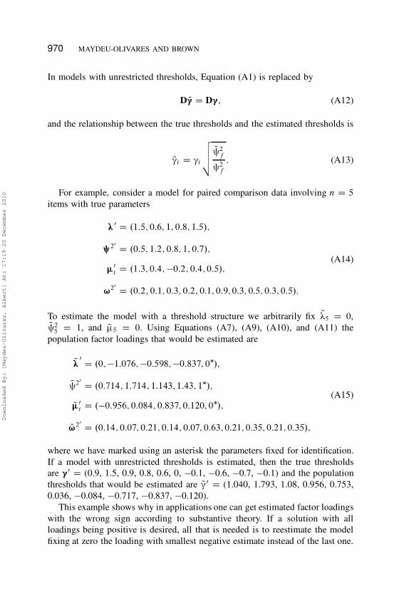
970 MAYDEU-OLIVARES AND BROWN
In models with unrestricted thresholds, Equation (A1) is replaced by
D Q” D D”; (A12)
and the relationship between the true thresholds and the estimated thresholds is
Q”i D ”i
v
u
u
t
Q§2f
§2f
: (A13)
For example, consider a model for paired comparison data involving n D 5
items with true parameters
œ0 D .1:5; 0:6; 1; 0:8; 1:5/;
§20 D .0:5; 1:2; 0:8; 1; 0:7/;
�0t D .1:3; 0:4; �0:2; 0:4; 0:5/;
¨20 D .0:2; 0:1; 0:3; 0:2; 0:1; 0:9; 0:3; 0:5; 0:3; 0:5/:
(A14)
To estimate the model with a threshold structure we arbitrarily fix Qœ5 D 0,Q§2
5 D 1, and Q�5 D 0. Using Equations (A7), (A9), (A10), and (A11) the
population factor loadings that would be estimated are
Qœ0 D .0; �1:076; �0:598; �0:837; 0�/;
Q§20 D .0:714; 1:714; 1:143; 1:43; 1�/;
Q�0t D .�0:956; 0:084; 0:837; 0:120; 0�/;
Q 20 D .0:14; 0:07; 0:21; 0:14; 0:07; 0:63; 0:21; 0:35; 0:21; 0:35/;
(A15)
where we have marked using an asterisk the parameters fixed for identification.
If a model with unrestricted thresholds is estimated, then the true thresholds
are ”0 D (0.9, 1.5, 0.9, 0.8, 0.6, 0, �0.1, �0.6, �0.7, �0.1) and the population
thresholds that would be estimated are Q”0 D (1.040, 1.793, 1.08, 0.956, 0.753,
0.036, �0.084, �0.717, �0.837, �0.120).
This example shows why in applications one can get estimated factor loadings
with the wrong sign according to substantive theory. If a solution with all
loadings being positive is desired, all that is needed is to reestimate the model
fixing at zero the loading with smallest negative estimate instead of the last one.
Downloaded By: [Maydeu-Olivares, Albert] At: 17:19 20 December 2010
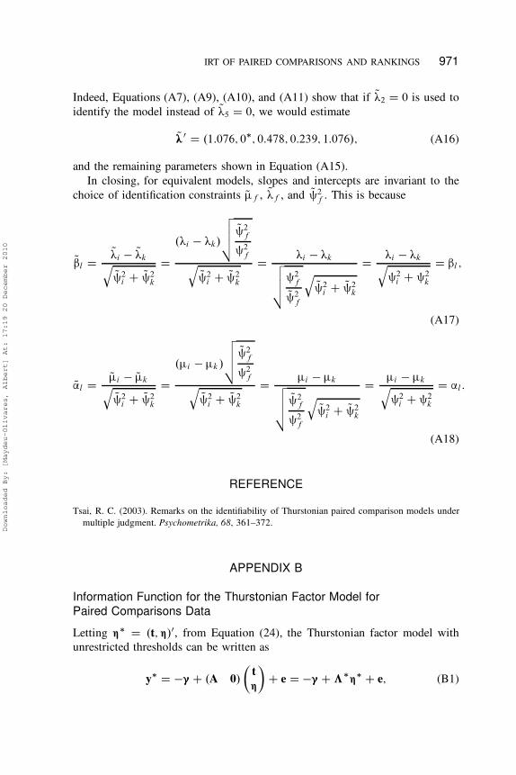
IRT OF PAIRED COMPARISONS AND RANKINGS 971
Indeed, Equations (A7), (A9), (A10), and (A11) show that if Qœ2 D 0 is used to
identify the model instead of Qœ5 D 0, we would estimate
Qœ0 D .1:076; 0�; 0:478; 0:239; 1:076/; (A16)
and the remaining parameters shown in Equation (A15).
In closing, for equivalent models, slopes and intercepts are invariant to the
choice of identification constraints Q�f , Qœf , and Q§2f . This is because
Q“l DQœi � Qœk
q
Q§2i C Q§2
k
D.œi � œk/
v
u
u
t
Q§2f
§2f
q
Q§2i C Q§2
k
D œi � œkv
u
u
t
§2f
Q§2f
q
Q§2i C Q§2
k
D œi � œkq
§2i C §2
k
D “l ;
(A17)
Q’l D Q�i � Q�kq
Q§2i C Q§2
k
D.�i � �k/
v
u
u
t
Q§2f
§2f
q
Q§2i C Q§2
k
D �i � �kv
u
u
t
Q§2f
§2f
q
Q§2i C Q§2
k
D �i � �kq
§2i C §2
k
D ’l :
(A18)
REFERENCE
Tsai, R. C. (2003). Remarks on the identifiability of Thurstonian paired comparison models under
multiple judgment. Psychometrika, 68, 361–372.
APPENDIX B
Information Function for the Thurstonian Factor Model for
Paired Comparisons Data
Letting ˜� D .t; ˜/0, from Equation (24), the Thurstonian factor model with
unrestricted thresholds can be written as
y� D �” C .A 0/
�
t
˜
�
C e D �” C ƒ�˜� C e; (B1)
Downloaded By: [Maydeu-Olivares, Albert] At: 17:19 20 December 2010
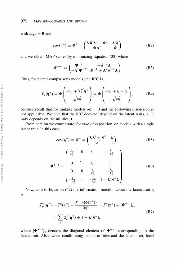
972 MAYDEU-OLIVARES AND BROWN
with �˜� D 0 and
cov.˜�/ � ˆ� D�
ƒˆƒ0 C ‰2 ƒˆ
ˆƒ0 ˆ
�
(B2)
and we obtain MAP scores by minimizing Equation (38) where
ˆ��1 D�
‰�2 �‰�2ƒ
�ƒ0‰�2 ˆ�1 C ƒ0‰�2ƒ
�
(B3)
Thus, for paired comparisons models, the ICC is
Pl .˜�/ D ˆ
0
B
@
�”l C œ�0
l ˜�
q
¨2l
1
C
AD ˆ
0
B
@
�”l C ti � tkq
¨2l
1
C
A; (B4)
because recall that for ranking models ¨2l D 0 and the following discussion is
not applicable. We note that the ICC does not depend on the latent traits, ˜. It
only depends on the utilities, t.
From here on we concentrate, for ease of exposition, on models with a single
latent trait. In this case,
cov.˜�/ � ˆ� D�
œœ0 C ‰2 œ
œ0 1
�
; (B5)
ˆ��1 D
0
B
B
B
B
B
B
B
B
@
1
§21
0 0 � œ1
§21
0:: : 0
:::
0 0 1§2
n� œn
§2n
� œ1
§21
� � � � œn
§2n
1 C œ0‰2œ
1
C
C
C
C
C
C
C
C
A
: (B6)
Now, akin to Equation (42) the information function about the latent trait ˜
is
I˜P .˜�/ D I
˜.˜�/ � @2 ln.¥.˜�//
@˜2D I
˜.˜�/ C Œˆ��1�˜;
DX
l
I˜
l .˜�/ C 1 C œ0‰2œ
(B7)
where Œˆ��1�˜ denotes the diagonal element of ˆ��1 corresponding to the
latent trait. Also, when conditioning on the utilities and the latent trait, local
Downloaded By: [Maydeu-Olivares, Albert] At: 17:19 20 December 2010
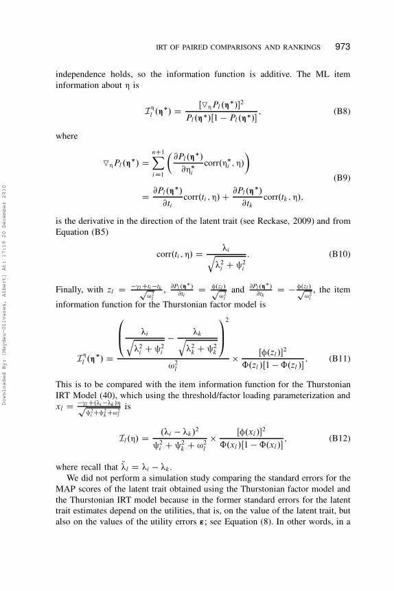
IRT OF PAIRED COMPARISONS AND RANKINGS 973
independence holds, so the information function is additive. The ML item
information about ˜ is
I˜
l .˜�/ D ŒO˜Pl .˜�/�2
Pl.˜�/Œ1 � Pl .˜�/�; (B8)
where
O˜Pl .˜�/ D
nC1X
iD1
�
@Pl.˜�/
@˜�i
corr.˜�i ; ˜/
�
D @Pl.˜�/
@ticorr.ti ; ˜/ C @Pl.˜
�/
@tkcorr.tk ; ˜/;
(B9)
is the derivative in the direction of the latent trait (see Reckase, 2009) and from
Equation (B5)
corr.ti ; ˜/ D œiq
œ2i C §2
i
: (B10)
Finally, with zl D �”l Cti �tkp¨2
l
,@Pl .˜
�/
@tiD ¥.zl /p
¨2l
and@Pl .˜
�/
@tkD � ¥.zl /p
¨2l
, the item
information function for the Thurstonian factor model is
I˜
l .˜�/ D
0
B
@
œiq
œ2i C §2
i
� œkq
œ2k C §2
k
1
C
A
2
¨2l
� Œ¥.zl /�2
ˆ.zl /Œ1 � ˆ.zl /�; (B11)
This is to be compared with the item information function for the Thurstonian
IRT Model (40), which using the threshold/factor loading parameterization and
xl D �”l C.œi �œk /˜p§2
i C§2k C¨2
l
is
Il.˜/ D .œi � œk/2
§2i C §2
k C ¨2l
� Œ¥.xl /�2
ˆ.xl /Œ1 � ˆ.xl /�; (B12)
where recall that Mœl D œi � œk.
We did not perform a simulation study comparing the standard errors for the
MAP scores of the latent trait obtained using the Thurstonian factor model and
the Thurstonian IRT model because in the former standard errors for the latent
trait estimates depend on the utilities, that is, on the value of the latent trait, but
also on the values of the utility errors ©; see Equation (8). In other words, in a
Downloaded By: [Maydeu-Olivares, Albert] At: 17:19 20 December 2010
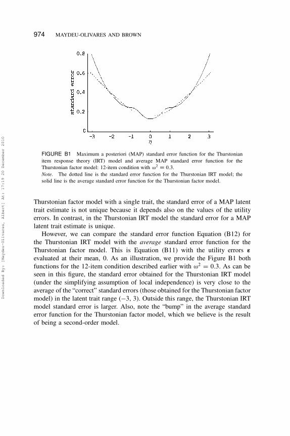
974 MAYDEU-OLIVARES AND BROWN
FIGURE B1 Maximum a posteriori (MAP) standard error function for the Thurstonian
item response theory (IRT) model and average MAP standard error function for the
Thurstonian factor model: 12-item condition with ¨2 D 0:3.
Note. The dotted line is the standard error function for the Thurstonian IRT model; the
solid line is the average standard error function for the Thurstonian factor model.
Thurstonian factor model with a single trait, the standard error of a MAP latent
trait estimate is not unique because it depends also on the values of the utility
errors. In contrast, in the Thurstonian IRT model the standard error for a MAP
latent trait estimate is unique.
However, we can compare the standard error function Equation (B12) for
the Thurstonian IRT model with the average standard error function for the
Thurstonian factor model. This is Equation (B11) with the utility errors ©
evaluated at their mean, 0. As an illustration, we provide the Figure B1 both
functions for the 12-item condition described earlier with ¨2 D 0:3. As can be
seen in this figure, the standard error obtained for the Thurstonian IRT model
(under the simplifying assumption of local independence) is very close to the
average of the “correct” standard errors (those obtained for the Thurstonian factor
model) in the latent trait range (�3, 3). Outside this range, the Thurstonian IRT
model standard error is larger. Also, note the “bump” in the average standard
error function for the Thurstonian factor model, which we believe is the result
of being a second-order model.
Downloaded By: [Maydeu-Olivares, Albert] At: 17:19 20 December 2010