itep-th-32/13 - arxiv
TRANSCRIPT

arX
iv:1
309.
2557
v5 [
hep-
th]
1 J
an 2
018
ITEP-TH-32/13
Lecture notes on interacting quantum fields in de Sitter space
E.T. Akhmedov1
Institute for Theoretical and Experimental Physics
117218, ul. B.Cheremushkinskaya, 25, Moscow
and
Moscow Institute of Physics and Technology
141700,Institutskii per. 9, Dolgoprudny, Moscow region
and
Mathematical Faculty of the
National Research University Higher School of Economics
117312, Vavilova 7, Moscow
Abstract
We discuss peculiarities of quantum fields in de Sitter space on the example of the self-interacting
massive real scalar, minimally coupled to the gravity background. Non-conformal quantum field
theories in de Sitter space show very special infrared behavior, which is not shared by quantum
fields neither in flat nor in anti-de-Sitter space: in de Sitter space loops are not suppressed in
comparison with tree level contributions because there are strong infrared corrections. That is
true even for massive fields. Our main concern is the interrelation between these infrared effects,
the invariance of the quantum field theory under the de Sitter isometry and the (in)stability of de
Sitter invariant states (and of dS space itself) under nonsymmetric perturbations.
Key words: de Sitter space, quantum fields in curved space-time, particle creation
PACS numbers: 04.62.+v, 98.80.Bp, 98.80.Cq, 98.80.Jk, 98.80.Qc
1 E–mail: [email protected]
2
Contents
I. Introduction 4
A. Motivation 4
B. General physical explanation of our main statements 5
II. de Sitter geometry 9
A. Global de Sitter metric 11
B. Penrose diagram 12
C. Expanding and contracting Poincare patches 13
D. Other de Sitter metrics and patches 15
E. Spatial volume in de Sitter space 16
III. Free scalar fields in de Sitter space 16
A. Free waves in Poincare patches 16
B. Digression on particle interpretation in de Sitter space 18
C. Free waves in global de Sitter space 20
D. Green functions in de Sitter space 21
1. Two-point correlation functions in global de Sitter space 22
2. Two-point correlation functions in the Poincare patches 23
E. Digression on an alternative quantization 24
IV. Loops in de Sitter space QFT 25
A. Brief introduction to the Schwinger–Keldysh diagrammatic technique 25
B. On de Sitter isometry invariance at loop level 30
C. One–loop correction in the expanding Poincare patch 32
1. Bunch–Davies vacuum 35
2. Contributions to the retarded and advanced propagators and to the vertices 36
3. Other α-harmonics 38
D. One-loop correction in the contracting Poincare patch 39
E. One-loop correction in global de Sitter space 40
V. Summation of leading infrared contribution in all loops 43
A. From the Dyson–Schwinger to the kinetic equation in the Poincare patches 44
1. Physical meaning of infrared effects 47
2. The kinetic equation 49
B. Solution of the kinetic equation in the Poincare patches 50
C. Kinetic equation in global de Sitter space 54
VI. Sketch of the results for λφ4 theory (instead of conclusions) 55
VII. Acknowledgements 57

3
References 57

4
I. INTRODUCTION
D-dimensional de Sitter (dS) space solves the general relativity (GR) equations of motion with
positive vacuum energy [1]:
Gαβ = −(D − 1)(D − 2)
2H2 gαβ , α, β = 0, . . . ,D − 1. (1)
Here Gαβ is the Einstein tensor and H is the Hubble constant. The signature of the metric, gαβ ,
is (−,+, . . . ,+). This space has a big isometry group, SO(D, 1), which is the analog of Poincare
invariance of Minkowski space.
Quantum effects produce an extra contribution, 〈Tαβ〉, to the right hand side of the GR equations
of motion. By 〈Tαβ〉 we denote the quantum average of the energy-momentum tensor of whatever
quantum fields are present on the dS background. What is the influence of this quantum average
on the background geometry? Our final goal is to answer this question. However, in these lectures
we concentrate on just a part of this program: We fix dS background and check whether the
assumption of negligible or small effects of 〈Tαβ〉 is selfconsistent.This quantum average, 〈Tαβ〉, contains the standard divergence due to zero-point fluctuations.
It is proportional to gαβ and should be absorbed into the ultraviolet (UV) renormalization of the
cosmological constant. Furthermore, quantum fields on the dS background are in a nonstationary
situation. Hence, nontrivial finite contributions to 〈Tαβ〉, such as, e.g., fluxes, can be present and
are of interest for us.
A. Motivation
It is natural to use the big isometry group of dS space in the formulation of quantum field
theory (QFT) on this background, i.e., it is appropriate to look for a dS-invariant state, if any,
and quantize excitations of such a state. (This is what one does when one quantizes fields on
Minkowski background: one explores the Poincare group.) But then, if the symmetry is respected
at all stages of quantization, correlation functions depend only on dS-invariant geodesic distances
rather than on each of their argument separately. Hence, in the free theory one can use the two-
point correlation function to find that all contributions to 〈Tαβ〉 are proportional to the metric,
gαβ . That is just a consequence of the symmetry in question. Furthermore, with the use of the
higher-point correlation functions one can extend this calculation to the interacting fields with the
same conclusion, if the dS isometry is also respected on loop level.
Thus, in the case of perfectly dS-symmetric situation, quantum effects just renormalize the
cosmological constant and dS space remains intact. Perhaps that is true unless exact correlators,
as functions of geodesic distances, show an explosive behavior. The main goal of these notes,
however, is to question the stability of dS space and to investigate if the dS isometry is broken
or the dS-invariant state is unstable with respect to nonsymmetric perturbations. It is probably
worth stressing here that in these notes we study just the behavior of correlation functions in dS

5
space and avoid using the notion of particle, unless this notion is meaningful and useful for the
interpretation of the obtained equations.
At tree level the situation is as follows: For massless scalar fields, which are minimally coupled
to the dS background, there is no Fock dS-invariant state [2], [3]. Also the very possibility to
define a dS-invariant state for gravity is still under discussion (see [4], [5]–[11], [12], [13], [14] and
[15]–[18]). All these interesting and important issues will not be touched in these lectures. We will
concentrate on the study of the real massive minimally coupled scalar field, φ. Then the situation
is conceptually simpler because in this case there is a one-parameter family of so-called α-vacua,
which respect the dS isometry at tree level [2], [19].
First, we would like to understand whether or not the dS isometry is respected by loop contri-
butions, if one quantizes over such a dS-invariant state: We will see that in some circumstances
the dS isometry is indeed broken. Second, in those circumstances, in which the dS isometry is
respected, we would like to understand whether or not the corresponding state is stable under
nonsymmetric perturbations. (Note that the vacuum is still dS-invariant. We just consider a non
trivial density matrix.) We find it physically inappropriate to consider the stability of any system
in a state in which all its symmetries are preserved. We will see that the exact dS-invariant state
does exist, but it is unstable under sufficiently strong nonsymmetric perturbations.
A few points are worth stressing. First, Minkowski space is stable under nonsymmetric particle
density perturbations over the Poincare invariant vacuum. That is just a consequence of the
energy conservation and of the H-theorem, neither of which is straightforwardly applicable in dS
space. Second, in the presence of nonsymmetric density perturbations, even tree level two-point
correlation functions depend on each of their arguments separately rather than on dS-invariant
distances between them. In view of what we have said here one can conclude that argumentation,
which is based on analytical properties of the correlators as functions of geodesic distances [20]–[24],
[25], [26], is not sufficient to support the stability of dS space.
For the other IR issues in dS space please see, e.g., [27]–[51].
B. General physical explanation of our main statements
To explain our statements let us briefly describe the dS geometry. dS space can be totaly
covered by the so-called global metric:
ds2 = −dt2 + cosh2(Ht)
H2dΩ2
D−1,
with dΩ2D−1 being the line element on the unit (D − 1)-dimensional sphere. At the same time the
inflationary (aka planar, aka spatially flat) metric is
ds2+ = −dτ2+ + e2Hτ+ d~x2+ =1
(Hη+)2[
−dη2+ + d~x2+]
, Hη+ = e−Hτ+ .

6
It covers only geodesically incomplete half of the whole space. The latter is referred to as the
expanding Poincare patch (EPP). The other half is referred to as the contracting Poincare patch
(CPP) and is covered by the metric
ds2− = −dτ2− + e−2Hτ− d~x2− =1
(Hη−)2[
−dη2− + d~x2−]
, Hη− = eHτ− .
The boundary between these patches (η± = +∞), which is simultaneously the initial Cauchy
surface of the EPP and the final one of the CPP, is light-like. One can obtain the CPP metric from
the EPP one by reflecting the direction of the conformal time, η+ ∈ (+∞, 0) −→ η− ∈ (0,+∞).
The EPP and CPP have a peculiarity in their geometry. The spatial part of their metric has
the conformal factor 1/η2±. Due to its presence every wave experiences strong blue shift towards
the past (future) infinity of the EPP (CPP). I.e., these regions of the Poincare patches correspond
to the UV limit.
In loop integrals on the EPP background the vertex integration goes over the half of dS space.
Hence, naively the dS isometry should be broken because there are generators of this symmetry
which can move the EPP within the whole dS space. However, following the original work [52], in
these lectures we will show that the dS isometry can indeed be respected in the loops, but only
if one starts exactly with the so-called Bunch–Davies (BD) state at the past infinity of the EPP.
BD is such a state that there are no positive energy excitations at the past (future) infinity of
the EPP (CPP) [53], [54]. In the region of dS space near the boundary between the EPP and
CPP one can define what one means by particle and what one means by positive energy. This
is possible because, as we have explained above, every momentum experiences infinite blue shift
towards the past (future) of the EPP (CPP). In fact, high energy harmonics are not sensitive to
the comparatively small curvature of the background space and behave as if they are in flat space.
After a Bogolyubov rotation from the BD harmonics to other modes, corresponding to other
dS-invariant states from the aforementioned α-family, one mixes the positive and negative energy
states. That spoils the UV behavior of the correlation functions. As a result, any vacuum different
from the BD one violates the dS isometry in the loops, even though it respects the symmetry at
tree level.
Should one conclude then that the problem of the influence of massive scalar fields on the dS
geometry is solved? It seems that in the EPP one just has to quantize fields over the BD state. But
the solution of this problem is not yet complete because of large infrared (IR) effects: IR corrections
may become destructive in the presence of nonsymmetric density perturbations because they are
not suppressed in comparison with tree level contributions.
As we will explain, all QFTs in dS space, which are not conformally invariant2, share the
same characteristic property, which is not present in massive QFTs in flat or anti-dS spaces [55].
Obviously the UV limit of any meaningful QFT over the dS or anti-dS backgrounds should be the
same as in flat space, hence, all the differences appear in the IR limit. Large IR effects, due to
2 I.e., such QFTs, which can feel the difference between the flat space and conformally flat dS one.
7
their large scale nature, are sensitive to the boundary and initial conditions in various patches of
the entire space. Hence, they should be separately considered in the EPP, CPP and in global dS
space.
Also, the character of these IR contributions in dS space crucially depends on the relation
between the mass and the Hubble constant: If the mass of the scalar field is big, m/H > (D−1)/2,
then the corresponding harmonic functions oscillate and decay to zero, as η → 0. Scalar fields with
such masses are composing the so-called principal series of theories. At the same time, harmonic
functions of the scalars with small masses, 0 < m/H ≤ (D − 1)/2, homogeneously decay to zero,
as η → 0. The corresponding theories are composing the so-called complementary series.
We first describe the situation in the EPP and then continue with the CPP and global dS space.
Due to the spatial homogeneity of the EPP and also of the initial states that we consider, it is
natural to perform the partial Fourier transformation along ~x+ directions. Then, the two-point
correlation function of interest for us acquires the form D(p|η+, η′+) = 12
⟨
φ(η+, ~p), φ(η′+,−~p)
⟩
,
where ·, · is the anticommutator. In the nonstationary situation it is the appropriate object to
study and is referred to as the Keldysh propagator. As we review below, in the limit when the
system approaches future infinity, p η = p√
η+η′+ → 0, the correlation function in question receives
large corrections for any mass of the field.
E.g., for the λφ3 scalar field theory from the principal series the first loop contains terms which
are proportional to λ2ηD−1 log(pη) [56], [57]. The same linear logarithmic corrections are also
present in the second loop of λφ4 theory [58]. (The only difference between the φ3 and φ4 theories
is in the mass-dependent coefficients of these IR contributions.) At the same time, the fields from
the complementary series receive powerlike corrections, which are proportional to λ2ηD−1 (pη)−2ν ,
where parameter ν depends on the mass and 0 < ν < (D − 1)/2 [58].
Thus, on the one hand, because of the factor ηD−1 in front of every contribution, which is due
to the expansion of the spatial sections of the EPP, such loop corrections do not make the Keldysh
propagator singular3 in the limit η → 0. But, on the other hand, even if λ2 is very small the
corrections in question become comparable to tree level contributions, as pη → 0. Hence, one has
to sum the unsuppressed leading IR contributions from all loops.
Of course one should not worry about the stability of the EPP, if the dS isometry is respected.
But what if we consider some finite nonsymmetric density perturbation over the BD state at the
past infinity of the EPP? Due to the rapid expansion of the EPP it is usually believed that such
density perturbations would quickly fade away and, thus, one should not care about their negligible
influence on the background geometry. However, the situation is quite counterintuitive because the
loop contributions go into the factor multiplying ηD−1 and marginally depend on the expansion
and/or contraction of spatial sections.
Let us clarify this observation here. The common wisdom is that excitations in the EPP can
reproduce themselves only very slowly. (It is believed that the reproduction should be at most
linear in time, e.g., due to the constant particle creation caused by the background field.) At the
3 Note that the only possible exception is given by the massless minimally coupled scalar field theory [33], [46], forwhich ν = (D − 1)/2.

8
same time, the expansion of the spatial sections is exponential and, hence, will rapidly win over
such a reproduction.
However, let us look more carefully at what is actually happening. Suppose we are in a situation
where one can give a meaning to the notion of particle in the future infinity of the EPP. (We will
see that this is possible under some conditions.) Then, consider, e.g., a particle dust in the EPP.
Its density per physical volume is indeed rapidly decreasing. However, the density per comoving
volume remains constant. (The comoving density is actually one of the quantities contributing to
the factor multiplying ηD−1 in the two-point correlation function under consideration.) Suppose
now there is some constant particle production process, i.e., it is the density per comoving volume
which is linearly growing. (That is what we will actually see.) Then, sooner or later it will become
very large and one will not be able to neglect the nonlinear particle self-reproduction processes.
We will see that the non-linearities are proportional to the density per comoving volume rather
than to that per physical one. (It may sound as very weird, but note that we are talking about
waves whose size is growing with time and even redshifted outside the cosmological horizon in the
progress towards future infinity.) As we will see, the nonlinear self-reproduction can actually cause
the destruction and win over the expansion.
Although we just perform the calculation of loop contributions to correlation functions, the
summation of unsuppressed IR loop corrections allows the particle interpretation and is related
to the above described particle kinetics. That happens to be true at least for the fields from
the principal series. We are not yet able to perform the summation of the IR divergences for the
complementary series because their physical meaning is not yet clear to us. But on general physical
grounds we expect that the IR effects in this case will be even stronger.
To sum unsuppressed IR loop corrections one has to find an IR solution of the system of Dyson–
Schwinger (DS) equations for the vertices, propagators and self-energies. We show, however, that
in the limit under study only the equation for the Keldysh propagator is relevant. Furthermore,
for the principal series it reduces to a kinetic equation of Boltzmann type, where plane waves are
substituted by exact dS harmonics. (As is known in condensed matter theory, loop effects may
become classical. That is related to the fact that loop corrections are not suppressed in comparison
with tree level contributions (see, e.g., [59], [60]).)
All elements of the kinetic equation that we obtain have a clear physical interpretation and
describe various particle decay and creation processes in the future infinity of the EPP [57], [61],
[62]. Moreover, we can find solutions of this kinetic equation for various initial conditions which
are set up by the initial (tree level) Keldysh propagator. One of the solutions shows an explosive
behavior of the two-point correlation function.
What about IR effects in the CPP and global dS? If we consider an exactly spatially homoge-
neous initial state, the loop calculation in the CPP follows straightforwardly from the one in the
EPP. Note, however, that unlike the EPP, the spatially homogeneous state in the CPP is unstable
with respect to the inhomogeneous perturbations. But it is still instructive to study loop effects in
such an ideal situation.
The metric in the CPP is identical to the one in the EPP if one reverses the direction of the
conformal time. But then, for the same reason as we have observed large IR contributions in the

9
EPP, there are IR divergences in the CPP: For the scalar fields from the principal series with the
λφ3 self-interaction the corrections are proportional to λ2ηD−1 log(η/η0), if pη ≪ 1. At the same
time, if pη ≫ 1, the corrections are proportional to λ2ηD−1 log(pη0). Here η ≡√
η−η′−, η0 is the
moment of time at past infinity, pη0 → 0, after which self-interactions are adiabatically turned
on. The same linear logarithmic contributions, but with different mass-dependent coefficients,
appear also in the second loop in the theory with λφ4 self-interaction [58]. For the scalars from
the complementary series the divergences are powerlike.
If it were not for the presence of the IR cutoff, η0, the loop integrals in the CPP would be
explicitly divergent: η0 cannot be taken to past infinity. Thus, one has to have an initial Cauchy
surface at some finite η0. But such a surface can be moved within the dS space by an isometry
transformation. Then, holding η0 fixed breaks the dS isometry and correlation functions start to
depend separately on each of their time arguments. Furthermore, the summation of the leading
IR contributions in the CPP is performed similarly to the EPP case. In fact, the kinetic equation
in the CPP is obtained from the one in the EPP just by the time reversal.
To study the situation in global dS space one has to keep in mind that it is the union of the
CPP and EPP. Hence, loops in global dS also have explicit IR divergences that break the dS
isometry [56], [62]. In this case it is also possible to derive the kinetic equation for the fields from
the principal series. But unlike the EPP and CPP case, this kinetic equation does not possess
an obvious quasi-particle description in the IR limit and we do not expect to have a stationary
solution in global dS, unless one considers a small enough part of it.
To conclude, the statements that we are going to advocate in these lectures are as follows. First,
we will observe that the only way to respect the dS isometry in loop contributions is to start at
the past infinity of the EPP exactly with the BD state. Any other dS-invariant vacuum, i.e., that
state which respects the dS isometry at tree level, does break it at loop level. Second, we will see
that any invariant initial state, including the so-called Euclidian one, in global dS space violates
the isometry in loops, due to IR divergences of loop integrals. Similarly, due to IR divergences,
any invariant initial state in the CPP also violates the dS isometry in loop contributions. And
finally, after the summation of unsuppressed IR contributions for the principal series in all loops,
we will proceed to show that even the BD state in the EPP is unstable under sufficiently strong
nonsymmetric perturbations. For the complementary series we expect even more destructive IR
effects, but we are not yet able to perform the loop summation.
The new content of these notes is mostly based on our previous work [57], [58], [61], [62].
II. DE SITTER GEOMETRY
D-dimensional dS space can be realized as hyperboloid,
−(
X0)2
+(
X1)2
+ · · ·+(
XD)2 ≡ gAB X
AXB = H−2, A,B = 0, . . . ,D, (2)
placed into the ambient (D + 1)-dimensional Minkowski space, with metric ds2 = gAB dXA dXB .
One way to see that a metric on such a hyperboloid solves equation (1) is to observe that it can

10
Figure 1: Each constant X0 slice of this two-dimensional dS space is a circle of radius (H−2 +X20 ).
be obtained from the sphere via the analytical continuation XD+1 → iX0. For illustrative reasons
we depict two-dimensional dS space on fig. 1.
Another way to see that the hyperboloid in question has a constant curvature is to observe that
eq. (2) is invariant under SO(D, 1) Lorentz transformations of the ambient space. The stabilizer of
any point obeying (2) is SO(D − 1, 1) group. Hence, dS is homogeneous, SO(D, 1)/SO(D − 1, 1),
space and any its point is equivalent to another one. Furthermore, all directions at every point are
equivalent. (Compare this with the sphere, which is SO(D+1)/SO(D).) Thus, SO(D, 1) Lorentz
group of the ambient Minkowski space is the dS isometry group.
The geodesic distance, L12, between two points, XA1 and XA
2 , on the hyperboloid can be con-
veniently expressed via the so-called hyperbolic distance, Z12, as follows:
cos (H L12)
H2≡ Z12
H2≡ gAB X
A1 X
B2 , where gAB X
A1,2X
B1,2 = H−2. (3)
To better understand the meaning of this expression, it is instructive to compare it to the geodesic
distance, l12, on a sphere of radius R:
R2 cos
(
l12R
)
≡ R2 z12 ≡(
~X1~X2
)
, where ~X21,2 = R2.
While the spherical distance, z12, is always less than unity, the hyperbolic one, Z12, can acquire
any value because of the Minkowskian signature of the metric.
11
All geodesics on the hyperboloid of Fig. (1) are curves that are cut out on it by planes going
through the origin of the ambient Minkowski space-time. (Compare this with the case of the
sphere.) Hence, space-like geodesics are ellipses, time-like ones are hyperbolas and light-like are
straight generatrix lines of the hyperboloid.
For every point XA on dS space, gAB XAXB = H−2, there is the antipodal one X
A= −XA,
which is just its reflection with respect to the origin in the ambient Minkowski space. Note that
then Z12 = −Z12.
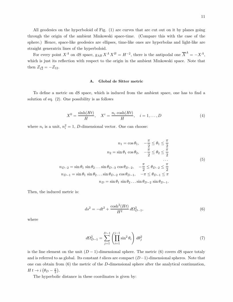
A. Global de Sitter metric
To define a metric on dS space, which is induced from the ambient space, one has to find a
solution of eq. (2). One possibility is as follows
X0 =sinh(Ht)
H, Xi =
ni cosh(Ht)
H, i = 1, . . . ,D (4)
where ni is a unit, n2i = 1, D-dimensional vector. One can choose:
n1 = cos θ1, −π2≤ θ1 ≤
π
2
n2 = sin θ1 cos θ2, −π2≤ θ2 ≤
π
2. . . (5)
nD−2 = sin θ1 sin θ2 . . . sin θD−3 cos θD−2, −π2≤ θD−2 ≤
π
2nD−1 = sin θ1 sin θ2 . . . sin θD−2 cos θD−1, −π ≤ θD−1 ≤ π
nD = sin θ1 sin θ2 . . . sin θD−2 sin θD−1.
Then, the induced metric is:
ds2 = −dt2 + cosh2(Ht)
H2dΩ2
D−1, (6)
where
dΩ2D−1 =
D−1∑
j=1
(
j−1∏
i=1
sin2 θi
)
dθ2j (7)
is the line element on the unit (D − 1)-dimensional sphere. The metric (6) covers dS space totaly
and is referred to as global. Its constant t slices are compact (D−1)-dimensional spheres. Note that
one can obtain from (6) the metric of the D-dimensional sphere after the analytical continuation,
H t→ i(
θD − π2
)
.
The hyperbolic distance in these coordinates is given by:

12
Figure 2: The standard quadratic Penrose diagram of D-dimensional dS space, when D > 2. The straight
thin line is the constant t and/or θ slice.
Z12 = − sinh(Ht1) sinh(Ht2) + cosh(Ht1) cosh(Ht2) cos(ω), (8)
where cos(ω) = (~n1, ~n2).
B. Penrose diagram
To understand the causal structure of dS space it is convenient to transform the global coordi-
nates as follows:
cosh2(Ht) =1
cos2 θ, −π
2≤ θ ≤ π
2
and to obtain the metric
ds2 =1
H2 cos2 θ
[
−dθ2 + dΩ2D−1
]
, (9)
which is conformal to that of the Einstein static universe, ds2ESU = −dθ2 + dΩ2D−1, with compact
time θ. The causal structure of the latter universe coincides with that of dS space because sign
of ds2 coincides with that of ds2ESU . Hence, one can drop the conformal factor and depict the

13
compact space. Such a procedure is just a variant of the stereographic projection. In the modern
language the result of the projection of a space-time is referred to as Penrose diagram.
If D > 2, then to draw the diagram on the two-dimensional sheet we should choose, in addition
to θ, one of the angles θj, j = 1, . . . ,D − 1. The usual choice is θ1 because the metric in question
has the form dθ2 + dθ21 + sin2(θ1)dΩ2D−2, i.e., it is flat in the (θ − θ1)-plain. The Penrose diagram
for dS space, whose dimension is grater than 2, is depicted on fig. 2.
Note that when D > 2 angle θ1 is taking values in the range[
−π2 ,
π2
]
. At the same time, when
D = 2 we have that θ1 ∈ [−π, π]. When D > 2, the problem with the choice of θ1 in the Penrose
diagram is that then cylindrical topology, SD−1 × R, of dS space is not transparent. At the same
time, the complication with the choice of θD−1 ∈ [−π, π], instead of θ1, appears form the fact
that the metric in the (θ − θD−1)-plain is not flat. For this reason we prefer to consider just the
stereographic projection in the two-dimensional case because it is sufficient to describe the causal
structure and also clearly shows the topology of dS space.
The Penrose diagram of the two-dimensional dS space is shown on fig. 3. This is the stereo-
graphic projection of the hyperboloid from fig. 1. What is depicted here is just a cylinder because
the left and right sides of the rectangle are glued to each other. The fat solid curve is a world line
of a massive particle. Thin straight lines, which compose 45o angle with both θ and θ1 axes, are
light rays. From this picture one can see that every observer has a causal diamond within which
he can exchange signals. Due to the expansion of dS space there are parts of it that are causally
disconnected from the observer.
C. Expanding and contracting Poincare patches
Another possible solution of (2) is based on the choice:
−(
HX0)2
+(
HXD)2
= 1−(
H xi+)2e2H τ+ ,
(
HX1)2
+ · · ·+(
HXD−1)2
=(
H xi+)2e2H τ+ . (10)
Then, one can define
HX0 = sinh (H τ+) +
(
H xi+)2
2eH τ+ ,
H Xi = Hxi+ eH τ+ , i = 1, . . . ,D − 1,
H XD = − cosh (H τ+) +
(
H xi+)
2eH τ+ . (11)
With such coordinates the induced metric is
ds2+ = −dτ2+ + e2H τ+ d~x2+. (12)
Note, however, that in (11) we have the following restriction: −X0 + XD = − 1H eH τ+ ≤ 0, i.e.,
metric (12) covers only half, X0 ≥ XD, of the entire dS space. It is referred to as the expanding

14
Figure 3: The rectangular Penrose diagram of the two-dimensional dS space. Note that the left and right
sides of this rectangle are glued to each other. Thus, while on fig. 2 the positions θ1 = ±π2sit at the opposite
poles of the spherical time slices, on the present figure the positions θ1 = ±π coincide.
Poincare patch (EPP). Another half of dS space, X0 ≤ XD, is referred to as the contracting
Poincare patch (CPP) and is covered by the metric
ds2− = −dτ2− + e−2H τ− d~x2−. (13)
In both patches it is convenient to change the proper time τ± into the conformal one. Then, the
EPP and CPP both possess the same metric:
ds2± =1
(H η±)2
[
−dη2± + d~x2±]
, H η± = e∓H τ± . (14)
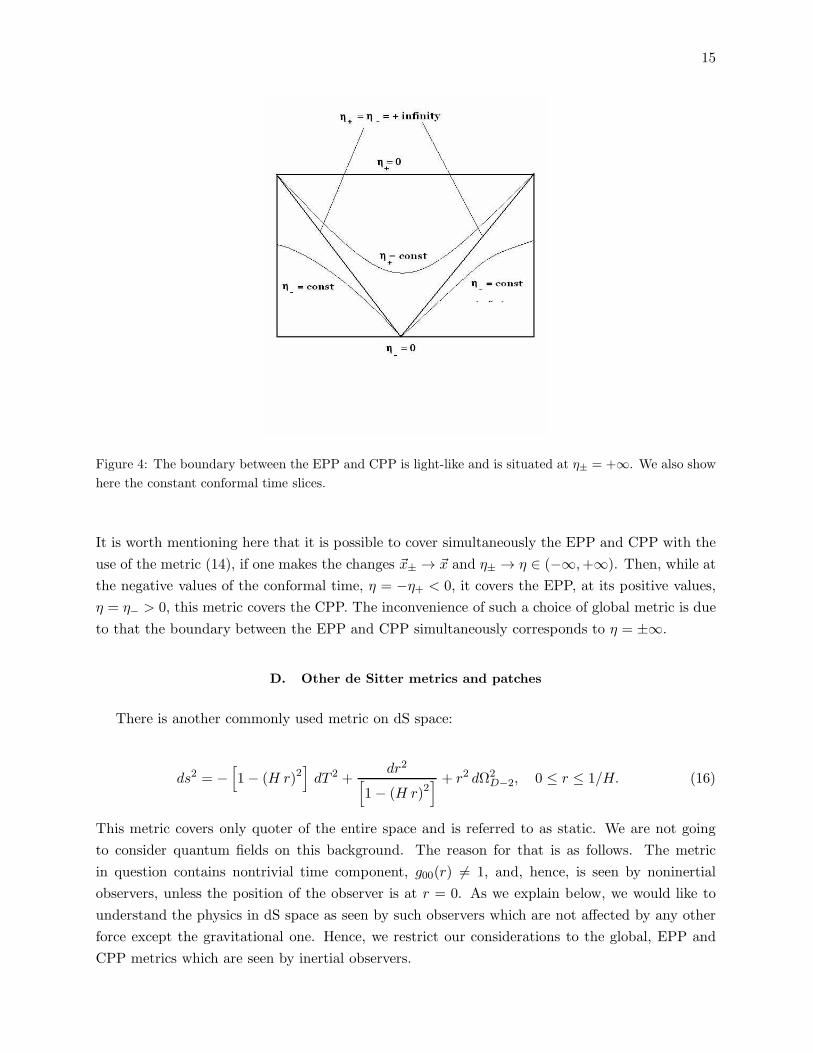
However, while in the EPP the conformal time is changing form η+ = +∞ at past infinity (τ+ =
−∞) to 0 at future infinity (τ+ = +∞), in the CPP the conformal time is changing from η− = 0 at
past infinity (τ− = −∞) to +∞ at future infinity (τ− = +∞). Both the EPP and CPP are shown
on fig. 4.
The hyperbolic distance in the EPP and CPP has the form:
Z12 = 1 +(η1 − η2)
2 − |~x1 − ~x2|22 η1 η2
(15)
15
Figure 4: The boundary between the EPP and CPP is light-like and is situated at η± = +∞. We also show
here the constant conformal time slices.
It is worth mentioning here that it is possible to cover simultaneously the EPP and CPP with the
use of the metric (14), if one makes the changes ~x± → ~x and η± → η ∈ (−∞,+∞). Then, while at
the negative values of the conformal time, η = −η+ < 0, it covers the EPP, at its positive values,
η = η− > 0, this metric covers the CPP. The inconvenience of such a choice of global metric is due
to that the boundary between the EPP and CPP simultaneously corresponds to η = ±∞.
D. Other de Sitter metrics and patches
There is another commonly used metric on dS space:
ds2 = −[
1− (H r)2]
dT 2 +dr2
[
1− (H r)2] + r2 dΩ2
D−2, 0 ≤ r ≤ 1/H. (16)
This metric covers only quoter of the entire space and is referred to as static. We are not going
to consider quantum fields on this background. The reason for that is as follows. The metric
in question contains nontrivial time component, g00(r) 6= 1, and, hence, is seen by noninertial
observers, unless the position of the observer is at r = 0. As we explain below, we would like to
understand the physics in dS space as seen by such observers which are not affected by any other
force except the gravitational one. Hence, we restrict our considerations to the global, EPP and
CPP metrics which are seen by inertial observers.
16
Note here that the transformation from the proper time, τ±, to the conformal one, η±, (which
makes g00 time-dependent) is nothing but the change of the clock rate rather than a transition to
the noninertial motion.
E. Spatial volume in de Sitter space
For our future considerations it is important to define here the physical and comoving spatial
volumes in global dS space and in its Poincare patches. The spatial sections in all aforementioned
metrics contain conformal factors, cosh2(H t)H2 or 1
(H η±)2. Then, there is the volume form, dD−1V , with
respect to the spatial metric, which is multiplying the corresponding conformal factor. This form
remains constant during the time evolution of the spatial sections and is referred to as comoving
volume.
It is important to observe that if one considers a dust in dS space, then its density per comoving
volume remains constant independently of whether spatial sections are expanding or contracting.
At the same time if one takes into account the conformal factor, i.e., the expansion (contraction)
of the EPP (CPP), then he has to deal with the physical volume, dD−1V±(H η±)D−1 . In global dS space the
physical volume iscoshD−1(H t) dD−1Vsphere
HD−1 . Of course the density of the dust with respect to such a
volume is changing in time.
III. FREE SCALAR FIELDS IN DE SITTER SPACE
We start our discussion with free massive real scalar fields which are coupled to the dS back-
ground in the minimal way. From now on we set the curvature of dS space to one, H = 1, and
assume it to be fixed. In the following sections we will question this assumption in the presence of
quantum effects in interacting theories.
A. Free waves in Poincare patches
The action of the free theory under consideration is as follows:
S =
∫
dDx√
|g|[
gαβ ∂αφ∂βφ+m2 φ2]
. (17)
In the EPP or CPP the Klein–Gordon (KG) equation is:
[
−η2∂2η + (D − 2) η ∂η + η2∆−m2]
φ(η, ~x) = 0, (18)
where ∆ is the (D−1)-dimensional flat Laplacian. At this point we do not distinguish the EPP from
the CPP and, hence, drop the “±” indexes of η and ~x. The harmonics, which solve this equation,
can be represented as φp(η, ~x) = gp(η) e∓i ~p ~x. If one assumes the ansatz gp(η) = η
D−12 h(pη),

17
where p = |~p|, then (18) reduces to the Bessel equation for h(pη). The index of this equation is
iµ = i
√
m2 −(
D−12
)2.
Generic solution of the Bessel equation with such an index behaves as follows:
h(x) =
A ei x√x+B e−i x√
x, x→ ∞
C xiµ +Dx−iµ, x→ 0(19)
Here A,B,C,D are some complex constants. Taking into account that (pη)±iµ ∼ e±i µ τ , one can
interpret x±i µ, if µ is real, as a single wave in the future (past) of the EPP (CPP).
If the field is heavy, m > (D − 1)/2, then, it belongs to the so-called principal series. The
corresponding gp harmonics oscillate and decay to zero as η(D−1)/2±iµ, when η → 0. At the same
time, for the light field from the complementary series, m ≤ (D − 1)/2, the harmonic functions
homogeneously decay to zero as η(D−1)/2±√
(D−1)2/4−m2, when η → 0. The only exception is the
massless field, m = 0, for which harmonics approach a non-zero constant in future infinity.
Bessel functions of the first, h(x) =√
πsinh(πµ) Jiµ(x), or second, h(x) ∝ Yiµ(x), kinds correspond
to those modes for which either C or D in (19) is vanishing. But then both A and B are not zero.
Thus, Bessel harmonics represent single free waves only in the future (past) infinity of the EPP
(CPP). Correspondingly they are referred to as out- (in-)harmonics in the EPP (CPP).
Performing a Bogolyubov transformation, one can consider also other possibilities for h(x). For
example, Hankel functions of the first, h(x) =√π2 e−
π µ2 H
(1)iµ (x), or second, h(x) =
√π2 e
π µ2 H
(2)iµ (x),
kinds are such that either A or B in (19) is vanishing. But then both C and D are not zero. Thus,
Hankels, which are referred to as Bunch–Davies (BD) modes [53], represent single free waves only
in the past (future) infinity of the EPP (CPP).
For the beginning we do not specify our choice for h(pη) because none of them behaves as single
wave simultaneously at past and future infinity. Then, quantum field can be mode expanded in
the usual way:
φ(η, ~x) =
∫
dD−1~p[
a~p gp(η) e−i ~p ~x + h.c.
]
, gp(η) = ηD−1
2 h(pη). (20)
Corresponding annihilation, a~p, and creation, a+~p , operators obey the proper Heisenberg commu-
tation relations. They follow from the commutation relations of φ with its conjugate momentum
and are the corollary of the time-independence of the Wronskian, η2−D(
gp g∗p − gp g
∗p
)
= ±i, whichfollows from the equations of motion. This observation allows to fix the proper normalization of
the harmonic functions.
For the illustrative reasons let us consider the free Hamiltonian in D = 4. In an arbitrary
dimension the formulas are similar. The Hamiltonian can be found from (17), using the machinery
presented, e.g., in Ref. [63]. The energy-momentum tensor is Tαβ = ∂αφ∂βφ − gαβL, where L
is the Lagrangian density. Then, the free Hamiltonian (before the normal ordering) is H0(η) =1η2
∫
d3xT00(η, ~x) and can be expressed via the creation and annihilation operators as:

18
H0(η) =
∫
d3p[
Ap(η) a+~p a~p +Bp(η) a~p a−~p + h.c.
]
,
Ap(η) =1
2η2
|gp|2 +[
p2 +m2
η2
]
|gp|2
,
Bp(η) =1
2η2
g2p +
[
p2 +m2
η2
]
g2p
, gp ≡dgpdη
. (21)
The main characteristic feature of this Hamiltonian is that one cannot diagonalize it once and
forever. That is because there is no solution of the KG equation which coincides with the function
that solves equation Bp(η) = 0. (In flat space the simultaneous solution of the corresponding KG
equation and of Bp = 0 is the plane wave.) Moreover, one cannot use such gp(η) which solve
Bp(η) = 0 equation in place of the mode functions in (20) because then the corresponding creation
and annihilation operators will not obey the appropriate Heisenberg algebra.
However, Bp(η) can be set to zero as η → +∞. This can be done if one chooses the BD modes
because they behave as single plane waves when η → +∞. Then, we have a clear meaning of the
positive energy and of the particle in this region of space-time because the Hamiltonian is diagonal.
Recalling that the past (future), η → +∞, of the EPP (CPP) corresponds to the UV limit of the
physical momentum, pη, one can see that other harmonics have wrong UV behavior. In fact, after
a Bogolyubov rotation of the BD modes to other harmonics one mixes positive and negative energy
excitations.
There are no modes that allow to set Bp(η) to zero as η → 0. That is because the gravitational
field is never switched off in this limit. In fact, Bp(η) does not asymptotically approach a constant
and one has to re-diagonalize the free Hamiltonian at each new value of η, as η → 0. (Note that in
the above UV limit the gravitational field is effectively switched off because high energy harmonics
are not sensitive to the comparatively small curvature of the background space.) Hence, naively
even the Bessel functions, out- (in-)modes, do not provide a proper quasi-particle description in
the future (past) infinity of the EPP (CPP).
B. Digression on particle interpretation in de Sitter space
It is probably worth stressing here that throughout these notes we will avoid using the notion
of particle, unless this notion is meaningful. We will concentrate on the behavior of the correlation
functions. However, let us make here some comments about the particle interpretation.
In curved space-times one usually avoids the use of the notion of particle because it is believed
to be an observer dependent phenomenon. In fact, different observers may detect different particle
fluxes. However, one should separate the Unruh effect [64] from what we would like to call as the
real particle production. In Minkowski space, both inertial and noninertial observers see the same
state — Minkowski (Poincare invariant) vacuum. However, while an inertial observer sees it as the
empty space, a noninertial one sees it as the thermal state. That is due to the specific correlation of
the vacuum fluctuations along its worldline [65], [66]. Note that there is no nontrivial gravitational

19
field present in the circumstances under consideration because in flat space the Riemanian tensor
is exactly zero.
The real particle creation is due to a change of the ground state under the influence of quantum
effects in a non-trivial background field. Then a flux is seen by all sorts of observers. That is
exactly what happens in the strong electric field, in dS space and in the collapsing background.
Rephrasing that, we would like to say here that, while in Minkowski space there is one type of
observers that does not see any particle flux, in dS space there is no such an observer that sees
nothing. On general grounds, we expect that the least flux is seen by inertial observers — they
do not see the extra Unruh type of flux, so to say. (Note here that the least possible flux in a
given space-time is an observer independent/invariant notion, i.e. is a characteristic feature of the
given space–time.) Apart from that, if we see strong backreaction in a noninertial frame it is not
clear whether it should be attributed to the background gravitational field or to the extra non-
gravitational force acting on the corresponding observer. While in an inertial frame the situation
is unambiguous.
In any case, independently of whatever name we use for different quantities that are calculated
below, all of them are just components of correlation functions. And at the end of the day the
objects that we calculate are just correlation functions. However, the notion of particle sometimes
is convenient for the physical interpretation of various equations that will appear below.
So, what do we mean by particle? In general if the free Hamiltonian of a theory is diagonal
then one indeed can have a particle interpretation. Furthermore, if for some reason the anomalous
quantum average 〈ap a−p〉 is strongly suppressed in comparison with 〈a+p ap〉 then one also can give
a meaning to particle like excitations, as we will see below.
Then, in principle at every given moment of time, η, one can make an instantaneous Bogolyubov
rotation as follows [68]:
b~p(η) = αp(η) a~p + βp(η) a+−~p, b+~p (η) = α∗
p(η) a+~p + β∗p(η) a−~p, (22)
with
αp(η) =
√
Ap +Ωp2Ωp
and βp(η) =B∗p
Ap +Ωpαp(η), (23)
where Ωp(η) =√
A2p − |Bp|2. The Hamiltonian (21) becomes diagonal
H0(η) =
∫
d3~pΩp(η)[
b+~p (η) b~p(η) + h.c.]
. (24)
The rotated harmonics are
gp(η) = α∗p gp − β∗p g
∗p =
i η[
p2 + m2
η2
]14
gp − i√
p2 + m2
η2 gp∣
∣
∣gp − i
√
p2 + m2
η2gp
∣
∣
∣
. (25)

20
This allows to have a particle interpretation around any given moment of time η.
Note that the new creation and annihilation operators, b~p and b+~p , depend on time η. But a~p
and a+~p are time independent in the free theory — all their time dependence is, then, gone into the
harmonics gp(η). They start to depend on time if one turns on interactions.
One reason to avoid using b’s is that if one knows all expressions in terms of a’s then it is not
hard to restor their form in terms of b’s. Another reason is that as we will see, if m > (D−1)/2, a’s
do provide a proper quasi-particle description in the IR limit. In fact, it will happen that for some
choice of harmonics, 〈ap a−p〉 is suppressed in comparison with 〈a+p ap〉, as the system approaches
future infinity. Hence, one does not really need to make the rotation to b’s.
C. Free waves in global de Sitter space
In global dS space the KG equation is as follows:
[
−∂2t + (D − 2) tanh(t) ∂t +∆D−1(Ω)
cosh2(t)−m2
]
φ(t,Ω) = 0. (26)
Here ∆D−1(Ω) is the (D − 1)-dimensional spherical Laplacian. The solution of this equation can
be represented as φj,~m(t,Ω) = gj(t)Yj,~m(Ω), where ∆D−1(Ω)Yj,~m(Ω) = −j (j + D − 2)Yj,~m(Ω),
and Yj,~m(Ω) are (D− 1)-dimensional spherical harmonics, ~m is the multi-index enumerating them
in the dimension grater than two.
The equation for gj(t), following from (26), can be reduced to the hypergeometric one. One
possible its solution is [67]:
g(in)j (t) =
2j+D2−1
õ
coshj(t) e(j+D−12
±i µ) t F
(
j +D − 1
2, j +
D − 1
2∓ i µ; 1∓ i µ;−e2 t
)
. (27)
Where, from now on, F (a, b; c;x) is the hypergeometric function of the (2, 1) type and µ was defined
in the previous subsection. These harmonics behave as single waves at the past infinity, t→ −∞,
of global dS space:
g(in)j (t) ∼ e
D−12
t e∓i µ t.
That is the reason why they are referred to as in-harmonics. At the same time, as t→ +∞, these
modes behave as
g(in)j (t) ∼ e
D−12
t(
C1 e∓i µ t + C2 e
±i µ t) ,
where C1,2 are both non-zero complex constants in even dimensional dS space. In odd dimensional
dS spaces C2 = 0 [67]. The out-harmonics in global dS are as follows g(out)j (t) =
[
g(in)j (−t)
]∗. Their
name is justified by the observation that they behave as single waves at future infinity.
21
Another peculiar type of harmonics in global dS space is given by the so-called Euclidian ones
[2], [19], [67]. They are defined as:
g(E)j (t) =
2j+D2−1 i−j+
D−12
õ
coshj(t) e(j+D−12
±i µ) t ×
×F(
j +D − 1
2, j +
D − 1
2± i µ; 2 j +D − 1; 1 + e2 t
)
(28)
and are regular on the lower hemisphere after the analytical continuation, t → i (θ − π/2). Then,
complete wave functions of the Euclidian modes obey φ(E)j,~m
(
X)
=[
φ(E)j,~m (X)
]∗, where X is the
antipodal point of X.
All the aforementioned mode functions in global dS space belong to the one-parameter family
of the so-called α-harmonics [2], [67]:
φ(α)j,~m(X) =
1√1− eα+α∗
[
φ(E)j,~m(X) + eα φ
(E)j,~m(X)
]
, (29)
where α is a complex number.
Note the coincidence, after the identification η∓ = e±t, of the above behavior of the global dS
harmonic functions with that of the modes at the past and future of the CPP and EPP. In fact,
under such an identification the metric of global dS space at its past and future infinity can be
well approximated by those of the CPP and EPP, correspondingly. Hence, there is a one-to-one
correspondence between harmonic functions in the EPP (CPP) and α-modes in global dS.
The free Hamiltonian of the four-dimensional theory can be written as:
H0(t) =1
2
∑
j,~m
[
Aj(t) a+j,~m aj,~m +Bj(t) aj,~m aj,−~m + h.c.
]
,
Aj(t) =cosh3(t)
2
|gj |2 +[
L (L+ 2)
cosh2(t)+m2
]
|gj |2
,
Bj(t) =cosh3(t)
2
g2j +
[
L (L+ 2)
cosh2(t)+m2
]
g2j
× (a phase) . (30)
There is no choice of harmonics which allows to diagonilize this Hamiltonian neither in the past
nor in the future infinity because in global dS space the background field is never switched off. In
fact, Bj(t) does not approach a constant neither in the past nor in the future infinity of global dS
space.
D. Green functions in de Sitter space
We continue with the construction of two-point correlation functions. The Wightman function,
〈φ(X1)φ(X2)〉, is a solution of the homogeneous KG equation:(
−m2)
G (X1,X2) = 0. Because
of the dS isometry invariance, it should be a function of the invariant distance between X1 and X2.
The KG operator,(
−m2)
, when acting on a function of Z = Z12 can be reduced to [19], [2]:

22
[(
Z2 − 1)
∂2Z +DZ ∂Z +m2]
G(Z) = 0. (31)
This equation coincides with that for the Wightman function on the D-dimensional sphere. We just
have to keep in mind that in the latter case Z is the spherical distance rather than the hyperbolic
one. The same equation is also valid in anti-dS and Euclidian anti-dS (Lobachevsky) space. One
just has to change the sign of m2 term, due to the change of the sign of the curvature H2, and
keep in mind that Z is the hyperbolic distance in the corresponding space.
Eq. (31) has three singular points Z = ±1,∞ in the complex Z-plain. Hence, it is not hard
to recognize in it the hypergeometric equation. After the transformation to the new variable,
z = (1 + Z)/2, one puts the singular points into their standard positions, z = 0, 1,∞. Then, the
generic solution of this equation is:
GW (Z) = A1 F
(
D − 1
2+ i µ,
D − 1
2− i µ;
D
2;1 + Z
2
)
+
+A2 F
(
D − 1
2+ i µ,
D − 1
2− i µ;
D
2;1− Z
2
)
. (32)
Here A1,2 are some complex constants and µ was defined above. The two hypergeometric functions
in (32) behave, when Z → ±1, as follows:
F
(
D − 1
2+ i µ,
D − 1
2− i µ;
D
2;1± Z
2
)
∼ 1
(1∓ Z)D2−1. (33)
Also they have the branching point at Z → ∞:
GW (Z) ∼ B+ Z−D−1
2+i µ +B− Z
−D−12
−i µ.
Here B± are some complex constants which depend on A1,2. Thus, GW (Z) is an analytical function
on the complex Z-plain with two branch cuts going from Z = ±1 to infinity.
What is the physical meaning of the singularities that GW (Z) has? Is there any state for which
GW (Z) looks as in (32)? We are going to address these questions now.
1. Two-point correlation functions in global de Sitter space
We first scetch the situation in global dS and then continue with a bit more extensive discussion
of the EPP (CPP) case. We choose some solution of the corresponding KG equation and, thus,
specify α-modes. Then, we define the α-vacuum as the state which is annihilated by the corre-
sponding annihilation operators: a(α)j,~m |α〉 = 0. For every choice of α there is the corresponding
α-vacuum [2]. Then, one can construct the two point Wightman function as
Gα (X1,X2) ≡ 〈α |φ(X1)φ(X2)|α〉 ,

23
where he has to substitute the α-harmonic expansion of φ(X). It is straightforward to show (using,
e.g., [70]) that away from its singularity points this function looks as (32) with such A1,2 which
depend on α. At the same time Z = Z12 is the hyperbolic distance, which is expressed via the
global coordinates of X1 and X2.
For the Euclidian vacuum we have that A2 = 0 and the singularity point of the corresponding
Wightman function GE(Z12) is at Z12 = 1. From (33) one can see that it is the standard UV
behavior, when X1 is sitting on the light-cone whose apex is at X2. The demand that this UV
singularity should be the same as in flat space allows to fix simultaneously the A1 coefficient in
(32) and the ǫ-prescription (the resolution of the singularity):
GE(Z) = G (Z − i ǫ sign∆t) , where
G(Z) ≡ Γ(
D−12 + i µ
)
Γ(
D−12 − i µ
)
(4π)D2 Γ
(
D2
)
F
(
D − 1
2+ i µ,
D − 1
2− i µ;
D
2;1 + Z
2
)
. (34)
The same value of A1 also follows from the proper normalization of the Euclidian harmonics.
The ǫ-prescription for the α-harmonics follows after the Bogolyubov rotation (29). The result
is as follows [67]:
Gα(Z) =1
1− eα+α∗
[
G (Z − i ǫ sign∆t) + eα+α∗
G (Z + i ǫ sign∆t)+
+eα∗
G (−Z + i ǫ sign∆t) + eαG (−Z − i ǫ sign∆t)]
, (35)
where G(Z) is defined in (34). If one puts ǫ = 0 in this expression, he can reproduce (32) with
generic A1,2.
At the same time ǫ-prescription for the T-ordered (Feynman) propagator in the Euclidian vac-
uum is GT (Z) = G (Z − i ǫ). This correlation function is just the analytical continuation of the
propagator on the sphere in the complex Z-plain.
2. Two-point correlation functions in the Poincare patches
To define the Wightman function in the EPP or CPP, one also has to pick up a solution of the
Bessel equation and define the corresponding vacuum, a~p |vac〉 = 0. Then, doing the same as it
was done above, one obtains the Fourier expansion of the correlation function:
GW (X1,X2) =
∫
dD−1~p ei ~p (~x1−~x2) (η1 η2)D−1
2 h(pη1)h∗(pη2). (36)
Using [70], one can calculate this integral for different choices of h(pη). 6.672.1-4 of [70] can be used
for the calculation in the case of 2D, and generalizations to higher dimensions are straightforward.
There are two conclusions that follow. First one is that GW depends on the invariant hyperbolic
distance Z12 expressed via η1,2 and ~x1,2 as (15). And the second one is that different solutions of

24
the Bessel equation, h(pη), are in one–to–one correspondence with the concrete values of A1,2 in
(32) [2].
In particular, for the BD state we have that A2 = 0. Thus, this state in the EPP and CPP
leads to the same propagator as the Euclidian state in global dS space. Then, for the BD state
the singularity of GW (Z) is at Z = 1 and corresponds to the UV limit of the physical momentum,
pη → ∞. Hence, similarly to the flat space case, for the integral in (36) to be properly defined at
the singularity, there should be an appropriate shift as follows: η1 − η2 → η1 − η2 ± i ǫ. The sign
of this shift depends on which one among η1 or η2 is grater than the other. Thus, the Wightman
function in the BD state is also defined by (34). The difference is that now Z12 is expressed via
the EPP (CPP) coordinates of X1 and X2 and ∆t should be substituted by ∓∆η±. Here the “−”
sign for the EPP is due to the reverse order of the time flow.
After a Bogolyubov rotation to other modes in the EPP (CPP) A2 becomes nonzero and A1
is changed. Thus, the residue of the singularity at Z12 = 1 is changed and also appears another
singularity at Z12 = −1. Recalling that Z12 = −Z12, one can conclude that another singularity
corresponds to the situation when X1 is sitting on the light-cone with the apex at X2 — antipodal
point of X2. This singularity is causally disconnected from the one at Z12 = 1. In fact, a light ray
passing through any point X on the hyperboloid on fig. 1 is a generatrix of this hyperboloid. Two
generatrix lines crossing at X2 never intersect those which are crossing at X2. This can be seen
from the Penrose diagram.
Thus, for the other harmonics in the EPP and CPP the Wightman functions are also given by
(35), where instead of the Euclidian harmonics in (29) one should use the BD ones.
E. Digression on an alternative quantization
There is a different way of field quantization in dS space4. While in flat space this procedure
leads to the same result, in dS space it provides an alternative quantization.
Consider for the illustrative reasons two-dimensional scalar field in global dS space:
S =1
2
∫
dt
∫ 2π
0dθ cosh(t)
[
−φ2 +m2φ2 +1
cosh2(t)(∂θφ)
2
]
. (37)
Let us Fourier expand the field in the spatial direction φ(t, θ) =∑+∞
p=−∞ gp(t) ei p θ, where gp obeys
the condition gp = g∗−p because φ is real. In terms of gp the Lagrangian is:
L = π+∞∑
p=0
cosh(t)
[
gp g∗p −
(
m2 +p2
cosh2(t)
)
gp g∗p
]
. (38)
If one defines gp = 1√4π
(qp + iQp), M(t) = cosh(t) and ω2p(t) = m2 + p2
cosh2(t), then he can write
the corresponding Hamiltonian as follows:
4 I would like to thank V.Losyakov and A.Morozov for the discussions on this issue.
25
H0 =
+∞∑
p=0
[
1
2M(t)
(
p2p + P 2p
)
+M(t)ω2
p(t)
2
(
q2p +Q2p
)
]
. (39)
Here pp and Pp are momenta conjugate to qp and Qp, correspondingly. Then, via the definition of
the operators
ap =1√2(pp − iqp) and Ap =
1√2(Pp − iQp) ,
one can rewrite the Hamiltonian as:
H0 =1
2
+∞∑
p=0
[
1
M(t)+M(t)ω2
p(t)
]
[
a+p ap +A+p Ap
]
+
[
1
M(t)−M(t)ω2
p(t)
]
[
a2p +A2p
]
+ h.c.
. (40)
It is straightforward to show, however, that this way of quantization leads to propagators that
are not dS-invariant because a’s and A’s here depend on time. This makes such a procedure
inappropriate for our considerations. In fact, our goal is to understand if the dS isometry can be
respected at all stages of quantization. Hence, we would not like to break it by the choice of a
non-invariant vacuum state. However, otherwise this way of quantization is perfectly sensible and
is also worth studying.
IV. LOOPS IN DE SITTER SPACE QFT
In this section we study one-loop contributions to propagators and vertices in the Poincare
patches and in global dS space.
A. Brief introduction to the Schwinger–Keldysh diagrammatic technique
Because free Hamiltonians in global dS and in the EPP (CPP) depend on time, the system
under consideration is in a nonstationary state and one has to apply Schwinger–Keldysh (SK) (aka
in-in, aka nonstationary) diagrammatic technique. The systematic introduction to it can be found
in [59] or [60]. To set the notations we will sketch here the general physical motivation for this
technique.
Suppose one would like to calculate the expectation value of an operator O at some moment of
time t:
〈O〉 (t) ≡⟨
Ψ∣
∣
∣Te
i∫ tt0dt′H(t′)O Te
−i∫ tt0dt′H(t′)
∣
∣
∣Ψ⟩
, (41)

26
whereH(t) = H0(t)+Hint(t) is the full Hamiltonian of a theory; while T denotes the time-ordering,
T is the reverse time-ordering; t0 is an initial moment of time; |Ψ〉 is an initial state. The initial
value of 〈O〉 (t0) is supposed to be given in the setup of the problem. The expression (41) is
valid both in the Heisenberg picture, when the evolution operators are attributed to O, and in the
Schrodinger one, when they are attributed to the bra and ket states. The generalization of our
considerations to multiple operators under the average is straightforward.
After the transformation to the interaction picture, we get [59]:
〈O〉 (t) =⟨
Ψ∣
∣S+(t, t0)O0(t)S(t, t0)∣
∣Ψ⟩
=⟨
Ψ∣
∣S+(t, t0)T [O0(t)S(t, t0)]∣
∣Ψ⟩
=
=⟨
Ψ∣
∣S+(t, t0)S+(+∞, t)S(+∞, t)T [O0(t)S(t, t0)]
∣
∣Ψ⟩
=
=⟨
Ψ∣
∣S+(+∞, t0)T [O0(t)S(+∞, t0)]∣
∣Ψ⟩
, (42)
where S(t, t0) = Te−i
∫ tt0dt′Hint
0 (t′); O0(t) and H
int0 (t) are the same operators as were defined above,
but written in the interaction picture.
To perform the first step in (42) we have used the Baker-Hausdorff formula:
eA+B = T exp
∫ 1
0dt e−t B AetB
eB (43)
which follows from the logarithmic t derivative of the operator G(t) = et (A+B)e−tB :
G(t)−1dtG(t) = e−tB Aet B.
To perform the step on the second line of (42) we had inserted the following resolution of the unit
operator: 1 = S+(+∞, t)S(+∞, t). That allows one to extend the original evolution (from t0 to t
and back) to that which goes from t0 to future infinity and back. We put the operator O0(t) on
the forward going part of the time contour.
To understand the meaning of the technique in question, let us slightly change the problem.
We adiabatically turn on the interaction term, H int, after t0, i.e., |Ψ〉 does not evolve before t0.
Then, one can rewrite the expectation value (42) as follows:
〈O〉t0 (t) =⟨
Ψ∣
∣S+(+∞,−∞)T [O0(t)S(+∞,−∞)]∣
∣Ψ⟩
. (44)
A good question is if one can take t0 to past infinity, t0 → −∞, i.e. to get rid of the dependence
of 〈O〉t0 (t) on t0. The seminal example when one can do so is as follows: The free Hamiltonian,
H0, does not depend on time and |Ψ〉 coincides with its ground state |vac〉, H0 |vac〉 = 0. One also
assumes that the interaction term is adiabatically switched off at future infinity — after the time
t.
If |vac〉 is the true vacuum state of the free theory, then, by adiabatic turning on and then switch-
ing off the interactions, one cannot disturb such a state, i.e., 〈vac |S+(+∞,−∞)| excited state〉 = 0,
while |〈vac |S+(+∞,−∞)| vac〉| = 1. Hence,

27
〈O〉 (t) =∑
state
⟨
vac∣
∣S+(+∞,−∞)∣
∣ state⟩
〈state |T [O0(t)S(+∞,−∞)]| vac〉 =
=⟨
vac∣
∣S+(+∞,−∞)∣
∣ vac⟩
〈vac |T [O0(t)S(+∞,−∞)]| vac〉 =
=〈vac |T [O0(t)S(+∞,−∞)]| vac〉
〈vac |S(+∞,−∞)| vac〉 . (45)
To perform the first step in (45), we have inserted the resolution of unity 1 =∑
state |state〉 〈state|,where the sum is going over the complete basis of eigen-states of H0. To perform the second step,
we have used that |vac〉 is the only state from the sum which gives a non-zero contribution.
Thus, the dependence on t0 disappears and we arrive at the expressions which contain only T-
ordering (and no any T-orderings), i.e., we obtain the standard Feynman diagrammatic technique.
Note that one can also apply the SK technique in the stationary situation because then the T-
ordered expressions just cancel out vacuum diagrams.
However, if |Ψ〉 is not a ground state and/or H0 depends on time, one cannot use the above
machinery and has to deal directly with (44) or (42). If one knows the matrix element
A12 =⟨
Ψ1
∣
∣S+(t1, t2)∣
∣Ψ2
⟩
for arbitrary t1,2 and generic states |Ψ1,2〉 (which do not have to belong to the same Fock space),
then one can calculate (42) with the use of such a generalized Feynman technique. Unfortunately,
usually there are no algorithmic tools to calculate such matrix elements as A12 or even to deal with
their unusual divergences. In this case the efficient method is the so-called SK technique, where
one has to perturbatively expand both S and S+ under the quantum average. Many comparatively
simple and interesting examples of the application of this technique are presented in [60].
We continue with the concrete example of real massive scalars with λφ3 self-interaction. We
have chosen the theory with such an unstable potential just to simplify the equations because
effects, that we consider below, are not affected by such an instability. The situation in the stable
λφ4 theory is described in [58] and is similar to the case under consideration (see the last section).
The functional integral for the theory in question can be derived in the standard manner. The
functional integral form of (42) is:
〈O〉 (t) =∫
Dϕ+(x)Dϕ−(x)⟨
ϕ+ |ρ(t0)|ϕ−⟩∫ ϕ−
ϕ+
Dφ+(t, x)Dφ−(t, x)O(t)×
× exp
i
2
∫ +∞
t0
dt
∫
dD−1x√
|g|[
(∂µφ−)2 +m2 φ2− +
λ
3φ3− − (∂µφ+)
2 −m2 φ2+ − λ
3φ3+
]
, (46)
where 〈ϕ+ |ρ(t0)|ϕ−〉 is the matrix element of the initial density matrix, which in our case is
ρ(t0) = |Ψ〉 〈Ψ|. While φ+ is defined on the direct side of the time contour, φ− belongs to its
reverse side; ϕ± are initial/final values of φ± at t0, correspondingly. All these complications are
due to the simultaneous presence of S and S+ in (42).

28
Also it is worth stressing here that in the nonstationary situation one usually cannot take
t0 → −∞, unless the system has a stationary state, towards which it has to evolve inevitably. We
will encounter such a strongly nonstationary situation at one loop in the CPP and in global dS.
At the same time, in the EPP we will encounter an unusual stationary situation — there t0 can
be taken to past infinity.
From the functional integral (46) one can deduce that in the SK technique every vertex carries
the “±” index, depending on whether it belongs to the “+” or “−” sides of the time contour. As
a result, if every particle is described by the propagator matrix,
G0 (X1,X2) =
(
G0++ (X1,X2) G0
+− (X1,X2)
G0−+ (X1,X2) G0
−− (X1,X2)
)
, (47)
all loop expressions can be written in a matrix form (see, e.g., [69] and the next subsection for
the details). The mixed “±” propagators appear because of the presence of the non-trivial initial
density matrix [60].
With the use of the Wightman function all of the constituents of the propagator matrix can be
written as follows
G0−+ (X1,X2) = i 〈φ−(X1)φ+(X2)〉 = i 〈φ(X1)φ(X2)〉,
G0+− (X1,X2) = i 〈φ+(X2)φ−(X1)〉 = i 〈φ(X2)φ(X1)〉,
G0++ (X1,X2) = 〈T φ(X1)φ(X2)〉 = θ(t1 − t2)G
0−+ (X1,X2) + θ(t2 − t1)G
0+− (X1,X2) ,
G0−− (X1,X2) = 〈T φ(X1)φ(X2)〉 = θ(t1 − t2)G
0+− (X1,X2) + θ(t2 − t1)G
0−+ (X1,X2) . (48)
They obey one relation G0+− + G0
−+ = G0++ + G0
−−. To reduce the number of propagators it is
convenient to perform the Keldysh rotation [59]:
(
φcl
φq
)
=
(
12 [φ+ + φ−]
φ+ − φ−
)
= R
(
φ+
φ−
)
, where R =
(
12
12
1 −1
)
. (49)
Then, the action becomes:
S =
∫ +∞
t0
dt
∫
dDx√
|g|[
∂µφcl ∂µφq +m2φcl φq +
λ
3!
(
φq φ2cl +
1
4φ3q
)]
. (50)
At the same time the propagator matrix gets converted into:
D0 (X1,X2) ≡ R G0 (X1,X2) RT =
(
iDK0 (X1,X2) D
R0 (X1,X2)
DA0 (X1,X2) 0
)
, (51)
where

29
Figure 5: While the solid line corresponds to φcl, the dashed one — to φq .
DRA
0 (X1,X2) = G0++ (X1,X2)−G0
±∓ (X1,X2) =
= θ (±∆t12) [G∓± (X1,X2)−G±∓ (X1,X2)] =
= ±θ (±∆t12) 〈[φ(X1), φ(X2)]〉 , ∆t12 = t1 − t2 (52)
are the retarded and advanced propagators. They define the spectrum of excitations in the theory
under consideration. At tree level they do not depend on the state with respect to which the
averaging is done because the commutator, [·, ·], of φ’s is just a c-number. The Keldysh propagator
is:
DK0 (X1,X2) = − i
2
[
G0−+ (X1,X2) +G0
+− (X1,X2)]
= − i
2〈φ(X1), φ(X2)〉 , (53)
where ·, · is the anti-commutator. Note that while the retarded propagator is given by DR ∼〈φcl φq〉 in the rotated variables, the Keldysh one is as follows DK ∼ 〈φcl φcl〉. Although it is not
obvious from the action (50), the Keldysh propagator is not trivial because of the initial density
matrix in (46) (see, e.g., [60] for the explanations). The Feynman rules for (50) are depicted on
fig. 5.
As we will see below, the Keldysh propagator is sensitive to the time evolution of the background
state and essentially is a classical quantity. That in particular, explains the adapted in condensed
matter theory notations that φcl is the “classical” field, while φq is the “quantum” one [60].
One last point which should be stressed here is that the SK technique, unlike the Feynman one,
is strictly causal. In terms of, e.g., Eq. (46) that means that all contribution to the expectation
value in question comes from the causal past of time t. Rephrasing this, the result of the calculation

30
of a quantity with the use of the SK technique is a solution of a Cauchy problem whose initial data
are set up by the tree level value of the quantity under study.
B. On de Sitter isometry invariance at loop level
To start with, we show that loop corrections to the BD state in the EPP are dS isometry
invariant5. For this problem we prefer to use the SK technique before the Keldysh rotation (49).
Then, e.g., the one-loop correction to the propagator matrix can be written as:
G1(ZXY ) = λ2∫
[dW ]
∫
[dU ] G0(ZXW ) Σ0(ZWU ) G0(ZUY ) (54)
where
G0,1(Z) =
(
G0,1++(Z) G
0,1+−(Z)
G0,1−+(Z) G
0,1−−(Z)
)
and Σ0(Z) =
(
[
G0++(Z)
]2 [G0
+−(Z)]2
[
G0−+(Z)
]2 [G0
−−(Z)]2
)
, (55)
and the measure is written in terms of the embedding coordinates of the ambient Minkowski space
[dW ] = d(D+1)W δ(
WAWA − 1)
θ(
W 0 −WD)
.
It is equivalent to dη+ηD+
dD−1~x+ after the substitution of the EPP coordinates of WA. This formula
for G1 is valid for any dS-invariant α-vacuum. Note that in (54) the dS isometry is naively broken
by the presence of the Heavyside θ-function, which restricts to the EPP.
As follows from the discussion in the previous section, for the BD state we have that [35]:
G0++ [Z12] = G [Z12 + i ǫ] , G0
+− [Z12] = G [Z12 − i ǫ sign(η2 − η1)] ,
G0−− [Z12] = G [Z12 − i ǫ] , G0
−+ [Z12] = G [Z12 + iǫ sign(η2 − η1)] . (56)
Here G(Z) is defined in (34). (Note the reverse time flow in the EPP.)
Several comments are in order at this point. First, it is not hard to check that for the BD state
the UV divergence in (54) is the same as in flat space. For the other vacua this is not the case.
Second, all the arguments of the present subsection are valid only if there are no IR divergences in
the loop integrals. We will see in the next subsection that in the EPP there are no IR divergences
in the field theory under consideration. There are only large IR contributions.
Let us examine now a variation of G1 under a transformation of SO(D, 1) isometry group which
changes arguments of θ-functions in [dW ] and [dU ]. (Here we reproduce the arguments of [52].)
Let us perform an infinitesimal rotation around X0 towards, e.g., X1: XD → XD − ψX1. Taylor
expanding the integration measure up to the first order in ψ, we get:
5 I would like to thank A.Polyakov for explaining this point to me.

31
δψ
∫
[dW ] · · · =∫
d(D+1)W δ(
WAWA − 1)
δ(
W 0 −WD)
ψW 1 · · · =
=
∫
d(
W 0 +WD)
d(D−1)W δ(
WAWA − 1)
ψW 1 . . .
and similarly for [dU ] integration.
Consider, e.g., the situation with d(
W 0 +WD)
integral. Its integrand is a function of
ZXW = −1
2(X0 −XD) (W 0 +WD)− 1
2(X0 +XD) (W 0 −WD) +XaW a
and of ZUW . Here W 0 − WD = 0 because of the presence of δ(
W 0 −WD)
in the integration
measure for the variation δψG1. Also
(
X0 −XD)
≥ 0 because we are in the EPP. This means that
G[
W 0 +WD]
≡ G[
Z(
W 0 +WD)]
, when considered as the function of(
W 0 +WD)
, has the same
analytical properties as those in the complex ZXW -plain. Furthermore, because of δ(
W 0 −WD)
,
ηw in sign(ηx− ηw) goes to past infinity. Hence, we have a definite sign of the ǫ-prescription inside
all propagators. The same is true for the functions of ZUW .
As a result, due to the ǫ-prescription for the BD state the integrand of d(
W 0 +WD)
is an
analytical function on the complex(
W 0 +WD)
-plain with the cut going from 1 to infinity and
slightly shifted to either the upper or lower plane (depending on whether it is + or − vertex
in the contribution under consideration). Then, because propagators have a powerlike decay, as(
W 0 +WD)
→ ∞, one can close the integration contour by an infinite semicircle in either lower or
upper half of the complex(
W 0 +WD)
-plain, correspondingly. As we just explained, the integrand
is analytical function inside the contour, hence, the integral is zero.
The same arguments work for the d(U0+UD) integral and also for the infinitesimal rotations in
the other directions around X0. Furthermore, it is straightforward to extend these arguments to
higher loops and higher-point correlation functions. Hence, in the case of the BD state the exact
matrix propagator G(X1,X2) is a function of Z12 only.
The arguments of this subsection do not work for the other α-vacua because then tree level
propagators have another cut going from Z = −1 to infinity and another ǫ-prescription. That
spoils the analytical properties of the corresponding Wightman function in the complex Z-plain.
Furthermore, because of the IR divergences, which we will discuss below, these arguments also do
not work in the CPP for any dS-invariant vacuum.
It is tempting to propose, however, that the dS isometry will be also respected in loops, if one
would consider that half of the entire dS space, which corresponds to t ≥ 0 in global coordinates,
and the Euclidian vacuum as the initial state. In fact, then the propagators are also given by (56)
and the expression for the one-loop correction is the same as (54), with a bit different measure
[dW ] = dD+1W δ(
WAWA − 1)
θ(
W 0)
.
However, one of the possible transformation of SO(D, 1) group, which moves the boundary of this
subspace, is the infinitesimal Lorentz boost in the WD direction: W 0 →W 0 +ψWD. Under such
a boost the measure is changed by
32
δψ
∫
[dW ] · · · =∫
d(D+1)W δ(
WAWA − 1)
δ(
W 0)
ψWD · · · =
=
∫
dDW δ
(
D∑
i=1
WiWi − 1
)
ψWD . . .
But the integrand here, considered as the function of any one among Wi, i = 1, . . . ,D, (G[Wi] =
G[Z(Wi)]) does not have the same analytical properties as those in the complex ZWX-plain: The
cut in the complex Wi-plain (i is fixed) does not coincide with the one in the ZWX-plain because,
unlike (X0 −XD) in the EPP, Wi does not have a definite sign. Hence, by cutting global dS space
at its neck, one breaks the dS isometry with any initial state.
C. One–loop correction in the expanding Poincare patch
In this subsection we calculate leading IR one-loop contributions to propagatorsDR,A,K (X1,X2)
and vertices. Due to spatial homogeneity of the EPP itself and due to spatial homogene-
ity of background states that we are going to consider, we find it convenient to perform
the Fourier transformation of all quantities along the spatial directions: DK,R,A0 (p |η1, η2) ≡
∫
dD−1x ei ~p ~xDK,R,A0 (η1, ~x; η2, 0). To simplify the notations below, we drop the “±” indexes that
distinguish coordinates of the EPP from the CPP.
Below we do not care about UV divergences, i.e., we assume some kind of UV renormalization
and also assume that masses of the fields and coupling constants possess their physical renormalized
values. But it is probably worth stressing here that mixed expressions, with the partial Fourier
transformation along only the spatial sections, are not sensitive to the UV divergences. In fact,
to reveal the latter even in the flat space Feynman diagrammatic technique one has to either
transform back to the configuration space or to make the remaining Fourier transformation over
the time direction. Also to observe the UV divergences in the Keldysh technique in dS space one
has to go back to the configuration, (η, ~x), space.
We consider such an IR limit in which
pη → 0, where η =√η1η2 = e−(τ1+τ2)/2, and η1/η2 = e−(τ1−τ2) = const.
This is the limit when both arguments of the propagators are taken to the future infinity, while
the time distance between them is kept fixed. The presence of large IR corrections in such a limit
means that there are growing with time contributions, as the system progresses towards future
infinity.
Let us start with the Keldysh propagator. The retarded (advanced) propagator and the vertices
will be described below. One-loop diagrams contributing to the Keldysh propagator are depicted
on fig. 6. (It is straightforward to see that tadpole diagrams do not contain large IR corrections.)
The corresponding expression is:
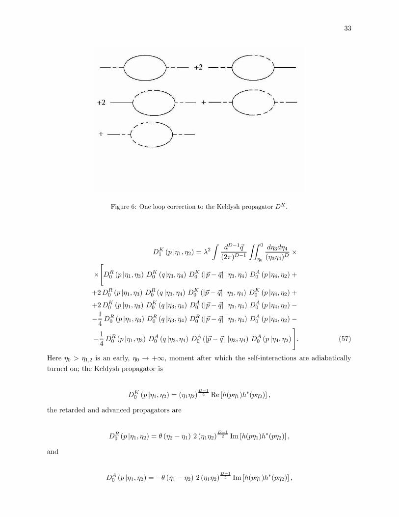
33
Figure 6: One loop correction to the Keldysh propagator DK .
DK1 (p |η1, η2) = λ2
∫
dD−1~q
(2π)D−1
∫∫ 0
η0
dη3dη4(η3η4)D
×
×[
DR0 (p |η1, η3) DK
0 (q|η3, η4) DK0 (|~p− ~q| |η3, η4) DA
0 (p |η4, η2) +
+2DR0 (p |η1, η3) DR
0 (q |η3, η4) DK0 (|~p− ~q| |η3, η4) DK
0 (p |η4, η2) ++2DK
0 (p |η1, η3) DK0 (q |η3, η4) DA
0 (|~p− ~q| |η3, η4) DA0 (p |η4, η2)−
−1
4DR
0 (p |η1, η3) DR0 (q |η3, η4) DR
0 (|~p− ~q| |η3, η4) DA0 (p |η4, η2)−
−1
4DR
0 (p |η1, η3) DA0 (q |η3, η4) DA
0 (|~p− ~q| |η3, η4) DA0 (p |η4, η2)
]
. (57)
Here η0 > η1,2 is an early, η0 → +∞, moment after which the self-interactions are adiabatically
turned on; the Keldysh propagator is
DK0 (p |η1, η2) = (η1η2)
D−12 Re [h(pη1)h
∗(pη2)] ,
the retarded and advanced propagators are
DR0 (p |η1, η2) = θ (η2 − η1) 2 (η1η2)
D−12 Im [h(pη1)h
∗(pη2)] ,
and
DA0 (p |η1, η2) = −θ (η1 − η2) 2 (η1η2)
D−12 Im [h(pη1)h
∗(pη2)] ,

34
correspondingly. Note that in these lectures we define Re [h1 h∗2] = h1 h
∗2 + h∗1 h2 and Im [h1 h
∗2] =
1i [h1 h
∗2 − h∗1 h2].
We will show below, that the leading IR contribution to DK1 (p |η1, η2) is hidden within the
following expression
DK1 (p |η1, η2) ≈ (η1 η2)
D−12
[
h(pη1)h∗(pη2)np(η) + h(pη1)h(pη2)κp(η) + c.c.
]
,
where np(η) ≈ − λ2
(2π)2(D−1)
∫
dD−1q1
∫
dD−1q2
∫∫ η
η0
dη3 dη4 (η3 η4)D−32 δ (~p+ ~q1 + ~q2)×
×h∗ (pη3) h (pη4) h∗(q1 η3)h(q1η4)h∗(q2η3)h(q2η4),
and κp(η) ≈2λ2
(2π)2(D−1)
∫
dD−1q1
∫
dD−1q2
∫ η
η0
dη3
∫ η3
η0
dη4 (η3 η4)D−32 δ (~p+ ~q1 + ~q2)×
×h∗ (pη3) h∗ (pη4) h∗(q1η3)h(q1η4)h∗(q2η3)h(q2η4). (58)
In deriving this expression from (57) we have used that in the IR limit in question one can neglect
the difference between η1 and η2 and substitute the average conformal time, η =√η1η2, instead of
both η1 and η2, in the upper limits of the integrations over η3 and η4. I.e., in (58) we dropped off
subleading terms of the order of λ2 log (η1/η2) or smaller, which may arise from integrals between
η1,2 and√η1η2.
Before performing the explicit calculation of (58) for the concrete choice of h(x), it is worth
checking what is happening in the flat space limit. To take this limit in (58) we just change η → t,
substitute η(D−1)/2 h(pη) by the plane wave, e−i ǫ(p) t/√
ǫ(p), and exchange√g = 1/ηD for one.
Then, as the upper limits of the time integrals in (58) go to future infinity, while the lower ones
are taken to past infinity, the time integrals are converted into the δ-functions establishing the
energy conservation: The integrands of∫∫
dq1 dq2 in the expressions for np and κp will contain the
time-line integrals of δ [ǫ(p) + ǫ(q1) + ǫ(q2)]. The argument of this δ-function is never zero. Hence,
the whole expressions for np and κp are vanishing.
Thus, we see that in the flat space limit the expressions for np and κp do vanish, which is the
consequence of the energy conservation. This gives us a hint for the physical interpretation of (58).
In fact, these expressions can arise in the presence of the particle creation process, when there
is no energy conservation due to the background gravitational field. Also this observation shows
that for the case of the EPP the contributions to np and κp from the past infinity, i.e., from the
region where pη ≫ µ and q1,2η ≫ µ, are negligible: When qη ≫ µ the function gp(η) can be well
approximated by the plane wave with the minor pre-exponential factor. Furthermore, this allows
one to safely take η0 to past infinity, η0 → +∞. In fact, dη3,4 integrals in (58) are converging in
the generalized sense on their lower limits of integration. The origin of these observations can be
traced back to the presence of the infinite blue shift towards the boundary between the EPP and
CPP.

35
1. Bunch–Davies vacuum
From now on we talk about the scalar fields from the principal series, m > (D − 1)/2, unless
otherwise stated. We comment on the complementary series in the last section.
So, we would like to estimate leading contributions to np and κp in (58) for the BD modes.
First, we take the integrals over ~q2 with the use of the δ-functions and rename ~q1 → ~q. Second, it
is straightforward to check that the largest IR contribution to (58) comes from the region where
q ≫ p inside the integral over dq. Hence, we neglect p in comparison with q under the integrals
in (58). That changes, however, the lower limits of integration over η3,4 from η0 → +∞ to µ/p.
Note that by doing this we just neglect the contributions to np and κp from the high energy region
pη3,4 ≫ µ.
Third, we make the following change of the integration variables in (58): q to x3 = qη3, η4 to
x4 = qη4 and leave η3 unchanged. As a result, the integration measure is converted into
∫∫∫
dq qD−2 dη3 dη4 (η3 η4)D−3
2 · · · =∫∫∫
dη3η3
dx3 dx4 (x3 x4)D−3
2 . . . .
Note that once the integral over q2 was taken and ~p was neglected in comparison with ~q ≡ ~q1, the
integrand of dD−1q depends only on |~q|.Now we can harmlessly extend the lower limits of integration over x3,4 to infinity both in np and
κp. Furthermore, in the expression for np we can extend the upper limits of integration over x3,4
to zero. In the expression for κp the latter change is done only for x3. These changes are harmless
because after them the integrals remain finite and pre-factors of the expressions, that we will find
below, are just slightly changed by the contributions from the high energy region.
Fourth, the integrals for np and κp are saturated around qη3,4 ∼ µ, while pη3,4 ≪ qη3,4. Hence,
we can expand
h(pη3,4) ≈ A+ (pη3,4)iµ +A− (pη3,4)
−iµ , where A± =
√π e±
πµ2
2±iµ+12 Γ (1± iµ) sinh (±πµ)
.
And finally, we perform the integration over η3 from µ/p to η and keep in the expressions for np
and κp only divergent, as pη → 0, terms. The result is
np(η) ≈λ2SD−2
(2π)D−1log
(
µ
p η
)∫∫ 0
∞dx3 dx4 (x3 x4)
D−32 ×
×[
|A+|2(
x4x3
)iµ
+ |A−|2(
x3x4
)iµ]
h2(x3) [h∗(x4)]
2 ,
κp(η) ≈ −2λ2SD−2
(2π)D−1log
(
µ
p η
)
A+A−
∫ 0
∞dx3
∫ x3
∞dx4 (x3 x4)
D−32 ×
×[
(
x4x3
)iµ
+
(
x3x4
)iµ]
h2(x4) [h∗(x3)]
2 , (59)
36
where SD−2 is the volume of the (D − 2)-dimensional sphere.
Once the initial state is the BD vacuum, the correlation function (58), (59) respects the dS
isometry. Hence, we are in a dS-homogenous stationary state and particle interpretation of our
formulas is not quite appropriate because 〈Tαβ〉 does not contain any fluxes6. In fact, the inverse
Fourier transformation of (58), with η-dependent np and κp from (59), will be a function of the
invariant geodesic distance between (η1, ~x1) and (η2, ~x2). One just has to bear in mind that in
(59) we have kept inside np and κp the leading contributions in the limit under consideration. I.e.,
we have forgot that in principle np and κp depend on η1 and η2 separately rather than on their
combination η =√η1η2.
However, to understand the physical meaning of the obtained expressions, let us for a moment
forget about the dS-invariance of (58), (59). That makes sense for the following reasons: At the
past infinity of the EPP np and κp have the clear interpretation as the particle density per comoving
volume, 〈a+p ap〉, and as the anomalous quantum average, 〈ap a−p〉, correspondingly. Then, if we
take some non-zero initial value of np, the dS isometry is broken even at tree level (by the initial
state). In fact, for non-zero, η-independent value of np (even when κp = 0) the inverse Fourier
transform ofDK(p|η1, η2) depends on each its time argument separately rather than on the invariant
geodesic distance. Moreover, below we will repeat the calculation in the situation when the dS
isometry is broken by an initial perturbation. The result will be the same as (58), but with a bit
different expressions for np and κp.
Thus, having in mind what we have just said, the physical interpretation of (58), (59) is as
follows. If we start from the vacuum, then both np and κp are zero at past infinity. As we have
seen above, in the absence of the gravitational field they also remain zero in future infinity. However,
once the gravitational field is turned on, they are generated in loops and are comparable to one,
even though they have been zero initially and λ2 is much less than one. So the presence of these
quantities signals the particle creation in the EPP. Moreover, below we give arguments favoring
that κp is the measure of the strength of the backreaction of quantum effects on the background
state. Hence, its significant presence signals that the backreaction on the initial BD state is strong,
i.e., in future infinity the system should relax to a different state from the BD one.
2. Contributions to the retarded and advanced propagators and to the vertices
Once we have understood the origin of the large IR corrections to the Keldysh propagator, let
us consider the situation in the case of the retarded (advanced) propagator and vertices. This will
be important for the summation of the leading IR corrections from all loops.
The one-loop diagram, that contributes to DR, is depicted on fig. 7. The corresponding
expression is:
6 It is interesting to note, however, that a free floating detector will click in such a stationary state. This is justa consequence of the fact that in the stationary state the Wightman function depends only on the hyperbolicdistance Z, which is equal to Z = cosh(τ1− τ2) if the spatial position of the detector is not changing. The detectorwill click because according to (33) the Wightman function has poles on the imaginary axis in the complex propertime-plain [65], [66].

37
Figure 7: One-loop correction to DR. For DA the diagram is mirror symmetric to this one.
Figure 8: Here we show some of the diagrams. The other diagrams are just complex conjugate of those that
are presented here.
DR1 (p |η1, η2) = λ2
∫
dD−1~q
(2π)D−1
∫∫ 0
+∞
dη3 dη4
(η3 η4)D
×
×DR0 (p |η1, η3) DR
0 (q |η3, η4) DK0 (|~q − ~p| |η3, η4) DR
0 (p|η4, η2) . (60)
Here one can immediately see that due to the presence of DR inside the loop and in the external
legs the limits of integration over η3,4 are such that η1 > η3 > η4 > η2. As a result, the loop integral
(60) does not receive large corrections in such a limit when η1/η2 is held fixed. In the different
limit, when say η1 → +∞ and η2 → 0, this integral can receive at most a correction proportional to
λ2 log (η1/η2) [71], but it is not of interest for us here. The situation with the advanced propagator
is the same.

38
The diagrams that contribute to the vertex renormalization are depicted on fig. 8. We find it
more convenient to consider loop contributions to vertices in the SK technique before the Keldysh
rotation (49). Then the expressions for these diagrams are as follows7:
λ−−−(η1,2,3; p1,2,3) = (−i λ)3 (η1 η2 η3)D−1
∫
dD−1p
(2π)D−1×
×[
θ(η1 − η2) h∗(pη1)h(pη2) + θ(η2 − η1) h∗(pη2)h(pη1)]
[
θ(η2 − η3) h∗ (|~p1 + ~p| η2) h (|~p1 + ~p| η3) + θ(η3 − η2) h∗ (|~p1 + ~p| η3) h (|~p1 + ~p| η2)]
[
θ(η3 − η1) h∗ (|~p2 − ~p| η3) h (|~p2 − ~p| η1) + θ(η1 − η3) h∗ (|~p2 − ~p| η1) h (|~p2 − ~p| η3)]
,
and λ+−−(η1,2,3; p1,2,3) = − (−i λ)3 (η1 η2 η3)D−1
∫
dD−1p
(2π)D−1×
×[
θ(η1 − η2) h∗(pη1)h(pη2) + θ(η2 − η1) h∗(pη2)h(pη1)]
h∗ (|~p1 + ~p| η2) h (|~p1 + ~p| η3) h (|~p2 − ~p| η3) h∗ (|~p2 − ~p| η1) , (61)
up to the factor of δ (~p1 + ~p2 + ~p3). Now it is straightforward to check that in the limit piηi → 0,
i = 1, 2, 3, there are no large IR contributions to these expressions. The fastest way to make this
observation is to put all the external momenta pi to zero and to see that, then, λ±±± are all finite.
At the same time, the one-loop correction to DK is divergent in this limit.
3. Other α-harmonics
Other α-modes can be relevant in the IR limit, although they show wrong behavior in the UV
limit. That is a quite frequent situation in condensed matter physics: One notable instance is the
BCS theory for superconductivity, where, to observe the Cooper pairing, one has to perform the
Bogolyubov rotation into harmonics, which, however, are inappropriate in the UV limit. Because
of that it is instructive to perform the one-loop calculation for them.
The leading IR contribution in this case also can be expressed in such a form as (58). For the
most values of α, both np and κp receive large contributions which are similar to (59), but with
different prefactors of log(pη). The only exception is given by the out-modes. In the latter case
h(x) ≈ Axiµ, as x→ 0, where A is some complex constant following from the proper normalization
of the harmonic functions and the expansion of the Bessel functions around zero.
To see the peculiarity of the out-modes and to calculate np and κp in this case, one has to
perform the same manipulations as have been done during the one-loop calculation for the BD
harmonics. However, if one substitutes the corresponding h(pη) into (58), he should take into
account that they behave at past infinity, x→ ∞, as follows
h(x) =1√x
[
A1 ei x +A2 e
−i x] , (62)
7 I would like to thank F.Popov and V.Slepukhin for the discussions on this point.
39
where A1,2 are some complex constants. Due to the interference terms between eix and e−ix, the
integrals over x3,4 do not converge fast enough: they are saturated in the vicinity of px3,4/q ∼ µ
rather than at x3,4 ∼ µ. (Note that according to our approximations p/q ≪ 1.) Hence, naively
one cannot Taylor expand h (px3,4/q) = h(pη3,4) around zero. However, if we are in D = 4, we
can subtract from and then add to h2(x), under these integrals, the value of the interference term,A1A2|x| :
h2(x) = h2(x)− A1A2
|x| +A1A2
|x| .
Then, the x3,4 integrals of h2(x) − A1 A2|x| are saturated around x3,4 ∼ µ and, hence, one can
Taylor expand h (px3,4/q) around zero inside the corresponding expressions. At the same time,
the contributions from the additional integrals of A1 A2|x| are suppressed in the IR limit. In fact,
due to extra powers of η3, the integrals over dη3 are not divergent in the limit as pη → 0. Thus,
performing these manipulations we fetch out the leading IR correction. In higher dimensions the
procedure is the same, but may demand a subtraction of higher powers of 1/|x|. It is interesting
to note that this kind of a problem does not appear in φ4 theory [58].
Thus, the contribution to the two-point function is as follows:
np(η) ≈λ2SD−2
(2π)D−1|A|2 log
(
µ
p η
)∫∫ 0
∞dx3 dx4 (x3 x4)
D−32
(
x4x3
)iµ
V (x3)V∗(x4),
where V (x) ≡ h2(x)− A1A2
|x| − . . . , (63)
and κp does not receive any large IR correction! As we will explain below, κp is the measure of the
backreaction strength. Hence, this observation is crucial for the proper quasi-particle interpretation
in future infinity.
D. One-loop correction in the contracting Poincare patch
Let us consider now one-loop corrections in the CPP. Similarly to the case of the EPP, it is not
hard to show that DR,A and vertices do not receive large IR corrections. At the same time, in the
limit pη0 → 0 the leading one-loop contribution to DK(p|η1, η2) can be written as (58). The crucial
difference, however, is that now 0 < η0 < η1,2 < +∞. Also one has to exchange the positive and
negative energy harmonics because of the time reversal.
To estimate the largest contribution to the integrals in np and κp, one has to perform the same
manipulations as we have been doing in the calculation on the EPP background. The results are
as follows. First, unlike the case of the EPP, now η0 cannot be taken to past infinity, η0 → 0.
Otherwise the integrals in np and κp will be explicitly divergent. Second, the answer for np and κp
depends on the value of pη = p√η1η2:
For the BD modes, which are out-harmonics in the CPP, the IR divergence is present both in
np and κp. If pη ≪ µ, it is proportional to log (η/η0) = τ − τ0. That is just the proper time elapsed

40
from η0 = eτ0 to η = eτ . If, however, pη ≫ µ, then the divergence is proportional to log (µ/pη0).
The coefficients of these divergences in both situations are the same as in (59).
For the Bessel or in-harmonics in the CPP, np(η) diverges as log (η/η0), if pη ≪ µ. At the same
time, when pη ≫ µ, the divergence in np is as log (µ/pη0). (The coefficients in both cases are the
same as in (63).) At the same time, in this case κp(η) does not have any divergence or large IR
contribution.
For any other type of α-harmonics the IR behavior of np and κp is similar to that of the BD
modes.
E. One-loop correction in global de Sitter space
We continue with the one-loop calculation in global dS. In this case the situation with the
retarded (advanced) propagator and with vertices is the same as in the EPP and CPP. Thus, we
consider here the Keldysh propagator. Following [56], we would like to show that in global dS space
the moment of turning on self-interactions cannot be taken to past infinity. Below we are going to
work with even dimensional dS spaces. In odd-dimensional global dS spaces the situation is a bit
different due to some cancelations [52], but in essential sense it is similar to the even-dimensional
case. The existence of the particle creation in the odd-dimensional case can be traced back to the
fact that also in odd dimensions it is not possible to diagonalize the corresponding free Hamiltonian
once and forever.
Unlike higher dimensional dS space, in the 2D case the one-loop calculation in global coordinates
can be made quite explicit. So let us present it before continuing with the IR divergences in general
dimensions. Again, due to spatial homogeneity of 2D global dS space together with background
states under consideration, we find it convenient to perform the Fourier transformation of all
quantities along the spatial direction ϕ ∈ [0, 2π]: DK,R,A(p|t1, t2) ≡∫ 2π0 dϕ ei p ϕDK,R,A(t1, ϕ; t2, 0).
Then, the one-loop contribution to DK is as follows:
DK1 (p|t1, t2) = λ2
+∞∑
q=−∞
∫∫ +∞
t0
dt3dt4 cosh(t3) cosh(t4)×
×[
DR0 (p|t1, t3)DK
0 (q|t3, t4)DK0 (|~p − ~q| |t3, t4)DA
0 (p|t4, t2) +
+2DR0 (p|t1, t3)DR
0 (q|t3, t4)DK0 (|~p− ~q| |t3, t4)DK
0 (p|t4, t2) ++2DK
0 (p|t1, t3)DK0 (q|t3, t4)DA
0 (|~p − ~q| |t3, t4)DA0 (p|t4, t2)−
−1
4DR
0 (p|t1, t3)DR0 (q|t3, t4)DR
0 (|~p − ~q| |t3, t4)DA0 (p|t4, t2)−
−1
4DR
0 (p|t1, t3)DA0 (q|t3, t4)DA
0 (|~p − ~q| |t3, t4)DA0 (p|t4, t2)
]
. (64)
Here the Keldysh propagator is
DK0 (p|t1, t2) = Re
[
gp(t1)g∗p(t2)
]
,

41
the retarded and advanced propagators are
DR0 (p|t1, t2) = θ (t1 − t2) 2 Im
[
gp(t1)g∗p(t2)
]
, and DA0 (p|t1, t2) = −θ (t2 − t1) 2 Im
[
gp(t1)g∗p(t2)
]
,
correspondingly; gp(t) is the temporal part of a solution of the KG equation, which we do not
specify for the beginning; t0 is the moment when self-interactions are turned on.
The above one-loop expression can be rewritten as:
DK1 (p|t1, t2) = −λ
2
2gp(t1) g
∗p(t2)
∑
q
∫∫ +∞
t0
dt3dt4 cosh(t3) cosh(t4)g∗p(t3) gp(t4)×
×
− θ(t1 − t3) θ(t2 − t4)
[
gq(t3) g∗q (t4) g|p−q|(t3) g
∗|p−q|(t4) + c.c.
]
+
[
θ(t1 − t3) θ(t3 − t4) + θ(t2 − t4) θ(t4 − t3)
][
gq(t3) g∗q (t4) g|p−q|(t3) g
∗|p−q|(t4)− c.c.
]
−
−λ2
2gp(t1) gp(t2)
∑
q
∫∫ +∞
t0
dt3dt4 cosh(t3) cosh(t4)g∗p(t3) g
∗p(t4)×
×
θ(t1 − t3) θ(t2 − t4)
[
gq(t3) g∗q (t4) g|p−q|(t3) g
∗|p−q|(t4) + c.c.
]
+
[
θ(t1 − t3) θ(t3 − t4)− θ(t2 − t4) θ(t4 − t3)
] [
gq(t3) g∗q (t4) g|p−q|(t3) g
∗|p−q|(t4)− c.c.
]
+ c.c. (65)
We need to find the leading contribution from this expression in the limit t ≡ t1+t22 → +∞,
t1 − t2 = const and t0 → −∞. (We take t0 → −∞ just to check if this limit is smooth.) As in the
case of the EPP and CPP, we can substitute t1,2 by t in the arguments of the θ-functions.
One can estimate directly the expression in Eq. (65). But instead of doing this we apply a
different procedure which allows us to find the leading corrections in any dimension. If t → +∞and t0 → −∞, then the leading IR contributions to DK
1 appear from the regions of integration over
t3,4 in the vicinity of t and t0. As we have explained above, in these regions the global dS metric
can be well approximated by those of the EPP and CPP. It is this observation which allows one to
estimate the one-loop correction in an arbitrary dimension. In fact, then gp(t) can be approximated
by
gp(t) ≈
ηD−1
2+ h+(pη+), η+ = e−t, t→ +∞η
D−12
− h−(pη−), η− = et, t→ −∞(66)
for non-zero p. (In an arbitrary dimension p coincides with the index of the temporal part of the
harmonics.) Then, as pη → 0 and pη0 → 0, where η = e−t and η0 = et0 , the leading IR contribution
to DK is hidden within [56], [62]:
42
DK1 (p|t1, t2) = gp(t1) g
∗p(t2)np(t) + gp(t1) gp(t2)κp(t) + c.c.,
where np(t) ≈ −λ2 SD−2
(2π)D−1
∫
dD−1q
∫∫ η
∞dη3 dη4 (η3 η4)
D−32 ×
×h∗+ (pη3) h+ (pη4) h∗+(q η3)h+(qη4)h
∗+ (|~q − ~p| η3) h+ (|~p− ~q| η4)−
−λ2 SD−2
(2π)D−1
∫
dD−1q
∫∫ ∞
η0
dη3 η4 (η3 η4)D−3
2 ×
×h∗− (pη3) h− (pη4) h∗−(qη3)h−(qη4)h
∗− (|~q − ~p| η3) h− (|~q − ~p| η4) ,
and κp(t) ≈2λ2 SD−2
(2π)D−1
∫
dD−1q
∫ η
∞dη3
∫ η3
∞dη4 (η3 η4)
D−32 ×
×h∗+ (pη3) h∗+ (pη4) h
∗+(qη3)h+(qη4)h
∗+ (|~q − ~p| η3) h+ (|~q − ~p| η4) +
+2λ2 SD−2
(2π)D−1
∫
dD−1q
∫ ∞
η0
dη3
∫ η3
η0
dη4 (η3 η4)D−3
2 ×
×h∗− (pη3) h∗− (pη4) h
∗−(qη3)h−(qη4)h
∗− (|~q − ~p| η3) h− (|~q − ~p| η4) . (67)
Thus, IR corrections in global dS space are just sums of the contributions from the contracting
(past infinity, i.e. around t0) and expanding (future infinity, i.e. around t) Poincare patches of the
whole space.
We continue with the description of the character of the IR divergences for different choices
of the α-modes. That may help to specify the convenient choice of the harmonics for the proper
definition of quasi–particles in the IR limit.
We start with the Euclidian harmonics. In this case, h∗−(x) = h+(x) ∝ H(1)iµ (x). Using that
h+(x) ≈ A+ xiµ + A− x−iµ, as x→ 0, and performing the same manipulations as in the EPP and
CPP, we obtain:
np(t) ≈λ2SD−2
(2π)D−1log
(
µ2
p2 η η0
)∫∫ ∞
0dx3 dx4 (x3 x4)
D−32 ×
×[
|A+|2(
x4x3
)iµ
+ |A−|2(
x3x4
)iµ]
h2(x3) [h∗(x4)]
2 ,
κp(t) ≈ −2λ2SD−2
(2π)D−1log
(
µ2
p2 η η0
)
A+A−
∫ 0
∞dx3
∫ x3
∞dx4 (x3 x4)
D−32 ×
×[
(
x4x3
)iµ
+
(
x3x4
)iµ]
h2(x4) [h∗(x3)]
2 . (68)
Note that to calculate the expression for κp we have used the identity A∗+A
∗− = A+A−. Thus,
for the Euclidian vacuum the leading IR divergence is proportional to log (1/ηη0) = (t− t0) and is
present both in np and κp.
At the same time, for the in-harmonics h−(x) is proportional to the Bessel function Yiµ(x).
Hence, h−(x) ≈ A∗ x−iµ, as x→ 0 (the past infinity of the CPP). But h+(x) ≈ C+ xiµ + C− x−iµ,
as x→ 0 (the future infinity of the EPP). Here C± are some complex constants related to A± via
the corresponding Bogolyubov α-rotation.

43
Then, the leading IR contribution in this case looks as:
np(t) ≈λ2SD−2
(2π)D−1log
(
µ
p η
)∫∫ 0
∞dx3 dx4 (x3 x4)
D−32 ×
×[
|C+|2(
x4x3
)iµ
+ |C−|2(
x3x4
)iµ]
V+(x3)V∗+(x4) +
+λ2SD−2
(2π)D−1log
(
µ
p η0
)∫∫ ∞
0dx3 dx4 (x3 x4)
D−32 |A|2
(
x4x3
)iµ
V ∗−(x3)V−(x4),
κp(t) ≈ −2λ2SD−2
(2π)D−1log
(
µ
p η
)
C∗+C
∗−
∫ 0
∞dx3
∫ x3
∞dx4 ×
× (x3 x4)D−32
[
(
x4x3
)iµ
+
(
x3x4
)iµ]
V+(x3)V∗+(x4). (69)
where V±(x) = h2±(x)− A1A2|x| − . . . and was defined above. (Dots here stand for the higher powers
of 1/|x|.) Note that for the in-harmonics np(t) depends separately on t and t0 rather than on their
difference (t− t0) and κp(t) does not diverge as t0 → −∞.
Similar conclusions are true for the out-harmonics. The crucial difference, however, is that in
the latter case κp does diverge as t0 → −∞, but is finite as t→ +∞. For the other α–harmonics the
leading IR contributions to np and κp also depend on t and t0 separately and diverge simultaneously
when t→ +∞ and t0 → −∞.
The presence of the IR divergence means that one cannot take the regulator, t0, to minus
infinity. Thus, one has to fix an initial Cauchy surface at some finite t0. (Such a surface does not
necessarily have to be taken somewhere around past infinity. One can put it, e.g., around the neck
of global dS space.) But holding t0 fixed, violates the dS-isometry.
V. SUMMATION OF LEADING INFRARED CONTRIBUTION IN ALL LOOPS
Thus, we see that λ2 log(η) and λ2 log(η0) contributions can become large, as η → 0 and η0 → 0,
even if λ2 is very small. I.e., loop corrections are not suppressed in comparison with classical tree
level contributions to the propagators. That is true even if the dS isometry is respected in loops.
Hence, to understand the physics in dS space, one has to sum unsuppressed IR corrections from
all loops.
We start with the discussion of the situation in the EPP and then continue with the CPP
and global dS space. In the EPP there is a separate interesting problem to sum dS-invariant IR
contributions to the correlation functions of the exact BD state (see, e.g., [87], [88]). As we pointed
out in the Introduction, solution of this problem is not sufficient to make a definite conclusion about
the stability of dS space: We find it as more physically sensible to question the stability of dS space
under nonsymmetric perturbations.
Hence, we propose to consider an initial nonsymmetric perturbation on top of the BD state.
But we cannot just put an initial comoving density at past infinity of the EPP, because then
the physical density will be infinite. One has to put the density perturbation at an initial Cauchy

44
surface which is different from the past infinity +∞ > η0 > 0. Moreover, due to the UV divergences
the comoving momentum also should be cutoff at the UV scale. But, as was explained above n(pη)
and κ(pη) are attributed to the comoving volume and, hence, do not change before pη ∼ µ.
Their behaviour for pη > µ is not much different from that in flat space–time. Thus, cutting
simultaneously comoving momentum and conformal time integrals effectively amounts to cut the
physical momentum integrals at µ. On the other hand, due to the symmetries of the EPP we can
put an initial comoving density at an initial value of the physical momentum (pη)0 ∼ ν and cutoff
all the integrals over the physical momentum at this value. Then, the dS isometry is broken by
the presence of a density on top of the dS-invariant BD state. (In the case of the CPP and global
dS space we do not even have to do this because the dS isometry is broken in loops for any initial
state.) We would like to trace the destiny of such a density perturbation and to understand the
effect of the large IR contributions on the initial state, as the system progresses towards future
infinity.
A. From the Dyson–Schwinger to the kinetic equation in the Poincare patches
To sum loop contributions one has to solve the system of Dyson-Schwinger (DS) equations
for the propagators, self-energies and vertices. We would like to sum only powers of the leading
contribution, λ2 log(pη), and neglect suppressed terms, such as, e.g., λ4 log(pη) or λ2 log(η1/η2)
and etc.. As we have seen above, the retarded and advanced propagators do not receive large IR
contributions from the first loop. The same is true for the vertices. However, these quantities may
receive large contributions from the second or higher loops. In fact, the latter may come from those
corrections to the Keldysh propagator which appear at lower loops. But this just means that such
contributions to DR,A and vertices will be suppressed by higher powers of λ. Thus, if we need to
perform only the summation of the leading corrections, then we have to care only about the DS
equation for the Keldysh propagator.
In the following, we assume that DR,A and vertices take their tree level values (perhaps renor-
malized by the UV contributions) and assume that all IR corrections go into IR exact DK . Then,
the relevant DS equation acquires the form:
DK(p|η1, η2) = DK0 (p|η1, η2) +
+λ2∫
dD−1~q
(2π)D−1
∫∫ 0
∞
dη3dη4(η3η4)D
[
DR0 (p|η1, η3)DK(q|η3, η4)DK(|~p − ~q| |η3, η4)DA
0 (p |η4, η2) +
+2DR0 (p|η1, η3)DR
0 (q|η3, η4)DK(|~p− ~q| |η3, η4)DK(p|η4, η2) ++2DK(p|η1, η3)DK(qη3, η4)D
A0 (|~p − ~q| |η3, η4)DA
0 (p|η4, η2)−
−1
4DR
0 (p|η1, η3)DR0 (q|η3, η4)DR
0 (|~p − ~q| |η3, η4)DA0 (p|η4, η2)−
−1
4DR
0 (p|η1, η3)DA0 (q|η3, η4)DA
0 (|~p − ~q| |η3, η4)DA0 (p|η4, η2)
]
, (70)
where DK0 (p|η1, η2) is the initial (tree level) value of the propagator. We propose the following

45
ansatz to solve this equation:
DK(p|η1, η2) = (η1η2)D−1
2 dK(pη1, pη2), where
dK(
pη1, pη2)
=1
2h(
pη1)
h∗(
pη2)
[
1 + 2np(
η)
]
+ h(
pη1)
h(
pη2)
κp(
η)
+ c.c.. (71)
Here η =√η1η2, np(η) and κp(η) are unknown functions to be defined by the equations under
derivation. Below we also use the notation d−(pη1, pη2) = 2 Im [h(pη1)h∗(pη2)] to simplify the
equations. The ansatz for the IR exact Keldysh propagator is inspired by the one-loop calculation
and its physical interpretation.
For general values of η1 and η2 the ansatz (71) does not solve (70). However, in the limit
pη1,2 → 0 and η1/η2 = const one can neglect the difference between η1 and η2 in the expressions
that follow and substitute the average conformal time η =√η1η2 instead of both η1 and η2 for the
limits of integrations over η3 and η4. Then, the ansatz in question solves the DS equation if np
and κp obey:
np(η) ≈ n(0)p − λ2∫
dD−1q
(2π)D−1
∫∫ η
∞dη3 dη4 (η3η4)
D−32 ×
×[
dK(
qη3, qη4
)
dK(
|~p− ~q| η3, |~p− ~q| η4)
+1
4d−(
qη3, qη4
)
d−(
|~p− ~q| η3, |~p− ~q| η4)
−
−d−(
qη3, qη4
)
dK(
|~p− ~q| η3, |~p− ~q| η4)[
1 + 2n(
pη13)
]
]
h∗(
pη3)
h(
pη4)
+
+4 θ (η4 − η3) dK
(
|~p− ~q| η3, |~p− ~q| η4)
Re
[
d−(
qη3, qη4
)
h(
pη3)
h(
pη4)
κ(
pη42)
]
(72)
and
κp(η) ≈ κ(0)p − λ2∫
dD−1q
(2π)D−1
∫∫ η
∞dη3 dη4 (η3η4)
D−32 ×
×[
dK(
qη3, qη4
)
dK(
|~p− ~q| η3, |~p− ~q| η4)
+1
4d−(
qη3, qη4
)
d−(
|~p− ~q| η3, |~p− ~q| η4)
+
+d−(
qη3, qη4
)
dK(
|~p− ~q| η3, |~p− ~q| η4)[
1 + 2n(
pη13)
]
]
h∗(
pη3)
h∗(
pη4)
+
+4 θ (η4 − η3) dK
(
|~p− ~q| η3, |~p− ~q| η4)
d−(
qη3, qη4
)
h∗(
pη3)
h(
pη4)
κ(
pη42)
(73)
where n(0)p and κ
(0)p define the initial propagator DK
0 (p|η1, η2) via Eq. (71).
In the derivation of (72) and (73) we have used the following relations d−(pη1, pη2) =
−d−(pη2, pη1) = −[
d−(pη1, pη2)
]∗and
∫
dD−1~qf (q, |~p− ~q|) =∫
dD−1~qf (|~p− ~q| , q). Below we
assume that np(η) and κp(η) are slow functions in comparison with h(pη). Then, one can safely
change arguments of all n’s and κ’s to the external time η. This is possible because of the usual

46
separation of scales, which lays in the basis of the kinetic theory [59]. In our case this approx-
imation is correct at least for the fields from the principal series, m > (D − 1)/2, because their
harmonics h(pη) oscillate at future infinity.
Note that for the scalars from the complementary series, m ≤ (D − 1)/2 the ansatz (71) also
solves (70). But in this case harmonics do not oscillate at future infinity and, hence, can be as
slow as np and κp. The main problem with the situation when h(pη) is slow function is that then
one cannot derive the kinetic equation of the usual form. More complicated integrodifferential
equations are available whose solution and physical interpretation is not yet known to us.
To avoid such a situation when the equations themselves depend on their initial data, we would
like to convert the integral equations (72), (73) into their integrodifferential form, i.e., into the
form of the kinetic equation [59]. This is done via a kind of the renormalization group procedure
as follows [61], [62], [58]. In the given settings, n(0)p and κ
(0)p are the particle density and anomalous
average at some moment after η∗ ∼ µ/p. In fact, as we will explain below, before this moment,
all the kinetic processes in the theory under consideration are suppressed because of the strong
blue shift. Hence, before η∗ ∼ µ/p, np(η) and κp(η) remain practically unchanged, i.e. can
be set equal to their initial values, n(0)p and κ
(0)p , correspondingly. Then, from (72), (73) it is
straightforward to find that due to the large IR corrections the difference between np(η), κp(η) and
n(0)p = np(η∗), κ
(0)p = κp(η∗) is proportional to the proper time elapsed from η∗ to η. Also one can
approximate:
np(η)− np(η∗)
log(η)− log(η∗)→ dnp(η)
d log(pη), and
κp(η)− κp(η∗)
log(η)− log(η∗)→ dκp(η)
d log(pη).
The coefficients of the proportionality between the elapsed time and the change of np and κp are
the so-called collision integrals. With the use of the following matrixes:
Np(η1, η2) = ηD−1
22
(
np(η1)h∗(pη2) κp(η1)h(pη2)
κp(η1)h(pη2) np(η1)h∗(pη2)
)
, P =
(
0 1
1 0
)
(74)
the collision integrals for np and κp can be written compactly. The real one for np has the form:
dnp(η)
d log(pη)= 2λ2
∫
dD−1q
(2π)(D−1)
∫ ∞
0
η dη′
(η η′)DRe Tr
Cp,q,p−q(η)
[
(
1 +N∗p
)
NqNp−q − N∗p (1 +Nq) (1 +Np−q)
]
(η, η′)+
+2Cq,q−p,p(η)[
N∗q (1 +Nq−p) (1 +Np) −
(
1 +N∗q
)
Nq−pNp
]
(η, η′) +
+Dp,q,p+q(η)[
(1 +Np) (1 +Nq) (1 +Np+q) − NpNqNp+q
]
(η, η′)
+ [N → P N ] . (75)
At the same time the complex collision integral for κp is as follows:

47
dκp(η)
d log(pη)= −2λ2
∫
dD−1q
(2π)(D−1)
∫ η
0
η dη′
(η η′)D(~p→ −~p) Tr
Cp,q,p−q(η)[
(1 +Np) (1 +Nq) (1 +Np−q) − NpNq Np−q]
(η, η′)+
+2C∗q,q−p,p(η)
[
N∗q (1 +Nq−p) (1 +Np) −
(
1 +N∗q
)
Nq−pNp
]
(η, η′) +
+D∗p,q,p+q(η)
[
(1 +Np) N∗q N
∗p+q − Np
(
1 +N∗q
) (
1 +N∗p+q
)
]
(η, η′)
− [N → P N ] . (76)
The term [N → P N ] means that we have to add to the explicitly written expressions in (75) and
(76) the same quantities with every N substituted by the product P N ; Re Tr means that one
has to take the real part and the trace of the expression that stands after this sign; (~p→ −~p) Trmeans that one has to take the trace and add to the expression standing after this sign the
same term with the exchange ~p → −~p. Finally, to simplify the equations we use the notations:
Ck1k2k3(η) = η3 (D−1)
2 h∗(k1η)h(k2η)h(k3η) and Dk1k2k3(η) = η3(D−1)
2 h(k1η)h(k2η)h(k3η).
Similarly to Eq. (58), the system of equations (75), (76) represents just a preliminary version
of the kinetic equations. It is not yet suitable to sum only the leading IR contributions in all loops
because on top of the latter it also accounts for some of the subleading corrections. In particular,
one should restrict the dq integrals in (75) and (76) to the region q ≫ p and Taylor expand h(pη)
and h(pη′) around zero. As we discussed above, it is this region where the leading IR contributions
come from.
1. Physical meaning of infrared effects
Before going further let us explain the meaning of the system of equations (75) and (76). To do
that let us forget for the moment about the presence of κp and consider the situation in flat space.
If the time of the turning on self-interactions is t0 and the time of the observation is t, then the
kinetic equation is:
dnpdt
∝ −λ2∫
dD−1q
ǫ(p) ǫ(q) ǫ(p − q)×
∫ t
t0
dt′ cos[
(−ǫ(p) + ǫ(q) + ǫ(p− q)) (t− t′)]
[
(1 + np)nq n|p−q| − np (1 + nq) (1 + n|p−q|)
]
(t)
+2
∫ t
t0
dt′ cos[
(−ǫ(q) + ǫ(q − p) + ǫ(p)) (t− t′)]
[
nq (1 + n|q−p|) (1 + np) − (1 + nq)n|q−p| np]
(t)
+
∫ t
t0
dt′ cos[
(ǫ(q) + ǫ(q + p) + ǫ(p)) (t− t′)]
[
(1 + nq) (1 + nq+p) (1 + np) − nq nq+p np
]
(t)
,(77)
where ǫ(p) is the energy of the particle with the momentum ~p. There are many ways to derive this
kinetic equation (see, e.g., appendix of [57]). One of them is similar to that method which was
presented above for dS space.
In the limit (t−t0) → ∞ the dt′ integrals in (77) are converted into (minus) δ-functions ensuring
energy conservation in some processes, which we will define now. The expression in the second line

48
of Eq. (77), which is multiplying dt′ integral, describes the competition between the following two
processes. One of them corresponds to the term np (1 + nq) (1 + n|p−q|) and is such a process in
which a particle with momentum ~p decays into two excitations — ~q and ~p− ~q. This term appears
with the minus sign in the collision integral because it describes the loss of an excitation with
the momentum ~p. The inverse gain process, corresponding to the term (1 + np)nq n|p−q| with the
plus sign, is such that two particles, ~q and ~p− ~q, are merged together to create an excitation with
momentum ~p.
The third line in (77) also describes two competing processes. The first of them is such that
a particle with momentum ~p joins together with another one, ~q − ~p, to create an excitation with
momentum ~q. This is the loss process. The inverse gain process is the one in which a particle with
momentum ~q decays into two, one of which is with momentum ~p. The coefficient 2 in front of this
term is just the combinatoric factor.
Similarly the fourth line describes two processes. The gain process is when three particles, one
of which is with momentum ~p, are created by an external field, if any. The loss process is when
three such excitations are annihilated into vacuum.
All these six types of processes are not allowed by the energy–momentum conservation for
massive fields with φ3 self-interaction in flat space-time8. Hence, the collision integral is vanishing
as (t − t0) → ∞. However, in dS space these processes are allowed [72]–[86] because there is no
energy conservation.
One can obtain from (77) the collision integral of Eq. (75) with κp set to zero. To do that
it is necessary to exchanges dt′ for dη′, multiply it by the proper weight,√g, following from
the nontrivial metric, and to use the dS harmonics, gp(η) = ηD−1
2 h(pη), instead of the plane
waves, e−i ǫ(p) t/√
ǫ(p). Then, instead of the above mentioned δ-functions, which ensure energy
conservation, there are some expressions, which define the differential rates (per given range of ~q)
of the processes described in the above three paragraphs.
Note that in the free theory (λ = 0) np remains constant. This is an indirect argument favoring
that np is the particle density per comoving volume. (The direct argument follows from the
calculation of the density from the Wightman function.) Furthermore, due to the presence of κp,
in (75) we have extra terms on top of those which are shown in (77). All of them can be obtained
from (77) via the simultaneous substitutions of some of (1+nk)’s and nk’s by κk’s or κ∗k’s. E.g. in
(75) we encounter terms of the type:
[
(1 + np)κp n|p−q| − np κq (1 + n|p−q|)]
. (78)
The meaning of (78) is that it describes the following two competing processes — a particle with
momentum ~p is lost (gained) in such a situation, in which instead of the creation (annihilation) of
two particles, with momenta ~q and ~p−~q, we obtain a single excitation ~p−~q and missing momentum
~q is gone into (taken from) the background quantum state of the theory.
8 For the massless flat space φ3 theory the collision integral in (77) is not zero. The second and the third lines in(77) describe nontrivial decay processes for the collinear momenta of the products of the reactions. In this case(77) will describe, e.g., phonons in solid bodies if instead of the speed of light one would use that of sound.

49
Similarly we encounter terms of the type
[
(1 + np)κq κ|p−q| − np κq κ|p−q|]
(79)
which describe the processes in which both momenta ~q and ~p − ~q are coming from (going to) the
background state. These observations, in particular, justify the interpretation of κp as the measure
of the strength of the backreaction on the background state of the theory.
Now put both np and κp to zero inside collision integral (75). The only term which survives
then is present in the last line of (75) or (77). It describes the particle creation process by the dS
gravitational field. If one takes the integral of this term over the conformal time from η0 to η he
obtains exactly the expression for np(η) from (58). Using the collision integral for κp, (76), one
can make similar observation about the origin of the corresponding expression in (58).
Thus, in the nonstationary situations, i.e., when the collision integral is not zero, it is natural to
expect a linear time-divergence, ∝ (t− t0), in np and κp. That indeed is true for the homogeneous
in time background fields (such as, e.g., constant electric fields in QED), when particle production
rates are constant. But, in the time dependent metric of dS space one encounters a bit different
situation. In particular, in the EPP the largest IR contributions have the form of λ2 log (µ/pη) and
there is no IR divergence as one takes the moment of turning on self-interactions to past infinity,
η0 → +∞. That happens because the creation of particles with comoving momentum p effectively
starts at η∗ ∼ µ/p rather than at the moment when we turn on self-interactions, η0 → +∞. For
the same reason in the CPP the particle creation process goes on until η∗ ∼ µ/p and then stops,
as we have seen from the one-loop calculation.
We encounter such a situation because, first of all, the collision integral is not just a constant
and depends on time. Second, the past (future) infinity of the EPP (CPP) corresponds to the
UV limit of the physical momentum. In this limit gp(η) harmonics behave as plane waves. As a
result, all the rates inside the collision integral can be well approximated by δ-functions ensuring
energy conservation [57], [61], [62]. Hence, the collision integral becomes negligible as pη → ∞both in the EPP and CPP. That is the reason why in the EPP, independently of the type of the
harmonics, one can put the moment of turning on self-interactions, η0, to past infinity. Similarly
these observations explain the time-independence of the leading IR contributions in the CPP, when
η > µ/p.
2. The kinetic equation
The DS equation (70) is covariant under the simultaneous Bogolyubov rotation of the harmonics
and of np and κp. Hence, in principle a solution of (70) in terms of one type of harmonics can be
mapped to another type.
However, we would like to choose such harmonics, h(pη), for which there is a solution of (75),
(76) with κp being zero. From the one-loop calculations it is not hard to find that most of α-modes,
including the BD ones, do not provide such a solution. That means that the backreaction on the
corresponding ground states is strong. Only for the out-harmonics, h(x) ∝ Jiµ(x), the situation is

50
different. In particular, if one puts κp(η) to zero it is not generated back in (72), (73). Or more
precisely, contribution to it behaves as λ2, i.e., is negligible in comparison with λ2 log(pη).
All in all, out-harmonics represent the proper quasi-particle states in future infinity. Which
means that for out-modes the ansatz (71) solves the DS equation with κp(η) ≡ 0. This is the
argument which favors the interpretation that independently of the initial state at the past infinity
of the EPP the field theory state flows in future infinity to the out-vacuum with some density of
particles on top of it [57]. To support such a conclusion, we will show in a moment that for the
out-harmonics κp(η) indeed flows to zero in future infinity, even if originally it had some small
non-zero value.
The kinetic equation for out-modes is obtained from (72), (73), with κp(η) set to zero, via the
same “renormalization group” procedure as was used above. The result is:
dn(x)
d log(x)= −λ
2 SD−2 |A|2(2π)D−1
∫ 0
∞dx3 x
D−32
3
∫ 0
∞dx4 x
D−32
4 ×
×
Re[
x−iµ3 V (x3)xiµ4 V ∗(x4)
]
[1 + n(x)]n(x3)2 − n(x) [1 + n(x3)]
2
+
+2Re[
xiµ3 W (x3)x−iµ4 W (x4)
]
n(x3) [1 + n(x3)] [1 + n(x)] − [1 + n(x3)]n(x3)n(x)
+
+ Re[
xiµ3 V (x3)x−iµ4 V ∗(x4)
]
[1 + n(x3)]2 [1 + n(x)] − n(x3)
2 n(x)
, (80)
where x = pη, V (x) =[
h2 (x)− A1 A2|x| − . . .
]
, W (x) =[
|h (x)|2 − A1A2|x| − . . .
]
and h(x) =√
πsinh(πµ) Jiµ(x). We have done here the same approximations as in the one-loop calculation.
Now we have to check the stability of (80) under the linearized perturbations of κp(η). If one
keeps only the linear in κp terms, the integrodifferential form of the equation, which follows from
(73), degenerates to:
dκp(η)
d log(pη)= Γ3 κp(η),
Γ3 =4 i λ2 SD−2 |A|2
(2π)D−1
∫∫ 0
∞dx3 dx4 x
D−32
−iµ3 x
D−32
+iµ
4 θ(x4 − x3) Im [V (x3)V∗(x4)] . (81)
Below we will show that ReΓ3 > 0 and, hence, the solution of this equation, κp(η) ∝ (pη)Γ3 ,
reduces back to zero, as η → 0.
B. Solution of the kinetic equation in the Poincare patches
To find a solution of the kinetic equation (80) it is instructive to consider simultaneously the
situation in the EPP and CPP. Spatially homogeneous kinetic equations in EPP and CPP can
be trivially related to each other, because to perform the map from EPP to CPP one just has
to flip the limits of dη′ integration inside the collision integrals in (75) and (76). On top of that
it is necessary to make the change of h(x) to h∗(x), because the positive energy harmonics are

51
exchanged with the negative ones under the flip of the time direction. As a result, solutions in
both patches also can be mapped to each other. That is physically meaningful because the system
of kinetic equations (75) and (76) is valid for the spatially homogeneous states and is imposed on
the quantities which are attributed to the comoving volume. It is worth mentioning that spatially
homogenous situation in the CPP is unstable under small inhomogeneous density perturbations.
However, it is still instructive to consider such an ideal situation in the CPP9.
Thus, all the observations made for the EPP can be extended to the CPP. For the Bessel
(in-)harmonics in the CPP the corresponding system (75) and (76) can be reduced to the single
equation:
dnp(η)
d log (η/η0)=λ2 SD−2 |A|2(2π)D−1
∫ ∞
0dq η (qη)
D−12
∫ ∞
0dη′ q
(
qη′)
D−12 ×
×
Re[
(qη)−iµ V (qη)(
qη′)iµ
V ∗(qη′)]
[1 + np]n2q − np [1 + nq]
2
(η) +
+2Re[
(qη)iµW (qη)(
qη′)−iµ
W (qη′)]
nq [1 + nq] [1 + np] − [1 + nq]nq np
(η) +
+Re[
(qη)iµ V (qη)(
qη′)−iµ
V ∗(qη′)]
[1 + nq]2 [1 + np] − n2q np
(η)
. (82)
Neither (80) nor (82) possess the Plankian distribution as a stationary solution, because there is no
energy conservation. However, one can find a distribution which annihilates the collision integral
of (80) or (82) in a different manner: while Plankian distribution in ordinary kinetic equation
annihilates each term, describing aforementioned couples of competing processes, separately, in
the present case we will see the cancelation between different terms. The situation is somewhat
similar to the one in which appears the turbulent stationary Kolmogorov like scaling. That is
natural to expect in a system with energy pumping in at one scale and its loss at another one.
Thus, suppose we have started at the past infinity of the EPP with some very mild density
perturbation over the BD state. After the Bogolyubov rotation to the out-harmonics, one has
some initial values of np and κp. As can be understood from the discussion above, for the given
p, the density np and the anomalous average κp practically do not change before η∗ ∼ µ/p. After
this moment they begin to evolve according to (75), (76). If κp is sufficiently small, it relaxes to
zero, as we have shown above, and the problem is reduced to the solution of (80).
Now, if the initial value of np after the rotation to the out-harmonics is much smaller than one,
we can use the following approximations:
[1 + n(x)]n(x3)2 − n(x) [1 + n(x3)]
2 ≈ −n(x),n(x3) [1 + n(x3)] [1 + n(x)]− [1 + n(x3)]n(x3)n(x) ≈ n(x3),
9 Actually it is not very hard to find the inhomogeneous extension of the kinetic equation (80). In the case in whichthe particle density starts to depend also on the spatial position np = np(η, ~x), one has to substitute η d/dη by
η ∂η + η2~p ~∂x on the left hand side of (80). The extra η2~p~∂x term is the simplest expression that is invariant underthe symmetries of the EPP and CPP metrics: such as, e.g., simultaneous scaling of all coordinates.

52
[1 + n(x3)]2 [1 + n(x)]− n(x3)
2 n(x) ≈ 1. (83)
Because of the rapid oscillations of h(x) as x→ ∞, the integrals on the right hand side of (80) are
saturated at x3,4 ∼ µ. At the same time pη ≪ µ and it is natural to assume that n(x3,4 ∼ 1) ≪n(pη) in the situation of the very small initial density perturbation and the vanishing production
of the high momentum modes. Hence, we can neglect the second contribution (∼ n(x3)) on the
right hand side of (80), (83) in comparison with the first (∼ n(x)) and the third (∼ 1) ones.
As a result, Eq. (80) is reduced to
dn(x)
d log(x)≈ Γ1 n(x)− Γ2,
Γ1 =λ2 SD−2 |A|2(2π)D−1
∣
∣
∣
∣
∫ ∞
0dy y
D−32
−i µ[
h2 (y)− A1A2
|y|
]∣
∣
∣
∣
2
,
Γ2 =λ2 SD−2 |A|2(2π)D−1
∣
∣
∣
∣
∫ ∞
0dy y
D−32
+i µ
[
h2 (y)− A1A2
|y|
]∣
∣
∣
∣
2
(84)
Here, Γ1 and Γ2 are the particle decay and production rates, correspondingly. Note that x = pη is
reducing to zero during the evolution towards the future infinity.
The obtained equation (84) has the solution with the flat stationary point distribution n(pη) =
Γ2/Γ1, which corresponds to the situation in which the production (gain) of particles on the level
pη is equilibrated by the particle decay (loss) from the same level. The obtained solution is self-
consistent for the large enough µ because then Γ2/Γ1 ≈ e−2 πµ ≪ 1, which is not hard to show
using the following property of the Hankel functions:
∫ ∞
0dxx
D−32
+iµ(
H(1)iµ (x)
)2= e−2πµ
∫ ∞
0dxx
D−32
−iµ(
H(2)iµ (x)
)2. (85)
(Also it is not hard to show that the introduced in the previous subsection Γ3 obeys ReΓ3 =
Γ1 − Γ2 ≈(
1− e−2πµ)
Γ1 > 0.)
So the result of the summation of the large IR contributions may lead to the well behaving exact
two-point function. As a result, the dS isometry, which was broken by the initial perturbation, is
asymptotically restored at future infinity. But what if the evolution had started with some quite
strong density perturbation (which is, however, still much smaller than the vacuum energy) over
the BD vacuum state? Now, we are going to show that there is another very peculiar solution of
the kinetic equation under consideration.
Suppose that, due to the particle self-reproduction, the density per comoving volume on the
given level with pη ≪ µ became big in comparison with one. Taking into account the flatness of the
spectrum in dS space, it is natural to expect that, for the harmonics with the low physical momenta,
the density very slowly depends on its argument. Hence, we can assume that n(pη) ≈ n(qη) when
both pη ≪ µ and qη ≪ µ.
Then, we can make the following approximations:

53
[1 + n(pη)]n2(x3)− n(pη) [1 + n(x3)]2 ≈ −n2(pη),
n(x3) [1 + n(x3)] [1 + n(pη)]− [1 + n(x3)]n(x3)n(pη) ≈ n2(pη),
[1 + n(x3)]2 [1 + n(pη)]− n(x3)n(pη) ≈ n2(pη) (86)
and accept that, on the right hand side of (80), the main contribution to the x3,4 integrals comes
form the region in which x3,4 ≪ µ because n(x) ≫ n(y) if x ≪ µ and y ≫ µ. As a result, the
kinetic equation reduces to
dnp(η)
d log(η)= Γn2p(η), where
Γ ≈ λ2
(2π)D−1 µ3
∫ µ
0dy (y)
D−32
−Re
[
y−i µ∫ µ
0dy′ (y′)
D−32
+i µ
]
+
+2Re
[
y−i µ∫ µ
0dy′ (y′)
D−32
+i µ
]
+
+ 3Re
[
y−3 i µ
∫ µ
0dy′ (y′)
D−32
+3 i µ
]
> 0. (87)
Note that Γ is independent of p. This equation has the following solution:
np(η) ≈1
Γ log (η/η⋆), (88)
where η⋆ = µp e
−CΓ and C is an integration constant, which depends on initial conditions. The
obtained solution is valid if µ/p = η∗ > η > η⋆.
Thus, we see that there is a singular solution of the kinetic equation under consideration,
which corresponds to the explosion of the particle number density per comoving volume within a
finite proper time. Of course, such an explosion wins against the expansion of the EPP because
DK ∝ ηD−1
log η/η⋆. Hence, there are contributions to the energy-momentum tensor of the created
particles which become huge, and the backreaction has to be taken into account. As a result, the
dS space gets modified. But that is the problem for a separate study. At this point, we just would
like to stress that we see catastrophic IR effects even for the massive fields. It is natural to expect
that, for the light fields, the situation will be even more dramatic.
In the CPP, we can find similar solutions of the kinetic equation (82). For example, (84) is
mapped to
dnp(η)
d log(η/η0)≈ −Γ1 np(η) + Γ2, (89)
which shows a very peculiar phenomenon that, although in the first loop η0 cannot be taken to
the past infinity, after the summation of all loops, we can find the theory at the stationary point
state, np = Γ2/Γ1, which allows one to remove the IR cutoff, η0, and restore the dS isometry.
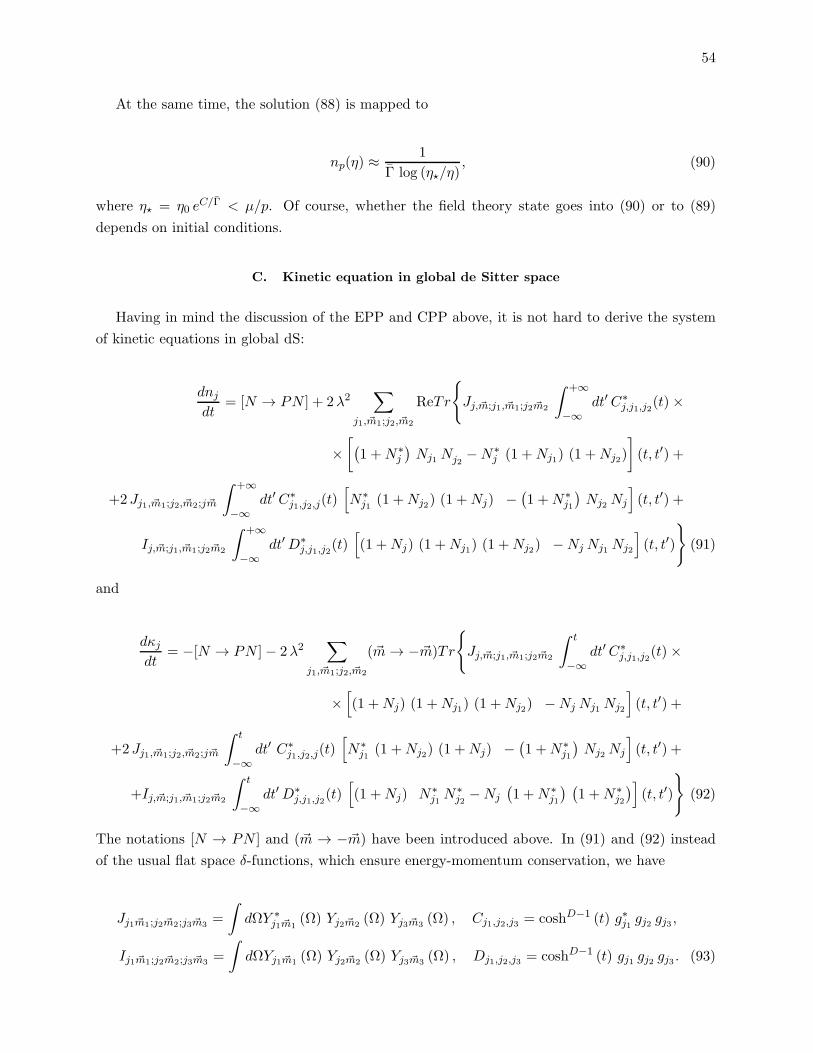
54
At the same time, the solution (88) is mapped to
np(η) ≈1
Γ log (η⋆/η), (90)
where η⋆ = η0 eC/Γ < µ/p. Of course, whether the field theory state goes into (90) or to (89)
depends on initial conditions.
C. Kinetic equation in global de Sitter space
Having in mind the discussion of the EPP and CPP above, it is not hard to derive the system
of kinetic equations in global dS:
dnjdt
= [N → PN ] + 2λ2∑
j1, ~m1;j2, ~m2
ReTr
Jj,~m;j1, ~m1;j2 ~m2
∫ +∞
−∞dt′ C∗
j,j1,j2(t)×
×[
(
1 +N∗j
)
Nj1 Nj2−N∗
j (1 +Nj1) (1 +Nj2)
]
(t, t′) +
+2Jj1, ~m1;j2, ~m2;j ~m
∫ +∞
−∞dt′C∗
j1,j2,j(t)[
N∗j1 (1 +Nj2) (1 +Nj) −
(
1 +N∗j1
)
Nj2 Nj
]
(t, t′) +
Ij,~m;j1, ~m1;j2 ~m2
∫ +∞
−∞dt′D∗
j,j1,j2(t)[
(1 +Nj) (1 +Nj1) (1 +Nj2) −Nj Nj1 Nj2
]
(t, t′)
(91)
and
dκjdt
= −[N → PN ]− 2λ2∑
j1, ~m1;j2, ~m2
(~m→ −~m)Tr
Jj,~m;j1, ~m1;j2 ~m2
∫ t
−∞dt′C∗
j,j1,j2(t)×
×[
(1 +Nj) (1 +Nj1) (1 +Nj2) −Nj Nj1 Nj2
]
(t, t′) +
+2Jj1, ~m1;j2, ~m2;j ~m
∫ t
−∞dt′ C∗
j1,j2,j(t)[
N∗j1 (1 +Nj2) (1 +Nj) −
(
1 +N∗j1
)
Nj2 Nj
]
(t, t′) +
+Ij,~m;j1, ~m1;j2 ~m2
∫ t
−∞dt′D∗
j,j1,j2(t)[
(1 +Nj) N∗j1 N
∗j2 −Nj
(
1 +N∗j1
) (
1 +N∗j2
)
]
(t, t′)
(92)
The notations [N → PN ] and (~m → −~m) have been introduced above. In (91) and (92) instead
of the usual flat space δ-functions, which ensure energy-momentum conservation, we have
Jj1 ~m1;j2 ~m2;j3 ~m3=
∫
dΩY ∗j1 ~m1
(Ω) Yj2 ~m2(Ω) Yj3 ~m3
(Ω) , Cj1,j2,j3 = coshD−1 (t) g∗j1 gj2 gj3 ,
Ij1 ~m1;j2 ~m2;j3 ~m3=
∫
dΩYj1 ~m1(Ω) Yj2 ~m2
(Ω) Yj3 ~m3(Ω) , Dj1,j2,j3 = coshD−1 (t) gj1 gj2 gj3 . (93)

55
Unlike the case of EPP and CPP, we do not yet understand what is the appropriate choice of the
harmonics for this system of kinetic equations. In fact, if one considers the entire dS space, then
κp is divergent either when t0 → −∞ or when t→ ∞, or in both cases simultaneously. In this case
none of the harmonics provides a proper quasi-particle description. However, if one will consider
that half of global dS space, which is above its neck, then the situation would be similar to that in
the EPP. I.e., in this case one can find the same solutions as we have found above.
VI. SKETCH OF THE RESULTS FOR λφ4 THEORY (INSTEAD OF CONCLUSIONS)
Instead of conclusions let us present here the results for λφ4 theory both for the principal and
complementary series (see [58] for grater details). It is straightforward to show that φ4 theory,
unlike φ3 one, does not possess any large IR contributions to the Keldysh propagator at the first-
loop level (∼ λ). However, in the second-loop (∼ λ2), there are large IR contributions to DK ,
which are of interest for us. They come from the so-called sunset diagrams. There are no IR
corrections to DR,A propagators and to the vertices.
The kinetic equation for the principal series in the EPP can be derived in the same manner as
in φ3 theory. For the out-modes it is as follows:
dnpηd log(pη)
= −λ2 |A|26
∫
dD−1l1(2π)D−1
dD−1l2(2π)D−1
∫ 0
∞dv vD−2
3Re[
viµ h∗(l1)h∗(l2)h
(∣
∣
∣
~l1 +~l2
∣
∣
∣
)
h(l1v)h(l2v)h∗(∣
∣
∣
~l1 +~l2
∣
∣
∣v)]
×
×[
(1 + npη)nl1nl2(1 + n|~l1+~l2|) − npη(1 + nl1)(1 + nl2)n|~l1+~l2|
]
+3Re[
viµ h∗(l1)h(l2)h(∣
∣
∣
~l1 −~l2∣
∣
∣
)
h(l1v)h∗(l2v)h
∗(∣
∣
∣
~l1 −~l2∣
∣
∣v)]
×
×[
(1 + npη)nl1(1 + nl2)(1 + n|~l1−~l2|) − npη(1 + nl1)nl2n|~l1−~l2|
]
+Re[
viµ h∗(l1)h∗(l2)h
∗(∣
∣
∣
~l1 +~l2
∣
∣
∣
)
h(l1v)h(l2v)h(∣
∣
∣
~l1 +~l2
∣
∣
∣v)]
×
×[
(1 + npη)nl1nl2n|~l1+~l2| − npη(1 + nl1)(1 + nl2)(1 + n|~l1+~l2|)]
+Re[
viµ h(l1)h(l2)h(∣
∣
∣
~l1 +~l2
∣
∣
∣
)
h∗(l1v)h∗(l2v)h
∗(∣
∣
∣
~l1 +~l2
∣
∣
∣v)]
×
×[
(1 + npη)(1 + nl1)(1 + nl2)(1 + n|~l1+~l2|) − npηnl1nl2n|~l1+~l2|
]
. (94)
One can find solutions to this kinetic equation which are similar to those which we have found
above.
At the same time the two-loop corrections for the complementary series are as follows. This
series corresponds to the imaginary µ, i.e. to the real index of the solution of the Bessel equation
h(pη). Below we use the notation ν = −iµ. Then, for the in harmonics we have that h = Jν + iYν
and both Bessel functions Jν and Yν are real in the case of the real index ν. Expanding them near
zero, we get Yν(x) ≈ D−x−ν + Bx−ν+2 and Jν(x) ≈ D+xν . Because of the possible differences
between the behavior of h and h∗ near zero, we have to pay attention separately to κp and κ∗p.
The contributions to np and κp, κ∗p can be expressed as
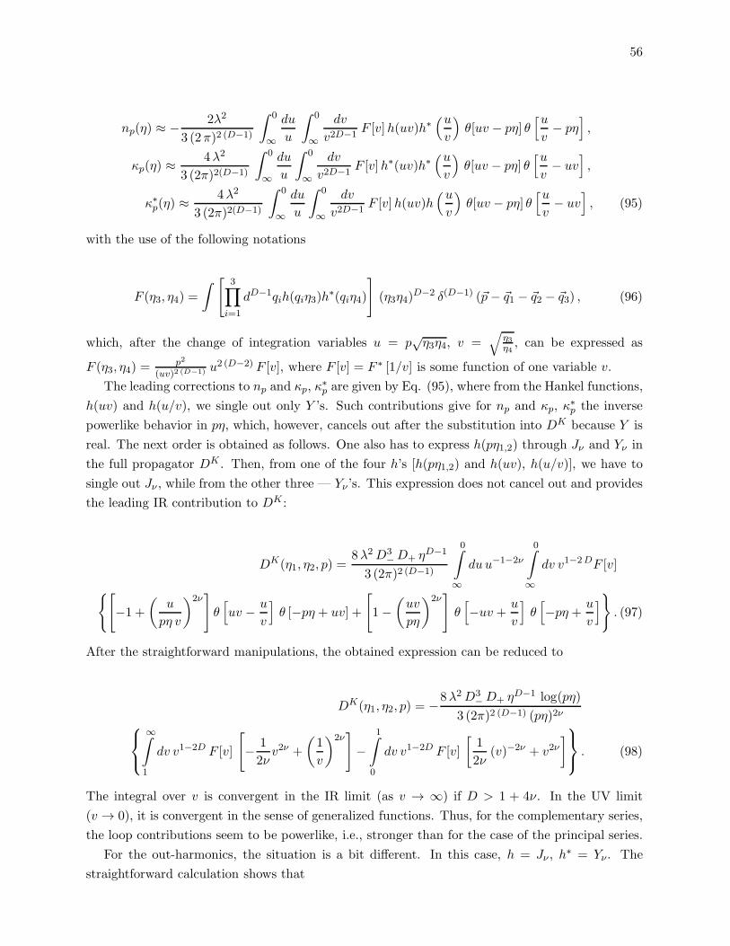
56
np(η) ≈ − 2λ2
3 (2π)2 (D−1)
∫ 0
∞
du
u
∫ 0
∞
dv
v2D−1F [v]h(uv)h∗
(u
v
)
θ[uv − pη] θ[u
v− pη
]
,
κp(η) ≈4λ2
3 (2π)2(D−1)
∫ 0
∞
du
u
∫ 0
∞
dv
v2D−1F [v]h∗(uv)h∗
(u
v
)
θ[uv − pη] θ[u
v− uv
]
,
κ∗p(η) ≈4λ2
3 (2π)2(D−1)
∫ 0
∞
du
u
∫ 0
∞
dv
v2D−1F [v]h(uv)h
(u
v
)
θ[uv − pη] θ[u
v− uv
]
, (95)
with the use of the following notations
F (η3, η4) =
∫
[
3∏
i=1
dD−1qih(qiη3)h∗(qiη4)
]
(η3η4)D−2 δ(D−1) (~p− ~q1 − ~q2 − ~q3) , (96)
which, after the change of integration variables u = p√η3η4, v =
√
η3η4, can be expressed as
F (η3, η4) =p2
(uv)2 (D−1) u2 (D−2) F [v], where F [v] = F ∗ [1/v] is some function of one variable v.
The leading corrections to np and κp, κ∗p are given by Eq. (95), where from the Hankel functions,
h(uv) and h(u/v), we single out only Y ’s. Such contributions give for np and κp, κ∗p the inverse
powerlike behavior in pη, which, however, cancels out after the substitution into DK because Y is
real. The next order is obtained as follows. One also has to express h(pη1,2) through Jν and Yν in
the full propagator DK . Then, from one of the four h’s [h(pη1,2) and h(uv), h(u/v)], we have to
single out Jν , while from the other three — Yν ’s. This expression does not cancel out and provides
the leading IR contribution to DK :
DK(η1, η2, p) =8λ2D3
−D+ ηD−1
3 (2π)2 (D−1)
0∫
∞
duu−1−2ν
0∫
∞
dv v1−2DF [v]
[
−1 +
(
u
pη v
)2ν]
θ[
uv − u
v
]
θ [−pη + uv] +
[
1−(
uv
pη
)2ν]
θ[
−uv + u
v
]
θ[
−pη + u
v
]
. (97)
After the straightforward manipulations, the obtained expression can be reduced to
DK(η1, η2, p) = −8λ2D3−D+ η
D−1 log(pη)
3 (2π)2 (D−1) (pη)2ν
∞∫
1
dv v1−2D F [v]
[
− 1
2νv2ν +
(
1
v
)2ν]
−1∫
0
dv v1−2D F [v]
[
1
2ν(v)−2ν + v2ν
]
. (98)
The integral over v is convergent in the IR limit (as v → ∞) if D > 1 + 4ν. In the UV limit
(v → 0), it is convergent in the sense of generalized functions. Thus, for the complementary series,
the loop contributions seem to be powerlike, i.e., stronger than for the case of the principal series.
For the out-harmonics, the situation is a bit different. In this case, h = Jν , h∗ = Yν. The
straightforward calculation shows that

57
np(η) ∝ λ2D−D+ log(pη)
∫ 1
0dv F [v]v2ν+1−2D ,
κp(η) ∝ λ2D2− (pη)−2ν
∫ 0
1dv F [v] v2ν+1−2D ,
κ∗p(η) ∝ λ2D2+ (pη)2 ν
∫ 1
0dv F [v] v−2ν+1−2D . (99)
After the substitution into the Keldysh propagator, the leading contribution comes from np and
is logarithmic. However, because of the character of these IR contributions for the light fields, we
do not yet understand their physical meaning and think that the kinetic equations obtained above
are not applicable for the fields from the complementary series. In the case of the complementary
series, we do not yet know how to perform the summation of the leading IR contributions from all
loops. But on general physical grounds and from the two-loop result, we expect that light fields
from the complementary series will show stronger IR effects than the heavy ones from the principal
series.
VII. ACKNOWLEDGEMENTS
This work is dedicated to the memory of M.I.Polykarpov.
These notes are based on the lectures given at Scuola Normale Superiore, Pisa, Italy and Max-
Plank-Institute for the Gravitational Physics (Albert-Einstein-Institute), Golm, Germany. I would
like to thank D.Francia, A.Sagnotty, H.Nicolai, S.Theisen and S.Fredenhagen for the hospitality
during my stay in these institutes.
I would like to thank P.Burda, A.Sadofyev, V.Slepukhin and F.Popov for the collaboration on
this project. I would like to acknowledge valuable discussions with A.Roura, D.Marolf, I.Morrison,
A.Morozov, A.Mironov, V.Losyakov, S.Apenko, D.Francia, S.Theisen and A.Polyakov. This work
was partially supported by the Ministry of Education and Science of Russian Federation under the
contract 8207, by the grant ”Leading Scientific Schools” No. NSh-6260.2010.2 and by the grant
RFBR-11-02-01227-a.
[1] E. Schrodinger, Cambridge, UK: Univ. Pr. (2010) 93 p
[2] B. Allen, “Vacuum States In De Sitter Space,” Phys. Rev. D 32, 3136 (1985).
[3] B. Allen and A. Folacci, Phys. Rev. D 35, 3771 (1987).
[4] S. P. Miao, P. J. Mora, N. C. Tsamis and R. P. Woodard, “The Perils of Analytic Continuation,”
arXiv:1306.5410 [gr-qc].
[5] N. C. Tsamis and R. P. Woodard, Class. Quant. Grav. 11, 2969 (1994).
[6] N. C. Tsamis and R. P. Woodard, Phys. Lett. B 292, 269 (1992).
[7] N. C. Tsamis and R. P. Woodard, Commun. Math. Phys. 162, 217 (1994).
[8] N. C. Tsamis and R. P. Woodard, Annals Phys. 238, 1 (1995).
[9] N. C. Tsamis and R. P. Woodard, Nucl. Phys. B 474, 235 (1996) [arXiv:hep-ph/9602315].

58
[10] N. C. Tsamis and R. P. Woodard, Phys. Rev. D 54, 2621 (1996) [arXiv:hep-ph/9602317].
[11] N. C. Tsamis and R. P. Woodard, Annals Phys. 253, 1 (1997) [arXiv:hep-ph/9602316].
[12] J. Garriga and T. Tanaka, Phys. Rev. D 77, 024021 (2008) [arXiv:hep-th/0706.0295].
[13] A. Higuchi, D. Marolf and I. A. Morrison, Class. Quant. Grav. 28, 245012 (2011) [arXiv:1107.2712
[hep-th]].
[14] I. A. Morrison, “On cosmic hair and ”de Sitter breaking” in linearized quantum gravity,”
arXiv:1302.1860 [gr-qc].
[15] G. Perez-Nadal, A. Roura and E. Verdaguer, Class. Quant. Grav. 25, 154013 (2008) [arXiv:gr-
qc/0806.2634].
[16] G. Perez-Nadal, A. Roura and E. Verdaguer, Phys. Rev. D 77, 124033 (2008) [arXiv:0712.2282 [gr-qc]].
[17] G. Perez-Nadal, A. Roura and E. Verdaguer, JCAP 1005, 036 (2010) [arXiv:0911.4870 [gr-qc]].
[18] A. Roura and E. Verdaguer, Int. J. Theor. Phys. 38, 3123 (1999) [arXiv:gr-qc/9904039].
[19] E. Mottola, Phys. Rev. D 31, 754 (1985).
[20] D. Marolf, I. A. Morrison and M. Srednicki, “Perturbative S-matrix for massive scalar fields in global
de Sitter space,” arXiv:1209.6039 [hep-th].
[21] D. Marolf and I. A. Morrison, Phys. Rev. D 82, 105032 (2010) [arXiv:1006.0035 [gr-qc]].
[22] D. Marolf and I. A. Morrison, Gen. Rel. Grav. 43, 3497 (2011) [arXiv:1104.4343 [gr-qc]].
[23] A. Higuchi, D. Marolf, I. A. Morrison, Phys. Rev. D83, 084029 (2011). [arXiv:1012.3415 [gr-qc]].
[24] D. Marolf and I. A. Morrison, Phys. Rev. D 84, 044040 (2011) [arXiv:1010.5327 [gr-qc]].
[25] S. Hollands, Commun. Math. Phys. 319, 1 (2013) [arXiv:1010.5367 [gr-qc]].
[26] S. Hollands, Annales Henri Poincare 13, 1039 (2012) [arXiv:1105.1996 [gr-qc]].
[27] I. Antoniadis, P. O. Mazur and E. Mottola, New J. Phys. 9, 11 (2007) [arXiv:gr-qc/0612068].
[28] E. Mottola, Phys. Rev. D 33, 1616 (1986).
[29] E. Mottola, Phys. Rev. D 33, 2136 (1986).
[30] P. Mazur and E. Mottola, Nucl. Phys. B 278, 694 (1986).
[31] P. R. Anderson, C. Molina-Paris, E. Mottola, Phys. Rev. D80, 084005 (2009). [arXiv:0907.0823 [gr-qc]].
[32] E. Mottola, [arXiv:1008.5006 [gr-qc]].
[33] A. D. Dolgov, M. B. Einhorn and V. I. Zakharov, Phys. Rev. D 52, 717 (1995) [arXiv:gr-qc/9403056].
[34] Acta Phys. Polon. B 26, 65 (1995) [arXiv:gr-qc/9405026].
[35] A. M. Polyakov, Nucl. Phys. B 797, 199 (2008) [arXiv:0709.2899 [hep-th]].
[36] A. M. Polyakov, Nucl. Phys. B 834, 316 (2010) [arXiv:0912.5503 [hep-th]].
[37] A. Higuchi, Class. Quant. Grav. 26, 072001 (2009) [arXiv:0809.1255 [gr-qc]].
[38] A. Higuchi and Y. C. Lee, Class. Quant. Grav. 26, 135019 (2009) [arXiv:0903.3881 [gr-qc]].
[39] E. Alvarez and R. Vidal, JHEP 0910, 045 (2009) [arXiv:0907.2375 [hep-th]].
[40] E. Alvarez and R. Vidal, JCAP 1011, 043 (2010) [arXiv:1004.4867 [hep-th]].
[41] C. P. Burgess, R. Holman, L. Leblond and S. Shandera, JCAP 1010, 017 (2010) [arXiv:1005.3551
[hep-th]].
[42] C. P. Burgess, L. Leblond, R. Holman and S. Shandera, JCAP 1003, 033 (2010) [arXiv:0912.1608
[hep-th]].
[43] S. B. Giddings, M. S. Sloth, JCAP 1007, 015 (2010). [arXiv:1005.3287 [hep-th]].
[44] S. B. Giddings, M. S. Sloth, JCAP 1101, 023 (2011). [arXiv:1005.1056 [hep-th]].
[45] A. Riotto, M. S. Sloth, JCAP 0804, 030 (2008). [arXiv:0801.1845 [hep-ph]].
[46] V. K. Onemli, R. P. Woodard, Class. Quant. Grav. 19, 4607 (2002). [gr-qc/0204065].
[47] V. K. Onemli, R. P. Woodard, Phys. Rev. D70, 107301 (2004). [gr-qc/0406098].
[48] E. O. Kahya, V. K. Onemli, Phys. Rev. D76, 043512 (2007). [gr-qc/0612026].
[49] E. O. Kahya, V. K. Onemli, R. P. Woodard, Phys. Rev. D81, 023508 (2010). [arXiv:0904.4811 [gr-qc]].
59
[50] D. L. Lp. Nacir, F. D. Mazzitelli and L. G. Trombetta, “The Hartree approximation in curved spacetimes
revisited I: the effective potential in de Sitter,” arXiv:1309.0864 [hep-th].
[51] W. Xue, K. Dasgupta, R. Brandenberger, Phys. Rev. D83, 083520 (2011). [arXiv:1103.0285 [hep-th]].
[52] A. M. Polyakov, “Infrared instability of the de Sitter space,” arXiv:1209.4135 [hep-th].
[53] T. S. Bunch and P. C. W. Davies, Proc. Roy. Soc. Lond. A 360, 117 (1978).
[54] N. A. Chernikov and E. A. Tagirov, Ann. Inst. Henri Poincare A 9, 109 (1968).
[55] E. T. Akhmedov, A. V. Sadofyev, Phys. Lett. B 712, 138 (2012) [arXiv:1201.3471 [hep-th]].
[56] D. Krotov, A. M. Polyakov, Nucl. Phys. B849, 410-432 (2011). [arXiv:1012.2107 [hep-th]].
[57] E. T. Akhmedov, JHEP 1201, 066 (2012) [arXiv:1110.2257 [hep-th]].
[58] E. T. Akhmedov, F. K. Popov and V. M. Slepukhin, Phys. Rev. D 88, 024021 (2013) [arXiv:1303.1068
[hep-th]].
[59] L. D. Landau and E. M. Lifshitz, Vol. 10 (Pergamon Press, Oxford, 1975).
[60] A.Kamenev, “Many-body theory of non-equilibrium systems”, arXiv:cond-mat/0412296; Bibliographic
Code: 2004cond.mat.12296K.
[61] E. T. Akhmedov and P. .Burda, Phys. Rev. D 86, 044031 (2012) [arXiv:1202.1202 [hep-th]].
[62] E. T. Akhmedov, Phys. Rev. D 87, 044049 (2013) [arXiv:1209.4448 [hep-th]].
[63] Misner C. W., Wheeler J. A. Gravitation: Charles W. Misner, Kip S. Thorne, John Archibald Wheeler.
“Gravitation”, Macmillan, San Francisco 1973, 1279p; ISBN-9780716703440
[64] W. G. Unruh, Phys. Rev. D 14, 870 (1976).
[65] E. T. Akhmedov and D. Singleton, Int. J. Mod. Phys. A 22, 4797 (2007) [hep-ph/0610391].
[66] E. T. Akhmedov and D. Singleton, Pisma Zh. Eksp. Teor. Fiz. 86, 702 (2007) [arXiv:0705.2525 [hep-th]].
[67] R. Bousso, A. Maloney and A. Strominger, Phys. Rev. D 65, 104039 (2002) [arXiv:hep-th/0112218].
[68] Grib A. A., Mamaev S. G., Mostepanenko V. M. “Quantum effects in strong external fields”, Atomizdat,
Moscow 1980, 296.
Grib A. A., Mamayev S. G., Mostepanenko V. M. Vacuum quantum effects in strong fields. St.
Petersburg : Friedmann Laboratory, 1994.
[69] M. van der Meulen, J. Smit, JCAP 0711, 023 (2007). [arXiv:0707.0842 [hep-th]].
[70] Gradshteyn I. S., Ryzhik I. M., “Table of integrals”, Series, and Products (Academic, New York, 1980),
1.421.
[71] D. P. Jatkar, L. Leblond and A. Rajaraman, Phys. Rev. D 85, 024047 (2012) [arXiv:1107.3513 [hep-th]].
[72] N. Myrhvold, Phys. Rev. D 28 2439 (1983).
[73] D. Boyanovsky, H. J. de Vega and N. G. Sanchez, Phys. Rev. D 71, 023509 (2005)
[arXiv:astro-ph/0409406].
[74] D. Boyanovsky and H. J. de Vega, Phys. Rev. D 70, 063508 (2004) [arXiv:astro-ph/0406287].
[75] D. Boyanovsky, Phys. Rev. D 85, 123525 (2012) [arXiv:1203.3903 [hep-ph]].
[76] D. Boyanovsky, Phys. Rev. D 86, 023509 (2012) [arXiv:1205.3761 [astro-ph.CO]].
[77] J. Bros, H. Epstein, M. Gaudin, U. Moschella and V. Pasquier, “Triangular invariants, three-point
functions and particle stability on the de Sitter universe,” Commun. Math. Phys. 295, 261 (2010)
[arXiv:0901.4223 [hep-th]].
[78] J. Bros, H. Epstein and U. Moschella, Annales Henri Poincare 11, 611 (2010) [arXiv:0812.3513 [hep-th]].
[79] J. Bros, H. Epstein and U. Moschella, “Lifetime of a massive particle in a de Sitter universe,” JCAP
0802, 003 (2008) [arXiv:hep-th/0612184].
[80] G. E. Volovik, “On de Sitter radiation via quantum tunneling,” [arXiv:gr-qc/0803.3367].
JETP Lett. 90, 1 (2009) [arXiv:gr-qc/0905.4639].
[81] E. T. Akhmedov, P. V. Buividovich and D. A. Singleton, Phys. Atom. Nucl. 75, 525 (2012)
[arXiv:0905.2742 [gr-qc]].

60
[82] E. T. Akhmedov, A. Roura and A. Sadofyev, Phys. Rev. D 82, 044035 (2010) [arXiv:1006.3274 [gr-qc]].
[83] E. T. Akhmedov and P. V. Buividovich, “Interacting Field Theories in de Sitter Space are Non-Unitary,”
Phys. Rev. D 78, 104005 (2008) [arXiv:0808.4106 [hep-th]].
[84] E. T. Akhmedov and P. Burda, Phys. Lett. B 687, 267 (2010) [arXiv:0912.3435 [hep-th]].
[85] E. T. Akhmedov, Mod. Phys. Lett. A 25, 2815 (2010) [arXiv:0909.3722 [hep-th]].
[86] E. T. Akhmedov and E. T. Musaev, “Comments on QED with background electric fields,” New J.
Phys. 11, 103048 (2009) [arXiv:0901.0424 [hep-ph]].
[87] A. Youssef and D. Kreimer, “Resummation of infrared logarithms in de Sitter space via Dyson-
Schwinger equations: the ladder-rainbow approximation,” arXiv:1301.3205 [gr-qc].
[88] F. Gautier and J. Serreau, “Solving the Schwinger-Dyson equation for a scalar field in de Sitter space,”
arXiv:1305.5705 [hep-th].