THE OPEN BOOK SERIES 1

ANTS XProceedings of the TenthAlgorithmic Number Theory Symposium

msp

Iterated Coleman integrationfor hyperelliptic curves

Jennifer S. Balakrishnan

THE OPEN BOOK SERIES 1 (2013)

Tenth Algorithmic Number Theory Symposiumdx.doi.org/10.2140/obs.2013.1.41

msp

Iterated Coleman integrationfor hyperelliptic curves

Jennifer S. Balakrishnan

The Coleman integral is a p-adic line integral. Double Coleman integrals onelliptic curves appear in Kim’s nonabelian Chabauty method, the first numericalexamples of which were given by the author, Kedlaya, and Kim. This paperdescribes the algorithms used to produce those examples, as well as techniquesto compute higher iterated integrals on hyperelliptic curves, building on previousjoint work with Bradshaw and Kedlaya.

1. Introduction

In a series of papers in the 1980s, Coleman gave a p-adic theory of integration onthe projective line [8], then on curves and abelian varieties [9; 7]. This integrationtheory relies on locally defined antiderivatives that are extended analytically by theprinciple of Frobenius equivariance. In joint work with Bradshaw and Kedlaya [1],we made this construction explicit and gave algorithms to compute single Colemanintegrals for hyperelliptic curves.

Having algorithms to compute Coleman integrals allows one to compute p-adicregulators in K-theory [8; 7], carry out the method of Chabauty-Coleman forfinding rational points on higher genus curves [15], and utilize Kim’s nonabeliananalogue of the Chabauty method [14].

Kim’s method, in the case of rank-1 elliptic curves, allows one to find integralpoints via the computation of double Coleman integrals. Indeed, Coleman’s theoryof integration is not limited to single integrals; it gives rise to an entire class of

MSC2010: primary 11S80; secondary 11Y35, 11Y50.Keywords: Coleman integration, p-adic integration, iterated Coleman integration, hyperelliptic

curves, nonabelian Chabauty, integral points.

41

42 JENNIFER S. BALAKRISHNAN

locally analytic functions, the Coleman functions, on which antidifferentiation iswell-defined. In other words, one can define iterated p-adic integrals [4; 8]Z Q

P

�n � � � �1

which behave formally like iterated path integralsZ 1

0

Z t1

0

� � �

Z tn�1

0

fn.tn/ � � � f1.t1/ dtn � � � dt1:

Let us fix some notation. Let C be a genus-g hyperelliptic curve over an unram-ified extension K of Qp having good reduction. Let k D Fq denote its residue field,where q D pm. We will assume that C is given by a model of the form y2 D f .x/,where f is a monic separable polynomial with degf D 2gC 1.

Our methods for computing iterated integrals are similar in spirit to those de-tailed in [1]. We begin with algorithms for tiny iterated integrals, use Frobeniusequivariance to write down a linear system yielding the values of integrals betweenpoints in different residue disks, and, if needed, use basic properties of integrationto correct endpoints. We begin with some basic properties of iterated path integrals.

2. Iterated path integrals

We follow the convention of Kim [14] and define our integrals as follows:Z Q

P

�1�2 � � ��n�1�n WD

Z Q

P

�1.R1/

Z R1

P

�2.R2/ � � �

Z Rn�2

P

�n�1.Rn�1/

Z Rn�1

P

�n;

for a collection of dummy parameters R1; : : : ; Rn�1 and 1-forms �1; : : : ; �n.We begin by recalling some key formal properties satisfied by iterated path in-

tegrals [6].

Proposition 2.1. Let �1; : : : ; �n be 1-forms, holomorphic at points P;Q on C .Then:

(1)R PP �1�2 � � � �n D 0,

(2)P

all permutations �RQP !�.i1/!�.i2/ � � �!�.in/ D

QnjD1

RQP !ij ,

(3)RQP !i1 � � �!in D .�1/

nR PQ !in � � �!i1 .

As an easy corollary of Proposition 2.1(2), we have:

Corollary 2.2. For a 1-form !i and points P;Q as before,Z Q

P

!i !i � � �!i D1

nŠ

�Z Q

P

!i

�n:

ITERATED COLEMAN INTEGRATION FOR HYPERELLIPTIC CURVES 43

When possible, we will use this to write an iterated integral in terms of a singleintegral.

3. p-adic cohomology

We briefly recall some p-adic cohomology from [12], necessary for formulatingthe integration algorithms.

Let C 0 be the affine curve obtained by deleting the Weierstrass points from C ,and let ADKŒx; y; z�=.y2� f .x/; yz � 1/ be the coordinate ring of C 0. Let A�

denote the Monsky-Washnitzer weak completion of A; it is the ring consisting ofinfinite sums of the form

1XiD�1

Bi .x/

yi; Bi .x/ 2KŒx�; degBi � 2g;

further subject to the condition that vp.Bi .x// grows faster than a linear functionof i as i !˙1. We make a ring out of these using the relation y2 D f .x/.

These functions are holomorphic on the space over which we integrate, so weconsider odd 1-forms written as

! D g.x; y/dx

2y; g.x; y/ 2 A�:

Any such differential can be written as

! D dF C c0!0C � � �C c2g�1!2g�1; (1)

with F 2 A�; ci 2K, and

!i D xi dx

2y.i D 0; : : : ; 2g� 1/:

Namely, the set of differentials f!ig2g�1iD0 forms a basis of the odd part of the

de Rham cohomology of A�, which we denote as H 1dR.C 0/�.

One computes the p-power Frobenius action �� on H 1dR.C 0/� as follows:

� Let �K denote the unique automorphism lifting Frobenius from Fq to K. Ex-tend �K to A� by setting

�.x/D xp;

�.y/D yp�1C

�.f /.xp/�f .x/p

f .x/p

�12

D yp1XiD0

�12

i

�.�.f /.xp/�f .x/p/i

y2pi:

44 JENNIFER S. BALAKRISHNAN

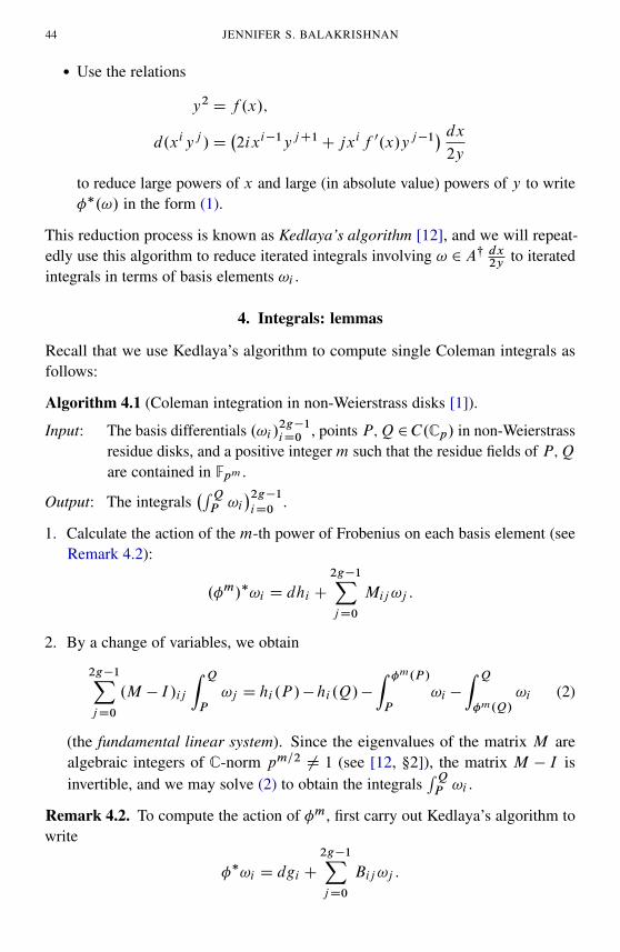
� Use the relations

y2 D f .x/;

d.xiyj /D�2ixi�1yjC1C jxif 0.x/yj�1

� dx2y

to reduce large powers of x and large (in absolute value) powers of y to write��.!/ in the form (1).

This reduction process is known as Kedlaya’s algorithm [12], and we will repeat-edly use this algorithm to reduce iterated integrals involving ! 2 A� dx

2yto iterated

integrals in terms of basis elements !i .

4. Integrals: lemmas

Recall that we use Kedlaya’s algorithm to compute single Coleman integrals asfollows:

Algorithm 4.1 (Coleman integration in non-Weierstrass disks [1]).

Input: The basis differentials .!i /2g�1iD0 , points P;Q 2C.Cp/ in non-Weierstrass

residue disks, and a positive integer m such that the residue fields of P;Qare contained in Fpm .

Output: The integrals�RQP !i

�2g�1iD0

.

1. Calculate the action of the m-th power of Frobenius on each basis element (seeRemark 4.2):

.�m/�!i D dhi C

2g�1XjD0

Mij!j :

2. By a change of variables, we obtain

2g�1XjD0

.M � I /ij

Z Q

P

!j D hi .P /� hi .Q/�

Z �m.P /

P

!i �

Z Q

�m.Q/

!i (2)

(the fundamental linear system). Since the eigenvalues of the matrix M arealgebraic integers of C-norm pm=2 ¤ 1 (see [12, §2]), the matrix M � I isinvertible, and we may solve (2) to obtain the integrals

RQP !i .

Remark 4.2. To compute the action of �m, first carry out Kedlaya’s algorithm towrite

��!i D dgi C

2g�1XjD0

Bij!j :

ITERATED COLEMAN INTEGRATION FOR HYPERELLIPTIC CURVES 45

If we view h; g as column vectors and M;B as matrices, induction on m showsthat

hD �m�1.g/CB�m�2.g/C � � �CB�K.B/ � � ��m�2K .B/g;

M D B�K.B/ � � ��m�1K .B/:

Note, however, that when points P;Q 2 C.Cp/ are in the same residue disk, the“tiny” Coleman integral between them can be computed using a local parametriza-tion, just as in the case of a real-valued line integral. This is also true when theintegrals are iterated (see Section 5).

However, to compute general iterated integrals, we will need to employ theanalogue of “additivity in endpoints” to link integrals between different residuedisks. First, let us consider the case where we are breaking up the path by onepoint.

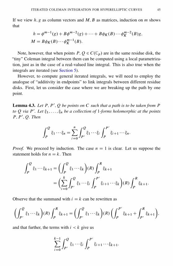
Lemma 4.3. Let P;P 0;Q be points on C such that a path is to be taken from P

to Q via P 0. Let �1; : : : ; �n be a collection of 1-forms holomorphic at the pointsP;P 0;Q. Then

Z Q

P

�1 � � � �n D

nXiD0

Z Q

P 0�1 � � � �i

Z P 0

P

�iC1 � � � �n:

Proof. We proceed by induction. The case n D 1 is clear. Let us suppose thestatement holds for nD k. ThenZ Q

P

�1 � � � �kC1 D

�Z Q

P

�1 � � � �k

�.R/

Z R

P

�kC1

D

� kXiD0

Z Q

P 0�1 � � � �i

Z P 0

P

�iC1 � � � �k

�.R/

Z R

P

�kC1:

Observe that the summand with i D k can be rewritten as�Z Q

P 0�1 � � � �k

�.R/

Z R

P

�kC1 D

�Z Q

P 0�1 � � � �k

�.R/

�Z P 0

P

�kC1C

Z R

P 0�kC1

�;

and that further, the terms with i < k give us

k�1XiD0

Z Q

P 0�1 � � � �i

Z P 0

P

�iC1 � � � �kC1:

46 JENNIFER S. BALAKRISHNAN

Thus we haveZ Q

P

�1 � � � �kC1 D

k�1XiD0

Z Q

P 0�1 � � � �i

Z P 0

P

�iC1 � � � �kC1

C

�Z Q

P 0�1 � � � �k

��Z P 0

P

�kC1

�C

Z Q

P 0�1 � � � �kC1

D

kC1XiD0

Z Q

P 0�1 � � � �i

Z P 0

P

�iC1 � � � �kC1;

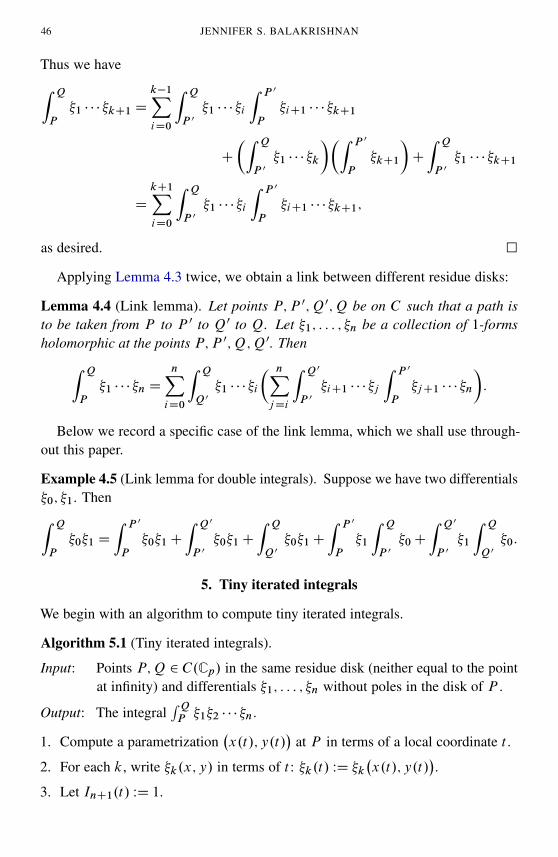
as desired. �

Applying Lemma 4.3 twice, we obtain a link between different residue disks:

Lemma 4.4 (Link lemma). Let points P;P 0;Q0;Q be on C such that a path isto be taken from P to P 0 to Q0 to Q. Let �1; : : : ; �n be a collection of 1-formsholomorphic at the points P;P 0;Q;Q0. ThenZ Q

P

�1 � � � �n D

nXiD0

Z Q

Q0�1 � � � �i

� nXjDi

Z Q0

P 0�iC1 � � � �j

Z P 0

P

�jC1 � � � �n

�:

Below we record a specific case of the link lemma, which we shall use through-out this paper.

Example 4.5 (Link lemma for double integrals). Suppose we have two differentials�0; �1. ThenZ Q

P

�0�1 D

Z P 0

P

�0�1C

Z Q0

P 0�0�1C

Z Q

Q0�0�1C

Z P 0

P

�1

Z Q

P 0�0C

Z Q0

P 0�1

Z Q

Q0�0:

5. Tiny iterated integrals

We begin with an algorithm to compute tiny iterated integrals.

Algorithm 5.1 (Tiny iterated integrals).

Input: Points P;Q 2 C.Cp/ in the same residue disk (neither equal to the pointat infinity) and differentials �1; : : : ; �n without poles in the disk of P .

Output: The integralRQP �1�2 � � � �n.

1. Compute a parametrization�x.t/; y.t/

�at P in terms of a local coordinate t .

2. For each k, write �k.x; y/ in terms of t : �k.t/ WD �k�x.t/; y.t/

�.

3. Let InC1.t/ WD 1.

ITERATED COLEMAN INTEGRATION FOR HYPERELLIPTIC CURVES 47

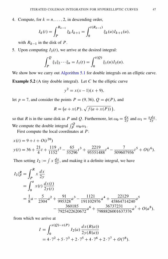
4. Compute, for k D n; : : : ; 2, in descending order,

Ik.t/D

Z Rk�1

P

�kIkC1 D

Z t.Rk�1/

0

�k.u/IkC1.u/;

with Rk�1 in the disk of P .

5. Upon computing I2.t/, we arrive at the desired integral:Z Q

P

�1�2 � � � �n D I1.t/D

Z t.Q/

0

�1.u/I2.u/:

We show how we carry out Algorithm 5.1 for double integrals on an elliptic curve.

Example 5.2 (A tiny double integral). Let C be the elliptic curve

y2 D x.x� 1/.xC 9/;

let p D 7, and consider the points P D .9; 36/;QD �.P /, and

RD�aC x.P /;

pf .aC x.P //

�;

so that R is in the same disk as P and Q. Furthermore, let !0D dx2y

and !1D x dx2y

.

We compute the double integralRQP !0!1.

First compute the local coordinates at P :

x.t/D 9C t CO.t20/

y.t/D 36C21

4t C

119

1152t2�

65

55296t3C

2219

95551488t4�

7

509607936t5CO.t6/:

Then setting I2 WDRx dx2y

, and making it a definite integral, we have

I2jRP D

Z R

P

xdx

2y

D

Z a

0

x.t/dx.t/

2y.t/

D1

8a�

5

2304a2C

91

995328a3�

1121

191102976a4C

22129

45864714240a5

�360185

7925422620672a6C

36737231

7988826001637376a7CO.a8/;

from which we arrive at

I D

Z x.Q/�x.P /

0

I2.a/dx.R.a//

2y.R.a//

D 4 � 72C 5 � 73C 2 � 75C 4 � 76C 2 � 77CO.78/:

48 JENNIFER S. BALAKRISHNAN

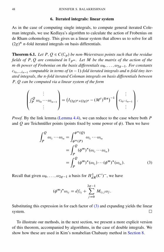
6. Iterated integrals: linear system

As in the case of computing single integrals, to compute general iterated Cole-man integrals, we use Kedlaya’s algorithm to calculate the action of Frobenius onde Rham cohomology. This gives us a linear system that allows us to solve for all.2g/n n-fold iterated integrals on basis differentials.

Theorem 6.1. Let P;Q 2 C.Cp/ be non-Weierstrass points such that the residuefields of P;Q are contained in Fpm . Let M be the matrix of the action of them-th power of Frobenius on the basis differentials !0; : : : ; !2g�1. For constantsci0;:::;in�1

computable in terms of .n� 1/-fold iterated integrals and n-fold tiny iter-ated integrals, the n-fold iterated Coleman integrals on basis differentials betweenP;Q can be computed via a linear system of the form0BB@

:::RQP !i0 � � �!in�1

:::

1CCAD �I.2g/n�.2g/n � .M t /˝n��1

0BB@:::

ci0���in�1

:::

1CCA :Proof. By the link lemma (Lemma 4.4), we can reduce to the case where both Pand Q are Teichmüller points (points fixed by some power of �). Then we haveZ Q

P

!ii � � �!in D

Z �m.Q/

�m.P /

!ii � � �!in

D

Z Q

P

.�m/�.!ii � � �!in/

D

Z Q

P

.�m/�.!ii / � � � .�m/�.!in/: (3)

Recall that given !0; : : : ; !2g�1 a basis for H 1dR.C 0/�, we have

.�m/�!i` D dfi` C

2g�1XjD0

Mi`j!j :

Substituting this expression in for each factor of (3) and expanding yields the linearsystem. �

To illustrate our methods, in the next section, we present a more explicit versionof this theorem, accompanied by algorithms, in the case of double integrals. Weshow how these are used in Kim’s nonabelian Chabauty method in Section 8.

ITERATED COLEMAN INTEGRATION FOR HYPERELLIPTIC CURVES 49

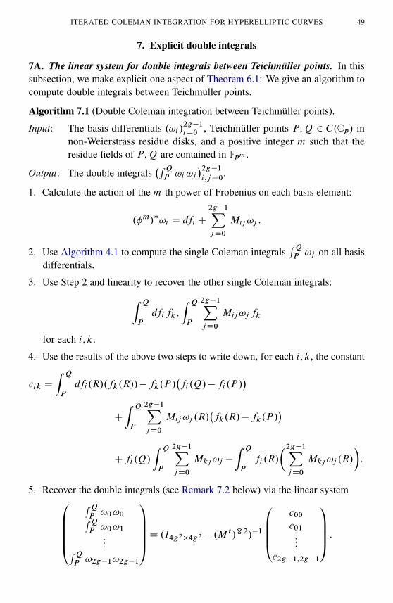
7. Explicit double integrals

7A. The linear system for double integrals between Teichmüller points. In thissubsection, we make explicit one aspect of Theorem 6.1: We give an algorithm tocompute double integrals between Teichmüller points.

Algorithm 7.1 (Double Coleman integration between Teichmüller points).

Input: The basis differentials .!i /2g�1iD0 , Teichmüller points P;Q 2 C.Cp/ in

non-Weierstrass residue disks, and a positive integer m such that theresidue fields of P;Q are contained in Fpm .

Output: The double integrals�RQP !i !j

�2g�1i;jD0

.

1. Calculate the action of the m-th power of Frobenius on each basis element:

.�m/�!i D dfi C

2g�1XjD0

Mij!j :

2. Use Algorithm 4.1 to compute the single Coleman integralsRQP !j on all basis

differentials.

3. Use Step 2 and linearity to recover the other single Coleman integrals:Z Q

P

dfifk;

Z Q

P

2g�1XjD0

Mij!jfk

for each i; k.

4. Use the results of the above two steps to write down, for each i; k, the constant

cik D

Z Q

P

dfi .R/.fk.R//�fk.P /�fi .Q/�fi .P /

�C

Z Q

P

2g�1XjD0

Mij!j .R/�fk.R/�fk.P /

�

Cfi .Q/

Z Q

P

2g�1XjD0

Mkj!j �

Z Q

P

fi .R/

�2g�1XjD0

Mkj!j .R/

�:

5. Recover the double integrals (see Remark 7.2 below) via the linear system0BBBB@RQP !0!0RQP !0!1:::RQ

P !2g�1!2g�1

1CCCCAD .I4g2�4g2 � .M t /˝2/�1

0BBB@c00c01:::

c2g�1;2g�1

1CCCA :

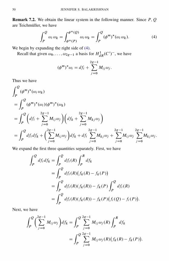
50 JENNIFER S. BALAKRISHNAN

Remark 7.2. We obtain the linear system in the following manner. Since P;Qare Teichmüller, we haveZ Q

P

!i !k D

Z �m.Q/

�m.P /

!i !k D

Z Q

P

.�m/�.!i !k/: (4)

We begin by expanding the right side of (4).Recall that given !0; : : : ; !2g�1 a basis for H 1

dR.C 0/�, we have

.�m/�!i D dfi C

2g�1XjD0

Mij!j :

Thus we haveZ Q

P

.�m/�.!i !k/

D

Z Q

P

.�m/�.!i /.�m/�.!k/

D

Z Q

P

�dfi C

2g�1XjD0

Mij!j

��dfkC

2g�1XjD0

Mkj!j

�

D

Z Q

P

dfidfkC

�2g�1XjD0

Mij!j

�dfkC dfi

2g�1XjD0

Mkj!j C

2g�1XjD0

Mij!j

2g�1XjD0

Mkj!j :

We expand the first three quantities separately. First, we haveZ Q

P

dfidfk D

Z Q

P

dfi .R/

Z R

P

dfk

D

Z Q

P

dfi .R/�fk.R/�fk.P /

�D

Z Q

P

dfi .R/.fk.R//�fk.P /

Z Q

P

dfi .R/

D

Z Q

P

dfi .R/.fk.R//�fk.P /�fi .Q/�fi .P /

�:

Next, we haveZ Q

P

�2g�1XjD0

Mij!j

�dfk D

Z Q

P

2g�1XjD0

Mij!j .R/

Z R

P

dfk

D

Z Q

P

2g�1XjD0

Mij!j .R/�fk.R/�fk.P /

�:

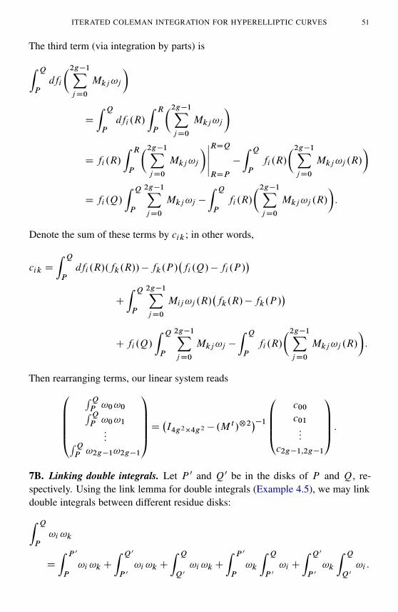
ITERATED COLEMAN INTEGRATION FOR HYPERELLIPTIC CURVES 51

The third term (via integration by parts) is

Z Q

P

dfi

�2g�1XjD0

Mkj!j

�

D

Z Q

P

dfi .R/

Z R

P

�2g�1XjD0

Mkj!j

�

D fi .R/

Z R

P

�2g�1XjD0

Mkj!j

�ˇˇRDQ

RDP

�

Z Q

P

fi .R/

�2g�1XjD0

Mkj!j .R/

�

D fi .Q/

Z Q

P

2g�1XjD0

Mkj!j �

Z Q

P

fi .R/

�2g�1XjD0

Mkj!j .R/

�:

Denote the sum of these terms by cik; in other words,

cik D

Z Q

P

dfi .R/.fk.R//�fk.P /�fi .Q/�fi .P /

�C

Z Q

P

2g�1XjD0

Mij!j .R/�fk.R/�fk.P /

�

Cfi .Q/

Z Q

P

2g�1XjD0

Mkj!j �

Z Q

P

fi .R/

�2g�1XjD0

Mkj!j .R/

�:

Then rearranging terms, our linear system reads0BBBB@RQP !0!0RQP !0!1:::RQ

P !2g�1!2g�1

1CCCCAD �I4g2�4g2 � .M t /˝2��1

0BBB@c00c01:::

c2g�1;2g�1

1CCCA :

7B. Linking double integrals. Let P 0 and Q0 be in the disks of P and Q, re-spectively. Using the link lemma for double integrals (Example 4.5), we may linkdouble integrals between different residue disks:Z Q

P

!i !k

D

Z P 0

P

!i !kC

Z Q0

P 0!i !kC

Z Q

Q0!i !kC

Z P 0

P

!k

Z Q

P 0!i C

Z Q0

P 0!k

Z Q

Q0!i :

52 JENNIFER S. BALAKRISHNAN

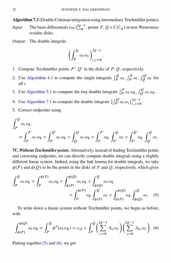
Algorithm 7.3 (Double Coleman integration using intermediary Teichmüller points).

Input: The basis differentials .!i /2g�1iD0 , points P;Q 2C.Cp/ in non-Weierstrass

residue disks.

Output: The double integrals �Z Q

P

!i !j

�2g�1i;jD0

:

1. Compute Teichmüller points P 0;Q0 in the disks of P;Q, respectively.

2. Use Algorithm 4.1 to compute the single integralsRQP !i ;

R PP 0 !i ;

RQ0Q !i for

all i .

3. Use Algorithm 5.1 to compute the tiny double integralsR PP 0 !i !k;

RQQ0 !i !k .

4. Use Algorithm 7.1 to compute the double integrals˚RQ0P 0 !i !j

2g�1i;jD0

.

5. Correct endpoints usingZ Q

P

!i !k

D

Z P 0

P

!i !kC

Z Q0

P 0!i !kC

Z Q

Q0!i !kC

Z P 0

P

!k

Z Q

P 0!i C

Z Q0

P 0!k

Z Q

Q0!i :

7C.Without Teichmüller points.Alternatively, instead of finding Teichmüller pointsand correcting endpoints, we can directly compute double integrals using a slightlydifferent linear system. Indeed, using the link lemma for double integrals, we take�.P / and �.Q/ to be the points in the disks of P and Q, respectively, which givesZ Q

P

!i !k D

Z �.P /

P

!i !kC

Z �.Q/

�.P /

!i !kC

Z Q

�.Q/

!i !k

C

Z �.P /

P

!k

Z Q

�.P/

!i C

Z �.Q/

�.P /

!k

Z Q

�.Q/

!i : (5)

To write down a linear system without Teichmüller points, we begin as before,withZ �.Q/

�.P /

!i !k D

Z Q

P

��.!i !k/D cikC

Z Q

P

�2g�1XjD0

Aij!j

��2g�1XjD0

Akj!j

�: (6)

Putting together (5) and (6), we get

ITERATED COLEMAN INTEGRATION FOR HYPERELLIPTIC CURVES 530BB@:::RQ

P !i !k:::

1CCAD �I4g2�4g2 � .M t /˝2��1

�

0BBBBB@:::

cik �R P�.P/ !i !k �

�RQP !i

��R P�.P/ !k

���R �.Q/Q !i

��R �.Q/�.P /

!k�CRQ�.Q/

!i !k:::

1CCCCCA : (7)

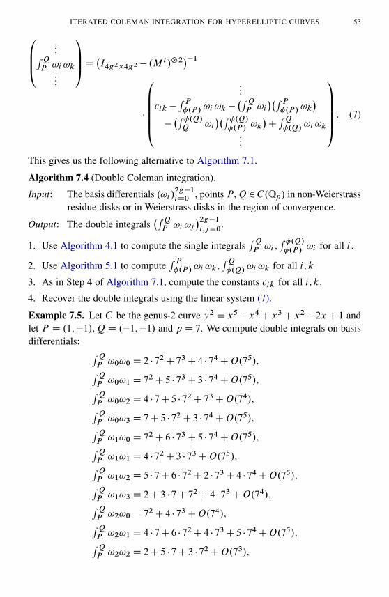
This gives us the following alternative to Algorithm 7.1.

Algorithm 7.4 (Double Coleman integration).

Input: The basis differentials .!i /2g�1iD0 , points P;Q2C.Qp/ in non-Weierstrass

residue disks or in Weierstrass disks in the region of convergence.

Output: The double integrals�RQP !i !j

�2g�1i;jD0

.

1. Use Algorithm 4.1 to compute the single integralsRQP !i ;

R �.Q/�.P /

!i for all i .

2. Use Algorithm 5.1 to computeR P�.P/ !i !k;

RQ�.Q/

!i !k for all i; k

3. As in Step 4 of Algorithm 7.1, compute the constants cik for all i; k.

4. Recover the double integrals using the linear system (7).

Example 7.5. Let C be the genus-2 curve y2 D x5� x4C x3C x2� 2xC 1 andlet P D .1;�1/;QD .�1;�1/ and p D 7. We compute double integrals on basisdifferentials: RQ

P !0!0 D 2 � 72C 73C 4 � 74CO.75/;RQ

P !0!1 D 72C 5 � 73C 3 � 74CO.75/;RQ

P !0!2 D 4 � 7C 5 � 72C 73CO.74/;RQ

P !0!3 D 7C 5 � 72C 3 � 74CO.75/;RQ

P !1!0 D 72C 6 � 73C 5 � 74CO.75/;RQ

P !1!1 D 4 � 72C 3 � 73CO.75/;RQ

P !1!2 D 5 � 7C 6 � 72C 2 � 73C 4 � 74CO.75/;RQ

P !1!3 D 2C 3 � 7C 72C 4 � 73CO.74/;RQ

P !2!0 D 72C 4 � 73CO.74/;RQ

P !2!1 D 4 � 7C 6 � 72C 4 � 73C 5 � 74CO.75/;RQ

P !2!2 D 2C 5 � 7C 3 � 72CO.73/;

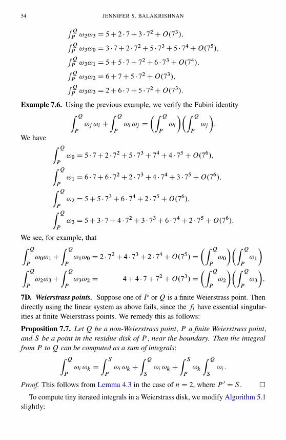
54 JENNIFER S. BALAKRISHNANRQP !2!3 D 5C 2 � 7C 3 � 7

2CO.73/;RQP !3!0 D 3 � 7C 2 � 7

2C 5 � 73C 5 � 74CO.75/;RQP !3!1 D 5C 5 � 7C 7

2C 6 � 73CO.74/;RQP !3!2 D 6C 7C 5 � 7

2CO.73/;RQP !3!3 D 2C 6 � 7C 5 � 7

2CO.73/:

Example 7.6. Using the previous example, we verify the Fubini identityZ Q

P

!j !i C

Z Q

P

!i !j D

�Z Q

P

!i

��Z Q

P

!j

�:

We have Z Q

P

!0 D 5 � 7C 2 � 72C 5 � 73C 74C 4 � 75CO.76/;Z Q

P

!1 D 6 � 7C 6 � 72C 2 � 73C 4 � 74C 3 � 75CO.76/;Z Q

P

!2 D 5C 5 � 73C 6 � 74C 2 � 75CO.76/;Z Q

P

!3 D 5C 3 � 7C 4 � 72C 3 � 73C 6 � 74C 2 � 75CO.76/:

We see, for example, thatZ Q

P

!0!1C

Z Q

P

!1!0 D 2 � 72C 4 � 73C 2 � 74CO.75/D

�Z Q

P

!0

��Z Q

P

!1

�Z Q

P

!2!3C

Z Q

P

!3!2 D 4C 4 � 7C 72CO.73/D

�Z Q

P

!2

��Z Q

P

!3

�:

7D. Weierstrass points. Suppose one of P or Q is a finite Weierstrass point. Thendirectly using the linear system as above fails, since the fi have essential singular-ities at finite Weierstrass points. We remedy this as follows:

Proposition 7.7. Let Q be a non-Weierstrass point, P a finite Weierstrass point,and S be a point in the residue disk of P , near the boundary. Then the integralfrom P to Q can be computed as a sum of integrals:Z Q

P

!i !k D

Z S

P

!i !kC

Z Q

S

!i !kC

Z S

P

!k

Z Q

S

!i :

Proof. This follows from Lemma 4.3 in the case of nD 2, where P 0 D S . �To compute tiny iterated integrals in a Weierstrass disk, we modify Algorithm 5.1

slightly:

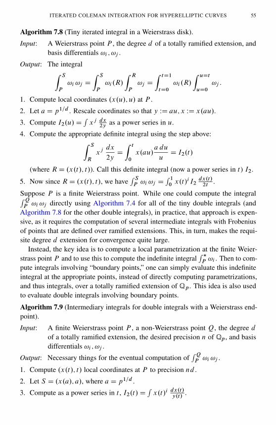
ITERATED COLEMAN INTEGRATION FOR HYPERELLIPTIC CURVES 55

Algorithm 7.8 (Tiny iterated integral in a Weierstrass disk).

Input: A Weierstrass point P , the degree d of a totally ramified extension, andbasis differentials !i ; !j .

Output: The integralZ S

P

!i !j D

Z S

P

!i .R/

Z R

P

!j D

Z tD1

tD0

!i .R/

Z uDt

uD0

!j :

1. Compute local coordinates .x.u/; u/ at P .

2. Let aD p1=d . Rescale coordinates so that y WD au; x WD x.au/.

3. Compute I2.u/DRxj dx

2yas a power series in u.

4. Compute the appropriate definite integral using the step above:Z S

R

xjdx

2yD

Z t

0

x.au/a du

uD I2.t/

(where RD .x.t/; t/). Call this definite integral (now a power series in t ) I2.

5. Now since RD .x.t/; t/, we haveR SP !i !j D

R 10 x.t/

iI2dx.t/2t

.

Suppose P is a finite Weierstrass point. While one could compute the integralRQP !i !j directly using Algorithm 7.4 for all of the tiny double integrals (and

Algorithm 7.8 for the other double integrals), in practice, that approach is expen-sive, as it requires the computation of several intermediate integrals with Frobeniusof points that are defined over ramified extensions. This, in turn, makes the requi-site degree d extension for convergence quite large.

Instead, the key idea is to compute a local parametrization at the finite Weier-strass point P and to use this to compute the indefinite integral

R �P !i . Then to com-

pute integrals involving “boundary points,” one can simply evaluate this indefiniteintegral at the appropriate points, instead of directly computing parametrizations,and thus integrals, over a totally ramified extension of Qp. This idea is also usedto evaluate double integrals involving boundary points.

Algorithm 7.9 (Intermediary integrals for double integrals with a Weierstrass end-point).

Input: A finite Weierstrass point P , a non-Weierstrass point Q, the degree dof a totally ramified extension, the desired precision n of Qp, and basisdifferentials !i ; !j .

Output: Necessary things for the eventual computation ofRQP !i !j .

1. Compute .x.t/; t/ local coordinates at P to precision nd .

2. Let S D .x.a/; a/, where aD p1=d .

3. Compute as a power series in t , I2.t/DRx.t/i dx.t/

y.t/.

56 JENNIFER S. BALAKRISHNAN

4. Compute the definite integralR SP !i D I2.a/.

5. For all i < j , compute the definite integralR SP !i !j via Algorithm 5.1. Keep

the intermediary indefinite integral.

6. For all i D j , use the fact thatR SP !i !j D

12

�R SP !i

�2 to compute the doubleintegral in terms of the single integral.

7. For all i >j , use the fact thatR SP !i !j D�

R SP !j !iC

R SP !i

R SP !j to computeR S

P !i !j (instead of directly computing it as a double integral).

8. ComputeR �.S/S !i D

R �.S/P !i �

R SP !i by the indefinite integral in Step 3. Use

this to deduceR �.S/S !i !j for i D j .

9. Use the indefinite integral in Step 5 to getR �.S/S !i !j for i < j .

10. Repeat the trick in Step 7 to getR �.S/S !i !j for i > j .

11. ComputeR �.Q/Q !i and use it to deduce

R �.Q/Q !i !j for i D j .

12. ComputeR �.Q/Q !i !j for i < j .

13. Repeat the trick in Step 7 to getR �.Q/Q !i !j for i < j .

14. UseRQS !i D

RQP !i �

R SP !i to get

RQS !i .

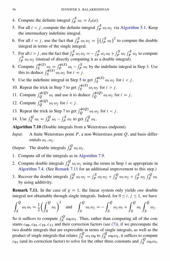
Algorithm 7.10 (Double integrals from a Weierstrass endpoint).

Input: A finite Weierstrass point P , a non-Weierstrass point Q, and basis differ-entials !i ; !j .

Output: The double integralsRQP !i !j .

1. Compute all of the integrals as in Algorithm 7.9.

2. Compute double integralsRQS !i !j using the terms in Step 1 as appropriate in

Algorithm 7.4. (See Remark 7.11 for an additional improvement to this step.)

3. Recover the double integralsRQP !i !j D

R SP !i !j C

RQS !i !j C

R SP !j

RQS !i

by using additivity.

Remark 7.11. In the case of g D 1, the linear system only yields one doubleintegral not obtainable through single integrals. Indeed, for 0� i; j � 1, we haveZ Q

S

!i !i D1

2

�Z Q

S

!i

�2and

Z Q

S

!i !j D�

Z Q

S

!j !i C

Z Q

S

!i

Z Q

S

!j :

So it suffices to computeRQS !0!1. Thus, rather than computing all of the con-

stants c00; c01; c10; c11 and their correction factors (see (7)), if we precompute thetwo double integrals that are expressible in terms of single integrals, as well as theproduct of single integrals that relates

RQS !1!0 to

RQS !0!1, it suffices to compute

c01 (and its correction factor) to solve for the other three constants andRQS !0!1.

ITERATED COLEMAN INTEGRATION FOR HYPERELLIPTIC CURVES 57

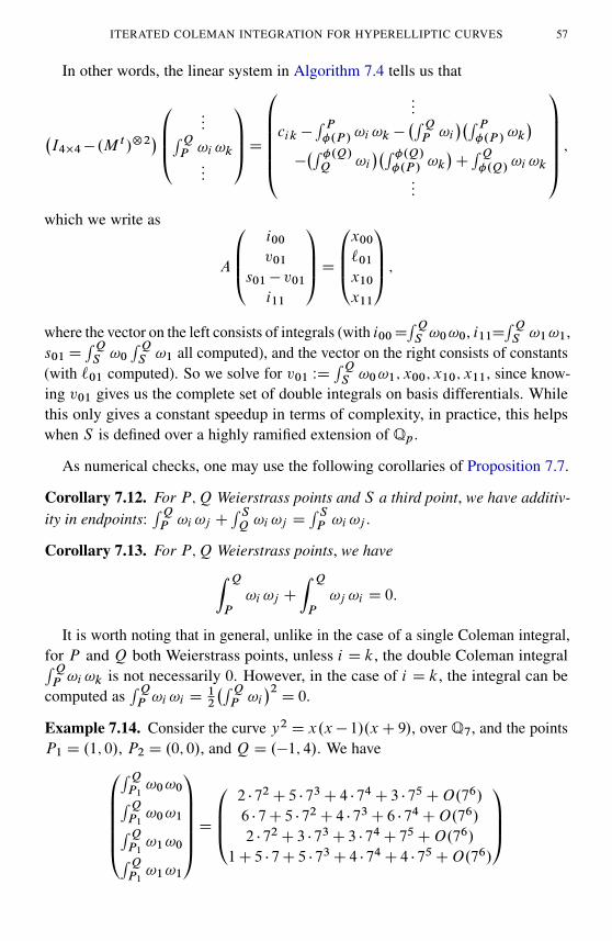
In other words, the linear system in Algorithm 7.4 tells us that

�I4�4� .M

t /˝2�0BB@

:::RQP !i !k:::

1CCAD0BBBBB@

:::

cik �R P�.P/ !i !k �

�RQP !i

��R P�.P/ !k

���R �.Q/Q !i

��R �.Q/�.P /

!k�CRQ�.Q/

!i !k:::

1CCCCCA ;which we write as

A

0BB@i00v01

s01� v01i11

1CCAD0BB@x00`01x10x11

1CCA ;where the vector on the left consists of integrals (with i00D

RQS !0!0, i11D

RQS !1!1,

s01DRQS !0

RQS !1 all computed), and the vector on the right consists of constants

(with `01 computed). So we solve for v01 WDRQS !0!1; x00; x10; x11, since know-

ing v01 gives us the complete set of double integrals on basis differentials. Whilethis only gives a constant speedup in terms of complexity, in practice, this helpswhen S is defined over a highly ramified extension of Qp.

As numerical checks, one may use the following corollaries of Proposition 7.7.

Corollary 7.12. For P;Q Weierstrass points and S a third point, we have additiv-ity in endpoints:

RQP !i !j C

R SQ !i !j D

R SP !i !j .

Corollary 7.13. For P;Q Weierstrass points, we haveZ Q

P

!i !j C

Z Q

P

!j !i D 0:

It is worth noting that in general, unlike in the case of a single Coleman integral,for P and Q both Weierstrass points, unless i D k, the double Coleman integralRQP !i !k is not necessarily 0. However, in the case of i D k, the integral can be

computed asRQP !i !i D

12

�RQP !i

�2D 0.

Example 7.14. Consider the curve y2 D x.x� 1/.xC 9/, over Q7, and the pointsP1 D .1; 0/, P2 D .0; 0/, and QD .�1; 4/. We have0BBBBB@

RQP1!0!0RQ

P1!0!1RQ

P1!1!0RQ

P1!1!1

1CCCCCAD0BB@2 � 72C 5 � 73C 4 � 74C 3 � 75CO.76/

6 � 7C 5 � 72C 4 � 73C 6 � 74CO.76/

2 � 72C 3 � 73C 3 � 74C 75CO.76/

1C 5 � 7C 5 � 73C 4 � 74C 4 � 75CO.76/

1CCA

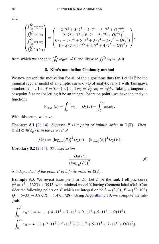
58 JENNIFER S. BALAKRISHNAN

and 0BBBBB@

RQP2!0!0RQ

P2!0!1RQ

P2!1!0RQ

P2!1!1

1CCCCCAD0BB@

2 � 72C 5 � 73C 4 � 74C 3 � 75CO.76/

2 � 72C 73C 6 � 74C 5 � 75CO.76/

6 � 7C 5 � 72C 6 � 73C 3 � 74C 3 � 75CO.76/

1C 5 � 7C 5 � 73C 4 � 74C 4 � 75CO.76/

1CCA ;

from which we see thatR P2

P1!0!1 ¤ 0 and likewise

R P2

P1!1!0 ¤ 0.

8. Kim’s nonabelian Chabauty method

We now present the motivation for all of the algorithms thus far. Let C=Z be theminimal regular model of an elliptic curve C=Q of analytic rank 1 with Tamagawanumbers all 1. Let X D C� f1g and !0 D dx

2y; !1 D

x dx2y

. Taking a tangentialbasepoint b at1 (or letting b be an integral 2-torsion point), we have the analyticfunctions

log!0.z/D

Z z

b

!0; D2.z/D

Z z

b

!0!1:

With this setup, we have:

Theorem 8.1 [2; 14]. Suppose P is a point of infinite order in C.Z/. ThenX.Z/� C.Zp/ is in the zero set of

f .z/ WD�log!0

.P /�2D2.z/�

�log!0

.z/�2D2.P /:

Corollary 8.2 [2; 14]. The expression

D2.P /�log!0

.P /�2 (8)

is independent of the point P of infinite order in C.Z/.

Example 8.3. We revisit Example 1 in [2]. Let E be the rank-1 elliptic curvey2D x3�1323xC3942, with minimal model E having Cremona label 65a1. Con-sider the following points on E which are integral on E: b D .3; 0/, P D .39; 108/,QD .�33;�108/, RD .147; 1728/. Using Algorithm 7.10, we compute the inte-gralsZ P

b

!0!1 D 4 � 11C 4 � 112C 7 � 113C 9 � 114C 5 � 116CO.117/;Z P

b

!0 D 4 � 11C 7 � 112C 9 � 113C 3 � 114C 5 � 115C 7 � 116CO.117/;

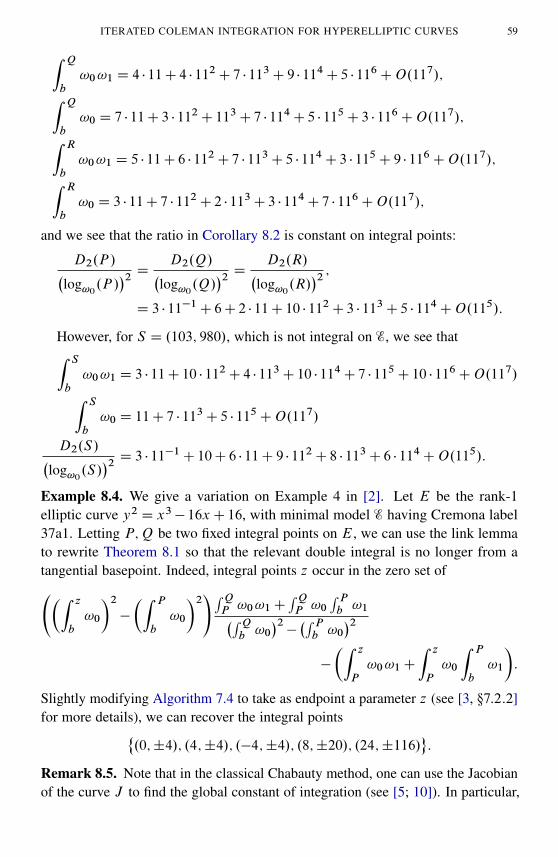
ITERATED COLEMAN INTEGRATION FOR HYPERELLIPTIC CURVES 59Z Q

b

!0!1 D 4 � 11C 4 � 112C 7 � 113C 9 � 114C 5 � 116CO.117/;Z Q

b

!0 D 7 � 11C 3 � 112C 113C 7 � 114C 5 � 115C 3 � 116CO.117/;Z R

b

!0!1 D 5 � 11C 6 � 112C 7 � 113C 5 � 114C 3 � 115C 9 � 116CO.117/;Z R

b

!0 D 3 � 11C 7 � 112C 2 � 113C 3 � 114C 7 � 116CO.117/;

and we see that the ratio in Corollary 8.2 is constant on integral points:

D2.P /�log!0

.P /�2 D D2.Q/�

log!0.Q/

�2 D D2.R/�log!0

.R/�2 ;

D 3 � 11�1C 6C 2 � 11C 10 � 112C 3 � 113C 5 � 114CO.115/:

However, for S D .103; 980/, which is not integral on E, we see thatZ S

b

!0!1 D 3 � 11C 10 � 112C 4 � 113C 10 � 114C 7 � 115C 10 � 116CO.117/Z S

b

!0 D 11C 7 � 113C 5 � 115CO.117/

D2.S/�log!0

.S/�2 D 3 � 11�1C 10C 6 � 11C 9 � 112C 8 � 113C 6 � 114CO.115/:

Example 8.4. We give a variation on Example 4 in [2]. Let E be the rank-1elliptic curve y2 D x3� 16xC 16, with minimal model E having Cremona label37a1. Letting P;Q be two fixed integral points on E, we can use the link lemmato rewrite Theorem 8.1 so that the relevant double integral is no longer from atangential basepoint. Indeed, integral points z occur in the zero set of �Z z

b

!0

�2�

�Z P

b

!0

�2!RQP !0!1C

RQP !0

R Pb !1�RQ

b!0�2��R Pb !0

�2�

�Z z

P

!0!1C

Z z

P

!0

Z P

b

!1

�:

Slightly modifying Algorithm 7.4 to take as endpoint a parameter z (see [3, �7:2:2]for more details), we can recover the integral points˚

.0;˙4/; .4;˙4/; .�4;˙4/; .8;˙20/; .24;˙116/:

Remark 8.5. Note that in the classical Chabauty method, one can use the Jacobianof the curve J to find the global constant of integration (see [5; 10]). In particular,

60 JENNIFER S. BALAKRISHNAN

the points on J form a Z-module and we have multiplication-by-n morphismsŒn�WJ.Qp/! J.Qp/, which gives n

RQP ! D

R Œn�.Q/Œn�.P /

!. By choosing n carefully,we can ensure that Œn�P and Œn�Q both lie in the residue disk of the identity, andpulling back to the curve, all integrals can be computed by tiny integrals. Foriterated integrals, we do not have appropriate endomorphisms available.

Acknowledgments

The author thanks Kiran Kedlaya and Nils Bruin for several helpful conversations,William Stein for access to the computer sage.math.washington.edu, and thereferees for useful suggestions. This work was done as part of the author’s doctoralthesis at MIT, during which she was supported by an NSF Graduate Fellowship andan NDSEG Fellowship. This paper was prepared for submission while the authorwas supported by NSF grant DMS-1103831.

References

[1] Jennifer S. Balakrishnan, Robert W. Bradshaw, and Kiran S. Kedlaya, Explicit Coleman inte-gration for hyperelliptic curves, in Hanrot et al. [11], 2010, pp. 16–31. MR 2012b:14048

[2] Jennifer S. Balakrishnan, Kiran S. Kedlaya, and Minhyong Kim, Appendix and erratum to“Massey products for elliptic curves of rank 1”, J. Amer. Math. Soc. 24 (2011), no. 1, 281–291.MR 2011m:11108

[3] Jennifer Sayaka Balakrishnan, Coleman integration for hyperelliptic curves: algorithms andapplications, Ph.D. thesis, Department of Mathematics, Massachusetts Institute of Technology,2011. http://hdl.handle.net/1721.1/67785

[4] Amnon Besser, Coleman integration using the Tannakian formalism, Math. Ann. 322 (2002),no. 1, 19–48. MR 2003d:11176

[5] Nils Bruin, Chabauty methods using elliptic curves, J. Reine Angew. Math. 562 (2003), 27–49.MR 2004j:11051

[6] Kuo-tsai Chen, Algebras of iterated path integrals and fundamental groups, Trans. Amer. Math.Soc. 156 (1971), 359–379. MR 43 #1069

[7] Robert Coleman and Ehud de Shalit, p-adic regulators on curves and special values of p-adicL-functions, Invent. Math. 93 (1988), no. 2, 239–266. MR 89k:11041

[8] Robert F. Coleman, Dilogarithms, regulators and p-adic L-functions, Invent. Math. 69 (1982),no. 2, 171–208. MR 84a:12021

[9] , Torsion points on curves and p-adic abelian integrals, Ann. of Math. .2/ 121 (1985),no. 1, 111–168. MR 86j:14014

[10] E. V. Flynn, Bjorn Poonen, and Edward F. Schaefer, Cycles of quadratic polynomials and ratio-nal points on a genus-2 curve, Duke Math. J. 90 (1997), no. 3, 435–463. MR 98j:11048

[11] Guillaume Hanrot, François Morain, and Emmanuel Thomé (eds.), Algorithmic number theory:Proceedings of the 9th Biennial International Symposium (ANTS-IX) held in Nancy, July 19–23,2010, Lecture Notes in Computer Science, no. 6197, Berlin, Springer, 2010. MR 2011g:11002

[12] Kiran S. Kedlaya, Counting points on hyperelliptic curves using Monsky-Washnitzer cohomol-ogy, J. Ramanujan Math. Soc. 16 (2001), no. 4, 323–338, errata: [13]. MR 2002m:14019

ITERATED COLEMAN INTEGRATION FOR HYPERELLIPTIC CURVES 61

[13] , Errata for: “Counting points on hyperelliptic curves using Monsky-Washnitzer coho-mology”, J. Ramanujan Math. Soc. 18 (2003), no. 4, 417–418. MR 2005c:14027

[14] Minhyong Kim, Massey products for elliptic curves of rank 1, J. Amer. Math. Soc. 23 (2010),no. 3, 725–747. MR 2012b:11091

[15] William McCallum and Bjorn Poonen, The method of Chabauty and Coleman, preprint, 2010.http://math.mit.edu/~poonen/papers/chabauty.pdf

JENNIFER S. BALAKRISHNAN: jen@math.harvard.eduDepartment of Mathematics, Harvard University, 1 Oxford Street, Cambridge, MA 02138, USA

msp

VOLUME EDITORS

Everett W. HoweCenter for Communications Research

4320 Westerra CourtSan Diego, CA 92121-1969

United States

Kiran S. KedlayaDepartment of Mathematics

University of California, San Diego9500 Gilman Drive #0112La Jolla, CA 92093-0112

Front cover artwork based on a detail ofChicano Legacy 40 Años ©2010 Mario Torero.

The contents of this work are copyrighted by MSP or the respective authors.All rights reserved.

Electronic copies can be obtained free of charge from http://msp.org/obs/1and printed copies can be ordered from MSP (contact@msp.org).

The Open Book Series is a trademark of Mathematical Sciences Publishers.

ISSN: 2329-9061 (print), 2329-907X (electronic)

ISBN: 978-1-935107-00-2 (print), 978-1-935107-01-9 (electronic)

First published 2013.

msp

MATHEMATICAL SCIENCES PUBLISHERS

798 Evans Hall #3840, c/o University of California, Berkeley CA 94720-3840

contact@msp.org http: //msp.org

THE OPEN BOOK SERIES 1Tenth Algorithmic Number Theory Symposium

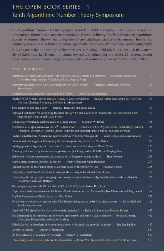
The Algorithmic Number Theory Symposium (ANTS), held biennially since 1994, is the premierinternational forum for research in computational number theory. ANTS is devoted to algorithmicaspects of number theory, including elementary, algebraic, and analytic number theory, thegeometry of numbers, arithmetic algebraic geometry, the theory of finite fields, and cryptography.

This volume is the proceedings of the tenth ANTS meeting, held July 9–13, 2012, at the Univer-sity of California, San Diego. It includes revised and edited versions of the 25 refereed paperspresented at the conference, together with extended abstracts of two of the five invited talks.

TABLE OF CONTENTS

1Deterministic elliptic curve primality proving for a special sequence of numbers — Alexander Abatzoglou,Alice Silverberg, Andrew V. Sutherland, and Angela Wong

21Imaginary quadratic fields with isomorphic abelian Galois groups — Athanasios Angelakis and PeterStevenhagen

41Iterated Coleman integration for hyperelliptic curves — Jennifer S. Balakrishnan

63Finding ECM-friendly curves through a study of Galois properties — Razvan Barbulescu, Joppe W. Bos, CyrilBouvier, Thorsten Kleinjung, and Peter L. Montgomery

87Two grumpy giants and a baby — Daniel J. Bernstein and Tanja Lange

113Improved techniques for computing the ideal class group and a system of fundamental units in number fields —Jean-François Biasse and Claus Fieker

135Conditionally bounding analytic ranks of elliptic curves — Jonathan W. Bober

145A database of elliptic curves over Q(√

5): a first report — Jonathan Bober, Alyson Deines, Ariah Klages-Mundt,Benjamin LeVeque, R. Andrew Ohana, Ashwath Rabindranath, Paul Sharaba, and William Stein

167Finding simultaneous Diophantine approximations with prescribed quality — Wieb Bosma and Ionica Smeets

187Success and challenges in determining the rational points on curves — Nils Bruin

213Solving quadratic equations in dimension 5 or more without factoring — Pierre Castel

235Counting value sets: algorithm and complexity — Qi Cheng, Joshua E. Hill, and Daqing Wan

249Haberland’s formula and numerical computation of Petersson scalar products — Henri Cohen

271Approximate common divisors via lattices — Henry Cohn and Nadia Heninger

295Explicit descent in the Picard group of a cyclic cover of the projective line — Brendan Creutz

317Computing equations of curves with many points — Virgile Ducet and Claus Fieker

335Computing the unit group, class group, and compact representations in algebraic function fields — KirstenEisenträger and Sean Hallgren

359The complex polynomials P(x) with Gal(P(x)− t)∼= M23 — Noam D. Elkies

369Experiments with the transcendental Brauer-Manin obstruction — Andreas-Stephan Elsenhans and Jörg Jahnel

395Explicit 5-descent on elliptic curves — Tom Fisher

413On the density of abelian surfaces with Tate-Shafarevich group of order five times a square — Stefan Keil andRemke Kloosterman

437Improved CRT algorithm for class polynomials in genus 2 — Kristin E. Lauter and Damien Robert

463Fast computation of isomorphisms of hyperelliptic curves and explicit Galois descent — Reynald Lercier,Christophe Ritzenthaler, and Jeroen Sijsling

487Elliptic factors in Jacobians of hyperelliptic curves with certain automorphism groups — Jennifer Paulhus

507Isogeny volcanoes — Andrew V. Sutherland

531On the evaluation of modular polynomials — Andrew V. Sutherland

557Constructing and tabulating dihedral function fields — Colin Weir, Renate Scheidler, and Everett W. Howe

AN

TS

X:

TenthA

lgorithmic

Num

berTheory

Symposium

How

e,KedlayaO

BS

1