iterative detection, decoding, and channel estimation in...

ABCDEFG

UNIVERS ITY OF OULU P.O.B . 7500 F I -90014 UNIVERS ITY OF OULU F INLAND

A C T A U N I V E R S I T A T I S O U L U E N S I S

S E R I E S E D I T O R S

SCIENTIAE RERUM NATURALIUM

HUMANIORA

TECHNICA

MEDICA

SCIENTIAE RERUM SOCIALIUM

SCRIPTA ACADEMICA

OECONOMICA

EDITOR IN CHIEF

PUBLICATIONS EDITOR

Professor Mikko Siponen

University Lecturer Elise Kärkkäinen

Professor Pentti Karjalainen

Professor Helvi Kyngäs

Senior Researcher Eila Estola

Information officer Tiina Pistokoski

University Lecturer Seppo Eriksson


Publications Editor Kirsti Nurkkala

ISBN 978-951-42-6219-7 (Paperback)ISBN 978-951-42-6220-3 (PDF)ISSN 0355-3213 (Print)ISSN 1796-2226 (Online)

U N I V E R S I TAT I S O U L U E N S I SACTAC

TECHNICA


TECHNICA

OULU 2010

C 358

Jari Ylioinas

ITERATIVE DETECTION, DECODING, AND CHANNEL ESTIMATION IN MIMO-OFDM

FACULTY OF TECHNOLOGY,DEPARTMENT OF ELECTRICAL AND INFORMATION ENGINEERING,UNIVERSITY OF OULU;CENTRE FOR WIRELESS COMMUNICATIONS,INFOTECH OULUUNIVERSITY OF OULU

C 358

ACTA

Jari Ylioinas

C358etukansi.kesken.fm Friday, May 14, 2010 1:28 PM

A C T A U N I V E R S I T A T I S O U L U E N S I SC Te c h n i c a 3 5 8

JARI YLIOINAS


Academic dissertation to be presented with the assent ofthe Faculty of Technology of the University of Oulu forpublic defence in Auditorium IT116, Linnanmaa, on 10June 2010, at 12 noon

UNIVERSITY OF OULU, OULU 2010

Copyright © 2010Acta Univ. Oul. C 358, 2010

Supervised byProfessor Markku Juntti

Reviewed byDocent Elena Simona LohanAssociate Professor Mark Reed

ISBN 978-951-42-6219-7 (Paperback)ISBN 978-951-42-6220-3 (PDF)http://herkules.oulu.fi/isbn9789514262203/ISSN 0355-3213 (Printed)ISSN 1796-2226 (Online)http://herkules.oulu.fi/issn03553213/

Cover designRaimo Ahonen

JUVENES PRINTTAMPERE 2010

Ylioinas, Jari, Iterative detection, decoding, and channel estimation in MIMO-OFDM Faculty of Technology, Department of Electrical and Information Engineering, University ofOulu, P.O.Box 4500, FI-90014 University of Oulu, Finland; Centre for WirelessCommunications, Infotech Oulu, University of Oulu, P.O.Box 4500, FI-90014 University ofOulu, FinlandActa Univ. Oul. C 358, 2010Oulu, Finland

AbstractIterative receiver techniques, multiple-input – multiple-output (MIMO) processing, andorthogonal frequency division multiplexing (OFDM) are amongst the key physical layertechnologies when aiming at higher spectral efficiency for a wireless communication system.Special focus is put on iterative detection, decoding, and channel estimation for a MIMO-OFDMsystem. After designing separately efficient algorithms for the detection, channel decoding, andchannel estimation, the objective is to optimize them to work together through optimizing theactivation schedules for soft-in soft-out (SfISfO) components.

A list parallel interference cancellation (PIC) detector is derived to approximate an a posterioriprobability (APP) algorithm with reduced complexity and minimal loss of performance. It isshown that the list PIC detector with good initialization outperforms the K-best list sphere detector(LSD) in the case of small list sizes, whereas the complexities of the algorithms are of the sameorder. The convergence of the iterative detection and decoding is improved by using a prioriinformation to also recalculate the candidate list, aside from the log-likelihood ratios (LLRs) ofthe coded bits.

Unlike in pilot based channel estimation, the least-squares (LS) channel estimator based onsymbol decisions requires a matrix inversion in MIMO-OFDM. The frequency domain (FD)space-alternating generalized expectation-maximization (SAGE) channel estimator calculates theLS estimate iteratively, avoiding the matrix inversion with constant envelope modulation. Theperformance and computational complexity of the FD-SAGE channel estimator are compared tothose of pilot based LS channel estimation with minimum mean square error (MMSE) post-processing exploiting the time correlation of the channel. A time domain (TD) SAGE channelestimator is derived to avoid the matrix inversion in channel estimation based on symbol decisionsfor MIMO-OFDM systems also with non-constant envelope modulation.

An obvious problem, with more than two blocks in an iterative receiver, is to find the optimalactivation schedule of the different blocks. It is proposed to use extrinsic information transfer(EXIT) charts to characterize the behavior of the receiver blocks and to find out the optimalactivation schedule for them. A semi-analytical expression of the EXIT function is derived for theLS channel estimator. An algorithm is proposed to generate the EXIT function of the APPalgorithm as a function of the channel estimate’s mutual information (MI). Surface fitting is usedto get closed form expressions for the EXIT functions of the APP algorithm and the channeldecoder. Trellis search algorithms are shown to find the convergence with the lowest possiblecomplexity using the EXIT functions. With the proposed concept, the activation scheduling canbe adapted to prevailing channel circumstances and unnecessary iterations will be avoided.

Keywords: activation scheduling, channel estimation, EXIT chart, iterative receiver, listdetection, MIMO, OFDM, SAGE

To my family

Preface

The research for this thesis has been carried out at the Centre for WirelessCommunications (CWC), University of Oulu, Finland. I want to thank ProfessorMatti Latva-aho, Dr. Ian Opperman, and Lic. Tech. Ari Pouttu, the directors ofCWC during my stay, for giving me the opportunity to work in such an energeticand inspiring working environment.

I am grateful to my supervisor Professor Markku Juntti for his invaluableguidance, scientific support, and especially encouragement during postgraduateresearch. I would like to thank Professor Tadashi Matsumoto for giving me ahint to study the activation scheduling of an iterative receiver, which becameone of the main topics of this thesis. I would like to express my gratitude to thereviewers of this thesis, Docent Elena Simona Lohan from Tampere University ofTechnology, Tampere, Finland and Associate Professor (Adjunct) Mark Reedfrom the Australian National University, Canberra, Australia. Their commentssignificantly improved the quality of the thesis. I am indebted to my line managerfrom my current employer Nokia Siemens Networks (NSN), Markku Vainikka,who has provided me with flexibility that has been needed in finalizing thisthesis. Samuli Kangaslampi is acknowledged for proofreading the manuscript.

The main part of the work presented in this thesis was carried out in theMIMO Techniques for 3G System and Standard Evolution (MITSE), Gain,and Beamforming and Radio Resource Management in Co-Operative WirelessNetworks (BeCON) projects. I would like to thank the project managers of theseprojects, Dr. Nenad Veselinovic and Lic. Tech. Visa Tapio, the technical steeringgroup members of the projects, as well as my colleagues in those projects. Inparticular, I would like to thank my office mates, regular lunch and ski-tripcompanions, and travelling companions, Dr. Giuseppe Abreu, Dr. MarianCodreanu, Giuseppe Destino, Jarkko Huusko, Dr. Umebayashi Kenta, Lic. Tech.Kai Kiiskilä, Petri Komulainen, Dr. Esa Kunnari, Davide Macagnano, CarlosMorais de Lima, Dr. Honglei Miao, Pedro Nardelli, Stefano Severi, HannaSaarela, Lic. Tech. Pirkka Silvola, Dr. Attaphongse Taparugssanagorn, Dr. AnttiTölli, Lic. Tech. Mikko Vehkaperä, and Qiang Xue for the refreshing momentsand fruitful discussions at the office and out there. The administrative support

7

of Antero Kangas, Elina Komminaho, Mari Lehmikangas, Sari Luukkonen, KirsiOjutkangas, Hanna Saarela, Jari Sillanpää, Tero Suutari, and Timo Äikas ishighly appreciated. Special thanks go to my co-authors Juha Karjalainen, Dr.Raghavendra Madanahally, Markus Myllylä, and Samuli Tiiro as well as MarkkuJokinen for the fruitful co-operation.

The research for this thesis has been financially supported by Infotech OuluGraduate School during the years 2008-2009. Funding through the projectswas provided by the Finnish Funding Agency for Technology and Innovation,Elektrobit, Nokia, Nokia Siemens Networks, Texas Instruments, Uninord, and theAcademy of Finland, which is gratefully acknowledged. I was privileged to receivepersonal grants for Doctoral studies from the following Finnish foundations:Tekniikan edistämissäätiö, Telealan edistämissäätiö, Tauno Tönningin säätiö,Oulun yliopiston tukisäätiö, Nokia Oyj:n säätiö, and HPY:n tutkimussäätiö.These acknowledgements encouraged me to go on with my research work andthey are gratefully recognized.

During the years the research for this thesis was carried out I was fortunateto be involved with the following groups. The rehearsals, gigs, parties, andthe wonderful people in Cassiopeia, the mixed choir of the University of OuluStudents’ Union, helped me to forget the research problems when needed. Also,the rehearsals, recording sessions, and gigs with Bedtime Acoustics were a lotof fun and great counter balance. The football teams, Supertele, Jalopenos,and Tuurihaukat helped me to stay in quite good form and, thus, helped mestay concentrated on research. For all the friends, who are too numerous to beacknowledged individually, thank you for the midsummer parties, barbecuingparties, sauna evenings, trips, and other shared moments. I needed those!

My deepest gratitude goes to my parents Eija and Kauko, for their love,support, and encouragement towards education. The help you have given duringmy life is invaluable. I wish to thank my sister Jaana and brother Juha forlifelong friendship and help. Many thanks go to the companions of my sister andbrother, Tomi and Piia, and to my family-in-law, Eile, Mauri, Minttu, Lari, andAnne, for the moments we have shared.

My warmest thanks belong to my wife Pihla for her love, support, and theunderstanding she has for me, and to our son Aapo for just being there andbringing the sunshine into our life. I know that I demanded a lot. Swapping to a

8

new job, starting the house building project, moving to a new apartment, andfinalizing this thesis at the same time created hectic times in our life.

Oulu, May 9, 2010 Jari Ylioinas

9

Symbols and abbreviations

ak state at activation kb(n) bit vector after the channel encoder and interleaving at time

instant n, (McMtP × 1)

bmc,mt,p(n) bit mapped to the mcth bit position at the mtth transmit antennaand the pth subcarrier

b bit vector which is the part of b transmitted from the transmitantennas over one subcarrier, (MtMc × 1)

b [q] subvector of b obtained by omitting its qth element, (MtMc−1×1)

C r receive antenna correlation matrix, (Mr ×Mr)

C t transmit antenna correlation matrix, (Mt ×Mt)

C tr antenna correlation matrix, (MtMr ×MtMr)

Ec expected power of the constellationEs symbol energy received by a receive antennaF truncated DFT matrix, (P × L)

F block diagonal matrix having truncated DFT matrices on itsdiagonal, (MtP ×MtL)

fd Doppler frequencyGLMMSE LMMSE filtering matrix in detection, (Mr ×Mt)

hmrtime domain channel vector containing the channels between thetransmit antennas and the mrth receive antenna, (MtL× 1)

hmt,mrtime domain channel vector containing the channel between themtth transmit antenna and the mrth receive antenna, L× 1

hmt,mr,llth multipath component between the mtth transmit and themrth receive antenna

H p frequency domain MIMO channel for the pth subcarrier, (Mr×Mt)

hmt the mtth column of the frequency domain channel matrix H ,(Mt × 1)

IN identity matrix, N ×NK number of candidates in LL length of the channel impulse responseLA1 a priori information in the input of the detector

11

LA2 a priori information in the input of the decoderLCP length of the cyclic prefixLD1 a posteriori information in the output of the detectorLD2 a posteriori information in the output of the decoderLE1 extrinsic information given by the detectorLE2 extrinsic information given by the decoderlA1 vector of all LA1 values corresponding to one subcarrier (MtMc×1)

lA1,[q] vector of all LA1 values corresponding to one subcarrier, omittingbq, (MtMc − 1× 1)

L list of candidate symbol vectorsMA a priori mutual informationMc number of bits per constellation pointmc bit position indexMD convergence targetME extrinsic mutual informationMr number of receive antennasmr receive antenna indexMt number of transmit antennasmt transmit antenna indexN0 power spectral density of noiseNi number of iterationsNP number of preambles in a block of OFDM symbolsNsymb number of OFDM symbols in the blockn time indexomt,mr,l component of the time domain received signal at the mrth receive

antenna transmitted by themtth transmit antenna and propagatedthrough the lth path, (P × 1)

P number of subcarriersp subcarrier indexpk specific activation schedule including k activationsTB duration of OFDM symbolT dec decoder EXIT functionT det detector EXIT functionTh channel estimator EXIT functionv metric vector associated with a scheduling path

12

vmt,mr,l(n) Wiener filtering vectorwmr

noise vector containing samples from a complex zero-mean whiteGaussian noise process with covariance σ2wI P , (P × 1)

wp noise vector containing samples from a complex zero-mean whiteGaussian noise process, (Mr × 1)

wmr time domain noise vector containing samples from a complexzero-mean white Gaussian noise process, (P × 1)

X matrix containing the transmitted symbols from all the transmitantennas and subcarriers, (P ×MtP )

Xmt matrix containing the transmitted symbols from themtth transmitantenna and all subcarriers on its diagonal, (P × P )

xmt(n) symbol vector transmitted from the mtth transmit antenna at

time instant n, (P × 1)

xmt,p(n) symbol transmitted from the mtth transmit antenna at the pthsubcarrier at time instant n

x p symbol vector transmitted over the transmit antennas at the pthsubcarrier, (Mt × 1)

xmt,l time domain signal from the mtth transmit antenna , (P × 1)

ymr

(n) received signal at the receive antenna mr at time instant n, (P ×1)

ymr,p received signal at the receive antenna mr and subcarrier pyp received signal on the pth subcarrier over the receive antennas,

(Mr × 1)

ymrtime domain received signal at the receive antenna mr, (P × 1)

zmt component of the received signal transmitted from the mtthtransmit antenna through the channel hmt and corrupted by thenoise, (Mr × 1)

zmt,mr component of the received signal at the mrth receive antennatransmitted by the mtth transmit antenna, (P × 1)

Ω set of complex constellation pointsρrmr,m′r

spatial correlation coefficient between the receive antennas mr

and m′rΣa(n),a(n′) autocorrelation of random variable aΣa,b cross-covariance vector between the random variable a and the

random vector b

13

Σa autocovariance matrix of the random vector aσ2wI P covariance of the noise vector wmr

ρtmt,m′t

spatial correlation coefficient between the transmit antennas mt

and m′tρmt,mr(n− n′)temporal correlation function of the channel impulse response

taps〈a, b〉 correlation coefficient between a and b[A]l the lth column of matrix A|S| cardinality of set S‖ · ‖ Euclidean norm(·)H Hermitean transpose of the argument(·)T transpose of the argument(·)∗ complex conjugate of the argument(·) estimate of the argument(·) soft estimate of the argument in the context of detection⊗ the Kronecker product elementwise vector multiplicationE(·) expectation of the argumentJ(·) J-functionJ0(·) the zeroth-order Bessel function of the first kindPr(·) probability of the argument to occurp(·) probability density functionln(·) natural logarithm of the argumentlog2(·) logarithm of the argument in base 2M(·) Gray mappingmin(·) minimumQ(·) integral of the tail of a zero-mean Gaussian PDF with a variance

of onetanh(·) hyperbolic tangent of the argumentBq,±1 the sets of 2MtMc possible bit vectors b with bq = ±1

Cm×n set of m× n complex matricesIN set of natural numbersPk set of surviving pathsPk,n set of surviving paths entering state nIRm×n set of m× n real matrices

14

IR+ set of positive real numbersSP preamble symbol index setVk set of metrics of surviving pathsVk,n set of metrics of surviving paths entering state n≈ approximative equal

1G the first generation2G the second generation3G the third generation3GPP the third generation partnership project4G the fourth generation16QAM 16 point quadrature amplitude modulation64QAM 64 point quadrature amplitude modulationAMSE analytical mean square errorAoA angle of arrivalAoD angle of departureAPP a posteriori probabilityAWGN additive white Gaussian noiseBeFS best-first searchBICM bit-interleaved coded modulationBrFS breadth-first searchCC constituent codeCDMA code division multiple accessCFO carrier frequency offsetCFR channel frequency responseCIR channel impulse responseCP cyclic prefixCRLB Cramer-Rao lower boundCSI channel state informationDA data aidedDD decision directedDFS depth-first searchDFT discrete Fourier transformE expectationED Euclidean distance

15

EDGE Enhanced Data Rates for GSM EvolutionEM expectation-maximizationETSI European Telecommunications Standards InstituteEXIT extrinsic information transferFD frequency domainFDD frequency division duplexFDMA frequency division multiple accessFER frame error rateFFT fast Fourier transformFPGA field-programmable gate arrayFSD fixed complexity sphere decoderGI global iterationGPRS Generalized Packet Radio ServiceGSM Global System for Mobile communicationsHSPA High Speed Packet AccessIFFT inverse fast Fourier transformIBI inter-block interferenceICI inter-carrier interferenceICT information and communication technologyIMT-A International Mobile Telecommunications-AdvancedIR-LSD increasing radius list sphere detectorIR-SD ever-increasing radius sphere detectorISI inter-symbol interferenceITU International Telecommunication UnionLDPC low-density parity-checkLLR log-likelihood ratioLMMSE linear minimum mean square errorLTE long-term evolutionLTE-A Long-Term Evolution-AdvancedLS least-squaresLSD list sphere detectorM maximizationMAP maximum a posteriori probabilityMC multicarrierMFS metric-first search

16

ML maximum likelihoodMI mutual informationMIMO multiple-input multiple-outputMMSE minimum mean square errorMSE mean square errorOFDM orthogonal frequency division multiplexingOFDMA orthogonal frequency division multiple accessOSIC ordered successive interference cancellationPACE pilot aided channel estimationPAPR peak-to-average power ratioPAS power azimuth spreadPCCC parallel concatenated convolutional codePDF probability density functionPDP power delay profilePIC parallel interference cancelationRA repeat-accumulateRX receiverSAGE space alternating generalized expectation-maximizationSD sphere detectionSDR semidefinite relaxationSfISfO soft-in soft-outSIC successive interference cancellationSINR signal-to-noise-plus-interference ratioSISO single-input single-outputSM spatial multiplexingSNR signal-to-noise ratioSTBC space-time block codeSTC space-time codingSTTC space-time trellis codeTD time domainTDD time division duplexTU typical urbanTX transmitterUMTS Universal Mobile Telecommunication SystemQoS quality of service

17

QPSK quadrature phase shift keyingQRD QR decompositionTDMA time division multiple accessV-BLAST vertical Bell Labs Layered Space-TimeWLAN wireless local area networkWiMAX Worldwide Interoperability for Microwave AccessWMAN wireless metropolitan area networkZF zero-forcing

18

Contents

AbstractPreface 7Symbols and abbreviations 11Contents 191 Introduction 21

1.1 Evolution of mobile communication systems. . . . . . . . . . . . . . . . . . . . . . . . .211.2 MIMO-OFDM – the key technology . . . . . . . . . . . . . . . . . . . . . . . . . . . . . . . . 221.3 Aims, outline, and contribution of the thesis . . . . . . . . . . . . . . . . . . . . . . . . 25

2 Literature review 312.1 Channel estimation in wireless OFDM systems . . . . . . . . . . . . . . . . . . . . . . 31

2.1.1 Data aided methods . . . . . . . . . . . . . . . . . . . . . . . . . . . . . . . . . . . . . . . . . .322.1.2 Decision directed methods. . . . . . . . . . . . . . . . . . . . . . . . . . . . . . . . . . . .34

2.2 MIMO detection . . . . . . . . . . . . . . . . . . . . . . . . . . . . . . . . . . . . . . . . . . . . . . . . . . . .342.2.1 Linear detection and non-linear improvements . . . . . . . . . . . . . . . . 352.2.2 Optimal detection and its approximations . . . . . . . . . . . . . . . . . . . . 36

2.3 Iterative detection, decoding, and channel estimation . . . . . . . . . . . . . . . 383 Preliminaries 43

3.1 Model for received signal . . . . . . . . . . . . . . . . . . . . . . . . . . . . . . . . . . . . . . . . . . . 433.2 MIMO channel model . . . . . . . . . . . . . . . . . . . . . . . . . . . . . . . . . . . . . . . . . . . . . . 443.3 Iterative detection and decoding . . . . . . . . . . . . . . . . . . . . . . . . . . . . . . . . . . . . 45

4 Detection of spatially multiplexed signals in MIMO-OFDM 474.1 Linear minimum mean square algorithm . . . . . . . . . . . . . . . . . . . . . . . . . . . . 474.2 List parallel interference cancellation algorithm . . . . . . . . . . . . . . . . . . . . . 484.3 List re-calculation in iterative detection and decoding . . . . . . . . . . . . . . . 524.4 Numerical examples . . . . . . . . . . . . . . . . . . . . . . . . . . . . . . . . . . . . . . . . . . . . . . . . 53

4.4.1 Results with 2 × 2 antenna configuration. . . . . . . . . . . . . . . . . . . . .544.4.2 Results with 4 × 4 antenna configuration. . . . . . . . . . . . . . . . . . . . .584.4.3 Complexity Comparisons . . . . . . . . . . . . . . . . . . . . . . . . . . . . . . . . . . . . . 60

4.5 Summary and discussion. . . . . . . . . . . . . . . . . . . . . . . . . . . . . . . . . . . . . . . . . . . .625 Channel estimation for MIMO-OFDM system 65

5.1 Iterative receiver with channel estimator . . . . . . . . . . . . . . . . . . . . . . . . . . . . 65

19

5.2 Least squares algorithm. . . . . . . . . . . . . . . . . . . . . . . . . . . . . . . . . . . . . . . . . . . . .675.3 Frequency domain space-alternating generalized expectation

maximization algorithm . . . . . . . . . . . . . . . . . . . . . . . . . . . . . . . . . . . . . . . . . . . . 685.4 Time domain space-alternating generalized expectation

maximization algorithm . . . . . . . . . . . . . . . . . . . . . . . . . . . . . . . . . . . . . . . . . . . . 695.5 Minimum mean square error algorithm . . . . . . . . . . . . . . . . . . . . . . . . . . . . . 705.6 Complexity comparison between LS, SAGE, and MMSE

channel estimators . . . . . . . . . . . . . . . . . . . . . . . . . . . . . . . . . . . . . . . . . . . . . . . . . . 715.7 Implementation aspects of LS, SAGE, and MMSE channel

estimators . . . . . . . . . . . . . . . . . . . . . . . . . . . . . . . . . . . . . . . . . . . . . . . . . . . . . . . . . . 735.7.1 LS estimator architecture . . . . . . . . . . . . . . . . . . . . . . . . . . . . . . . . . . . . 735.7.2 SAGE estimator architecture . . . . . . . . . . . . . . . . . . . . . . . . . . . . . . . . . 765.7.3 MMSE filter implementation . . . . . . . . . . . . . . . . . . . . . . . . . . . . . . . . . 79

5.8 Numerical examples . . . . . . . . . . . . . . . . . . . . . . . . . . . . . . . . . . . . . . . . . . . . . . . . 815.8.1 Comparison of channel estimation algorithms. . . . . . . . . . . . . . . . .825.8.2 Comparison of soft MIMO detection algorithms with

estimated channel . . . . . . . . . . . . . . . . . . . . . . . . . . . . . . . . . . . . . . . . . . . . 905.9 Summary and discussion. . . . . . . . . . . . . . . . . . . . . . . . . . . . . . . . . . . . . . . . . . . .95

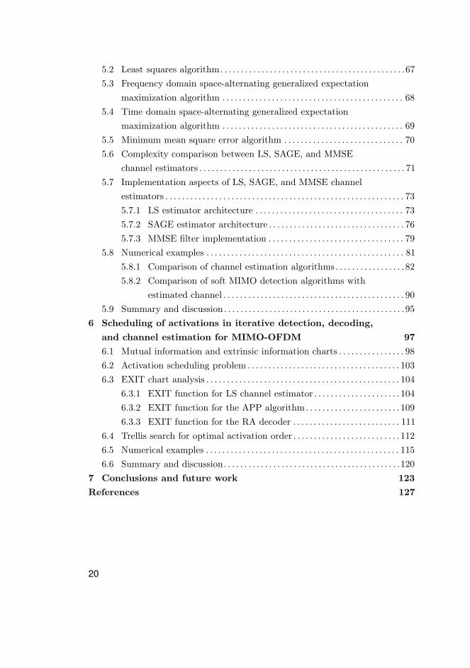
6 Scheduling of activations in iterative detection, decoding,and channel estimation for MIMO-OFDM 976.1 Mutual information and extrinsic information charts . . . . . . . . . . . . . . . . 986.2 Activation scheduling problem . . . . . . . . . . . . . . . . . . . . . . . . . . . . . . . . . . . . . 1036.3 EXIT chart analysis . . . . . . . . . . . . . . . . . . . . . . . . . . . . . . . . . . . . . . . . . . . . . . . 104

6.3.1 EXIT function for LS channel estimator . . . . . . . . . . . . . . . . . . . . . 1046.3.2 EXIT function for the APP algorithm. . . . . . . . . . . . . . . . . . . . . . . 1096.3.3 EXIT function for the RA decoder . . . . . . . . . . . . . . . . . . . . . . . . . . 111

6.4 Trellis search for optimal activation order . . . . . . . . . . . . . . . . . . . . . . . . . . 1126.5 Numerical examples . . . . . . . . . . . . . . . . . . . . . . . . . . . . . . . . . . . . . . . . . . . . . . . 1156.6 Summary and discussion. . . . . . . . . . . . . . . . . . . . . . . . . . . . . . . . . . . . . . . . . . .120

7 Conclusions and future work 123References 127

20

1 Introduction

During the last decades, we have witnessed a swift evolution of wireless com-munication systems and standards. From the first generation (1G) analogsystems supplying only voice services, the standards evolved through the secondgeneration (2G) systems to the third generation systems (3G). Both the 2G and3G systems are digital systems offering data services besides the voice. Theparticular driving force for this fast evolution are the ever increasing data raterequirements for wireless communication systems. Consequently, standardizationand research programs are currently working with the evolution of 3G, aiming atfourth generation (4G) systems.

The radio spectrum is crowded, which makes it challenging to respond to theincreasing data rate demands. Evidently, when additional spectrum is scarce, ithas to be used more efficiently. This thesis concentrates on developing advancedreceiver algorithms to improve spectral efficiency. Special focus is put on iterativedetection, decoding, and channel estimation to reduce the overhead requiredby conventional receiver algorithms. In Section 1.1, the evolution of mobilecommunication systems is discussed in more detail. The key technologies toimprove the performance of wireless communication systems are introduced inSection 1.2. Section 1.3 presents the aims and outline of the thesis. Finally, theauthor’s contribution to the original publications is summarized in Section 1.3.

1.1 Evolution of mobile communication systems

Due to the poor spectral efficiency of 1G analog systems and the rapid growthin the number of cellular users, operators were driven to invest in 2G digitalsystems, such as the Global System for Mobile communications (GSM) [17, 18].The GSM specifications were developed by the European TelecommunicationsStandards Institute (ETSI) [19]. The 2G systems were mainly designed forvoice services, offering only low data rate capabilities [20]. To improve the datarates of GSM networks, the Generalized Packet Radio Service (GPRS) andEnhanced Data Rates for GSM Evolution (EDGE) were introduced. However,these extensions only temporarily satisfied the hunger for data services.

21

Different services have different quality of service (QoS) requirements. Forexample, voice services require low delay using only low data rates, while webbrowsing causes a bursty transmission requiring high peak data rates. Thesedemands were taken into consideration when designing 3G systems, such asthe Universal Mobile Telecommunication System (UMTS) [21]. UMTS and itsevolution High Speed Packet Access (HSPA) were defined in the third generationpartnership project (3GPP) [22]. The Long-Term Evolution (LTE) of 3G [23, 24]has been under study in 3GPP as well. The peak data rate targets set forthe LTE system are 100 Mbit/s for downlink and 50 Mbit/s for uplink whenoperating in 20 MHz spectrum allocation. An optional path towards higher datarates is offered by solutions like wireless local- or metropolitan-area networks(WLAN, WMAN) [25, 26] with increased capacity and coverage, as well as byWorldwide Interoperability for Microwave Access (WiMAX) [27] with improvedsupport for mobility and QoS. The International Mobile Telecommunications-Advanced (IMT-A) concept created by the International TelecommunicationUnion (ITU) sets the requirements beyond 3G, also referred to as 4G radioaccess. LTE-Advanced (LTE-A) [28] is being developed by 3GPP to meet therequirements set by IMT-A. LTE-A is aiming up at peak data rates of 1Gbit/sin downlink and 500 Mbit/s in uplink.

1.2 MIMO-OFDM – the key technology

Spectral sharing among the users, also referred to as multiple access, is carriedout by dividing the signaling dimensions along the time, code, and/or frequencydomains [29]. In time division multiple access (TDMA), the users are givenorthogonal time slots, and each user occupies the entire frequency band overthe assigned time slot. The GSM networks are based on TDMA. The users areseparated by orthogonal codes in code division multiple access (CDMA). Thespectrum sharing of the UMTS system is based on CDMA. In frequency divisionmultiple access (FDMA), the total system bandwidth is divided into orthogonalfrequency channels. Orthogonal frequency division multiple access (OFDMA)combines orthogonal frequency division multiplexing (OFDM) and FDMA and isone of the multiple access candidates for beyond 3G systems.

OFDM is a special form of multicarrier (MC) transmission, which was firstproposed by Chang [30] in 1966. What is known as OFDM today, was proposed

22

by Weinstein and Ebert [31] in 1971 and was first applied to wireless mobilecommunications by Cimini [32] in 1985. In OFDM, the transmitted data ismodulated via an inverse fast Fourier transform (IFFT) block and demodulatedwith a fast Fourier transform (FFT) block at the receiver.

One of the rewards of OFDM is the simplicity with which the receiver canprocess channel impairments. In a radio channel, time-varying fading corruptsthe transmitted signals [17, 20, 29, 33]. The time-varying fading can in factbe divided into large-scale fading and small-scale fading. The motion of amobile user over large geographical areas causes changes in the average pathloss, resulting in large-scale fading. Large-scale fading is usually modeled withan experimental model [34]. Small-scale fading is caused by an order of half awavelength changes in the position of the receiver resulting in fast changes in thesignal level. These changes are due to signals propagated over multiple pathsand then summing up at the receiver. Multipath propagation also results infrequency selective fading, incuring inter-symbol interference (ISI). OFDM turnsa frequency selective channel into a set of parallel flat fading channels, and, thus,avoids the use of equalizers in ISI mitigation. This significantly simplifies thereceiver design compared to conventional single carrier systems like 2G and 3G,in which channel equalizers are used in ISI mitigation [12–16, 35]. An essentialtechnique in OFDM is the use of a cyclic prefix (CP) which is longer than themaximum excess delay of the channel in between adjacent OFDM blocks toavoid inter-block interference (IBI) [36, 37].

OFDM provides an opportunity to use link adaptation, including the adap-tation of the transmission power or data rate of each subchannel. Thus, thewater-filling principle [38] can be applied to assist in achieving higher data rates.Water-filling dates back to Shannon [39]. The highest data rate can be achievedfor frequency selective channels by using a MC system with an infinitely dense setof subchannels and adapting the transmission powers and data rates accordingto the signal-to-noise ratio (SNR) on different subchannels.

OFDM brings with it some drawbacks besides the rewards. OFDM is sensitiveto synchronization errors. In particular, an error in frequency synchronizationcauses inter-carrier interference (ICI). Another problem with OFDM is the largepeak-to-average power ratio (PAPR), which challenges the requirements forpower amplifier design. More details about these drawbacks and OFDM ingeneral can be found in [40] and the references therein.

23

Multiple-input multiple-output (MIMO) processing [41, 42] exploits multipleantenna elements at the transmitting end as well as at the receiving end. Themain idea in MIMO systems is space-time signal processing, where time andspace domain signals are jointly processed. MIMO systems can be seen as anextension of conventional smart antenna systems. Those systems employ multipleantenna elements at only the transmitter or the receiver for beamforming orspatial diversity. Beamforming increases the average SNR by focusing the energyin the desired directions using correlated antenna elements. On the other hand,the correlation of antenna elements should be minimized when link reliabilityis improved by spatial diversity schemes. More details on smart antenna andMIMO techniques can be found in [43, 44].

The benefits of antenna arrays are retained in MIMO processing. Actually,the advantage of the MIMO system is far beyond what just an array or diversitygain can achieve due to the underlying matrix that MIMO uses instead of thevector channel for antenna arrays. The potential of a tremendous capacityincrease by using MIMO processing was reported in [45, 46]. However, accordingto [41], the first hints of the capacity gains of MIMO processing were publishedby Winters in [47]. To maximize the data rate in [48–50], the vertical Bell LabsLayered Space-Time (V-BLAST), also referred to as spatial multiplexing (SM),was introduced and it was shown to be capable of transmitting min(MT,MR)independent data streams over the MIMO system with MT transmit and MR

receive antennas, provided that the channel matrix is full rank. The separationof the data streams at the receiver is based on rich multipaths. Thus, MIMOsystems effectively exploit multipath propagation instead of trying to mitigate itlike conventional antenna array systems.

The concept of space-time coding (STC) pursues diversity gain from theMIMO channel. The major advancement in the field of STC was the reportingof space-time trellis codes (STTC) in [51]. These codes give a diversity benefitequal to the number of transmit antennas and coding gain that depends onthe complexity of the code. The decoding complexity was the drawback ofSTTC since it is performed by a multidimensional Viterbi algorithm. Thespace-time block codes (STBC) [52], originally for two transmit antennas, solvedthe problem of decoding complexity by requiring only simple linear processing inthe decoding. STBC was generalized to an arbitrary number of antennas in

24

[53]. As may be expected, it is possible to establish a tradeoff between data ratemaximization through SM and diversity maximization through STC [54, 55].

The MIMO techniques discussed above are developed for flat fading channels.However, many of the current and future wireless communication systems arebroadband in nature, i.e., the communication is over a frequency selectivechannel. Consequently, OFDM, which turns the frequency selective channel intomultiple parallel flat fading channels, is a very promising companion for MIMOprocessing, resulting in so called MIMO-OFDM [56–59]. MIMO-OFDM hasbeen selected to be the air interface of several standards, such as 3G LTE [60],LTE-Advanced [61] and WiMAX [26].

1.3 Aims, outline, and contribution of the thesis

The aim of this thesis in a broad sense is to develop receiver algorithms whichenable more efficient use of radio spectrum. This is motivated by the fact thatradio spectrum is a limited resource and, thus, to serve the increasing needs,the spectrum has to be used more efficiently. Secondly, more efficient use ofspectrum also helps to improve power efficiency. This assists in reducing carbonemissions, that has become important in recent years. The information andcommunication technologies (ICTs) sector contributes between 2-2.5 per cent ofgreenhouse gases [62]. As the ICT sector is growing faster than the rest of theeconomy, it is likely that this share will increase in future. The topics consideredin this thesis do not alone solve the issue, but other means are required as well.

The modulation techniques widely accepted for future wireless communicationsystems such as MIMO processing and an OFDM air interface have been takenas working assumptions also in this thesis, since they improve spectral efficiency.However, any standard is not strictly followed but used more as a guideline inorder not to limit the possibilities to improve spectral efficiency. There are amultitude of functions that a receiver has to perform in wireless communicationand they have an impact on spectral efficiency. However, the special focus in thisthesis was to use the very basic functions such as detection, channel decoding,and channel estimation.

The optimal joint detection/decoding receiver is the technique that leads tothe most efficient use of spectrum. Unfortunately, for systems with practicalchannel coding, the complexity is intractable. The turbo principle has been

25

shown to be an efficient way to approximate the optimal receiver performanceand is studied in this thesis. The most efficient way to process the signal receivedfrom the channel would be the a posteriori probability (APP) algorithm. Sinceit becomes computationally intensive with multiple transmit antennas and withhigher order modulations, ways to approximate the APP algorithm are takeninto consideration. Naturally, the effects of detector approximation on the turboprinciple applied between the soft MIMO detector and a channel decoder are afocus of this thesis.

Conventionally, channel estimation is based on known reference signals.However, these reference signals consume resources from the actual user dataand, thus, decrease the spectral efficiency of wireless systems. The approachtaken in this thesis is to look for means to minimize the resources given forreference signals by using the user data for estimation purposes. Thus, this isthe part of the thesis which is the most different from conventional thinkingwithin standard receiver systems. The iterative channel estimation algorithmssuite turbo processing and they are studied in this thesis.

One of the objectives of this work is to use separately efficient algorithms fordetection, channel decoding, and channel estimation and to optimize them towork together. With iterative algorithms in cases with more than two blocks,the question of optimal activation scheduling arises to achieve the convergencewith minimal complexity. Naturally, to fully optimize the transmission, thechannel state is known at the transmitter and then the transmission can beoptimized to the channel state; however, in this thesis, the transmitter is notassumed to know the channel information.

Chapter 2 presents literature review of previous and parallel work relatedto the contributions of the thesis. The review includes the channel estimationmethods and the detection methods discussed in the literature in the contextof OFDM systems. The topic of iterative detection, decoding, and channelestimation is reviewed as well.

Chapter 3 contains the signal and channel models for the MIMO-OFDMsystem. Rayleigh distributed channels are assumed in this thesis, since MIMOprocessing relies on the presence of rich multipath. However, the algorithmsstudied in this thesis are not limited to be used only in Rayleigh distributedchannels. The concepts of iterative detection and decoding are also presented.

26

Chapter 4 focuses on the MIMO detection part of the iterative receiver.Perfect channel information is assumed to be available at the receiver. The resultshave been presented in part in [1, 5–7]. The contributions of this chapter are asfollows. A new list detector named the list parallel interference cancellation (PIC)detector is derived. The list PIC algorithm was originally presented in [5]. Theperformance of the list PIC detector is studied with different modulation methodsand antenna configurations. Its performance and complexity are compared tothe important list sphere detection algorithms discussed in the literature. Thesecomparisons are also available in [7]. The chapter illustrates how convergence ofthe iterative detection and decoding can be accelerated by re-calculating thecandidate list besides the log-likelihood ratio (LLR) values which was shownoriginally in [6].

Chapter 5, which has been published in part in [1, 4, 8, 9], considerschannel estimation for a MIMO-OFDM system. The least-squares (LS) channelestimation algorithm is reviewed and its intensive computational requirements indecision directed (DD) mode are pointed out. The frequency domain (FD) spacealternating generalized expectation-maximization (SAGE) channel estimationalgorithm is given as a solution to reduce the computational complexity inthe case of constant envelope constellations in DD mode. Minimum meansquare error (MMSE) channel estimation is reviewed here as well. The originalcontributions of this chapter are as follows. The inefficiency of the FD-SAGEalgorithm in the case of non-constant envelope constellations is pointed out.This was first presented in [1]. The time domain (TD) SAGE channel estimationalgorithm originally proposed in [4] is derived to solve the complexity issuealso with higher order constellations. The implementation aspects of the LS,FD-SAGE, and MMSE channel estimators are considered by presenting possiblearchitecture designs for them. These results can also be found from [8, 9]. Theperformance of the channel estimation algorithms is studied in various scenarios.

Chapter 6 is included in part in [2, 3] and presents a framework for theactivation scheduling of a soft MIMO detector, a channel decoder, and a channelestimator. The framework is based on extrinsic information transfer (EXIT)chart analysis. Trellis search algorithms are shown to find the activation schedulewhich guarantees convergence with minimal complexity if there is an openingbetween the EXIT functions of the detector, the decoder, and the channelestimator. The main original contributions of the chapter are as follows. A

27

semi-analytical method to generate the EXIT function for the LS channelestimator in MIMO-OFDM systems is derived. The derivation is based on theassumption that the multipath channel between each antenna pair is consideredas a set of parallel channels with colored Gaussian noise. An algorithm isproposed to generate the EXIT function for the soft MIMO detector as a functionof the mutual information between the channel estimate and the true channelstate.

Chapter 7 concludes the thesis. The main results and conclusions aresummarised. Furthermore, some questions remaining open and directions forfuture research are discussed.

The author’s contribution to the publications

This thesis is written as a monograph for the sake of clarity, but it is based onnine original publications that have been published, accepted for publication, orsubmitted to a journal. The author was the main contributor for [1–8], anddeveloped the main ideas and all the results in them. The other authors providedideas, comments, help, and in the case of [8], the second author provided somesimulation results. In [9], the author provided help, guidance, and ideas to thefirst author.

All simulation software for the numerical results was produced by the author,with the following exceptions. All results with turbo codes, have used turboencoding and decoding software by Lic. Tech. Mikko Vehkaperä. All simulatedchannels were produced with the channel simulator by Dr. Esa Kunnari. Therepeat accumulate encoder and decoder software used in Chapter 6 as well asthe function calculating numerically the mutual information based on histogrammeasurements were implemented by Mr. Juha Karjalainen. The K-best andincreasing radius (IR) list sphere detection (LSD) software were implemented byMr. Markus Myllylä and the MMSE post-prosessing filter for channel estimationwas implemented by Dr. Honglei Miao.

In [5], the list PIC detector was derived. The list PIC detector was applied asa soft MIMO detector in a receiver performing iterative detection, decoding, andchannel estimation in [6]. In addition, the list re-calculation was proposed in [6]to accelerate the convergence. The performance and complexity of the list PICdetector was compared to important LSD algorithms in [7]. The main results of

28

[5–7] were collected together and presented in [1]. In addition, the inefficiency ofthe FD-SAGE algorithm in the case of non-constant envelope constellationswas pointed out in [1]. In [4], the TD-SAGE channel estimation algorithm wasderived to solve the complexity issue of the FD-SAGE algorithm with higherorder constellations. The implementation aspects of the LS, FD-SAGE, andMMSE channel estimators were considered by presenting possible architecturedesigns for them in [8, 9]. Finally, the framework for activation scheduling of asoft MIMO detector, a channel decoder, and a channel estimator was presentedin [3]. A semi-analytical method to generate the EXIT function for the LSchannel estimator in MIMO-OFDM systems was derived and an algorithmwas proposed to generate the EXIT function for the soft MIMO detector as afunction of the mutual information between the channel estimate and the truechannel state. The topic of [3] was then more extensively covered in [2].

Applicability for commercial MIMO-OFDM systems

The results presented in Chapter 4 are applicable for current and plannedcommercial systems based on MIMO-OFDM. The list PIC algorithm performsthe detection of each subcarrier separately, being easily scalable for any numberof subcarriers. The iterative detection and decoding discussed in Chapter 4scales easily as well with different system parameters. However, the latencymight set a constraint for the number of iterations with iterative detection anddecoding.

There is no restriction to apply the algorithms discussed in Chapter 5 incurrent and planned commercial systems based on MIMO-OFDM. However, oneshould note that many of the results presented in the chapter assume lowerpilot density than the ones used in systems at present. Consequently, the gainusing the decoded data in estimation would be smaller with systems havinghigher reference signal density. On the other hand, due to the increasing needsof wireless data, the spectrum has to be used more efficiently. Furthermore,to lower the share of greenhouse gases produced by the ICT sector, the powerefficiency has to be improved as well. These things give motivation to reduce thereference signal density and at the same time motivation to use the algorithmsdiscussed in Chapter 5.

29

The concept of activation scheduling considered in Chapter 6 is based onEXIT analysis assuming extremely long code blocks. The applicability of theconcept for more realistic block lengths used in real systems is left for futurestudies. The results as such cannot be used, but they rather give a hint that thescheduling of the activations might bring some gain in performance and savingsin complexity if the receiver has more than two SfISfO components.

30

2 Literature review

A review of the existing literature and parallel work related to the scope of thisthesis is provided in this chapter. Section 2.1 reviews channel estimation methodsfor OFDM systems, concentrating on data aided and decision directed methodscovering the basic linear algorithms and including some non-linear improvementsas well as the most important approximations of the optimal detection. Section 2.2provides a survey on MIMO detection literature. Finally, literature consideringiterative receiver algorithms and especially iterative detection, decoding, andchannel estimation algorithms is presented in Section 2.3. This section alsocovers the EXIT chart analysis literature related to the scope of this thesis.

2.1 Channel estimation in wireless OFDM systems

The principle of synchronized (coherent) detection [63] is mainly used in theexisting wireless communication systems. In other words, the channel state isestimated and the estimate is used in the detection and decoding as if it wasthe true channel state. Channel estimation can be avoided by using differentialmodulation techniques. However, this would limit the data rate and cause adrop in the performance [64, 65]. Another possibility, especially in systems withtime division duplex (TDD) but also with frequency division duplex (FDD) [66],is to perform channel estimation at the base station and send a pre-distortedsignal to the mobile. However, in fast fading channels, the pre-distortion wouldbe uncorrelated with the channel, causing degradation in the performance.

Channel estimation for wireless systems is a challenging problem and theliterature treating channel estimation in wireless systems is vast. Channelestimation methods for OFDM systems could be grouped into two main categories:blind and non-blind methods [67]. The blind methods require a large amount ofdata since they use the statistical behavior of the received signal to estimate thechannel [68]. Therefore, they are not applicable for fast-fading channels. Thenon-blind channel estimation schemes can be further categorized into data-aided(DA) and decision directed (DD) channel estimation methods. DD channelestimation can be also seen as a special case of iterative channel estimation.

31

The overview presented in this thesis focuses on non-blind channel estimationin OFDM systems and especially on DD and iterative channel estimation inMIMO-OFDM systems. The interested reader can find a more detailed reviewof channel estimation for OFDM systems in [69] and for single-carrier MIMOsystems in [70].

2.1.1 Data aided methods

Data aided channel estimation is based on training symbols known both atthe transmitter and the receiver. The training symbols can be arranged inthe first OFDM block with no data being sent. The training block is thencalled a preamble. Another way to arrange the training symbols is to allocatesome subcarriers for them while the rest of the subcarriers are used for datatransmission. These training symbols are often called pilot symbols and theestimation is called pilot aided channel estimation (PACE) [71–73]. In additionto multiplexing the pilot and data symbols in the frequency domain, the pilotsymbols may be arithmetically added to the data symbols, i.e., super-imposed[74].

The pilot spacing has to be carefully determined when using PACE. Thefrequency domain spacing depends on the coherence bandwidth which is relatedto the delay spread of the channel. The channel coherence time, which is relatedto the Doppler spread, defines the time domain spacing of the pilot symbols. Inboth domains, the pilot spacing has to satisfy the Nyquist criterion in order tobe able to capture the channel variations by using PACE. The pilot spacing isalways a trade-off between channel estimation accuracy and spectral efficiency,and the optimal spacing depends on the particular fading process. Based onthe analytical mean square error (MSE) of the LS estimate, the pilot symbolsshould be equispaced with the maximum distance as well as equipowered inthe frequency domain [75, 76]. The number of required pilot symbols in thefrequency domain is equal to the length of the channel impulse response (CIR)[69]. It is also noted that constant modulus pilot symbols simplify the channelestimation algorithms [77]. In the time domain, based on the analytical MSEof the LS estimator, the pilot symbol positions should be cyclically shifted forconsecutive OFDM blocks [75]. This reduces the probability of using deeply fadedsubcarriers. The pilot symbols have been designed to minimize the Cramer-Rao

32

lower bound (CRLB) in [78], to maximize the channel capacity in [79–81], tominimize the symbol error rate in [82], and to reduce the complexity in [77]. Amore detailed review on the topic is presented in [74].

Maximum likelihood (ML) channel estimation is the optimal method in thesense that it asymptotically approaches the CRLB if the CIR is treated as adeterministic parameter [83]. If the number of pilot symbols is greater than theCIR and additive white Gaussian noise (AWGN) is assumed, the ML estimationis equivalent to the LS estimation [72]. The ML and LS methods do not exploitchannel statistics in estimation. In contrast, linear minimum mean square error(LMMSE) channel estimation exploits the channel statistics and, thus, improvesthe performance. However, the price is an increase in computational complexity.

Depending on the pilot symbol arrangement, there are a multitude ofways to obtain the channel estimate for data symbol positions. Once thepilot symbols are organized in a preamble, the channel estimate given by thepreamble can be used for the subsequent OFDM blocks until a new preamble isreceived in constant channels. To avoid an error floor in fast fading channels,interpolation methods can be utilized in the time domain [84]. With PACE, thechannel frequency response (CFR) is first estimated for the pilot subcarriersand interpolation/extrapolation is then used to recover the CFR for non-pilotsubcarriers. The simplest ways of interpolation are piecewise constant [85]and linear [86] interpolation. In highly frequency selective channels, higherorder polynomial fitting results in better performance [84, 87, 88]. The LMMSEestimation can be used to get the channel estimates in data symbol positions inboth the frequency and time domains [89, 90]. This is also referred to as optimalinterpolation. The LMMSE filtering was used to exploit spatial correlation inchannel estimation for a MIMO-OFDM system in [91, 92].

Besides the interpolation, so called transform domain techniques can beused to get the channel estimates for data symbol positions [69]. The transformdomain techniques exploit the information on the number of significant values inthe transform domain and their location. As an example, the IFFT can be usedto transform the frequency domain channel estimate to the time domain, afterwhich the knowledge of the CIR length could be used to zero the values outsidethe last CIR tap. This results in noise reduction when the channel estimate istransformed back to the frequency domain using the FFT [73].

33

2.1.2 Decision directed methods

Decision directed channel estimation is mainly based on the idea of using thechannel estimate of a previous OFDM symbol for the detection of the currentOFDM symbol and thereafter to use the newly detected data to estimate thecurrent channel state. At the beginning of the transmission, a preamble can besent to obtain the initial channel estimate. The major problem of the DD channelestimation schemes is error propagation, especially in fast fading channels [93].This can be solved by sending the preamble more often. Instead of more frequentpreamble transmission, pilot symbols can be inserted to some subcarriers tomitigate error propagation [73]. One possible approach is to predict the channelstate for the next OFDM symbol based on the previous estimates [94]. Themethods mentioned for data aided channel estimation, e.g., some filtering ortransform domain techniques, can be used to improve the DD channel estimationmethods as well [95]. A DD MMSE channel estimator has been presented foran STTC-OFDM system in [96]. A similar idea has been generalized to theMIMO-OFDM system in [97].

The symbol decisions used in the channel estimation can be made after adetector or a channel decoder. The channel coding improves the quality of thedecisions significantly and, thus, channel estimation performance is drasticallyimproved if the decisions are made after the channel coding [98]. Furtherperformance improvement is available if channel estimation, detection, anddecoding is iterated several times for one OFDM symbol, referred to as iterativechannel estimation in this thesis. For clarification, iterative channel estimationwith one iteration reduces to conventional DD channel estimation. The iterativechannel estimation literature is reviewed in Section 2.3.

2.2 MIMO detection

An important problem in the design of digital communication system receivers isthe detection of data from noisy measurements of the transmitted signals. Dueto the noise, the receiver is bound to make occasional errors in any realisticscenario. Thus, designing a receiver which has the property of minimizing thiserror probability while being realistic from the computational complexity point

34

of view has attracted a lot of attention amongst researchers. In this section, anoverview of detection schemes applied for MIMO communications is provided.

2.2.1 Linear detection and non-linear improvements

Linear detection methods [99, 100] consider the input-output relation of aMIMO system as an unconstrained linear estimation problem, which can besolved by using the LS (i.e., zero-forcing (ZF)) or minimum mean square error(MMSE) criterion. The resulting unconstrained estimate ignores the fact that thetransmitted symbols are from a limited set of constellation points. Hence, theactual detection requires another step in which mapping to valid constellationpoints is performed. ZF detection aims at perfect separation of the parallelstreams resulting in enhancement of the additive noise. Instead of forcinginterference terms to zero without considering the noise, the MMSE criterionminimizes the overall expected error by taking the presence of the additive noiseinto account. Linear detection schemes are simple, but unfortunately they donot provide near optimal performance, especially when the channel matrix isnear singular [101]. The diversity order achieved by each of the data streamsequals Mr −Mt + 1 [102, 103], where Mt is the number of transmit antennasand Mr is the number of receive antennas.

Successive interference cancellation (SIC) is based on linear detection methods.The key idea of SIC is to successively detect and cancel the streams layer bylayer. The algorithm first detects (using ZF or MMSE) an arbitrarily chosen datasymbol, assuming the other symbols to be interference. The detected symbol isthen cancelled from the received signal vector and the procedure is repeated untilall the symbols are detected. Compared to the linear detection schemes, SICachieves an increase in diversity order with each iteration [45]. Unfortunately,error propagation is degrading the error rate performance and it is dominatedby the first stream detected by the receiver. Ordered successive interferencecancellation (OSIC) or V-BLAST [45, 50, 104] improves the performance of SICby selecting the stream with the highest signal-to-noise-plus-interference ratio(SINR) at each detection stage. OSIC receivers reduce the probability of errorpropagation with the cost of slightly higher computational complexity comparedto that of the SIC algorithm. Parallel interference cancellation (PIC) can also beused to cancel the interfering signals. In PIC, all the signals are detected or

35

decoded and then cancelled from each other followed by the second stage ofdetection and decoding.

Lattice reduction [105, 106] is another technique to improve linear detectionperformance in case of an ill conditioned channel matrix. The idea behindlattice reduction is to transform the problem into a domain where the effectivechannel matrix is better conditioned than the original one. The lattice reductiontechnique is applied to improve MMSE performance in MIMO detection in[107, 108].

2.2.2 Optimal detection and its approximations

The maximum likelihood detector is the optimal detector when hard decisions areconsidered [29]. The ML detector performs an exhaustive search by calculatingthe Euclidean distance (ED) for every possible symbol vector candidate. Thenumber of candidate symbol vectors grows exponentially withMt and the numberof bits per constellation point. Thus, with higher order constellations and withmultiple transmit antennas, ML detection becomes computationally intensive.This has motivated significant research efforts reported also in the literature toachieve close to optimal performance with reduced complexity.

A ML detector approximation based on sphere detection (SD) using thePohst enumeration [109] for MIMO communications has been introduced in [110]and [111]. The Viterbo-Boutros version [112] introduced the adaptive updatingof the sphere radius to the original Pohst enumeration. The sphere detectorsreduce the exhaustive search to only those symbols that lie inside the sphericalspace around the received symbol vector. This is realized by QR decomposition(QRD) of the channel matrix, which, for its part, enables a tree search to findthe estimate for the transmitted symbol vector. The tree search schemes canbe categorized into breadth-first search (BrFS), depth-first search (DFS), andbest-first search (BeFS) (i.e., metric-first search (MFS)) algorithms [113].

The Pohst enumeration [109] strategy and the statistical pruning decodervariations [114] are examples of BrFS algorithms. TheK-best algorithm [115, 116]is anM -algorithm-type [117, 118] BrFS algorithm, which always keeps a constantnumber of candidates at each level of the tree search. The advantage of certainBrFS algorithms including the K-best algorithm is the constant computationalcomplexity independent of the SNR and channel conditions. This is beneficial

36

from the implementation point of view. The weakness of the BrFS algorithms isthat they offer poor results in terms of average complexity.

An example of the DFS algorithms is Schnorr-Euchner enumeration [119],which introduced a modification to Pohst enumeration, where the admissiblenodes in each layer are sorted with respect to the Euclidean distance. TheDFS algorithms have lower average complexity than the corresponding BrFSalgorithms with the same cost functions. Another advantage of the DFSalgorithms is the flexibility in the performance-complexity tradeoff through acarefully constructed termination strategy. The weakness of DFS algorithms isthe static sorting rule, which does not exploit the information gained thus far tospeed up the search.

A computationally efficient sphere detector called the ever-increasing radius(IR) sphere detector (SD) was proposed in [120] and further studied in [121]. TheIR-SD is an example of BeFS algorithms. The main idea behind the IR-SD is toset the initial value of the radius to zero and increase the radius until the MLsolution is found. Thus, the complexity of the IR-SD algorithm is independentof the search radius. It was shown in [120] that the IR-SD method visits theminimum number of tree nodes and is more computationally efficient than theexisting sphere detectors.

Although the complexity remains prohibitive for problems with large dimen-sionality [122], the sphere detectors are particularly interesting because theirexpected and worst case complexities have been found to be only polynomial andoften cubic in practically relevant scenarios [123, 124]. For further informationabout sphere detectors, an interested reader is referred to the semi-tutorialpapers [111, 113, 125].

Another strategy to approximate optimal ML detection reported in theliterature is the semidefinite relaxation (SDR) approach. The SDR approach wasoriginally introduced to the area of digital communications in two seminal papers[126, 127]. The idea behind SDR is to, instead of solving the computationallycomplex ML detection problem, solve a simpler problem by relaxing the finite-alphabet constraint on the transmitted symbol vector into a matrix inequalityand then use semidefinite programming to solve the resulting problem. The SDRapproach was applied to MIMO detection in [128–130]. In [131], it was shownthat the SDR detector achieves maximum possible diversity.

37

2.3 Iterative detection, decoding, and channel estimation

The capacity of MIMO channels cannot be achieved without using an outerchannel code (providing redundancy for better protection of the information bitsin the presence of burst fading, interference, or a strong noise) concatenated toa space-time mapper acting as an inner code. In such a system, the optimaljoint detector/decoder is computationally infeasible, even with reasonable blocklengths. The turbo principle, originally invented for the decoding of concatenatedcodes [132, 133], can be used computationally efficiently to approximate thejoint detection/decoding. This so called turbo equalization or iterative detectionand decoding was first proposed in [134] and was further studied in [135, 136].

In iterative detection and decoding, an a posteriori probability (APP) MIMOalgorithm is the optimal way to calculate the probabilistic soft informationof the inner coded bits expressed with log-likelihood ratio (LLR) values [137].The logarithmic domain is used to simplify the arithmetic operations. Theprobabilistic soft information is then further processed in the outer channeldecoder based on, for example, the maximum a posteriori probability (MAP)decoding [138] and fed back to the inner detector.

Despite the use of Jacobian and max-log approximation as in [137, 139],the computational complexity of the APP algorithm still grows exponentiallywith the size of the constellation and the number of transmit antennas. Thus,sub-optimal methods to be used instead of the APP algorithm have raisedinterest in the literature. MMSE based methods for turbo equalization wereproposed in [140, 141]. V-BLAST detection is combined with iterative processingin [142, 143]. However, from the performance point of view, a better solutionis the generalization of the SD framework to approximate the APP algorithmpioneered by Hochwald and ten Brink [144]. This is known as the list spheredetector (LSD). Instead of finding only the ML estimate, the LSD forms a listof candidate symbols inside the spherical region. The list is then used in theLLR calculation. The size of the list defines the tradeoff between computationalcomplexity and performance. In principle, all the SD algorithms can be modifiedto LSD algorithms by keeping a certain number of the best symbol vectorcandidates. Thus, the LSD algorithm has several variants, see, e.g., [116] for amore complete discussion. The practicality of LSD detectors is supported by theimplementations reported on the literature [115, 145–147].

38

Xie & Georghiades in [148] present list detection methods which are basedon the BLAST algorithm. They also propose to use the space-alternatinggeneralized expectation-maximization (SAGE) [149] algorithm to further improvethe performance. The SAGE algorithm is an extension of the expectation-maximization (EM) [150] algorithm and offers faster convergence than the EMalgorithm [151]. The EM algorithm is an iterative method for calculating the MLestimate with reduced complexity. Its aim is to estimate an unknown parameterfrom observed “incomplete” data. The so-called “complete” data are relatedto the “incomplete” data through some possibly random mapping. Both theEM and SAGE algorithms require and are sensitive to an initial guess of theparameters to be estimated.

By taking channel estimation within iterative processing [152–155], a sig-nificant performance gain is provided compared to the case where trainingsequences and pilot symbols are used in a one-shot approach to estimate thechannel, especially in fast fading channel conditions. Due to the flexibilityof the EM and SAGE frameworks, they have been applied in a number ofstudies related to iterative receivers reported on the literature. By treatingthe unknown channel as unobserved (or missing) data, the EM algorithm wasused for sequence estimation of the coded data frames by Georghiades [156] andKaleh [157] over single-input single-output (SISO) fading channels and extendedto MIMO channels by Cozzo & Hughes [158]. EM based channel estimationschemes are incorporated into iterative detection and decoding receivers forbit-inerleaved coded modulation (BICM) MIMO systems in [159–163]. Theauthors in [164] proposed an EM-based iterative detection, decoding and channelestimation receiver for a STBC-OFDM system. A channel estimation algorithmbased on the SAGE algorithm is presented in [165] for OFDM systems. TheSAGE algorithm is used to avoid the matrix inversion required in LS estimationwith transform domain processing based on IFFT, when the estimation is basedon symbol decisions. Consequently, the iterative channel estimation in [165]is well suited for iterative detection, decoding, and channel estimation. Jointmultiuser decoding, interference cancellation and channel estimation based onthe SAGE algorithm is proposed in [166] and joint multiuser detection andmultichannel estimation based on the EM and SAGE algorithms is proposed in[167] for a direct sequence CDMA system.

39

One benefit of the EM and SAGE frameworks is that they are able to mergethe estimation of multiple channel parameters. For example, in [168, 169],iterative carrier frequency offset (CFO) estimation, CIR estimation, and datadetection based on the SAGE algorithm are proposed for the OFDMA uplink.An EM based algorithm to jointly obtain time and frequency synchronizationtogether with channel estimation in a MIMO OFDMA system is proposed in [170]and to jointly estimate CFO and CIR for MIMO-OFDM in [10, 171]. In [172],the SAGE algorithm is applied to joint channel and frequency offset estimation ina flat-fading MIMO system. An application of the SAGE algorithm to estimatethe channel impulse responses, propagation delays and carrier frequency offsets ofthe different users in an iterative receiver for the MC-CDMA uplink is reportedin [173].

Extrinsic information transfer (EXIT) charts [174] have been used successfullyto study the convergence behavior of iterative receivers without the timeconsuming Monte Carlo computer simulations of the entire receiver. An EXITfunction describes the mutual information (MI) transfer characteristics for anindividual soft-in soft-out (SfISfO) block. The behavior of the entire receiver canbe estimated by combining these transfer functions for concatenated SfISfOblocks. In the case of concatenated codes, the area between the EXIT curvesof the constituent codes has been shown in [175] to be directly related to theperformance loss with respect to channel capacity. Thus, to approach thecapacity, the two component codes have to be chosen such that their EXITcurves are perfectly matched to each other. Based on this “curve fitting" designprinciple, codes which perform close to the Shannon bound can be constructed[176] and it was used to design low-density parity-check (LDPC) codes in [177]and repeat-accumulate (RA) codes in [178]. The major issue with the EXITcharts has been the fact that the convergence behavior predicted by EXIT chartanalysis is only valid for infinite block length [174]. However, some light is shedon that issue in [179] and [180].

In an iterative receiver with two SfISfO blocks, the two blocks are activatedin turns. With more than two SfISfO blocks, the schedule of activations is nolonger obvious. The EXIT charts have been used to find efficient activationscheduling for concatenated codes [181, 182] and multiuser detectors [183]. In[184], a method to schedule the number of decoder iterations before channelre-estimation and detection was proposed. When channel estimation is combined

40

with turbo equalization, traditionally, EXIT analysis has been used to study theconvergence properties of iterative receivers in such a way that the equalizerand the channel estimator are considered to be a single SfISfO block [185–187].However, this provides no information about the individual performance of theestimator and equalizer. Furthermore, any activation scheduling based on theEXIT charts as proposed in [185–187] results in the simultaneous activation ofan equalizer and a channel estimator. This is clearly not always optimal andthe problem was also discussed in [188], where a separate EXIT function wasderived for a channel estimator operating together with a multiuser detector anda channel decoder in a CDMA system.

41

3 Preliminaries

The system model for a wireless link based on MIMO-OFDM is formalized in thischapter. Two equivalent presentations for the received signal are given. One isthe signal vector for a certain receive antenna over the subcarriers while the otheris the signal vector for one subcarrier over the receive antennas. The first form isrequired to present the channel estimation algorithms, while the second one isfor the detection algorithms. The channel is assumed constant over one OFDMsymbol and time continuous from one OFDM symbol to another. The principleof iterative detection and decoding is also presented in this chapter, since itis the core engine of the receiver considered in this thesis. The a posterioriprobability (APP) algorithm as well as the list detection approximation of it arediscussed. The signal and channel models are first defined in Sections 3.1 and3.2, respectively. Iterative detection and decoding is introduced in Section 3.3.

3.1 Model for received signal

Let b(n) = [b1,1,1(n), ..., bMc,Mt,P (n)]T ∈ −1, 1McMtP be the bit vector afterthe channel encoder and interleaving at time instant n. Here, P is the num-ber of subcarriers, Mt is the number of transmit antennas, and 2Mc is thenumber of distinct constellation points from some complex constellation set Ω

(e.g., quadrature phase-shift keying (QPSK), 16 point quadrature amplitudemodulation (QAM), or 64-QAM). The bit vector b(n) is mapped onto symbolvectors xmt

(n) = [xmt,1(n), ..., xmt,p(n), ..., xmt,P (n)]T ∈ CP , mt = 1, ...,Mt,where xmt,p(n) =M([b1,mt,p, ..., bmc,mt,p, ..., bMc,mt,p]), andM(·) performs anappropriate Gray mapping. Thus, the multiple transmit antennas are used forspatial multiplexing and the channel coding is over the transmit antennas.

The received signal is the superposition of Mt distorted transmitted signals.Consequently, the received signal in the receive antenna mr over sub-carriers attime n, after performing a discrete Fourier transform (DFT), can be expressed as

ymr

(n) = X (n)Fhmr(n) + wmr

(n), (1)

where ymr

= [ymr,1, ..., ymr,p, ..., ymr,P ]T ∈ CP , X = [X 1, ...,XMt ] ∈ CP×MtP

consists of transmitted symbols, Xmt ∈ CP×P is a diagonal matrix with

43

[Xmt ]p,p = xmt,p, F = IMt ⊗ F ∈ CMtP×MtL is the DFT matrix, with[F ]u,s = 1√

Pe−j2πus/P , and u = 0, 1, ..., P − 1; s = 0, 1, ..., L − 1, hmr

=

[hT1,mr

, ...,hTMt,mr

]T ∈CMtL is the time domain channel vector, with hmt,mr=

[hmt,mr,0, ..., hmt,mr,l

, ..., hmt,mr,L−1]T ∈ CL, and hmt,mr,lis the lth multipath

component between the mtth transmit and the mrth receive antenna, L is thelength of the channel impulse response for all channels, and wmr

is an P × 1

noise vector containing samples from a complex zero-mean white Gaussian noiseprocess with covariance σ2wI P .

Equivalently to (1), the received signal on the pth subcarrier over the receiveantennas after the DFT can be expressed as

yp(n) = H p(n)x p(n) + wp(n) ∈CMr , (2)

where H p ∈CMr×Mt is the frequency domain MIMO channel, x p ∈CMt is thetransmitted symbol vector, and wp ∈CMr is the noise vector. For notationalsimplicity, the subindices referring to the subcarriers are omitted hereafter in thecontext of detection.

3.2 MIMO channel model

A wideband stochastic MIMO channel model [189, 190] is adopted. It is assumedthat the amplitude of hmt,mr,l

is Rayleigh distributed, and the fading gains areuncorrelated over the delay domain or 〈hmt,mr,l1

, hmt,mr,l2〉 = 0 for l1 6= l2, where

〈a, b〉 = E[ab∗]/√E[|a|2]E[|b|2] denotes the normalized correlation coefficient

between the random variables a and b. The spatial correlation coefficient betweentransmit antennas mt and m′t is given by ρt

mt,m′t= 〈hmt,mr,l

, hm′t,mr,l〉. The

spatial correlation function at the transmitter is assumed to be independent of thereceive antenna indexmr. The correlation coefficient between the receive antennasis correspondingly denoted by ρr

mt,m′t. The overall spatial correlation model is

assumed to obey the Kronecker product model C tr = C t ⊗C r ∈ IRMtMr×MtMr ,where C t and C r are the transmit and receive correlation matrices with elementsρtmt,m′t

and ρrmr,m′r

, respectively [190].

44

3.3 Iterative detection and decoding

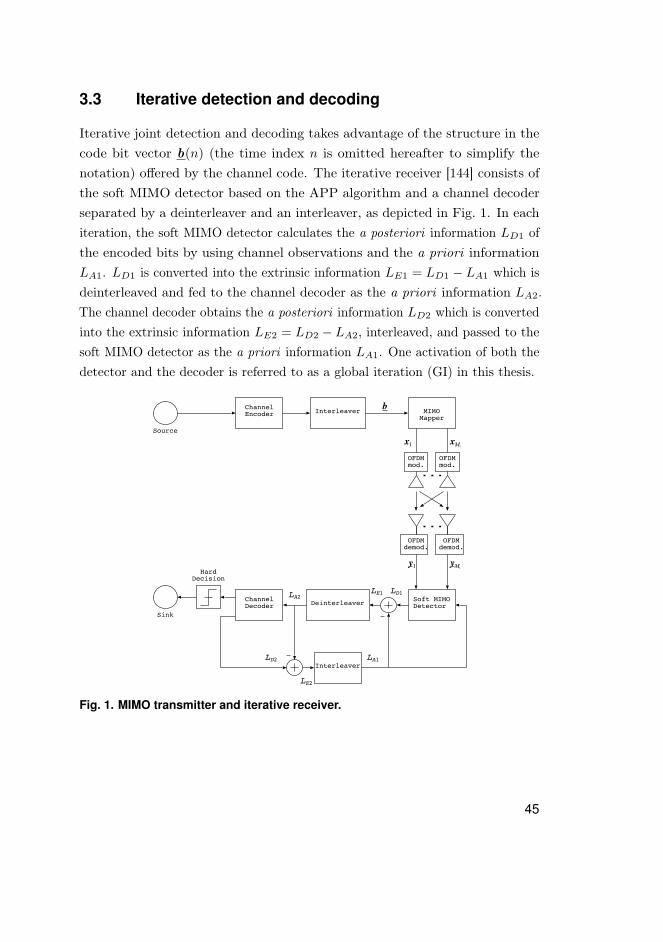
Iterative joint detection and decoding takes advantage of the structure in thecode bit vector b(n) (the time index n is omitted hereafter to simplify thenotation) offered by the channel code. The iterative receiver [144] consists ofthe soft MIMO detector based on the APP algorithm and a channel decoderseparated by a deinterleaver and an interleaver, as depicted in Fig. 1. In eachiteration, the soft MIMO detector calculates the a posteriori information LD1 ofthe encoded bits by using channel observations and the a priori informationLA1. LD1 is converted into the extrinsic information LE1 = LD1 − LA1 which isdeinterleaved and fed to the channel decoder as the a priori information LA2.The channel decoder obtains the a posteriori information LD2 which is convertedinto the extrinsic information LE2 = LD2 − LA2, interleaved, and passed to thesoft MIMO detector as the a priori information LA1. One activation of both thedetector and the decoder is referred to as a global iteration (GI) in this thesis.

MIMOMapper

InterleaverChannelEncoder

Source

Sink

HardDecision

Deinterleaver

Interleaver

ChannelDecoder

Soft MIMODetector

OFDMmod.

OFDMmod.

OFDMdemod.

OFDMdemod.

LD1LA2

LD2 LA1

LE1

LE2

b

x1 xMt

y1 yMt

Fig. 1. MIMO transmitter and iterative receiver.

45

The a posteriori information from the detector is defined as bit log-likelihoodratios (LLRs). The LLR of the qth encoded bit, q = 1, ...,McMt, can be writtenas

LD1(bq|y) = lnPr(bq = +1|y)

Pr(bq = −1|y). (3)

Using Bayes’ theorem and assuming the bits in x are statistically independent ofone another due to interleaving after channel coding, the soft output values aregiven by

LD1(bq|y) = LA1(bq) + ln

∑b∈Bq,+1

exp(Λ(b, b [q], lA1,[q]|y ,H ))∑b∈Bq,−1

exp(Λ(b, b [q], lA1,[q]|y ,H ))︸︷︷︸LE1(bq|y )

, (4)

whereΛ(b, b [q], lA1,[q]|y ,H ) = − 1

2σ2w‖y −Hx‖2 +

1

2bT

[q]lA1,[q], (5)

and Bq,±1 are the sets of 2MtMc possible bit vectors b with bq = ±1, i.e.,Bq,±1 = b|bq = ±1, b is the part of b corresponding to the desired subcarrier,b [q] denotes the subvector of b obtained by omitting its qth element bq, lA1,[q] isthe vector of all LA1 values corresponding to one subcarrier, also omitting bq,and x =M(b). In this thesis, (4) is also referred to as the a posteriori (APP)algorithm.

The complexity of computing LD1(bq|y) increases exponentially with Mc

and Mt, and, thus, it is computationally too intensive in many cases. However,the vast majority of the elements of B have insignificant contributions to theLLR-value. List detectors search a candidate list L with K << 2McMt bit vectorsby omitting those insignificant contributors, and, thus, approximate (4) as

LD1(bq|y) ≈ LD1(bq|y) = LA1(bq) + ln

∑b∈Lq,+1

exp(Λ(b, b [q], lA1,[q]|y ,H ))∑b∈Lq,−1

exp(Λ(b, b [q], lA1,[q]|y ,H ))︸︷︷︸LE1(bq|y )

,

(6)with lower complexity and minor degradation in performance.

46

4 Detection of spatially multiplexed signals inMIMO-OFDM

This chapter focuses on the MIMO detection part of the iterative receiver. Perfectchannel information is assumed to be available at the receiver. A new list detectornamed the list parallel interference cancellation (PIC) detector is derived in thischapter. The LMMSE MIMO detection algorithm is also presented because it isused in the initialization of the list PIC detector. The performance of the list PICdetector is studied with different modulation methods and antenna configurations.Its performance and the complexity are compared to the important list spheredetection algorithms. This chapter shows how the convergence of iterativedetection and decoding can be accelerated by re-calculating the candidate list inaddition to the LLR values in each global iteration. As a summary, the mainoriginal contributions of this chapter are the derivation of the list PIC algorithmand introducing list re-calculation in iterative detection and decoding.

The chapter is organized as follows. Section 4.1 presents the LMMSEalgorithm for MIMO detection. The list PIC detector is derived in Section 4.2.The method of list re-calculation in iterative detection and decoding is presented inSection 4.3. Section 4.4 provides performance as well as complexity comparisons.Finally, conclusions are drawn in Section 4.5.

4.1 Linear minimum mean square algorithm

Linear minimum mean square error detection minimizes the mean square error(MSE) between the transmitted symbols and the soft estimates of the transmittedsymbols as

GLMMSE = arg minGLMMSE

E(‖x −GH

LMMSEy‖2). (7)

After solving (7), the LMMSE filtering matrix is expressed by

GLMMSE = (H HH + σ2wI )−1H H (8)

and the resulting filter output, i.e., the soft decision of the transmitted symbolvector is

xLMMSE = (H HH + σ2wI )−1H Hy . (9)

47

The hard decisions xLMMSE are obtained simply by quantizing the soft decisionsto the closest constellation points.

4.2 List parallel interference cancellation algorithm

The list parallel interference cancellation (PIC) detector combines the tree searchmethodology of LSD receivers with the SAGE detector. In the SAGE detector[191], the received signal y is viewed as the “incomplete" data and the “complete"data zmt ∈CMr is defined as

zmt = hmtxmt + w , 1 ≤ mt ≤Mt. (10)

Thus, zmt can be seen as the component of the received signal transmittedfrom the mtth transmit antenna through the channel hmt and corrupted by thenoise, where hmt

is the mtth column of the frequency domain channel matrixH . Assuming known channel state information in the receiver, the “complete"data is estimated in the expectation (E) step as

zmt = hmt xmt + (y −Mt∑m′t=1

hm′t xm′t) = y −Mt∑

m′t=1

m′t 6=mt

hm′t xm′t , (11)

where xmt , mt = 1, ...,Mt are initial guesses or current estimates of xmt . Theinitial guess can be obtained for example by using the LMMSE detector. Onecan note that the estimation of the “complete" data is in practise done by PIC.In the maximization (M) step, the new estimate for the symbol xmt is calculatedas

xmt = arg minxmt∈Ω

||zmt − hmtxmt ||2. (12)

The E and M steps are iterated and the symbol estimate for each layer is updatedin turn. Finally, there is one estimate for the transmitted symbol vector. Using(11) in (12), one can easily see that (12) gives the Euclidean distance (ED) d(x )

for the symbol vector x ∈CMt in which all but the mtth element are from theprevious iterations.

The convergence properties of the SAGE algorithm are poor in detection[191]. The other defect of the SAGE algorithm as ML approximation is that asignificant performance loss may be caused in the channel coded systems if it

48

is used instead of the optimal APP detection prior to the soft input decoder.To solve the defects, we modify the algorithm in such a way that all |Ω| − 1

candidates are not necessarily dropped, but instead the K best candidatesare stored in every iteration. This modification enables the adoption of thetree search methodologies used in the LSD receivers into the new algorithm.The resulting SAGE based list detector produces a list of candidates for thetransmitted symbols starting from a single initial guess, and, thus, approximatesthe optimal APP detector. We call the resulting list detector the list PICdetector, since the estimation of the “complete" data can be seen as parallelinterference cancellation.

The algorithm can be illustrated with a tree structure as in Fig. 2, where abinary modulation is assumed to simplify the illustration. In the root layer,we have an initial guess of the transmitted symbol vector. Based on that, the“complete" data is calculated for the first layer (mt = 1) by using (11). Then,based on the “complete" data, the cost for all the possible symbol candidatescan be calculated by using (12). The K best candidates are stored and used asinitial guesses for the next layer. In the ith layer, in all the initial guesses, theelements xi+1, ..., xMt are inherited from the first initial guess. The “complete"data corresponding to each initial guess is calculated for the next layer. Then, inthe M step, the cost for each possible symbol candidate over all “complete" dataspaces is calculated and the K best candidates are stored. The algorithm goesthrough the tree so that there are K different paths left at all times. The searchscheme is a breadth-first algorithm [116] and the same as that used with theK-best LSD. The List PIC Algorithm is detailed in Algorithm 1.

Root layer

Layer n=1

Layer 2

Layer 3

Layer 4

Fig. 2. A tree structure with 4 transmit antennas and BPSK modulation.

49

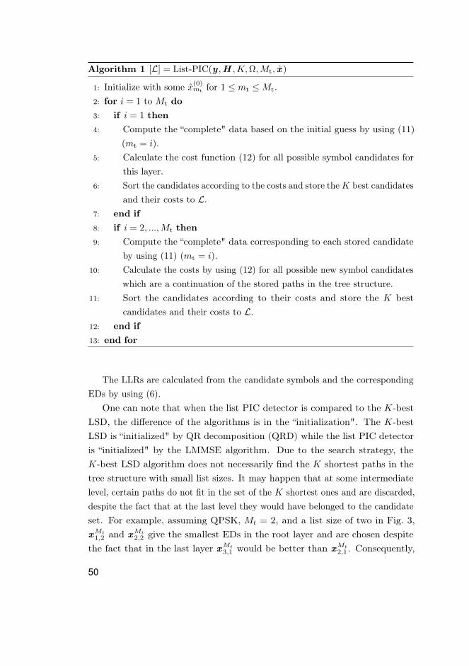
Algorithm 1 [L] = List-PIC(y ,H ,K,Ω,Mt, x )

1: Initialize with some x(0)mt for 1 ≤ mt ≤Mt.

2: for i = 1 to Mt do3: if i = 1 then4: Compute the “complete" data based on the initial guess by using (11)

(mt = i).5: Calculate the cost function (12) for all possible symbol candidates for

this layer.6: Sort the candidates according to the costs and store theK best candidates

and their costs to L.7: end if8: if i = 2, ...,Mt then9: Compute the “complete" data corresponding to each stored candidate

by using (11) (mt = i).10: Calculate the costs by using (12) for all possible new symbol candidates

which are a continuation of the stored paths in the tree structure.11: Sort the candidates according to their costs and store the K best

candidates and their costs to L.12: end if13: end for

The LLRs are calculated from the candidate symbols and the correspondingEDs by using (6).

One can note that when the list PIC detector is compared to the K-bestLSD, the difference of the algorithms is in the “initialization". The K-bestLSD is “initialized" by QR decomposition (QRD) while the list PIC detectoris “initialized" by the LMMSE algorithm. Due to the search strategy, theK-best LSD algorithm does not necessarily find the K shortest paths in thetree structure with small list sizes. It may happen that at some intermediatelevel, certain paths do not fit in the set of the K shortest ones and are discarded,despite the fact that at the last level they would have belonged to the candidateset. For example, assuming QPSK, Mt = 2, and a list size of two in Fig. 3,xMt

1,2 and xMt2,2 give the smallest EDs in the root layer and are chosen despite

the fact that in the last layer xMt3,1 would be better than xMt

2,1 . Consequently,

50

the problem is that the algorithm makes final decisions in every layer with noinformation from the forthcoming layers. As a solution, different search strategieshave been proposed, including depth-first [192] and metric-first [193] methods.From these strategies, especially the metric-first scheme is a promising approach.However, the advantage of the breadth-first search strategy is straightforwardimplementation, as discussed in [194].

x21,2 x2

2,2 x23,2 x2

4,2

x21,1 x2

2,1 x23,1

Fig. 3. An example of possible problem of breadth-first search with small list sizes.

In the case of the list PIC detector, information from the other layers isavailable when the decision on the paths to be discarded is made. The cancellingof the layers not in focus using the initial guess “distributes" the informationbetween the layers. Let us consider the same example as with the K-best LSDin Fig. 3. If the initialization for the second layer is close enough to the symbolrepresented by xMt

1,1 , xMt2,1 and xMt

3,1 , instead of choosing xMt1,2 and xMt

2,2 as wasthe case with the K-best LSD, xMt

1,2 and xMt3,2 will be chosen in the case of the

list PIC detector. Consequently, in the best case, the list PIC algorithm solvesthe convergence problems of the conventional SAGE detector and improves theperformance of the breadth-first search scheme with small list sizes. However,the potential frailty of the list PIC algorithm is its sensitivity to the initial guess.This sensitivity is common with the EM based methods and is well addressed inthe literature [151].

Analytical study of the list PIC algorithm is not carried out in this thesis.However, the approach taken in [195] to analyze symbol error probability ofthe fixed complexity sphere decoder (FSD) [196] in uncoded system might be

51

useful for the list PIC detector as well. When considering the error probability,the error event is separated into two mutually exclusive events depending onwhether the transmitted symbol vector x belongs to the candidate list. In [195]it is shown that Pr(x /∈ L) defines how much a SD loses to the ML detector.This is of course intuitively obvious. To define Pr(x /∈ L) one has to define theprobabilities for all the possible events in which the correct path is discarded inthe tree search. This is left for future work.

4.3 List re-calculation in iterative detection and decoding

The conventional way of using the a priori information from the decoder in thesoft MIMO detector is to re-calculate the LLRs. However, if the soft MIMOdetector is based on a list detector, the performance can potentially be improvedby re-calculating also the candidate list and using a priori information in the listre-calculation. This is natural, because using the decoder output as a prioriinformation, the quality of the candidate list is likely to be improved. In otherwords, the list detection uses the decoder output in addition to the conventionalEuclidean distance metric in the detection process. The cost of a candidate isexpressed as

Λ(b, lA1|y ,H ) = − 1

2σ2w‖y −Hx‖2 +

1

2bTlA1, (13)

when a priori information is used in the list re-calculation. Notice that now lA1

includes also the qth bit and

LD1(bq|y) = ln

∑b∈Lq,+1

exp(Λ(b, lA1|y ,H ))∑b∈Lq,−1

exp(Λ(b, lA1|y ,H )). (14)

The extrinsic information is formed by LE1(bq|y) ≈ LD1(bq|y)− LA1(bq). If thelist is re-calculated, also a new initial guess of the symbol vectors for the list

52

PIC detector can be calculated from the LLRs produced by the decoder as [141]

E(xmt) =∑

x′mt∈Ω

x′mtPr(xmt = x′mt

) (15)

= (1

2)Mc

∑x′mt∈Ω

x′mt

×Mc∏mc=1

(1 + bmctanh(LD2(bmc

)/2)),

where Mc is the number of bits per constellation point and Ω is the set ofconstellation points.

4.4 Numerical examples

Monte Carlo computer simulations were conducted to study the performance ofthe proposed algorithms. The two different ways of using a priori informationin the list detector were studied. The list PIC detector was compared tothe APP algorithm, the K-best LSD, and the IR-LSD when operating as asoft MIMO detector together with turbo coding at a rate of 1/2. The turbocoding scheme was a parallel concatenated convolutional code (PCCC) with two8-state encoders and an internal interleaver followed by puncturing, multiplexing,and bit-level interleaving. The constituent codes (CCs) are rate 1/2 binaryrecursive systematic convolutional codes [197]. The turbo decoder consists oftwo component log-maximum a posteriori (MAP) decoders [138], and 8 decoderiterations were performed. Coding was performed over the transmit antennasand one code word consisted of QPSK, 16QAM, or 64QAM symbols transmittedover one OFDM symbol.

A symbol duration of 66.7 µs and a cyclic prefix length of 16.68 µs wereassumed. The number of subcarriers was 512. The carrier frequency was 2.4GHz. A mobile speed of 50 km/h was studied. Two MIMO configurations,namely 2× 2 and 4× 4, were employed in the simulations. The simulations wereperformed with the typical urban channel model [198]. The key parameters ofthe stochastic MIMO radio channel model are summarized in Table 1 and itspower delay profile (PDP) in Table 2. The SNR is defined as ES/N0, where ES

is the symbol energy received by a receive antenna and N0I is the covariancematrix of the noise.

53

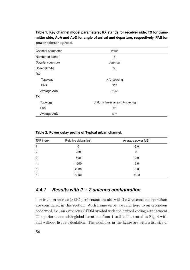
Table 1. Key channel model parameters; RX stands for receiver side, TX for trans-mitter side, AoA and AoD for angle of arrival and departure, respectively, PAS forpower azimuth spread.

Channel parameter Value

Number of paths 6

Doppler spectrum classical

Speed [km/h] 50

RX

Topology λ/2-spacing

PAS 35o

Average AoA 67, 5o

TX

Topology Uniform linear array 4λ-spacing

PAS 2o

Average AoD 50o

Table 2. Power delay profile of Typical urban channel.

TAP index Relative delays [ns] Average power [dB]

1 0 -3.0

2 200 0

3 500 -2.0

4 1600 -6.0

5 2300 -8.0

6 5000 -10.0

4.4.1 Results with 2 × 2 antenna configuration

The frame error rate (FER) performance results with 2×2 antenna configurationsare considered in this section. With frame error, we refer here to an erroneouscode word, i.e., an erroneous OFDM symbol with the defined coding arrangement.The performance with global iterations from 1 to 5 is illustrated in Fig. 4 withand without list re-calculation. The examples in the figure are with a list size of

54

two and for QPSK modulation. Ideal channel state information (CSI) is assumedat the receiver. One can note that global iterations after the fifth iterationprovide no substantial benefit in either case. Furthermore, if list re-calculation isused, three global iterations result in better performance than 5 global iterationswithout list re-calculation.

8 8.5 9 9.5 10 10.5 11 11.5 12 12.5 1310−2

10−1

100

ES/N0 [dB]

FER

2−List PIC 1 GI2−List PIC 2 GI2−List PIC 3 GI2−List PIC 4 GI2−List PIC 5 GI2−List PIC 2 GI list re−calc.2−List PIC 3 GI list re−calc.2−List PIC 4 GI list re−calc.2−List PIC 5 GI list re−calc.

Fig. 4. FER performance in typical urban channel with Global iterations 1 to 5(QPSK 2×2), ([1],published by permission of IEEE).

The FER performance of the detectors with ideal CSI at the receiver ispresented for QPSK, 16QAM, and 64QAM constellations in Figs. 5–7, respectively.From Fig. 5, one can note that with a list size of four, the list PIC algorithm losesinsignificantly to the APP algorithm when QPSK is considered as a modulationscheme. The K-best LSD and the IR-LSD offer exactly the same performance asthe list PIC detector with a list size of four (not shown in the figure). When alist size of two is used, the list detectors are outperformed by the APP algorithm.However, the performance degradation of the K-best LSD is more than thatof the list PIC detector, while the IR-LSD outperforms both of the other listdetectors.

55

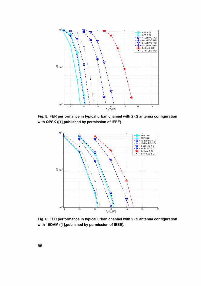
6 8 10 12 14 16 1810−2

10−1

100

ES/N0 [dB]

FER

APP 1 GIAPP 5 GI4−List PIC 1 GI4−List PIC 5 GI2−List PIC 1 GI2−List PIC 5 GI2−Kbest 5 GI2−IR−LSD 5 GI

Fig. 5. FER performance in typical urban channel with 2×2 antenna configurationwith QPSK ([1],published by permission of IEEE).

14 15 16 17 18 19 2010−2

10−1

100

ES/N0 [dB]

FER


Fig. 6. FER performance in typical urban channel with 2×2 antenna configurationwith 16QAM ([1],published by permission of IEEE).

56

21 21.5 22 22.5 23 23.5 24 24.5 25 25.5 2610−2

10−1

100

ES/N0 [dB]

FER

256−List PIC 1 GI256−List PIC 5 GI32−List PIC 1 GI32−List PIC 5 GI32−Kbest 5 GI16−List PIC 1 GI16−List PIC 5 GI16−Kbest 5 GI16−IR−LSD 5 GI


A list size of 16 reaches optimal performance with the list PIC detectorwhen 16QAM is used, as can be seen in Fig. 6. Again, the K-best LSD and theIR-LSD exhibit exactly the same performance as the list PIC detector with a listsize of 16 and have been excluded from the figure. The superiority of the listPIC detector over the K-best LSD can be seen with a list size of 8. However,the IR-LSD outperforms the list PIC detector, gaining about 0.5 dB.

The performance of the APP algorithm is not simulated for the 64QAM casedue to the time-consuming simulation length. Instead, the list PIC detector witha list size of 256 is used as a reference in Fig. 7. The performance of the list PICdetector deteriorates insignificantly when the list size is decreased to 32, whilethe performance loss of the K-best LSD is more noticeable. The superiorityof the list PIC detector over the K-best LSD is further emphasized by a listsize of 16 in this case. The IR-LSD offers practically the same performancewith a list size of 16 as the list PIC detector with a list size of 32. Within thepresented examples, at least 1 dB of gain is achieved by exchanging the extrinsicinformation between the detector and the decoder.

57

4.4.2 Results with 4 × 4 antenna configuration

The FER performance results of the turbo coded OFDM system in a typicalurban channel with a 4× 4 antenna configuration are considered in this section.The performance with global iterations from 1 to 5 is illustrated in Fig. 8 withand without list re-calculation, assuming QPSK modulation and a list size of8. One can note that the global iterations after the fifth iteration provide nosubstantial benefit, as was the case also with the 2× 2 antenna configuration. Iflist re-calculation is used, two global iterations result in the same performance asfive global iterations without list re-calculation.

9 9.5 10 10.5 11 11.5 12 12.5 1310−2

10−1

100

ES/N0 [dB]

FER

8−List PIC 1 GI8−List PIC 2 GI8−List PIC 3 GI8−List PIC 4 GI8−List PIC 5 GI8−List PIC 2 GI list re−calc.8−List PIC 3 GI list re−calc.8−List PIC 4 GI list re−calc.8−List PIC 5 GI list re−calc.

Fig. 8. FER performance in typical urban channel with Global iterations 1 to 5(QPSK 4×4) ([1],published by permission of IEEE).

The performances using QPSK and 16QAM with ideal CSI are presentedin Figs. 9 and 10, respectively. One can see that in the case of QPSK with alist size of 8, the list PIC detector offers some gain over the K-best LSD. TheIR-LSD with a list size of 8 offers better performance than the other two witha list size of 16. Then, in the case of 16QAM, the list PIC detector starts tolose to the K-best LSD. The reason for such behavior is that the initial guess

58

provided by the LMMSE detector is not accurate enough in the case of the 4× 4

antenna configuration with 16QAM and with correlated transmit and receiveantennas [101]. This is supported by the simulation result in which the knowntransmitted symbols are given as an initial guess to the list PIC detector witha list size of 256 and one global iteration is performed. One can see that thisresults in better performance than with the K-best LSD with the same list sizeand with 5 global iterations. The IR-LSD with a list size of 32 gives almostthe same performance as the K-best LSD with a list size of 64. The extrinsicinformation exchange gives about 1 dB of gain in the presented examples.

8 8.5 9 9.5 10 10.5 11 11.5 12 12.5 1310−2

10−1

100

Es/N0 [dB]

FER

APP 1 GIAPP 5 GI16−List PIC 1 GI16−List PIC 5 GI16−Kbest 5 GI8−List PIC 1 GI8−List PIC 5 GI8−Kbest 5 GI8−IR−LSD 5 GI


59

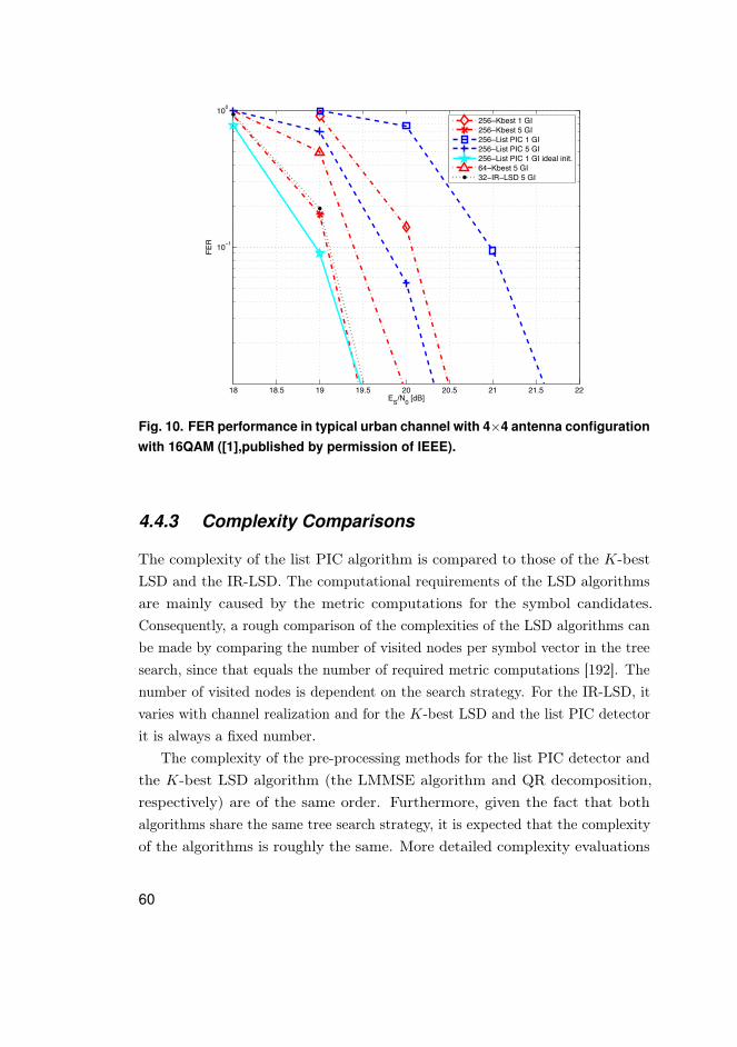
18 18.5 19 19.5 20 20.5 21 21.5 22

10−1

100

ES/N0 [dB]

FER

256−Kbest 1 GI256−Kbest 5 GI256−List PIC 1 GI256−List PIC 5 GI256−List PIC 1 GI ideal init.64−Kbest 5 GI32−IR−LSD 5 GI


4.4.3 Complexity Comparisons

The complexity of the list PIC algorithm is compared to those of the K-bestLSD and the IR-LSD. The computational requirements of the LSD algorithmsare mainly caused by the metric computations for the symbol candidates.Consequently, a rough comparison of the complexities of the LSD algorithms canbe made by comparing the number of visited nodes per symbol vector in the treesearch, since that equals the number of required metric computations [192]. Thenumber of visited nodes is dependent on the search strategy. For the IR-LSD, itvaries with channel realization and for the K-best LSD and the list PIC detectorit is always a fixed number.

The complexity of the pre-processing methods for the list PIC detector andthe K-best LSD algorithm (the LMMSE algorithm and QR decomposition,respectively) are of the same order. Furthermore, given the fact that bothalgorithms share the same tree search strategy, it is expected that the complexityof the algorithms is roughly the same. More detailed complexity evaluations

60

based on architecture design for the K-best LSD can be found from [147] and[199]. The detailed architecture design for the list PIC detector is subject tofurther research.

Simulated histograms of the number of visited nodes per symbol vector forthe list PIC detector, IR-LSD and K-best LSD algorithms using a list size of8 with 16QAM and a list size of 16 with 64QAM are shown in Fig. 11. Twotransmit antennas are assumed. One can note that the IR-LSD algorithm islikely to visit less nodes compared to the list PIC detector and the K-best LSDalgorithms. Consequently, the IR-LSD is the least complex in these cases. Thehardware resources have to be reserved according to the worst-case scenario.Thus, in the 16QAM case, the difference is not that big. The list PIC detectorand the K-best LSD use the same search strategy. Consequently, with the samelist sizes, the number of visited nodes is the same, meaning that their complexityis the same as well.

0 50 100 150 200 2500

0.5

1

1.5

2

2.5

3

3.5x 105

# of visited nodes per symbol vector

# of

cas

es

(a)

0 200 400 600 800 1000 1200 1400 1600 18000

2

4

6

8x 104


# of

cas

es

(b)

8−IR ideal CSI, SNR 16dB 8−IR est. CSI, SNR 18 dB8−List PIC & 8−Kbest

16−IR ideal CSI, SNR 22 dB16−IR est. CSI, SNR 27 dB16−List PIC & 16−Kbest

Fig. 11. Histogram of the number of visited nodes per symbol vector for (a) 16-QAM and (b) 64-QAM with a 2×2 antenna configuration ([1],published by permis-sion of IEEE).

61

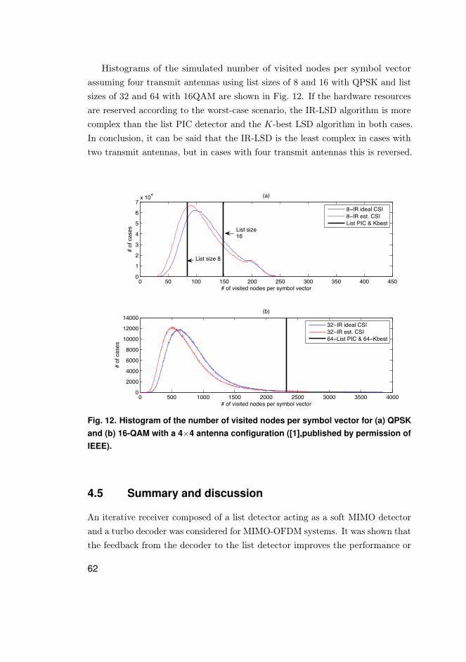
Histograms of the simulated number of visited nodes per symbol vectorassuming four transmit antennas using list sizes of 8 and 16 with QPSK and listsizes of 32 and 64 with 16QAM are shown in Fig. 12. If the hardware resourcesare reserved according to the worst-case scenario, the IR-LSD algorithm is morecomplex than the list PIC detector and the K-best LSD algorithm in both cases.In conclusion, it can be said that the IR-LSD is the least complex in cases withtwo transmit antennas, but in cases with four transmit antennas this is reversed.

0 500 1000 1500 2000 2500 3000 3500 40000

2000

4000

6000

8000

10000

12000

14000


# of

cas

es

(b)

0 50 100 150 200 250 300 350 400 4500

1

2

3

4

5

6

7x 104


# of

cas

es

(a)

8−IR ideal CSI8−IR est. CSIList PIC & Kbest

32−IR ideal CSI32−IR est. CSI64−List PIC & 64−Kbest

List size 8

List size16

Fig. 12. Histogram of the number of visited nodes per symbol vector for (a) QPSKand (b) 16-QAM with a 4×4 antenna configuration ([1],published by permission ofIEEE).

4.5 Summary and discussion

An iterative receiver composed of a list detector acting as a soft MIMO detectorand a turbo decoder was considered for MIMO-OFDM systems. It was shown thatthe feedback from the decoder to the list detector improves the performance or

62

enables the use of smaller list size values without compromising the performance.A method called list re-calculation was proposed to give further gain by using apriori information from the decoder to re-calculate the candidate list duringglobal iterations instead of only re-calculating the LLRs as is done conventionally.An open question is whether the cheapest way in terms of the complexity ofachieving a certain performance target is to utilize conventional global iterations,global iterations with list re-calculations, or a greater list size.

A novel list PIC detector was presented and compared to the optimal APPalgorithm, the K-best LSD, and the IR-LSD. The results showed that thelist PIC detector offers close to optimal performance with reduced complexityand a performance gain over the K-best LSD with proper initialization. Theinitialization plays an important role since the list PIC algorithm is based onthe SAGE algorithm and the SAGE algorithm is known to be sensitive to theinitial guess of the estimated parameters. The LMMSE proved out to be goodenough in the initialization for a 2× 2 antenna configuration. However, for a4× 4 antenna configuration with higher order modulations it was inadequate.The initialization might be improved by various techniques (such as latticereduction [107] or semidefinite relaxation based detection [128]), which could bea fruitful research topic. The IR-LSD offers performance gain over the otherstudied list detectors. However, in the case of a 2× 2 antenna configuration, thegain over the list PIC detector is not substantial. The complexity of the list PICdetector is of the same order as that of the K-best LSD, and the metric-firstbased IR search algorithm was found to be the less complex than the list PICdetector in a 2× 2 antenna configuration. However, taking into account that2× 2 antenna configuration and LMMSE detection will most likely be the firststep when employing MIMO processing; the list PIC detector might offer quitean attractive second step due to its straightforward implementation.

63

5 Channel estimation for MIMO-OFDM system

This chapter considers channel estimation for a MIMO-OFDM system. Thestructure of the iterative receiver with a channel estimator is presented. TheLS channel estimation algorithm is reviewed and its intensive computationalrequirements in DD mode are pointed out. The frequency domain (FD) SAGEDD channel estimation algorithm is discussed as a solution to reduce thecomputational complexity in the case of constant envelope constellations. Thetime domain (TD) SAGE channel estimation algorithm is derived to solve thecomplexity issue also with higher order constellations. MMSE channel estimationis reviewed. The implementation aspects of the LS, FD-SAGE, and MMSEchannel estimators are considered by presenting possible architecture designs forthem. The performance of the channel estimation algorithms is studied in variousscenarios. The main original contributions of this chapter are pointing out theproblem of the FD-SAGE algorithm with non-constant envelope constellations,the derivation of the TD-SAGE algorithm, architecture designs proposed forthe LS and FD-SAGE algorithms, and the MMSE filter approximation withpre-calculated filters.

The rest of the chapter is organized as follows. The structure of the iterativereceiver is presented in Section 5.1. Section 5.2 presents the LS channel estimationfor a MIMO-OFDM system. The FD-SAGE channel estimation algorithm isdetailed in Section 5.3. The TD-SAGE channel estimation algorithm is derivedin Section 5.4 followed by the presentation of MMSE filtering in Section 5.5. Theimplementation aspects of the channel estimation algorithms are discussed inSection 5.7. After presenting the simulation studies in Section 5.8, the conclusionsare drawn in Section 5.9.

5.1 Iterative receiver with channel estimator

The receiver structure with a channel estimator is shown in Fig. 13. The feedbackfrom the decoder to the channel estimator is required only when DD or iterativechannel estimation is applied. At the core of the receiver, iterative detection anddecoding are performed by the soft MIMO detector and the turbo decoder as

65

explained in Section 3.3. The iterations between the detector and the decoderare referred to as global iterations (GI). Symbol estimates are calculated asgiven in (15).

OFDM demod.

OFDM demod.

SoftMIMO

detector

Turbodecoder

Channelestimator

Interleaver

DeInterleaver

Decisions

LD1

LA1

LE1

LA2

LD2LE2

Symbolestimates

Fig. 13. Receiver structure with channel estimation.

Let us assume that one block includes multiple OFDM symbols and thechannel coding is over one OFDM symbol. In each block, the preamble symbolindex set is SP = 1, Nsymb/2+1, where Nsymb is the number of OFDM symbolsin the block. The cardinality of SP is denoted by NP. In preamble based LSestimation, the estimate given by the first preamble is used in the detection of thesymbols with indices 2...Nsymb/2 and the estimate given by the second preambleis used in the detection of the symbols with indices Nsymb/2 + 2...Nsymb. Inpreamble based LS estimation with MMSE post-processing, the two LS estimatesgiven by the preambles are filtered and as the output a channel estimate foreach OFDM symbol is given. In DD SAGE channel estimation, the LS estimateis used as an initial guess at the beginning of the frame, and after the secondOFDM symbol, the previous estimate is used to initialize the SAGE algorithms.The channel is re-estimated after the global iterations in DD estimation. Thechannel can be also re-estimated between the global iterations, which is referredto as iterative channel estimation in this thesis. It is also possible to initializethe SAGE algorithms by predicting the channel state by filtering the previouschannel estimates with the MMSE filter.

Let us consider coding over the whole block. The LS estimation with MMSEpost-processing is performed as explained above in the case of coding over oneOFDM symbol. However, DD SAGE estimation is now applied within the globaliterations. The initial channel estimate for the whole frame is given by LS

66

estimation with MMSE post processing, and after a certain number of globaliterations, the channel is re-estimated by the SAGE algorithm which is followedby a certain number of global iterations.

5.2 Least squares algorithm

The LS method is the best linear unbiased channel estimator in Gaussian noise[83]. The LS channel estimate for (1) is expressed as

hmr(n) =

(FHXH(n)X (n)F︸︷︷︸

CHC

)−1

FHXH(n)ymr

(n). (16)

Ignoring the leakage due to nonuniform channel tap spacing and assuming thatthe noise is white and Gaussian, the LS estimator is also the ML estimatorand optimal in the sense that it attains the Cramer-Rao lower bound (CRLB).One should also note that F in (16) is constructed from the truncated DFTmatrices resulting in zeroing the noise only components after the last channeltap in the time domain channel estimates. When transformed back to thefrequency domain, the accuracy of the estimates is improved due to the noisereduction. This belongs to the group of techniques referred to as transformdomain processing in the literature review part of the thesis.

The computation of the LS estimate requires an MtL×MtL matrix inversionwhich is a computationally intensive task. It was shown in [77] that with anorthogonal preamble sequence design, the matrix inversion can be avoidedwhile the estimator still achieves the minimum mean square error (MSE). Theorthogonal preamble sequence design reduces the matrix (CHC) to a diagonalmatrix PIMtL and, thus, (16) can be rewritten as

hmr(n) =

1

PFHXH(n)y

mr(n). (17)

However, if high spectral efficiency is sought and the LS method is used in DDmode, the inversion of a MTL×MTL matrix is inevitable.

67

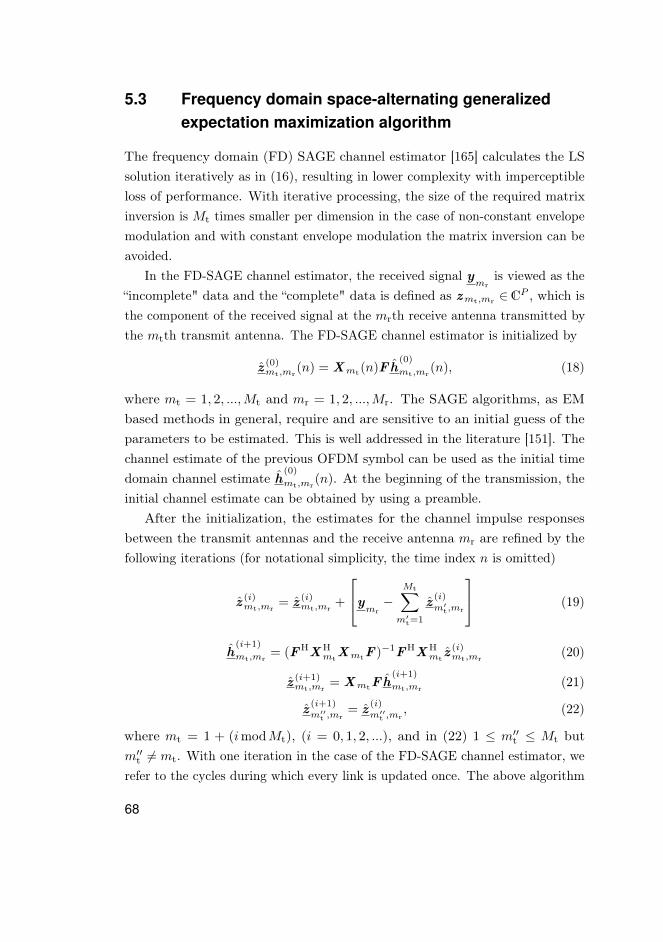
5.3 Frequency domain space-alternating generalizedexpectation maximization algorithm

The frequency domain (FD) SAGE channel estimator [165] calculates the LSsolution iteratively as in (16), resulting in lower complexity with imperceptibleloss of performance. With iterative processing, the size of the required matrixinversion is Mt times smaller per dimension in the case of non-constant envelopemodulation and with constant envelope modulation the matrix inversion can beavoided.

In the FD-SAGE channel estimator, the received signal ymr

is viewed as the“incomplete" data and the “complete" data is defined as zmt,mr ∈CP , which isthe component of the received signal at the mrth receive antenna transmitted bythe mtth transmit antenna. The FD-SAGE channel estimator is initialized by

z (0)mt,mr

(n) = Xmt(n)Fh(0)

mt,mr(n), (18)

where mt = 1, 2, ...,Mt and mr = 1, 2, ...,Mr. The SAGE algorithms, as EMbased methods in general, require and are sensitive to an initial guess of theparameters to be estimated. This is well addressed in the literature [151]. Thechannel estimate of the previous OFDM symbol can be used as the initial timedomain channel estimate h

(0)

mt,mr(n). At the beginning of the transmission, the

initial channel estimate can be obtained by using a preamble.After the initialization, the estimates for the channel impulse responses

between the transmit antennas and the receive antenna mr are refined by thefollowing iterations (for notational simplicity, the time index n is omitted)

z (i)mt,mr

= z (i)mt,mr

+

ymr−

Mt∑m′t=1

z (i)m′t,mr

(19)

h(i+1)

mt,mr= (FHXH

mtXmtF )−1FHXH

mtz (i)mt,mr

(20)

z (i+1)mt,mr

= XmtFh(i+1)

mt,mr(21)

z (i+1)m′′t ,mr

= z (i)m′′t ,mr

, (22)

where mt = 1 + (imodMt), (i = 0, 1, 2, ...), and in (22) 1 ≤ m′′t ≤ Mt butm′′t 6= mt. With one iteration in the case of the FD-SAGE channel estimator, werefer to the cycles during which every link is updated once. The above algorithm

68

transforms the LS channel estimation problem of a system with multiple transmitantennas as in (16) back to the multiple separate single transmit antenna LSchannel estimation problems performed serially. Consequently, the matrixinversion needed is Mt times smaller per dimension than the one required withDD-LS estimation. Furthermore, with constant envelope modulation, (20) canbe simplified to

h(i+1)

mt,mr= FHX−1

mtz (i)mt,mr

(23)

leading to the trivial inversion of the diagonal matrix Xmt . A more detaileddescription of the algorithm can be found in [165], in which constant envelopeconstellation is assumed and the drawback of the required inversion of a L× Lmatrix with non-constant envelope constellations was not treated.

5.4 Time domain space-alternating generalizedexpectation maximization algorithm

The time domain (TD) SAGE algorithm avoids the matrix inversion in theFD-SAGE algorithm with non-constant envelope modulations by choosing the“incomplete" and “complete" data spaces so that in the maximization step onlyone tap of one link is refined at a time. Then, the “incomplete" data is viewed asthe time domain received signal ymr

and the “complete" data omt,mr,l ∈CP ,which is the component of the time domain received signal at the mrth receiveantenna transmitted by the mtth transmit antenna and propagated through thelth path, is defined by

omt,mr,l = xmt,lhmt,mr,l+ wmr , (24)

where mt = 1, 2, ...,Mt, mr = 1, 2, ...,Mr, l = 0, ..., L − 1, the column vectorxmt,l = xmt(LCP + 1 − l : P + LCP − l), xmt = TCPFH

f diag(Xmt) is thetime domain signal from the mtth transmit antenna including the CP, TCP =

[ITLCP

ITP ]T, ILCP contains the last LCP rows from I P , LCP is the length of

the cyclic prefix, diag(·) takes the diagonal of a matrix and makes it a vector,and wmr is the noise term of (1) in the time domain. The time domain SAGEestimator is initialized by

o(0)mt,mr,l

= xmt,lh(0)

mt,mr,l, (25)

69

where mt = 1, 2, ...,Mt, mr = 1, 2, ...,Mr, and l = 0, ..., L − 1. The channelestimate of the previous OFDM symbol is used as the initial channel estimatesimilarly as with the FD-SAGE channel estimator. After the initialization, theestimates of the channel impulse responses between the transmit antennas andthe receive antenna mr are refined tap by tap through the following iterations

o(i)mt,mr,l

= o(i)mt,mr,l

+

ymr−

Mt∑m′t=1

L−1∑l′=0

o(i)m′t,mr,l′

(26)

h(i+1)

mt,mr,l(n) =xHmt,lo

(i)mt,mr

(n)

xHmt,lxmt,l

(27)

o(i+1)mt,mr,l

(n) = xmt,lh(i+1)

mt,mr,l(28)

o(i+1)m′′t ,mr,l′′

(n) = o(i)m′′t ,mr,l′′

, (29)

where mt = 1 + (imod (Mt + L)), l = (imodL), (i = 0, 1, 2, ...), and in (29)1 ≤ m′′t ≤Mt but m′′t 6= mt as well as 0 ≤ l′′ ≤ L but l′′ 6= l. With one iterationin the case of the TD-SAGE estimator, we refer to the cycles during which everylink is updated once.

5.5 Minimum mean square error algorithm

The LS and SAGE algorithms do not exploit the time domain correlation of thechannel in the estimation. The noise is totally neglected by them as well. Thus,the estimation performance can be further improved by post-processing the LSand SAGE channel estimates with a filter based on the MMSE criterion [91]. Ittakes advantage of the temporal correlation of the channel impulse response(CIR) taps between consecutive OFDM symbols as well as taking the noise levelinto account. The autocorrelation of the CIR taps can be expressed as

Σhmt,mr,l(n),hmt,mr,l(n′) = ρmt,mr(n− n′)σ2

hmt,mr,l, (30)

where ρmt,mr(n− n′) denotes the temporal correlation between the channel tapsat time instances n and n′, and σ2

hmt,mr,l= E(h∗mt,mr,l

hmt,mr,l). The temporalcorrelation depends on the Doppler spectrum and it is distributed according toJakes’ model. Thus, the temporal correlation can be written as

ρmt,mr(n− n′) = J0

(2πfd(n′ − n)TB

), (31)

70

where J0(·) denotes the zeroth-order Bessel function of the first kind, fd is theDoppler frequency, and TB is the duration of an OFDM symbol. In order toobtain the MMSE estimates, we define an LS channel estimate vector as

h<LS>mt,mr,l =

[h<LS>mt,mr,l

(n1) . . . h<LS>mt,mr,l

(nNP)]T∈ CNP , n ∈ SP . (32)

The MMSE CIR estimate for the link between the mtth transmit antenna andthe mrth receive antenna at time n can now be expressed as

h<MMSE>mt,mr,l

(n) = vmt,mr,l(n)h<LS>mt,mr,l ∈C, (33)

where the Wiener filtering vector vmt,mr,l(n) is defined as

vmt,mr,l(n) = Σhmt,mr,l(n),h

<LS>mt,mr,l

Σ−1

h<LS>mt,mr,l

. (34)

The cross-covariance vector Σhmt,mr,l(n),h

<LS>mt,mr,l

∈CNP and the autocovariance

matrix Σh

<LS>mt,mr,l

∈ CNP×NP in (34) are defined as

Σhmt,mr,l(n),h

<LS>mt,mr,l

=[ρ(n− n1) . . . ρ(n− nNP)

]σ2hmt,mr,l

(35)

Σh

<LS>mt,mr,l

=

ρ(n1 − n1) . . . ρ(n1 − nNP)

.... . .

...ρ(nNP − n1) . . . ρ(nNP − nNP)

σ2hmr,mt,l

+ Σw, (36)

where the noise covariance matrix is Σw = σ2w [CHC]u,sINP , u = (mt − 1)Mt + l,and s = (mt − 1)Mt + l.

5.6 Complexity comparison between LS, SAGE, andMMSE channel estimators

The complexity of the TD-SAGE channel estimator is compared to those of theFD-SAGE channel estimator, the LS algorithm in DD and preamble based modeand MMSE filtering. For the FD-SAGE channel estimator, the complexity ispresented in both simplified form for constant envelope constellation and ingeneral form for non-constant envelope constellations. The required number ofcomplex multiplications and divisions for the algorithms is presented in symbolicform in Tables 3 and 4, respectively. In Table 5, an example of the number of

71

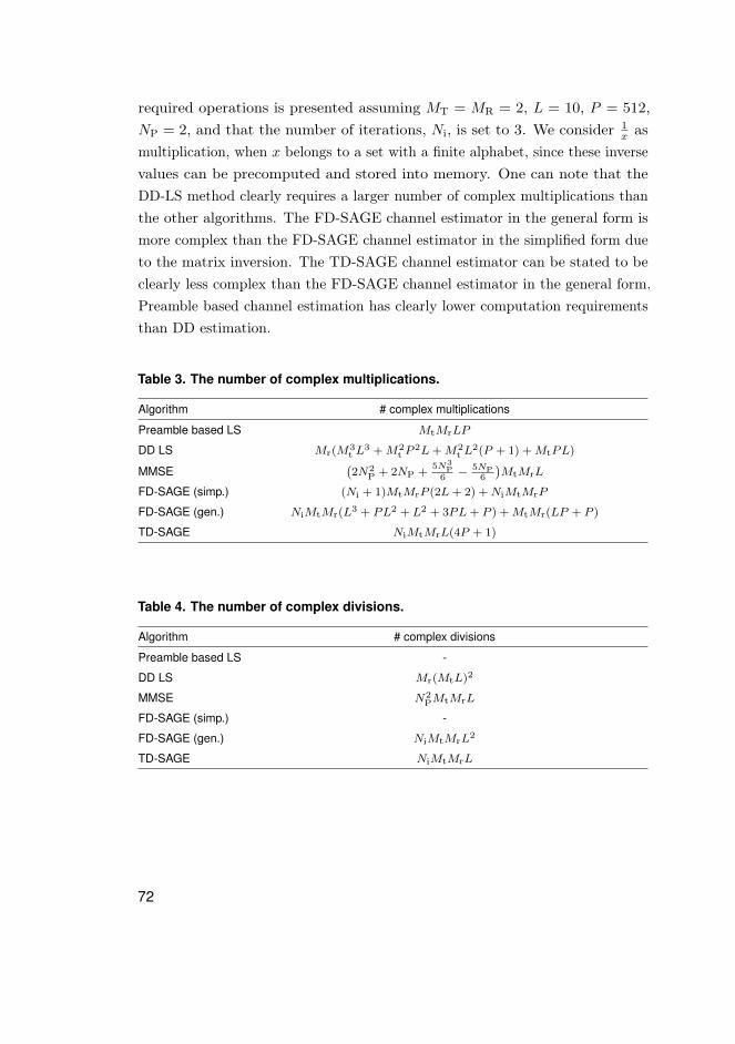
required operations is presented assuming MT = MR = 2, L = 10, P = 512,NP = 2, and that the number of iterations, Ni, is set to 3. We consider 1

x asmultiplication, when x belongs to a set with a finite alphabet, since these inversevalues can be precomputed and stored into memory. One can note that theDD-LS method clearly requires a larger number of complex multiplications thanthe other algorithms. The FD-SAGE channel estimator in the general form ismore complex than the FD-SAGE channel estimator in the simplified form dueto the matrix inversion. The TD-SAGE channel estimator can be stated to beclearly less complex than the FD-SAGE channel estimator in the general form.Preamble based channel estimation has clearly lower computation requirementsthan DD estimation.

Table 3. The number of complex multiplications.

Algorithm # complex multiplications

Preamble based LS MtMrLP

DD LS Mr(M3t L

3 +M2t P

2L+M2t L

2(P + 1) +MtPL)

MMSE(2N2

P + 2NP +5N3

P6

− 5NP6

)MtMrL

FD-SAGE (simp.) (Ni + 1)MtMrP (2L+ 2) +NiMtMrP

FD-SAGE (gen.) NiMtMr(L3 + PL2 + L2 + 3PL+ P ) +MtMr(LP + P )

TD-SAGE NiMtMrL(4P + 1)

Table 4. The number of complex divisions.

Algorithm # complex divisions

Preamble based LS -

DD LS Mr(MtL)2

MMSE N2PMtMrL

FD-SAGE (simp.) -

FD-SAGE (gen.) NiMtMrL2

TD-SAGE NiMtMrL

72

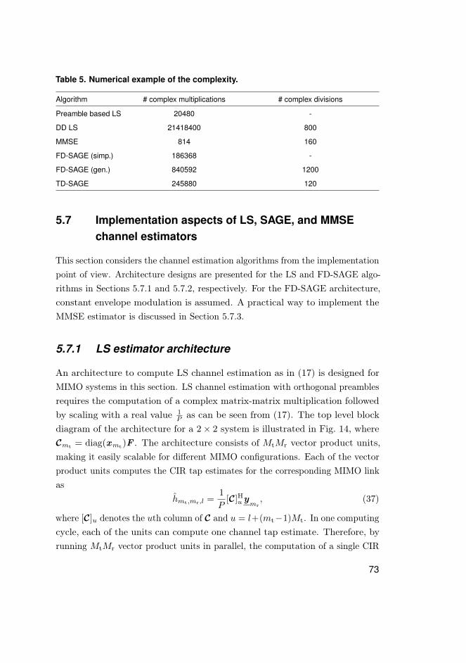
Table 5. Numerical example of the complexity.

Algorithm # complex multiplications # complex divisions

Preamble based LS 20480 -

DD LS 21418400 800

MMSE 814 160

FD-SAGE (simp.) 186368 -

FD-SAGE (gen.) 840592 1200

TD-SAGE 245880 120

5.7 Implementation aspects of LS, SAGE, and MMSEchannel estimators

This section considers the channel estimation algorithms from the implementationpoint of view. Architecture designs are presented for the LS and FD-SAGE algo-rithms in Sections 5.7.1 and 5.7.2, respectively. For the FD-SAGE architecture,constant envelope modulation is assumed. A practical way to implement theMMSE estimator is discussed in Section 5.7.3.

5.7.1 LS estimator architecture

An architecture to compute LS channel estimation as in (17) is designed forMIMO systems in this section. LS channel estimation with orthogonal preamblesrequires the computation of a complex matrix-matrix multiplication followedby scaling with a real value 1

P as can be seen from (17). The top level blockdiagram of the architecture for a 2× 2 system is illustrated in Fig. 14, whereCmt = diag(xmt)F . The architecture consists of MtMr vector product units,making it easily scalable for different MIMO configurations. Each of the vectorproduct units computes the CIR tap estimates for the corresponding MIMO linkas

hmt,mr,l =1

P[C]Huymr

, (37)

where [C]u denotes the uth column of C and u = l+(mt−1)Mt. In one computingcycle, each of the units can compute one channel tap estimate. Therefore, byrunning MtMr vector product units in parallel, the computation of a single CIR

73

vector hmt,mr takes L computing cycles in total. By further parallelization, onlyone computing cycle would be required with MtMrL vector product units.

h11 h12

h21 h22

aHb aHb

aHb aHb

C1y1

C2y1

C1y2

C2y2

Fig. 14. Top level structure of the LS estimator for a 2×2 MIMO system([9],published by permission of EURASIP).

The vector product unit is shown in more detail in Fig. 15. The unit takesfour scalar inputs and gives two scalar outputs. The elements of the input vectorsare read from inputs 1− 4, where 1 and 2 are for the real and imaginary parts of[C]u and 3 and 4 are for the real and imaginary parts of y

mr, respectively. The

vector product is computed by multiplying the elements of the two complexinput vectors and then adding the product to the sum of the previous elements’products. After all P products are summed, the final sum is multiplied by thescaling factor 1

P . The final result, i.e., the real and imaginary parts of hmt,mr,l

can then be read from outputs 5 and 6, respectively. The complex multiplicationof the vector elements is performed with three real multipliers to simplify theimplementation. For two complex numbers z1 = a+ bi and z2 = c+ di, wherea, b, c, d ∈ R and i =

√−1, the product z∗1z2 can be expressed in terms of the real

and imaginary parts as Rez∗1z2 = ac+ bd and Imz∗1z2 = ad− bc, requiringfour real multiplications. The same result can be calculated with only three realmultiplications by rearranging the equations as

Rez∗1z2 = (a+ b)(c+ d)− ad− bc

Imz∗1z2 = ad− bc. (38)

74

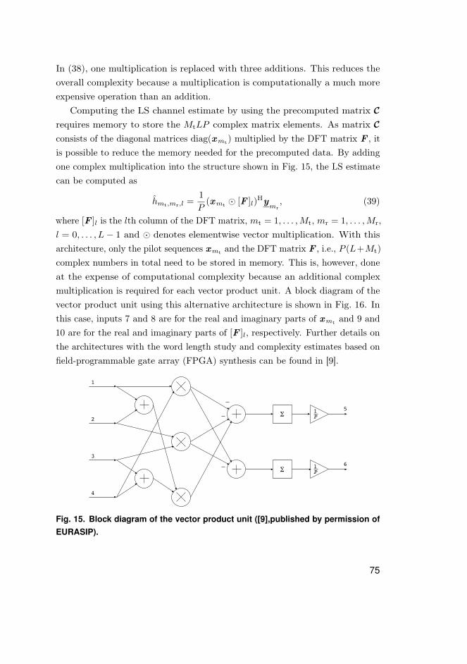
In (38), one multiplication is replaced with three additions. This reduces theoverall complexity because a multiplication is computationally a much moreexpensive operation than an addition.

Computing the LS channel estimate by using the precomputed matrix Crequires memory to store the MtLP complex matrix elements. As matrix Cconsists of the diagonal matrices diag(xmt) multiplied by the DFT matrix F , itis possible to reduce the memory needed for the precomputed data. By addingone complex multiplication into the structure shown in Fig. 15, the LS estimatecan be computed as

hmt,mr,l =1

P(xmt [F ]l)

Hymr, (39)

where [F ]l is the lth column of the DFT matrix, mt = 1, . . . ,Mt, mr = 1, . . . ,Mr,l = 0, . . . , L− 1 and denotes elementwise vector multiplication. With thisarchitecture, only the pilot sequences xmt and the DFT matrix F , i.e., P (L+Mt)

complex numbers in total need to be stored in memory. This is, however, doneat the expense of computational complexity because an additional complexmultiplication is required for each vector product unit. A block diagram of thevector product unit using this alternative architecture is shown in Fig. 16. Inthis case, inputs 7 and 8 are for the real and imaginary parts of xmt and 9 and10 are for the real and imaginary parts of [F ]l, respectively. Further details onthe architectures with the word length study and complexity estimates based onfield-programmable gate array (FPGA) synthesis can be found in [9].

1

2

4

3

1P

1P

!

!

5

6

Fig. 15. Block diagram of the vector product unit ([9],published by permission ofEURASIP).

75

1

2

4

3

1P

1P

!

!

5

6

7

8

9

10

Fig. 16. Block diagram of the alternative vector product unit ([9],published bypermission of EURASIP).

5.7.2 SAGE estimator architecture

An architecture design for the simplified FD-SAGE channel estimator for constantenvelope constellations is presented in this section. The top level architecture isillustrated in Fig 17. Only one receive antenna is assumed, but the design canbe easily generalized for multiple receive antennas by using similar architecturesin parallel. The architecture is divided into three main calculation blockscorresponding to (19), (21), and (23). The inputs of the estimator are y

mr, Xmt ,

h(0)

mt,mr, and mt = 1...Mt whereas the output is hmr

.

76

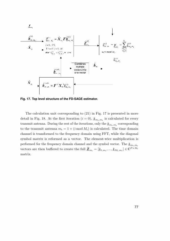
Fig. 17. Top level structure of the FD-SAGE estimator.

The calculation unit corresponding to (21) in Fig. 17 is presented in moredetail in Fig. 18. At the first iteration (i = 0), zmt,mr

is calculated for everytransmit antenna. During the rest of the iterations, only the zmt,mr

correspondingto the transmit antenna mt = 1 + (imodMt) is calculated. The time domainchannel is transformed to the frequency domain using FFT, while the diagonalsymbol matrix is reformed as a vector. The element-wice multiplication isperformed for the frequency domain channel and the symbol vector. The zmt,mr

vectors are then buffered to create the full Zmr= [z 1,mr

, ..., zMt,mr] ∈CP×Mt

matrix.

77

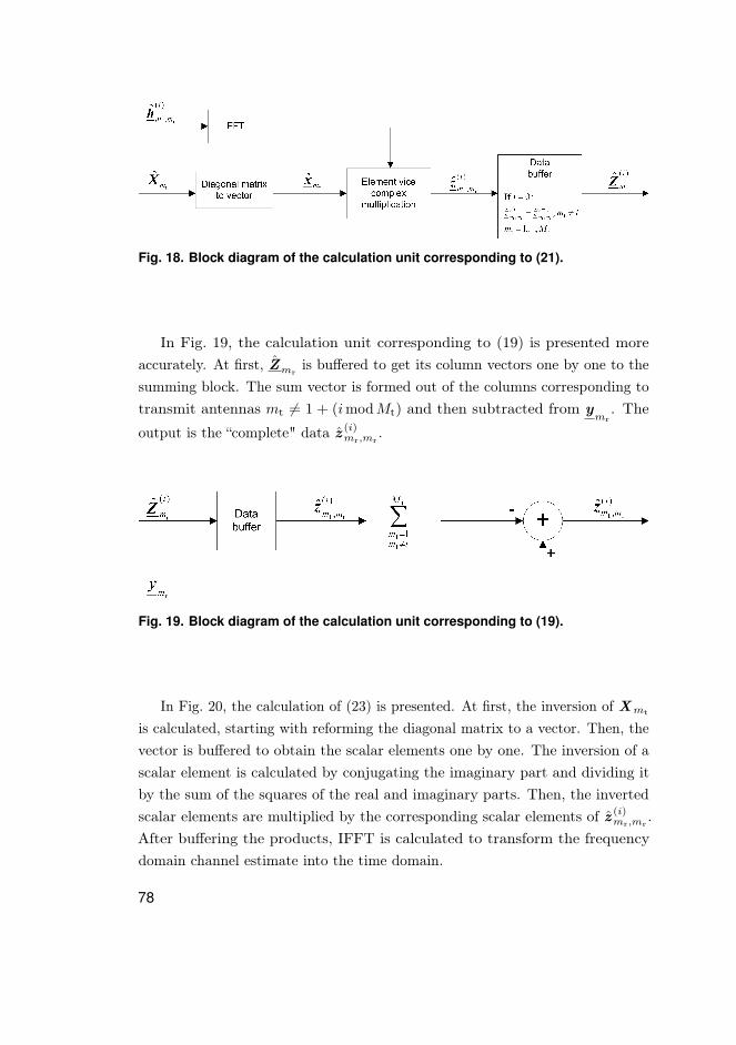
Fig. 18. Block diagram of the calculation unit corresponding to (21).

In Fig. 19, the calculation unit corresponding to (19) is presented moreaccurately. At first, Zmr

is buffered to get its column vectors one by one to thesumming block. The sum vector is formed out of the columns corresponding totransmit antennas mt 6= 1 + (imodMt) and then subtracted from y

mr. The

output is the “complete" data z (i)mr,mr

.


In Fig. 20, the calculation of (23) is presented. At first, the inversion of Xmt

is calculated, starting with reforming the diagonal matrix to a vector. Then, thevector is buffered to obtain the scalar elements one by one. The inversion of ascalar element is calculated by conjugating the imaginary part and dividing itby the sum of the squares of the real and imaginary parts. Then, the invertedscalar elements are multiplied by the corresponding scalar elements of z (i)

mr,mr.

After buffering the products, IFFT is calculated to transform the frequencydomain channel estimate into the time domain.

78


5.7.3 MMSE filter implementation

The MMSE estimator requires computation of an inversion of the covariancematrixΣ

h<LS>mt,mr,l

for each estimated channel tap. The dimensions of the covariancematrix depend on the size of the filtering window. One should note, however,that Σ

h<LS>mt,mr,l

is a Toeplitz matrix for which there exist fast and numerically

accurate inversion algorithms, such as the Levison algorithm [200] and thegeneralized Schur algorithm [201]. In this thesis, a simpler implementationapproach with a minor performance trade-off is followed.

From (34), it can be seen that the filtering vector only depends on theDoppler frequency and the noise variance. Consequently, for each mobile velocityand SNR value, a new filter vector must be computed. One way to approximateMMSE filtering is to pre-calculate the filters for some mobile velocities and SNRvalues beforehand. The filter closest to the prevailing circumstances is then used.With this approach, MMSE filtering will then only require the multiplication ofthe LS estimate vector with the filtering vector. This, naturally, only producesan approximation of the MMSE estimate when the actual velocity and SNRdiffer from the values used for computing the filtering vectors.

In Fig. 21, the analytical mean square error (AMSE) [91] performance of LSestimation with time domain MMSE filtering is shown in a typical urban channeland with a 2× 2 MIMO system. The dashed lines are with fixed pre-calculated

79

filters. Two pre-calculated filters are stored and the one closer to the prevailingconditions is used. One filter assumes a mobile speed of 55 km/h and a SNRvalue of 8.5 dB, and the other 85 km/h and a SNR value of 8.5 dB. The SNR isdefined as ES/N0, where ES is the symbol energy received by a receive antennaand N0I is the covariance matrix of the noise. It can be noted that based on theanalytical results, the mobile speed range from 40 to 100 km/h can be handledwith two pre-calculated filters with only a minor loss in the performance. InFig. 22, the corresponding AMSE performance is shown in a 4× 4 MIMO system.Two pre-calculated filters are used in this case as well. The pre-calculated filtersassume the same mobile speeds as in the previous case and a SNR value of 12.5dB. Two pre-calculated filters seem to be enough also in this case.

Fig. 21. Analytical MSE after time domain MMSE filtering in 2×2 system([8],published by permission of EURASIP).

80

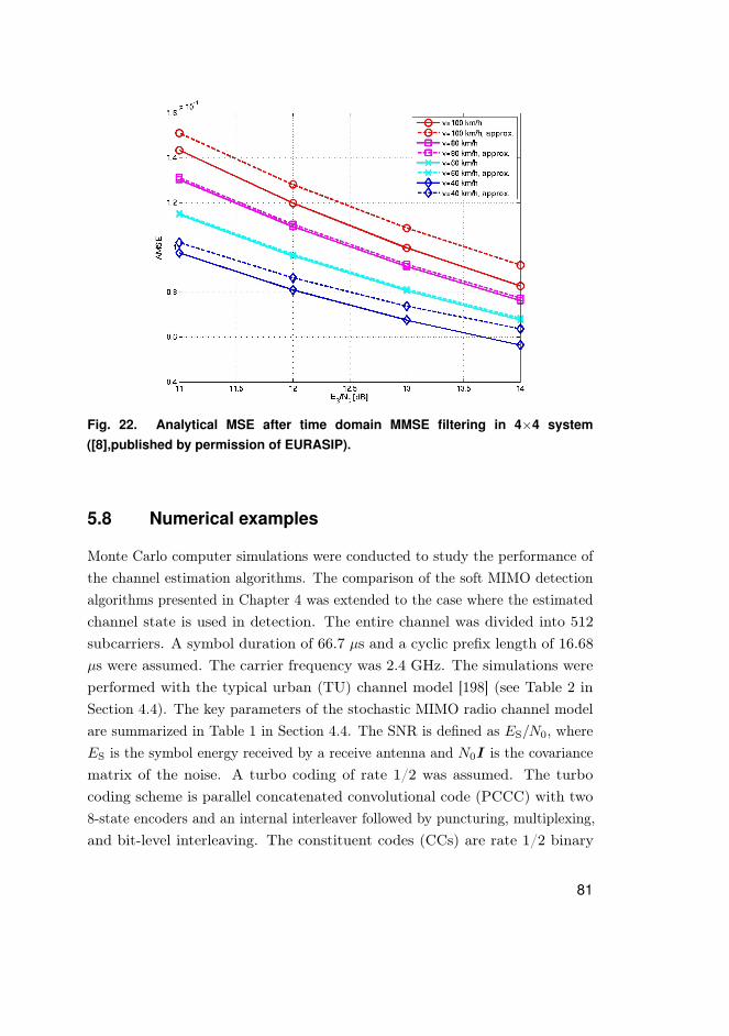
Fig. 22. Analytical MSE after time domain MMSE filtering in 4×4 system([8],published by permission of EURASIP).


Monte Carlo computer simulations were conducted to study the performance ofthe channel estimation algorithms. The comparison of the soft MIMO detectionalgorithms presented in Chapter 4 was extended to the case where the estimatedchannel state is used in detection. The entire channel was divided into 512subcarriers. A symbol duration of 66.7 µs and a cyclic prefix length of 16.68µs were assumed. The carrier frequency was 2.4 GHz. The simulations wereperformed with the typical urban (TU) channel model [198] (see Table 2 inSection 4.4). The key parameters of the stochastic MIMO radio channel modelare summarized in Table 1 in Section 4.4. The SNR is defined as ES/N0, whereES is the symbol energy received by a receive antenna and N0I is the covariancematrix of the noise. A turbo coding of rate 1/2 was assumed. The turbocoding scheme is parallel concatenated convolutional code (PCCC) with two8-state encoders and an internal interleaver followed by puncturing, multiplexing,and bit-level interleaving. The constituent codes (CCs) are rate 1/2 binary

81

recursive systematic convolutional codes [197]. The turbo decoder consists oftwo component MAP decoders [138] and 8 decoder iterations were performed.

5.8.1 Comparison of channel estimation algorithms

The mean square error (MSE) performance of the TD-SAGE channel estimatoris compared to that of the FD-SAGE and LS channel estimators in 2× 2 and4× 4 antenna configurations in Figs. 23 and 24, respectively. In addition, theperformance of the SAGE estimator in the simplified form as in (23) is given toshow the loss due to the simplification with non-constant envelope constellations.For the SAGE estimators, the MSE is given after the first and third iterations. Inthese cases, the known transmitted symbols are used in the estimation in orderto evaluate the channel estimation performance excluding error propagation,and the previous channel estimate is used to initialize the SAGE algorithms.64QAM and a mobile speed of 120 km/h are assumed. One can note that aloss of about 5 dB is caused in MSE in the 2× 2 antenna configuration if theFD-SAGE channel estimator is used in simplified form. In the 4× 4 antennaconfiguration, the loss of the simplified FD-SAGE channel estimator is 6.5 dB.The TD-SAGE channel estimator gives practically the same performance as theFD-SAGE channel estimator in general form with lower complexity in bothantenna configurations. The results indicate that just one channel estimatoriteration is enough if the system operation point is below 20 dB in both antennaconfigurations. One can note from Fig. 24 that three iterations for the TD-SAGEand FD-SAGE channel estimators are not enough to achieve LS performancebeyond 30 dB in the 4× 4 antenna configuration. However, this is not a practicaloperation area in most of the cases.

82

0 5 10 15 20 25 30 35 4010−5

10−4

10−3

10−2

10−1

100

ES/N0 [dB]

MSE

LSTD−SAGE 1 iterat.TD−SAGE 3 iterat.gen. FD−SAGE 1 iterat.gen. FD−SAGE 3 iterat.simp. FD−SAGE 1 iterat.simp. FD−SAGE 3 iterat.

Fig. 23. MSE performance in TU channel with 64QAM (2×2) ([4],published by per-mission of IEEE).

0 5 10 15 20 25 30 35 4010−5

10−4

10−3

10−2

10−1

100

101

ES/N0 [dB]

MSE

LSTD−SAGE 1 iterat.TD−SAGE 3 iterat.gen. FD−SAGE 1 iterat.gen. FD−SAGE 3 iterat.simp. FD−SAGE 1 iterat.simp. FD−SAGE 3 iterat.

Fig. 24. MSE performance in TU channel with 64QAM (4×4) ([4],published by per-mission of IEEE).

83

The FER performance results for the SAGE estimators with 16QAM and64QAM are presented in Fig. 25. With frame error, we refer to an erroneouscode word. Here, the detected and decoded data symbols are used in the channelestimation. Only one iteration is performed between the soft MIMO detector andthe turbo decoder. The IR-LSD [193] was operating as a soft MIMO detector.Only every 25th OFDM symbol was a preamble symbol, meaning that for every25th OFDM symbol all the sub-carriers from all the transmit antennas are usedfor pilot transmission. The channel estimate for the previous OFDM symbol isused to initialize the SAGE channel estimators. A mobile speed of 50 km/h wasassumed. It can be seen that the FD-SAGE channel estimator in the generalform and the TD-SAGE channel estimator exhibit approximately the sameperformance. The FD-SAGE channel estimator in the simplified form losesapproximately 1 dB in 16QAM case and about 2 dB in 64QAM case to thegeneral FD-SAGE and TD-SAGE channel estimators. The TD-SAGE andgeneral form FD-SAGE channel estimators lose around 2 dB in the 16QAM andclose to 4 dB in the 64QAM when compared to the performance with ideal CSIin the receiver. The preamble-based LS estimator with time domain MMSEpost-processing is presented as well. The preamble-based channel estimationsuffers from saturation in the performance due to the low preamble density.

84

16 18 20 22 24 26 28 30 32 3410−2

10−1

100

ES/N0 [dB]

FER

Ideal CSITD−SAGEgen. FD−SAGEsimp. FD−SAGEPreamble based

16QAM64QAM

Fig. 25. FER performance in TU channel with 16QAM and 64QAM (2×2) (4×4)([4],published by permission of IEEE).

Fig. 26 shows a performance comparison between the decision directedchannel estimation based on the SAGE algorithm and the preamble based LSestimator with time domain MMSE post-processing. The preamble overhead is4%. The list PIC detector is used as a soft MIMO detector with a list size of 4in the case of QPSK modulation and a list size of 8 in the case of 16-QAM. Thesuperiority of the SAGE based channel estimator can be clearly seen from theresults. The preamble based channel estimation suffers from saturation in theperformance due to low preamble density. Both of the estimators are furthercompared in Fig. 27, which shows the required pilot overhead versus the SNR toachieve the FER target of 10−1. Also the preamble based LS estimator withouttime domain processing is included in the figure. The results show that a hugeimprovement in spectral efficiency can be attained with DD channel estimation.The preamble overhead can be decreased from 17% to 4%, losing only 0.2 dBin performance and with a 0.5 dB loss in performance, overhead under 1% isachievable.

85

8 10 12 14 16 18 20 2210−2

10−1

100

ES/N0 [dB]

FER

SAGE, QPSK, list size 4, 1 GISAGE, QPSK, list size 4, 5 GIMMSE, QPSK, list size 4, 1 GIMMSE, QPSK, list size 4, 5 GISAGE, 16QAM, list size 8, 1 GISAGE, 16QAM, list size 8, 5 GIMMSE, 16QAM, list size 8, 1 GIMMSE, 16QAM, list size 8, 5 GI

Fig. 26. FER performance comparison between decision directed and pilot basedchannel estimation in typical urban channel (4×4) ([1],published by permission ofIEEE).

8.5 9 9.5 10 10.5 11 11.5 12 12.5 130

2

4

6

8

10

12

14

16

18

20

ES/N0 [dB]

Prea

mbl

e ov

erhe

ad [%

]

SAGE, QPSK, list size 4, 5 GIMMSE, QPSK, list size 4, 5 GILS, QPSK, list size 4, 5 GI

Fig. 27. Pilot overhead comparison between decision directed and pilot basedchannel estimation in typical urban channel with FER target of 10% (4×4)([1],published by permission of IEEE).

86

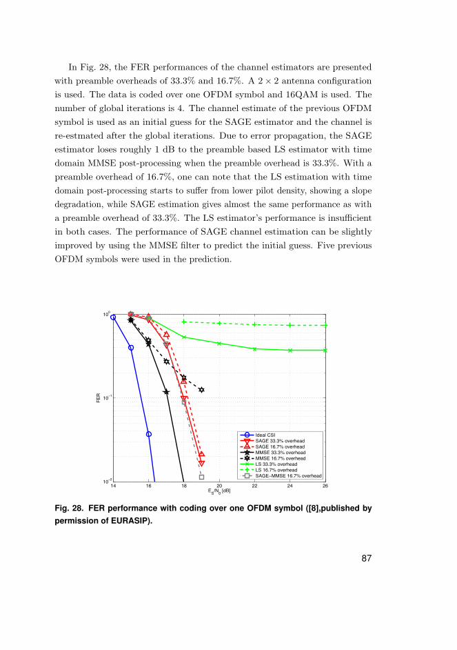
In Fig. 28, the FER performances of the channel estimators are presentedwith preamble overheads of 33.3% and 16.7%. A 2× 2 antenna configurationis used. The data is coded over one OFDM symbol and 16QAM is used. Thenumber of global iterations is 4. The channel estimate of the previous OFDMsymbol is used as an initial guess for the SAGE estimator and the channel isre-estmated after the global iterations. Due to error propagation, the SAGEestimator loses roughly 1 dB to the preamble based LS estimator with timedomain MMSE post-processing when the preamble overhead is 33.3%. With apreamble overhead of 16.7%, one can note that the LS estimation with timedomain post-processing starts to suffer from lower pilot density, showing a slopedegradation, while SAGE estimation gives almost the same performance as witha preamble overhead of 33.3%. The LS estimator’s performance is insufficientin both cases. The performance of SAGE channel estimation can be slightlyimproved by using the MMSE filter to predict the initial guess. Five previousOFDM symbols were used in the prediction.

14 16 18 20 22 24 2610−2

10−1

100

ES/N0 [dB]

FER

Ideal CSISAGE 33.3% overheadSAGE 16.7% overheadMMSE 33.3% overheadMMSE 16.7% overheadLS 33.3% overheadLS 16.7% overheadSAGE−MMSE 16.7% overhead

Fig. 28. FER performance with coding over one OFDM symbol ([8],published bypermission of EURASIP).

87

In Fig. 29, the data is encoded over 12 OFDM symbols and a preambleoverhead of 16.7% is assumed. The studied antenna configuration is 2× 2. Thenumber of global iterations is 4. The performance of LS estimation with timedomain MMSE post-processing is presented. In addition, the result in whichthe SAGE estimator is used to re-estimate the channel state after 2 globaliterations is shown. One can note that using the SAGE estimator within theglobal iterations degrades the performance slightly. When the channel coding isover multiple OFDM symbols, the refined channel estimate does not improve thesymbol decisions on a symbol-by-symbol basis. Thus, the erroneous symboldecisions deteriorate the SAGE channel estimates. To verify this, the resultsin which known symbols are used in SAGE estimation are presented. Fromthe results, one can see that ideally SAGE estimation could provide slightlyimproved performance. Also, if the number of global iterations, when the SAGEchannel estimator is activated, would be chosen in a more sophisticated manneras discussed in Chapter 6, the results might be improved.

14 14.5 15 15.5 16 16.5 17 17.5 1810−2

10−1

100

ES/N0 [dB]

FER

Ideal CSIMMSE−SAGEMMSEMMSE−SAGE genie aided

Fig. 29. FER performance with coding over 12 OFDM symbols ([8],published bypermission of EURASIP).

88

Figs. 30 and 31 show the FER performances after MMSE filtering in 2× 2

and 4× 4 antenna configurations and with QPSK and 16QAM, respectively. Theframe length is 6 OFDM symbols and the channel coding is over one frame. TheIR-LSD [193] was operating as the soft MIMO detector. The results with twopre-caluculated filters (MMSE approximations) are compared to those given bythe filters calculated using the ideal channel parameters. A mobile speed of 85km/h was assumed in the pre-calculated filter for true mobile speeds of 100km/h and 80 km/h while a mobile speed assumption of 55 km/h was used in thepre-calculated filter for true mobile speeds of 40 km/h and 60 km/h. The fixedSNR values were 8.6 dB and 11.4 dB in the case of QPSK in 2× 2 and 4× 4

antenna configurations, respectively, while in the case of 16QAM, they were 17.4dB and 21.7 dB. The results clearly show that in the presented cases, MMSEfiltering can be approximated with two pre-calculated filters with insignificantloss, and in a 2× 2 antenna configuration, even one pre-calculated filter mightbe sufficient.

! " # $% $$ $& $' $(

$%!$

$%%

)*+,%-./01

2)3

-

-

44*)-$%%-56+7

44*)-"%-56+7

44*)-8%-56+7

44*)-(%-56+7

44*)-9::3;-$%%-56+7

44*)-9::3-"%-56+7

44*)-9::3;-8%-56+7

44*)-9::3;-(%-56+7

(-!-(&-!-&

Fig. 30. Performance of pre-calculated MMSE filters in 2×2 and 4×4 antenna con-figurations assuming QPSK ([8],published by permission of EURASIP).

89

!" !# !$ !% &' &! && &( &) &*

!'!!

!''

+,-.'/0123

4+5

/

/

66,+/!''/78-9

66,+/$'/78-9

66,+/"'/78-9

66,+/)'/78-9

66,+/:;;5</!''/78-9

66,+/:;;5</$'/78-9

66,+/:;;5</"'/78-9

66,+/:;;5</)'/78-9

&/!/& )/!/)

Fig. 31. Performance of pre-calculated MMSE filters in 2×2 and 4×4 antenna con-figurations assuming 16QAM ([8],published by permission of EURASIP).

5.8.2 Comparison of soft MIMO detection algorithms withestimated channel

The list PIC detector was compared to the APP algorithm, the K-best LSD,and the IR-LSD when operating as the soft MIMO detector with estimatedchannel state information. The FER performance of the detectors is presentedfor QPSK, 16QAM, and 64QAM constellations and for 2× 2 and 4× 4 antennaconfigurations. The SAGE algorithm is used in decision directed mode totrack the channel on a symbol-by-symbol basis after the preamble based LSinitialization and the coding is over one OFDM symbol.

From Fig. 32, one can note that with a list size of four, the list PIC algorithmloses insignificantly to the APP algorithm when QPSK is considered as themodulation scheme and Mt = Mr = 2. The K-best LSD and the IR-LSDoffer exactly the same performance as the list PIC detector with the list sizeof four (not shown in the figure). When a list size of two is used, the listdetectors are outperformed by the APP algorithm. However, the performance

90

degradation of the K-best LSD is more than that of the list PIC detector, whilethe IR-LSD outperforms both of the other list detectors. With QPSK, the SAGEchannel estimator can be used in the simplified form and the loss due to thechannel estimation seems to be around 2 dB when these results are comparedto the corresponding results with ideal channel state information presented inChapter 4.

8 10 12 14 16 18 2010−2

10−1

100

ES/N0 [dB]

FER



The simulation results assuming 16QAM and Mt = Mr = 2 are presented inFig. 33. A list size of 16 gives optimal performance with all the list detectorsand has been excluded from the figure. The superiority of the list PIC detectorover the K-best LSD can be seen with a list size of 8. However, the IR-LSDoutperforms the list PIC detector, gaining about 0.5 dB. The loss in performancedue to channel estimation is around 2 dB with the general SAGE estimator andwith the simplification approximately 2.5 dB.

91

16 16.5 17 17.5 18 18.5 19 19.5 20 20.5 2110−2

10−1

100

ES/N0 [dB]

FER

APP 1 GIAPP 5 GIAPP 1 GI simp. SAGE8−List PIC 1 GI8−List PIC 5 GI8−Kbest 5 GI8−IR−LSD 5 GI


The performance of the APP algorithm is not simulated for the 64QAM casein a 2× 2 antenna configuration due to the computational complexity of sucha simulation. Instead, the list PIC detector with a list size of 256 is used asa reference in Fig. 34. The performance of the list PIC detector deterioratesinsignificantly when the list size is decreased to 32, while the performance losswith the K-best LSD is more noticeable. The superiority of the list PIC detectorover the K-best LSD is further emphasized with a list size of 16 in this case.The IR-LSD offers practically the same performance with the list size of 16 asthe list PIC detector with a list size of 32. The channel estimation loss is around3 dB with the SAGE estimator, whereas with simplification the loss is close to 6dB. One should also note the slope degradation in FER with 1 GI in this case.It is caused by error propagation. Within the presented examples, at least 1 dBof gain is achieved by exchanging the extrinsic information between the detectorand the decoder. In the case of 64QAM, the gain is closer to 2 dB.

92

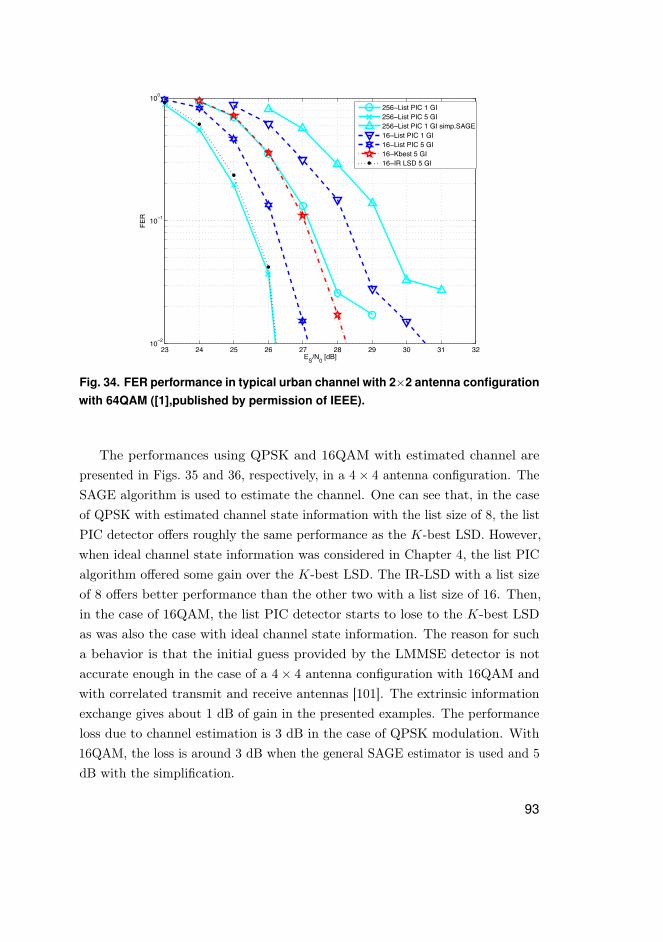
23 24 25 26 27 28 29 30 31 3210−2

10−1

100

ES/N0 [dB]

FER

256−List PIC 1 GI256−List PIC 5 GI256−List PIC 1 GI simp.SAGE16−List PIC 1 GI16−List PIC 5 GI16−Kbest 5 GI16−IR LSD 5 GI


The performances using QPSK and 16QAM with estimated channel arepresented in Figs. 35 and 36, respectively, in a 4× 4 antenna configuration. TheSAGE algorithm is used to estimate the channel. One can see that, in the caseof QPSK with estimated channel state information with the list size of 8, the listPIC detector offers roughly the same performance as the K-best LSD. However,when ideal channel state information was considered in Chapter 4, the list PICalgorithm offered some gain over the K-best LSD. The IR-LSD with a list sizeof 8 offers better performance than the other two with a list size of 16. Then,in the case of 16QAM, the list PIC detector starts to lose to the K-best LSDas was also the case with ideal channel state information. The reason for sucha behavior is that the initial guess provided by the LMMSE detector is notaccurate enough in the case of a 4× 4 antenna configuration with 16QAM andwith correlated transmit and receive antennas [101]. The extrinsic informationexchange gives about 1 dB of gain in the presented examples. The performanceloss due to channel estimation is 3 dB in the case of QPSK modulation. With16QAM, the loss is around 3 dB when the general SAGE estimator is used and 5dB with the simplification.

93

11 11.5 12 12.5 13 13.5 14 14.5 15 15.5 1610−2

10−1

100

Es/N0 [dB]

FER

APP 1 GI APP 5 GI 16−List PIC 1 GI16−List PIC 5 GI16−Kbest 5 GI8−List PIC 1 GI8−List PIC 5 GI8−Kbest 5 GI8−IR−LSD 5 GI


21 22 23 24 25 26 27 2810−2

10−1

100

ES/N0 [dB]

FER

256−Kbest 1 GI256−Kbest 5 GI256−Kbest 1 GI simp. SAGE256−List PIC 1 GI256−List PIC 5 GI64−Kbest 5 GI32−IR−LSD 5 GI


94


Decision directed (DD) and iterative channel estimation were compared topreamble based channel estimation in an iterative receiver composed of a softMIMO detector, a channel estimator, and a turbo decoder in MIMO-OFDMsystems. The conventional LS estimator operating in DD mode requires inversionof a matrix with the size per dimension dependent on the number of transmitantennas and the length of the channel impulse response. The matrix inversioncan be avoided with the FD-SAGE channel estimator with constant envelopemodulation. However, the drawback with the FD-SAGE channel estimatoris the required inversion of a matrix of a size depending on the length of thechannel impulse response when non-constant envelope constellations are used.The TD-SAGE estimator was derived to lower the complexity by avoiding thematrix inversion without performance degradation.

The performance and complexity of the DD SAGE channel estimators werecompared to that of the preamble based LS channel estimator with and withoutMMSE post-processing, using various preamble densities. According to theresults, the use of DD SAGE channel estimation is beneficial if the channelcoding is over one OFDM symbol and with preamble overheads less than 16.7%.Despite the fast fading channel, it was possible to decrease the preamble overheadfrom 17% to 4% losing only 0.2 dB in the performance, and with a 0.5 dB lossin performance overhead under 1% was achievable with DD SAGE channelestimation. The decrease in preamble overhead was achieved by increasedcomplexity in channel estimation. The SAGE estimator performance was furtherimproved by using the MMSE filter and the previous channel estimates topredict the initial guess. The re-estimation of the channel state within theglobal iterations, i.e., iterative channel estimation, did not give any gain inthe studied cases. However, there was no tool to adapt the activation scheduleof the channel estimation for instantaneous channel state. Thus, one cannotsay that there is no gain to be achieved by using iterative channel estimation.Instead, this is taken into closer consideration in Chapter 6. The architectureexamples were presented for the preamble based LS estimator and the FD-SAGEestimator assuming constant envelope constellation. It was also shown that thetime correlation of the channel can be exploited by MMSE filtering to improve

95

the channel estimation performance with only a small increase in complexity byusing few pre-calculated filters.

The list detector study provided in Chapter 4 was extended for the case ofan estimated channel. The results were well aligned with those obtained withthe ideal channel state information in the receiver in Chapter 4. The list PICdetector offers close to optimal performance with reduced complexity and aperformance gain over the K-best LSD with proper initialization. The LMMSEproved to be good enough in the initialization in a 2× 2 antenna configuration,but in a 4 × 4 antenna configuration with higher order modulations, it wasinadequate. The IR-LSD offered performance gain over the other studied listdetectors. However, in the case of a 2× 2 antenna configuration, the gain overthe list PIC detector was not substantial.

96

6 Scheduling of activations in iterativedetection, decoding, and channel estimationfor MIMO-OFDM

The purpose of this chapter is to present a framework for the activation schedulingof a soft MIMO detector, a channel decoder, and a channel estimator. In aniterative receiver with two SfISfO blocks, the two blocks are activated in turns.With more than two SfISfO blocks, the schedule of activations is no longerobvious. EXIT charts together with a trellis search algorithm are used hereas a tool to find out the optimal activation schedule for the SfISfO blocks.Conventionally, EXIT analysis has been used to study the convergence propertiesof iterative receivers in such a way that the equalizer and channel estimatorare considered as a single SfISfO block [185][186][187]. However, this providesno information regerding the individual performance of the estimator and theequalizer. Our concept is inspired by [188] and assumes the separation of thedetector and channel estimator activations.

EXIT charts have been used to organize efficient activation scheduling forconcatenated codes [181][182], multiuser detectors and turbo decoder iterations[183]. More specifically, the authors in [183] optimize the number of turbodecoder iterations for different users in CDMA uplink in an AWGN channel.In this chapter, the activation schedule for a soft MIMO detector, a channeldecoder, and a channel estimator in a multipath channel is optimized. Thechannel estimator brings the third dimension into the activation schedulingproblem, complicating the problem a bit. The main contributions of the chapterare as follows. A semi-analytical method to generate the EXIT function forthe least-squares channel estimator in MIMO-OFDM systems is derived. Thederivation is based on the assumption that the multipath channel between eachantenna pair is considered as a set of parallel channels with colored Gaussiannoise. An algorithm is proposed to generate the EXIT function for the softMIMO detector as a function of the mutual information between the channelestimate and the true channel state. We show that the analytical expressions forthe EXIT function of the soft MIMO detector and the decoder can be found by

97

fitting the measured functions to the third order surface and curve, respectively.Inspired by [182], we propose trellis search based algorithms which use theEXIT functions to find the activation order which minimizes the complexity andguarantees convergence, if there is an opening between the EXIT functions.

The rest of the chapter is organized as follows. Section 6.1 introduces thedefinition of mutual information (MI) and EXIT charts as tools to analyze theconvergence behavior of iterative receivers. Section 6.2 formulates the activationscheduling problem more specifically. In Section 6.3, the generation of theEXIT functions is discussed. Trellis search based algorithms which use theEXIT functions to find the activation order are presented in Section 6.4. Someperformance examples with the proposed activation scheduling framework arepresented in Section 6.5. Finally, conclusions are drawn in Section 6.6.

6.1 Mutual information and extrinsic information charts

An EXIT chart describes the convergence of the iterative algorithm by investigat-ing the exchange of mutual information (MI) [38] between the SfISfO components.The MI of two random variables is a quantity that measures the mutual de-pendence of the two variables. Intuitively, MI tells how much information onevariable carries about the other variable, i.e., how much knowledge about one ofthe variables reduces uncertainty about the other.

Let us consider iterative processing between a soft MIMO detector and achannel decoder, illustrated in Fig. 1 in Section 3.3, as an example. The mutualinformation between the extrinsic LLRs and the transmitted bits at the outputof the detector Mdet

E and the decoder MdecE is defined as [174]

ME =

1

2

∑b=−1,+1

∫ +∞

−∞p(LE |B = b) log2

(2p(LE |B = b)

p(LE |B = −1) + p(LE |B = +1)

)dLE ,

(40)

where B is the transmitted data, and p(LE |B = b) is the probability densityfunction (PDF) of the output extrinsic LLRs conditioned on the transmittedcode bit b. The range of Mdet

E and MdecE is [0, 1], where Mdet

E = 0 or MdetE = 1

correspond, respectively, to no or perfect knowledge about b given the LLRs. Ifthe symmetry constraint p(LE |B = b) = p(−LE |B = −b) holds, (40) simplifies

98

to

ME =

∫ +∞

−∞p(LE |B = 1) log2

(2p(LE |B = 1)

p(LE |B = 1) + p(−LE |B = 1)

)dLE . (41)

The integrals in (40) and (41) can be numerically calculated from the conditionalPDFs, which are estimated by histogram measurements.

An EXIT function describes the transformation of the input a priori mutualinformation into the output extrinsic mutual information. For the soft MIMOdetector and the decoder, the EXIT functions are defined as

T det : MdetA,dec → T det(Mdet

A,dec|σ2w ,hmr), mr = 1, ...,Mr (42)

T dec : MdecA,det → T dec(Mdec

A,det), (43)

respectively, where MdetA,dec = Mdec

E and MdecA,det = Mdet

E . The EXIT functions arevalid definitions of the input-output characteristics for the case of infinite blocklength, but with finite block lengths, the input-output characteristic acquires arandom variation around the asymptote [180]. In general, the EXIT functionsare assumed to be monotonically increasing, i.e., increasing a priori informationincreases output mutual information. The case of a flat EXIT function indicatesindependence between the a priori information and the value being estimated.The EXIT function of the decoder is relatively straightforward to evaluate as itis fixed. Analytical computation of the decoder EXIT function is currently notknown for the channel codes over Gaussian channels. In addition, in this thesis,the EXIT functions of channel decoders are generated through simulations.The decoder EXIT function is specific to the decoding algorithm, code rate,interleavers, and code polynomials. The EXIT function of the detector dependson the channel state, SNR value, and the detection algorithm.

The EXIT chart is a plot including the MI transfer functions of all thereceiver components. The purpose of the EXIT chart is to predict the trajectoryfrom the mutual information transfer functions of SfISfO blocks. The evolutionof Mdet

E and MdecE over the iterations in a receiver is referred to the trajectory of

the iterative algorithm. The trajectory reveals the convergence properties of theiterative algorithm. At the ith iteration, the soft MIMO detector output mutualinformation is given by the recursion

MdetE (i) = T det(T dec(Mdet

E (i− 1))). (44)

99

After combining the soft MIMO detector function and the decoder function intoone EXIT chart, the convergence of the algorithm can be tracked by invoking theiteration (44). The functions are arranged such that the output of one componentshares an axis with the corresponding input of the component to which it isconnected. The process in our example is illustrated with hypothetical detectorand decoder EXIT functions in Fig. 37. The process begins with no a prioriinformation at (M

(det)E = 0,M

(det)E = 0), followed by alternating activations of

the soft MIMO detector and the decoder performing the convergence steps untilthe point where the exit functions of the detector and decoder cross, or thepoint of error-free decoding (M

(det)E = 1,M

(det)E = 1) is reached. A vertical line

represents detector activation, and a horizontal line is for decoder activation. Tolet the iterations to continue and errors be minimized, there must be an openingin the EXIT chart between the detector and decoder functions. More precisely,the constraint

T det(MdecE )− T det−1

(MdecE ) > 0, ∀Mdec

E ∈ [0, 1] (45)

must be fulfilled. As seen in Fig. 37, the detector EXIT function fulfills theconstraint and the convergence point 1, 1 is reached, which means thaterror-free decoding is achieved.

100

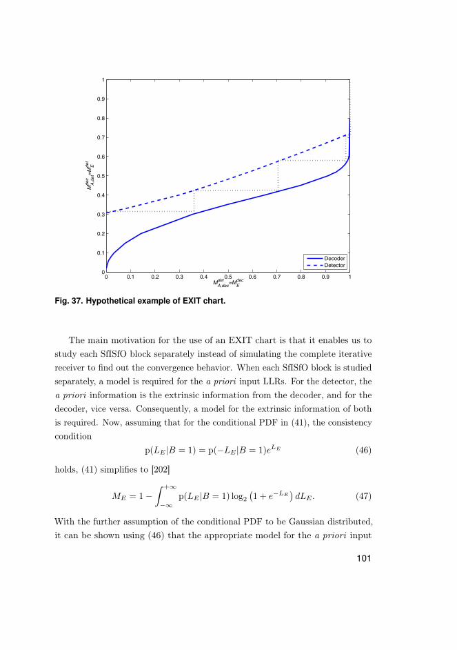
0 0.1 0.2 0.3 0.4 0.5 0.6 0.7 0.8 0.9 10

0.1

0.2

0.3

0.4

0.5

0.6

0.7

0.8

0.9

1

MA,decdet =ME

dec

MA,det

dec=M

Edet

DecoderDetector

Fig. 37. Hypothetical example of EXIT chart.

The main motivation for the use of an EXIT chart is that it enables us tostudy each SfISfO block separately instead of simulating the complete iterativereceiver to find out the convergence behavior. When each SfISfO block is studiedseparately, a model is required for the a priori input LLRs. For the detector, thea priori information is the extrinsic information from the decoder, and for thedecoder, vice versa. Consequently, a model for the extrinsic information of bothis required. Now, assuming that for the conditional PDF in (41), the consistencycondition

p(LE |B = 1) = p(−LE |B = 1)eLE (46)

holds, (41) simplifies to [202]

ME = 1−∫ +∞

−∞p(LE |B = 1) log2

(1 + e−LE

)dLE . (47)

With the further assumption of the conditional PDF to be Gaussian distributed,it can be shown using (46) that the appropriate model for the a priori input

101

LLRs is expressed as

LA = µAb+ nA, (48)

where b is the transmitted bit, nA is a Gaussian random variable with zeromean and variance σ2

A and µA =σ2A

2 . This means that the conditional PDF is afunction of the variance of the input LLRs and the mutual information itself is afunction of variance and given by

MA(σA) = J(σA) = 1−∫ +∞

−∞

exp(−(LA−σ2

A/2)2

2σ2A

)√

2πσ2A

log2(1 + e−LA)dLA. (49)

Consequently, (49) gives the mapping between the a priori mutual informationMA and σA and is called the J-function. With the J-function, one can getthe variance to generate the a priori LLRs corresponding to certain mutualinformation. There is no closed form expression for the J-function or itsinverse under the Gaussian assumption, but accurate approximations have beendeveloped. One approximation is [182]

MA = J(σA) ≈ (1− 2−S1σ2S2A )S3 (50)

and its inverse

σA = J−1(MA) ≈(− 1

S1log2(1−MA

1S3 )

) 12S3

, (51)

where S1 = 0.3073, S2 = 0.8935, and S3 = 1.1064.Beside being useful in EXIT chart derivation, the J-function also provides an

easy means for estimating the bit error rate (BER). The a posteriori output ofthe decoder can be written as LD = LA + LE . Under the assumption that bothLA and LE are Gaussian distributed, the a posteriori output is also Gaussian.Since hard decisions are made on the a posteriori output, the BER can beestimated as [174]

Pb ≈ Q(σD2

), (52)

where Q(·) is the integral of the tail of a zero-mean Gaussian PDF with varianceone and σ2

D is the variance of LD. Assuming LA and LE to be independent, thevariance of LD is given by

σ2D = σ2

A + σ2E . (53)

102

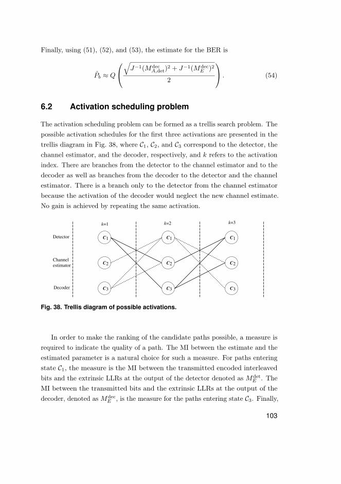
Finally, using (51), (52), and (53), the estimate for the BER is

Pb ≈ Q

√J−1(Mdec

A,det)2 + J−1(Mdec

E )2

2

. (54)

6.2 Activation scheduling problem

The activation scheduling problem can be formed as a trellis search problem. Thepossible activation schedules for the first three activations are presented in thetrellis diagram in Fig. 38, where C1, C2, and C3 correspond to the detector, thechannel estimator, and the decoder, respectively, and k refers to the activationindex. There are branches from the detector to the channel estimator and to thedecoder as well as branches from the decoder to the detector and the channelestimator. There is a branch only to the detector from the channel estimatorbecause the activation of the decoder would neglect the new channel estimate.No gain is achieved by repeating the same activation.

C1

C2

C3

C1 C1

C2 C2

C3 C3

k=1 k=2 k=3

Detector

Channelestimator

Decoder

Fig. 38. Trellis diagram of possible activations.

In order to make the ranking of the candidate paths possible, a measure isrequired to indicate the quality of a path. The MI between the estimate and theestimated parameter is a natural choice for such a measure. For paths enteringstate C1, the measure is the MI between the transmitted encoded interleavedbits and the extrinsic LLRs at the output of the detector denoted as Mdet

E . TheMI between the transmitted bits and the extrinsic LLRs at the output of thedecoder, denoted as Mdec

E , is the measure for the paths entering state C3. Finally,

103

the paths entering state C2 are ranked using the MI between the actual channelstate and the channel estimate denoted as Mh. Each activated component usesthe information provided the other two components. Consequently, mappingfrom the MI provided by the other two components to the MI at the outputof the activated component is needed. This mapping is given by the EXITfunctions.

The particular activation order determines the cost of convergence. Theterm “cost” can, for example, refer to computational complexity, latency, orpower consumption. Evidently, it is of interest to reach the convergence targetwith the lowest possible cost. Let us here define optimal activation schedulingto be scheduling which reaches the convergence target with the lowest totalcomputational complexity c. In other words, based on the EXIT functions, noother activation order can reach the convergence target with lower complexity.Yet, one should note that this thesis does not even try to define the exactcost values of SfISfO blocks, but rather a framework for activation schedulingembracing the computational cost is presented and its impact is examined. Inthe following, we first present the methods to generate the EXIT functions forthe SfISfO components and then discuss the trellis search algorithms to find theoptimal activation schedule.

6.3 EXIT chart analysis

This section provides EXIT chart analysis for the LS channel estimator, the APPalgorithm, and the RA decoder. For all these cases, the a priori informationis assumed to be Gaussian distributed satisfying the consistency requirement[174] and is modeled as in (48). The mapping between the a priori mutualinformation MA and σA is given by the approximated J-function in (50).

6.3.1 EXIT function for LS channel estimator

The DD LS channel estimate can be presented as

hmr= (GHG)−1GHXF︸︷︷︸

A

hmr+ (GHG)−1GH︸︷︷︸

B

wmr, (55)

104

where G = XF . Then, by adding and subtracting hmr, the LS estimate becomes

hmr= hmr

+(

(GHG)−1GHXF − I)

︸︷︷︸D

hmr+ (GHG)−1GHwmr

︸︷︷︸wmr

. (56)

Thus, the LS estimate is the actual channel state plus some noise wmr(the last

two terms in (56)). In fact, according to computer simulations, the noise term foreach path closely follows Gaussian distribution. However, we cannot assume thenoise term to be uncorrelated over different paths. With these characteristics andconditioned on the true channel, the mutual information between the channelestimate and the actual channel state is [38, Chapt. 9]

Mh =1

2log2

|C ˆhmr

|

|Cwmr|, (57)

where

C ˆhmr

= Ewmr ,X ,ˆX (hmr

hHmr

) (58)

= EX ,ˆX (Ahmr

hHmr

AH + σ2wmr

BBH)

= EX ,ˆX

((FHX

HXF )−1FHX

HXFhmr

hHmr

FHXHXF (FHXH

×XF )−1 + σ2wmr

((FHX

HXF )−1FHX

HXF (FHX

HXF )−1

)),

Cwmr= Ewmr ,X ,

ˆX (wmrwHmr

) (59)

= EX ,ˆX (Dhmr

hHmr

DH + σ2wmr

BBH)

= EX ,ˆX

(((FHX

HXF )−1FHX

HXF − I

)hmr

hHmr

(FHXHXF

×(FHXHXF )−1 − I

)+ σ2

wmr

((FHX

HXF )−1FHX

HXF

×(FHXHXF )−1

)).

In (58) and (59), we end up calculating the expectations EX ,ˆX (X

HX ) and

EX ,ˆX (X

HX ) which are algebraically involved. The EXIT chart analysis

105

assumes that the interleaver block lengths are large and we also assumedthat modulation is memoryless. Therefore, the symbols and the tentativedecisions made become approximately independent. Numerical evaluations ofEX ,

ˆX (XHX ) verify the assumption and the covariance matrix can be assumed

to be diagonal. In Figs. 39 and 40, one can see the examples with low and high apriori mutual information values, respectively. Furthermore, in the case of hardsymbol estimates, the diagonal contains the expected power of the constellation,which was 2 in the examples. Consequently, the following approximation

EX ,ˆX (X

HX ) ≈ EX (XHX ) = EcI , (60)

where Ec is the expected power of the used constellation, can be done. Evidently,the cross covariance matrix of the symbol and symbol estimate matrices is diagonalas well due to the independency assumption. However, if there are decisionerrors, the diagonal does not contain the expected power of the constellation,but something less. This can be seen also in the numerical evaluations ofEX ,

ˆX (XHX ) in Figs. 41 and 42 with low and high a priori mutual information

values. For constant envelope constellation, the following approximation

EX ,ˆX (X

HX ) ≈ diag(X

HX ) (61)

provides a good result. Its validity was confirmed by computer simulations whichshowed a relatively good match between the semi-analytical and the measuredresults (See Fig. 43 in Section 6.5).

106

Fig. 39. Values of the elements of the estimated symbol decision auto-covariancematrix (Mh

A,det = MhA,dec = 0.1).

Fig. 40. Values of the elements of the estimated symbol decision auto-covariancematrix (Mh


107

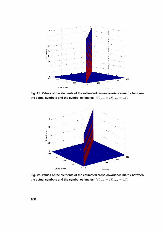
Fig. 41. Values of the elements of the estimated cross-covariance matrix betweenthe actual symbols and the symbol estimates (Mh


Fig. 42. Values of the elements of the estimated cross-covariance matrix betweenthe actual symbols and the symbol estimates (Mh


108

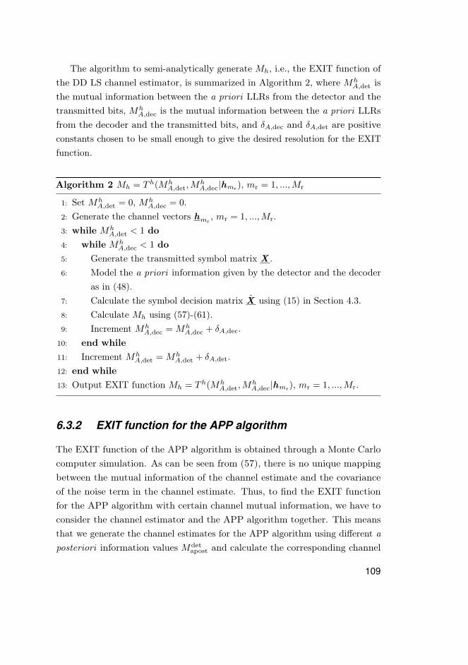
The algorithm to semi-analytically generate Mh, i.e., the EXIT function ofthe DD LS channel estimator, is summarized in Algorithm 2, where Mh

A,det isthe mutual information between the a priori LLRs from the detector and thetransmitted bits, Mh

A,dec is the mutual information between the a priori LLRsfrom the decoder and the transmitted bits, and δA,dec and δA,det are positiveconstants chosen to be small enough to give the desired resolution for the EXITfunction.

Algorithm 2 Mh = Th(MhA,det,M

hA,dec|hmr), mr = 1, ...,Mr

1: Set MhA,det = 0, Mh

A,dec = 0.2: Generate the channel vectors hmr

, mr = 1, ...,Mr.3: while Mh

A,det < 1 do4: while Mh

A,dec < 1 do5: Generate the transmitted symbol matrix X .6: Model the a priori information given by the detector and the decoder

as in (48).7: Calculate the symbol decision matrix X using (15) in Section 4.3.8: Calculate Mh using (57)-(61).9: Increment Mh

A,dec = MhA,dec + δA,dec.

10: end while11: Increment Mh

A,det = MhA,det + δA,det.

12: end while13: Output EXIT function Mh = Th(Mh

A,det,MhA,dec|hmr), mr = 1, ...,Mr.

6.3.2 EXIT function for the APP algorithm

The EXIT function of the APP algorithm is obtained through a Monte Carlocomputer simulation. As can be seen from (57), there is no unique mappingbetween the mutual information of the channel estimate and the covarianceof the noise term in the channel estimate. Thus, to find the EXIT functionfor the APP algorithm with certain channel mutual information, we have toconsider the channel estimator and the APP algorithm together. This meansthat we generate the channel estimates for the APP algorithm using different aposteriori information values Mdet

apost and calculate the corresponding channel

109

mutual information value. Note that the decoder a priori information MdetA,dec is

independently generated from Mdetapost.

After generating the histograms to estimate the conditional PDF of theextrinsic LLRs LE , Pr(LE |b = ±1) with different a priori values from thedecoder and with different channel estimate mutual information values, themutual information between the LLRs and the transmitted bits is calculated asin (40). The algorithm to simulate the EXIT function of the APP algorithmparametrized with the decoder a priori information and the channel estimatemutual information is summarized in Algorithm 3.

Algorithm 3 MdetE = T det(Mh,M

detA,dec|σ2w ,hmr) mr = 1, ...,Mr

1: Set Mdetapost = 0, Mdet

A,dec = 0.2: Generate the channel vectors hmr

, mr = 1, ...,Mr.3: while Mdet

apost < 1 do4: while Mdet

A,dec < 1 do5: Generate the transmitted symbol matrix X .6: Generate the received signal vectors ymr

, mr = 1, ...,Mr.7: Generate the symbol decisions corresponding to Mdet

apost.8: Estimate the channel using (16) and measure C ˆh and Cw and calculate

Mh by (57).9: Model the a priori input to the detector as in (48).

10: Activate the APP algorithm.11: Generate the histograms to estimate the conditional PDF of LE ,

Pr(LE |b = ±1) and use (40) to calculate the MI.12: Increment Mdet

A,dec = MdetA,dec + δA,dec.

13: end while14: Increment Mdet

apost = Mdetapost + δapost.

15: end while16: Output EXIT function Mdet

E = T det(Mh,MdetA,dec|σ2w ,hmr) mr = 1, ...,Mr.

A closed form expression for the EXIT function of the APP algorithm isrequired for scheduling the activations. An approximated analytical expressionfor the EXIT function can be found, for example, by fitting the surface to the

110

3rd order surface equation expressed as

MdetE = a30M

3h + a21M

2hM

detA,dec + a20Mh + a12MhM

det2A,dec (62)

+a11MhMdetA,dec + a10Mh + a03M

det3A,dec + a02M

det2A,dec + a01M

detA,dec + a00.

The 3rd order surface was chosen as the lowest possible order to keep thecomputational complexity of the surface fitting as simple as possible.

6.3.3 EXIT function for the RA decoder

The EXIT function of the RA decoder is obtained through a Monte Carlocomputer simulation. The mutual information between the LLRs and thetransmitted bits is given by (40) after generating the histogram estimates for theconditional PDFs. The algorithm to simulate the EXIT function of the decoderparametrized with the detector a priori information is given in Algorithm 4.

Algorithm 4 MdecE = T dec(Mdec

A,det)

1: Set MdecA,det = 0.

2: while MdecA,det < 1 do

3: Model the a priori input to the decoder as in (48).4: Activate the decoder.5: Generate the histograms to estimate the conditional PDF of LE , Pr(LE |b =

±1) and use (40) to calculate the MI.6: Increment Mdec

A,det = MdecA,det + δA,det.

7: end while8: Output EXIT function Mdec

E = T dec(MdecA,det).

The decoder EXIT function is independent of the channel state. Thus, anapproximated analytical expression for it can be found by fitting the curve tothe 3rd order polynomial given by

MdecE = a3M

dec3A,det + a2M

dec2A,det + a1M

decA,det + a0. (63)

The decoder EXIT function could also be calculated off-line and tabulated foractivation scheduling. The curve fitting is used here due to its straightforwardimplementation.

111

6.4 Trellis search for optimal activation order

The activation problem was formed as a trellis search problem in Section 6.2.This section provides two trellis search algorithms to find the optimal activationschedule under the monotonicity assumption of the EXIT functions. We defineak as a state at activation k, and ak = n corresponds to using Cn at the kthactivation. A path entering the state ak = n and corresponding to a specificactivation schedule is defined as pk = (p1, p2, .., pk), where pj ∈ 1, 2, 3 for1 ≤ j ≤ k− 1 and pk = n. Let v = (MD, c,M

detE ,Mh,M

decE ) be the metric vector

associated with the path, where MD is the convergence target, and c is the totalcomplexity resulting from activations along the path pk. The metric updatefunctions for the detector, the channel estimator and the decoder activations aregiven as

f1(v) = (v1, v2 + c1, Tdet(σw ,Mh,M

detA,dec), v4, v5) (64)

f2(v) = (v1, v2 + c2, v3, Th(Mh

A,dec,MhA,det), v5) (65)

f3(v) = (v1, v2 + c3, v3, v4, Tdec(Mdec

A,det)), (66)

respectively, where vn refers to nth element in v and cn is the complexity cost ofactivating Cn.

Let Pk ∈ IN and Vk ∈ IR+ be the sets of surviving paths and metrics afterk activations, respectively, and let Pk,n ⊆ Pk and Vk,n ⊆ Vk be the sets ofpaths and metrics entering state n after k activations. Similarly as in [182] forconcatenated channel codes, the exhaustive search for our purposes is describedin Algorithm 5.

112

Algorithm 5 Brute-Force Exhaustive Search1: Define p∗ and v∗ be a candidate path and metric with initial complexityv2 =∞ and let k = 1.

2: Initialize Pk = 1, and Vk = f1(v0) (detector has to be activated at first),where v0 = (MD, 0, 0,Mh, 0). (We have some initial guess of the channelstate in the beginning.)

3: while |Vk| 6= 0 do4: Increment k by one.5: For each state n′, extend every path p ′k−1 ∈ Pk−1,n′ with metric v ′, along

the possible state transitions n′ → n.6: Add the new paths pk = (p ′k−1, n) to Pk,n and the corresponding updated

metrics v = fn(v ′) to Vk,n.7: Reduce the set Vk to include metrics v ∈ Vk if v2 < v∗2 and reduce Pk

accordingly.8: Define a new set of metrics V∗ containing v ∈ Vk for which v3 ≥MD or

v5 ≥MD.9: If |V∗| 6= 0, find v∗ = arg minv∈V∗ v2, and replace p∗ by the path

corresponding to v∗.10: end while11: Output p∗ as the optimal path and corresponding metric vector v∗.

The number of paths grows exponentially with k until the first candidatepath is found when the brute-force algorithm is used. Consequently, if the EXITsurfaces are close to each other, the brute-force algorithm may be computationallytoo intensive. The complexity can be reduced by modifying the Viterbi algorithmin [182] for our purposes by deleting the paths entering the same state andhaving no impact on the final outcome. For that, we need the following definition[182].

Definition 1 (Domination): Define a partial ordering on Vk,n as follows. Forv , v ′ ∈ Vk,n, v v ′ if and only if vj ≥ v′j , j ∈ 3, 4, 5 and v2 ≤ v′2.

Let us define the function dom (operating on a set of metrics) to be a functionwhich discards the dominated metrics. Thus, Vk,n = domV ′k,n discards all

113

v ′ ∈ V ′k,n for which there is another metric v v ′ and v ∈ V ′k,n. The Viterbi-likesearch is listed in Algorithm 6.

Algorithm 6 Viterbi-like Search1: Define p∗ and v∗ to be a candidate path and metric with initial complexityv2 =∞ and let k = 1.

2: Initialize Pk = 1, and Vk = f1(v0) (detector has to be activated at first),where v0 = (MD, 0, 0,Mh, 0). (We have some initial guess of the channelstate in the beginning.)

3: while |Vk| 6= 0 do4: Increment k by one.5: For each state n′, extend every path p ′k−1 ∈ Pk−1,n′ with metric v ′, along

the possible state transitions n′ → n.6: Add the new path pk = (p ′k−1, n) to Pk,n and the corresponding updated

metric v = fn(v ′) to Vk,n.7: Delete the dominated metrics, let Vk,n = domVk,n for all 1 ≤ n ≤ 3 and

remove the corresponding paths from Pk,n.8: Reduce the set Vk to include metrics v ∈ Vk if v2 < v∗2 and reduce Pk

accordingly.9: Define a new set of metrics V∗ containing v ∈ Vk for which v3 ≥MD or

v5 ≥MD.10: If |V∗| 6= 0, find v∗ = arg minv∈V∗ v2, and replace p∗ by the path

corresponding to v∗.11: end while12: Output p∗ as the optimal path and corresponding metric vector v∗.

To fix the complexity of the search algorithms discussed here in case thereis no opening between the EXIT surfaces or the opening is narrow, one can,for example, restrict the number of activations. Then, if the activation limit isreached and none of the paths have attained the convergence target, the onewith the best mutual information is chosen.

114


The numerical examples presented in this section assume QPSK andMt = Mr = 4.The number of subcarriers is 10000. Such a large number is chosen to avoidinaccuracies in the EXIT charts due to short block lengths. A systematic RAcode with a code rate of 1/3 is assumed. The typical urban (TU) channel profile[198] is adopted. The signal-to-noise ratio (SNR) is defined as ES/N0, where ESis the symbol energy received by a receive antenna and N0I is the covariancematrix of the noise.

The measured and semi-analytical EXIT surfaces of the DD LS channelestimator are presented in Fig. 43 at a SNR of 6 dB. One can note that despitethe approximations made in the semi-analytical expression of the EXIT function,the deviation from the measured result is negligible. In Fig. 44, the EXITsurfaces of the APP algorithm, the LS channel estimator, and the RA decoderare presented at a SNR of 6 dB. Two trajectory simulations are appended to thefigure as well. In trajectory simulations, the SfISfO blocks are activated using aparticular schedule and they show the true evolution of the mutual informationduring the iterative process. As can be seen, the trajectory simulations followclosely the EXIT surfaces, indicating that the assumptions made in the a prioriinformation modeling are valid. This is further confirmed by comparing the biterror rate (BER) estimate from the EXIT chart given by (54) and the BERobtained from a trajectory simulation in Table 6. One can note that the BERcan be predicted from the EXIT chart down to 10−3, as was found in [174].

115

00.2

0.40.6

0.81

0

2

4

6

80

0.2

0.4

0.6

0.8

1

MEdec = MA,dec

det =MA,dech

Mh=MA,hdet

MEde

t =MA,

det

dec

=MA,

det

h

TheoreticalMeasured

Fig. 43. Theoretical and measured EXIT surfaces for the channel estimator([3],published by permission of IEEE).

00.2

0.40.6

0.81

0

2

4

6

80

0.2

0.4

0.6

0.8

1

MA,decdet =MA,dec

h =MEdecMA,h

det=Mh

MA,det

dec=M

A,det

h=M

Edet

Fig. 44. EXIT surfaces and simulated trajectory ([3],published by permission ofIEEE).

116

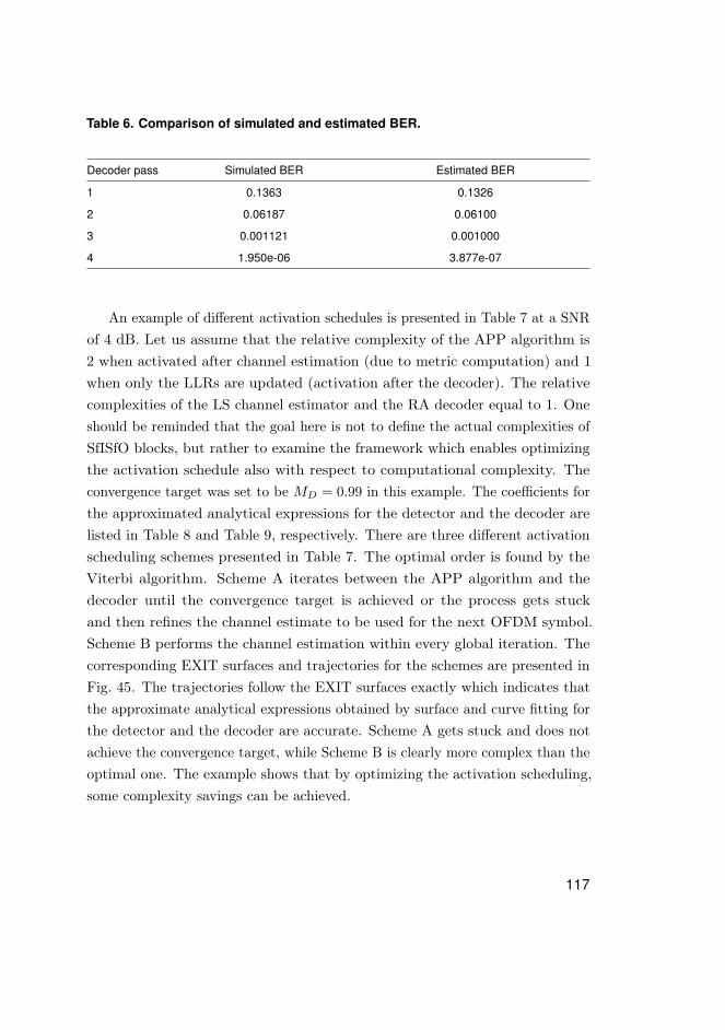
Table 6. Comparison of simulated and estimated BER.

Decoder pass Simulated BER Estimated BER

1 0.1363 0.1326

2 0.06187 0.06100

3 0.001121 0.001000

4 1.950e-06 3.877e-07

An example of different activation schedules is presented in Table 7 at a SNRof 4 dB. Let us assume that the relative complexity of the APP algorithm is2 when activated after channel estimation (due to metric computation) and 1when only the LLRs are updated (activation after the decoder). The relativecomplexities of the LS channel estimator and the RA decoder equal to 1. Oneshould be reminded that the goal here is not to define the actual complexities ofSfISfO blocks, but rather to examine the framework which enables optimizingthe activation schedule also with respect to computational complexity. Theconvergence target was set to be MD = 0.99 in this example. The coefficients forthe approximated analytical expressions for the detector and the decoder arelisted in Table 8 and Table 9, respectively. There are three different activationscheduling schemes presented in Table 7. The optimal order is found by theViterbi algorithm. Scheme A iterates between the APP algorithm and thedecoder until the convergence target is achieved or the process gets stuckand then refines the channel estimate to be used for the next OFDM symbol.Scheme B performs the channel estimation within every global iteration. Thecorresponding EXIT surfaces and trajectories for the schemes are presented inFig. 45. The trajectories follow the EXIT surfaces exactly which indicates thatthe approximate analytical expressions obtained by surface and curve fitting forthe detector and the decoder are accurate. Scheme A gets stuck and does notachieve the convergence target, while Scheme B is clearly more complex than theoptimal one. The example shows that by optimizing the activation scheduling,some complexity savings can be achieved.

117

Table 7. Example of different activation orders ([3],published by permission ofIEEE).

Scheme Schedule Complexity

Optimal 1 3 1 3 2 1 3 1 3 2 1 3 15

A 1 3 1 3 1 3 1 3 1 3 1 3 ... –

B 1 3 2 1 3 2 1 3 2 1 3 2 1 3 2 20

Table 8. Coefficients for detector.

a30 a21 a20 a12 a11 a10 a03 a02 a01 a00

0.0026 -0.0107 -0.0296 0.0039 0.1041 0.0931 -0.0216 0.1137 0.0427 0.2102

Table 9. Coefficients for decoder.

a3 a2 a1 a0

-12.3957 12.7838 -1.6198 0.0563

118

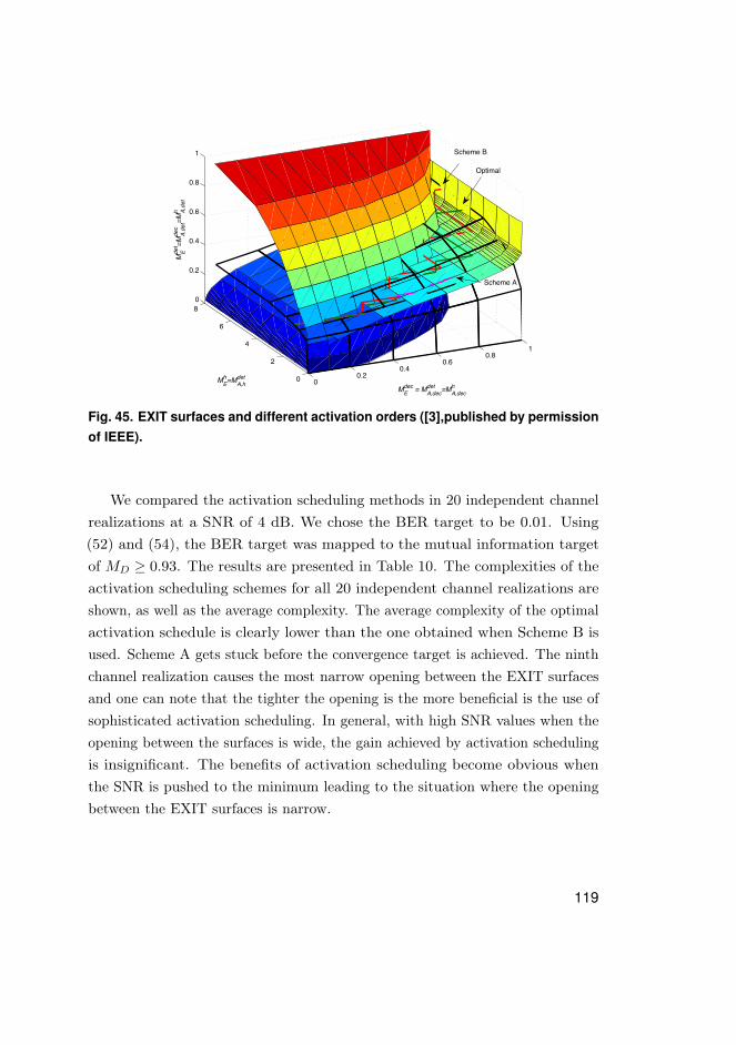
00.2

0.40.6

0.81

0

2

4

6

80

0.2

0.4

0.6

0.8

1

MEdec = MA,dec

det =MA,dech

MEh=MA,h

det

MEde

t =MA,

det

dec

=MA,

det

hOptimal

Scheme B

Scheme A

Fig. 45. EXIT surfaces and different activation orders ([3],published by permissionof IEEE).

We compared the activation scheduling methods in 20 independent channelrealizations at a SNR of 4 dB. We chose the BER target to be 0.01. Using(52) and (54), the BER target was mapped to the mutual information targetof MD ≥ 0.93. The results are presented in Table 10. The complexities of theactivation scheduling schemes for all 20 independent channel realizations areshown, as well as the average complexity. The average complexity of the optimalactivation schedule is clearly lower than the one obtained when Scheme B isused. Scheme A gets stuck before the convergence target is achieved. The ninthchannel realization causes the most narrow opening between the EXIT surfacesand one can note that the tighter the opening is the more beneficial is the use ofsophisticated activation scheduling. In general, with high SNR values when theopening between the surfaces is wide, the gain achieved by activation schedulingis insignificant. The benefits of activation scheduling become obvious whenthe SNR is pushed to the minimum leading to the situation where the openingbetween the EXIT surfaces is narrow.

119

Table 10. Complexity of activation ordering methods in different channel realiza-tions.

Channel Optimal A B

1 13 – 15

2 15 – 19

3 11 – 15

4 15 – 19

5 15 – 19

6 15 – 19

7 19 – 23

8 16 – 19

9 35 – 47

10 17 – 23

11 15 – 19

12 17 – 19

13 11 – 15

14 15 – 19

15 15 – 19

16 15 – 19

17 13 – 19

18 17 – 19

19 15 – 19

20 17 – 23

Average 16.05 – 20.40

complexity


The problem of finding the optimal activation schedule for the detector, thechannel estimator and the decoder in an iterative receiver was considered.The proposed concept was based on EXIT chart analysis and monotonicityof the EXIT functions. A semi-analytical expression was derived for the LS

120

channel estimator and it was shown to closely follow the measured results. TheEXIT functions for the APP algorithm and the RA decoder were obtained bysimulations and approximate analytical expressions were found by using surfaceand curve fitting, respectively. Two trellis based algorithms, the brute-force andViterbi algorithms, were shown to find the optimal activation schedule usingthe EXIT functions. The algorithms are optimal in the sense that they findthe activation schedule which achieves the convergence target with minimalcomplexity. The Viterbi algorithm itself is less complex than the brute-forcealgorithm. The Viterbi algorithm was compared to some conventional activationscheduling methods and the results showed that some gain in complexity andperformance can be achieved by the proposed concept in general. In particular, ifthe SNR is pushed to the minimum and the opening between the EXIT surfacesis narrow, remarkable gain is achieved.

When considering the practicality of the proposed concept, there are two issueswhich are left for future work. The major issue is the well known applicabilitylimitation of EXIT analysis for only relatively long code or symbol block lengths.However, some light is shed on that issue in [180] and [179]. The other issue isthe lack of an analytical solution for the optimal detector EXIT function. Thiscauses difficulties in finding activation schedules in time varying channels. Onepossible solution could be the use of a look-up table from which the appropriateEXIT surface (the coefficients for the 3rd order surface) would be chosen basedon the channel characteristics, e.g., instantaneous SNR and instantaneous rootmean square delay spread.

121

7 Conclusions and future work

The aim of this thesis in a broad sense was to study receiver algorithms whichenable efficient use of radio spectrum. This was motivated by the increasing needsfor wireless data and the demand for lower energy consumption. In particular,the focus was in detection, decoding, and channel estimation. To reach maximalefficiency in spectral use from the algorithm perspective, the use of optimalalgorithms would be the most favorable way. Apparently, the optimal algorithmsfrom a complexity point of view would lead to intractable computationalcomplexities and, thus, approximations of the optimal ones were studied in thisthesis. Chapter 2 contained a literature review of previous and parallel workrelated to channel estimation, detection, and iterative detection, decoding, andchannel estimation in MIMO-OFDM systems. Chapter 3 introduced the signaland channel models for the MIMO-OFDM system. The concept of iterativedetection and decoding was also presented in more detail.

Chapter 4 focused on the MIMO detection part of the iterative receiver.Perfect channel information was assumed to be at the receiver. An iterativereceiver composed of a list detection based soft MIMO detector and a turbodecoder was considered. It was shown that the feedback from the decoder tothe list detector improves the performance or enables using smaller list sizevalues. Further gain was achieved by using a priori information from thedecoder to re-calculate the candidate list during global iterations instead ofonly re-calculating the LLRs. What remains as an open question is whetherthe best way from the complexity point of view to reach a certain performancetarget is to invest in list size, in conventional global iterations, or in globaliterations with list re-calculation. The novel list PIC detector was derived andcompared to the optimal APP algorithm, the K-best LSD, and the IR-LSD. Theresults showed that the list PIC detector offers close to optimal performance withreduced complexity and a performance gain over the K-best LSD with properinitialization. The LMMSE proved out to be good enough in the initializationin a 2× 2 antenna configuration, however, with a 4× 4 antenna configurationwith higher order modulations it was inadequate. The initialization mightbe improved by various techniques (like lattice reduction [107] or semidefinite

123

relaxation based detection [128]), which could be a fruitful research topic. TheIR-LSD offers performance gain over the other studied list detectors. However,in the case of a 2× 2 antenna configuration, the gain over the list PIC detectoris not substantial. The complexity of the list PIC detector is of the same orderas with the K-best LSD and the metric-first search based IR-LSD algorithmwas found to be the least complex in a 2× 2 antenna configuration. However,taking into account that a 2× 2 antenna configuration and LMMSE detectionwill most likely be the first step when employing MIMO processing, the list PICdetector might offer quite an attractive second step due to the straightforwardimplementation.

Chapter 5 considered channel estimation for a MIMO-OFDM system. Decisiondirected (DD) and iterative channel estimation were compared to preamblebased channel estimation in an iterative receiver composed of a soft MIMOdetector, a channel estimator, and the turbo decoder. The conventional LSestimator operating in DD mode requires the inversion of a matrix with the sizeper dimension dependent on the number of transmit antennas and the lengthof the channel impulse response. The matrix inversion can be avoided withthe FD-SAGE channel estimator with constant envelope modulation. However,the drawback with the FD-SAGE channel estimator is the required inversionof a matrix of a size depending on the length of the channel impulse responsewhen non-constant envelope constellations are used. The TD-SAGE estimatorwas derived to lower the complexity by avoiding the matrix inversion withoutperformance degradation.

The performances of the DD SAGE channel estimators were compared tothat of the preamble based LS channel estimator with and without MMSEpost-processing using various preamble densities. According to the results, theuse of DD SAGE channel estimation is beneficial if the channel coding is overone OFDM symbol and with preamble overheads less than 16.7%. Despite thefast fading channel, it was possible to decrease the preamble overhead from 17%to 4% losing only 0.2 dB in performance and, with a 0.5 dB loss in performance,overhead under 1% was achievable with DD SAGE channel estimation. TheSAGE estimator performance was further improved by using the MMSE filterand the previous channel estimates to predict the initial guess. The re-estimationof the channel state within the global iterations, i.e., iterative channel estimation,did not give any gain in the studied cases. However, the activation schedule of the

124

channel estimation was not adapted for the instantaneous channel state. Thus,one cannot state that there is no gain to be achieved by using iterative channelestimation with a dynamic activation schedule. The architecture examples werepresented for the preamble based LS estimator and the FD-SAGE estimatorassuming constant envelope constellation. It was also shown that the timecorrelation of the channel can be exploited by MMSE filtering to improve channelestimation performance with only a small increase in complexity by using fewpre-calculated filters.

The list detector study provided in Chapter 4 was extended for the case ofan estimated channel in Chapter 5. The results were well aligned with thoseobtained with ideal channel state information in the receiver. The list PICdetector offers close to optimal performance with reduced complexity and aperformance gain over the K-best LSD with proper initialization. The LMMSEwas shown to be good enough for initialization in the most practical MIMOconfiguration, i.e., a 2× 2 antenna configuration, however, with a t4× 4 antennaconfiguration with higher order modulations it was inadequate. The IR-LSDoffered performance gain over the other studied list detectors. However, in thecase of a 2× 2 antenna configuration the gain over the list PIC detector was notsubstantial.

Chapter 6 presented a framework for the activation scheduling of a soft MIMOdetector, a channel decoder, and a channel estimator. The proposed concept wasbased on EXIT chart analysis. A semi-analytical method was derived for the LSchannel estimator and it was shown to closely follow the simulated results. TheEXIT functions for the APP algorithm and the RA decoder were obtained bysimulations and approximate analytical expressions were found by using surfaceand curve fitting, respectively. Two trellis based algorithms, the brute-force andViterbi algorithms, were shown to find the optimal activation schedule usingthe EXIT functions. The algorithms are optimal in the sense that they findthe activation schedule which achieves the convergence target with minimalcomplexity. The Viterbi algorithm itself is less complex than the brute-forcealgorithm. The Viterbi algorithm was compared to some conventional activationscheduling methods and the results showed that some gain in complexity andperformance can be achieved by the proposed concept in general. In particular, ifthe SNR is pushed to the minimum and the opening between the EXIT surfacesis narrow, remarkable gain is achieved.

125

When considering the practicality of the proposed concept, there are two issueswhich are left for future work. The major issue is the well known applicabilitylimitation of EXIT analysis for only relatively long code or symbol block lengths.However, some light is shed on that issue in [180] and [179]. The other issueis the lack of an analytical solution of the optimal detector EXIT chart. Thiscauses difficulties in finding activation schedules in time varying channels. Onepossible solution could be the use of a look-up table from which the appropriateEXIT surface (the coefficients for the 3rd order surface) would be chosen basedon the channel characteristics, e.g., instantaneous SNR and instantaneous rootmean square delay spread. Another future topic could be to use, for instance,the TD-SAGE channel estimator instead of the LS estimator and to furtheroptimize the channel estimator iterations. The decoder iterations could also beoptimized with the framework to prevent running unnecessary iterations.

Based on the results presented in this thesis, following design recommendationsare drawn. If the conventional preamble/pilot density is used (e.g., as in LTE andWiMAX), the DD channel estimation algorithms presented in the thesis do notbring any benefit. Instead, the preamble based LS with MMSE post-processingshould be used. However, if the reference signal density is significantly decreased,the TD-SAGE channel estimator is recommended out of the studied ones, sinceit allows for the use of non-constant envelope constellation without an increase incomplexity. If detection algorithms with fixed complexity are preferred, the listPIC algorithm should be chosen for detection in a 2× 2 antenna configurationand the K-best LSD in a 4× 4 antenna configuration. If the complexity can varyfrom one channel realization to another, the IR-LSD would be the recommendedone. Depending on the latency limitations, the global iterations should beused, as they provide performance gain. The activation scheduling frameworkpresented in the thesis requires some further study before it can be applied topractical systems. However, the results indicate that the iteration activationsshould be carefully determined.

126

References

1. Ylioinas J & Juntti M (2009) Iterative joint detection, decoding, and channelestimation in turbo coded MIMO-OFDM. IEEE Transactions on VehicularTechnology 58(4): 1784–1796.

2. Ylioinas J, Karjalainen J & Juntti M (2009, submitted) Scheduling of theactivations in iterative detection, decoding, and channel estimation for MIMO-OFDM. IEEE Transactions on Communications .

3. Ylioinas J, Karjalainen J & Juntti M (2010) On the activation ordering of detector,decoder, and channel estimator in iterative receiver for MIMO-OFDM. IEEEInternational Conference on Communications. Cape-Town, South-Africa, 1–6.

4. Ylioinas J, Madanahally R & Juntti M (2009) Avoiding matrix inversion in DDSAGE channel estimation in MIMO-OFDM with M-QAM. IEEE VehicularTechnology Conference. Anchorage, Alaska, 1–5.

5. Ylioinas J & Juntti M (2007) An iterative receiver design using a novel SAGEbased list detector in turbo coded OFDM. IEEE Vehicular Technology Conference.Dublin, Ireland, 1971–1975.

6. Ylioinas J & Juntti M (2007) An iterative receiver for joint detection, decoding,and channel estimation in turbo coded MIMO OFDM. Asilomar Conference onSignals, Systems and Computers. Pacific Grove, CA, 1784–1796.

7. Ylioinas J & Juntti M (2008) Comparison of three list detectors in iterativedecoding and channel estimation in MIMO OFDM. IEEE International Symposiumon Spread Spectrum Techniques and Applications. Bologna, Italy, 1581–1585.

8. Ylioinas J, Tiiro S & Juntti M (2009) Improving channel estimation with turbofeedback and time domain filtering in MIMO-OFDM. ITG Workshop on SmartAntennas. Berlin, Germany, 275–280.

9. Tiiro S, Ylioinas J, Myllyla M & Juntti M (2009) Implementation of the leastsquares channel estimation algorithm for MIMO- OFDM systems. ITG Workshopon Smart Antennas. Berlin, Germany, 155–161.

10. Ylioinas J & Juntti M (2006) EM based iterative receiver for joint decoding andchannel parameter estimation in space-frequency turbo coded OFDM. IEEEInternational Symposium on Personal, Indoor and Mobile Radio Communications.Helsinki, Finland, 1–5.

11. Ylioinas J & Juntti M (2005) EM based joint data decoding and channel estimationin space-frequency turbo coded OFDM. International Symposium on WirelessPersonal Multimedia Communications. Aalborg, Denmark, 1–5.

12. Ylioinas J, Hooli K, Kiiskilä K & Juntti M (2005) Interference suppression inMIMO communication for WCDMA downlink. IEEE Vehicular TechnologyConference. Stockholm, Sweden, vol. 2, 831–835.

13. Ylioinas J, Hooli K, Kiiskilä K & Juntti M (2004) Interference suppression inMIMO HSDPAcommunication. Proceedings of the Nordic Signal ProcessingSymposium. Espoo, Finland, 228–231.

14. Juntti MJ, Hooli K, Kiiskilä K & Ylioinas J (2007) Space-time equalizers for MIMOhigh speed WCDMA downlinks. IEEE Transactions on Wireless Communications

127

6(7): 2582–2592.15. Kiiskilä K, Hooli K, Ylioinas J & Juntti M (2005) Interference resistant receivers

for WCDMA MIMO downlink. IEEE Vehicular Technology Conference. Stockholm,Sweden, 836–840.

16. Kiiskilä K, Hooli K, Ylioinas J & Juntti M (2004) Interference resistant receiversfor MIMO HSDPA. Proceedings of the Nordic Signal Processing Symposiumincluding the Finnish Wireless Communications Workshop. Oulu, Finland, 1–5.

17. Goldsmith A (2005) Wireless Communications. Cambridge University Press, NewYork, USA.

18. Molisch AF (2005) Wireless Communications. John Wiley & Sons, Chichester,England.

19. De Vriendt J, Laine P, Lerouge C & Xu X (2002) Mobile network evolution: arevolution on the move. IEEE Communications Magazine 40(4): 104–111.

20. Tse D & Viswanath P (2005) Fundamentals of Wireless Communication. CambridgeUniversity Press, Cambridge, UK.

21. Holma H & Toskala A (2000) WCDMA for UMTS Radio Access for ThirdGeneration Mobile Communications. John Wiley & Sons, first edition.

22. Holma H & Toskala A (2006) HSDPA/HSUPA for UMTS: High Speed RadioAccess for Mobile Communications. John Wiley & Sons, first edition.

23. Astely D, Dahlman E, Furuskar A, Jading Y, Lindstrom M & Parkvall S (2009)LTE: the evolution of mobile broadband - [LTE part ii: 3GPP release 8]. IEEECommunications Magazine 47(4): 44–51.

24. Ekstrom H, Furuskar A, Karlsson J, Meyer M, Parkvall S, Torsner J & Wahlqvist M(2006) Technical solutions for the 3G Long-Term Evolution. IEEE CommunicationsMagazine 44(3): 38–45.

25. ANSI/IEEE Standard 80211,1999 Edition (R2003) (2003). Information technology- telecommunications and information exchange between systems - local andmetropolitan area networks - specific requirements part 11: Wireless LAN mediumaccess control (MAC) and physical layer (PHY) specifications.

26. IEEE Standard 80216 (2004). IEEE standard for local and metropolitan areanetworks part 16: Air interface for fixed broadband wireless access systems.

27. IEEE Standard 80216eD6 (2004). IEEE standard for local and metropolitanarea networks part 16: Air interface for fixed broadband wireless access systems:Amendment for physical and medium access control layers for combined fixed andmobile operation in licenced bands.

28. 3rd Generation Partnership Project (3GPP); Technical Specification GroupRadio Access Network (2009) Requirements for further advancements for evolveduniversal terrestrial radio access (e-utra) (lte-advanced) (release 8). Technicalreport, 3rd Generation Partnership Project (3GPP).

29. Proakis JG (2000) Digital Communications. McGraw-Hill, New York, 4th edition.30. Chang RW (1966) Synthesis of band-limited orthogonal signals for multichannel

data transmission. Bell Systems Technical Journal 45: 1775–1796.31. Weinstein SB & Ebert PM (1971) Data transmission by frequency division

multiplexing using the discrete Fourier transform. IEEE Transactions on Commu-nication Technology 19(5): 628–634.

128

32. Cimini LJ (1985) Analysis and simulation of a digital mobile channel usingorthogonal frequency division multiplexing. IEEE Transactions on Communications33(7): 665–675.

33. Sklar B (1997) Rayleigh fading channels in mobile digital communication systemspart I: Characterization. IEEE Communications Magazine 35(7): 90–100.

34. Hata M (1980) Empirical formula for propagation loss in land mobile radioservices. IEEE Transactions on Vehicular Technology 29(3): 317–325.

35. Redl S, Weber M & Oliphant M (1998) GSM and Personal CommunicationsHandbook. Artech House mobile communications library.

36. Bingham JAC (1990) Multicarrier modulation for data transmission: an ideawhose time has come. IEEE Communications Magazine 28(5): 5–14. TelebitCorporation, USA.

37. Wang Z & Giannakis GB (2000) Wireless multicarrier communications. IEEESignal Processing Magazine 17(3): 29–48.

38. Cover TM & Thomas JA (1991) Elements of Information Theory. John Wiley,New York, USA.

39. Shannon CE (1948) A mathematical theory of communications. The Bell SystemTechnical Journal 27: 379–423, 623–656.

40. Hwang T, Yang C, Wu G, Li S & Li G (2009) Ofdm and its wireless applications:A survey. IEEE Transactions on Vehicular Technology 58(4): 1673–1694.

41. Gesbert D, Shafi M, Shiu D, Smith PJ & Naguib A (2003) From theory topractice: An overview of MIMO space-time coded wireless systems. IEEE Journalon Selected Areas in Communications 21(3): 281–302.

42. Paulraj AJ, Gore DA, Nabar RU & Bolcskei H (2004) An overview of MIMOcommunications — A key to gigabit wireless. Proceedings of the IEEE 92(2):198–218.

43. Paulraj AJ, Nabar RU & Gore DA (2003) Introduction to Space-Time WirelessCommunications. Cambridge University Press, Cambridge, UK.

44. Boelcskei H, Gesbert D, Papadias CB & van der Veen AJ (2006) Space-TimeWireless Systems: From Array Processing to MIMO Communications. CambridgeUniversity Press, Cambridge, UK.

45. Foschini GJ & Gans MJ (1998) On limits of wireless communications in a fadingenvironment when using multiple antennas. Wireless Personal Communications,Kluwer Academic Publishers 6: 311–335.

46. Telatar IE (1995) Capacity of multi-antenna Gaussian channels. Technical report,Bell Laboratories. Internal Tech.Memo, pp. 1–28.

47. Winters J (1987) On the capacity of radio communication systems with diversity ina Rayleigh fading environment. IEEE Journal on Selected Areas in Communications5(5): 871–878.

48. Foschini G (1996) Layered space–time architecture for wireless communication ina fading environment when using multi-element antennas. Bell Labs TechnicalJournal 1(2): 41–59.

49. Foschini GJ, Golden GD, Valenzuela RA & Wolniansky PW (1999) Simplifiedprocessing for high spectral efficiency wireless communication employing multi-element arrays. IEEE Journal on Selected Areas in Communications 17(11):1841–1852.

129

50. Golden GD, Foschini CJ, Valenzuela RA & Wolniansky PW (1999) Detectionalgorithm and initial laboratory results using V-BLAST space-time communicationarchitecture. Electronics Letters 35(1): 14–16.

51. Tarokh V, Seshadri N & Calderbank AR (1998) Space-time codes for high datarate wireless communication: Performance criterion and code construction. IEEETransactions on Information Theory 44(2): 744–765.

52. Alamouti S (1998) A simple transmit diversity technique for wireless communica-tions. IEEE Journal on Selected Areas in Communications 16(8): 1451–1458.

53. Tarokh V, Jafarkhani H & Calderbank AR (1999) Space-time block codes fromorthogonal designs. IEEE Transactions on Information Theory 45(5): 1456–1467.

54. Zheng L & Tse DNC (2003) Diversity and multiplexing: A fundamental tradeoffin multiple-antenna channels. IEEE Transactions on Information Theory 49(5):1073–1096.

55. Heath J RW & Love D (2005) Multimode antenna selection for spatial multiplexingsystems with linear receivers. IEEE Transactions on Signal Processing 53(8):3042–3056.

56. Raleigh GG & Cioffi JM (1998) Spatio-temporal coding for wireless communication.IEEE Transactions on Communications 46(3): 357–366.

57. Boelcskei H, Gesbert D & Paulraj AJ (2002) On the capacity of OFDM-basedspatial multiplexing systems. IEEE Transactions on Communications 50(2):225–234.

58. Sampath H, Talwar S, Tellado J, Erceg V & Paulraj A (2002) A fourth-generationMIMO-OFDM broadband wireless system: design, performance, and field trialresults. IEEE Communications Magazine 40(9): 143–149.

59. Boelcskei H (2006) MIMO-OFDM wireless systems: Basics, perspectives, andchallenges. IEEE Transactions on Communications 13(4): 31–37.

60. 3rd Generation Partnership Project (3GPP) (2006) Physical layer aspect forevolved universal terrestrial radio access (UTRA). Technical report, 3rd GenerationPartnership Project (3GPP).

61. 3rd Generation Partnership Project (3GPP); Technical Specification Group RadioAccess Network (2009) Further advancements for e-utra physical layer aspects(release 9). Technical report, 3rd Generation Partnership Project (3GPP).

62. (ITU) ITU (2008) ICTs and climate change: ITU background report. ITU/MICJapan Symposium on ICTs and Climate Change. Kyoto, Japan, 1–25.

63. Meyr H, Moeneclaey M & Fechtel SA (1998) Digital Communication Receivers:Synchronization, Channel Estimation and Signal Processing. John Wiley andSons, New York, USA.

64. Himsoon T, Su W & Liu K (2006) Single-block differential transmit schemefor broadband wireless MIMO-OFDM systems. IEEE Transactions on SignalProcessing 54(9): 3305–3314.

65. Cano A, M X & Giannakis G (2005) Block-differential modulation over doublyselective wireless fading channels. IEEE Transactions on Communications 53(12):2157–2166.

66. El-Arabawy A & Gupta S (1997) Reduced mobile complexity scheme for fastfading channel estimation in OFDM-FDD mobile communication systems. IEEE6th International Conference on Universal Personal Communications. San Diego,

130

CA, 274–278.67. Lohan ES (2003) Multipath delay estimators for fading channels with applications

in CDMA receivers and mobile positioning. Ph.D. thesis, Tampere University ofTechnology, Finland.

68. Shin C, Heath R & Powers E (2007) Blind channel estimation for MIMO-OFDMsystems. IEEE Transactions on Vehicular Technology 56(2): 670–685.

69. Ozdemir M & Arslan H (2007) Channel estimation for wireless OFDM systems.IEEE Communications Surveys & Tutorials 9(2): 18–48.

70. Leus G & van der Veen A (2005) Channel estimation in: Kaiser T. et al., eds,Smart Antenna: State of Art. Hindavi Publishing Corporation.

71. Cavers JK (1991) An analysis of pilot symbol assisted modulation for Rayleighfading channels. IEEE Transactions on Vehicular Technology 40(4): 686–693.

72. Morelli M & Mengali U (2001) A comparison of pilot-aided channel estimationmethods for OFDM systems. IEEE Transactions on Signal Processing 49(12):3065–3073.

73. Li Y (2000) Pilot-symbol-aided channel estimation for OFDM in wireless systems.IEEE Transactions on Vehicular Technology 49(4): 1207–1215.

74. Tong L, Sadler B & Dong M (2004) Pilot-assisted wireless transmissions: generalmodel, design criteria, and signal processing. IEEE Signal Processing Magazine21(6): 12–25.

75. Barhumi I, Leus G & Moonen M (2003) Optimal training design for MIMO OFDMsystems in mobile wireless channels. IEEE Transactions on Signal Processing51(6): 1615–1624.

76. Negi R & Cioffi J (1998) Pilot tone selection for channel estimation in a mobileOFDM system. IEEE Transactions on Consumer Electronics 44(3): 1122–1128.

77. Li Y (2002) Simplified channel estimation for OFDM systems with multipletransmit antennas. IEEE Transactions on Wireless Communications 1(1): 67–75.

78. Dong M & Tong L (2002) Optimal design and placement of pilot symbols forchannel estimation. IEEE Transactions on Signal Processing 50(12): 3055–3069.

79. Adireddy S, Lang T & Viswanathan H (2002) Optimal placement of training forfrequency-selective block-fading channels. IEEE Transactions on InformationTheory 48(8): 2338–2353.

80. Ohno S & Giannakis G (2004) Capacity maximizing MMSE-optimal pilots forwireless OFDM over frequency-selective block Rayleigh-fading channels. IEEETransactions on Information Theory 50(9): 2138–2145.

81. Ma X, Giannakis G & Ohno S (2003) Optimal training for block transmissionsover doubly selective wireless fading channels. IEEE Transactions on SignalProcessing 51(5): 1351–1366.

82. Cai X & Giannakis G (2004) Error probability minimizing pilots for OFDMwith M-PSK modulation over rayleigh-fading channels. IEEE Transactions onVehicular Technology 53(1): 146–155.

83. Kay SM (1993) Fundamentals of Statistical Signal Processing: Estimation Theory.Prentice-Hall, Englewood Cliffs, NJ, USA.

84. Chang MX & Su Y (2002) Model-based channel estimation for OFDM signals inRayleigh fading. IEEE Transactions on Communications 50(4): 540–544.

131

85. Rinne J & Renfors M (1996) Pilot spacing in orthogonal frequency divisionmultiplexing systems on practical channels. IEEE Transactions on ConsumerElectronics 42(4): 959–962.

86. Kang SG, Ha YM & Joo EK (2003) A comparative investigation on channelestimation algorithms for ofdm in mobile communications. IEEE Transactions onBroadcasting 49(2): 142–149.

87. Coleri S, Ergen M, Puri A & Bahai A (2002) Channel estimation techniques basedon pilot arrangement in OFDM systems. IEEE Transactions on Broadcasting48(3): 223–229.

88. Zhang H & Li Y (2004) Clustered OFDM with adaptive antenna arrays forinterference suppression. IEEE Transactions on Wireless Communications 3(6):2189–2197.

89. Edfors O, Sandell M, van de Beek JJ, Wilson S & Börjesson P (1998) OFDMchannel estimation by singular value decomposition. IEEE Transactions onCommunications 46(7): 931–939.

90. Li Y, Cimini LJ & Sollenberger NR (1998) Robust channel estimation forOFDM systems with rapid dispersive fading channels. IEEE Transactions onCommunications 46(7): 902–915.

91. Miao H & Juntti M (2005) Space-time channel estimation and performanceanalysis for wireless MIMO-OFDM systems with spatial correlation. IEEETransactions on Vehicular Technology 54(6): 2003 – 2016.

92. Miao H (2007) Channel estimation and positioning for multiple antenna systems.Ph.D. thesis, Department of Electrical and Information Engineering, University ofOulu, Oulu, Finland.

93. Bulumulla S, Kassam S & Venkatesh S (2000) A systematic approach to detectingOFDM signals in a fading channel. IEEE Transactions on Communications 48(5):725–728.

94. Al-Naffouri T, Bahai A & Paulraj A (2002) An EM-based OFDM receiver fortime-variant channels. IEEE Global Telecommunication Conference. Taipei,Taiwan, vol. 1, 589–593.

95. Chini A, W Y, El-Tanany M & Mahmoud S (1998) Filtered decision feedbackchannel estimation for ofdm-based dtv terrestrial broadcasting system. IEEETransactions on Broadcasting 44(1): 2–11.

96. Li Y, Seshadri N & Ariyavisitakul S (1999) Channel estimation for OFDM systemswith transmitter diversity in mobile wireless channels. IEEE Journal on SelectedAreas in Communications 17(3): 461–471.

97. Li Y, Winters JH & Sollenberger NR (2002) MIMO-OFDM for wireless communi-cations: Signal detection with enhanced channel estimation. IEEE Transactionson Communications 50(9): 1471–1477.

98. Sari H, Karam G & Jeanclaud I (1994) Frequency-domain equalization of mobileradio and terrestrial broadcast channels. IEEE Global TelecommunicationConference. San Francisco, CA, 1–5.

99. Lupas R & Verdú S (1989) Linear multiuser detectors for synchronous code-division multiple-access channels. IEEE Transactions on Information Theory34(1): 123–136.

132

100. Xie Z, Short RT & Rushforth CK (1990) A family of suboptimum detectorsfor coherent multiuser communications. IEEE Journal on Selected Areas inCommunications 8(4): 683–690.

101. Artes H, Seethaler D & Hlawarsch F (2003) Efficient detection algorithms forMIMO channels: A geometrical approach to approximate ML detection. IEEETransactions on Signal Processing 51(11): 2808–2820.

102. Winters JH, Salz J & Gitlin RD (1994) The impact of antenna diversity on the ca-pacity of wireless communication systems. IEEE Transactions on Communications42(2/3/4).

103. Gore D, Heath J RW & Paulraj A (2002) On performance of the zero forcingreceiver in presence of transmit correlation. IEEE International Symposium onInformation Theory. 159.

104. Wolniansky PW, Foschini GJ, Golden GD & Valenzuela RA (1998) V-BLAST:An architecture for realizing very high data rates over the rich-scattering wirelesschannel. International Symposium on Signals, Systems, and Electronics. Pisa,Italy, 295–300.

105. Yao H & Wornell G (2002) Lattice-reduction-aided detectors for MIMO communi-cation systems. IEEE Global Telecommunication Conference. Taipei, Taiwan,vol. 1, 424–428.

106. Windpassinger C & Fischer RFH (2003) Low-complexity near-maximum-likelihooddetection and precoding for MIMO systems with lattice reduction. Proceedings ofthe IEEE Information Theory Workshop. Paris, France, 345–348.

107. Wübben D, Böhnke R, Kühn V & Kammeyer K (2004) Near-maximum-likelihooddetection of MIMO systems using MMSE-based lattice-reduction. IEEE Interna-tional Conference on Communications. Paris, France, vol. 2, 798–802.

108. Wubben D, Bohnke R, Kuhn V & Kammeyer KD (2004) MMSE-based lattice-reduction for near-ML detection of MIMO systems. ITG Workshop on SmartAntennas. Munich, Germany, 106–113.

109. Fincke U & Pohst M (1985) Improved methods for calculating vectors of shortlength in a lattice, including a complexity analysis. Mathematics of Computation44(5): 463–471.

110. Damen MO, Chkeif A & Belfiore JC (2000) Lattice code decoder for space-timecodes. IEEE Communications Letters 4(5): 161–163.

111. Damen MO, Gamal HE & Caire G (2003) On maximum–likelihood detection andthe search for the closest lattice point. IEEE Transactions on Information Theory49(10): 2389–2402.

112. Viterbo E & Bouros J (1999) A universal lattice code decoder for fading channels.IEEE Transactions on Information Theory 45(5): 1639–1642.

113. Murugan A, El Gamal H, Damen M & Caire G (2006) A unified framework fortree search decoding: rediscovering the sequential decoder. IEEE Transactions onInformation Theory 52(3): 933–953.

114. Gowaikar R & Hassibi B (2003) Efficient statistical pruning for maximumlikelihood decoding. IEEE International Conference on Acoustics, Speech, andSignal Processing. Hong Kong, vol. 5, 49–52.

115. Wong K, Tsui C, Cheng RK & Mow W (2002) A VLSI architecture of a K-best lattice decoding algorithm for MIMO channels. Proceedings of the IEEE

133

International Symposium on Circuits and Systems. Scottsdale, AZ, vol. 3, 273–276.116. Guo Z & Nilsson P (2006) Algorithm and implementation of the K-best sphere

decoding for MIMO detection. IEEE Journal on Selected Areas in Communications24(3): 491–503.

117. Jelinek F & Anderson J (1971) Instrumentable tree encoding of informationsources (corresp.). IEEE Transactions on Information Theory 17(1): 118–119.

118. Anderson J & Mohan S (1984) Source and channel coding: An algorithmicapproach. IEEE Transactions on Communications 32(2): 169–176.

119. Schnorr CP & Euchner M (1994) Lattice basis reduction: Improved practicalalgorithms and solving subset sum problems. Mathematical Programming 66(2):181–191.

120. Xu W, Wang Y, Zhou Z & Wang J (2004) A computationally efficient exact MLsphere decoder. IEEE Global Telecommunication Conference. vol. 4, 2594–2598.

121. Zhao W & GB G (2005) Sphere decoding algorithms with improved radius search.IEEE Transactions on Communications 53(7): 1104–1109.

122. Jaldén J & Ottersten B (2005) On the complexity of sphere decoding in digitalcommunications. IEEE Transactions on Signal Processing 53(4): 1474–1484.

123. Hassibi B & Vikalo H (2005) On the sphere-decoding algorithm I. expectedcomplexity. IEEE Transactions on Signal Processing 53(8): 2806–2818.

124. Vikalo H & Hassibi B (2005) On the sphere-decoding algorithm II. generalizations,second-order statistics, and applications to communications. IEEE Transactionson Signal Processing 53(8): 2819–2834.

125. Agrell E, Eriksson T, Vardy A & Zeger K (2002) Closest point search in lattices.IEEE Transactions on Information Theory 48(8): 2201–2214.

126. Ma WK, Davidson T, Wong KM, Luo ZQ & Ching PC (2002) Quasi-maximum-likelihood multiuser detection using semi-definite relaxation with application tosynchronous cdma. IEEE Transactions on Signal Processing 50(4): 912–922.

127. Tan PH & Rasmussen L (2001) The application of semidefinite programming fordetection in CDMA. IEEE Journal on Selected Areas in Communications 19(8):1442–1449.

128. Wiesel A, Eldar YC & Shamai S (2005) Semidefinite relaxation for detection of16-QAM signaling in MIMO channels. IEEE Signal Processing Letters 12(9):653–656.

129. Sidiropoulos N & Luo ZQ (2006) A semidefinite relaxation approach to MIMOdetection for high-order QAM constellations. IEEE Signal Processing Letters13(9): 525–528.

130. Mobasher A, Taherzadeh M, Sotirov R & Khandani A (2007) A near-maximum-likelihood decoding algorithm for MIMO systems based on semi-definite program-ming. IEEE Transactions on Information Theory 53(11): 3869–3886.

131. Jaldén J & Ottersten B (2008) The diversity order of the semidefinite relaxationdetector. IEEE Transactions on Information Theory 54(4): 1406–1422.

132. Berrou C, Glavieux A & Thitimajshima P (1993) Near Shannon limit errorcorrecting coding and decoding: Turbo codes. IEEE International Conference onCommunications. Geneva, Switzerland, vol. 2, 1064–1070.

133. Lodge J, Young R, Hoeher P & Hagenauer J (1993) Separable MAP “filters” forthe decoding of product and concatenated codes. IEEE International Conference

134

on Communications. vol. 3, 1740–1745.134. Douillard C, Jezequel CM, Berrou C, Picart A, Didier P & Glavieux A (1995)

Iterative correction of intersymbol interference: Turbo-equalisation. EuropeanTransactions on Telecommunications 6(5): 507–511.

135. Anastasopoulos A & Chugg KM (1998) Iterative equalization/decoding of TCMfor frequency-selective fading channels. Asilomar Conference on Signals, Systemsand Computers. Pacific Grove, CA, 177–181.

136. Reed MC (1999) Iterative Receiver Techniques for Coded Multiple AccessCommunication Systems. Ph.D. thesis, The University of South Australia,Australia.

137. Hagenauer J, Offer E & Papke L (1996) Iterative decoding of binary block andconvolutional codes. IEEE Transactions on Information Theory 42(2): 429–445.

138. Bahl LR, Cocke J, Jelinek F & Raviv J (1974) Optimal decoding of linear codesfor minimizing symbol error rate. IEEE Transactions on Information Theory20(2): 284–287.

139. Robertson P, Villebrun E & Hoeher P (1995) A comparison of optimal andsub-optimal MAP decoding algorithms operating in the log domain. IEEEInternational Conference on Communications : 1009–1013.

140. Tuchler M, Koetter R & Singer A (2002) Turbo equalization: principles and newresults. IEEE Transactions on Communications 50(5): 754–767.

141. Tuchler M, Singer A & Koetter R (2002) Minimum mean squared error equalizationusing a priori information. IEEE Transactions on Signal Processing 50(3): 673–683.

142. Ariyavisitakul SL (2000) Turbo space-time processing to improve wireless channelcapacity. IEEE Transactions on Communications 48(8): 1347–1359.

143. Stefanov A & Duman T (2001) Turbo-coded modulation for systems with transmitand receive antenna diversity over block fading channels: System model, decodingapproaches, and practical considerations. IEEE Journal on Selected Areas inCommunications 19(5): 958–968.

144. Hochwald B & ten Brink S (2003) Achieving near-capacity on a multiple-antennachannel. IEEE Transactions on Communications 51(3): 389–399.

145. Myllylä M, Juntti M & Cavallaro J (2008) Implementation and complexity analysisof list sphere detector for MIMO-OFDM systems. Asilomar Conference on Signals,Systems and Computers. Pacific Grove, CA, 1852–1856.

146. Myllylä M, Juntti M & Cavallaro J (2009) Architecture design and implementationof the increasing radius - list sphere detector algorithm. IEEE InternationalConference on Acoustics, Speech, and Signal Processing. Taipei, Taiwan, 553–556.

147. Kerttula J, Myllylä M & Juntti M (2007) Implementation of a K-best basedMIMO-OFDM detector algorithm. European Signal Processing Conference.Poznań, Poland, 2149–2153.

148. Xie Y, Li Q & Georghiades C (2007) On some near optimal low complexity detectorsfor MIMO fading channels. IEEE Transactions on Wireless Communications 6(4):1182–1186.

149. Fessler J & Hero A (1994) Space-alternating generalized expectation-maximizationalgorithm. IEEE Transactions on Signal Processing 42(10): 2664–2677.

135

150. Dempster AP, Laird NM & Rubin DB (1977) Maximum likelihood from incompletedata via the EM algorithm. Journal of Royal Statistical Society 39(1): 1–38.

151. McLachlan GJ & Krishnan T (1997) The EM Algorithm and Extensions. Wiley,New York, USA.

152. Otnes R & Tüchler M (2004) Iterative channel estimation for turbo equalizationof time-varying frequency-selective channels. IEEE Transactions on WirelessCommunications 3: 1918–1923.

153. Otnes R & Tüchler M (2002) Soft iterative channel estimation for turbo equal-ization: Comparison of channel estimation algorithms. IEEE InternationalConference on Communication Systems. Singapore, 72–76.

154. Song S, Singer A & Sung KM (2004) Soft input channel estimation for turboequalization. IEEE Transactions on Signal Processing 52(10): 2885–2894.

155. Zhao M, Shi Z & Reed M (2008) Iterative turbo channel estimation for OFDMsystem over rapid dispersive fading channel. IEEE Transactions on WirelessCommunications 7(8): 3174–3184.

156. Georghiades C & Han J (1997) Sequence estimation in the presence of randomparameters via the EM algorithm. IEEE Transactions on Communications 45(3):300–308.

157. Kaleh G (1994) Joint parameter estimation and symbol detection for linear andnonlinear unknown channels. IEEE Transactions on Communications 42(7):2406–2413.

158. Cozzo C & Hughes BL (2003) Joint channel estimation and data detectionin space-time communications. IEEE Transactions on Communications 51(8):1266–1270.

159. Khalighi M & Boutros J (2006) Semi-blind channel estimation using the EMalgorithm in iterative MIMO APP detectors. IEEE Transactions on WirelessCommunications 5(11): 3165–3173.

160. Choi J (2006) MIMO-BICM iterative receiver with the EM based channel estima-tion and simplified MMSE combining with soft cancellation. IEEE Transactionson Signal Processing 54(8): 3247–3251.

161. Wautelet X, Herzet C, Dejonghe A, Louveaux J & Vandendorpe L (2007)Comparison of EM-based algorithms for MIMO channel estimation. IEEETransactions on Communications 55(1): 216–226.

162. Khalighi MA & Bourennane S (2008) Semiblind single-carrier MIMO channelestimation using overlay pilots. IEEE Transactions on Vehicular Technology57(3): 1951–1956.

163. Zheng J & Rao B (2006) LDPC-coded MIMO systems with unknown block fadingchannels: soft MIMO detector design, channel estimation, and code optimization.IEEE Transactions on Signal Processing 54(4): 1504–1518.

164. Lu B, Wang X & Li YG (2002) Iterative receivers for space-time block codedOFDM systems in dispersive fading channels. IEEE Wireless CommunicationsMagazine 1(2): 213–225.

165. Xie Y & Georghiades CN (2003) Two EM–type channel estimation algorithms forOFDM with transmitter diversity. IEEE Transactions on Communications 51(1):106–115.

136

166. Kocian A, Land I & Fleury B (2007) Joint channel estimation, partial successiveinterference cancellation, and data decoding for DS-CDMA based on the SAGEalgorithm. IEEE Transactions on Communications 55(6): 1231–1241.

167. Kocian A & Fleury B (2003) EM-based joint data detection and channel estimationof DS-CDMA signals. IEEE Transactions on Communications 51(10): 1709–1720.

168. Pun MO, Morelli M & Kuo CCJ (2007) Iterative detection and frequencysynchronization for OFDMA uplink transmissions. IEEE Transactions on WirelessCommunications 6(2): 629–639.

169. Fu X, Minn H & Cantrell C (2008) Two novel iterative joint frequency-offsetand channel estimation methods for OFDMA uplink. IEEE Transactions onCommunications 56(3): 474–484.

170. Saemi A, Cances JP & Meghdadi V (2007) Synchronization algorithms forMIMO OFDMA systems. IEEE Transactions on Wireless Communications 6(12):4441–4451.

171. Sun Y, Xiong Z & Wang X (2005) EM-based iterative receiver design withcarrier-frequency offset estimation for MIMO OFDM systems. IEEE Transactionson Communications 53(4): 581–586.

172. Pham TH, Nallanathan A & Liang YC (2008) Joint channel and frequency offsetestimation in distributed MIMO flat-fading channels. IEEE Transactions onWireless Communications 7(2): 648–656.

173. Guenach M, Marey M, Wymeersch H, Steendam H & Moeneclaey M (2008)Turbo estimation and equalization for asynchronous uplink MC-CDMA. IEEETransactions on Wireless Communications 7(4): 1217–1226.

174. ten Brink S (2001) Convergence behavior of iteratively decoded parallel concate-nated codes. IEEE Transactions on Communications 49(6): 1727–1737.

175. Ashikhmin A, Kramer G & ten Brink S (2004) Extrinsic information transfer func-tions: model and erasure channel properties. IEEE Transactions on InformationTheory, 50(11): 2657–2673.

176. ten Brink S (2000) Rate one-half code for approaching the Shannon limit by 0.1dB. Electronics Letters 36(15): 1293–1294.

177. ten Brink S, Kramer G & Ashikhmin A (2004) Design of low-density parity-checkcodes for modulation and detection. IEEE Transactions on Communications52(4): 670–678.

178. ten Brink S & Kramer G (2003) Design of repeat-accumulate codes for iterativedetection and decoding. IEEE Transactions on Signal Processing 51(11): 2764–2772.

179. Li K & Wang X (2005) EXIT chart analysis of turbo multiuser detection. IEEETransactions on Wireless Communications 1(1): 300–311.

180. Lee JW & Blahut RE (2007) Converge analysis and BER performance of finite-length turbo codes. IEEE Transactions on Communications 55(5): 1033–1043.

181. Tuchler M (2002) Convergence prediction for iterative decoding of threefoldconcatenated systems. IEEE Global Telecommunication Conference. Taipei,Taiwan, vol. 2, 1358–1362.

182. Brännström F, Rasmussen LK & Grant AJ (2005) Convergence analysis andoptimal scheduling for multiple concatenated codes. IEEE Transactions onInformation Theory 51(9): 3354–3364.

137

183. Shepherd D, Brannstrom F, Schreckenbach F, Shi Z & Reed M (2008) Adaptiveoptimization of an iterative multiuser detector for turbo-coded CDMA. IEEETransactions on Wireless Communications 7(1): 4284–4293.

184. Huang Y & Ritcey JA (2005) Joint iterative channel estimation and decodingfor bit-interleaved coded modulation over correlated fading channels. IEEETransactions on Wireless Communications 4(5): 2549–2558.

185. Dangl M, Sgraja C & Lindner J (2007) An improved block equalization scheme foruncertain channel estimation. IEEE Transactions on Wireless Communications6(1): 146–156.

186. Otnes R & Tüchler M (2002) EXIT chart analysis applied to adaptive turboequalization. Proceedings of the Nordic Signal Processing Symposium. Hurtigruten,Norway, 1–5.

187. Dangl M, Sgraja C, W T, J L & J E (2003) Joint iterative equalization,demappingand decoding with a soft interference canceller. International Symposium onCommunication Theory and Application. Ambleside, England, 1–5.

188. Shepherd D, Shi Z, Anderson M & Reed M (2007) EXIT chart analysis of aniterative receiver with channel estimation. IEEE Global TelecommunicationConference. Washington,DC, USA, 4010–4014.

189. Pedersen KI, Andersen JB, Kermoal JP & Mogensen P (2000) A stohasticmultiple-input-mobile-output radio channel model for evaluation of space-timecoding algorithms. IEEE Vehicular Technology Conference. Boston, USA, 893–897.

190. Kermoal JP, Schumacher L, Pedersen K, Mogensen PE & Frederiksen F (2002)A stochastic MIMO radio channel model with experimental validation. IEEEJournal on Selected Areas in Communications 20(6): 1211–1226.

191. Xie Y, Georghiades CN & Li Q (2004) A novel low complexity detector for MIMOsystem. Asilomar Conference on Signals, Systems and Computers. Pacific Grove,CA, vol. 1, 208 – 212.

192. Myllylä M, Silvola P, Juntti M & Cavallaro JR (2006) Comparison of two novellist sphere detector algorithms for MIMO-OFDM systems. IEEE InternationalSymposium on Personal, Indoor and Mobile Radio Communications. Helsinki,Finland, 12–16.

193. Myllylä M, Juntti M & Cavallaro JR (2007) A list sphere detector based onDijkstra’s algorithm for MIMO-OFDM system. IEEE International Symposiumon Personal, Indoor and Mobile Radio Communications. Athens, Greece, 1–5.

194. Myllylä M, Juntti M & Cavallaro JR (2007) Implementation aspects of list spheredetector algorithms. IEEE Global Telecommunication Conference. Washington,D.C., USA, 3915–3920.

195. Jaldén J, Barbero LG, Ottersten B & Thompson JS (2009) The error probabilityof the fixed-complexity sphere decoder. IEEE Transactions on Signal Processing57(7): 2711–2720.

196. Barbero LG & Thompson JS (2008) Fixing the complexity of the sphere decoder forMIMO detection. IEEE Transactions on Wireless Communications 7: 2131–2142.

197. 3rd Generation Partnership Project (3GPP); Technical Specification Group RadioAccess Network (2006) Multiplexing and channel coding (FDD) (3G TS 25.212version 7.2.0). Technical report, 3rd Generation Partnership Project (3GPP).

138

198. 3rd Generation Partnership Project (3GPP); Technical Specification Group RadioAccess Network (2002) Radio transmission and reception (3G TS 45.005 version5.4.0 (release 5)). Technical report, 3rd Generation Partnership Project (3GPP).

199. Kerttula J, Myllylä M & Juntti M (2007) Word length and architecture design ofa K-best based MIMO-OFDM detector algorithm. IEEE Workshop on SignalProcessing Advances in Wireless Communications. Helsinki, Finland, 1–5.

200. Golub GH & Loan CFV (1996) Matrix Computations, 3rd ed. The Johns HopkinsUniversity Press, Baltimore.

201. Kailath T & Chun J (1994) Generalized displacement structure for block-Toeplitz,Toeplitz-block, and Toeplitz-derived matrices. SIAM Journal on Matrix Analysisand Applications 15(1): 114–128.

202. Tuchler M & Hagenauer J (2002) EXIT charts of irregular codes. Conference onInformation Sciences and Systems. Baltimore, MD, 748–753.

139


Book orders:Granum: Virtual book storehttp://granum.uta.fi/granum/

S E R I E S C T E C H N I C A

342. Boutellier, Jani (2009) Quasi-static scheduling for fine-grained embeddedmultiprocessing

343. Vallius, Tero (2009) An embedded object approach to embedded systemdevelopment

344. Chung, Wan-Young (2009) Ubiquitous healthcare system based on a wirelesssensor network

345. Väisänen, Tero (2009) Sedimentin kemikalointikäsittely. Tutkimus rehevän ja sisä-kuormitteisen järven kunnostusmenetelmän mitoituksesta sekä sen tuloksellisuu-den mittaamisesta

346. Mustonen, Tero (2009) Inkjet printing of carbon nanotubes for electronicapplications

347. Bennis, Mehdi (2009) Spectrum sharing for future mobile cellular systems

348. Leiviskä, Tiina (2009) Coagulation and size fractionation studies on pulp andpaper mill process and wastewater streams

349. Casteleijn, Marinus G. (2009) Towards new enzymes: protein engineering versusBioinformatic studies

350. Haapola, Jussi (2010) Evaluating medium access control protocols for wirelesssensor networks

351. Haverinen, Hanna (2010) Inkjet-printed quantum dot hybrid light-emittingdevices—towards display applications

352. Bykov, Alexander (2010) Experimental investigation and numerical simulation oflaser light propagation in strongly scattering media with structural and dynamicinhomogeneities

353. Kannala, Juho (2010) Models and methods for geometric computer vision

354. Kela, Lari (2010) Attenuating amplitude of pulsating pressure in a low-pressurehydraulic system by an adaptive Helmholtz resonator

355. Ronkainen, Sami (2010) Designing for ultra-mobile interaction. Experiences and amethod

356. Loikkanen, Mikko (2010) Design and compensation of high performance class ABamplifiers

357. Puikko, Janne (2010) An exact management method for demand driven, industrialoperations

C358etukansi.kesken.fm Page 2 Friday, May 14, 2010 1:28 PM

ABCDEFG

UNIVERS ITY OF OULU P.O.B . 7500 F I -90014 UNIVERS ITY OF OULU F INLAND


S E R I E S E D I T O R S

SCIENTIAE RERUM NATURALIUM

HUMANIORA

TECHNICA

MEDICA

SCIENTIAE RERUM SOCIALIUM

SCRIPTA ACADEMICA

OECONOMICA

EDITOR IN CHIEF

PUBLICATIONS EDITOR

Professor Mikko Siponen

University Lecturer Elise Kärkkäinen

Professor Pentti Karjalainen

Professor Helvi Kyngäs

Senior Researcher Eila Estola

Information officer Tiina Pistokoski



Publications Editor Kirsti Nurkkala

ISBN 978-951-42-6219-7 (Paperback)ISBN 978-951-42-6220-3 (PDF)ISSN 0355-3213 (Print)ISSN 1796-2226 (Online)


TECHNICA


TECHNICA

OULU 2010

C 358

Jari Ylioinas


FACULTY OF TECHNOLOGY,DEPARTMENT OF ELECTRICAL AND INFORMATION ENGINEERING,UNIVERSITY OF OULU;CENTRE FOR WIRELESS COMMUNICATIONS,INFOTECH OULUUNIVERSITY OF OULU

C 358

ACTA

Jari YlioinasC358etukansi.kesken.fm Page 1 Friday, May 14, 2010 1:28 PM

iterative detection, decoding, and channel estimation in...

Documents