Iterative Distillation for Better Uncertainty Estimates in Multitask EmotionRecognition

Didan Deng1, Liang Wu2, Bertram E. Shi3Department of Electronic and Computer Engineering,

Hong Kong University of Science and Technology, Kowloon, Hong Kong{ddeng1, lwuat2}@connect.ust.hk eebert@ust.hk3

Abstract

When recognizing emotions, subtle nuances in displaysof emotion generate ambiguity or uncertainty in emotionperception. Emotion uncertainty has been previously in-terpreted as inter-rater disagreement among multiple an-notators. In this paper, we consider a more common andchallenging scenario: modeling emotion uncertainty whenonly single emotion labels are available. From a Bayesianperspective, we propose to use deep ensembles to captureuncertainty for multiple emotion descriptors, i.e., actionunits, discrete expression labels and continuous descrip-tors. We further apply iterative self-distillation. Itera-tive distillation over multiple generations significantly im-proves performance in both emotion recognition and un-certainty estimation. Our method generates single studentmodels that provide accurate estimates of uncertainty forin-domain samples and a student ensemble that can de-tect out-of-domain samples. Our experiments on emotionrecognition and uncertainty estimation using the Aff-wild2dataset demonstrate that our algorithm gives more reliableuncertainty estimates than both Temperature Scaling andMonte Carol Dropout.

1. Introduction

Understanding human affective states is an essential taskfor many interactive systems (e.g., social robots) or datamining systems (e.g., user profiling). However, unlike ob-ject recognition tasks, emotion perception is strongly af-fected by personal bias, cultural backgrounds and contex-tual information (e.g., environment), which increases theuncertainty of emotion perception.

To obtain a gold standard for emotion recognition, itis common to invite a number of annotators and take themost-agreed emotions as hard labels in emotion datasets[27, 33, 38, 36]. In datasets with huge number of samples[29], it is expensive to invite many annotators. Therefore,

0 1Emotion Uncertainty

Arousal: 0.4Valence: 0.5

HappinessAU26: 0AU25: 1AU24: 0AU23: 0AU15: 1AU12: 1AU10: 1

AU7: 1AU6: 1AU4: 0AU2: 0AU1: 0

Facial Image

Figure 1: An example facial image with classifications gen-erated by our model. The classifications are shown in thelabels in the left. The estimated uncertainty is shown in thebar graph in the right. For example, the emotion is clas-sified as ”Happiness”. The estimated valence and arousalscores are 0.5 and 0.4. The presence or absence of each AUis indicated by 1 or 0. The emotion uncertainty is the nor-malized Shannon’s entropy (i.e., divided by its informationlength). Large uncertainty indicates low confidence. For ex-ample, AU15 ”lip corner depressor” is indicated as present,but with high uncertainty (low confidence). It is not presentin the example image.

each sample is often annotated by one expert only. Singleemotion labels cannot capture inter-rater disagreement.

Previous work often related emotion ambiguity (uncer-tainty) with the variability among multiple raters’ annota-tions. For example, Mower et al. [30] characterized ambi-guity using probability distributions assigned to the emo-tion classes. Han et al. [13] defined emotion uncertainty asperception uncertainty (i.e., inter-rater disagreement). Thesolutions cannot be applied to emotion datasets with onlysingle labels.

To address this problem, we adopt the Bayesian view-

3557

point and interpret emotion uncertainty as uncertainty in theposterior distribution over model weights. It is affected bythe nosie, data distribution, and the model we choose. Itdoes not require multiple raters’ annotations, as required bythe perception uncertainty.

In addition, we consider uncertainty simultaneously formultiple types of emotion labels (i.e., facial action units,basic emotions, valence and arousal), whereas past studiesconsidered only single label types. Our intuition is that hu-man affective states are quite complex, and should be de-scribed using a comprehensive set of emotional descriptors.Uncertainty among different emotion labels may be corre-lated. For example, the relationship between valence andarousal may be related to the uncertainty in perceived va-lence [2].

The recently released Aff-wild2 [22, 17] facilitates mul-titask emotion solutions [20, 24, 7]. The Aff-wild2 datasethas three types of emotion labels: facial action units, emo-tion categories, valence and arousal. Past emotion datasets[27, 33, 38, 21] usually have one or two types of emotion la-bels. However, Aff-wild2 dataset only provides single emo-tion labels, not multiple annotators’ labels.

Using data from the Aff-wild2 dataset, we train deep en-sembles with self-distillation algorithm to improve emotionrecognition and uncertainty estimation. The obtained net-works produce both emotions labels and the estimated un-certainty. The uncertainty is measured by Shannon’s en-tropy computed over the probabilistic output. We give anexample in Figure 1, showing the outputs of our modelgiven a facial image input.

Our primary contributions are as follows:

• For better uncertainty estimation performance, wepropose to apply deep ensembles learned by multi-generational self-distillation. The iterative training ofneural networks improves not only uncertainty estima-tion, but also multitask emotion recognition.

• We design Efficient Multitask Emotion Networks(EMENet) for video emotion recognition. The visualmodel (EMENet-V) only has 1.68M parameters. Thevisual-audio (EMENet-VA) model has 1.91M param-eters.

• We show that single models can estimate uncertaintyreliably on in-domain data, and that the ensembles candetect out-of-distribution (OOD) samples.

2. Related Works2.1. Uncertainty in Emotion

In emotion recognition, uncertainty often refers to per-ception uncertainty, in other words, inter-rater disagree-ment, requiring multiple annotators. Han et al. [13] took the

standard deviation of K emotion labels given by K annota-tors as perception uncertainty. Zhang et al. [37] used Kappacoefficient to represent inter-rater agreement level. Uncer-tainty in emotion recognition has also been used to refer tothe uncertainty in probabilistic models. A work in speechemotion recognition used a probabilistic Gaussian MixtureRegression (GMR) model to get the uncertainty of samples[5]. The authors found the emotion model performs betterin low-uncertainty regions than high-uncertainty regions.Dang et al. [6] also used probabilistic models, and applieduncertainty when fusing predictions from sub-systems ofmultiple modalities. These past methods relied on hand-crafted features.

2.2. Uncertainty Estimation

Ensemble-based methods are alternatives to Bayesianmethods for estimating decision uncertainty. A Deep En-semble [25] consists of several neural networks with thesame architecture, but their weights are initialized indepen-dently. From a Bayesian viewpoint, the learned weights are”sampled” from a posterior distribution. Deep ensembleshave been shown to provide uncertainty estimates robust todataset shifts [32]. Similar to deep ensembles, the MonteCarol Dropout (MC Dropout) [11] is a Bayesian approx-imation method for estimating uncertainty. MC Dropoutmethod uses dropout during both training and testing. Dur-ing inference, a dropout model is sampled T times, and theT predictions are averaged. Temperature Scaling [12] (TS)is a post-hoc calibration method to improve uncertain esti-mation. It optimizes the temperature value of the softmaxfunction on a held-out validation set. The advantage of TSis that it does not increase computation during inference,but it is prone to overfitting.

2.3. Knowledge Distillation

Knowledge Distillation [14] was firstly proposed by Hin-ton et al. for model compression. A special case of knowl-edge distillation is the self-distillation algorithm [10], wherethe student model has the same architecture as its teachermodel. The student model usually outperforms its teachermodel, as shown in [10, 35]. The multi-generational self-distillation algorithm uses the student model in the previ-ous generation as the teacher model in the next generation.As the number of generations increases, generalization per-formance improves [28]. Some studies have studied thereasons behind this phenomenon. For example, Mobahi etal. [28] proved mathematically that self-distillation ampli-fies regularization in the Hilbert space. Zhang et al. [39]related self-distillation to label smoothing, a commonly-used technique to prevent models from being over-confident[31]. They suggested that the regularization effect of self-distillation results from instance-level label smoothing. Inthis work, we aim to investigate the self-distillation for im-

3558

proving uncertainty performance by extending single mod-els to deep ensembles.

3. Methodology3.1. Notations

We denote the training set as {X,Y }, where X denotesthe input data and Y denotes the ground truth labels. Theinput data can be divided into two categories {Xvis, Xaud}.Xvis represents the visual data and Xaud represents theaudio data. Xvis contains facial images, where Xvis ={xvis

i |xvisi ∈ R3×H×H}Ni=1. The facial images are RGB

images with a height (width) of H pixels. Xaud containsmel spectrograms: Xaud = {xaud

i |xaudi ∈ RW×W }Ni=1.

The mel spectrograms have two dimensions: the numberof mel-filterbank features and the number of audio frames.They are both W in our experiments.

The ground labels Y can be divided into three types:Y = {Y AU ∈ RN×12, Y EXPR ∈ RN×7, Y V A ∈ RN×2}.Y AU contains 12 facial action units labels, including AU1,AU2, AU4, AU6, AU7, AU10, AU12, AU15, AU23, AU24,AU25 and AU26. They are multi-label binary values, denot-ing the presence or absence of corresponding action unit.Y EXPR are one-hot vectors denoting 7 basic emotions:neutral, anger, disgust, fear, happiness, sadness and sur-prise. Y V A are given by continuous values representingvalence and arousal in range {−1, 1}. In our experiments,we transform regression tasks into classification tasks bydiscretizing continuous values. We discretize the valencescore or the arousal scores into 20 bins, so that the shape ofY V A changes to N × 40.

The single model function is denoted by fθ, where θ de-notes the parameters. The ensemble model with T modelsis denoted by FT , where FT (x) =

1T

∑Tt=1 σ (fθt(x)). σ(·)

is an activation function. The output of the ensemble is theaverage of its members’ outputs.

In our teacher-student algorithm, a teacher ensemblewith T models can be denoted as F tea

T . The soft labels gen-erated by the teacher ensemble are denote as F tea

T (X). Thestudent ensemble in the kth generation is denoted as F stuk

T .The soft labels generated by this ensemble for the k+1 gen-eration is F stuk

T (X). We run the self-distillation algorithmfor K generations in total.

3.2. Architectures

We aim to design efficient architectures while maintain-ing high performance in emotion recognition. Previousstudies [7, 8, 23, 19] on video emotion recognition showedthat CNN-RNN architectures generally outperformed CNNarchitectures. This indicates that affective states have strongtemporal dependencies. Therefore, we choose efficientCNN architectures as feature extractors, and use GRU lay-ers as temporal models to integrate information over time.

MobileFaceNet

MarbleNet

512

128

GR

U 1

28

Fc 1

2

GR

U 1

28

Fc 7

GR

U 1

28

Fc 4

0

AU

EXP

RV

A

Figure 2: Our efficient model architecture. For visualmodality, the feature extractor is the MobileFaceNet, andvisual feature vector is a 512-dimensional vector. Theweights surrounded by dashed curves are only included inthe multimodal model architecture. For mutlimodal model,the MarbleNet is the audio feature extractor, and the audiofeature vector is a 128-dimensional vector. The visual fea-ture vector and the audio feature vector are concatenatedbefore they are fed into temporal models.

For the visual modality, our model receives a sequenceof facial images as input. The facial images are firstly pro-cessed by the MobileFaceNet [4]. The MobileFaceNet isa light-weighed CNN originally designed for face recogni-tion on mobile devices. The model was pretrained on facealignment task [3]. We then finetuned the pretrained CNNweights. The feature vector is a 512-dimensional vector foreach input image. The detailed architecture of the Mobile-FaceNet is given in [4].

For the visual-audio model, we usef a 1D-CNN to ex-tract audio features from mel spectrograms. The audio CNN(MarbleNet) was proposed by Jia et al. [15] for voice ac-tivity detection. It has only 88K parameters. The audiofeature vector extracted from one mel spectrogram is a 128-dimensional vector. The input is a 64×64 mel spectrogram,which is produced by extracting 64 mel-filterbank featuresfrom 64 audio frames (640ms). In our experiments, we sam-ple a sequence of facial images as well as a sequence ofmel spectrograms. The sample rate is same as the framerate of the input video file. We denote the sequence lengthby L and the batch size by B. The shapes of inputs toour visual-audio model are (B,L, 3, 112, 112) for Xvis and(B,L, 64, 64) for Xaud. After the inputs are processed byfeature extractors, the visual features and audio features areconcatenated. This results in (B,L, 640) feature vectorsthat are fed into the temporal models.

Each task has their own temporal model, which consistsof one GRU layer, a ReLU activation function, and a linear

3559

output layer. The hidden sizes of all GRU layers are 128.We apply a 50% random dropout on the input features tothe temporal models. For the final activation function, weuse Sigmoid for the AU detection, and Softmax for 7 basicemotions, and valence/arousal prediction.

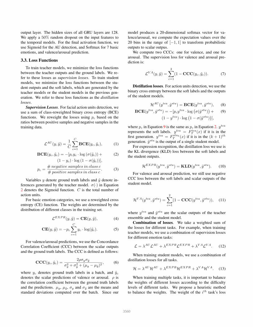
3.3. Loss Functions

To train teacher models, we minimize the loss functionsbetween the teacher outputs and the ground labels. We re-fer to these losses as supervision losses. To train studentmodels, we minimize the loss functions between the stu-dent outputs and the soft labels, which are generated by theteacher models or the student models in the previous gen-eration. We refer to these loss functions as the distillationlosses.

Supervision Losses. For facial action units detection, weuse a sum of class-reweighted binary cross entropy (BCE)functions. We reweight the losses using pc based on theratios between positive samples and negative samples in thetraining data.

LAU (y, y) =1

C

C∑c=1

BCE(yc, yc), (1)

BCE(yc, yc) = −[pcyc · log (σ(yc))+ (2)(1− yc) · log (1− σ(yc))],

pc =# negative samples in class c

# positive samples in class c. (3)

Variables y denote ground truth labels and y denote in-ferences generated by the teacher model. σ(·) in Equation2 denotes the Sigmoid function. C is the total number ofaction units.

For basic emotion categories, we use a reweighted crossentropy (CE) function. The weights are determined by thedistribution of different classes in the training set.

LEXPR(y, y) = CE(y, y), (4)

CE(y, y) = −pcC∑

c=1

yc · log(yc). (5)

For valence/arousal predictions, we use the ConcordanceCorrelation Coefficient (CCC) between the scalar outputsand the ground truth labels. The CCC is defined as follows:

CCC(yc, yc) =2ρσyσy

σ2y + σ2

y + (µy − µy)2, (6)

where yc denotes ground truth labels in a batch, and ycdenotes the scalar predictions of valence or arousal. ρ isthe correlation coefficient between the ground truth labelsand the predictions. µy , µy , σy and σy are the means andstandard deviations computed over the batch. Since our

model produces a 20-dimensional softmax vector for va-lence/arousal, we compute the expectation values over the20 bins in the range of [−1, 1] to transform probabilisticoutputs to scalar outpus.

We compute two CCCs: one for valence, and one forarousal. The supervision loss for valence and arousal pre-diction is:

LV A(y, y) =

2∑c=1

(1−CCC(yc, yc)). (7)

Distillation losses. For action units detection, we use thebinary cross entropy between the soft labels and the outputsof the student models.

HAU (ytea, ystu) = BCE(ytea, ystu), (8)

BCE(ytea, ystu) = −[pcytea · log(σ(ystu)

)+ (9)

(1− ytea) · log(1− σ(ystu)

)],

where pc in Equation 9 is the same as pc in Equation 2. ytea

represents the soft labels. ytea = F teaT (x) if it is in the

first generation. ytea = F stuk

T (x) if it is in the (k + 1)th

generation. ystu is the output of a single student model.For expression recognition, the distillation loss we use is

the KL divergence (KLD) loss between the soft labels andthe student outputs.

HEXPR(ytea, ystu) = KLD(ytea, ystu). (10)

For valence and arousal prediction, we still use negativeCCC loss between the soft labels and scalar outputs of thestudent model.

HV A(ytea, ystu) =

2∑c=1

(1−CCC(ytea, ystu)), (11)

where ytea and ystu are the scalar outputs of the teacherensemble and the student model.

Combination of losses. We take a weighted sum ofthe losses for different tasks. For example, when trainingteacher models, we use a combination of supervision lossesfor different emotion tasks:

L = λAULAU + λEXPRLEXPR + λV ALV A. (12)

When training student models, we use a combination ofdistillation losses for all tasks.

H = λAUHAU + λEXPRHEXPR + λV AHV A. (13)

When training multiple tasks, it is important to balancethe weights of different losses according to the difficultylevels of different tasks. We propose a heuristic methodto balance the weights. The weight of the ith task’s loss

3560

{𝑋, 𝑌}

𝑓1𝑡𝑒𝑎

𝑓2𝑡𝑒𝑎

𝑓3𝑡𝑒𝑎

𝑓4𝑡𝑒𝑎

𝑓5𝑡𝑒𝑎

{𝑋, 𝐹5𝑡𝑒𝑎(𝑋)} {𝑋, 𝐹5

𝑠𝑡𝑢1(𝑋)}

𝐹𝑡𝑒𝑎: the teacher ensemble𝐹𝑠𝑡𝑢1: the student ensemble

in the 1𝑠𝑡 generation𝐹𝑠𝑡𝑢2: the student ensemble

in the 2𝑛𝑑 generation

… …

𝑓1𝑠𝑡𝑢1

𝑓2𝑠𝑡𝑢1

𝑓3𝑠𝑡𝑢1

𝑓4𝑠𝑡𝑢1

𝑓5𝑠𝑡𝑢1

𝑓1𝑠𝑡𝑢2

𝑓2𝑠𝑡𝑢2

𝑓3𝑠𝑡𝑢2

𝑓4𝑠𝑡𝑢2

𝑓5𝑠𝑡𝑢2

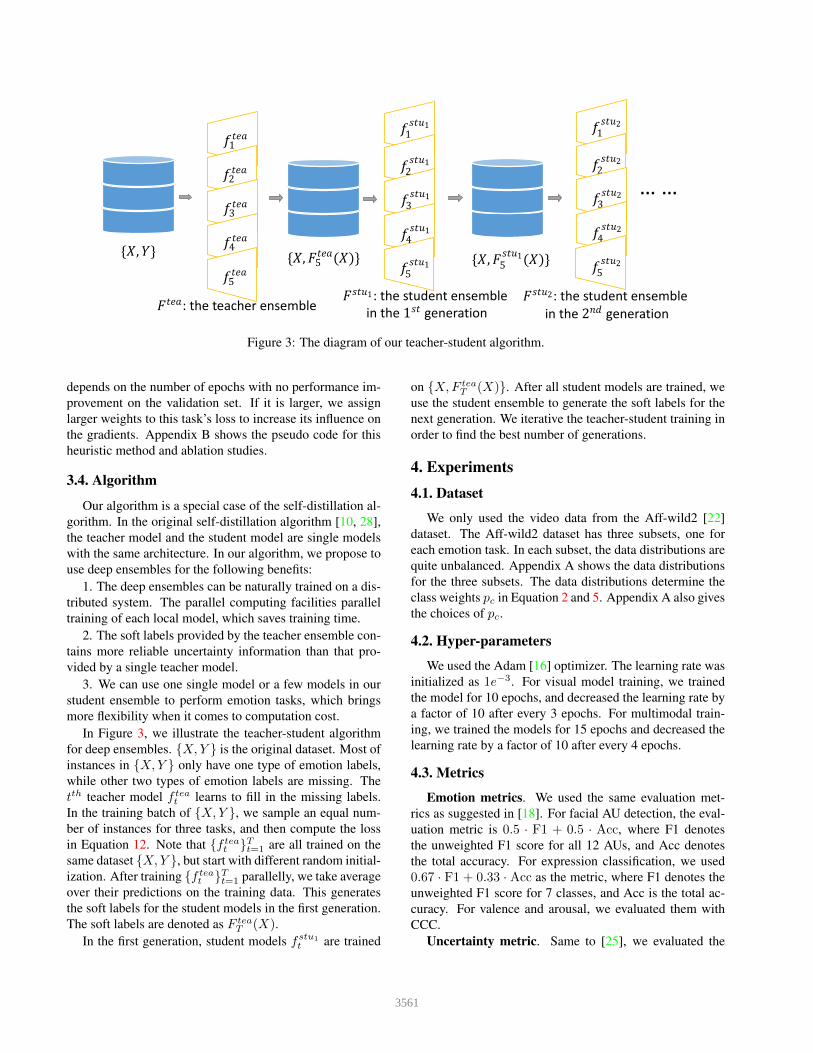
Figure 3: The diagram of our teacher-student algorithm.

depends on the number of epochs with no performance im-provement on the validation set. If it is larger, we assignlarger weights to this task’s loss to increase its influence onthe gradients. Appendix B shows the pseudo code for thisheuristic method and ablation studies.

3.4. Algorithm

Our algorithm is a special case of the self-distillation al-gorithm. In the original self-distillation algorithm [10, 28],the teacher model and the student model are single modelswith the same architecture. In our algorithm, we propose touse deep ensembles for the following benefits:

1. The deep ensembles can be naturally trained on a dis-tributed system. The parallel computing facilities paralleltraining of each local model, which saves training time.

2. The soft labels provided by the teacher ensemble con-tains more reliable uncertainty information than that pro-vided by a single teacher model.

3. We can use one single model or a few models in ourstudent ensemble to perform emotion tasks, which bringsmore flexibility when it comes to computation cost.

In Figure 3, we illustrate the teacher-student algorithmfor deep ensembles. {X,Y } is the original dataset. Most ofinstances in {X,Y } only have one type of emotion labels,while other two types of emotion labels are missing. Thetth teacher model f tea

t learns to fill in the missing labels.In the training batch of {X,Y }, we sample an equal num-ber of instances for three tasks, and then compute the lossin Equation 12. Note that {f tea

t }Tt=1 are all trained on thesame dataset {X,Y }, but start with different random initial-ization. After training {f tea

t }Tt=1 parallelly, we take averageover their predictions on the training data. This generatesthe soft labels for the student models in the first generation.The soft labels are denoted as F tea

T (X).In the first generation, student models fstu1

t are trained

on {X,F teaT (X)}. After all student models are trained, we

use the student ensemble to generate the soft labels for thenext generation. We iterative the teacher-student training inorder to find the best number of generations.

4. Experiments4.1. Dataset

We only used the video data from the Aff-wild2 [22]dataset. The Aff-wild2 dataset has three subsets, one foreach emotion task. In each subset, the data distributions arequite unbalanced. Appendix A shows the data distributionsfor the three subsets. The data distributions determine theclass weights pc in Equation 2 and 5. Appendix A also givesthe choices of pc.

4.2. Hyper-parameters

We used the Adam [16] optimizer. The learning rate wasinitialized as 1e−3. For visual model training, we trainedthe model for 10 epochs, and decreased the learning rate bya factor of 10 after every 3 epochs. For multimodal train-ing, we trained the models for 15 epochs and decreased thelearning rate by a factor of 10 after every 4 epochs.

4.3. Metrics

Emotion metrics. We used the same evaluation met-rics as suggested in [18]. For facial AU detection, the eval-uation metric is 0.5 · F1 + 0.5 · Acc, where F1 denotesthe unweighted F1 score for all 12 AUs, and Acc denotesthe total accuracy. For expression classification, we used0.67 · F1 + 0.33 · Acc as the metric, where F1 denotes theunweighted F1 score for 7 classes, and Acc is the total ac-curacy. For valence and arousal, we evaluated them withCCC.

Uncertainty metric. Same to [25], we evaluated the

3561

Tea Stu1 Stu2 Stu3 Stu42.102.152.202.252.302.352.40

Tota

l Em

otio

n M

etric

EMENet-VSingleEnsemble

Tea Stu1 Stu2 Stu3 Stu42.102.152.202.252.302.352.40

Tota

l Em

otio

n M

etric

EMENet-VASingleEnsemble

Figure 4: The total emotion metrics for the visual model(EMENet-V) and the visual-audio model (EMENet-VA), onthe validation set of the Aff-wild2. For the single models’results, we average the total emotion metric over five runs,and the standard deviations are shown with error bars. ”Tea”stands for the teacher model (ensemble). ”Stu1” stands forthe student model (ensemble) in the first generation.

in-domain uncertainty estimation performance using thenegative log-likelihood (NLL) for classification tasks (i.e.,EXPR and AU) and root mean square error (RMSE) forregression tasks (i.e., valence and arousal). Lower NLLor RMSE means better uncertainty estimation performance.For out-of-domain uncertainty performance, we created anOOD detection task by importing non-facial images, andevaluated the binary classification performance using ROC(receiver operating characteristic) curves and AUC (area un-der the ROC curve) scores.

5. Results

5.1. Task Performance

Experiments T AU EXPR VA Total EmotionValence Arousalw/o re. 1 0.6773 0.5128 0.3830 0.5268 2.0999w/o re. 5 0.6858 0.5354 0.4099 0.5537 2.1848w/o re. 10 0.6843 0.5449 0.4105 0.5577 2.1974w/ re. 1 0.6632 0.5541 0.4202 0.5192 2.1527w/ re. 5 0.6808 0.5779 0.4423 0.5455 2.2465

Table 1: Validation results with the teacher models using vi-sual modality only. ”w/ re.” means we apply class reweight-ing for EXPR and AU. T is the number of models in an en-semble. T = 1 means it is a single model. Total emotionmetric is the sum of all metrics of the three emotion tasks.

Methods # Gen. # Param. AU EXPR VAValence Arousal

EMENet-V 3 1.68M 0.6320 0.4639 0.4942 0.4355EMENet-V 3 8.4M 0.6328 0.4704 0.5104 0.4419

EMENet-VA 2 1.91M 0.6418 0.5046 0.5355 0.4442EMENet-VA 1 9.55M 0.6528 0.5041 0.5326 0.4537

Table 2: The emotion metrics on the test set of the Aff-wild2 dataset. ”# Gen.” denotes the number of generations.”# Param.” denotes the number of parameters. The enmse-bles have five times larger number of parameters than singlemodels.

Computation cost. We designed two model architec-tures for the visual modality and visual-audio modalities re-spectively. We refer to them as EMENet-V and EMENet-VA. The number of parameters and FLOPs for EMENet-Vare 1.68M and 228M . For EMENet-VA, they are 1.91Mand 234M . The FLOPs are the number of floating-point op-erations when the visual input is one RGB image (112x112)and audio input is one spectrogram (64x64).

Class reweighting. We show the effect of classreweighting in Table 1. After applying class reweighting,we found the EXPR metric for single models was improvedsignificantly, where the F1 score increased by 12.6%, andthe accuracy of EXPR increased by 1.7%. Although the AUmetric degraded after using class reweighting, its F1 scoreincreased by 12.5%. The AU metric degraded because itsaccuracy dropped from 0.8947 to 0.8249. We think this isdue to the highly unbalanced data distribution in the AUsubset.

Ensemble size. We changed the ensemble size whentraining teacher models without class reweighting. The re-sults are reported in Table 1. From single models (T = 1)to ensemble models (T = 5), the total emotion metric in-creased by 4%. However, from T = 10 to T = 5, the totalemotion metric only increased by 0.58%. We kept the en-semble size T = 5 for the rest of experiments because of itsrelative efficiency.

Teacher-Student training. We trained our teacher mod-els and student models using our proposed algorithm (Fig-ure 3). The total emotion metrics for both the teachersand students in multiple generations are shown in Figure4. Our first finding is that ensembles always outperformsingle models on the total emotion metric. As we increasedthe number of generations, the performance gap betweenthe single models and ensembles became smaller. This isprobably because the variability between models becomessmaller and smaller after more and more generations of self-distillation.

Our second finding on the results of EMENet-V is thatthe emotion performance does not increase monotonicallyas the number of generations increases. This is consistentwith [28], where they interpreted increasing generations of

3562

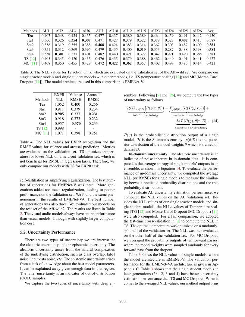
Methods AU1 AU2 AU4 AU6 AU7 AU10 AU12 AU15 AU23 AU24 AU25 AU26 Avg.Tea 0.407 0.348 0.424 0.435 0.477 0.437 0.380 0.389 0.464 0.459 0.491 0.442 0.430Stu1 0.366 0.326 0.354 0.387 0.471 0.427 0.379 0.322 0.388 0.328 0.482 0.413 0.387Stu2 0.358 0.319 0.355 0.388 0.468 0.424 0.383 0.314 0.367 0.303 0.487 0.400 0.381Stu3 0.351 0.312 0.369 0.395 0.479 0.435 0.400 0.310 0.353 0.287 0.488 0.398 0.381Stu4 0.338 0.301 0.377 0.401 0.482 0.440 0.421 0.322 0.347 0.271 0.490 0.386 0.381

TS [12] 0.405 0.345 0.420 0.435 0.476 0.435 0.379 0.388 0.462 0.449 0.491 0.441 0.427MC [11] 0.408 0.350 0.455 0.429 0.472 0.422 0.362 0.357 0.402 0.499 0.485 0.414 0.421

Table 3: The NLL values for 12 action units, which are evaluated on the validation set of the Aff-wild set. We compare oursingle teacher models and single student models with other methods, i.e., TS (temperature scaling [12]) and MC (Monte-CarolDropout [11]). The model architecture used in this comparison is EMENet-V.

MethodsEXPRNLL

ValenceRMSE

ArousalRMSE

Tea 1.052 0.400 0.256Stu1 0.911 0.379 0.234Stu2 0.905 0.377 0.231Stu3 0.918 0.373 0.232Stu4 0.957 0.370 0.233

TS [12] 0.998 - -MC [11] 1.071 0.398 0.251

Table 4: The NLL values for EXPR recognition and theRMSE values for valence and arousal prediction. Metricsare evaluated on the validation set. TS optimizes temper-ature for lower NLL on a held-out validation set, which isnot beneficial for RMSE in regression tasks. Therefore, weonly compare our models with TS for EXPR task.

self-distillation as amplifying regularization. The best num-ber of generations for EMENet-V was three. More gen-erations added too much regularization, leading to poorerperformance on the validation set. We found the same phe-nomenon in the results of EMENet-VA. The best numberof generations was also three. We evaluated our models onthe test set of the Aff-wild2. The results are listed in Table2. The visual-audio models always have better performancethan visual models, although with slightly larger computa-tion cost.

5.2. Uncertainty Performance

There are two types of uncertainty we are interest in:the aleatoric uncertainty and the epistemic uncertainty. Thealeatoric uncertainty arises from the natural complexitiesof the underlying distribution, such as class overlap, labelnoise, input data noise, etc. The epistemic uncertainty arisesfrom a lack of knowledge about the best model parameters.It can be explained away given enough data in that region.The latter uncertainty is an indicator of out-of-distribution(OOD) samples.

We capture the two types of uncertainty with deep en-

sembles. Following [9] and [26], we compute the two typesof uncertainty as follows:

H(Ep(θ|D) [P (y|x, θ)])︸ ︷︷ ︸total uncertainty

= Ep(θ|D) [H(P (y|x, θ)]︸ ︷︷ ︸aleatoric uncertainty

+

MI [P (y), θ|x,D]︸ ︷︷ ︸epistemic uncertainty

. (14)

P (y) is the probabilistic distribution output of a singlemodel. H is the Shannon’s entropy. p(θ|D) is the poste-rior distribution of the model weights θ which is trained ondataset D.

In-domain uncertainty. The aleatoric uncertainty is anindicator of noise inherent in in-domain data. It is com-puted as the average entropy of single models’ outputs in anensemble, as shown in Equation 14. To evaluate the perfor-mance of in-domain uncertainty, we computed the averageNLL (or RMSE) for single models to measure the similar-ity between predicted probability distributions and the trueprobability distributions.

To evaluate AU uncertainty estimation performance, wecomputed the NLL values on the AU validation set. Be-sides the NLL values of our single teacher models and sin-gle student models, the NLLs values of Temperature scal-ing (TS) [12] and Monte-Carol Dropout (MC Dropout) [11]were also computed. For a fair comparison, we adoptedthe test-time cross-validation in [1] to compute the NLL inTS. The optimal temperature was optimized on a randomly-split half of the validation set. The NLL was then evaluatedon the other half of the validation set. For MC Dropout,we averaged the probability outputs of ten forward passes,where the model weights were sampled randomly for everyforward pass from the dropout.

Table 3 shows the NLL values of single models, wherethe model architecture is EMENet-V. The validation per-formance for the EMENet-VA architecture is given in Ap-pendix C. Table 3 shows that the single student models inlater generations (i.e., 2, 3 and 4) have better uncertaintyestimation performance than TS and MC Dropout. When itcomes to the averaged NLL values, our method outperforms

3563

TS by 10.8% and MC Dropout by 9.5%.

In Table 4, we list the uncertainty metrics for facial ex-pressions (EXPR), valence and arousal. We find that thesingle student models have better uncertainty performancethan TS and MC Dropout for both tasks. Our algorithm im-proves the EXPR NLL by 10.3% when compared with TSand 15.5% when compared with MC Dropout. As for va-lence/arousal RMSE scores, our method outperforms MCDropout by 7.0%/8.0%.

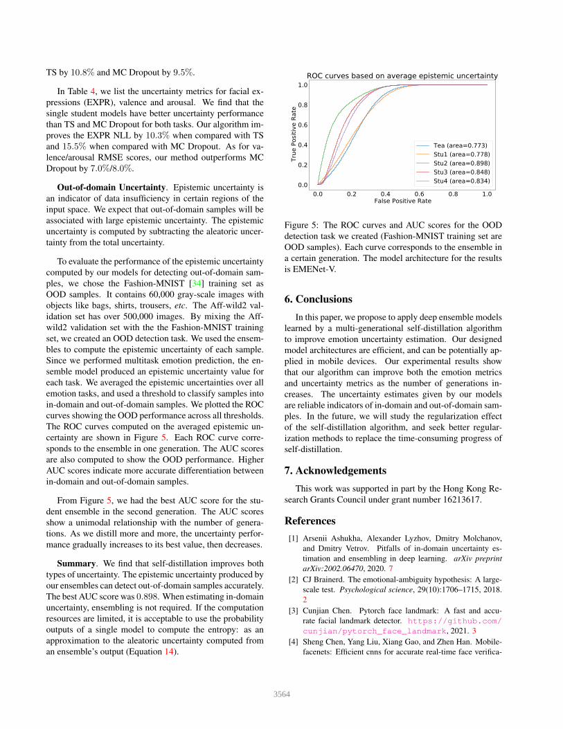
Out-of-domain Uncertainty. Epistemic uncertainty isan indicator of data insufficiency in certain regions of theinput space. We expect that out-of-domain samples will beassociated with large epistemic uncertainty. The epistemicuncertainty is computed by subtracting the aleatoric uncer-tainty from the total uncertainty.

To evaluate the performance of the epistemic uncertaintycomputed by our models for detecting out-of-domain sam-ples, we chose the Fashion-MNIST [34] training set asOOD samples. It contains 60,000 gray-scale images withobjects like bags, shirts, trousers, etc. The Aff-wild2 val-idation set has over 500,000 images. By mixing the Aff-wild2 validation set with the the Fashion-MNIST trainingset, we created an OOD detection task. We used the ensem-bles to compute the epistemic uncertainty of each sample.Since we performed multitask emotion prediction, the en-semble model produced an epistemic uncertainty value foreach task. We averaged the epistemic uncertainties over allemotion tasks, and used a threshold to classify samples intoin-domain and out-of-domain samples. We plotted the ROCcurves showing the OOD performance across all thresholds.The ROC curves computed on the averaged epistemic un-certainty are shown in Figure 5. Each ROC curve corre-sponds to the ensemble in one generation. The AUC scoresare also computed to show the OOD performance. HigherAUC scores indicate more accurate differentiation betweenin-domain and out-of-domain samples.

From Figure 5, we had the best AUC score for the stu-dent ensemble in the second generation. The AUC scoresshow a unimodal relationship with the number of genera-tions. As we distill more and more, the uncertainty perfor-mance gradually increases to its best value, then decreases.

Summary. We find that self-distillation improves bothtypes of uncertainty. The epistemic uncertainty produced byour ensembles can detect out-of-domain samples accurately.The best AUC score was 0.898. When estimating in-domainuncertainty, ensembling is not required. If the computationresources are limited, it is acceptable to use the probabilityoutputs of a single model to compute the entropy: as anapproximation to the aleatoric uncertainty computed froman ensemble’s output (Equation 14).

0.0 0.2 0.4 0.6 0.8 1.0False Positive Rate

0.0

0.2

0.4

0.6

0.8

1.0

True

Pos

itive

Rat

e

ROC curves based on average epistemic uncertainty

Tea (area=0.773)Stu1 (area=0.778)Stu2 (area=0.898)Stu3 (area=0.848)Stu4 (area=0.834)

Figure 5: The ROC curves and AUC scores for the OODdetection task we created (Fashion-MNIST training set areOOD samples). Each curve corresponds to the ensemble ina certain generation. The model architecture for the resultsis EMENet-V.

6. ConclusionsIn this paper, we propose to apply deep ensemble models

learned by a multi-generational self-distillation algorithmto improve emotion uncertainty estimation. Our designedmodel architectures are efficient, and can be potentially ap-plied in mobile devices. Our experimental results showthat our algorithm can improve both the emotion metricsand uncertainty metrics as the number of generations in-creases. The uncertainty estimates given by our modelsare reliable indicators of in-domain and out-of-domain sam-ples. In the future, we will study the regularization effectof the self-distillation algorithm, and seek better regular-ization methods to replace the time-consuming progress ofself-distillation.

7. AcknowledgementsThis work was supported in part by the Hong Kong Re-

search Grants Council under grant number 16213617.

References[1] Arsenii Ashukha, Alexander Lyzhov, Dmitry Molchanov,

and Dmitry Vetrov. Pitfalls of in-domain uncertainty es-timation and ensembling in deep learning. arXiv preprintarXiv:2002.06470, 2020. 7

[2] CJ Brainerd. The emotional-ambiguity hypothesis: A large-scale test. Psychological science, 29(10):1706–1715, 2018.2

[3] Cunjian Chen. Pytorch face landmark: A fast and accu-rate facial landmark detector. https://github.com/cunjian/pytorch_face_landmark, 2021. 3

[4] Sheng Chen, Yang Liu, Xiang Gao, and Zhen Han. Mobile-facenets: Efficient cnns for accurate real-time face verifica-

3564

tion on mobile devices. In Chinese Conference on BiometricRecognition, pages 428–438. Springer, 2018. 3

[5] Ting Dang, Vidhyasaharan Sethu, Julien Epps, andEliathamby Ambikairajah. An investigation of emotion pre-diction uncertainty using gaussian mixture regression. In IN-TERSPEECH, pages 1248–1252, 2017. 2

[6] Ting Dang, Brian Stasak, Zhaocheng Huang, SadariJayawardena, Mia Atcheson, Munawar Hayat, Phu Le, Vid-hyasaharan Sethu, Roland Goecke, and Julien Epps. Inves-tigating word affect features and fusion of probabilistic pre-dictions incorporating uncertainty in avec 2017. In Proceed-ings of the 7th Annual Workshop on Audio/Visual EmotionChallenge, pages 27–35, 2017. 2

[7] Didan Deng, Zhaokang Chen, and Bertram E Shi. Multitaskemotion recognition with incomplete labels. In 2020 15thIEEE International Conference on Automatic Face and Ges-ture Recognition (FG 2020), pages 592–599. IEEE, 2020. 2,3

[8] Didan Deng, Zhaokang Chen, Yuqian Zhou, and BertramShi. Mimamo net: Integrating micro-and macro-motion forvideo emotion recognition. In Proceedings of the AAAI Con-ference on Artificial Intelligence, volume 34, pages 2621–2628, 2020. 3

[9] Stefan Depeweg, Jose-Miguel Hernandez-Lobato, FinaleDoshi-Velez, and Steffen Udluft. Decomposition of un-certainty in bayesian deep learning for efficient and risk-sensitive learning. In International Conference on MachineLearning, pages 1184–1193. PMLR, 2018. 7

[10] Tommaso Furlanello, Zachary Lipton, Michael Tschannen,Laurent Itti, and Anima Anandkumar. Born again neural net-works. In International Conference on Machine Learning,pages 1607–1616. PMLR, 2018. 2, 5

[11] Yarin Gal and Zoubin Ghahramani. Dropout as a bayesianapproximation: Representing model uncertainty in deeplearning. In international conference on machine learning,pages 1050–1059. PMLR, 2016. 2, 7, 12

[12] Chuan Guo, Geoff Pleiss, Yu Sun, and Kilian Q Weinberger.On calibration of modern neural networks. In InternationalConference on Machine Learning, pages 1321–1330. PMLR,2017. 2, 7, 12

[13] Jing Han, Zixing Zhang, Maximilian Schmitt, Maja Pantic,and Bjorn Schuller. From hard to soft: Towards more human-like emotion recognition by modelling the perception uncer-tainty. In Proceedings of the 25th ACM international confer-ence on Multimedia, pages 890–897, 2017. 1, 2

[14] Geoffrey Hinton, Oriol Vinyals, and Jeff Dean. Distill-ing the knowledge in a neural network. arXiv preprintarXiv:1503.02531, 2015. 2

[15] Fei Jia, Somshubra Majumdar, and Boris Ginsburg. Mar-blenet: Deep 1d time-channel separable convolutional neu-ral network for voice activity detection. In ICASSP 2021-2021 IEEE International Conference on Acoustics, Speechand Signal Processing (ICASSP), pages 6818–6822. IEEE,2021. 3

[16] Diederik P Kingma and Jimmy Ba. Adam: A method forstochastic optimization. arXiv preprint arXiv:1412.6980,2014. 5

[17] Dimitrios Kollias, Irene Kotsia, Elnar Hajiyev, and StefanosZafeiriou. Analysing affective behavior in the second abaw2competition. arXiv preprint arXiv:2106.15318, 2021. 2

[18] Dimitrios Kollias, Attila Schulc, Elnar Hajiyev, and StefanosZafeiriou. Analysing affective behavior in the first abaw2020 competition. In 2020 15th IEEE International Confer-ence on Automatic Face and Gesture Recognition (FG 2020),pages 637–643. IEEE, 2020. 5

[19] Dimitrios Kollias, Viktoriia Sharmanska, and StefanosZafeiriou. Face behavior a la carte: Expressions, af-fect and action units in a single network. arXiv preprintarXiv:1910.11111, 2019. 3

[20] Dimitrios Kollias, Viktoriia Sharmanska, and StefanosZafeiriou. Distribution matching for heterogeneous multi-task learning: a large-scale face study. arXiv preprintarXiv:2105.03790, 2021. 2

[21] Dimitrios Kollias, Panagiotis Tzirakis, Mihalis A Nicolaou,Athanasios Papaioannou, Guoying Zhao, Bjorn Schuller,Irene Kotsia, and Stefanos Zafeiriou. Deep affect predictionin-the-wild: Aff-wild database and challenge, deep architec-tures, and beyond. International Journal of Computer Vision,127(6):907–929, 2019. 2

[22] Dimitrios Kollias and Stefanos Zafeiriou. Aff-wild2: Ex-tending the aff-wild database for affect recognition. arXivpreprint arXiv:1811.07770, 2018. 2, 5

[23] Dimitrios Kollias and Stefanos Zafeiriou. Expression, affect,action unit recognition: Aff-wild2, multi-task learning andarcface. arXiv preprint arXiv:1910.04855, 2019. 3

[24] Dimitrios Kollias and Stefanos Zafeiriou. Affect analysisin-the-wild: Valence-arousal, expressions, action units and aunified framework. arXiv preprint arXiv:2103.15792, 2021.2

[25] Balaji Lakshminarayanan, Alexander Pritzel, and CharlesBlundell. Simple and scalable predictive uncertaintyestimation using deep ensembles. arXiv preprintarXiv:1612.01474, 2016. 2, 5

[26] Andrey Malinin, Bruno Mlodozeniec, and Mark Gales.Ensemble distribution distillation. arXiv preprintarXiv:1905.00076, 2019. 7

[27] S Mohammad Mavadati, Mohammad H Mahoor, KevinBartlett, Philip Trinh, and Jeffrey F Cohn. Disfa: A spon-taneous facial action intensity database. IEEE Transactionson Affective Computing, 4(2):151–160, 2013. 1, 2

[28] Hossein Mobahi, Mehrdad Farajtabar, and Peter L Bartlett.Self-distillation amplifies regularization in hilbert space.arXiv preprint arXiv:2002.05715, 2020. 2, 5, 6

[29] Ali Mollahosseini, Behzad Hasani, and Mohammad H Ma-hoor. Affectnet: A database for facial expression, valence,and arousal computing in the wild. IEEE Transactions onAffective Computing, 10(1):18–31, 2017. 1

[30] Emily Mower, Angeliki Metallinou, Chi-Chun Lee, AbeKazemzadeh, Carlos Busso, Sungbok Lee, and ShrikanthNarayanan. Interpreting ambiguous emotional expressions.In 2009 3rd International Conference on Affective Comput-ing and Intelligent Interaction and Workshops, pages 1–8.IEEE, 2009. 1

3565

[31] Rafael Muller, Simon Kornblith, and Geoffrey Hinton.When does label smoothing help? arXiv preprintarXiv:1906.02629, 2019. 2

[32] Yaniv Ovadia, Emily Fertig, Jie Ren, Zachary Nado, DavidSculley, Sebastian Nowozin, Joshua V Dillon, Balaji Laksh-minarayanan, and Jasper Snoek. Can you trust your model’suncertainty? evaluating predictive uncertainty under datasetshift. arXiv preprint arXiv:1906.02530, 2019. 2

[33] Michel F Valstar, Timur Almaev, Jeffrey M Girard, GaryMcKeown, Marc Mehu, Lijun Yin, Maja Pantic, and Jef-frey F Cohn. Fera 2015-second facial expression recogni-tion and analysis challenge. In 2015 11th IEEE InternationalConference and Workshops on Automatic Face and GestureRecognition (FG), volume 6, pages 1–8. IEEE, 2015. 1, 2

[34] Han Xiao, Kashif Rasul, and Roland Vollgraf. Fashion-mnist: a novel image dataset for benchmarking machinelearning algorithms. arXiv preprint arXiv:1708.07747, 2017.8

[35] Qizhe Xie, Minh-Thang Luong, Eduard Hovy, and Quoc VLe. Self-training with noisy student improves imagenet clas-sification. In Proceedings of the IEEE/CVF Conference onComputer Vision and Pattern Recognition, pages 10687–10698, 2020. 2

[36] Stefanos Zafeiriou, Dimitrios Kollias, Mihalis A Nicolaou,Athanasios Papaioannou, Guoying Zhao, and Irene Kotsia.Aff-wild: valence and arousal’in-the-wild’challenge. In Pro-ceedings of the IEEE conference on computer vision and pat-tern recognition workshops, pages 34–41, 2017. 1

[37] Zixing Zhang, Florian Eyben, Jun Deng, and Bjorn Schuller.An agreement and sparseness-based learning instance selec-tion and its application to subjective speech phenomena. InProceedings of the 5th International Workshop on EmotionSocial Signals, Sentiment & Linked Open Data (ES3LOD2014), satellite of the 9th Language Resources and Evalu-ation Conference (LREC 2014)(B. Schuller, P. Buitelaar, L.Devillers, C. Pelachaud, T. Declerck, A. Batliner, P. Rosso,and S. Gaines, eds.), Reykjavik, Iceland, 2014. 2

[38] Zhanpeng Zhang, Ping Luo, Chen Change Loy, and XiaoouTang. From facial expression recognition to interpersonal re-lation prediction. International Journal of Computer Vision,126(5):550–569, 2018. 1, 2

[39] Zhilu Zhang and Mert R Sabuncu. Self-distillationas instance-specific label smoothing. arXiv preprintarXiv:2006.05065, 2020. 2

3566