iterative leakage-based precoding for multiuser-mimo ... · convergence of the algorithm when using...

Iterative Leakage-Based Precoding for Multiuser-MIMO Systems

Eric Sollenberger

Thesis submitted to the faculty of the Virginia Polytechnic Institute and State University

in partial fulfillment of the requirements for the degree of

Master of Science

In

Electrical Engineering

Michael Buehrer

Carl Dietrich

Harpreet Dhillon

May 5, 2016

Blacksburg, VA

Keywords: multiuser, MIMO, linear precoding, leakage, imperfect CSI, LTE-A

Copyright 2016, Eric Sollenberger


Eric Sollenberger

ABSTRACT

This thesis investigates the application of an iterative leakage-based precoding algorithm

to practical multiuser-MIMO systems. We consider the effect of practical impairments

including imperfect channel state information, transmit antenna correlation, and time-

varying channels. Solutions are derived which improve performance of the algorithm

with imperfect channel state information at the transmitter by leveraging knowledge of

the second-order statistics of the error. From this work we draw a number of conclusions

on how imperfect channel state information may impact the system design including the

importance of interference suppression at the receiver and the selection of the number of

co-scheduled users. We also demonstrate an efficient approach to improve the

convergence of the algorithm when using interference-rejection-combining receivers.

Finally, we conduct simulations of an LTE-A system employing the improved algorithm

to show its utility for modern communication systems.


Eric Sollenberger

General Audience Abstract

This thesis investigates several aspects of a particular method by which multiple users

can share radio resources within a wireless system i.e. they may operate on the same

frequency and at the same time. This is a desirable capability in modern wireless systems

because it improves the efficiency of radio spectrum usage. Radio spectrum has become a

very expensive resource in recent years so achieving high efficiency is crucial. Our

investigation led us to propose several modifications to the aforementioned method

which demonstrated improved performance under certain practical conditions. We further

demonstrated the effects of several common system impairments and provided insight

into how these impairments effect the system design. Finally, we demonstrated that using

this method provides significant gains when used for the latest cellular technology.

iv

Acknowledgements

To my advisor Dr. R. Michael Buehrer, I thank you for giving me the opportunity to

work with you on this thesis. Your insight and guidance have been instrumental in

ensuring its quality and to my personal growth as a researcher in the field of wireless

communications. I have always left our weekly meetings with a renewed sense of

purpose and focus. The course I took with you on MIMO systems brought clarity to this

complex subject matter thanks to your superb teaching abilities and willingness to work

with your students.

To the members of my committee, Dr. Carl Dietrich and Dr. Dhillon, I thank you for your

advice and support over the past two years. Your mentorship has been a great help in

navigating my life as a graduate student. My understanding of wireless communications

fundamentals and software-defined radio have benefitted greatly from the courses I’ve

taken with you and the discussions we’ve had.

To my parents, I thank you for your unconditional love and support and the role-models

you have been for me. I would not have made it to this point if it weren’t for you.

v

Contents

ABSTRACT ........................................................................................................................ ii

Acknowledgements ............................................................................................................ iii

List of Abbreviations ........................................................................................................ vii

List of Figures ................................................................................................................... vii

1 Introduction ...................................................................................................................... 1

1.1 Contributions and Main Findings ............................................................................. 3

1.2 System Model ........................................................................................................... 5

1.2.1 Mathematical Annotation................................................................................... 6

1.2.2 General Assumptions ......................................................................................... 6

1.2.3 The MU-MIMO System .................................................................................... 8

1.2.4 Sum-rate of the MU-MIMO System ................................................................ 10

2 Background: Conventional MU-MIMO Techniques ..................................................... 13

2.1 Receiver Architectures ............................................................................................ 13

2.1.1 Matched Filter Receiver:.................................................................................. 14

2.1.2 Zero Forcing Receiver: .................................................................................... 15

2.1.3 Minimum Mean Squared Error Receiver: ........................................................ 15

2.1.4 Interference Rejection Combining Receiver: ................................................... 15

2.2 Conventional MU-MIMO Precoding ...................................................................... 16

2.2.1 Complete Channel Diagonalization ................................................................. 17

2.2.2 Block-Diagonal Zero-Forcing .......................................................................... 17

2.2.3 Signal-to-Leakage-and Noise Ratio Precoding ................................................ 20

2.3 Iterative Signal-to-Leakage-and-Noise Ratio Precoding ........................................ 24

2.4 Chapter Summary ................................................................................................... 32

3 Imperfect Channel State Information............................................................................. 33

3.1 SLNR Precoding Considering CSIT Error ............................................................. 33

3.1.1 Revisiting the Existing SLNR Solution ........................................................... 34

3.1.2 MMSE Modification of CSIT for SLNR Precoding ........................................ 38

3.2 iSLNR Precoding Considering CSIT Error ............................................................ 44

3.2.1 Receiver Calculation with Imperfect CSIT...................................................... 45

vi

3.2.2 Modified SLNR Precoding with Imperfect CSIT ............................................ 51

3.2.3 Simulation Results ........................................................................................... 54

3.2.4 MMSE Modification of CSIT for iSLNR Precoding ....................................... 58

3.3 iSLNR Precoding with Imperfect CSIR ................................................................. 59

3.4 Chapter Summary ................................................................................................... 63

4 Additional Considerations ............................................................................................. 66

4.1 The Effect of Transmit Antenna Correlation .......................................................... 66

4.2 Time-Varying Channels .......................................................................................... 70

4.3 Improved Convergence of the iSLNR Algorithm for IRC Receivers..................... 75

4.4 Selecting the Number of Co-Scheduled Users........................................................ 81

4.5 Conclusions ............................................................................................................. 85

5 iSLNR for LTE-A .......................................................................................................... 87

5.1 MU-MIMO in LTE-A ............................................................................................. 87

5.1.1 Downlink Waveform ....................................................................................... 87

5.1.2 MU-MIMO Transmission Modes .................................................................... 88

5.1.3 MU-MIMO Channel Estimation ...................................................................... 89

5.2 Simulated Performance ........................................................................................... 91

5.3 Conclusions ............................................................................................................. 95

6 Conclusion ..................................................................................................................... 96

References ......................................................................................................................... 98

Appendix A: Additional Transmit Antenna Correlation Simulations ............................ 100

vii

List of Abbreviations

BD-ZF

BER

BLER

CSIT

CSIR

cSLNR

DMRS

eNB

FFT

HARQ

IFFT

IRC

iSLNR

LS

LTE-A

MF

MIMO

MMSE

MSE

mSLNR

MUI

MU-MIMO

OFDM

QAM

QPSK

RB

SINR

SLNR

SNR

SU-MIMO

TM

UE

ZF

Block-diagonal zero-forcing

Bit error rate

Block error rate

Channel state information at the transmitter

Channel state information at the receiver

Conventional signal-to-leakage-and-noise ratio

Demodulation reference signals

Evolved Node B

Fast Fourier transform

Hybrid automatic repeat request

Inverse fast Fourier transform

Interference-rejection-combining

Iterative signal-to-leakage-and-noise-ratio

Least squares

Long Term Evolution Advanced

Matched filter

Multiple-input-multiple-output

Minimum mean square error

Mean square error

Modified signal-to-leakage-and-noise ratio

Multiuser-interference

Multiuser multiple-input-multiple-output

Orthogonal frequency division multiplexing

Quadrature amplitude modulation

Quadrature phase shift keying

Resource block

Signal-to-interference-and-noise ratio

Signal-to-leakage-and-noise ratio

Signal-to-noise ratio

Single-user multiple-input-multiple-output

Transmission mode

User equipment

Zero-forcing

vii

List of Figures Figure 1.1: MU-MIMO system block diagram ................................................................. 10

Figure 2.1: BER using ZF and BD-ZF precoding schemes .............................................. 20

Figure 2.2: BER using BD-ZF and SLNR precoding schemes ........................................ 23

Figure 2.3: BER error floor using SLNR precoding with 𝑁 < 𝑖 = 1𝐾𝑀𝑖 ....................... 24

Figure 2.4: Sum-rate achieved using iSLNR in a 4x(2x2) system with 20 dB SNR ........ 27

Figure 2.5: Sum-rate achieved using iSLNR in a 4x(2x4) system with 20 dB SNR ........ 28

Figure 2.6: Convergence behavior for sum-rate achieved using iSLNR in a 4x(2x4)

system with 20 dB SNR .................................................................................................... 29

Figure 2.7: Sum-rate of 9x(3x3) system using iSLNR precoding with IRC receivers at 0

dB SNR ............................................................................................................................. 30

Figure 2.8: Sum-rate of 9x(3x3) system using iSLNR precoding with IRC receivers at 30

dB SNR ............................................................................................................................. 30

Figure 2.9: BER for a 4x(2x4) system using iSLNR and ZF receivers ............................ 31

Figure 2.10: BER for a 4x(2x4) system using iSLNR and IRC receivers ........................ 31

Figure 3.1: BER comparison between SLNR precoding considering CSIT error using the

existing solution and the newly derived solution for a 9x(3x3) system ........................... 38

Figure 3.2: MMSE Modified CSIT Mean Square Error ................................................... 43

Figure 3.3: Bit error rate with MMSE modification of CSIT ........................................... 44

Figure 3.4 Sum-rate achieved using iSLNR in a 4x(2x4) system with 30 dB SNR and 10

dB CSIT ............................................................................................................................ 55

Figure 3.5: BER of a 8x(4x4) system using iSLNR for 64 QAM transmission operating

with 10 dB CSIT ............................................................................................................... 56

Figure 3.6: BER of a 8x(2x4) system using iSLNR for QPSK transmission operating with

10 dB CSIT ....................................................................................................................... 57

Figure 3.7: Sum-rate of a 16x(2x8) system using iSLNR operating at 30 dB SNR and 10

dB CSIT ............................................................................................................................ 58

Figure 3.8: BER using iSLNR precoding with and without the MMSE modified CSIT . 59

Figure 3.9: Sum-rate achieved in a 9x(3x3) system operating at 20 dB SNR and with

varying quality of CSIR .................................................................................................... 61

viii

Figure 3.10: Sum-rate achieved in a 9x(3x3) system operating at 10 dB SNR with varying

quality of CSIR ................................................................................................................. 61





Figure 4.1: Sum-rate of 8x(2x4) system with varying transmit correlation ..................... 68

Figure 4.2: Sum-rate of 4x(2x4) system with varying transmit correlation ..................... 69

Figure 4.3: Sum-rate of 4x(2x4) system using ZF receivers with varying transmit

correlation ......................................................................................................................... 69

Figure 4.4: 10 Hz max Doppler channel correlation over a 140 symbol frame with a

duration of 10 ms. ............................................................................................................. 71

Figure 4.5: 10 Hz max Doppler CSIT error variance due to a time-varying channel. ...... 72

Figure 4.6: Sum-rate of a 4x(2x4) system in a time-varying channel .............................. 74

Figure 4.7: Sum-rate of a 16x(2x8) system in a time-varying channel ............................ 75

Figure 4.8: Sum-rate using the iSLNR algorithm for IRC and ZF receivers but employing

IRC receivers .................................................................................................................... 77

Figure 4.9: Sum-rate of a 4x(2x4) system using the fast-converging iSLNR algorithm

with 𝑛𝑍𝐹 = 50 ................................................................................................................. 78

Figure 4.10: Sum-rate of a 4x(2x4) system using the fast-converging iSLNR algorithm

with 𝑛𝑍𝐹 = 5 .................................................................................................................... 79

Figure 4.11: Sum-rate of a 9x(3x3) system using both the standard and fast-converging

iSLNR algorithms with and without consideration to CSIT error .................................... 80

Figure 4.12: Sum-rate of a 16x(2x8) system using both the standard and fast-converging

iSLNR algorithms with and without consideration to CSIT error .................................... 81

Figure 4.13: Sum-rate vs. SNR of a 4x(2xK) system operating with perfect CSIT with

IRC receivers .................................................................................................................... 82

Figure 4.14: Sum-rate vs. SNR of a 4x(2xK) system operating with 10 dB CSIT with IRC

receivers ............................................................................................................................ 83

Figure 4.15: Sum-rate vs. SNR of a 4x(2xK) system operating with 10 dB CSIT ........... 84

Figure 4.16: Sum-rate vs. SNR of a 8x(2xK) system operating with Perfect CSIT ......... 85

ix

Figure 4.17: Sum-rate vs. SNR of a 8x(2xK) system operating with 10 dB CSIT ........... 85

Figure 5.1: Block diagram of MIMO-OFDM system ....................................................... 88

Figure 5.2: DMRS mapping to the resource grid .............................................................. 90

Figure 5.3: Uncoded BER of LTE-A using iSLNR with LS channel estimation ............. 92

Figure 5.4: BLER of LTE-A using iSLNR with LS channel estimation .......................... 92

Figure 5.5: Throughput of LTE-A using iSLNR with LS channel estimation ................. 93

Figure 5.6: Uncoded BER of LTE-A using iSLNR with MMSE channel estimation ...... 94

Figure 5.7: BLER of LTE-A using iSLNR with MMSE channel estimation ................... 94

Figure 5.8: Throughput of LTE-A using iSLNR with MMSE channel estimation .......... 95

Figure 8.1: Sum-rate of 6x(3x3) system with varying transmit correlation ................... 100



Figure 8.4: Sum-rate of 12x(3x4) system with varying transmit correlation ................. 101



Figure 8.7: Sum-rate of 6x(3x3) system with ZF receivers and varying transmit

correlation ....................................................................................................................... 103


correlation ....................................................................................................................... 103


correlation ....................................................................................................................... 104

1

Chapter 1

Introduction

In recent years there has been significant work done in the area of multi-user multiple-

input multiple-output (MU-MIMO) techniques for wireless communication systems.

Ideally MU-MIMO will achieve significant system sum-rate gains compared to single-

user MIMO (SU-MIMO) by spatially multiplexing multiple users onto a common set of

radio resources. Indeed MU-MIMO has already been incorporated into some of the more

prominent wireless standards e.g., LTE [1] and IEEE 802.11 [2], and some of the

promised gains have been realized. That being said, there are still improvements that can

be made to realize the full potential of MU-MIMO. For the downlink, one of the most

pressing design challenges is efficiently suppressing the multi-user interference that will

naturally occur between co-channel users using the spatial degrees of freedom afforded

from having multiple transmit antennas. While it is well known that Dirty Paper Coding

(DPC), originally proposed in [3], is the optimal precoding technique in terms of sum-rate,

it is typically considered to be prohibitively complex. For this reason, suboptimal but

much lower-complexity linear precoding schemes are an attractive alternative.

A number of linear precoding schemes have been proposed based on various optimization

criteria. Zero-forcing and block-diagonal zero-forcing [4] constrain the problem to create

zero multiuser-interference (MUI). This is accomplished by ensuring that the precoding

matrix for each user lies in the null-space of the channel for all other users. While zero

MUI sounds good, these schemes give no consideration to the noise present at the

receivers which degrades their performance. Regularized zero-forcing schemes have been

proposed as a way of accounting for the noise in the low SNR regime [5]. The concept of

leakage-based precoding was proposed in [6] and later extended to consider noise using

the signal-to-leakage-and-noise ratio (SLNR) metric [7]. The solution presented in [7] is

referred to as the conventional SLNR precoding scheme (cSLNR) in this thesis. The

SLNR metric is useful in that it is closely related to the signal-to-interference-and-noise

ratio (SINR) which ultimately determines the performance of the wireless links, but it

2

decouples the user precoding matrices which can be problematic for SINR maximization

schemes. It also has the benefit of not requiring the number of transmit antennas to be

equal to or greater than the total number of receive antennas, whereas the other schemes

mentioned do impose such a requirement. The SLNR metric was used in an iterative

algorithm (iSLNR) in [8] which considers the receiver processing and provides substantial

gains for non-full-rank transmissions. Another iterative approach was described in [9]

which considers the MUI imposed on the user in addition to the leaked MUI, though this

approach did not show as significant results. These schemes will be discussed in greater

detail in a later section.

Interference suppression at the receiver can provide further gains when there is residual

MUI after precoding. Receivers with this capability are referred to as interference-aware,

whereas other receivers are interference-unaware. Interference-aware receivers include the

interference-rejection-combining (IRC) receiver and the Max-log-MAP receiver [10].

Interference-unaware receivers include any of the traditional single-user receiver

structures such as the matched-filter (MF), zero-forcing (ZF), and minimum-mean-square-

error (MMSE) receivers. To be clear, the single-user ZF and MMSE receivers will

suppress interference between multiple streams for a single user, but do not consider

interference from other users’ streams. The work in [10,11] demonstrated that when

precoding matrices are quantized to a finite codebook, the interference-aware receivers

provide significant gains over the interference-unaware receivers due to the residual MUI.

The transmitter and receiver techniques discussed above rely on accurate channel state

information at the transmitter (CSIT) and at the receiver (CSIR) respectively to achieve

good performance. Imperfect CSIT and/or CSIR can lead to significant system

performance degradation. Since any practical system will have some degree of

CSIT/CSIR error, these are compelling issues to consider. CSIT error can result as a

culmination of several factors including channel estimation error, acquisition delay, non-

reciprocal hardware, and time-varying channels. For this reason CSIT quality may not

necessarily track with SNR. CSIR quality on the other hand, is often considered to track

the SNR rather closely, particularly with low Doppler spread.

3

In this work we focus our attention on application of the iSLNR algorithm in a practical

setting, that is, with practical system impairments and using techniques employed by

current communications systems. We begin by considering the impairment of imperfect

CSIT and CSIR. We then consider transmit antenna correlation and time-varying

channels. Finally, we investigate the application of the iSLNR algorithm to an LTE-A

system.

1.1 Contributions and Main Findings

In this section we summarize the contributions and main findings presented in this thesis.

Conventional SLNR Precoding with Imperfect CSIT: We derive the solution

for the precoding matrix which will maximize the SLNR in the presence of

imperfect CSIT. We note that this problem was previously addressed in [7] using

the same model for the imperfect CSIT, however our derivation leads us to a

slightly different solution which is shown to provide better performance.

iSLNR Precoding with Imperfect CSIT: The iSLNR algorithm will be degraded

in two ways due to imperfect CSIT. First, there will be error between the receive

filters calculated at the transmitter during the execution of the iSLNR algorithm

and those actually employed at the receiver. The calculation of the precoding

matrix will also be affected in a manner similar to the cSLNR scheme. By using

the MMSE estimate of the receive filters and modifying the precoding matrix

calculation we are able to improve performance of the iSLNR algorithm with

imperfect CSIT.

MMSE Modification of CSIT: The work in [12, 20] motivated us to investigate

potential performance gains that might be realized by applying a linear

modification to the CSIT so as to minimize its mean square error with respect to

the true channel. We note that the solution presented in [12, 20] is not suitable for

a practical system as the modification depends on knowledge of the true channel

while the transmitter will only possess an estimate of the channel. We therefore

derive the MMSE modification that avoids relying on the true channel, which

4

turns out to be a simple scalar factor. We apply this modification to both the

conventional and iterative SLNR precoding schemes. It was shown to provide

some marginal though non-negligible gain to the conventional scheme, though

this gain did not translate to the iterative algorithm.

iSLNR Precoding with Imperfect CSIR: It was shown that imperfect CSIR will

lead to performance degradation for the iSLNR algorithm which relies on

knowledge of the receive filters. At a sufficiently poor quality CSIR, the iSLNR

algorithm actually performs worse than the cSLNR solution. Simulations showed

that for systems where the number of transmit antennas is greater than or equal to

the total number of receive antennas for all users the CSIR quality should be

greater than the SNR in order to achieve significant gain using the iSLNR

algorithm. For systems where the number of transmit antennas is less than the

total number of receive antennas for all users this requirement is not as strict.

iSLNR Precoding with Transmit Antenna Correlation: We investigated the

performance of the iSLNR algorithm under varying degrees of transmit antenna

correlation assuming a uniformly spaced linear array. It was first shown that

increasing transmit antenna correlation will reduce the achieved system sum-rate.

These simulations also led us to the only observed instance where the iSLNR

algorithm produced non-monotonically increasing sum-rate per iteration. We

observed that this situation arises only with IRC receivers and with high transmit

antenna correlation. In this specific situation the algorithm provides a substantial

gain for the first several iterations, but then begins to diverge, leading to

decreasing system sum-rate per iteration.

iSLNR Precoding in Time-Varying Channels: Time-varying channels

effectively cause the CSIT quality to degrade over time. Having shown

improvements in the iSLNR algorithm by considering imperfect CSIT, we

investigate several possible approaches to apply this work to time-varying

channels. It was shown that considering the CSIT quality on a per symbol basis

will provide better convergence and achieve the best possible solution. Using the

mean CSIT quality provides very quick convergence, but limits the sum-rate of

5

the converged solution. In general there is a tradeoff between achieving quick

convergence and achieving the optimal solution.

Improved Convergence with IRC Receivers: We show that convergence of the

iSLNR algorithm with IRC receivers can be greatly improved by performing the

first few iterations of the algorithm using the ZF receiver structure. Further sum-

rate can be gained thereafter by performing additional iterations using the IRC

receiver structure.

Selecting the Number of Co-Scheduled Users: We compare the sum-rate

achieved using the cSLNR and iSLNR algorithms for different numbers of co-

scheduled users. With perfect CSIT the sum-rate is always maximized by co-

scheduling the maximum number of users for the iSLNR algorithm. With

imperfect CSIT we observe two operating regimes. In the low SNR regime it is

better to co-schedule the maximum number of users for the iSLNR algorithm, but

in the high SNR regime it is better to co-schedule fewer users. This is because in

the high SNR regime the residual MUI due to imperfect CSIT dominates the

performance. With fewer users each receiver can suppress the residual MUI but

with many users they do not have sufficient degrees of freedom.

Application of iSLNR Precoding to LTE-A: We demonstrate the application of

the iSLNR algorithm to the LTE-A framework for downlink MU-MIMO via

simulation. This result is useful as it includes the following key aspects of the

LTE-A physical layer: (1) OFDM transmission with 3GPP channel models (2)

LTE-A specific turbo coding (3) precoding performed with the subcarrier

granularity defined by the standard and (4) the LTE-A specific technique for MU-

MIMO channel estimation. We demonstrate performance with users employing

both the MMSE and LS channel estimates. The MMSE estimate provides better

overall performance and allows the iSLNR algorithm to provide greater gain

which aligns with our analysis of the effect of CSIR error.

1.2 System Model

This section familiarizes the reader with the notation, terms, and assumptions necessary

to discuss the subsequently presented theory related to MU-MIMO systems. First the

6

mathematical notations used throughout later sections are introduced. Next, the

theoretical assumptions made by this work are detailed. Finally, the MU-MIMO system

model and its related parameters are described.

1.2.1 Mathematical Annotation

Matrices are represented with boldface capital letters e.g. A, vectors are represented by

boldface lowercase letters e.g. 𝒂, and scalars are represented with non-boldface letters

e.g., 𝑎 or 𝐴. The transpose of a matrix is denoted by 𝑨𝑇, and the Hermitian of a matrix is

denoted by 𝑨∗. The trace of a matrix is denoted by 𝑇𝑟[𝑨], and the Frobenius norms of

vectors and matrices are denoted as ‖𝒂‖ and ‖𝑨‖ respectively. The matrix square root is

denoted as 𝑨1/2.

1.2.2 General Assumptions

This section discusses the assumptions made in the analysis throughout this work along

with a brief justification for each. Several of these assumptions are made based on the

fact that modern wireless technologies predominantly use cyclic-prefixed orthogonal

frequency division multiplexing (OFDM) which has some useful properties.

Frequency Flat Fading: It is assumed that each symbol transmitted will

experience a channel that can effectively be represented by a single complex

coefficient. This is equivalent to saying that the utilized bandwidth is less than the

channel coherence bandwidth or that the channel delay spread is much less than

the symbol period. This is assumption is often made with the use of OFDM since

the bandwidth of each subcarrier is relatively small, certainly within the

coherence bandwidth of the channel.

Zero Inter-Symbol Interference: It is assumed that symbols will not bleed into one

another. In a single-carrier system this is similar to the previous assumption; that

the channel delay spread must be much less than the symbol period. In an OFDM

7

system this assumption is met by inserting a cyclic prefix which is later discarded,

removing and existing inter-symbol interference.

Zero Inter-Carrier Interference: Inter-carrier interference can occur in OFDM

systems due to frequency offset of the received signal and/or mobility in a multi-

path propagation environment. User mobility will cause each path to have a

unique Doppler shift resulting in what is referred to as the Doppler spectrum. This

can cause the subcarriers of an OFDM signal to bleed into one another. This work

assumes zero inter-carrier interference because MU-MIMO is only considered for

low-mobility scenarios in which inter-carrier interference will be minimal.

Fixed Transmission Power: It is assumed that the transmitter will use a fixed total

transmission power, which is an obvious restriction for a practical system, but is

also important to maintain fair comparisons between systems with different

numbers of antennas and users. If doubling the number of transmit antennas

doubles the transmit power then results are already skewed in favor of more

antennas.

Known impairment statistics: When a particular impairment is being considered,

it is assumed that the statistics of this impairment are perfectly known at the

transmitter. This includes CSIT error variance, noise power at the receiver, and

max Doppler frequency of a time-varying channel.

The following assumptions are made for certain portions of the following analysis and

results. In general the text will specify which impairments are currently being considered.

Any impairment not mentioned implies that the related assumption has been made. This

approach is used so that we can isolate and investigate single impairments at a time to

better understand the effect of each individually.

8

Perfect Channel State Information at the Transmitter: In the sections that do not

explicitly state that imperfect CSIT is considered, it should be assumed that CSIT

is perfect.

Perfect Channel State Information at the Receiverr: In the sections that do not

explicitly state that imperfect CSIR is considered, it should be assumed that CSIR

is perfect.

Independent Spatial Channels: In the sections that do not explicitly state that there

is non-zero antenna correlation, it should be assumed that the channel is spatially

independent.

Block Fading Channels: In the sections that do not explicitly state that the channel

is time-varying it should be assumed that the channel is modeled as a static

Rayleigh fading channel to capture the statistics of fading.

In the sections which do consider time-varying channels, we choose a timing

structure to emulate the LTE frame so as to establish relevance of the results

shown to real-world systems. Specifically, this implies 140 symbols transmitted

over a period of 10 ms.

1.2.3 The MU-MIMO System

The MU-MIMO downlink system model consists of a single base station with 𝑁 transmit

antennas and 𝐾 users. In general the 𝑖𝑡ℎ user will have 𝑀𝑖 receive antennas and will

utilize 𝑆𝑖 spatial streams for communication, where 𝑆𝑖 ≤ 𝑀𝑖. The transmit symbols are

denoted by the column vector 𝒔 of length ∑ 𝑆𝑖𝐾𝑖=1 . The symbols for the 𝑖𝑡ℎ user are

denoted 𝒔𝑖 so the complete symbol vector 𝒔 is of the form

𝒔 = [

𝒔1

𝒔𝟐

⋮𝒔𝐾

] (1)

9

These symbols will be mapped onto the transmit antennas by the precoding matrix 𝑾 of

dimension 𝑁x ∑ 𝑆𝑖𝐾𝑖=1 , which can also be expressed

𝑾 = [𝑾1𝑾2 …𝑾𝐾] (2)

where 𝑾𝑖 is the precoding matrix for the 𝑖𝑡ℎ user of dimension 𝑁x𝑆𝑖. To meet the fixed

transmit power assumption mentioned earlier, each column of 𝑾 is normalized such that

equal power is provided per stream and the total transmit power is unity. We denote the

transmit power per stream as

𝑃𝑠 = ‖𝒘𝑗‖

2=

1

∑ 𝑆𝑖𝐾𝑖=1

(3)

where 𝒘𝑗 is the 𝑗𝑡ℎ column of 𝑾. The transmission propagates through a MIMO wireless

channel which can be expressed as a complex-valued matrix 𝑯 of dimension ∑ 𝑀𝑖𝐾𝑖=1 x𝑁.

Each element of 𝑯 is assumed to be a complex Gaussian random variable with zero mean

and variance 𝜎ℎ2 = 1. The channel corresponding to the 𝑖𝑡ℎ user is denoted 𝑯𝑖 and has

dimension 𝑀𝑖x𝑁. The full MIMO channel 𝑯 can then be expressed by the collection of

user channels as

𝑯 = [𝑯1, 𝑯2, … , 𝑯𝐾]𝑇 (4)

When discussing processing at the receiver it can be useful to define an equivalent

channel based on the precoding and wireless channel, 𝑮 = 𝑯𝑾. The full matrix 𝑮 is then

of the form

𝑮 =

𝑮11 … 𝑮1𝐾

⋮ ⋱ ⋮𝑮𝐾1 … 𝑮𝐾𝐾

(5)

Where 𝑮𝑖𝑗 = 𝑯𝑖𝑾𝑗, denoting the equivalent channel from the streams associated with

the 𝑗𝑡ℎ user to the antennas of the 𝑖𝑡ℎ user. We simplify the notation for the equivalent

channel of the desired streams, that is, from the 𝑖𝑡ℎ user’s streams to the 𝑖𝑡ℎ user’s

antennas, as 𝑮𝑖 = 𝑮𝑖𝑖. Therefore, the received signal for the 𝑖𝑡ℎ user, denoted with the

length 𝑀 column vector 𝒓𝑖, is given by:

𝒓𝑖 = 𝑯𝑖𝑾𝒔 + 𝒏 = 𝑮𝑖𝒔𝑖 + ∑𝑮𝑖𝑗𝒔𝑗

𝑗≠𝑖

+ 𝒏 (6)

10

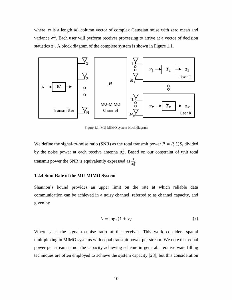
where 𝒏 is a length 𝑀𝑖 column vector of complex Gaussian noise with zero mean and

variance 𝜎𝑛2. Each user will perform receiver processing to arrive at a vector of decision

statistics 𝒛𝑖. A block diagram of the complete system is shown in Figure 1.1.

Figure 1.1: MU-MIMO system block diagram

We define the signal-to-noise ratio (SNR) as the total transmit power 𝑃 = 𝑃𝑠 ∑𝑆𝑖 divided

by the noise power at each receive antenna 𝜎𝑛2. Based on our constraint of unit total

transmit power the SNR is equivalently expressed as 1

𝜎𝑛2.

1.2.4 Sum-Rate of the MU-MIMO System

Shannon’s bound provides an upper limit on the rate at which reliable data

communication can be achieved in a noisy channel, referred to as channel capacity, and

given by

𝐶 = log2(1 + 𝛾) (7)

Where 𝛾 is the signal-to-noise ratio at the receiver. This work considers spatial

multiplexing in MIMO systems with equal transmit power per stream. We note that equal

power per stream is not the capacity achieving scheme in general. Iterative waterfilling

techniques are often employed to achieve the system capacity [28], but this consideration

11

is outside the scope of this work. We instead consider the sum-rate of the system. The

sum-rate of a SU-MIMO system employing spatial multiplexing is shown in equation 8.

𝑅 = ∑ 𝑙𝑜𝑔2(1 + 𝛾𝑚)

𝑆

𝑚=1

(8)

Where 𝛾𝑚 is the signal-to-interference-and-noise ratio (SINR) of the 𝑚𝑡ℎ stream,

assuming Gaussian interference. In this case the interference is caused by the transmitted

streams bleeding into one another, referred to as inter-stream-interference. Assuming the

𝑚𝑡ℎstream is precoded at the transmitter using 𝒘𝑚 and processed at the receiver using

𝒕𝑚, the SINR of the 𝑚𝑡ℎ stream at the output of the receiver is given by

𝛾𝑚 =

‖𝒕𝑚𝑯𝒘𝑚‖2

𝑀𝜎𝑛2 + ∑ ‖𝒕𝑚𝑯𝒘𝑛‖2𝑆

𝑛=1,𝑛≠𝑚

(9)

Where 𝒘𝑛 is the vector of precoding weights applied to the 𝑛 ≠ 𝑚𝑡ℎ stream and is

therefore a source of interference.

In a MU-MIMO system the sum-rate expression must include an additional summation

across all of the co-scheduled users along with the summation of their possibly unique

number of streams [13]. This is the expression which is used to calculate the sum-rate

throughout the rest of this work and is shown in equation 10.

𝑅 = ∑ ∑ 𝑙𝑜𝑔2(1 + 𝛾𝑖,𝑚)

𝑆𝑖

𝑚=1

𝐾

𝑖=1

(10)

The SINR for each stream must also consider the interference from co-scheduled users.

The SINR for the 𝑚𝑡ℎ stream of the 𝑖𝑡ℎ user is then

𝛾𝑖,𝑚 =

‖𝒕𝑚𝑯𝑖𝒘𝑖,𝑚‖2

𝑀𝑖𝜎𝑛2 + ∑ ‖𝒕𝑚𝑯𝑖𝒘𝑖,𝑛‖

2𝑆𝑛=1,𝑛≠𝑚 + ∑ ‖𝑻𝑚𝑯𝑖𝑾𝑘‖2𝐾

𝑘=1,𝑘≠𝑖

(11)

12

Analysis of MU-MIMO systems often limits users to a single stream each, in which case

the SINR for the 𝑖𝑡ℎ user is

𝛾𝑖 =

‖𝒕𝑚𝑯𝑖𝑾𝑖‖2

𝑀𝑖𝜎𝑛2 + ∑ ‖𝒕𝑚𝑯𝑖𝑾𝑘‖2𝐾

𝑘=1,𝑘≠𝑖

(12)

Chapter 2

13

Background: Conventional MU-MIMO

Techniques

Before extending analysis to incorporate practical considerations such as imperfect CSIT

and CSIR, antenna correlation, and/or time-varying channels, it’s important to develop a

firm understanding of the conventional MU-MIMO system concepts including precoding

techniques and receiver architectures in ideal conditions. This chapter reviews these

concepts as well as the particular algorithm of interest, referred to as the iterative signal-

to-leakage-and-noise ratio (iSLNR) algorithm which is expanded upon later in this work.

2.1 Receiver Architectures

Receivers can be classified in several ways; being either linear or non-linear and either

interference-aware or interference-unaware. A receiver is linear if it arrives at a set of

decision statistics by taking a linear transform of the received signal vector 𝒓. The

applied linear transform is represented by the matrix 𝑻, which has dimension 𝑆𝑖x𝑀𝑖, and

the length 𝑆𝑖 column vector of decision statistics 𝒛 is given by:

𝒛 = 𝑻 𝒓 (13)

Non-linear receivers on the other hand, do not apply linear weights, but perform some

non-linear operation to obtain the best estimate of the transmitted symbols. Examples of

non-linear receivers include Successive Interference Cancellation (SIC) receivers and

Maximum Likelihood (ML) receivers. This work considers linear receivers as they are

more commonly used in mobile devices where low-complexity is extremely important.

Interference suppression at the receiver can play an important role in reducing the effect of

multiuser interference. Naturally this capability requires the receiver to be interference-

aware, having some knowledge of composition of the interfering signals and/or estimates

of their statistical properties. There have been a number of papers showing the superiority

of interference-aware receivers such as the interference rejection combining (IRC) and

Max-Log-MAP receivers, over interference-unaware receivers such as the conventional

matched filter (MF) or minimum mean square error (MMSE) receivers [10,11]. Much of

14

the previous work has focused on the case where precoding is limited to a finite codebook

and a specific precoding matrix is chosen based on feedback from the receiver; a common

architecture in today’s wireless systems. In this case, interference-aware receivers

outperform interference-unware receivers due to the quantization of CSIT to a finite

codebook which creates significant multiuser interference. That being said, there has been

a great deal of effort to move away from the limitation of a finite codebook, possibly

exploiting the reciprocity of the wireless channel that exists in a TDD system for CSIT

acquisition. For example, release 10 of LTE-A defined Transmission Mode 9, which

enables transparent precoding [1]. Transparent precoding implies that the user requires no

knowledge of the precoding matrix employed at the base station, this is contrary to the

previous Transmission Modes in which the precoding matrix was signaled to the user to

enable demodulation. Transparent precoding enables the use of non-codebook-based

precoding schemes. The precoding will naturally be accounted for in the channel

estimation at the receiver. In this case the transmitter should ideally suppress the multiuser

interference sufficiently such that little benefit would be realized from an interference-

aware receiver. While this is true under ideal conditions, one of the results of this paper

shows that, as from quantization of CSIT to a finite codebook, imperfect CSIT will cause

non-trivial residual multiuser interference such that an interference-aware receiver will

provide significant performance gains compared to an interference-unaware receiver.

In the next sections we briefly review the conventional linear receiver types. Many of

these receiver types are applicable in both the SU-MIMO and MU-MIMO case. Of course

in the SU-MIMO case 𝑮𝑖 = 𝑮, but we include the subscript to be clear.

2.1.1 Matched Filter Receiver:

The matched filter (MF) receiver will de-rotate the received symbols to acquire their

intended phase. Since it does not apply any amplitude correction, this receiver type is

only applicable for phase modulated signals such as QPSK. The MF receiver weights are

given by

15

𝑻𝑀𝐹 = 𝑮𝑖∗ (14)

Note that the MF receiver is only applicable when 𝑮𝑖 is assumed to be diagonal. This

may indeed be true when precoding is employed at the transmitter so as to diagonalize

the channel, but is not true in general.

2.1.2 Zero Forcing Receiver:

The zero forcing (ZF) receiver will completely eliminate all inter-stream-interference

without considering the additive noise from the receiver. The weights used by the ZF

receiver are given by [14]:

𝑻𝑍𝐹 = (𝑮𝑖∗ 𝑮𝑖 )

−1𝑮𝑖∗ (15)

When the channel magnitude is small the ZF receiver will apply a large gain. This large

gain is equally applied to the receiver noise which leads to degraded performance. This

effect is known as noise-enhancement.

2.1.3 Minimum Mean Squared Error Receiver:

The minimum mean square error (MMSE) receiver minimizes the total error power that

results from inter-stream-interference and noise. This effectively mitigates the issue of

noise-enhancement that can occur with the ZF receiver. The MMSE weights are

calculated as [14]

𝑻𝑀𝑀𝑆𝐸 = (𝑮𝑖∗ 𝑮𝑖 + 𝜎𝑛

2 𝑰)−1𝑮𝑖∗ (16)

2.1.4 Interference Rejection Combining Receiver:

In a system with multiple users there may be additional sources of interference at each

receiver due to signals intended for other users. The ZF and MMSE receivers are limited

in that they do not make use of any sort of knowledge of the interfering signals to

mitigate their impact. The interference rejection combining (IRC) receiver on the other

hand is able to suppress the multiuser-interference by utilizing knowledge the

interference plus noise covariance matrix 𝑹𝑛. The IRC weights are found from [14]

16

𝑻𝐼𝑅𝐶 = (𝑮𝑖∗𝑹𝑛

−1𝑮𝑖)−1𝑮𝑖

∗𝑹𝑛−1 (17)

The interference plus noise covariance matrix is given by

𝑹𝑛 = 𝐸{𝜼𝜼∗}, 𝜼 = 𝑮𝑛𝒔𝑛 + 𝒏 (18)

where 𝒔𝑛 is the vector of the interfering symbols, 𝑮𝑛 is the equivalent channel for the

interfering signals to the 𝑖𝑡ℎ user given by 𝑮𝑛 = 𝑯𝑖𝑾𝑛 where 𝑾𝑛 is the precoding

matrix associated with all interfering streams, and 𝒏 is a complex Gaussian noise vector

with variance 𝜎𝑛2. These terms are written out explicitly below.

𝒔𝑛 =

[

𝒔1

⋮𝒔𝒊−𝟏𝒔𝒊+𝟏

⋮𝒔𝐾 ]

𝑾𝑛 = [𝑾1, … ,𝑾𝑖−1,𝑾𝑖+1, … ,𝑾𝐾]

𝑮𝑛 = 𝑯𝑖𝑾𝑛 (19)

Assuming the elements of 𝒔𝑛 have unit average power and a uniformly distributed phase,

𝑹𝑛 can be equivalently expressed

𝑹𝑛 = 𝑮𝑛𝑮𝑛∗ + 𝜎𝑛

2𝑰 (20)

2.2 Conventional MU-MIMO Precoding

This section discusses the conventional MU-MIMO linear precoding techniques and the

tradeoffs between them.

17

2.2.1 Complete Channel Diagonalization

Since it is assumed that the channel is known at the transmitter, the most obvious option

is to design the precoding matrix to completely invert the channel, 𝑾 = 𝑯−1 which

would yield a received vector

𝒓 = 𝑯𝑯−1𝒔 + 𝒏 = 𝒔 + 𝒏 (21)

The issue with this approach arises from the limitation of finite transmit power. Because

of this limitation, the precoding matrix must be scaled by some scalar 𝛽 such that

‖𝛽𝑯−1‖2 = 𝑃 (22)

In our analysis we’ve assumed that 𝑃 = 1, so 𝛽 =1

‖𝑯−1‖. Substituting the precoding

matrix into equation 6 gives us

𝒓 = 𝑯𝛽𝑯−1𝒔 + 𝒏

𝒓 =

1

‖𝑯−1‖𝒔 + 𝒏 (23)

Since the wireless channel will exhibit some fading characteristics, there will surely be

instances of deep fades where ‖𝑯‖ ≪ 1 which will imply ‖𝑯−1‖ ≫ 1, leading to

reduced signal power at the receiver and poor performance. This result is analogous to

the noise enhancement experienced at a receiver using ZF processing.

Note that in the case of non-square channel matrices this approach uses the pseudo-

inverse i.e. 𝑾 ∝ (𝑯∗𝑯)−𝟏𝑯∗.

2.2.2 Block-Diagonal Zero-Forcing

Block-Diagonal Zero-Forcing precoding recognizes that there is no need for the

transmitter to separate streams intended for a common user. Doing so is often a redundant

operation because the receiver will be able to sufficiently separate the streams later with

high probability. Instead, it is sufficient to force all multiuser-interference terms to zero

18

by ensuring that the equivalent channel matrix is block diagonal. To remind the reader,

the equivalent channel is given by

𝑮 =

𝑮11 … 𝑮1𝐾

⋮ ⋱ ⋮𝑮𝐾1 … 𝑮𝐾𝐾

(24)

Where 𝐺𝑖𝑗 is the equivalent channel from the 𝑗𝑡ℎ user’s data stream(s) to the 𝑖𝑡ℎ user’s

receive antenna(s). The multiuser-interference terms are therefore 𝑮𝑖𝑗∀𝑖 ≠ 𝑗. So by

forcing all multi-user interference terms to zero the equivalent channel will be of the form

𝑮 =

𝑮11 … 𝟎⋮ ⋱ ⋮𝟎 … 𝑮𝐾𝐾

(25)

which is block-diagonal. Clearly for this to be true, 𝑾𝑖 must be in the null-space of 𝑯𝑗

for all 𝑖 ≠ 𝑗. The advantage of this method is that it is less restrictive than complete

diagonalization of the channel, so the average SNR at the receiver will be improved. Of

course, when 𝑀𝑖 = 1 ∀ 𝑖, this method simplifies to complete channel diagonalization.

Once the nullspace constraint has been met, the problem has effectively been

decomposed into several SU-MIMO sub problems for which traditional SU-MIMO

precoding solutions can be used. The precoding matrix for the 𝑖𝑡ℎ user is then given by

𝑾𝑖 = 𝒀𝑖𝑿𝑖 (26)

Where 𝒀𝑖 is chosen such that 𝑯𝑗𝒀𝑖 = 𝟎 ∀ 𝑗 ≠ 𝑖, and 𝑿𝑖 is chosen to maximize the SNR

for the 𝑖𝑡ℎ user using traditional SU-MIMO techniques such as eigen-beamforming. The

SNR for the 𝑖𝑡ℎ user is given

𝑆𝑁𝑅𝑖 =

‖𝑯𝑖𝒀𝑖𝑿𝑖‖2

𝑀𝑖𝜎𝑛2

(27)

19

So 𝑿𝑖 must be chosen to maximize ‖𝑯𝑖𝒀𝑖𝑿𝑖‖2 = 𝑇𝑟[𝑿𝑖

∗𝒀𝑖∗𝑯𝑖

∗𝑯𝑖𝒀𝑖𝑿𝑖] given 𝑯𝑖 and 𝒀𝑖.

This can be accomplished using eigendecomposition from which we know there exists a

𝑸 and Λ such that

𝑸∗𝒀𝑖∗𝑯𝑖

∗𝑯𝑖𝒀𝑖𝑸 = Λ (28)

where the columns of 𝑸 are the right eigenvectors of 𝒀𝑖∗𝑯𝑖

∗𝑯𝑖𝒀𝑖, and 𝚲 is a diagonal

matrix with elements in descending order i.e. 𝜆1 ≥ ⋯𝜆𝑀𝑖≥ 0, and where 𝜆𝑖 is the

eigenvalue associated with eigenvector in the 𝑖𝑡ℎ column of 𝑸. To maximize the

expression in equation 28 and maintaining separable streams the precoding matrix 𝑾𝑖

must be constructed using the 𝑆𝑖 eigenvectors associated with the largest eigenvalues i.e.

the 𝑆𝑖 left-most columns of 𝑸.

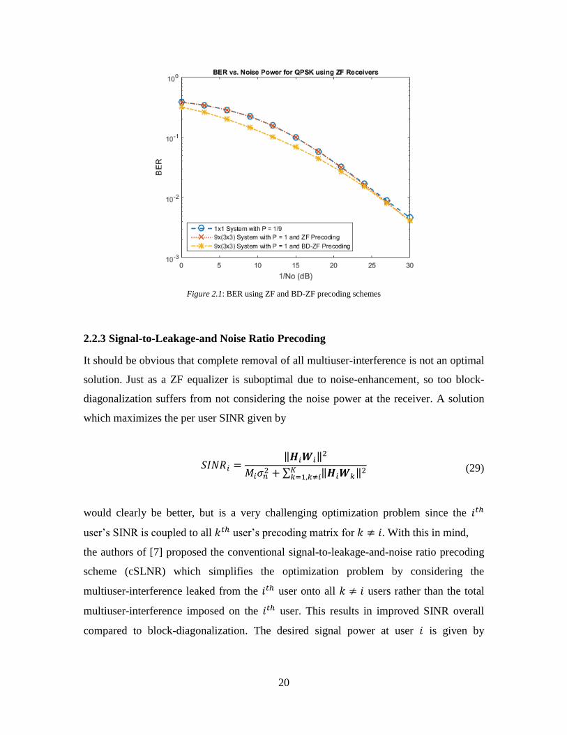
Figure 2.1 shows a comparison of the bit error rates using complete channel

diagonalization and block-diagonalization in a 9x(3x3) system with 3 streams per user.

Block-diagonalization clearly offers improved performance in the lower SNR regime by

reducing noise enhancement compared to complete channel diagonalization as described

earlier. As a baseline we’ve also included the error rate for a 1x1 system where the

transmit power is normalized to be equal to the per stream transmit power of the 9x(3x3)

system. In this case we observe that the performance is identical to the MU-MIMO

system with ZF precoding.

20

Figure 2.1: BER using ZF and BD-ZF precoding schemes

2.2.3 Signal-to-Leakage-and Noise Ratio Precoding

It should be obvious that complete removal of all multiuser-interference is not an optimal

solution. Just as a ZF equalizer is suboptimal due to noise-enhancement, so too block-

diagonalization suffers from not considering the noise power at the receiver. A solution

which maximizes the per user SINR given by

𝑆𝐼𝑁𝑅𝑖 =

‖𝑯𝑖𝑾𝑖‖2

𝑀𝑖𝜎𝑛2 + ∑ ‖𝑯𝑖𝑾𝑘‖2𝐾

𝑘=1,𝑘≠𝑖

(29)

would clearly be better, but is a very challenging optimization problem since the 𝑖𝑡ℎ

user’s SINR is coupled to all 𝑘𝑡ℎ user’s precoding matrix for 𝑘 ≠ 𝑖. With this in mind,

the authors of [7] proposed the conventional signal-to-leakage-and-noise ratio precoding

scheme (cSLNR) which simplifies the optimization problem by considering the

multiuser-interference leaked from the 𝑖𝑡ℎ user onto all 𝑘 ≠ 𝑖 users rather than the total

multiuser-interference imposed on the 𝑖𝑡ℎ user. This results in improved SINR overall

compared to block-diagonalization. The desired signal power at user 𝑖 is given by

21

‖𝑯𝑖𝑾𝑖‖2 and the MUI imposed on all other users by this precoding is then

∑ ‖𝑯𝑘𝑾𝑖‖2𝐾

𝑘=1,𝑘≠𝑖 . So the SLNR is given by:

𝑆𝐿𝑁𝑅 =


𝑀𝑖𝜎𝑛2 + ‖�̃�𝑖𝑾𝑖‖

2 (30)

Where �̃�𝑖 = [𝑯1 …𝑯𝑖−1𝑯𝑖+1 …𝑯𝐾]𝑇 is the so called ‘leakage channel’. Note that the

SLNR is merely a metric used to approximate the problem of maximizing SINR. It is the

SINR at each user that ultimately determines their performance and therefore that of the

system as a whole. Expanding equation 30 gives

𝑆𝐿𝑁𝑅 =

𝑇𝑟[𝑾𝑖∗𝑯𝑖

∗𝑯𝑖𝑾𝑖]

𝑀𝑖𝜎𝑛2𝑰 + 𝑇𝑟[𝑾𝑖

∗�̃�𝑖∗�̃�𝑖𝑾𝑖]

(31)

Noting that 𝑇𝑟[𝑾𝑖∗𝑾𝑖] = 𝑆𝑖𝑃𝑠 this can be equivalently expressed

=

𝑇𝑟[𝑾𝑖∗𝑯𝑖

∗𝑯𝑖𝑾𝑖]

𝑇𝑟 [𝑾𝑖∗ (�̃�𝑖

∗�̃�𝑖 +𝑀𝑖

𝑆𝑖𝑃𝑠𝜎𝑛

2𝑰)𝑾𝑖] (32)

Equation 32 is of the familiar Rayleigh Quotient form, 𝑯𝑖∗𝑯𝑖 being Hermitian and

𝑀𝑖


2𝑰 + �̃�𝑖∗�̃�𝑖 being Hermitian and positive-definite. It can therefore be expressed as

𝑸∗𝑯𝑖∗𝑯𝑖𝑸 = 𝚲

𝑸∗ (

𝑀𝑖


2𝑰 + �̃�𝑖∗�̃�𝑖)𝑸 = 𝑰 (33)

Where the columns of 𝑸 are the right generalized eigenvectors of the pair

{𝑯𝑖∗𝑯𝑖,

𝑀𝑖


2𝑰 + �̃�𝑖∗�̃�𝑖}, and 𝚲 is a diagonal matrix with elements 𝜆1 ≥ ⋯𝜆𝑀 ≥ 0,

where 𝜆𝑖 is the eigenvalue associated with eigenvector in the 𝑖𝑡ℎ column of 𝑸. For a

single stream per user the SLNR is then maximized by selecting 𝑾𝑖 to be the eigenvector

22

associated with the largest eigenvalue e.g. the left-most column of 𝑸. Through the rest of

the paper we see this same eigendecomposition problem many times with minor

differences. In each case we apply the same approach and write the solution compactly in

the following manner to ease notation.

𝑾𝑖 ∝ 𝑚𝑎𝑥 𝑒𝑖𝑔𝑒𝑛𝑣𝑒𝑐𝑡𝑜𝑟 ((�̃�𝑖

∗�̃�𝑖 +𝑀𝑖


2𝑰)−1

𝑯𝑖∗𝑯𝑖) (34)

The extension to multiple streams is quite natural. In order for the streams to be

decoupled at the 𝑖𝑡ℎ user we require that 𝑾𝑖∗𝑯𝑖

∗𝑯𝑖𝑾𝑖 is diagonal. For a user with 𝑆𝑖

streams, the columns of 𝑾𝑖 should therefore be proportional to the eigenvectors

corresponding to the 𝑆𝑖 largest eigenvalues of the pair {𝑯𝑖∗𝑯𝑖,

𝑀𝑖


2𝑰 + �̃�𝑖∗�̃�𝑖} which we

write as

𝑾𝑖 ∝ 𝑆𝑖 𝑚𝑎𝑥 𝑒𝑖𝑔𝑒𝑛𝑣𝑒𝑐𝑡𝑜𝑟𝑠 ((�̃�𝑖

∗�̃�𝑖 +𝑀𝑖


2𝑰)−1

𝑯𝑖∗𝑯𝑖) (35)

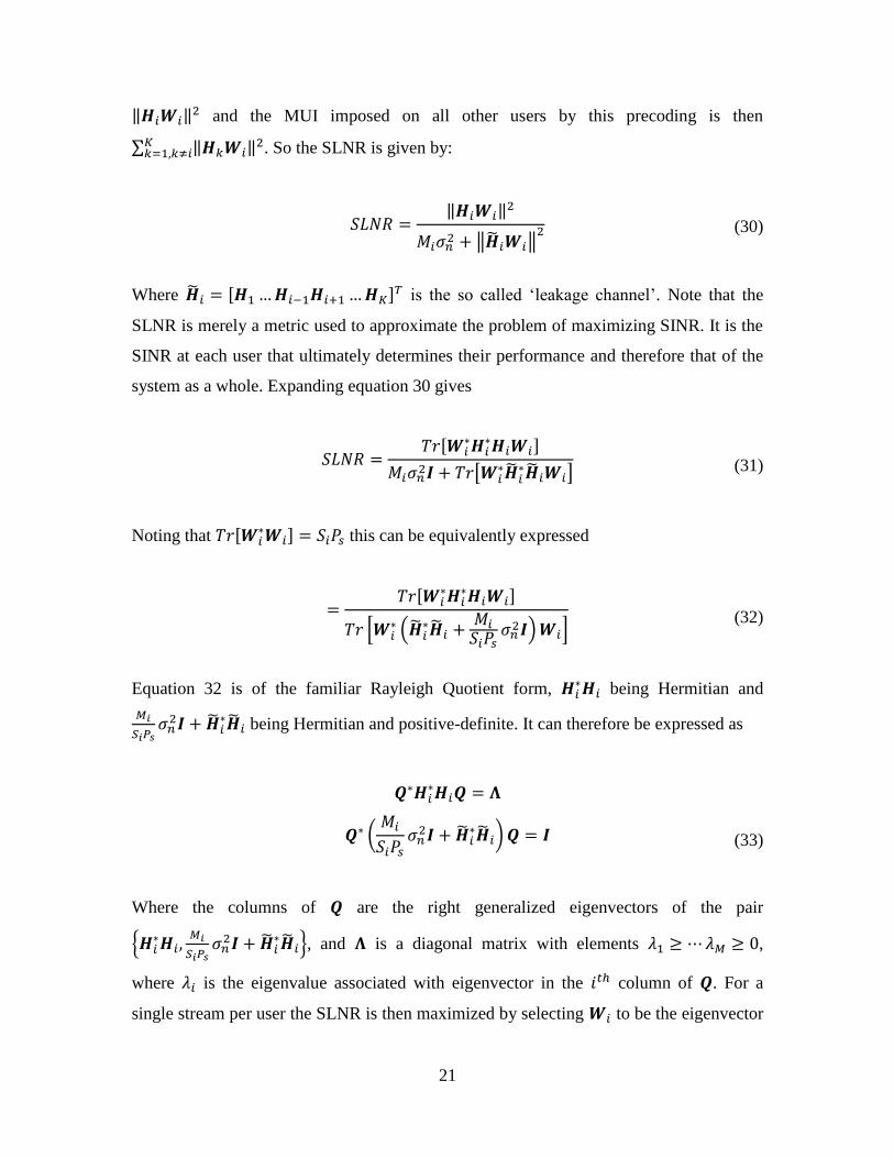
Figure 2.2 shows a comparison of error rates between the SLNR and BD-ZF precoding

schemes for a 9x(3x3) system with three streams per user. You can see that SLNR

precoding provides better performance since it accounts for noise at the receiver, whereas

BD-ZF precoding does not.

23

Figure 2.2: BER using BD-ZF and SLNR precoding schemes

SLNR precoding also has the added benefit that it can be applied in systems where the

number of transmit antennas is less than the sum of receive antennas. This is not true for

the ZF schemes which require sufficient degrees of freedom to completely remove the

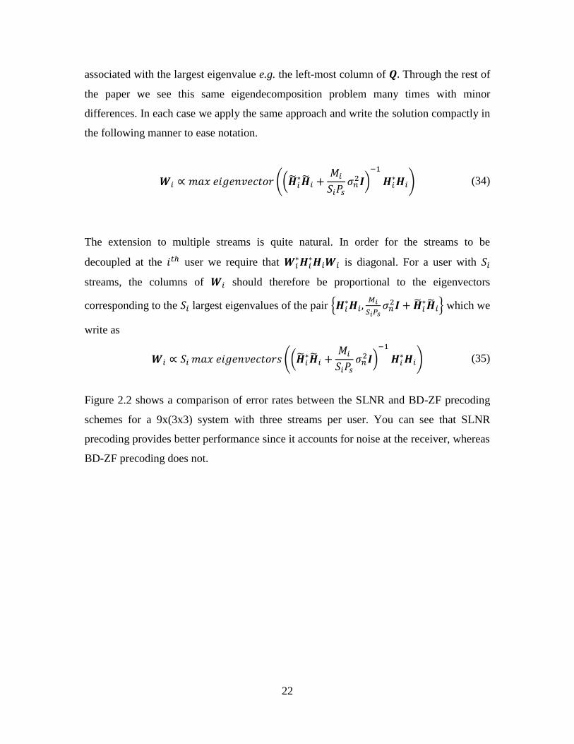
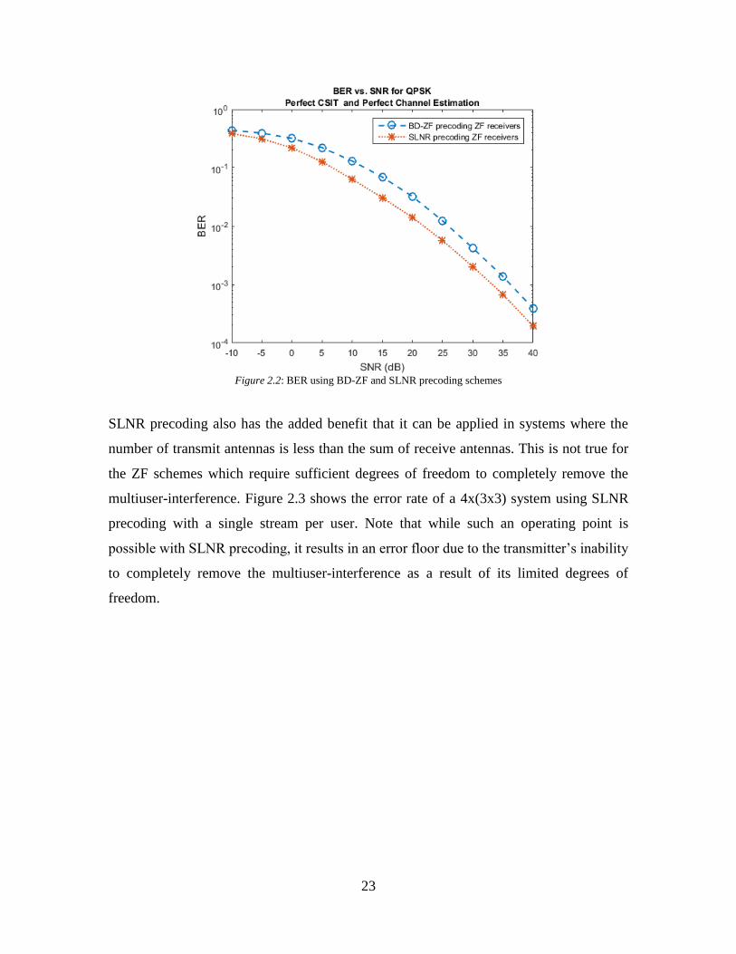
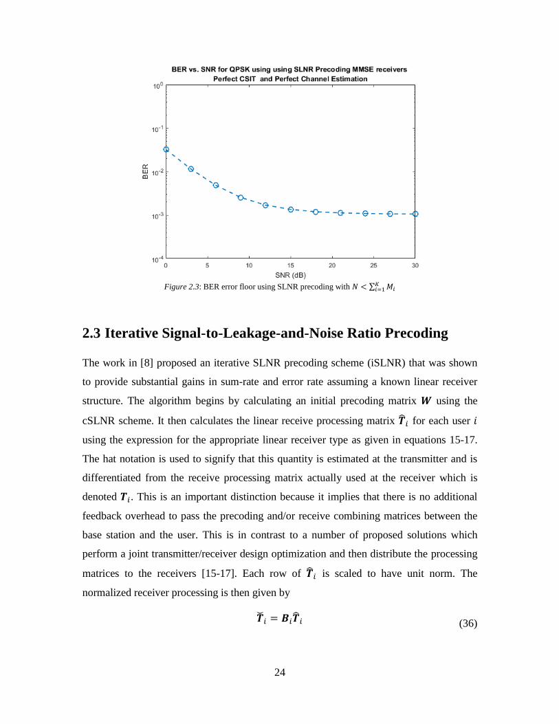
multiuser-interference. Figure 2.3 shows the error rate of a 4x(3x3) system using SLNR

precoding with a single stream per user. Note that while such an operating point is

possible with SLNR precoding, it results in an error floor due to the transmitter’s inability

to completely remove the multiuser-interference as a result of its limited degrees of

freedom.

24

Figure 2.3: BER error floor using SLNR precoding with 𝑁 < ∑ 𝑀𝑖

𝐾𝑖=1

2.3 Iterative Signal-to-Leakage-and-Noise Ratio Precoding

The work in [8] proposed an iterative SLNR precoding scheme (iSLNR) that was shown

to provide substantial gains in sum-rate and error rate assuming a known linear receiver

structure. The algorithm begins by calculating an initial precoding matrix 𝑾 using the

cSLNR scheme. It then calculates the linear receive processing matrix �̂�𝑖 for each user 𝑖

using the expression for the appropriate linear receiver type as given in equations 15-17.

The hat notation is used to signify that this quantity is estimated at the transmitter and is

differentiated from the receive processing matrix actually used at the receiver which is

denoted 𝑻𝑖. This is an important distinction because it implies that there is no additional

feedback overhead to pass the precoding and/or receive combining matrices between the

base station and the user. This is in contrast to a number of proposed solutions which

perform a joint transmitter/receiver design optimization and then distribute the processing

matrices to the receivers [15-17]. Each row of �̂�𝑖 is scaled to have unit norm. The

normalized receiver processing is then given by

�̌�𝑖 = 𝑩𝑖�̂�𝑖 (36)

25

Where 𝑩𝑖 is a diagonal matrix with elements 𝑏𝑗𝑗 =1

‖𝒕𝑖,𝑗‖, with �̂�𝑖,𝑗 being the 𝑗𝑡ℎ row of �̂�𝑖.

Using the normalized receiver processing calculated at the transmitter, the algorithm then

defines an effective channel �̌�𝑖 for each user 𝑖, which is given by

�̌�𝑖 ≜ [�̌�𝑖

𝟎]𝑯𝑖 (37)

The zero rows are included to maintain the dimension of �̌�𝑖 as being equal to the

dimension of 𝑯𝑖. This is necessary when 𝑆𝑖 < 𝑀𝑖, which is a requirement for the iSLNR

algorithm to provide performance improvement to the system. When 𝑆𝑖 = 𝑀𝑖, the iSLNR

algorithm collapses to the cSLNR scheme.

With the effective channel for each user at hand, the algorithm then recalculates the

precoding matrices using a modified definition of the SLNR metric (mSLNR) which relies

on the effective leakage channel, defined as

�̅�𝑖 ≜ [�̌�1, … , �̌�𝑖−1, �̌�𝑖+1, … , �̌�𝐾]𝑇 (38)

The modified SLNR metric is then

𝑚𝑆𝐿𝑁𝑅 =


𝑆𝑖𝜎𝑛2 + ‖�̅�𝑖𝑾𝑖‖2

(39)

Note that the noise power is scaled by the number of streams 𝑆𝑖 rather than the number of

antennas 𝑀𝑖 as in the cSLNR metric. This is to ensure that the noise and leakage powers

are considered equally. In this mSLNR metric the leakage power is considered at the

output of the normalized receiver processing. The total noise at this point will therefore be

proportional to the number of streams rather than the number of antennas. We further note

the importance of normalizing each row of the receiver processing matrix �̂�, which is

necessary to maintain proportionality between the noise and leakage.

26

The solution for the 𝑾𝑖 which will maximize the expression given in equation 39 is found

using eigendecomposition as in the derivation of eqs. 34 and 35 and is given by

𝑾𝑖 ∝ 𝑆𝑖 max 𝑒𝑖𝑔𝑒𝑛𝑣𝑒𝑐𝑡𝑜𝑟𝑠 ((�̅�𝑖

∗�̅�𝑖 +1

𝑃𝑠

𝜎𝑛2𝑰)

−1

𝑯𝑖∗𝑯𝑖)

(40)

This updated precoding matrix is then used to recalculate the normalized receiver

processing matrices �̌�𝒊 and update the effective leakage channels �̅�𝑖. The algorithm

continues to alternate between calculating the precoding matrix and updating the

effective leakage channels for however many iterations are to be performed, denoted

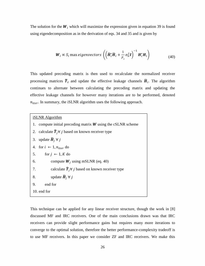
𝑛𝑖𝑡𝑒𝑟. In summary, the iSLNR algorithm uses the following approach.

This technique can be applied for any linear receiver structure, though the work in [8]

discussed MF and IRC receivers. One of the main conclusions drawn was that IRC

receivers can provide slight performance gains but requires many more iterations to

converge to the optimal solution, therefore the better performance-complexity tradeoff is

to use MF receivers. In this paper we consider ZF and IRC receivers. We make this

iSLNR Algorithm

1. compute initial precoding matrix 𝑾 using the cSLNR scheme

2. calculate �̂�𝑗∀ 𝑗 based on known receiver type

3. update �̌�𝑗 ∀ 𝑗

4. for 𝑖 ← 1, 𝑛𝑖𝑡𝑒𝑟 do

5. for 𝑗 ← 1, 𝐾 do

6. compute 𝑾𝑗 using mSLNR (eq. 40)

7. calculate �̂�𝑗∀ 𝑗 based on known receiver type

8. update �̌�𝑗 ∀ 𝑗

9. end for

10. end for

27

distinction so that we can investigate error rates using higher order modulations, where

the MF receiver would not be applicable. As stated previously the MF receiver only

corrects the phase rotation of the received symbol, not its amplitude. This means that the

MF receiver cannot be used with amplitude modulated signals i.e. quadrature-amplitude-

modulation (QAM). The ZF and IRC receiver weights were provided in equations 15 and

17.

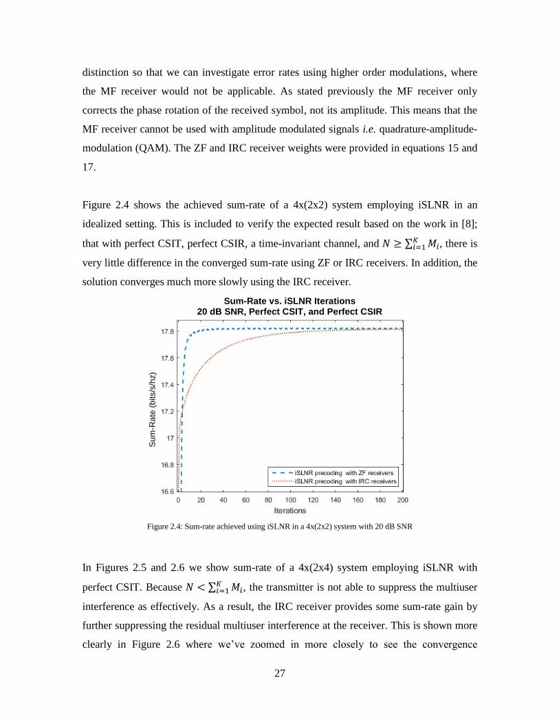
Figure 2.4 shows the achieved sum-rate of a 4x(2x2) system employing iSLNR in an

idealized setting. This is included to verify the expected result based on the work in [8];

that with perfect CSIT, perfect CSIR, a time-invariant channel, and 𝑁 ≥ ∑ 𝑀𝑖𝐾𝑖=1 , there is

very little difference in the converged sum-rate using ZF or IRC receivers. In addition, the

solution converges much more slowly using the IRC receiver.

Figure 2.4: Sum-rate achieved using iSLNR in a 4x(2x2) system with 20 dB SNR

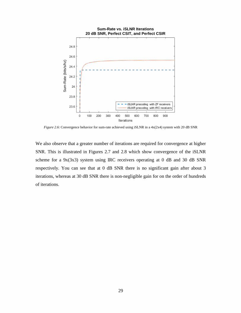
In Figures 2.5 and 2.6 we show sum-rate of a 4x(2x4) system employing iSLNR with

perfect CSIT. Because 𝑁 < ∑ 𝑀𝑖𝐾𝑖=1 , the transmitter is not able to suppress the multiuser

interference as effectively. As a result, the IRC receiver provides some sum-rate gain by

further suppressing the residual multiuser interference at the receiver. This is shown more

clearly in Figure 2.6 where we’ve zoomed in more closely to see the convergence

Sum-Rate vs. iSLNR Iterations 20 dB SNR, Perfect CSIT, and Perfect CSIR

Su

m-R

ate

(b

its/s

/hz)

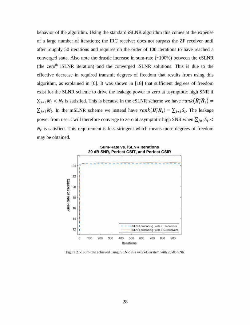
28

behavior of the algorithm. Using the standard iSLNR algorithm this comes at the expense

of a large number of iterations; the IRC receiver does not surpass the ZF receiver until

after roughly 50 iterations and requires on the order of 100 iterations to have reached a

converged state. Also note the drastic increase in sum-rate (~100%) between the cSLNR

(the zeroth iSLNR iteration) and the converged iSLNR solutions. This is due to the

effective decrease in required transmit degrees of freedom that results from using this

algorithm, as explained in [8]. It was shown in [18] that sufficient degrees of freedom

exist for the SLNR scheme to drive the leakage power to zero at asymptotic high SNR if

∑ 𝑀𝑖𝑗≠𝑖 < 𝑁𝑡 is satisfied. This is because in the cSLNR scheme we have 𝑟𝑎𝑛𝑘(�̃�𝑖∗�̃�𝑖) =

∑ 𝑀𝑖𝑗≠𝑖 . In the mSLNR scheme we instead have 𝑟𝑎𝑛𝑘(�̅�𝑖∗�̅�𝑖) = ∑ 𝑆𝑖𝑗≠𝑖 . The leakage

power from user 𝑖 will therefore converge to zero at asymptotic high SNR when ∑ 𝑆𝑖𝑗≠𝑖 <

𝑁𝑡 is satisfied. This requirement is less stringent which means more degrees of freedom

may be obtained.

Figure 2.5: Sum-rate achieved using iSLNR in a 4x(2x4) system with 20 dB SNR


Su

m-R

ate

(b

its/s

/hz)

29

Figure 2.6: Convergence behavior for sum-rate achieved using iSLNR in a 4x(2x4) system with 20 dB SNR

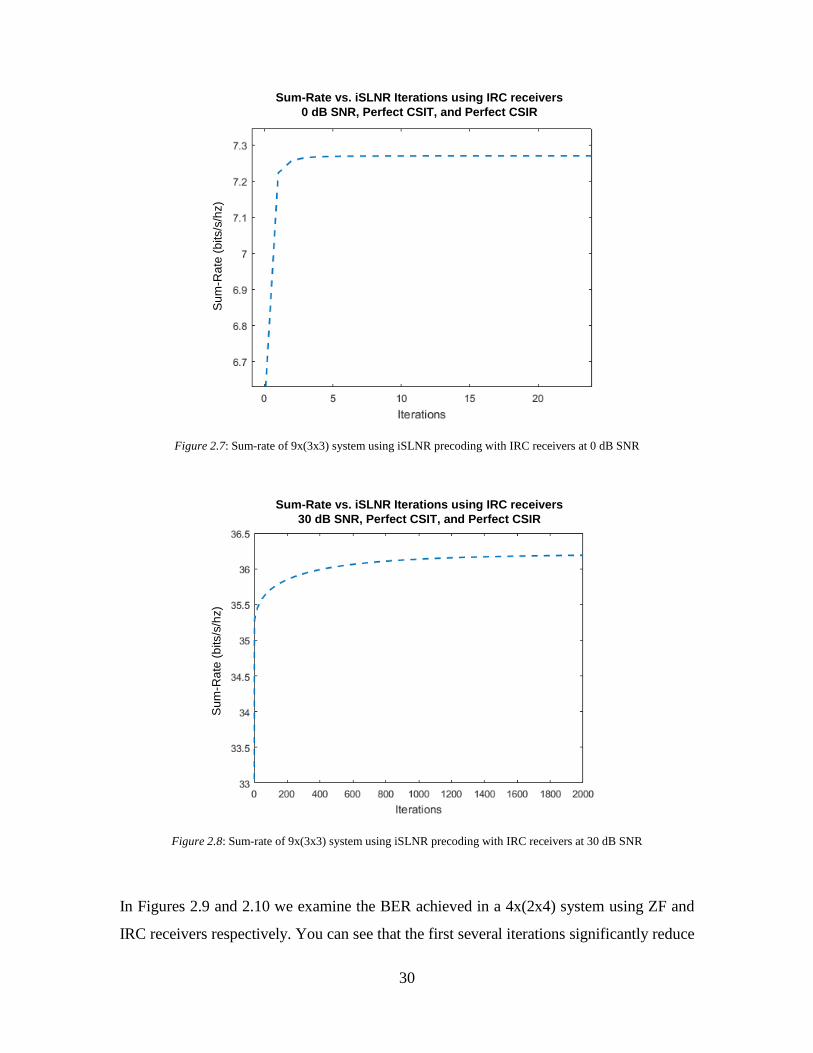
We also observe that a greater number of iterations are required for convergence at higher

SNR. This is illustrated in Figures 2.7 and 2.8 which show convergence of the iSLNR

scheme for a 9x(3x3) system using IRC receivers operating at 0 dB and 30 dB SNR

respectively. You can see that at 0 dB SNR there is no significant gain after about 3

iterations, whereas at 30 dB SNR there is non-negligible gain for on the order of hundreds

of iterations.


Su

m-R

ate

(b

its/s

/hz)

30

Figure 2.7: Sum-rate of 9x(3x3) system using iSLNR precoding with IRC receivers at 0 dB SNR

Figure 2.8: Sum-rate of 9x(3x3) system using iSLNR precoding with IRC receivers at 30 dB SNR

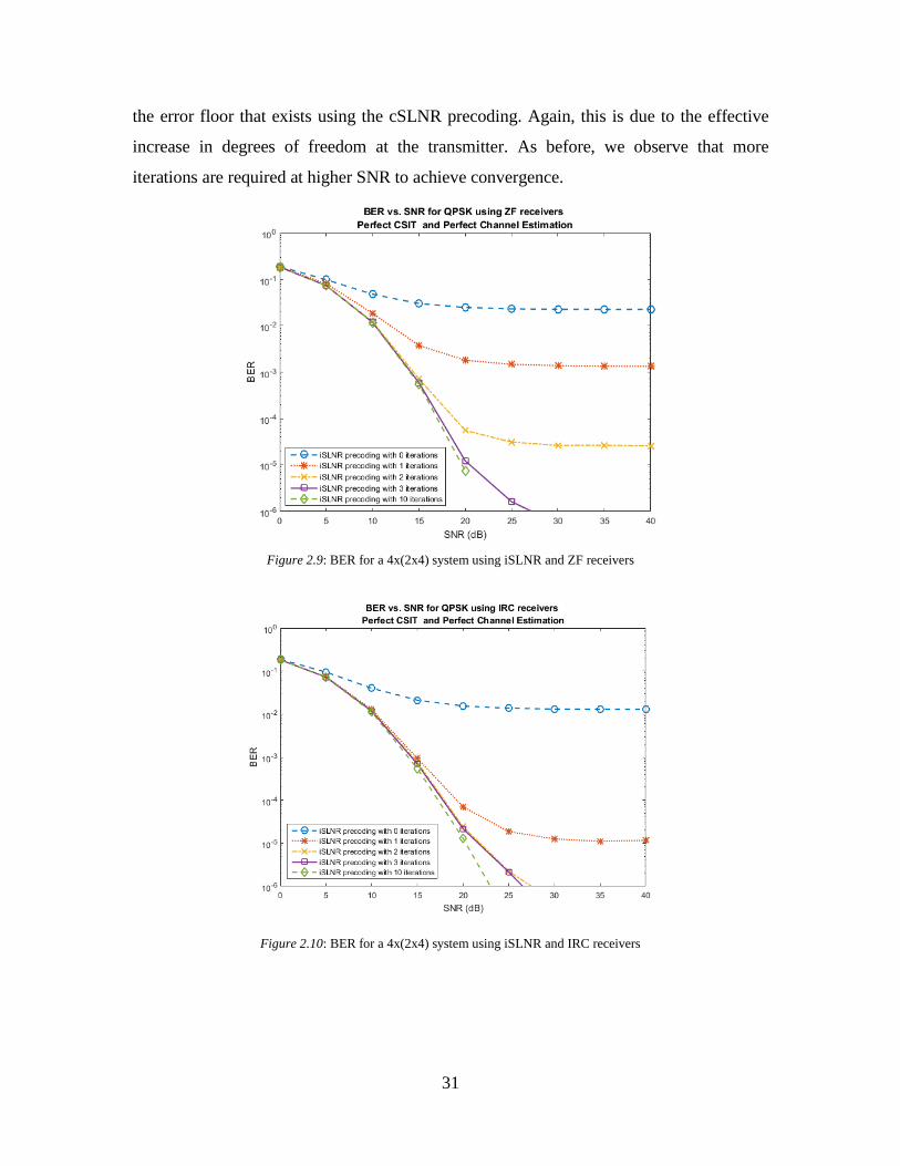
In Figures 2.9 and 2.10 we examine the BER achieved in a 4x(2x4) system using ZF and

IRC receivers respectively. You can see that the first several iterations significantly reduce

Sum-Rate vs. iSLNR Iterations using IRC receivers

0 dB SNR, Perfect CSIT, and Perfect CSIR

Su

m-R

ate

(b

its/s

/hz)



Su

m-R

ate

(b

its/s

/hz)

31

the error floor that exists using the cSLNR precoding. Again, this is due to the effective

increase in degrees of freedom at the transmitter. As before, we observe that more

iterations are required at higher SNR to achieve convergence.

Figure 2.9: BER for a 4x(2x4) system using iSLNR and ZF receivers

Figure 2.10: BER for a 4x(2x4) system using iSLNR and IRC receivers

32

2.4 Chapter Summary

In this chapter we reviewed the conventional MU-MIMO concepts including receiver

structures and precoding techniques. We explained the motivation to introduce the BD-

ZF scheme rather than the complete channel diagonalization of the ZF scheme and

showed the error rate performance gain achieved. We further explained how SLNR is a

useful approximation for SINR as it captures the figures of merit without the coupling

issue that exists when attempting to directly maximize SINR. The error rate performance

of SLNR precoding was compared to BD-ZF precoding and shown to be superior.

Finally, we reviewed the iSLNR precoding algorithm which iteratively maximizes a

modified definition of the SLNR metric wherein the leakage channel is considered at the

output of the receiver. This approach was shown to provide significant gains in error rate

and sum-rate, and to reduce the required degrees of freedom at the transmitter. All of this

analysis was performed in an ideal scenario. In the next chapters we’ll investigate the

impact of several practical impairments on system performance and ways to mitigate

them.

33

Chapter 3

Imperfect Channel State Information

In the previous chapter we reviewed several approaches to calculating the precoding

matrices of a MU-MIMO system and demonstrated the performance achieved using these

techniques under ideal conditions. For a practical system however, we must consider the

presence of non-idealities if we are to achieve the best possible system performance. Both

the transmit and receive techniques discussed require knowledge of the channel and are

negatively impacted when that knowledge is imperfect. There have been a number of

papers written describing methods to deal with imperfect channel state information at the

transmitter (CSIT) in the aforementioned precoding techniques [19-22]. No such work

exists specifically for the iSLNR algorithm however, which proved to be a very effective

precoding scheme for MU-MIMO systems. It is therefore the ultimate goal of this chapter

to investigate how this algorithm should be designed with imperfect CSIT. We also note

that the iSLNR algorithm relies on knowledge of the receiver processing to provide gain

to the system. In practice the receivers will have imperfect channel state information

which will impact their processing, so we must also investigate the performance of the

iSLNR algorithm with imperfect CSIR.

Before directly approaching the iSLNR algorithm with imperfect CSIT, we must make

sure that we fully understand the cSLNR precoding scheme with imperfect CSIT. This

chapter is structured into four sections. The first section investigates cSLNR precoding

with imperfect CSIT, the second section investigates the iSLNR algorithm with imperfect

CSIT, the third section investigates iSLNR precoding with imperfect CSIR, and finally

the last section summarizes our conclusions.

3.1 SLNR Precoding Considering CSIT Error

In practice the CSIT used for precoding will have some associated error with respect to

the true MIMO channel 𝑯, which will degrade system performance. The motivation of

the following work is therefore to minimize these degradations. We model the CSIT error

34

as the matrix 𝚪, whose elements are independent and identically distributed complex

Gaussian random variables with zero mean and variance 𝜎𝑐2. When a system is said to

have 𝑥 dB CSIT, the implication is that 𝑥 = 10𝑙𝑜𝑔10 (1

𝜎𝑐2) since the variance of each

element of the MIMO channel is unity. In general the dimensions of 𝚪 should be inferred

from context as it is used in several expressions e.g., for a particular user’s channel or for

leakage channels. Hereafter we denote quantities that are estimated at the transmitter

using (∙)̂, so the estimates available at the transmitter for the 𝑖𝑡ℎ user’s channel and

leakage channel are given by

�̂�𝑖 = 𝑯𝑖 + 𝚪i (41)

�̂̃�𝑖 = �̃�𝑖 + �̃�𝑖 (42)

In the following analysis it is assumed that the transmitter has perfect knowledge of the

second order statistics of the CSIT error, 𝜎𝑐2.

3.1.1 Revisiting the Existing SLNR Solution

In [7] the authors derived the solution for the precoding matrix which will maximize the

SLNR with imperfect CSIT using the same error model as we’ve described above. They

began from the SLNR expression conditioned on the 𝑖𝑡ℎ user channel estimate �̂�𝑖 and the

leakage channel estimate �̂̃�𝑖 at the transmitter.

𝑆𝐿𝑁𝑅 =

𝐸{𝑇𝑟[𝑾𝑖∗𝑯𝑖

∗𝑯𝑖𝑾𝑖] | �̂�𝑖}

𝑀𝑖𝜎𝑛2 + 𝐸 {𝑇𝑟[𝑾𝑖

∗�̃�𝑖∗�̃�𝑖𝑾𝑖] | �̂̃�𝑖}

(43)

The authors then used equations 41 and 42 to substitute �̂�𝑖 − 𝚪𝑖 for 𝑯 and �̂̃�𝑖 − �̃�𝑖 for �̃�𝑖.

=

𝐸{𝑇𝑟[𝑾𝑖∗(�̂�𝑖 − 𝚪𝑖 )

∗(�̂�𝑖 − 𝚪𝑖 )𝑾𝑖] | �̂�𝑖}

𝑀𝑖𝜎𝑛2 + 𝐸 {𝑇𝑟 [𝑾𝑖

∗ (�̂̃�𝑖 − �̃�𝑖)∗

(�̂̃�𝑖 − �̃�𝑖)𝑾𝑖] | �̂̃�𝑖}

(44)

35

Expanding this expression they arrived at the following solution to maximize the SLNR

in the presence of CSIT error (we avoid going through this derivation as we will shortly

show a very similar one).

𝑾𝑖 ∝ 𝑆𝑖 max 𝑒𝑖𝑔𝑒𝑛𝑣𝑒𝑐𝑡𝑜𝑟𝑠 𝑜𝑓

(

(�̂̃�𝑖∗�̂̃�𝑖 + ( ∑ 𝑀𝑗

𝐾

𝑗=1,𝑗≠𝑖

𝜎𝑐2 +

𝑀𝑖


2) 𝑰)

−1

(�̂�𝑖∗�̂�𝑖 + 𝑀𝑖𝜎𝑐

2𝑰)

)

(45)

The issue we see in this derivation is that the distribution of 𝑯𝑖 conditioned on �̂�𝑖 has

been represented as �̂�𝑖 − 𝚪i. It can be readily observed that this is not a valid distribution

for 𝑯𝑖 given �̂�𝑖. From stochastic theory we know that the variance of the difference of

two Gaussian random variables is the sum of their variances. So if the expression �̂�𝑖 − 𝚪

is taken to represent the distribution of 𝑯𝑖, then the variance of each element of 𝑯𝑖 will

be given by the sum of the variances of the corresponding elements of �̂�𝑖 and 𝚪 i.e.

𝑣𝑎𝑟(ℎ𝑚𝑛) = 𝑣𝑎𝑟(ℎ̂𝑚𝑛) + 𝑣𝑎𝑟(𝛾𝑚𝑛) ∀ 𝑚, 𝑛

= (1 + 𝜎𝑐2) + 𝜎𝑐

2

= 1 + 2𝜎𝑐2 (46)

But we know from the system model that the variance of each element ℎ𝑚𝑛 is defined to

be unity; something is clearly amiss. This issue is resolved by using the distribution for 𝑯

conditioned on �̂� as was stated in [19] and which is given by

𝑝(𝑯|�̂�) = 𝜌ℎ�̂� + 𝛀 (47)

Where 𝜌ℎ =𝜎ℎ

2

𝜎ℎ2+𝜎𝑐

2 and 𝛀 is a matrix of i.i.d. complex Gaussian random variables with

zero mean and variance 𝜎ℎ

2𝜎𝑐2

𝜎ℎ2+𝜎𝑐

2. Since our channel model assumes 𝜎ℎ2 = 1, we have 𝜌ℎ =

36

1

1+𝜎𝑐2 and 𝛀 with variance

𝜎𝑐2

1+𝜎𝑐2. We note that treating the true channel as a random

variable may seem counter-intuitive, but clearly for a given channel estimate there is a

continuous distribution of possible values that the true channel could be.

We now return to the original problem of finding the precoding matrix 𝑾𝑖 so as to

maximize the SLNR in the presence of imperfect CSIT by substituting equation 47 into

equation 43 which gives

𝑆𝐿𝑁𝑅 =

𝐸{𝑇𝑟[𝑾𝑖∗(𝜌ℎ�̂�𝑖 + 𝛀i)

∗(𝜌ℎ�̂�𝑖 + 𝛀i)𝑾𝑖] | �̂�𝑖}


∗ (𝜌ℎ�̂̃�𝑖 + �̃�𝑖)∗

(𝜌ℎ�̂̃�𝑖 + �̃�𝑖)𝑾𝑖] | �̂̃�𝑖}

(48)

Expanding this expression we have

=

𝐸{𝑇𝑟[𝑾𝑖∗(𝜌ℎ

2�̂�𝑖∗�̂�𝑖 + 𝜌�̂�𝑖

∗𝛀i + 𝛀i∗𝜌ℎ�̂�𝑖 + 𝛀i

∗𝛀i)𝑾𝑖] | �̂�𝑖}


∗ (𝜌ℎ2�̂̃�𝑖

∗�̂̃�𝑖 + 𝜌ℎ�̂̃�𝑖∗�̃�𝑖 + �̃�𝑖

∗𝜌ℎ�̂̃�𝑖 + �̃�𝑖

∗�̃�𝑖)𝑾𝑖] | �̂̃�𝑖}

(49)

We exchange the trace and expectation operators which is possible since the trace is a

linear operator.

=

𝑇𝑟[𝑾𝑖∗(𝐸{𝜌ℎ

2�̂�𝑖∗�̂�𝑖 + 𝜌ℎ�̂�𝑖

∗𝛀i + 𝛀i∗𝜌ℎ�̂�𝑖 + 𝛀i

∗𝛀i | �̂�𝑖})𝑾𝑖]

𝑀𝑖𝜎𝑛2 + 𝑇𝑟 [𝑾𝑖

∗ (𝐸 {𝜌ℎ2�̂̃�𝑖

∗�̂̃�𝑖 + 𝜌ℎ�̂̃�𝑖∗�̃�𝑖 + �̃�𝑖

∗𝜌ℎ�̂̃�𝑖 + �̃�𝑖

∗�̃�𝑖 | �̂̃�𝑖})𝑾𝑖]

(50)

Now we simplify each term in the expectation based on independence between �̂�𝑖 and

𝛀i, independence between �̂̃�𝑖 and �̃�𝑖, and the condition on �̂�𝑖 and �̂̃�𝑖.

=

𝑇𝑟[𝑾𝑖∗(𝜌ℎ

2�̂�𝑖∗�̂�𝑖 + 𝑀𝑖𝜌ℎ𝜎𝑐

2𝑰)𝑾𝑖]

𝑀𝑖𝜎𝑛2 + 𝑇𝑟 [𝑾𝑖

∗ (𝜌ℎ2�̂̃�𝑖

∗�̂̃�𝑖 + ∑ 𝑀𝑘𝐾𝑘=1,𝑘≠𝑖 𝜌ℎ𝜎𝑐

2𝑰)𝑾𝑖]

(51)

Noting that 𝑇𝑟[𝑾𝑖∗𝑾𝑖] = 𝑆𝑖𝑃𝑠 we have

37

=

𝑇𝑟[𝑾𝑖∗(𝜌ℎ

2�̂�𝑖∗�̂�𝑖 + 𝑀𝑖𝜌ℎ𝜎𝑐

2𝑰)𝑾𝑖]

𝑇𝑟 [𝑾𝑖∗ (𝜌ℎ

2�̂̃�𝑖∗�̂̃�𝑖 + (∑ 𝑀𝑗

𝐾𝑗=1,𝑗≠𝑖 𝜌ℎ𝜎𝑐

2 +𝑀𝑖


2) 𝑰)𝑾𝑖]

(52)

By following the same approach used to derive the solution of the cSLNR precoding via

eigendecomposition and substituting the value of 𝜌ℎ into the expression, the precoding

matrix which will maximize SLNR in the presence of the imperfect CSIT defined by our

model is given by


((�̂̃�𝑖

∗�̂̃�𝑖

(1 + 𝜎𝑐2)2

+ (∑ 𝑀𝑗

𝐾

𝑗=1,𝑗≠𝑖

𝜎𝑐2

1 + 𝜎𝑐2 +

𝑀𝑖


2) 𝑰)

−1

(�̂�𝑖

∗�̂�𝑖

(1 + 𝜎𝑐2)2

+𝑀𝑖𝜎𝑐

2

1 + 𝜎𝑐2𝑰)) (53)

Under the assumption of equal power per stream and unit total transmit power the result

is then normalized such that

‖𝒘𝑠‖

2 =1


∀ 𝑠 (54)

Where 𝒘𝑠 is the 𝑠𝑡ℎ column in 𝑾.

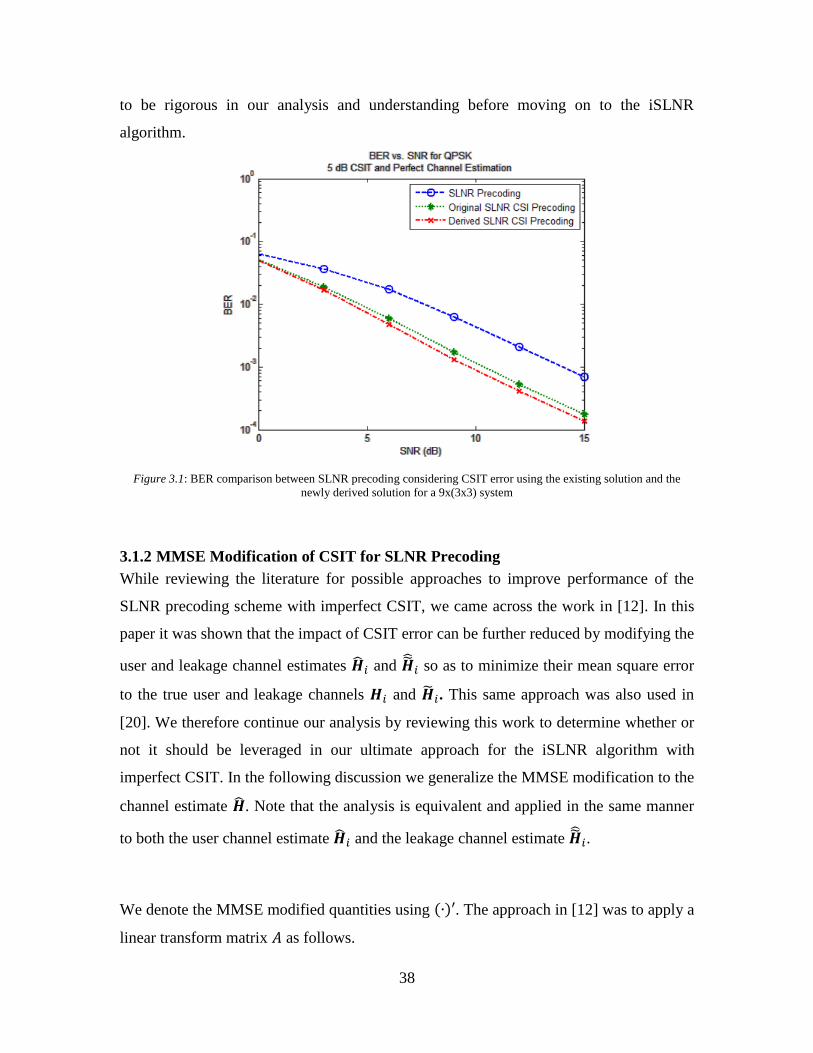
Figure 3.1 shows a comparison between the bit error rates achieved by a 9x(3x3) system

using the SLNR precoding scheme without considering imperfect CSIT, the previously

proposed SLNR precoding scheme considering imperfect CSIT, and our newly derived

SLNR precoding scheme considering imperfect CSIT. In this simulation the CSIT is 5

dB. The first observation from these results is that both of the schemes considering the

CSIT error statistics perform significantly better than the scheme which does not. At an

error rate of 1e-3 there is approximately 6 dB of gain. We also observe that the newly

derived approach provides better error rate performance than the previously proposed

solution as it more accurately accounts for the distribution of 𝑯𝑖 given �̂�𝑖. The difference

in performance is somewhat marginal; about 0.6 dB at an error rate of 1e-3, but we want

38

to be rigorous in our analysis and understanding before moving on to the iSLNR

algorithm.

Figure 3.1: BER comparison between SLNR precoding considering CSIT error using the existing solution and the

newly derived solution for a 9x(3x3) system

3.1.2 MMSE Modification of CSIT for SLNR Precoding

While reviewing the literature for possible approaches to improve performance of the

SLNR precoding scheme with imperfect CSIT, we came across the work in [12]. In this

paper it was shown that the impact of CSIT error can be further reduced by modifying the

user and leakage channel estimates �̂�𝑖 and �̂̃�𝑖 so as to minimize their mean square error

to the true user and leakage channels 𝑯𝑖 and �̃�𝑖. This same approach was also used in

[20]. We therefore continue our analysis by reviewing this work to determine whether or

not it should be leveraged in our ultimate approach for the iSLNR algorithm with

imperfect CSIT. In the following discussion we generalize the MMSE modification to the

channel estimate �̂�. Note that the analysis is equivalent and applied in the same manner

to both the user channel estimate �̂�𝑖 and the leakage channel estimate �̂̃�𝑖.

We denote the MMSE modified quantities using (∙)′. The approach in [12] was to apply a

linear transform matrix 𝐴 as follows.

39

𝑯′ ≜ �̂�𝑨 (55)

The mean square error of the channel estimate from the true channel is given by

𝑀𝑆𝐸 = 𝐸{‖𝑯′ − 𝑯‖2} (56)

It was then shown that the matrix 𝑨 which will minimize the mean square error is

𝑨 = (𝑀𝜎𝑐2𝑰 + 𝑯∗𝑯)𝑯∗𝑯

(57)

It was further shown that using this approach reduces the CSIT error variance and the

modified CSIT error variance is then given by

𝜎𝑐

2′ =𝜎𝑐

2

𝑟∑

𝜆𝑖

𝜆𝑖 + 𝜎𝑐2

𝑟

𝑖=1

(58)

where 𝑟 is the rank and 𝜆𝑖 is the 𝑖𝑡ℎ eigenvalue of the transmit covariance matrix. The

modified CSIT and modified error variances are then substituted directly into the original

solution for the SLNR precoding matrix under imperfect CSIT (given in equation 45) as

follows


(

(�̃�𝑖′∗�̃�𝑖

′ + ( ∑ 𝑀𝑗

𝐾

𝑗=1,𝑗≠𝑖

𝜎𝑐2′ +

𝑀𝑖


2) 𝑰)

−1

(𝑯𝑖′∗𝑯𝑖

′ + 𝜎𝑐2′𝑰)

)

(59)

The issue we note with this approach is that the expression for 𝑨 given in equation 57

depends on the actual channel 𝑯 rather than the estimated channel �̂�. This presents an

issue because the transmitter will only have knowledge of �̂� in practice. Indeed if the

transmitter has knowledge of 𝑯, then it already possesses an error free channel estimate

and the entire problem is effectively avoided by using 𝑯 directly. So in practice the

approach used in [12,20] is only useful if �̂� can be substituted for 𝑯 as in

𝑨 = (𝑀𝜎𝑐2𝑰 + �̂�∗�̂�)�̂�∗�̂�

(60)

40

As we’ll show later, the more practical solution in equation 60 will still manage to reduce

the CSIT MSE, but it will not minimize it. In addition, we note that the authors of [12]

reused the solution proposed in [7] for SLNR precoding with imperfect CSIT whereas we

have shown that the newly derived solution results in better performance.

While there are certain issues with the particular approach used to minimize the mean

square error shown in [12], it still seems reasonable that the SLNR precoding might

benefit from modifying the CSIT to meet the MMSE criteria. So rather than using the

solution proposed in [12] directly, we instead move to derive the MMSE modification

which will rely only on knowledge of �̂� and the second-order statistics of the CSIT error,

𝜎𝑐2. We begin in a similar fashion with the expression for the MSE between the modified

channel estimate 𝑯′ and the actual channel 𝑯, conditioned on the unmodified channel

estimate �̂�.

𝑀𝑆𝐸 = 𝐸{‖𝑯′ − 𝑯‖2 | �̂�}

= 𝐸 {‖�̂�𝑨 − 𝑯‖2 | �̂�}

= 𝐸{𝑇𝑟[(�̂�𝑨 − 𝑯)∗(�̂�𝑨 − 𝑯)] | �̂�}

= 𝐸{𝑇𝑟[𝑨∗�̂�∗�̂�𝑨 − 𝑨∗�̂�∗𝑯 − 𝑯∗�̂�𝑨 + 𝑯∗𝑯] | �̂�} (61)

The trace of a matrix is a linear operator and so may be exchanged with the expectation.

= 𝑇𝑟[𝑨∗�̂�∗�̂�𝑨 − 𝑨∗𝑬{�̂�∗𝑯| �̂�} − 𝐸{𝑯∗�̂�| �̂�}𝑨 + 𝐸{𝑯∗𝑯| �̂�}] (62)

As in section 3.1.1 we utilize the distribution of 𝑯 conditioned on �̂� given below

𝑝(𝑯|�̂�) = 𝜌ℎ�̂� + 𝛀 (63)

Substituting this expression into equation 62 we have

= 𝑇𝑟[𝑨∗�̂�∗�̂�𝑨 − 𝑨∗𝑬{�̂�∗(𝜌ℎ�̂� + 𝛀)| �̂�} − 𝐸{(𝜌ℎ�̂� + 𝛀)∗�̂�| �̂�}𝑨

+ 𝐸{(𝜌ℎ�̂� + 𝛀)∗(𝜌ℎ�̂� + 𝛀)| �̂�}]

41

which simplifies to

= 𝑇𝑟[𝑨∗�̂�∗�̂�𝑨 − 𝜌ℎ𝑨∗�̂�∗�̂� − 𝜌ℎ�̂�∗�̂�𝑨 + 𝜌ℎ𝟐�̂�∗�̂� + 𝑀𝜌ℎ𝑰 ]

(64)

In order to minimize this MSE, we take the gradient with respect to 𝑨 and set it equal to

zero.

∇𝑨(𝑀𝑆𝐸) = 2𝑨∗�̂�∗�̂� − 𝜌ℎ�̂�∗�̂� − 𝜌ℎ�̂�∗�̂� = 𝟎

= 2𝑨∗�̂�∗�̂� − 2𝜌ℎ�̂�∗�̂� = 𝟎 (65)

from which we arrive at

𝑨 = 𝜌ℎ�̂�∗�̂�(�̂�∗�̂�)−1

𝑨 = 𝜌ℎ𝑰 (66)

So the candidate 𝑨, to minimize the mean square error of the CSIT error is given in

equation 66. We then derive the Hessian of the MSE with respect to 𝑨

∇𝑨𝟐(𝑀𝑆𝐸) = 2�̂�∗�̂�

(67)

which is trivially noted to be a positive semi-definite matrix, making 𝑨 the global

minimizer of the MSE.

From equation 66 we see that only a scalar modification is needed to minimize the mean

square error of the channel estimate. We therefore redefine the modified CSIT using a

scalar modification as

𝑯′ ≜ 𝛼�̂� (68)

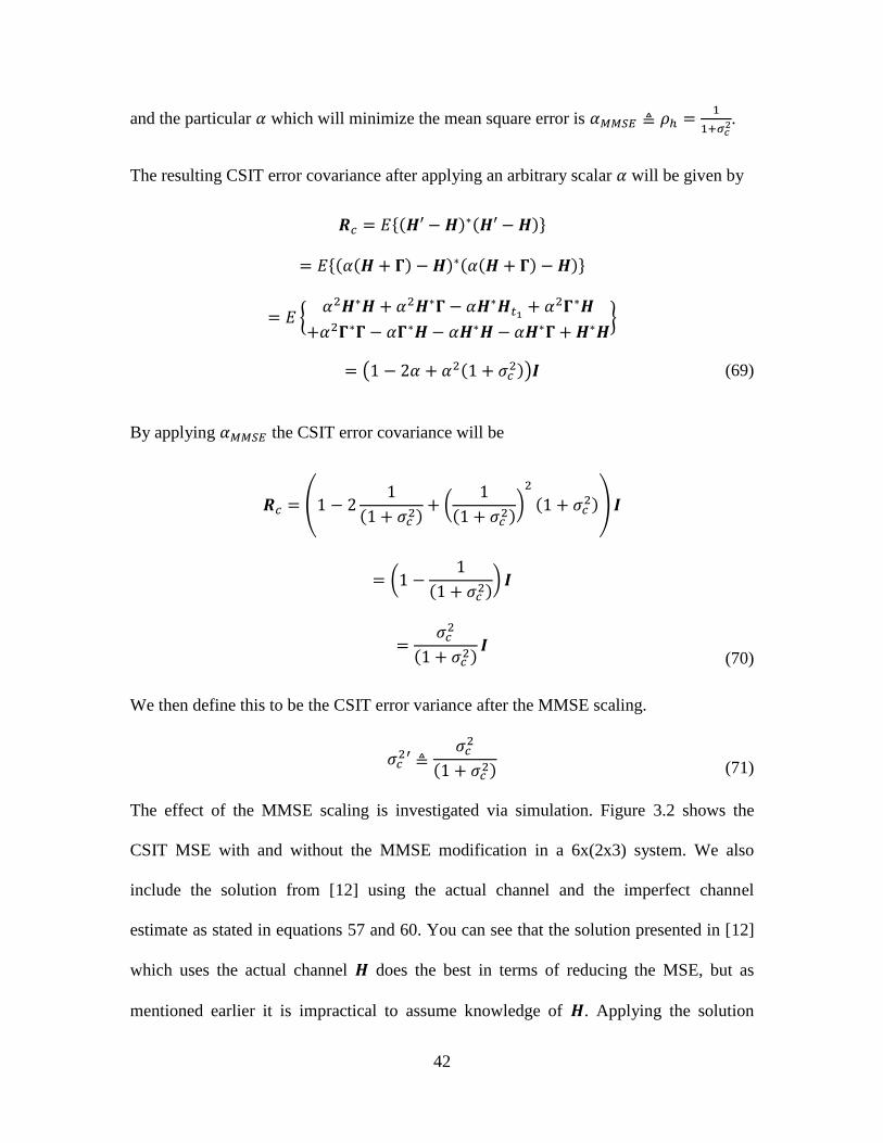
42

and the particular 𝛼 which will minimize the mean square error is 𝛼𝑀𝑀𝑆𝐸 ≜ 𝜌ℎ =1

1+𝜎𝑐2.

The resulting CSIT error covariance after applying an arbitrary scalar 𝛼 will be given by

𝑹𝑐 = 𝐸{(𝑯′ − 𝑯)∗(𝑯′ − 𝑯)}

= 𝐸{(𝛼(𝑯 + 𝚪) − 𝑯)∗(𝛼(𝑯 + 𝚪) − 𝑯)}

= 𝐸 {𝛼2𝑯∗𝑯 + 𝛼2𝑯∗𝚪 − 𝛼𝑯∗𝑯𝑡1 + 𝛼2𝚪∗𝑯

+𝛼2𝚪∗𝚪 − 𝛼𝚪∗𝑯 − 𝛼𝑯∗𝑯 − 𝛼𝑯∗𝚪 + 𝑯∗𝑯}

= (1 − 2𝛼 + 𝛼2(1 + 𝜎𝑐2))𝑰 (69)

By applying 𝛼𝑀𝑀𝑆𝐸 the CSIT error covariance will be

𝑹𝑐 = (1 − 21

(1 + 𝜎𝑐2)

+ (1

(1 + 𝜎𝑐2)

)2

(1 + 𝜎𝑐2)) 𝑰

= (1 −1

(1 + 𝜎𝑐2)

) 𝑰

=

𝜎𝑐2

(1 + 𝜎𝑐2)

𝑰 (70)

We then define this to be the CSIT error variance after the MMSE scaling.

𝜎𝑐

2′ ≜𝜎𝑐

2

(1 + 𝜎𝑐2)

(71)

The effect of the MMSE scaling is investigated via simulation. Figure 3.2 shows the

CSIT MSE with and without the MMSE modification in a 6x(2x3) system. We also

include the solution from [12] using the actual channel and the imperfect channel

estimate as stated in equations 57 and 60. You can see that the solution presented in [12]

which uses the actual channel 𝑯 does the best in terms of reducing the MSE, but as

mentioned earlier it is impractical to assume knowledge of 𝑯. Applying the solution

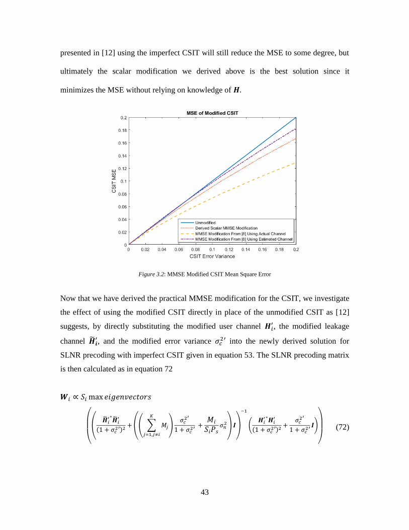
43

presented in [12] using the imperfect CSIT will still reduce the MSE to some degree, but

ultimately the scalar modification we derived above is the best solution since it

minimizes the MSE without relying on knowledge of 𝑯.

Figure 3.2: MMSE Modified CSIT Mean Square Error

Now that we have derived the practical MMSE modification for the CSIT, we investigate

the effect of using the modified CSIT directly in place of the unmodified CSIT as [12]

suggests, by directly substituting the modified user channel 𝑯𝑖′, the modified leakage

channel �̃�𝒊′, and the modified error variance 𝜎𝑐

2′ into the newly derived solution for

SLNR precoding with imperfect CSIT given in equation 53. The SLNR precoding matrix

is then calculated as in equation 72

𝑾𝑖 ∝ 𝑆𝑖 max 𝑒𝑖𝑔𝑒𝑛𝑣𝑒𝑐𝑡𝑜𝑟𝑠

(

(�̃�𝑖

′∗�̃�𝑖′

(1 + 𝜎𝑐2′)2

+ (( ∑ 𝑀𝑗

𝐾

𝑗=1,𝑗≠𝑖

)𝜎𝑐

2′

1 + 𝜎𝑐2′

+𝑀𝑖


2)𝑰)

−1

(𝑯𝑖

′∗𝑯𝑖′

(1 + 𝜎𝑐2′)2

+𝜎𝑐

2′

1 + 𝜎𝑐2′

𝑰)

)

(72)

44

Figure 3.3 shows the bit error rate of a 9x(3x3) system operating with 5 dB CSIT using

the derived SLNR precoding scheme which considers CSIT error, both with the

unmodified CSIT and with the MMSE modified CSIT. The previously derived SLNR

precoding scheme with imperfect CSIT is also included. From these results we observe

that the practical MMSE modification provides a marginal gain, less than was shown by

the results in [12]. In this case, at an error rate of 1e-3 it provides about 0.4 dB of gain

compared to the newly derived SLNR precoding with imperfect CSIT and about 1 dB

compared to the original SLNR precoding with imperfect CSIT from [7].

Figure 3.3: Bit error rate with MMSE modification of CSIT

3.2 iSLNR Precoding Considering CSIT Error

Now that we have considered how we may best mitigate the effects of imperfect CSIT

using the non-iterative SLNR precoding scheme, we will continue on to apply similar

analysis to the iterative algorithm. As explained in chapter two, the iSLNR algorithm

relies on calculating the receiver processing for each user to then update effective leakage

channels and recalculate the precoding matrices. We must then consider the effects of

imperfect CSIT both in the calculation of receiver processing and precoding matrices in

order to achieve the best possible performance using this algorithm with imperfect CSIT.

45

3.2.1 Receiver Calculation with Imperfect CSIT

With perfect CSIT and CSIR, the receive filters are calculated without error using

equation 15 for ZF receivers and equations 17 and 20 for IRC receivers. With imperfect

CSIT this is no longer true, which motivates us to investigate the calculation of receive

filters in the iSLNR algorithm with imperfect CSIT. Note that in the following

derivations we have dropped the user index to ease notation, though the reader should

note that all quantities are specific to a particular user.

We begin by considering the interference plus noise covariance matrix given in equation

18 which is required to calculate the IRC receiver structure. With perfect CSIT this

expression would be conditioned on the true channel 𝑯 and the interference precoding

matrix 𝑾𝑛, which is ultimately how we arrived at the expression in equation 20. In this

case the expression is conditioned on the channel estimate �̂� and the interference

precoding matrix 𝑾𝑛 as shown below.

�̂�𝑛 = 𝐸{( 𝑯𝑾𝑛𝒔𝑛 + 𝒏)(𝑯𝑾𝑛𝒔𝑛 + 𝒏)∗ | �̂�,𝑾𝑛} (73)

We substitute the distribution of 𝑯 given �̂� into the equation

= 𝐸 {( (𝜌ℎ�̂� + 𝛀)𝑾𝑛𝒔𝑛 + 𝒏) ((𝜌ℎ�̂� + 𝛀)𝑾𝑛𝒔𝑛 + 𝒏)∗

| �̂�,𝑾𝑛} (74)

Where again 𝜌ℎ =1

1+𝜎𝑐2 and the elements of 𝛀 are i.i.d. complex Gaussian random

variables with zero mean and variance 𝜎𝑐

2

1+𝜎𝑐2. We expand this expression as follows.

= 𝐸 {( (𝜌ℎ�̂� + 𝛀)𝑾𝑛𝒔𝑛) ((𝜌ℎ�̂� + 𝛀)𝑾𝑛𝒔𝑛)∗

+ ( (𝜌ℎ�̂� + 𝛀)𝑾𝑛𝒔𝑛)𝒏∗

+ 𝒏( (𝜌ℎ�̂� + 𝛀)𝑾𝑛𝒔𝑛)∗+ 𝒏𝒏∗| �̂�,𝑾𝑛}

(75)

By noting that the noise term is independent of all other terms and has zero mean we can

simplify.

46

= 𝐸 {( (𝜌ℎ�̂� + 𝛀)𝑾𝑛𝒔𝑛) ((𝜌ℎ�̂� + 𝛀)𝑾𝑛𝒔𝑛)∗

| �̂�,𝑾𝑛} + 𝐸{𝒏𝒏∗} (76)

We then continue by expanding the expression on the left.

= 𝐸{𝜌ℎ2�̂�𝑾𝑛𝒔𝑛𝒔𝑛

∗ 𝑾𝑛∗ �̂�∗ + 𝜌ℎ�̂�𝑾𝑛𝒔𝑛𝒔𝑛

∗ 𝑾𝑛∗ 𝛀∗ + 𝜌ℎ𝛀𝑾𝑛𝒔𝑛𝒔𝑛

∗ 𝑾𝑛∗ �̂�∗

+ 𝛀𝑾𝑛𝒔𝑛𝒔𝑛∗ 𝑾𝑛

∗ 𝛀∗| �̂�,𝑾𝑛} + 𝐸{𝒏𝒏∗} (77)

We can again simplify by noting that �̂� and 𝛀 are independent and by treating 𝒔𝑛 as a

random variable with unit power and uniformly distributed phase. This results in the

following expression.

= 𝐸{𝜌ℎ2�̂�𝑾𝑛𝑾𝑛

∗ �̂�∗ + 𝛀𝑾𝑛𝑾𝑛∗ 𝛀∗| �̂�,𝑾𝑛} + 𝐸{𝒏𝒏∗} (78)

Since �̂� and 𝑾𝑛 are given quantities, the expectation can be removed.

= 𝜌ℎ2�̂�𝑾𝑛𝑾𝑛

∗ �̂�∗ + 𝐸{𝛀𝑾𝑛𝑾𝑛∗ 𝛀∗} + 𝐸{𝒏𝒏∗} (79)

The 𝐸{𝒏𝒏∗} term is very easily seen to be 𝜎𝑛2𝑰, though it’s maybe not quite as obvious

how the 𝐸{𝛀𝑾𝑛𝑾𝑛∗ 𝛀∗} term simplifies. We therefore show it explicitly here using an

example scenario to avoid the more complex notation needed to make the expressions

general. We consider a 6x(2x4) system with a single stream per user. In this case, for user

1 we have

𝛀𝑾𝑛 = [𝜔11 𝜔12

𝜔21 𝜔22

𝜔13 𝜔14

𝜔23 𝜔24

𝜔15 𝜔16

𝜔25 𝜔26]

[ 𝑤21

𝑤22

𝑤23

𝑤31

𝑤32

𝑤33

𝑤41

𝑤42

𝑤43𝑤24

𝑤25

𝑤26

𝑤34

𝑤35

𝑤36

𝑤44

𝑤45

𝑤46]

47

=

[ ∑ 𝜔1𝑘𝑤2𝑘

6

𝑘=1∑ 𝜔1𝑘𝑤3𝑘

6


6

𝑘=1

∑ 𝜔2𝑘𝑤2𝑘

6


6


6

𝑘=1 ]

= ∑ [

𝜔1𝑘𝑤2𝑘 𝜔1𝑘𝑤3𝑘 𝜔1𝑘𝑤4𝑘

𝜔2𝑘𝑤2𝑘 𝜔2𝑘𝑤3𝑘 𝜔2𝑘𝑤4𝑘]

6

𝑘=1

(80)

Using this expression we can rewrite 𝐸{𝛀𝑾𝑛𝑾𝑛∗ 𝛀∗} as

𝐸{𝛀𝑾𝑛𝑾𝑛∗ 𝛀∗}

= 𝐸 {∑ [𝜔1𝑗𝑤2𝑗 𝜔1𝑗𝑤3𝑗 𝜔1𝑗𝑤4𝑗

𝜔2𝑗𝑤2𝑗 𝜔2𝑗𝑤3𝑗 𝜔2𝑗𝑤4𝑗]∑ [

𝜔1𝑘∗ 𝑤2𝑘

∗ 𝜔2𝑘∗ 𝑤2𝑘

∗



∗



∗]

6

𝑘=1

6

𝑗=1}

(81)

We define the matrix 𝐶 = 𝐸{𝛀𝑾𝑛𝑾𝑛∗ 𝛀∗} = [

𝑏11 𝑏12

𝑏21 𝑏22] so we can reasonably write out

each element as below.

𝑐11 = 𝐸 {∑ (∑ 𝜔1𝑘𝑤𝑖𝑘

6

𝑘=1∑ 𝜔1𝑘

∗ 𝑤𝑖𝑘∗

6

𝑘=1)

4

𝑖=2}

𝑐12 = 𝐸 {∑ (∑ 𝜔1𝑘𝑤𝑖𝑘

6

𝑘=1∑ 𝜔2𝑘

∗ 𝑤𝑖𝑘∗

6

𝑘=1)

4

𝑖=2}

𝑐21 = 𝐸 {∑ (∑ 𝜔2𝑘𝑤𝑖𝑘

6

𝑘=1∑ 𝜔1𝑘

∗ 𝑤𝑖𝑘∗

6

𝑘=1)

4

𝑖=2}

𝑐22 = 𝐸 {∑ (∑ 𝜔2𝑘𝑤𝑖𝑘

6

𝑘=1∑ 𝜔2𝑘

∗ 𝑤𝑖𝑘∗

6

𝑘=1)

4

𝑖=2} (82)

Independence between 𝜔𝑖𝑗 and 𝑤𝑚𝑛 implies

𝐸{𝜔𝑖𝑗𝜔𝑖𝑗∗ 𝑤𝑚𝑛𝑤𝑚𝑛

∗ } = 𝐸{𝜔𝑖𝑗𝜔𝑖𝑗∗ }𝐸{𝑤𝑚𝑛𝑤𝑚𝑛

∗ } ∀ 𝑖, 𝑗, 𝑚, and 𝑛 (83)

With the elements of 𝛀 being i.i.d. we also have

𝐸{𝜔𝑖𝑗𝜔𝑚𝑛∗ } = 0 ∀ 𝑖 ≠ 𝑚 or 𝑗 ≠ 𝑛 (84)

Using the conditions in equations 83 and 84 we can simplify 𝑪 to the following

48

𝑪 =

[ ∑ ∑ 𝐸{𝜔1𝑘𝜔1𝑘

∗ }𝑤𝑖𝑘𝑤𝑖𝑘∗

6

𝑘=1

4

𝑖=20

0 ∑ ∑ 𝐸{𝜔2𝑘𝜔2𝑘∗ }𝑤𝑖𝑘𝑤𝑖𝑘

∗6

𝑘=1

4

𝑖=2 ]

(85)

Noting that 𝐸{𝜔𝑖𝑗𝜔𝑖𝑗∗ } =

𝜎𝑐2

1+𝜎𝑐2 ∀ 𝑖, 𝑗 this simplifies to

𝑪 =

[

𝜎𝑐2

1 + 𝜎𝑐2∑ ∑ 𝑤𝑖𝑘𝑤𝑖𝑘

∗6

𝑘=1

4

𝑖=20

0𝜎𝑐

2


∗6

𝑘=1

4

𝑖=2 ]

= (

𝜎𝑐2


∗6

𝑘=1

4

𝑖=2) 𝑰 (86)

In this work we have assumed equal power per stream given by 𝑃𝑠. This implies that

∑ 𝑤𝑖𝑘𝑤𝑖𝑘

∗6

𝑘=1= 𝑃𝑠 ∀ 𝑖 (87)

So the matrix 𝑪 simplifies further to

𝑪 = (𝜎𝑐

2

1 + 𝜎𝑐2∑ 𝑃𝑠

4

𝑖=2) 𝑰

= (3𝑃𝑠

𝜎𝑐2

1 + 𝜎𝑐2) 𝑰 (88)

We note that the factor of 3 comes from the total number of interfering streams so the

generalized expression in a system with 𝐾 users and where the 𝑗𝑡ℎ user has 𝑆𝑗 streams is

given by

49

𝑪 = 𝐸{𝛀𝑾𝑛𝑾𝑛

∗ 𝛀∗} = (𝑃𝑠 ∑ 𝑆𝑗

𝐾

𝑗=1,𝑗≠𝑖)

𝜎𝑐2

1 + 𝜎𝑐2𝑰 (89)

With this result in mind, we return to simplifying the expression for the interference plus

noise covariance matrix where we left off at equation 79. The final expression is given by

�̂�𝑛 =�̂�𝑾𝑛𝑾𝑛

∗ �̂�∗

(1 + 𝜎𝑐2)2

+ ((𝑃𝑠 ∑𝑆𝑘

𝐾

𝑘≠𝑖

)𝜎𝑐

2

1 + 𝜎𝑐2+ 𝜎𝑛

2) 𝑰 (90)

With a single stream per user and total transmit power 𝑃 = 1, this of course simplifies to

�̂�𝑛 =

�̂�𝑾𝑛𝑾𝑛∗ �̂�∗

(1 + 𝜎𝑐2)2

+ ((𝐾 − 1)

𝐾

𝜎𝑐2

1 + 𝜎𝑐2+ 𝜎𝑛

2) 𝑰 (91)

Now that we have found the expression for the interference plus noise covariance, we

look at the expression for the IRC receiver processing matrix provided in equation 17.

We note that this equation depends on the true channel 𝑯 whereas the transmitter only

has access to the estimated channel �̂�. We therefore desire to minimize the impact of the

estimation error on our calculation of �̂�𝐼𝑅𝐶. To do this we solve for the �̂�𝐼𝑅𝐶 which will

minimize the mean square error given by

𝑀𝑆𝐸 = 𝐸 {‖�̂�𝐼𝑅𝐶 − 𝑻𝐼𝑅𝐶‖2}

= 𝐸{(�̂�𝐼𝑅𝐶 − 𝑻𝐼𝑅𝐶)∗(�̂�𝐼𝑅𝐶 − 𝑻𝐼𝑅𝐶)}

= �̂�𝐼𝑅𝐶∗ �̂�𝐼𝑅𝐶 − �̂�𝐼𝑅𝐶

∗ 𝐸{𝑻𝐼𝑅𝐶} − 𝐸{𝑻𝐼𝑅𝐶∗ }�̂�𝐼𝑅𝐶 + 𝐸{𝑻𝐼𝑅𝐶

∗ 𝑻𝐼𝑅𝐶} (92)

Taking the gradient with respect to �̂�𝐼𝑅𝐶 and setting it to zero we have

∇𝑻𝐼𝑅𝐶(𝑀𝑆𝐸) = 2�̂�𝐼𝑅𝐶 − 2𝐸{𝑻𝐼𝑅𝐶} = 0

50

�̂�𝐼𝑅𝐶 = 𝐸{𝑻𝐼𝑅𝐶} (93)

This is a standard result as described in [23]. We therefore move to simplify this

expression for �̂�𝐼𝑅𝐶 given the known quantities �̂�, 𝑾, and �̂�𝑛.

�̂�𝐼𝑅𝐶 = 𝐸{𝑻𝐼𝑅𝐶| �̂�,𝑾, �̂�𝑛}

= 𝐸 {(𝑾∗𝑯∗�̂�𝑛−1𝑯𝑾)

−1𝑾∗𝑯∗�̂�𝑛

−1| �̂�,𝑾, �̂�𝑛} (94)

We again substitute the distribution of 𝑯 given �̂�.

= 𝐸 {(𝑾∗ (𝜌ℎ�̂�∗+ 𝛀∗

) �̂�𝑛−1(𝜌ℎ�̂� + 𝛀)𝑾)

−1𝑾∗ (𝜌ℎ�̂�

∗+ 𝛀∗

) �̂�𝑛−1| �̂�,𝑾, �̂�𝑛} (95)

We expand the terms in the inverse and simplify by noting independence between �̂� and

𝛀.

= 𝐸 {(𝜌ℎ2𝑾∗�̂�∗�̂�𝑛

−1�̂�𝑾 + 𝑾∗𝛀∗�̂�𝑛−1𝛀𝑾)

−1| �̂�,𝑾, �̂�𝑛} 𝜌

ℎ𝑾∗�̂�∗�̂�𝑛

−1 (96)

For the 𝑖𝑡ℎ user we have ‖𝑾‖2 = 𝑆𝑖𝑃𝑠. Substituting this and the value of 𝜌ℎ into the

solution used to calculate the IRC receiver processing in the iSLNR algorithm with

imperfect CSIT yields

= (

𝑾∗�̂�∗�̂�𝑛−1�̂�𝑾

(1 + 𝜎𝑐2)𝟐

+ 𝑇𝑟[�̂�𝑛−1]𝑆𝑖𝑃𝑠

𝜎𝑐2

1 + 𝜎𝑐2𝑰)

−1𝑾∗�̂�∗�̂�𝑛

−1

1 + 𝜎𝑐2

(97)

Similarly the calculation of the receiver processing using ZF receivers will be given by its

expectation in order to minimize the mean square error. Expanding this expression as

before we have

�̂�𝑍𝐹 = 𝐸{𝑇𝑍𝐹}

= 𝐸{(𝑾∗𝑯∗𝑯𝑾)−1𝑾∗𝑯∗ | �̂�,𝑾}

= 𝐸 {(𝑾∗(𝜌ℎ�̂�∗ + 𝛀∗)(𝜌

ℎ�̂� + 𝛀)𝑾)

−1𝑾∗(𝜌

ℎ�̂�∗ + 𝛀∗) | �̂�,𝑾}

= 𝐸 {(𝜌ℎ2𝑾∗�̂�∗�̂�𝑾 + 𝑾∗𝛀∗𝛀𝑾)

−1| �̂�,𝑾, �̂�𝑛} 𝜌

ℎ𝑾∗�̂�∗

51

= (

𝑾∗�̂�∗�̂�𝑾

(1 + 𝜎𝑐2)𝟐

+ 𝑆𝑖𝑃𝑠

𝜎𝑐2

1 + 𝜎𝑐2𝑰)

−1𝑾∗�̂�∗

1 + 𝜎𝑐2 (98)

3.2.2 Modified SLNR Precoding with Imperfect CSIT

In the previous section we derived how the receiver processing matrices should be

calculated at the transmitter in the iSLNR algorithm with imperfect CSIT. The next step

of the algorithm is to use these matrices to update the effective leakage channels, so we

must consider the impact of imperfect CSIT on this step as well.

The expression to derive the initial precoding weights follows from the newly derived

SLNR precoding scheme with imperfect CSIT provided in equation 53 and restated

below to remind the reader


((�̂̃�𝑖

∗�̂̃�𝑖

(1 + 𝜎𝑐2)2

+ (∑𝑀𝑘

𝑘≠𝑖

𝜎𝑐2

1 + 𝜎𝑐2 +

𝑀𝑖


2) 𝑰)

−1

(�̂�𝑖

∗�̂�𝑖

(1 + 𝜎𝑐2)2

+𝜎𝑐

2

1 + 𝜎𝑐2𝑰))

(99)

Under the assumption of equal power per stream and unit total transmit power the result

is then normalized such that

‖𝒘𝑠‖

2 =1


∀ 𝑠 (100)

Where 𝒘𝑠 is the 𝑠𝑡ℎ column in 𝑾.

For each of the subsequent iterations in the iSLNR algorithm we update the precoding

matrix using the modified SLNR metric which uses effective leakage channels as given

in equation 39 and shown below.

52

𝑚𝑆𝐿𝑁𝑅 =


𝑆𝑖𝜎𝑛2 + ‖�̅�𝑖𝑾𝑖‖2

(101)

With imperfect CSIT, the expression is conditioned on the user channel estimate and

effective leakage channel estimate

=𝐸{𝑇𝑟[𝑾𝑖

∗𝑯𝑖∗𝑯𝑖𝑾𝑖] | �̂�𝑖}

𝑆𝑖𝜎𝑛2 + 𝐸{𝑇𝑟[𝑾𝑖

∗�̅�𝑖∗�̅�𝑖𝑾𝑖] | �̂̅�𝑖}

=

𝑇𝑟[𝐸{𝑾𝑖∗𝑯𝑖

∗𝑯𝑖𝑾𝑖 | �̂�𝑖}]

𝑆𝑖𝜎𝑛2 + 𝑇𝑟 [𝐸{𝑾𝑖

∗�̅�𝑖∗�̅�𝑖𝑾𝑖 | �̂̅�𝑖}]

(102)

We must now expand this expression and maximize it as we have in previous sections.

Note that we have already simplified the expression in the numerator in our previous

work, so we focus our attention on the leakage term in the denominator. Since 𝑾𝑖 is not a

random variable, but a chosen quantity it can be removed from the expectation.

𝐸{𝑾𝑖∗�̅�𝑖

∗�̅�𝑖𝑾𝑖 | �̂̅�𝑖} = 𝑾𝑖∗𝐸{�̅�𝑖

∗�̅�𝑖 | �̂̅�𝑖}𝑾𝑖 (103)

So we are left to determine the expression for 𝐸{�̅�𝑖∗�̅�𝑖 | �̂̅�𝑖}. To consider the imperfect

CSIT we explicitly write out the operation used to update the entire effective channel

using the normalized receiver processing matrices that are calculated at the transmitter as

follows

�̌� =

[ �̌�1 𝟎𝟎 𝟎

⋯ 𝟎⋯ 𝟎

𝟎 �̌�2

𝟎 𝟎

⋯ 𝟎⋯ 𝟎

⋮ ⋮𝟎 𝟎

⋱ ⋮⋯ �̌�𝐾

𝟎 𝟎 ⋯ 𝟎 ]

[

𝑯1

𝑯2

⋮𝑯𝐾

] (104)

As mentioned earlier, the rows containing all zeros are needed to ensure the dimension of

�̌� is equal to the dimension of 𝑯 since this scheme is only applicable for non-full-rank

transmissions. The effective leakage channel for the 𝑖𝑡ℎ user is then of course

�̅�𝑖 = [�̌�1𝑯1, 𝟎, … , �̌�𝑖−1𝑯𝑖−1, 𝟎, �̌�𝑖+1𝑯𝑖+1, 𝟎, … , �̌�𝐾𝑯𝐾, 𝟎]𝑇 (105)

53

Substituting this into the expectation we intend to evaluate, 𝐸{�̅�𝑖∗�̅�𝑖 | �̂̅�𝑖}, we may

rewrite it using a summation as follows

𝐸{�̅�𝑖∗�̅�𝑖 | �̂̅�𝑖} = 𝐸 {( ∑ 𝑯𝑘

∗ �̌�𝑘∗ �̌�𝑘𝑯𝑘

𝐾

𝑘=1,𝑘≠𝑖

) | �̂�𝑘, �̌�𝑘} (106)

With imperfect CSIT we substitute the distribution for 𝑯𝑘 given �̂�𝑘 as in previous

derivations

= 𝐸 {( ∑ (𝜌ℎ�̂�𝑘∗ + 𝛀𝑘

∗)�̌�𝑘∗ �̌�𝑘(𝜌ℎ�̂�𝑘 + 𝛀𝑘)

𝐾

𝑘=1,𝑘≠𝑖

) | �̂�𝑘, �̌�𝑘} (107)

Again noting independence between �̂�𝑘 and 𝛀𝑘 this can be expanded and simplified to

= 𝐸 {( ∑ 𝜌ℎ2�̂�𝑘

∗ �̌�𝑘∗ �̌�𝑘�̂�𝑘 + 𝛀k

∗ �̌�𝑘∗ �̌�𝑘𝛀𝑘

𝐾

𝑘=1,𝑘≠𝑖

) | �̂�𝑘, �̌�𝑘} (108)

Noting that 𝑇𝑟[�̌�𝑘∗ �̌�𝑘] = 𝑆𝑘 and that �̂�𝑘 and �̌�𝑘 are given, this can be equivalently

expressed

= ∑�̂�𝑘

∗ �̌�𝑘∗ �̌�𝑘�̂�𝑘

(1 + 𝜎𝑐2)2

+ 𝑆𝑘

𝜎𝑐2

1 + 𝜎𝑐2 𝑰

𝐾

𝑘=1,𝑘≠𝑖

(109)

Recognizing that the term on the left is just a scaled version of the original expression

using the estimated effective leakage channels we can rewrite this as

= (

�̂̅�𝑖∗�̂̅�𝑖

(1 + 𝜎𝑐2)2

+ ∑𝑆𝑘

𝑘≠𝑖

𝜎𝑐2

1 + 𝜎𝑐2𝑰)

(110)

For a single stream per user this is of course

= (

�̂̅�𝑖∗�̂̅�𝑖

(1 + 𝜎𝑐2)2

+ (𝐾 − 1)𝜎𝑐

2

1 + 𝜎𝑐2𝑰) (111)

Substituting this back into equation 103 we have

54

𝐸{𝑾𝑖

∗�̅�𝑖∗�̅�𝑖𝑾𝑖 | �̂̅�𝑖} = 𝑾𝑖

∗ (�̂̅�𝑖

∗�̂̅�𝑖

(1 + 𝜎𝑐2)2

+ ∑𝑆𝑘

𝑘≠𝑖

𝜎𝑐2

1 + 𝜎𝑐2𝑰)𝑾𝑖 (112)

Now that we have determined the expression involving the effective leakage channel

used by the mSLNR metric, we remind the reader that the expression in the numerator of

the mSLNR expression in equation 102 simplifies to

=

�̂�𝑖∗�̂�𝑖

(1 + 𝜎𝑐2)2

+ 𝑀𝑖

𝜎𝑐2

1 + 𝜎𝑐2𝑰 (113)

With these two results we arrive at the expression for the modified SLNR metric as

shown below.

=

𝑇𝑟 [𝑾𝑖∗ (

�̂�𝑖∗�̂�𝑖

(1 + 𝜎𝑐2)2 + 𝑀𝑖

𝜎𝑐2

1 + 𝜎𝑐2 𝑰)𝑾𝑖]

𝑇𝑟 [𝑾𝑖∗ (

�̂̅�𝑖∗�̂̅�𝑖

(1 + 𝜎𝑐2)2 + (∑ 𝑆𝑘𝑘≠𝑖

𝜎𝑐2

1 + 𝜎𝑐2 +

1𝑃𝑠

𝜎𝑛2) 𝑰)𝑾𝑖]

(114)

Using the same eigenvalue decomposition approach as in previous derivations the

precoding weights which will maximize the modified SLNR considering imperfect CSIT

are given by


((�̂̅�𝑖

∗�̂̅�𝑖

(1 + 𝜎𝑐2)2

+ (∑ 𝑆𝑘

𝑘≠𝑖

𝜎𝑐2

1 + 𝜎𝑐2 +

1

𝑃𝑠𝜎𝑛

2) 𝑰)

−1

(�̂�𝑖

∗�̂�𝑖

(1 + 𝜎𝑐2)2

+ 𝑀𝑖

𝜎𝑐2

1 + 𝜎𝑐2 𝑰))

(115)

3.2.3 Simulation Results

In section 2.3 we saw that there was very little difference in the achieved sum-rate using

the iSLNR algorithm with ZF or IRC receivers with perfect CSIT. On the other hand,

Figure 3.4 highlights the significant gap in performance between the ZF and IRC receivers

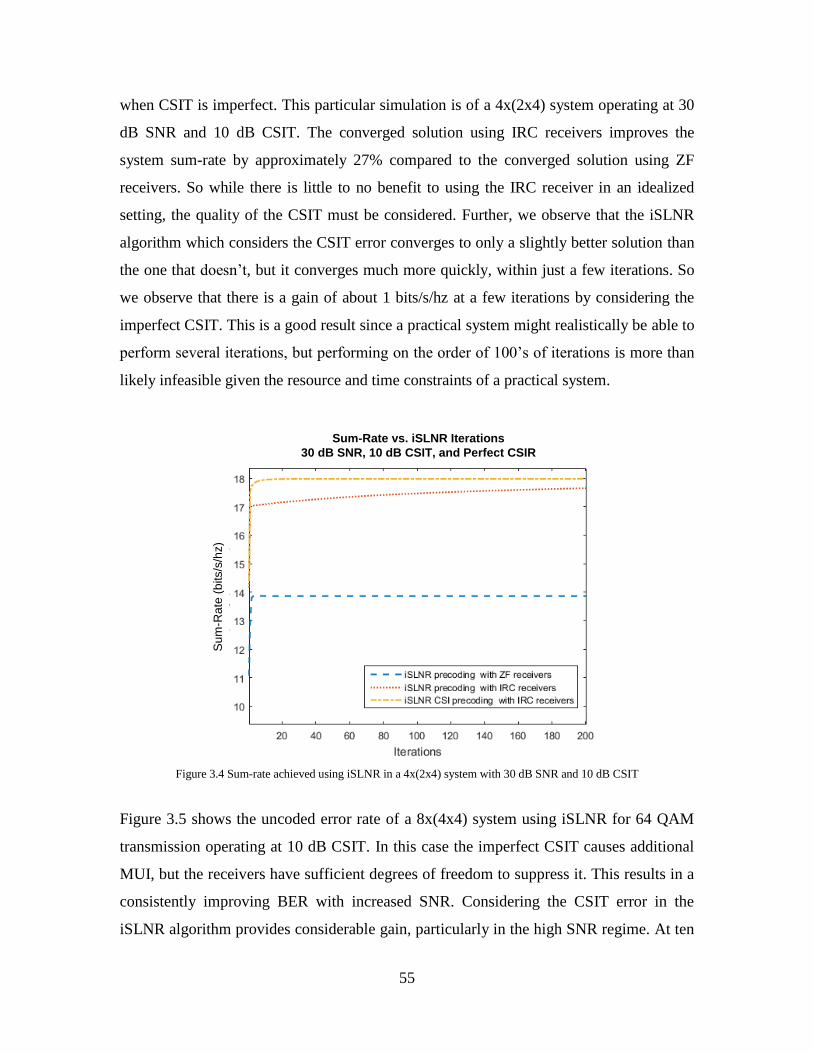
55

when CSIT is imperfect. This particular simulation is of a 4x(2x4) system operating at 30

dB SNR and 10 dB CSIT. The converged solution using IRC receivers improves the

system sum-rate by approximately 27% compared to the converged solution using ZF

receivers. So while there is little to no benefit to using the IRC receiver in an idealized

setting, the quality of the CSIT must be considered. Further, we observe that the iSLNR

algorithm which considers the CSIT error converges to only a slightly better solution than

the one that doesn’t, but it converges much more quickly, within just a few iterations. So

we observe that there is a gain of about 1 bits/s/hz at a few iterations by considering the

imperfect CSIT. This is a good result since a practical system might realistically be able to

perform several iterations, but performing on the order of 100’s of iterations is more than

likely infeasible given the resource and time constraints of a practical system.

Figure 3.4 Sum-rate achieved using iSLNR in a 4x(2x4) system with 30 dB SNR and 10 dB CSIT

Figure 3.5 shows the uncoded error rate of a 8x(4x4) system using iSLNR for 64 QAM

transmission operating at 10 dB CSIT. In this case the imperfect CSIT causes additional

MUI, but the receivers have sufficient degrees of freedom to suppress it. This results in a

consistently improving BER with increased SNR. Considering the CSIT error in the

iSLNR algorithm provides considerable gain, particularly in the high SNR regime. At ten

Sum-Rate vs. iSLNR Iterations

30 dB SNR, 10 dB CSIT, and Perfect CSIR

Su

m-R

ate

(b

its/s

/hz)

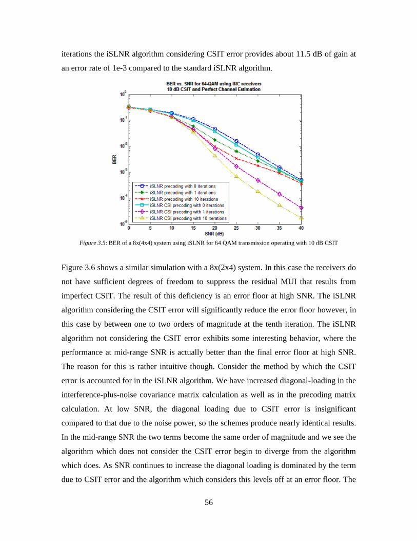
56

iterations the iSLNR algorithm considering CSIT error provides about 11.5 dB of gain at

an error rate of 1e-3 compared to the standard iSLNR algorithm.

Figure 3.5: BER of a 8x(4x4) system using iSLNR for 64 QAM transmission operating with 10 dB CSIT

Figure 3.6 shows a similar simulation with a 8x(2x4) system. In this case the receivers do

not have sufficient degrees of freedom to suppress the residual MUI that results from

imperfect CSIT. The result of this deficiency is an error floor at high SNR. The iSLNR

algorithm considering the CSIT error will significantly reduce the error floor however, in

this case by between one to two orders of magnitude at the tenth iteration. The iSLNR

algorithm not considering the CSIT error exhibits some interesting behavior, where the

performance at mid-range SNR is actually better than the final error floor at high SNR.

The reason for this is rather intuitive though. Consider the method by which the CSIT

error is accounted for in the iSLNR algorithm. We have increased diagonal-loading in the

interference-plus-noise covariance matrix calculation as well as in the precoding matrix

calculation. At low SNR, the diagonal loading due to CSIT error is insignificant

compared to that due to the noise power, so the schemes produce nearly identical results.

In the mid-range SNR the two terms become the same order of magnitude and we see the

algorithm which does not consider the CSIT error begin to diverge from the algorithm

which does. As SNR continues to increase the diagonal loading is dominated by the term

due to CSIT error and the algorithm which considers this levels off at an error floor. The

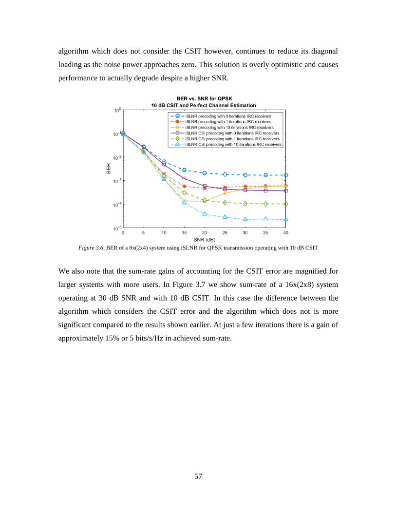
57

algorithm which does not consider the CSIT however, continues to reduce its diagonal

loading as the noise power approaches zero. This solution is overly optimistic and causes

performance to actually degrade despite a higher SNR.

Figure 3.6: BER of a 8x(2x4) system using iSLNR for QPSK transmission operating with 10 dB CSIT

We also note that the sum-rate gains of accounting for the CSIT error are magnified for

larger systems with more users. In Figure 3.7 we show sum-rate of a 16x(2x8) system

operating at 30 dB SNR and with 10 dB CSIT. In this case the difference between the

algorithm which considers the CSIT error and the algorithm which does not is more

significant compared to the results shown earlier. At just a few iterations there is a gain of

approximately 15% or 5 bits/s/Hz in achieved sum-rate.

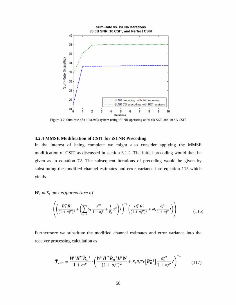
58

Figure 3.7: Sum-rate of a 16x(2x8) system using iSLNR operating at 30 dB SNR and 10 dB CSIT

3.2.4 MMSE Modification of CSIT for iSLNR Precoding

In the interest of being complete we might also consider applying the MMSE

modification of CSIT as discussed in section 3.1.2. The initial precoding would then be

given as in equation 72. The subsequent iterations of precoding would be given by

substituting the modified channel estimates and error variance into equation 115 which

yields


((�̅�𝑖

′∗�̅�𝑖′

(1 + 𝜎𝑐2′)2

+ (∑𝑆𝑘

𝑘≠𝑖

𝜎𝑐2′

1 + 𝜎𝑐2′

+1

𝑃𝑠

𝜎𝑛2) 𝑰)

−1

(𝑯𝑖

′∗𝑯𝑖′

(1 + 𝜎𝑐2′)2

+ 𝑀𝑖

𝜎𝑐2′

1 + 𝜎𝑐2′

𝑰)) (116)

Furthermore we substitute the modified channel estimates and error variance into the

receiver processing calculation as

�̂�𝐼𝑅𝐶 =

𝑾∗𝑯′∗�̂�𝑛−1

1 + 𝜎𝑐2′

∙ (𝑾∗𝑯′∗�̂�𝑛

−1𝑯′𝑾

(1 + 𝜎𝑐2′)𝟐

+ 𝑆𝑖𝑃𝑠𝑇𝑟[�̂�𝑛−1]

𝜎𝑐2′

1 + 𝜎𝑐2′

𝑰)

−1

(117)


30 dB SNR, 10 CSIT, and Perfect CSIR

Su

m-R

ate

(b

its/s

/hz)

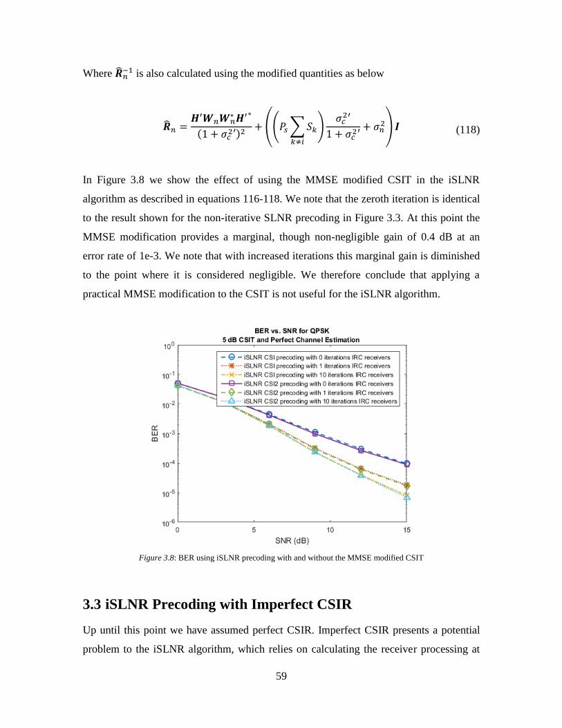
59

Where �̂�𝑛−1 is also calculated using the modified quantities as below

�̂�𝑛 =𝑯′𝑾𝑛𝑾𝑛

∗ 𝑯′∗

(1 + 𝜎𝑐2′)2

+ ((𝑃𝑠 ∑𝑆𝑘

𝑘≠𝑖

)𝜎𝑐

2′

1 + 𝜎𝑐2′

+ 𝜎𝑛2) 𝑰 (118)

In Figure 3.8 we show the effect of using the MMSE modified CSIT in the iSLNR

algorithm as described in equations 116-118. We note that the zeroth iteration is identical

to the result shown for the non-iterative SLNR precoding in Figure 3.3. At this point the

MMSE modification provides a marginal, though non-negligible gain of 0.4 dB at an

error rate of 1e-3. We note that with increased iterations this marginal gain is diminished

to the point where it is considered negligible. We therefore conclude that applying a

practical MMSE modification to the CSIT is not useful for the iSLNR algorithm.

Figure 3.8: BER using iSLNR precoding with and without the MMSE modified CSIT

3.3 iSLNR Precoding with Imperfect CSIR

Up until this point we have assumed perfect CSIR. Imperfect CSIR presents a potential

problem to the iSLNR algorithm, which relies on calculating the receiver processing at

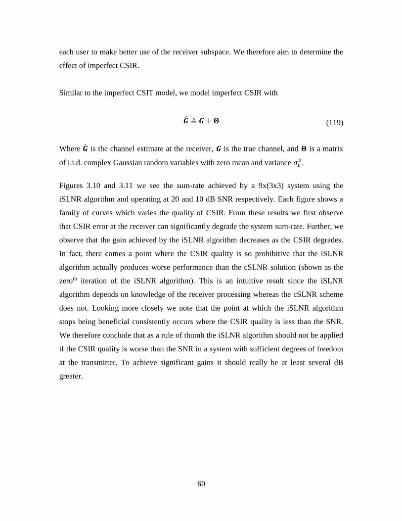
60

each user to make better use of the receiver subspace. We therefore aim to determine the

effect of imperfect CSIR.

Similar to the imperfect CSIT model, we model imperfect CSIR with

�́� ≜ 𝑮 + 𝚯 (119)

Where �́� is the channel estimate at the receiver, 𝑮 is the true channel, and 𝚯 is a matrix

of i.i.d. complex Gaussian random variables with zero mean and variance 𝜎𝑒2.

Figures 3.10 and 3.11 we see the sum-rate achieved by a 9x(3x3) system using the

iSLNR algorithm and operating at 20 and 10 dB SNR respectively. Each figure shows a

family of curves which varies the quality of CSIR. From these results we first observe

that CSIR error at the receiver can significantly degrade the system sum-rate. Further, we

observe that the gain achieved by the iSLNR algorithm decreases as the CSIR degrades.

In fact, there comes a point where the CSIR quality is so prohibitive that the iSLNR

algorithm actually produces worse performance than the cSLNR solution (shown as the

zeroth iteration of the iSLNR algorithm). This is an intuitive result since the iSLNR

algorithm depends on knowledge of the receiver processing whereas the cSLNR scheme

does not. Looking more closely we note that the point at which the iSLNR algorithm

stops being beneficial consistently occurs where the CSIR quality is less than the SNR.

We therefore conclude that as a rule of thumb the iSLNR algorithm should not be applied

if the CSIR quality is worse than the SNR in a system with sufficient degrees of freedom

at the transmitter. To achieve significant gains it should really be at least several dB

greater.

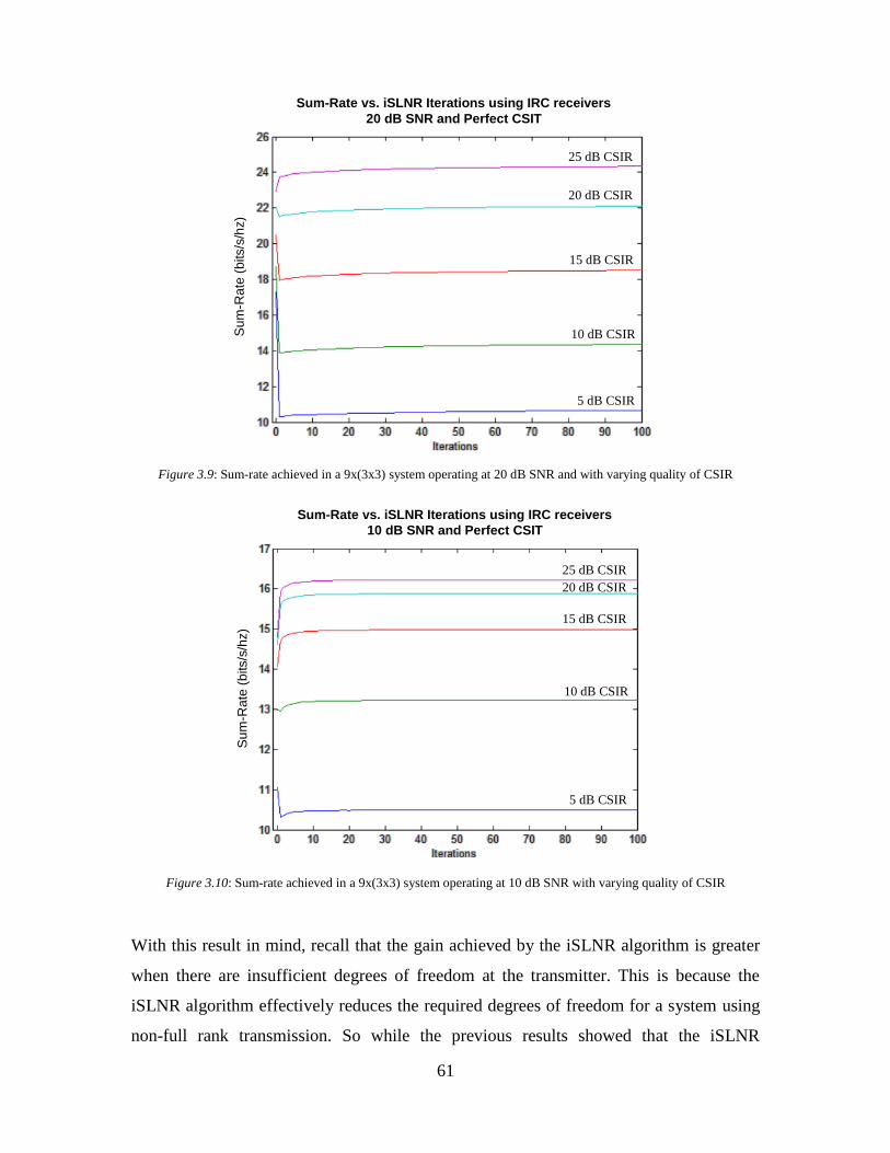
61

Figure 3.9: Sum-rate achieved in a 9x(3x3) system operating at 20 dB SNR and with varying quality of CSIR

Figure 3.10: Sum-rate achieved in a 9x(3x3) system operating at 10 dB SNR with varying quality of CSIR

With this result in mind, recall that the gain achieved by the iSLNR algorithm is greater

when there are insufficient degrees of freedom at the transmitter. This is because the

iSLNR algorithm effectively reduces the required degrees of freedom for a system using

non-full rank transmission. So while the previous results showed that the iSLNR

25 dB CSIR

20 dB CSIR

15 dB CSIR

10 dB CSIR

5 dB CSIR

5 dB CSIR

10 dB CSIR

15 dB CSIR

20 dB CSIR

25 dB CSIR


20 dB SNR and Perfect CSIT

Su

m-R

ate

(b

its/s

/hz)



Su

m-R

ate

(b

its/s

/hz)

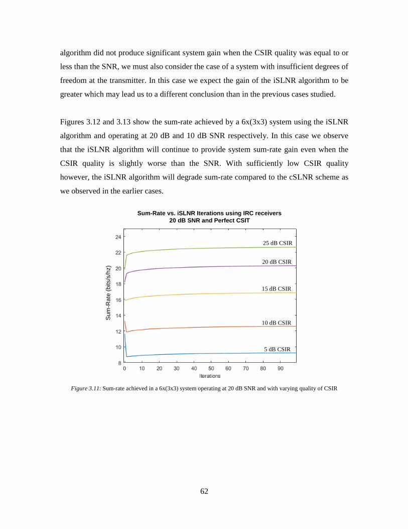
62

algorithm did not produce significant system gain when the CSIR quality was equal to or

less than the SNR, we must also consider the case of a system with insufficient degrees of

freedom at the transmitter. In this case we expect the gain of the iSLNR algorithm to be

greater which may lead us to a different conclusion than in the previous cases studied.

Figures 3.12 and 3.13 show the sum-rate achieved by a 6x(3x3) system using the iSLNR

algorithm and operating at 20 dB and 10 dB SNR respectively. In this case we observe

that the iSLNR algorithm will continue to provide system sum-rate gain even when the

CSIR quality is slightly worse than the SNR. With sufficiently low CSIR quality

however, the iSLNR algorithm will degrade sum-rate compared to the cSLNR scheme as

we observed in the earlier cases.


25 dB CSIR

20 dB CSIR

15 dB CSIR

10 dB CSIR

5 dB CSIR



Su

m-R

ate

(b

its/s

/hz)

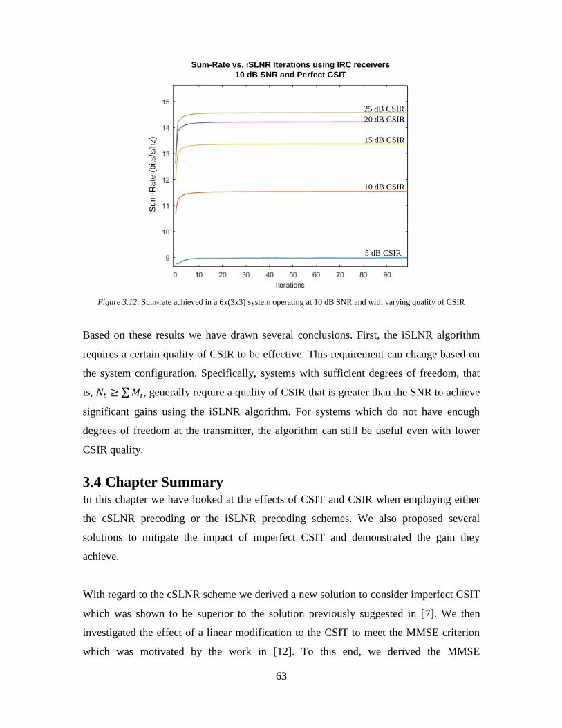
63


Based on these results we have drawn several conclusions. First, the iSLNR algorithm

requires a certain quality of CSIR to be effective. This requirement can change based on

the system configuration. Specifically, systems with sufficient degrees of freedom, that

is, 𝑁𝑡 ≥ ∑𝑀𝑖, generally require a quality of CSIR that is greater than the SNR to achieve

significant gains using the iSLNR algorithm. For systems which do not have enough

degrees of freedom at the transmitter, the algorithm can still be useful even with lower

CSIR quality.

3.4 Chapter Summary In this chapter we have looked at the effects of CSIT and CSIR when employing either

the cSLNR precoding or the iSLNR precoding schemes. We also proposed several

solutions to mitigate the impact of imperfect CSIT and demonstrated the gain they

achieve.

With regard to the cSLNR scheme we derived a new solution to consider imperfect CSIT

which was shown to be superior to the solution previously suggested in [7]. We then

investigated the effect of a linear modification to the CSIT to meet the MMSE criterion

which was motivated by the work in [12]. To this end, we derived the MMSE

25 dB CSIR

20 dB CSIR

15 dB CSIR

10 dB CSIR

5 dB CSIR



Su

m-R

ate

(b

its/s

/hz)

64

modification which avoids relying on the true channel value; an impractical requirement.

It was shown that applying this MMSE modification can provide a marginal though non-

negligible gain for the cSLNR scheme.

For the iSLNR algorithm we derived a method to calculate the receiver processing

matrices and the precoding matrices in a manner that accounts for the CSIT error. Using

these newly derived expressions showed improved performance in terms of system sum-

rate and error rate compared to the original iSLNR algorithm. We then applied the same

MMSE modification as used for the cSLNR scheme. Ultimately the gain achieved by

applying this modification was diminished after several iterations of the algorithm to the

point where it was considered negligible and removed from consideration.

We then went on to investigate the effects of CSIR error. From simulation we showed

first that with high CSIR error the iSLNR algorithm can actually reduce system

performance compared to the cSLNR solution. We demonstrated that when a system has

sufficient degrees of freedom to fully suppress the multiuser-interference, the iSLNR

algorithm will only provide system gain when the quality of the CSIR is greater than the

SNR. On the other hand in a system with insufficient degrees of freedom, the iSLNR

algorithm may provide non-trivial system gains even when the quality of the CSIR is less

than the SNR.

We also want to mention a fundamental tradeoff that exists between the iSLNR algorithm

and other joint transmit/receive processing design algorithms mentioned in the initial

introduction to the iSLNR algorithm in Chapter 2. This tradeoff is highlighted by the

work regarding CSIR error. A nice benefit of the iSLNR algorithm is that it considers the

receiver processing with no additional overhead; neither sending calculated processing

matrices to the users nor receiving user processing matrices to consider in the precoding

formulation. The drawback is that this makes the system performance more susceptible to

degradation due to CSIR error. If the receiver processing matrices were sent explicitly

then the precoding could be designed with full confidence in the receiver processing. Of

course, using explicitly signaled receiver processing matrices would also suffer from

65

being limited to a quantized codebook besides the additional overhead signaling. All of

these tradeoffs must be considered to achieve the best system design.

66

Chapter 4

Additional Considerations

In this chapter we investigate several other practical considerations for the iSLNR

algorithm. We begin by discussing the impact of transmit antenna correlation on the

achievable sum-rate. We then move on to consider the impact of time-varying channels

and how the iSLNR algorithm considering imperfect CSIT might be applied in this

setting. We then propose a method to improve the convergence of the iSLNR algorithm

with IRC receivers. Finally, we investigate tradeoffs in selecting the number of co-

scheduled users for the iSLNR algorithm.

4.1 The Effect of Transmit Antenna Correlation

In the previous analysis we have assumed the channel to be spatially white. This is a

reasonable assumption when the angles-of-arrival/departure for the multi-path scatterers

are uniformly distributed around both the transmit and receive antenna arrays, but if the

angles-of-arrival/departure follow a more narrow distribution then the channel will

exhibit spatial correlation. In a practical system it is common for the angles-of-

arrival/departure to follow a more narrow distribution at the base station than at the

mobile since the base station antennas will typically be placed high, away from

significant nearby scatterers. The angles-of-arrival/departure at the mobile will be closer

to a uniform distribution due to its low physical placement among many potential

scatterers. With this in mind, the effects of transmit antenna correlation at the base station

is of interest since this work focuses on the downlink.

A system with 𝑁 transmit antennas and 𝑀 receive antennas will have an 𝑁𝑀x𝑁𝑀

channel correlation matrix denoted 𝑹. In general each element of this matrix, 𝑟𝑖,𝑗, is

unique with the exception that 𝑟𝑖,𝑗 = 𝑟𝑗,𝑖∗ since correlation matrices must be Hermitian,

and the elements along the diagonal must be equal to one since each channel is perfectly

correlated with itself. For the purpose of simplified analysis, the Kronecker assumption is

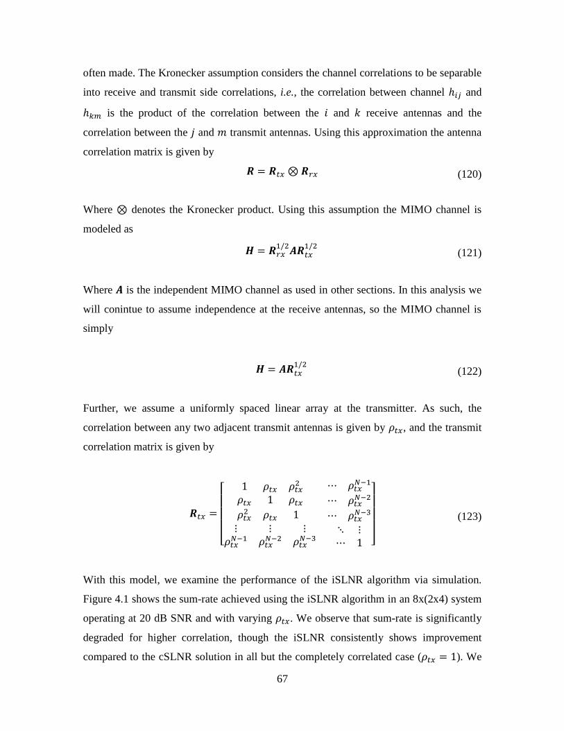
67

often made. The Kronecker assumption considers the channel correlations to be separable

into receive and transmit side correlations, i.e., the correlation between channel ℎ𝑖𝑗 and

ℎ𝑘𝑚 is the product of the correlation between the 𝑖 and 𝑘 receive antennas and the

correlation between the 𝑗 and 𝑚 transmit antennas. Using this approximation the antenna

correlation matrix is given by

𝑹 = 𝑹𝑡𝑥 ⊗ 𝑹𝑟𝑥 (120)

Where ⊗ denotes the Kronecker product. Using this assumption the MIMO channel is

modeled as

𝑯 = 𝑹𝑟𝑥1/2

𝑨𝑹𝑡𝑥1/2

(121)

Where 𝑨 is the independent MIMO channel as used in other sections. In this analysis we

will conintue to assume independence at the receive antennas, so the MIMO channel is

simply

𝑯 = 𝑨𝑹𝑡𝑥1/2

(122)

Further, we assume a uniformly spaced linear array at the transmitter. As such, the

correlation between any two adjacent transmit antennas is given by 𝜌𝑡𝑥, and the transmit

correlation matrix is given by

𝑹𝑡𝑥 =

[

1 𝜌𝑡𝑥 𝜌𝑡𝑥2

𝜌𝑡𝑥 1 𝜌𝑡𝑥

𝜌𝑡𝑥2 𝜌𝑡𝑥 1

⋯ 𝜌𝑡𝑥𝑁−1



⋮ ⋮ ⋮𝜌𝑡𝑥

𝑁−1 𝜌𝑡𝑥𝑁−2 𝜌𝑡𝑥

𝑁−3⋱ ⋮⋯ 1 ]

(123)

With this model, we examine the performance of the iSLNR algorithm via simulation.

Figure 4.1 shows the sum-rate achieved using the iSLNR algorithm in an 8x(2x4) system

operating at 20 dB SNR and with varying 𝜌𝑡𝑥. We observe that sum-rate is significantly

degraded for higher correlation, though the iSLNR consistently shows improvement

compared to the cSLNR solution in all but the completely correlated case (𝜌𝑡𝑥 = 1). We

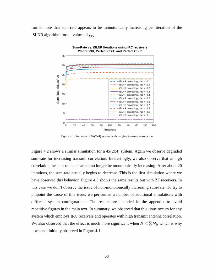
68

further note that sum-rate appears to be monotonically increasing per iteration of the

iSLNR algorithm for all values of 𝜌𝑡𝑥.

Figure 4.1: Sum-rate of 8x(2x4) system with varying transmit correlation

Figure 4.2 shows a similar simulation for a 4x(2x4) system. Again we observe degraded

sum-rate for increasing transmit correlation. Interestingly, we also observe that at high

correlation the sum-rate appears to no longer be monotonically increasing. After about 20

iterations, the sum-rate actually begins to decrease. This is the first simulation where we

have observed this behavior. Figure 4.3 shows the same results but with ZF receivers. In

this case we don’t observe the issue of non-monotonically increasing sum-rate. To try to

pinpoint the cause of this issue, we performed a number of additional simulations with

different system configurations. The results are included in the appendix to avoid

repetitive figures in the main text. In summary, we observed that this issue occurs for any

system which employs IRC receivers and operates with high transmit antenna correlation.

We also observed that the effect is much more significant when 𝑁 < ∑𝑀𝑖, which is why

it was not initially observed in Figure 4.1.



Su

m-R

ate

(b

its/s

/hz)

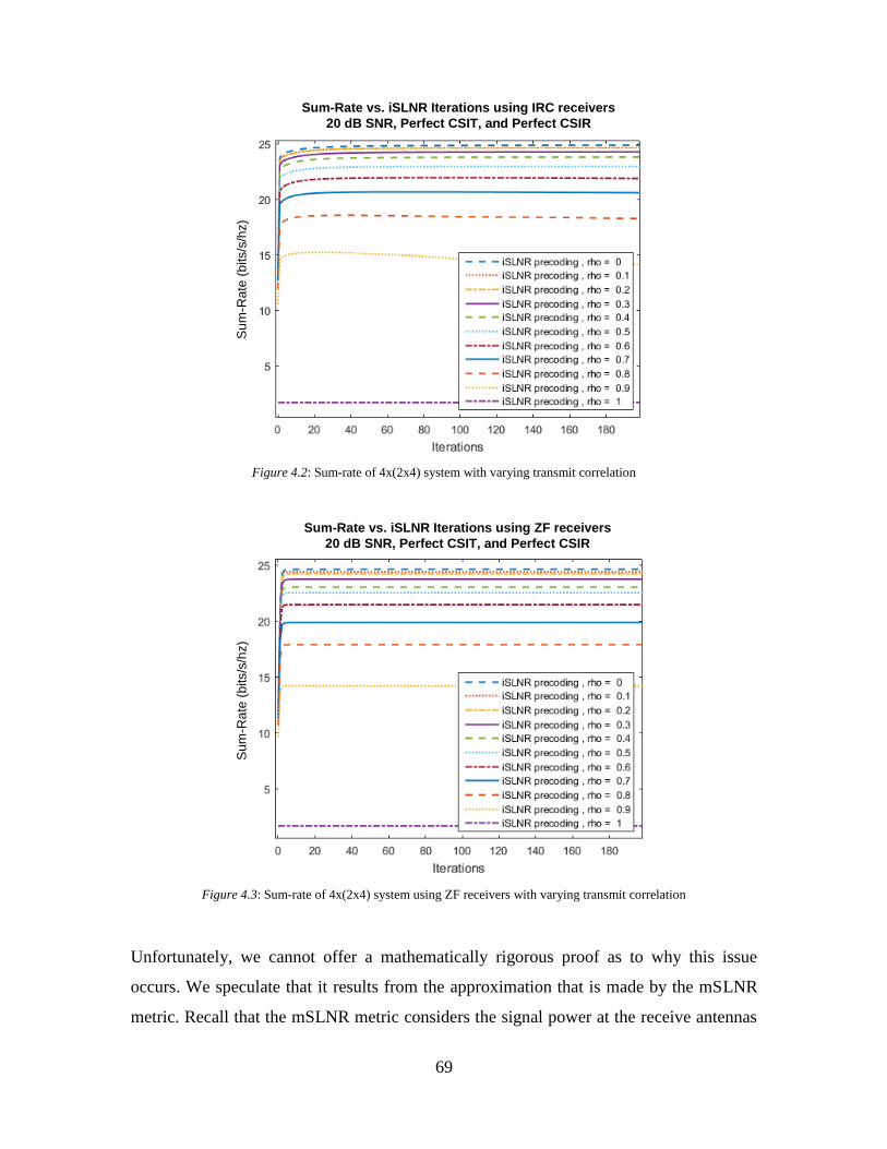
69


Figure 4.3: Sum-rate of 4x(2x4) system using ZF receivers with varying transmit correlation

Unfortunately, we cannot offer a mathematically rigorous proof as to why this issue

occurs. We speculate that it results from the approximation that is made by the mSLNR

metric. Recall that the mSLNR metric considers the signal power at the receive antennas



Su

m-R

ate

(b

its/s

/hz)

Sum-Rate vs. iSLNR Iterations using ZF receivers


Su

m-R

ate

(b

its/s

/hz)

70

but the noise and leakage are considered after the receiver processing. There is no

guarantee that maximizing this metric will in fact maximize the SINR at the output of the

receiver. In most cases simulations have shown that it will, but it appears that the

approximation may break down with high transmit antenna correlation and IRC receivers.

From what we’ve seen, even in this case the algorithm will provide a substantial initial

gain.

In this section we investigated the impact of transmit antenna correlation on the achieved

sum-rate using the iSLNR algorithm. We first observed that increased transmit antenna

correlation will degrade the system sum-rate. We further observed that the iSLNR

algorithm will consistently provide gain in system sum-rate with two caveats: (1) no

observable gain is achieved when the transmit antennas are perfectly correlated and (2)

the gain provided may not be monotonically increasing per iteration with high transmit

antenna correlation. From our simulations the latter caveat appears to be limited to the

case where IRC receivers are used and is most prominent when 𝑁 < ∑𝑀𝑖.

4.2 Time-Varying Channels

So far we have assumed a static channel for the duration of each transmission. While this

is useful to compare the effect of imperfect CSIT and CSIR, and indeed may be a

reasonable approximation in low-mobility scenarios, real world systems will often exhibit

time-variance in the channel due to user mobility and/or changes in the environment. It is

therefore worthwhile to consider how this will affect the system. In a time-varying

channel, the quality of CSIT will degrade over time, though the CSIR will track the

changes. Time-varying channels are therefore a natural extension of the previously

described iSLNR algorithm considering CSIT error.

In this work we use Jake’s model for narrowband time-varying channels. Jake’s model

assumes some number (typically around 50) of multi-path scatterers with angles-of-arrival

that are uniformly distributed around the antennas and which have experienced Doppler

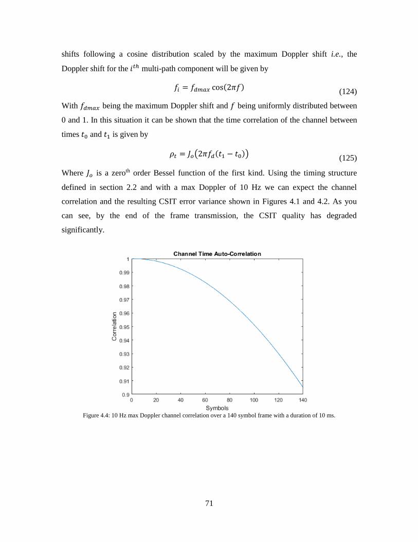
71

shifts following a cosine distribution scaled by the maximum Doppler shift i.e., the

Doppler shift for the 𝑖𝑡ℎ multi-path component will be given by

𝑓𝑖 = 𝑓𝑑𝑚𝑎𝑥 cos(2𝜋𝑓) (124)

With 𝑓𝑑𝑚𝑎𝑥 being the maximum Doppler shift and 𝑓 being uniformly distributed between

0 and 1. In this situation it can be shown that the time correlation of the channel between

times 𝑡0 and 𝑡1 is given by

𝜌𝑡 = 𝐽𝑜(2𝜋𝑓𝑑(𝑡1 − 𝑡0)) (125)

Where 𝐽𝑜 is a zeroth order Bessel function of the first kind. Using the timing structure

defined in section 2.2 and with a max Doppler of 10 Hz we can expect the channel

correlation and the resulting CSIT error variance shown in Figures 4.1 and 4.2. As you

can see, by the end of the frame transmission, the CSIT quality has degraded

significantly.

Figure 4.4: 10 Hz max Doppler channel correlation over a 140 symbol frame with a duration of 10 ms.

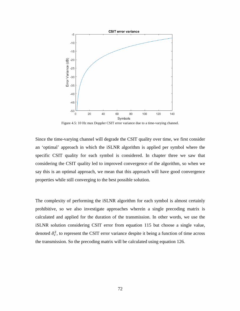
72

Figure 4.5: 10 Hz max Doppler CSIT error variance due to a time-varying channel.

Since the time-varying channel will degrade the CSIT quality over time, we first consider

an ‘optimal’ approach in which the iSLNR algorithm is applied per symbol where the

specific CSIT quality for each symbol is considered. In chapter three we saw that

considering the CSIT quality led to improved convergence of the algorithm, so when we

say this is an optimal approach, we mean that this approach will have good convergence

properties while still converging to the best possible solution.

The complexity of performing the iSLNR algorithm for each symbol is almost certainly

prohibitive, so we also investigate approaches wherein a single precoding matrix is

calculated and applied for the duration of the transmission. In other words, we use the

iSLNR solution considering CSIT error from equation 115 but choose a single value,

denoted �̂�𝑐2, to represent the CSIT error variance despite it being a function of time across

the transmission. So the precoding matrix will be calculated using equation 126.

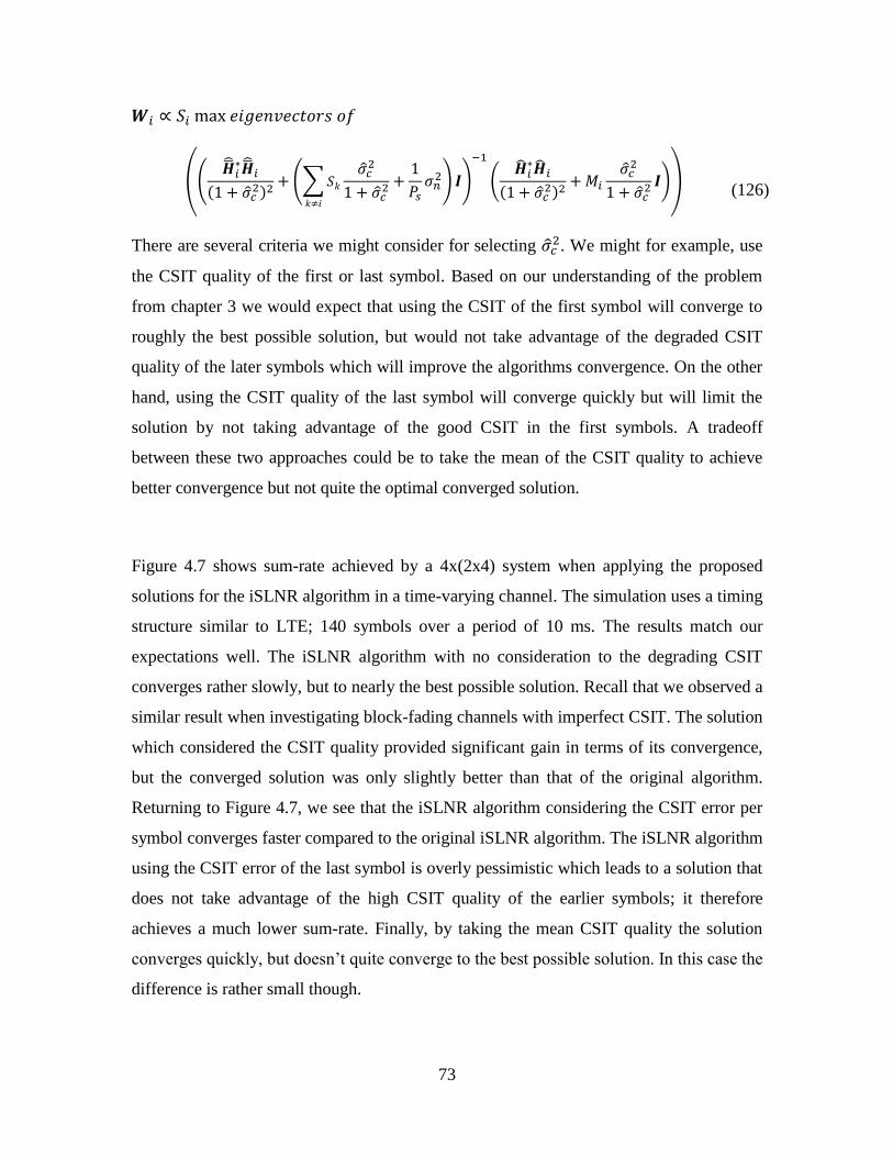
73


((�̂̅�𝑖

∗�̂̅�𝑖

(1 + �̂�𝑐2)2

+ (∑ 𝑆𝑘

𝑘≠𝑖

�̂�𝑐2

1 + �̂�𝑐2 +

1

𝑃𝑠𝜎𝑛

2) 𝑰)

−1

(�̂�𝑖

∗�̂�𝑖

(1 + �̂�𝑐2)2

+ 𝑀𝑖

�̂�𝑐2

1 + �̂�𝑐2 𝑰))

(126)

There are several criteria we might consider for selecting �̂�𝑐2. We might for example, use

the CSIT quality of the first or last symbol. Based on our understanding of the problem

from chapter 3 we would expect that using the CSIT of the first symbol will converge to

roughly the best possible solution, but would not take advantage of the degraded CSIT

quality of the later symbols which will improve the algorithms convergence. On the other

hand, using the CSIT quality of the last symbol will converge quickly but will limit the

solution by not taking advantage of the good CSIT in the first symbols. A tradeoff

between these two approaches could be to take the mean of the CSIT quality to achieve

better convergence but not quite the optimal converged solution.

Figure 4.7 shows sum-rate achieved by a 4x(2x4) system when applying the proposed

solutions for the iSLNR algorithm in a time-varying channel. The simulation uses a timing

structure similar to LTE; 140 symbols over a period of 10 ms. The results match our

expectations well. The iSLNR algorithm with no consideration to the degrading CSIT

converges rather slowly, but to nearly the best possible solution. Recall that we observed a

similar result when investigating block-fading channels with imperfect CSIT. The solution

which considered the CSIT quality provided significant gain in terms of its convergence,

but the converged solution was only slightly better than that of the original algorithm.

Returning to Figure 4.7, we see that the iSLNR algorithm considering the CSIT error per

symbol converges faster compared to the original iSLNR algorithm. The iSLNR algorithm

using the CSIT error of the last symbol is overly pessimistic which leads to a solution that

does not take advantage of the high CSIT quality of the earlier symbols; it therefore

achieves a much lower sum-rate. Finally, by taking the mean CSIT quality the solution

converges quickly, but doesn’t quite converge to the best possible solution. In this case the

difference is rather small though.

74

Figure 4.6: Sum-rate of a 4x(2x4) system in a time-varying channel

Figure 4.8 shows similar results for a 16x(2x8) system when applying the proposed

solutions for the iSLNR algorithm in a time-varying channel. In this case the differences

are more pronounced. Using the CSIT quality based on the last symbol severely limits the

achieved sum-rate. Even using the mean limits the solution non-trivially. Using the per-

symbol precoding provides a nice improvement in convergence while achieving a solution

slightly better than the single solution with no consideration to the degrading CSIT.



Su

m-R

ate

(b

its/s

/hz)

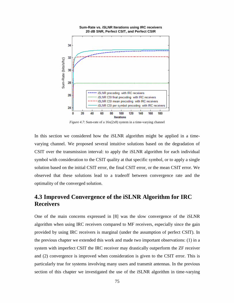
75

Figure 4.7: Sum-rate of a 16x(2x8) system in a time-varying channel

In this section we considered how the iSLNR algorithm might be applied in a time-

varying channel. We proposed several intuitive solutions based on the degradation of

CSIT over the transmission interval: to apply the iSLNR algorithm for each individual

symbol with consideration to the CSIT quality at that specific symbol, or to apply a single

solution based on the initial CSIT error, the final CSIT error, or the mean CSIT error. We

observed that these solutions lead to a tradeoff between convergence rate and the

optimality of the converged solution.

4.3 Improved Convergence of the iSLNR Algorithm for IRC

Receivers

One of the main concerns expressed in [8] was the slow convergence of the iSLNR

algorithm when using IRC receivers compared to MF receivers, especially since the gain

provided by using IRC receivers is marginal (under the assumption of perfect CSIT). In

the previous chapter we extended this work and made two important observations: (1) in a

system with imperfect CSIT the IRC receiver may drastically outperform the ZF receiver

and (2) convergence is improved when consideration is given to the CSIT error. This is

particularly true for systems involving many users and transmit antennas. In the previous

section of this chapter we investigated the use of the iSLNR algorithm in time-varying



Su

m-R

ate

(b

its/s

/hz)

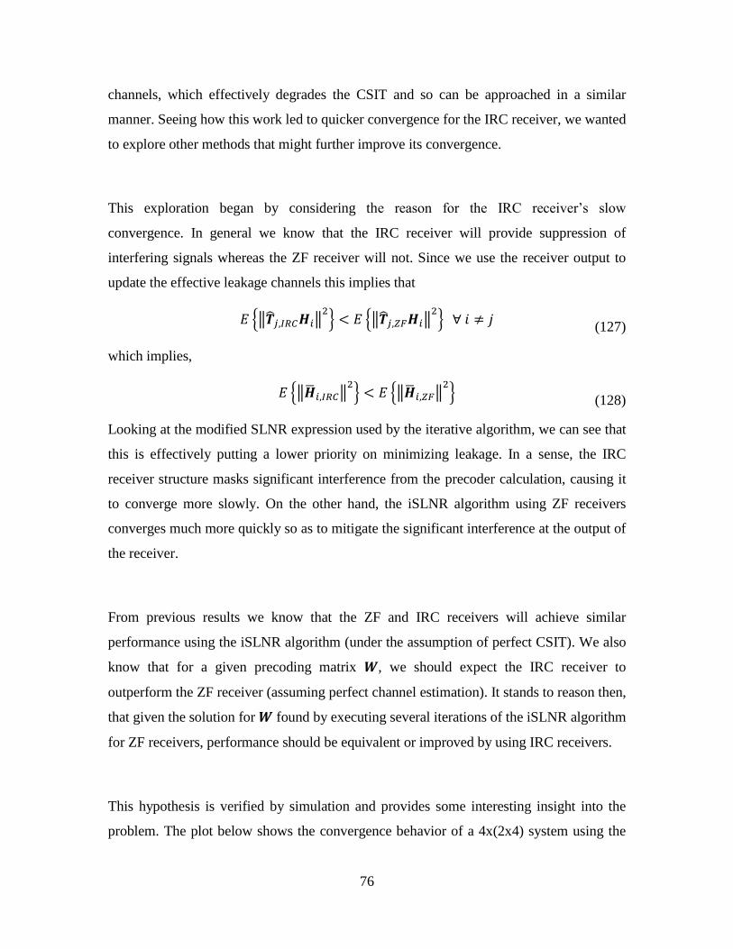
76

channels, which effectively degrades the CSIT and so can be approached in a similar

manner. Seeing how this work led to quicker convergence for the IRC receiver, we wanted

to explore other methods that might further improve its convergence.

This exploration began by considering the reason for the IRC receiver’s slow

convergence. In general we know that the IRC receiver will provide suppression of

interfering signals whereas the ZF receiver will not. Since we use the receiver output to

update the effective leakage channels this implies that

𝐸 {‖�̂�𝑗,𝐼𝑅𝐶𝑯𝑖‖2} < 𝐸 {‖�̂�𝑗,𝑍𝐹𝑯𝑖‖

2} ∀ 𝑖 ≠ 𝑗

(127)

which implies,

𝐸 {‖�̅�𝑖,𝐼𝑅𝐶‖2} < 𝐸 {‖�̅�𝑖,𝑍𝐹‖

2}

(128)

Looking at the modified SLNR expression used by the iterative algorithm, we can see that

this is effectively putting a lower priority on minimizing leakage. In a sense, the IRC

receiver structure masks significant interference from the precoder calculation, causing it

to converge more slowly. On the other hand, the iSLNR algorithm using ZF receivers

converges much more quickly so as to mitigate the significant interference at the output of

the receiver.

From previous results we know that the ZF and IRC receivers will achieve similar

performance using the iSLNR algorithm (under the assumption of perfect CSIT). We also

know that for a given precoding matrix 𝑾, we should expect the IRC receiver to

outperform the ZF receiver (assuming perfect channel estimation). It stands to reason then,

that given the solution for 𝑾 found by executing several iterations of the iSLNR algorithm

for ZF receivers, performance should be equivalent or improved by using IRC receivers.

This hypothesis is verified by simulation and provides some interesting insight into the

problem. The plot below shows the convergence behavior of a 4x(2x4) system using the

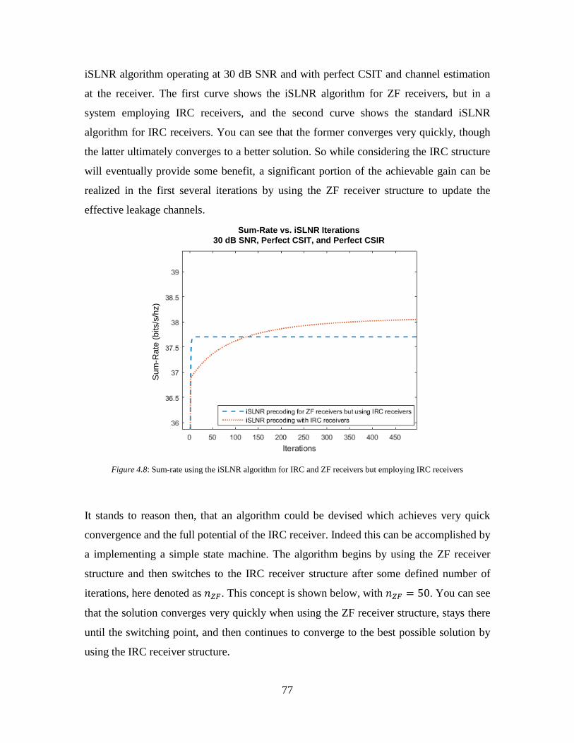
77

iSLNR algorithm operating at 30 dB SNR and with perfect CSIT and channel estimation

at the receiver. The first curve shows the iSLNR algorithm for ZF receivers, but in a

system employing IRC receivers, and the second curve shows the standard iSLNR

algorithm for IRC receivers. You can see that the former converges very quickly, though

the latter ultimately converges to a better solution. So while considering the IRC structure

will eventually provide some benefit, a significant portion of the achievable gain can be

realized in the first several iterations by using the ZF receiver structure to update the

effective leakage channels.

Figure 4.8: Sum-rate using the iSLNR algorithm for IRC and ZF receivers but employing IRC receivers

It stands to reason then, that an algorithm could be devised which achieves very quick

convergence and the full potential of the IRC receiver. Indeed this can be accomplished by

a implementing a simple state machine. The algorithm begins by using the ZF receiver

structure and then switches to the IRC receiver structure after some defined number of

iterations, here denoted as 𝑛𝑍𝐹. This concept is shown below, with 𝑛𝑍𝐹 = 50. You can see

that the solution converges very quickly when using the ZF receiver structure, stays there

until the switching point, and then continues to converge to the best possible solution by

using the IRC receiver structure.



Su

m-R

ate

(b

its/s

/hz)

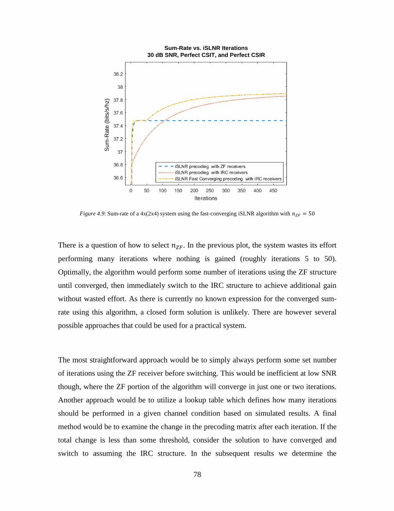
78

Figure 4.9: Sum-rate of a 4x(2x4) system using the fast-converging iSLNR algorithm with 𝑛𝑍𝐹 = 50

There is a question of how to select 𝑛𝑍𝐹. In the previous plot, the system wastes its effort

performing many iterations where nothing is gained (roughly iterations 5 to 50).

Optimally, the algorithm would perform some number of iterations using the ZF structure

until converged, then immediately switch to the IRC structure to achieve additional gain

without wasted effort. As there is currently no known expression for the converged sum-

rate using this algorithm, a closed form solution is unlikely. There are however several

possible approaches that could be used for a practical system.

The most straightforward approach would be to simply always perform some set number

of iterations using the ZF receiver before switching. This would be inefficient at low SNR

though, where the ZF portion of the algorithm will converge in just one or two iterations.

Another approach would be to utilize a lookup table which defines how many iterations

should be performed in a given channel condition based on simulated results. A final

method would be to examine the change in the precoding matrix after each iteration. If the

total change is less than some threshold, consider the solution to have converged and

switch to assuming the IRC structure. In the subsequent results we determine the



Su

m-R

ate

(b

its/s

/hz)

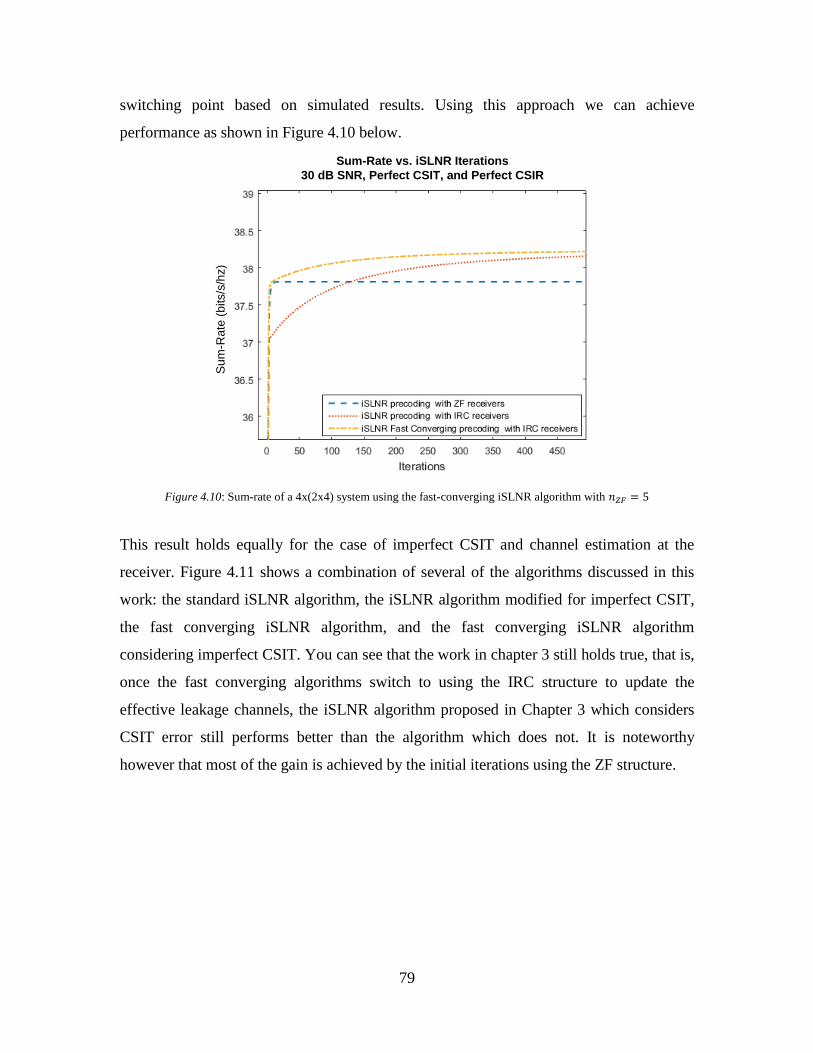
79

switching point based on simulated results. Using this approach we can achieve

performance as shown in Figure 4.10 below.

Figure 4.10: Sum-rate of a 4x(2x4) system using the fast-converging iSLNR algorithm with 𝑛𝑍𝐹 = 5

This result holds equally for the case of imperfect CSIT and channel estimation at the

receiver. Figure 4.11 shows a combination of several of the algorithms discussed in this

work: the standard iSLNR algorithm, the iSLNR algorithm modified for imperfect CSIT,

the fast converging iSLNR algorithm, and the fast converging iSLNR algorithm

considering imperfect CSIT. You can see that the work in chapter 3 still holds true, that is,

once the fast converging algorithms switch to using the IRC structure to update the

effective leakage channels, the iSLNR algorithm proposed in Chapter 3 which considers

CSIT error still performs better than the algorithm which does not. It is noteworthy

however that most of the gain is achieved by the initial iterations using the ZF structure.



Su

m-R

ate

(b

its/s

/hz)

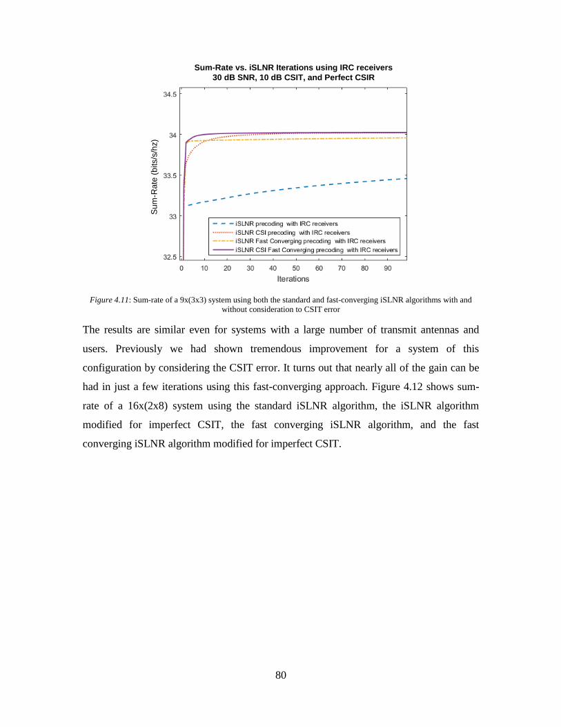
80

Figure 4.11: Sum-rate of a 9x(3x3) system using both the standard and fast-converging iSLNR algorithms with and

without consideration to CSIT error

The results are similar even for systems with a large number of transmit antennas and

users. Previously we had shown tremendous improvement for a system of this

configuration by considering the CSIT error. It turns out that nearly all of the gain can be

had in just a few iterations using this fast-converging approach. Figure 4.12 shows sum-

rate of a 16x(2x8) system using the standard iSLNR algorithm, the iSLNR algorithm

modified for imperfect CSIT, the fast converging iSLNR algorithm, and the fast

converging iSLNR algorithm modified for imperfect CSIT.



Su

m-R

ate

(b

its/s

/hz)

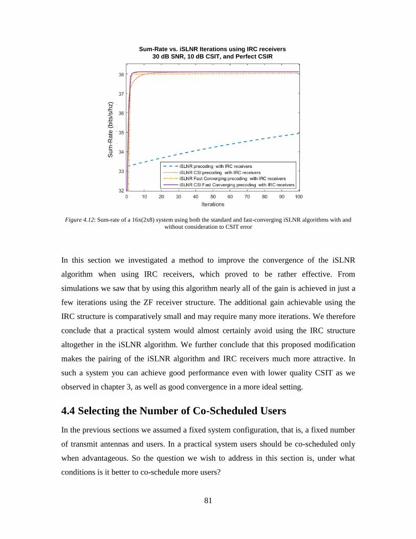
81

Figure 4.12: Sum-rate of a 16x(2x8) system using both the standard and fast-converging iSLNR algorithms with and

without consideration to CSIT error

In this section we investigated a method to improve the convergence of the iSLNR

algorithm when using IRC receivers, which proved to be rather effective. From

simulations we saw that by using this algorithm nearly all of the gain is achieved in just a

few iterations using the ZF receiver structure. The additional gain achievable using the

IRC structure is comparatively small and may require many more iterations. We therefore

conclude that a practical system would almost certainly avoid using the IRC structure

altogether in the iSLNR algorithm. We further conclude that this proposed modification

makes the pairing of the iSLNR algorithm and IRC receivers much more attractive. In

such a system you can achieve good performance even with lower quality CSIT as we

observed in chapter 3, as well as good convergence in a more ideal setting.

4.4 Selecting the Number of Co-Scheduled Users

In the previous sections we assumed a fixed system configuration, that is, a fixed number

of transmit antennas and users. In a practical system users should be co-scheduled only

when advantageous. So the question we wish to address in this section is, under what

conditions is it better to co-schedule more users?



Su

m-R

ate

(b

its/s

/hz)

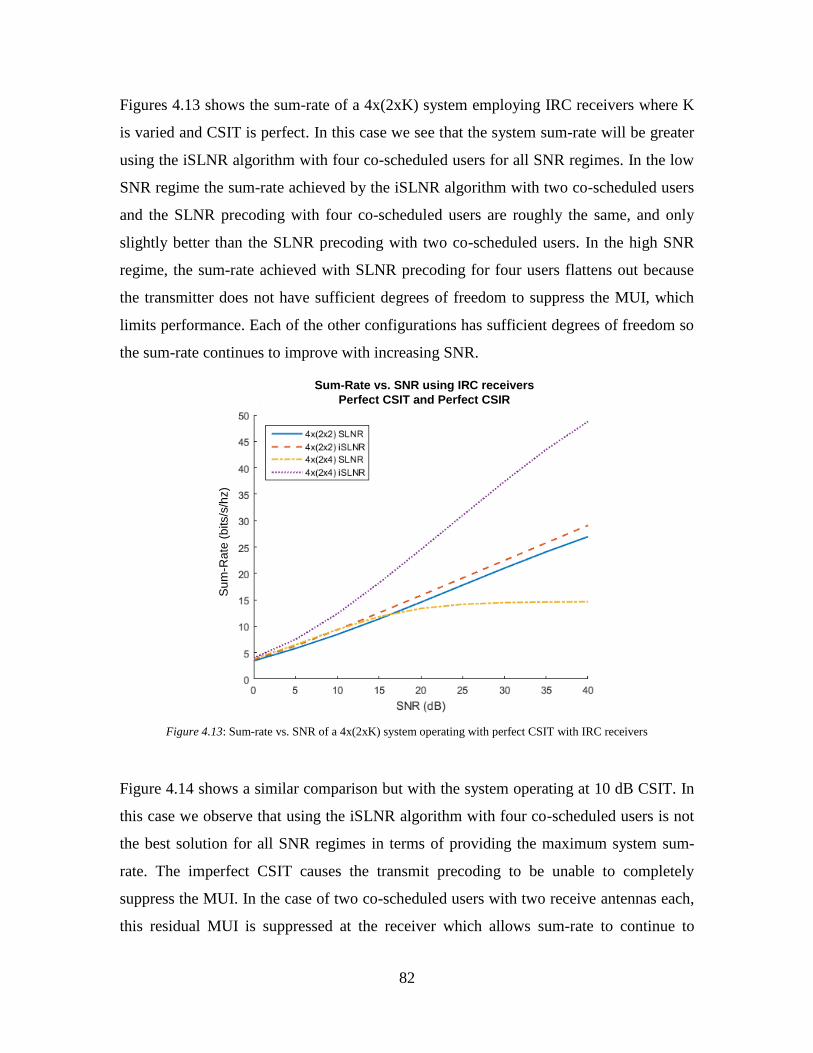
82

Figures 4.13 shows the sum-rate of a 4x(2xK) system employing IRC receivers where K

is varied and CSIT is perfect. In this case we see that the system sum-rate will be greater

using the iSLNR algorithm with four co-scheduled users for all SNR regimes. In the low

SNR regime the sum-rate achieved by the iSLNR algorithm with two co-scheduled users

and the SLNR precoding with four co-scheduled users are roughly the same, and only

slightly better than the SLNR precoding with two co-scheduled users. In the high SNR

regime, the sum-rate achieved with SLNR precoding for four users flattens out because

the transmitter does not have sufficient degrees of freedom to suppress the MUI, which

limits performance. Each of the other configurations has sufficient degrees of freedom so

the sum-rate continues to improve with increasing SNR.

Figure 4.13: Sum-rate vs. SNR of a 4x(2xK) system operating with perfect CSIT with IRC receivers

Figure 4.14 shows a similar comparison but with the system operating at 10 dB CSIT. In

this case we observe that using the iSLNR algorithm with four co-scheduled users is not

the best solution for all SNR regimes in terms of providing the maximum system sum-

rate. The imperfect CSIT causes the transmit precoding to be unable to completely

suppress the MUI. In the case of two co-scheduled users with two receive antennas each,

this residual MUI is suppressed at the receiver which allows sum-rate to continue to

Sum-Rate vs. SNR using IRC receivers

Perfect CSIT and Perfect CSIR

Su

m-R

ate

(b

its/s

/hz)

83

improve at high SNR. On the other hand with four co-scheduled users each with two

receive antennas the residual MUI cannot be fully suppressed at the receiver. This causes

the achievable sum-rate to flatten out in the high SNR regime. We observe however that

in the low SNR regime the residual MUI is not the dominant impairment, so having more

users leads to improved sum-rate. So we see that the CSIT quality should be considered

when deciding how many users are to be co-scheduled.

Figure 4.14: Sum-rate vs. SNR of a 4x(2xK) system operating with 10 dB CSIT with IRC receivers

Figure 4.15 shows a 4x(2xK) system employing ZF receivers operating at 10 dB CSIT.

Note that in this case the receivers are unable to suppress the residual MUI. This means

that the sum-rate will reach a maximum even for the two user case. So we observe that

with ZF receivers the system sum-rate will always be best by using the iSLNR algorithm

with four users.


10 dB CSIT, and Perfect CSIR

Su

m-R

ate

(b

its/s

/hz)

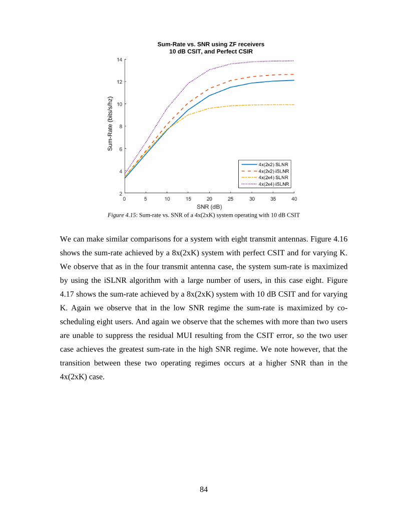
84

Figure 4.15: Sum-rate vs. SNR of a 4x(2xK) system operating with 10 dB CSIT

We can make similar comparisons for a system with eight transmit antennas. Figure 4.16

shows the sum-rate achieved by a 8x(2xK) system with perfect CSIT and for varying K.

We observe that as in the four transmit antenna case, the system sum-rate is maximized

by using the iSLNR algorithm with a large number of users, in this case eight. Figure

4.17 shows the sum-rate achieved by a 8x(2xK) system with 10 dB CSIT and for varying

K. Again we observe that in the low SNR regime the sum-rate is maximized by co-

scheduling eight users. And again we observe that the schemes with more than two users

are unable to suppress the residual MUI resulting from the CSIT error, so the two user

case achieves the greatest sum-rate in the high SNR regime. We note however, that the

transition between these two operating regimes occurs at a higher SNR than in the

4x(2xK) case.

Sum-Rate vs. SNR using ZF receivers


Su

m-R

ate

(b

its/s

/hz)

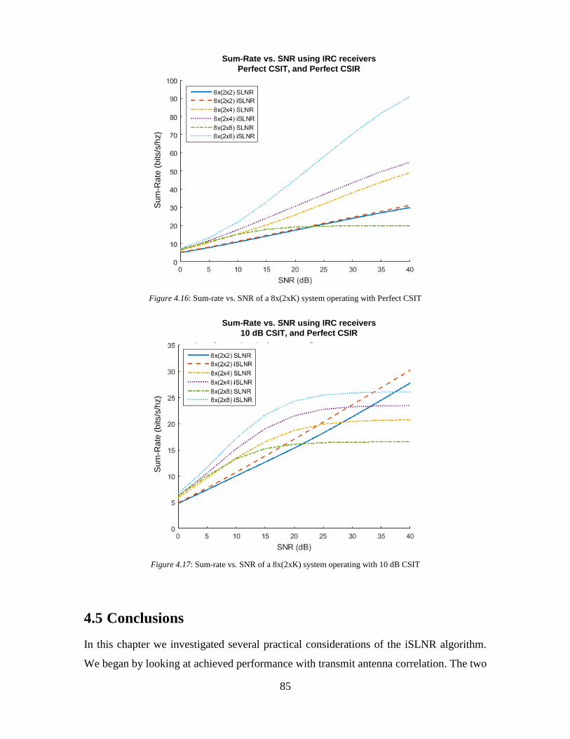
85

Figure 4.16: Sum-rate vs. SNR of a 8x(2xK) system operating with Perfect CSIT

Figure 4.17: Sum-rate vs. SNR of a 8x(2xK) system operating with 10 dB CSIT

4.5 Conclusions

In this chapter we investigated several practical considerations of the iSLNR algorithm.

We began by looking at achieved performance with transmit antenna correlation. The two


Perfect CSIT, and Perfect CSIR

Su

m-R

ate

(b

its/s

/hz)



Su

m-R

ate

(b

its/s

/hz)

86

key observations were as follows: (1) system sum-rate decreases with increased transmit

antenna correlation and (2) sum-rate may not be monotonically increasing per iteration of

the algorithm when transmit antenna correlation is high and IRC receivers are used. We

continued by examining performance of the iSLNR algorithm in time-varying channels

using several possible approaches based on our previous analysis on imperfect CSIT. We

showed that there is an inherent tradeoff between achieving fast convergence and

achieving the best possible converged solution. We then proposed a modification to the

algorithm which can drastically improve its convergence when IRC receivers are

employed. It was shown that using this approach coupled with the solution which

considers CSIT error provides the best convergence. With this modification in mind the

advantage of the IRC receiver is clear as it will achieve the same performance as the ZF

receiver even at just a few iterations in ideal conditions besides also achieving

significantly better performance with imperfect CSIT as we saw in the previous chapter.

Finally, we examined the sum-rate achieved by a system with a fixed number of transmit

antennas but with a varied number of co-scheduled users and operating with various

qualities of CSIT. From this work we observed that in the ideal case it is always best to

co-schedule the maximum number of users supported by the degrees of freedom achieved

with the iSLNR algorithm, but with imperfect CSIT the number of users which will

maximize the system sum-rate may depend on the SNR. At low SNR it is best to co-

schedule the maximum number of users with the iSLNR algorithm, but at high SNR the

imperfect CSIT causes residual MUI which dominates performance, making it better to

co-schedule fewer users.

87

Chapter 5

iSLNR for LTE-A

In this chapter we demonstrate the application of the iSLNR algorithm to one of the most

prominent modern day wireless standards, LTE-A. There are several key distinctions

between the previous analysis and an implementation for LTE-A which will be discussed

later. In the first section of this chapter we provide the necessary background on the LTE-

A standard. The second section presents the simulated performance of the algorithm, and

finally we draw conclusions on the utility of the iSLNR algorithm for LTE-A.

5.1 MU-MIMO in LTE-A

In this section we go over the details of the implementation of MU-MIMO in LTE-A.

Specifically, we desire to understand how the waveforms are modulated, how precoding

is accomplished at the base station, how channel estimation may be performed at the user,

and how these considerations may impact the iSLNR algorithm.

5.1.1 Downlink Waveform

The LTE-A downlink uses orthogonal frequency division multiplexing (OFDM), wherein

many narrowband carriers are transmitted in parallel. This provides several nice features:

(1) each subcarrier experiences frequency flat fading (2) inter-symbol-interference can be

mitigated by the insertion of a cyclic-prefix and (3) the FFT and IFFT provide efficient

means of implementing the OFDM modem in hardware/software. Precoding can be

performed simply by multiplying each symbol by the precoding weights prior to the IFFT

operation. A block diagram of a MIMO-OFDM system is included below in Figure 5.1.

In this case there is only one user.

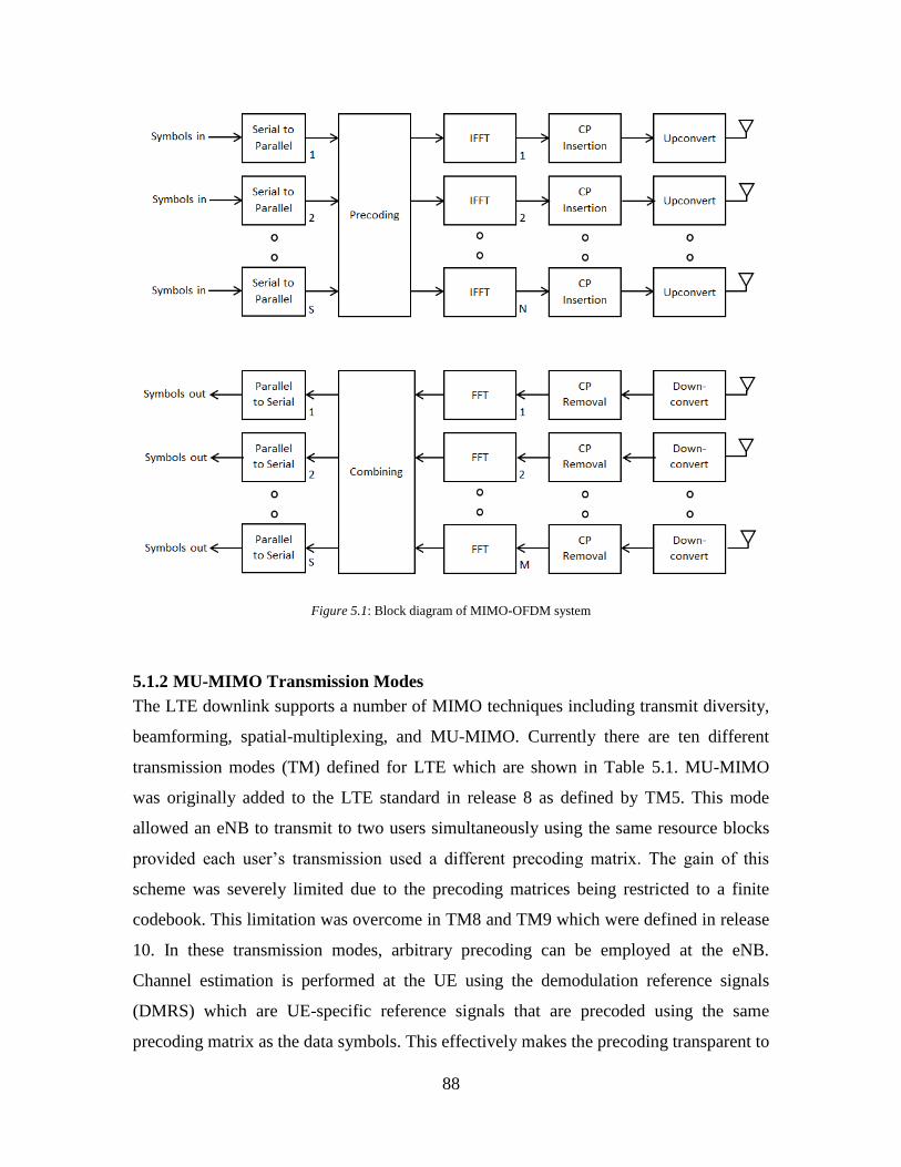
88

Figure 5.1: Block diagram of MIMO-OFDM system

5.1.2 MU-MIMO Transmission Modes

The LTE downlink supports a number of MIMO techniques including transmit diversity,

beamforming, spatial-multiplexing, and MU-MIMO. Currently there are ten different

transmission modes (TM) defined for LTE which are shown in Table 5.1. MU-MIMO

was originally added to the LTE standard in release 8 as defined by TM5. This mode

allowed an eNB to transmit to two users simultaneously using the same resource blocks

provided each user’s transmission used a different precoding matrix. The gain of this

scheme was severely limited due to the precoding matrices being restricted to a finite

codebook. This limitation was overcome in TM8 and TM9 which were defined in release

10. In these transmission modes, arbitrary precoding can be employed at the eNB.

Channel estimation is performed at the UE using the demodulation reference signals

(DMRS) which are UE-specific reference signals that are precoded using the same

precoding matrix as the data symbols. This effectively makes the precoding transparent to

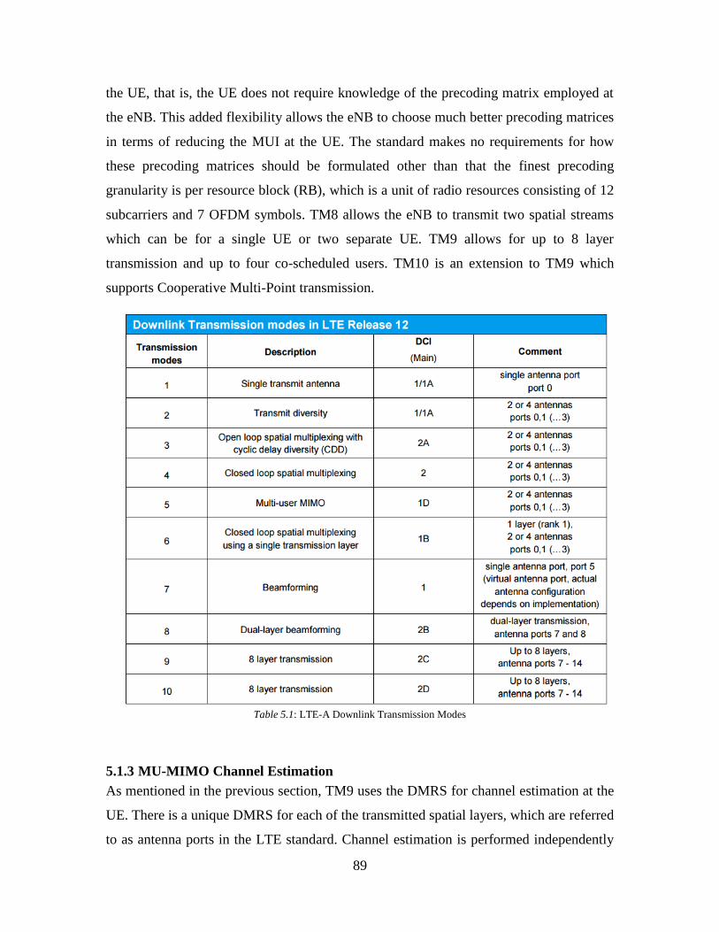
89

the UE, that is, the UE does not require knowledge of the precoding matrix employed at

the eNB. This added flexibility allows the eNB to choose much better precoding matrices

in terms of reducing the MUI at the UE. The standard makes no requirements for how

these precoding matrices should be formulated other than that the finest precoding

granularity is per resource block (RB), which is a unit of radio resources consisting of 12

subcarriers and 7 OFDM symbols. TM8 allows the eNB to transmit two spatial streams

which can be for a single UE or two separate UE. TM9 allows for up to 8 layer

transmission and up to four co-scheduled users. TM10 is an extension to TM9 which

supports Cooperative Multi-Point transmission.

Table 5.1: LTE-A Downlink Transmission Modes

5.1.3 MU-MIMO Channel Estimation

As mentioned in the previous section, TM9 uses the DMRS for channel estimation at the

UE. There is a unique DMRS for each of the transmitted spatial layers, which are referred

to as antenna ports in the LTE standard. Channel estimation is performed independently

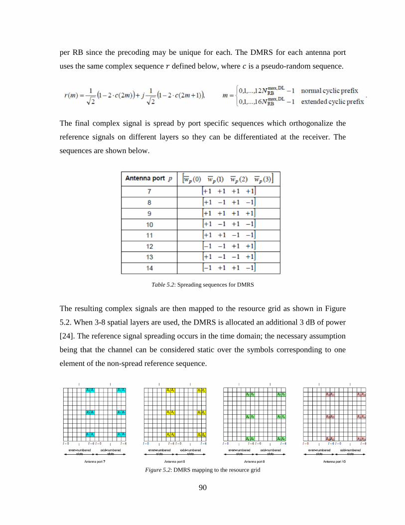
90

per RB since the precoding may be unique for each. The DMRS for each antenna port

uses the same complex sequence 𝑟 defined below, where 𝑐 is a pseudo-random sequence.

The final complex signal is spread by port specific sequences which orthogonalize the

reference signals on different layers so they can be differentiated at the receiver. The

sequences are shown below.

Table 5.2: Spreading sequences for DMRS

The resulting complex signals are then mapped to the resource grid as shown in Figure

5.2. When 3-8 spatial layers are used, the DMRS is allocated an additional 3 dB of power

[24]. The reference signal spreading occurs in the time domain; the necessary assumption

being that the channel can be considered static over the symbols corresponding to one

element of the non-spread reference sequence.

Figure 5.2: DMRS mapping to the resource grid

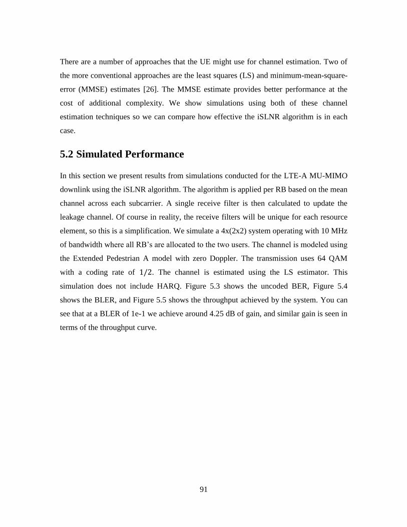
91

There are a number of approaches that the UE might use for channel estimation. Two of

the more conventional approaches are the least squares (LS) and minimum-mean-square-

error (MMSE) estimates [26]. The MMSE estimate provides better performance at the

cost of additional complexity. We show simulations using both of these channel

estimation techniques so we can compare how effective the iSLNR algorithm is in each

case.

5.2 Simulated Performance

In this section we present results from simulations conducted for the LTE-A MU-MIMO

downlink using the iSLNR algorithm. The algorithm is applied per RB based on the mean

channel across each subcarrier. A single receive filter is then calculated to update the

leakage channel. Of course in reality, the receive filters will be unique for each resource

element, so this is a simplification. We simulate a 4x(2x2) system operating with 10 MHz

of bandwidth where all RB’s are allocated to the two users. The channel is modeled using

the Extended Pedestrian A model with zero Doppler. The transmission uses 64 QAM

with a coding rate of 1/2. The channel is estimated using the LS estimator. This

simulation does not include HARQ. Figure 5.3 shows the uncoded BER, Figure 5.4

shows the BLER, and Figure 5.5 shows the throughput achieved by the system. You can

see that at a BLER of 1e-1 we achieve around 4.25 dB of gain, and similar gain is seen in

terms of the throughput curve.

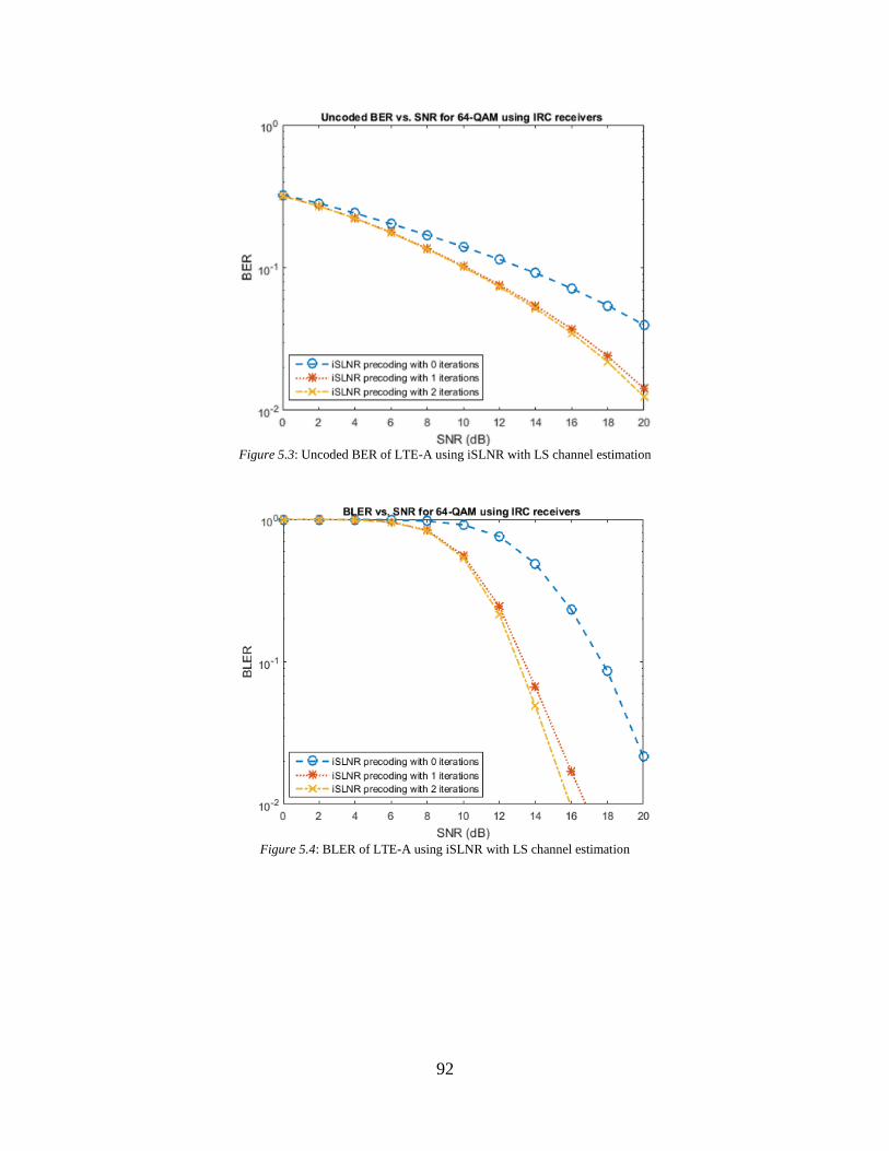
92

Figure 5.3: Uncoded BER of LTE-A using iSLNR with LS channel estimation

Figure 5.4: BLER of LTE-A using iSLNR with LS channel estimation

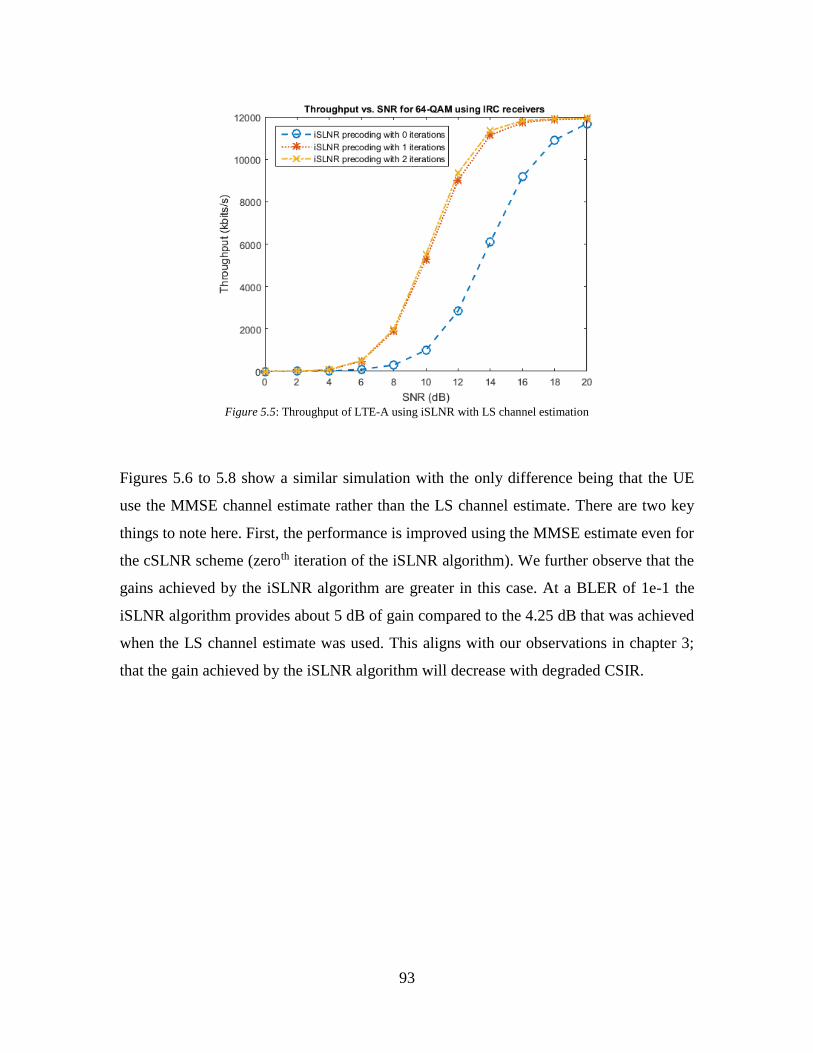
93

Figure 5.5: Throughput of LTE-A using iSLNR with LS channel estimation

Figures 5.6 to 5.8 show a similar simulation with the only difference being that the UE

use the MMSE channel estimate rather than the LS channel estimate. There are two key

things to note here. First, the performance is improved using the MMSE estimate even for

the cSLNR scheme (zeroth iteration of the iSLNR algorithm). We further observe that the

gains achieved by the iSLNR algorithm are greater in this case. At a BLER of 1e-1 the

iSLNR algorithm provides about 5 dB of gain compared to the 4.25 dB that was achieved

when the LS channel estimate was used. This aligns with our observations in chapter 3;

that the gain achieved by the iSLNR algorithm will decrease with degraded CSIR.

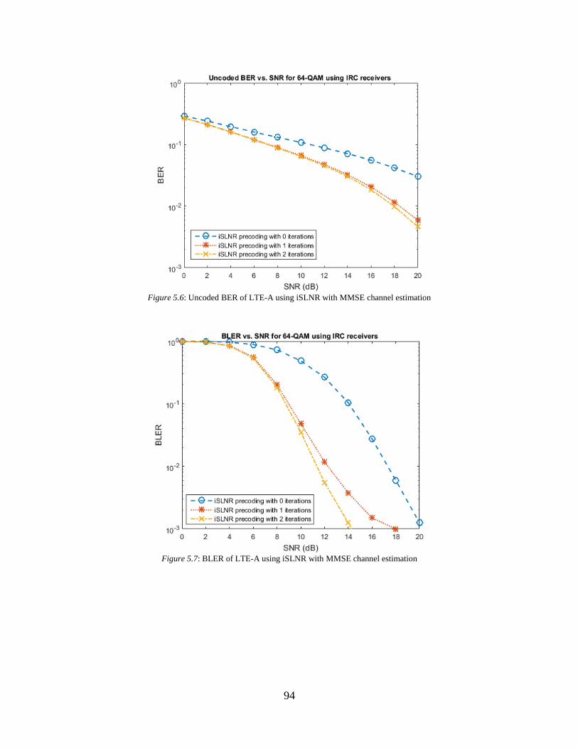
94

Figure 5.6: Uncoded BER of LTE-A using iSLNR with MMSE channel estimation

Figure 5.7: BLER of LTE-A using iSLNR with MMSE channel estimation

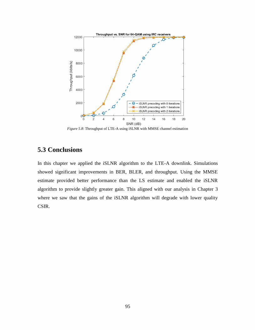
95

Figure 5.8: Throughput of LTE-A using iSLNR with MMSE channel estimation

5.3 Conclusions

In this chapter we applied the iSLNR algorithm to the LTE-A downlink. Simulations

showed significant improvements in BER, BLER, and throughput. Using the MMSE

estimate provided better performance than the LS estimate and enabled the iSLNR

algorithm to provide slightly greater gain. This aligned with our analysis in Chapter 3

where we saw that the gains of the iSLNR algorithm will degrade with lower quality

CSIR.

96

Chapter 6

Conclusion

In this thesis we have examined a number of practical aspects of leakage-based precoding

for the MU-MIMO downlink. We began by considering the impact of imperfect CSIT

and proposing solutions which mitigate the performance degradation. We also

investigated the impact of imperfect CSIR. We then continued by examining the impact

of other practical considerations such as transmit antenna correlation and time-varying

channels. We also proposed a simple modification which can improve convergence of the

algorithm with IRC receivers and examined the problem of selecting the number of co-

scheduled users. Finally, we demonstrated performance of the algorithm when applied to

the LTE-A framework for MU-MIMO.

Our analysis of imperfect CSI began by deriving an expression for the precoding matrices

which will maximize the SLNR in the presence of imperfect CSIT. Simulations showed

that the derived solution was superior to the one previously proposed in [7] which used

the same error model. We then went on to examine the impact of modifying the CSIT to

meet the MMSE criteria without relying on knowledge of the true channel as in [12]. This

showed a marginal though non-negligible performance gain for the cSLNR precoding

scheme. Next, we applied similar analysis to the iSLNR algorithm. The derivation of the

precoding solution follows the same approach as with the cSLNR scheme, but we also

had to consider the effect that the CSIT error had on the receive filter calculations.

Simulations showed that the proposed solutions can provide substantial gains compared

to the iSLNR algorithm which does not consider imperfect CSIT. We also observed that

with imperfect CSIT, the sum-rate achieved with IRC receivers can be much greater than

that achieved with ZF receivers. We then investigated the same MMSE modification for

the iSLNR algorithm and found that after several iterations the gain had become

negligible. We also showed the performance degradation due to imperfect CSIR. It was

shown that the CSIR quality must be sufficiently high for the iSLNR algorithm to provide

substantial performance gains.

97

Through simulation we demonstrated the performance degradations experienced due to

transmit antenna correlation and time-varying channels. We observed that the sum-rate

achieved using the iSLNR algorithm may not be monotonically increasing per iteration

when IRC receivers are used and transmit antenna correlation is high. We demonstrated

how our work on imperfect CSIT is relevant to the case of time-varying channels and that

there is a tradeoff between achieving fast converging and the optimal solution. We then

showed how a trivial modification of the iSLNR algorithm can greatly improve its

convergence with IRC receivers. With this modification, the performance-complexity

tradeoff seems to favor IRC receivers, whereas the authors of [8] concluded that ZF

receivers were the better choice. We observed that the choice of how many users should

be co-scheduled may depend on the CSIT quality and the SNR. With perfect CSIT it is

always best to schedule the maximum number of users supported by the iSLNR

algorithm. On the other hand, with imperfect CSIT it may be beneficial to reduce the

number of users at high SNR due to insufficient suppression of the MUI at the receiver.

In Chapter 5 it was shown that the iSLNR algorithm can provide significant gain for

LTE-A. The simulations were performed for a 4x(2x2) system with a single stream per

user, whereas TM9 supports up to eight spatial streams. Based on our previous analysis

the achievable gains should be even greater for a system with more antennas and users.

We compared the algorithm’s performance with LS and MMSE channel estimators at the

UE and showed that greater gain is achieved using the MMSE estimate, which aligns

with our analysis in Chapter 3.

98

References [1] B. Schulz, “LTE Transmission Modes and Beamforming,” Rohde & Schwarz White Paper, July 2015.

[2] Bejarano, Oscar, Edward W. Knightly, and Minyoung Park. "IEEE 802.11 ac: from channelization to multi-user MIMO." IEEE Communications Magazine51.10 (2013): 84-90.

[3] G. Caire and S. Shamai, "On the achievable throughput of a multiantenna Gaussian broadcast channel,"

in IEEE Transactions on Information Theory, vol. 49, no. 7, pp. 1691-1706, July 2003

[4] Q. H. Spencer, A. L. Swindlehurst, M. Haardt, "Zero-forcing methods for downlink spatial

multiplexing in multiuser MIMO channels," in IEEE Transactions on Signal Processing, 2004, vol. 52, no. 2, pp. 461-471.

[5] H. Lee, K. Lee, B. M. Hochwald and I. Lee, "Regularized Channel Inversion for Multiple-Antenna

users in Multiuser MIMO Downlink," Communications, 2008. ICC '08. IEEE International Conference on, Beijing, 2008, pp. 3501-3505.

[6] A. Tarighat, M. Sadek, A.H. Sayed, "A multi user beamforming scheme for downlink MIMO channels

based on maximizing signal-to-leakage ratios," in Acoustics, Speech, and Signal Processing, 2005. Proceedings. (ICASSP '05). IEEE International Conference on , 2003, vol.3, no., pp.iii/1129-iii/1132.

[7] M. Sadek, A. Tarighat, A.H. Sayed, "A Leakage-Based Precoding Scheme for Downlink Multi-User

MIMO Channels," in Wireless Communications, IEEE Transactions on , 2007, vol.6, no.5, pp.1711-1721.

[8] P. Patcharamaneepakorn, S. Armour, A. Doufexi, "A modified leakage-based transmit filter design for

multi-user MIMO systems," in Personal Indoor and Mobile Radio Communications (PIMRC), 2013 IEEE 24th International Symposium on , 2013, pp.912-916.

[9] G. Xiangchuan, F. Xiong, L. Song, "A successive iterative optimization precoding method for

downlink multi-user MIMO system," in Wireless Communications and Signal Processing (WCSP), 2010 International Conference on , 2010, pp.1-5.

[10] Z. Bai, S. Iwelski, G. Bruck, P. Jung,; B. Badic, T. Scholand, R. Balraj, "Receiver performance-complexity tradeoff in LTE MU-MIMO transmission," in Ultra Modern Telecommunications and Control Systems and Workshops (ICUMT), 2011 3rd International Congress on, Budapest, 2011, pp.1-7.

[11] P. Karunakaran, T. Wagner, A. Scherb, W. Gerstacker, "On Interference Rejection Combining for LTE-A Systems: Analysis of Covariance Estimators and an Iterative Algorithm for Frequency-Selective Channels," in Vehicular Technology Conference (VTC Spring), Glasgow, 2015, pp. 1-5.

[12] P. Cao, G. Kang, N. Zhang and P. Zhang, "A modified precoding scheme for MIMO downlink channel with imperfect CSIT," Communication Systems, 2008. ICCS 2008. 11th IEEE Singapore International Conference on, Guangzhou, 2008, pp. 841-845.

[13] J. Wang, S. Jin, X. Gao, K. K. Wong and E. Au, "Statistical eigenmode SDMA transmission for a two-

user downlink," Communications (ICC), 2012 IEEE International Conference on, Ottawa, ON, 2012, pp. 3872-3877

[14] Qing Huang and Yingmin Wang, "Linear receivers for multi-cell MIMO transmission in LTE-

advanced downlink," Communications and Networking in China (CHINACOM), 2013 8th International ICST Conference on, Guilin, 2013, pp. 286-290

[15] M. S. Dastgahian and H. Khoshbin, "A novel vector perturbation based on joint transceiver algorithm

in cooperative mu-MIMO," Electrical Engineering (ICEE), 2011 19th Iranian Conference on, Tehran, Iran, 2011, pp. 1-6

99

[16] A. Bourdoux and N. Khaled, "Joint TX-RX optimisation for MIMO-SDMA based on a -space constraint," Vehicular Technology Conference, 2002. Proceedings. VTC 2002-Fall. 2002 IEEE 56th, 2002, pp. 171-174 vol.1

[17] Joint Tx-Rx MMSE Design for MIMO Multicarrier Systems with Tomlinson-Harashima Precoding,"

in IEEE Transactions on Wireless Communications, vol. 7, no. 8, pp. 3118-3127, August 2008.

[18] P. Patcharamaneepakorn, A. Doufexi and S. Armour, "Equivalent Expressions and Performance

Analysis of SLNR Precoding Schemes: A Generalisation to Multi-Antenna Receivers," in IEEE Communications Letters, vol. 17, no. 6, pp. 1196-1199, June 2013.

[19] H. Wang, X. Xu, M. Zhao, W. Wu and Y. Yao, "Robust Transmission for Multiuser MIMO Downlink

Systems with Imperfect CSIT," Wireless Communications and Networking Conference, 2008. WCNC 2008. IEEE, Las Vegas, NV, 2008, pp. 340-344.

[20] D. Debbarma, Qing Wang, S. H. de Groot and A. Lo, "Effects of imperfect CSIT on downlink MU-

MIMO fair SLNR scheduling algorithm," Communications and Vehicular Technology in the Benelux (SCVT), 2013 IEEE 20th Symposium on, Namur, 2013, pp. 1-6.

[21] J. Zhang, M. Haardt and F. Roemer, "Robust design of block diagonalization using perturbation

analysis," Acoustics, Speech and Signal Processing (ICASSP), 2013 IEEE International Conference on, Vancouver, BC, 2013, pp. 4192-4196

[22] P. Chang, T. Lv, T. Wang, H. Gao and Y. Li, "MMSE Modified Multi-User MIMO Downlink

Transmission with Imperfect CSI," Vehicular Technology Conference (VTC Spring), 2011 IEEE 73rd, Budapest, 2011, pp. 1-5

[23] Leon-Garcia, A., “Probability, Statistics, ad Random Processes for Electrical Engineering,” pp. 334

[24] 3GPP 36.213, “Evolved Universal Terrestrial Radio Access (E-UTRA); Physical layer procedures,”

3GPP, Sophia Antipolis, Technical Specification 36.213 v12.5.0, Mar. 2015.

[25] X. Zhang, X. Zhou, “LTE-Advanced Air Interface Technology,” CRC Press, Boca Raton, FL, 2013, pp. 116.

[26] J. J. van de Beek, O. Edfors, M. Sandell, S. K. Wilson and P. O. Borjesson, "On channel estimation in

OFDM systems," Vehicular Technology Conference, 1995 IEEE 45th, Chicago, IL, 1995, pp. 815-819 vol.2.

[27] D. Bai et al., "LTE-advanced modem design: challenges and perspectives," in IEEE Communications

Magazine, vol. 50, no. 2, pp. 178-186, February 2012.

[28] P. Patcharamaneepakorn, A. Doufexi and S. M. D. Armour, "Weighted Sum Sum-rate Maximization

Using a Modified Leakage-Based Transmit Filter Design," in IEEE Transactions on Vehicular Technology, March 2013, vol. 62, no. 3, pp. 1177-1188.

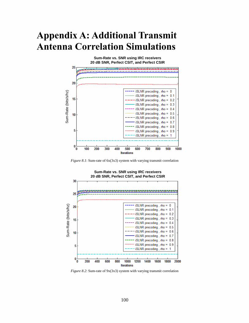
100

Appendix A: Additional Transmit

Antenna Correlation Simulations





Su

m-R

ate

(b

its/s

/hz)



Su

m-R

ate

(b

its/s

/hz)

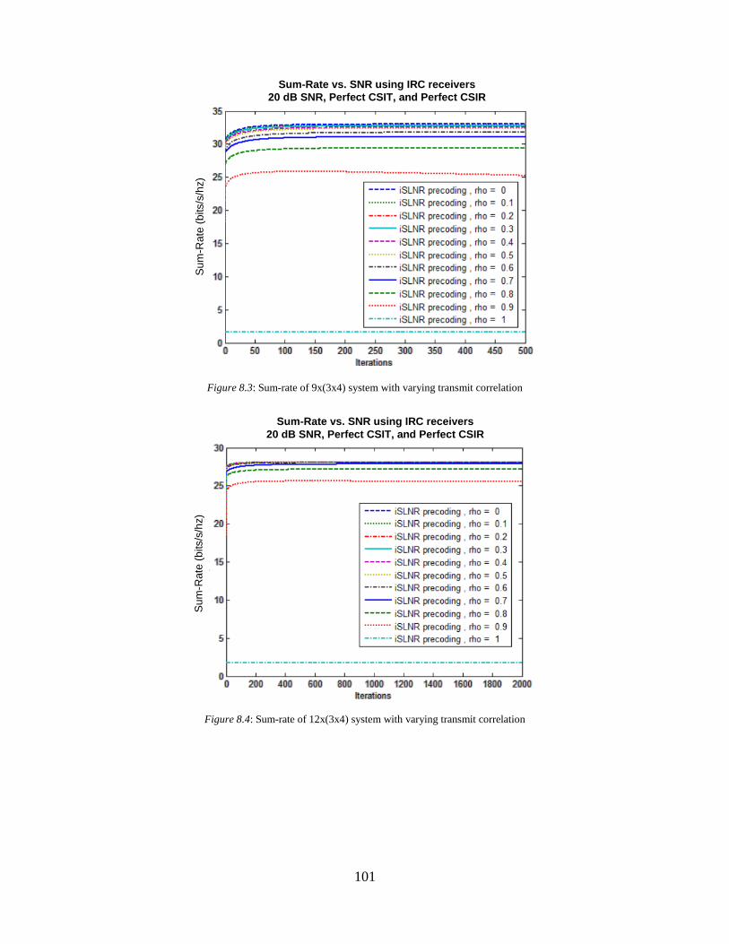
101





Su

m-R

ate

(b

its/s

/hz)



Su

m-R

ate

(b

its/s

/hz)

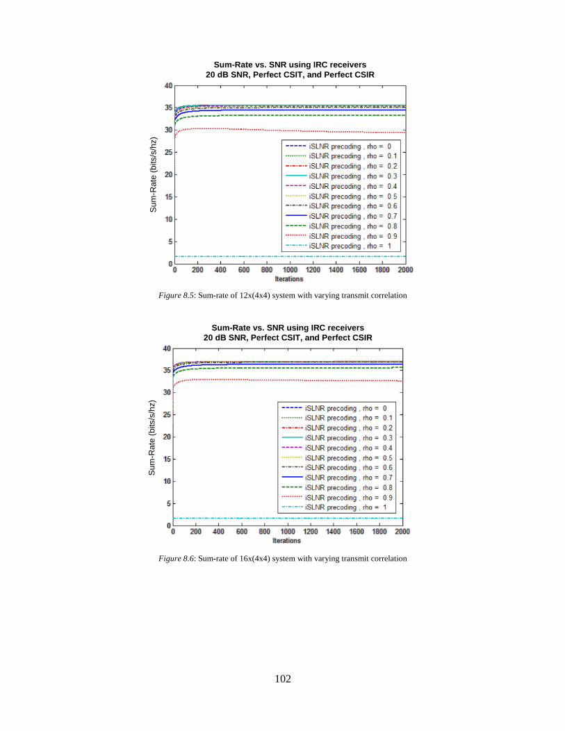
102





Su

m-R

ate

(b

its/s

/hz)



Su

m-R

ate

(b

its/s

/hz)

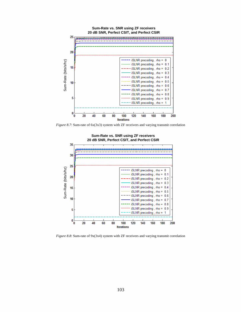
103

Figure 8.7: Sum-rate of 6x(3x3) system with ZF receivers and varying transmit correlation




Su

m-R

ate

(b

its/s

/hz)



Su

m-R

ate

(b

its/s

/hz)

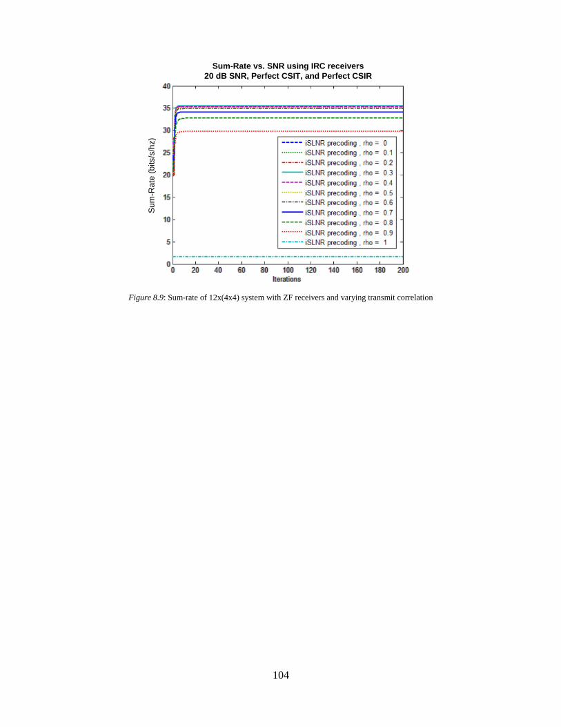
104




Su

m-R

ate

(b

its/s

/hz)

iterative leakage-based precoding for multiuser-mimo ... · convergence of the algorithm when using...

Documents