iterative learning control design for uncertain and time

Iterative Learning Control design foruncertain and time-windowed systems

proefschrift

ter verkrijging van de graad van doctoraan de Technische Universiteit Eindhoven,

op gezag van de Rector Magnificus, prof.dr.ir. C.J. van Duijn,voor een commissie aangewezen door het College voor Promoties

in het openbaar te verdedigenop woensdag 12 november 2008 om 16.00 uur

door

Jeroen Johan Maarten van de Wijdeven

geboren te Veghel

Dit proefschrift is goedgekeurd door de promotoren:

prof.ir. O.H. Bosgraenprof.dr.ir. M. Steinbuch

This dissertation has been completed in partial fulfillment of the requirements of theDutch Institute of Systems and Control, DISC, for graduate study.

A catalogue record is available from the Eindhoven University of Technology Library.

Iterative Learning Control design for uncertain and time-windowed systems / byJeroen J.M. van de Wijdeven. – Eindhoven : Technische Universiteit Eindhoven, 2008Proefschrift. – ISBN: 978-90-386-1435-9

Copyright c© 2008 by J.J.M. van de Wijdeven.

This thesis was prepared with the pdfLATEX documentation system.Cover Design: Oranje Vormgevers, Eindhoven, The NetherlandsReproduction: Universiteitsdrukkerij TU Eindhoven, Eindhoven, The Netherlands

iii

Contents

Nomenclature v

1 Introduction 11.1 Background . . . . . . . . . . . . . . . . . . . . . . . . . . . . . . . 11.2 Research objectives . . . . . . . . . . . . . . . . . . . . . . . . . . . 41.3 Outline of the thesis . . . . . . . . . . . . . . . . . . . . . . . . . . 9

2 Iterative Learning Control 112.1 A brief overview of ILC . . . . . . . . . . . . . . . . . . . . . . . . 122.2 Notations . . . . . . . . . . . . . . . . . . . . . . . . . . . . . . . . 152.3 ILC control objectives . . . . . . . . . . . . . . . . . . . . . . . . . 19

3 Time-windowed ILC 233.1 Point-to-point motion problem . . . . . . . . . . . . . . . . . . . . 243.2 ILC for residual vibration suppression: Hankel ILC . . . . . . . . . 273.3 Hankel ILC control design . . . . . . . . . . . . . . . . . . . . . . . 313.4 Example: two-inertia setup . . . . . . . . . . . . . . . . . . . . . . 343.5 Example: flexible beam setup . . . . . . . . . . . . . . . . . . . . . 393.6 Concluding remarks . . . . . . . . . . . . . . . . . . . . . . . . . . 46

4 ILC for systems with basis functions 494.1 Basis functions in ILC . . . . . . . . . . . . . . . . . . . . . . . . . 494.2 General ILC system description . . . . . . . . . . . . . . . . . . . . 544.3 ILC analysis for systems with basis functions, a system perspective 564.4 ILC analysis for systems with basis functions, a design perspective 584.5 Analysis of trial varying disturbances . . . . . . . . . . . . . . . . . 624.6 ILC controller design for systems with basis functions . . . . . . . 664.7 Reconsideration of basis function based ILC approaches in ILC

literature . . . . . . . . . . . . . . . . . . . . . . . . . . . . . . . . 684.8 Concluding remarks . . . . . . . . . . . . . . . . . . . . . . . . . . 69

5 ILC for uncertain systems: Robust convergence analysis 715.1 Uncertain system description . . . . . . . . . . . . . . . . . . . . . 725.2 Robust Monotonic Convergence objective . . . . . . . . . . . . . . 74

iv Contents

5.3 Robust Monotonic Convergence conditions . . . . . . . . . . . . . . 765.4 RMC conditions for structured ∆M . . . . . . . . . . . . . . . . . . 795.5 RMC for the uncertain systems with basis functions . . . . . . . . 835.6 Example: RMC of LQ norm optimal ILC control . . . . . . . . . . 855.7 Example: RMC simulations for LQ norm optimal ILC . . . . . . . 885.8 Concluding remarks . . . . . . . . . . . . . . . . . . . . . . . . . . 92

6 Noncausal finite time interval robust ILC control design 956.1 Noncausal finite time interval robust ILC control design . . . . . . 966.2 R-ILC analysis . . . . . . . . . . . . . . . . . . . . . . . . . . . . . 1006.3 R-ILC parameter optimization . . . . . . . . . . . . . . . . . . . . 1016.4 R-ILC design: State space solutions . . . . . . . . . . . . . . . . . 1046.5 R-ILC design for uncertain systems with basis functions . . . . . . 1126.6 Example . . . . . . . . . . . . . . . . . . . . . . . . . . . . . . . . . 1136.7 Concluding remarks . . . . . . . . . . . . . . . . . . . . . . . . . . 120

7 Conclusions and Recommendations 1237.1 Conclusions . . . . . . . . . . . . . . . . . . . . . . . . . . . . . . . 1237.2 Recommendations . . . . . . . . . . . . . . . . . . . . . . . . . . . 125

A Proofs and Derivations 127A.2 Chapter 2 . . . . . . . . . . . . . . . . . . . . . . . . . . . . . . . . 127A.3 Chapter 3 . . . . . . . . . . . . . . . . . . . . . . . . . . . . . . . . 128A.4 Chapter 4 . . . . . . . . . . . . . . . . . . . . . . . . . . . . . . . . 130A.5 Chapter 5 . . . . . . . . . . . . . . . . . . . . . . . . . . . . . . . . 132A.6 Chapter 6 . . . . . . . . . . . . . . . . . . . . . . . . . . . . . . . . 134

B Example: Allowable uncertainty for RC and RMC 141

C Flexible two-inertia setup 143

D Flexible beam setup 147

Bibliography 151

Summary 163

Samenvatting 165

Dankwoord 167

Curriculum Vitae 169

v

Nomenclature

Latin symbols[A Bi

Ci Dij

](i, j) ∈ [1, 2], state space matrices of a time domain system[

A BC D

]state space matrices of time domain system J[

Ah Bh

Ch

]elements of the time domain R-ILC controller

ATi, i ∈ [1, 2] system matrix of (partially) decoupled R-ILC controllerC time domain feedback controllerd scaling factordk(t) trial varying disturbance signaldγ tuning parameter for R-ILC controlD scaling matrixDM block diagonal scaling matrixDP scaling matrixDM the set of scaling matrices DM

e error signalf command signalfinit initial value for command signal fFTi, i ∈ [1, 2] system matrix of (partially) decoupled R-ILC controllerg learning gaing(t) state of the (partially) decoupled R-ILC controllerG generalized plant[Hij Fi

Gi Hy

](i, j) ∈ [1, 2], state space matrices of R-ILC controller

H general systemHc element of general system H with full row rankHo element of general system H with full column rankH∆ uncertain general system HIj j × j dimensional identity matrixj(t) impulse response of system J

vi Nomenclature

J systemJc element of system J with full row rankJH Hankel systemJo element of system J with full column rankJ∆ uncertain system JJ objective functionk trial index` trial periodicityL ILC control elementLc ILC control elementLim

c ILC control element Lc, including basis function matrix Tf

Lo ILC control elementm number of samples in 1) actuation time interval 2) basis func-

tions in Tf

m1 first sample of actuation time intervalm2 final sample of actuation time intervalM closed loop systemMc element of ILC control element Lc

n number of samples in 1) observation time interval 2) basisfunctions in Ty

n1 first sample of observation time intervaln2 final sample of observation time intervalN number of samples in a trialp rank of system matrix Jpk output signal of norm-bounded uncertainty ∆P plantPo element of ILC control element Lo

Pξ performance measure for variable ξk

Pξ,opt optimal performance measure for variable ξk

q number of inputs and outputs of uncertainty ∆qi number of system inputsqk input signal of norm-bounded uncertainty ∆qo number of system outputsQ weighting matrixQh matrix element of the time domain R-ILC controllerQ ILC control elementr weighting scalarR weighting matrixRh matrix element of the time domain R-ILC controllerRjj covariance matrix of signal js weighting scalarS weighting matrixSc element of ILC control element Lc

Sh matrix element of the time domain R-ILC controllerSo element of ILC control element Lo

Nomenclature vii

t time indexT similarity transformation matrixTc element of ILC control element Lc

Tf matrix with input basis functionsTs sample timeTy matrix with output basis functionsU left singular matrixu(t) controller output at time index tuk trial domain state vectorV right singular matrixVi system description of additive uncertainty in system H∆

Vo system description of additive uncertainty in system H∆

w(t) exogenous input signal at time index tW system description of additive uncertainty in system J∆

Wi system description of additive uncertainty in system J∆

Wo system description of additive uncertainty in system J∆

Wβ weighting matrixxk(t) time domain state vectorX variable in Sylvester equationyd reference signaly system output signalyref reference signalY Riccati variablez(t) performance objective at time index tzk trial domain state vector

Greek symbols

αd reference vector filtered by output basis function matrix Ty

αk output signal filtered by output basis function matrix Ty

βinit initial value for input signal of input basis function matrix Tf

βk input signal of input basis function matrix Tf

γ tuning parameter for R-ILC controlγmin approximate for γopt

γopt optimal value for the tuning parameter γ∆ norm-bounded uncertainty∆ the set of norm-bounded uncertainty ∆∆f maximum rate change of time domain command signal∆G norm-bounded uncertainty of generalized plant G∆M structured norm-bounded uncertainty of system M∆M the set of structured norm-bounded uncertainty ∆M

∆P unstructured norm-bounded uncertainty∆P the set of unstructured norm-bounded uncertainty ∆P

viii Nomenclature

εk error signal filtered by output basis function matrix Ty

ε infinitely small positive scalarζ(t) costate of fully decoupled R-ILC controllerθ frequency [rad/s]λ(t) costate of the R-ILC controllerξk performance variableΠ the set of uncertain systems J∆ over a finite time intervalΠz the set of z-domain uncertain systems J∆(z)Σ singular value matrixΨ the set of uncertain systems H∆ over a finite time interval

Subscripts, superscripts, and indices

a(t) signal a at time index ta(z) z-domain representation of signal aak vector a at trial kaas

k asymptotic value of a after convergence (trial varying)a0 initial condition of state a at trial k = 0a∞ asymptotic value of a after convergence (trial invariant)ai ith input of output signal of multi input multi output systemA(s) Laplace domain representation of system AA(z) z-domain representation of system AAij element (i, j) of matrix A

Special symbols and operations

aT transpose of vector aa time derivative of signal a|a| amplitude of scalar a‖a‖2 2-norm of vector aEa expected value of signal aAT transpose of matrix AA−1 inverse of matrix AA† Moore-Penrose inverse of matrix AA(1) 1-inverse of matrix A‖A‖i2 induced 2-norm of (system) matrix Aim(A) image space of matrix Aim(A)⊥ space perpendicular to the image space of matrix Aker(A) kernel space of matrix A

Nomenclature ix

rank(A) rank of matrix Aλ(A) eigenvalue of matrix Aρ(A) spectral radius of matrix Aσ(A) largest singular value of matrix AµB(A) structured singular value of matrix A with respect to B∂a∂b partial derivative of a with respect to bw one trial shift operator

R the set of real numbersRn the set of all n× 1 vectors with elements in RRn×m the set of all n×m matrices with elements in RC the set of complex numbersCn×m the set of all n×m matrices with elements in CL∞ the set of ∞-norm bounded signals∅ empty set∈ is an element of∀ for all7→ maps to≈ is approximately equal to:= is defined as6= is not equal to∑j

i summation from element i to j

Πji multiplication from element i to j

Acronyms and Abbreviations

det determinantdiag diagonalinf infimumlim limitmax maximummin minimum

2D 2-dimensionalCITE current iteration tracking errorDARE discrete algebraic Riccati equationDOF degrees of freedomHO higher orderi/o input/outputIMP internal model principleiff if and only ifILC Iterative Learning ControlLP linear programmingLQ linear quadratic

x Nomenclature

LTI linear time invariantLTV linear time varyingMC monotonic convergenceMIMO multi-input multi-outputP/PI/PD proportional/proportional plus intergral/proportional plus

derivativeR-ILC robust Iterative Learning ControlRC robust convergenceRMC robust monotonic convergenceSISO Single-input single-outputSVD singular value decomposition

1

Chapter 1

Introduction

In this chapter, we define our research objectives. For that, the ideabehind Iterative Learning Control (ILC) is introduced and its relationto other control techniques briefly discussed. Moreover, the use of time-windows in ILC is highlighted, and the consequences of model uncertaintyon ILC control design addressed.

1.1 Background

In numerous applications, a system has to perform a repeated batch task, e.g., apick and place machine or batch chemical process which has to follow a given refer-ence trajectory. Characteristic features of a batch task are that 1) each repetition(trial) spans a finite time interval which is known on beforehand, and 2) each trialstarts from the same initial conditions due to resetting of the system before eachtrial. Since the reference signal is, in general, the dominant disturbance in thesystem, this batch repetitiveness yields a servo error that is (approximately) equalfor each trial. If this servo error does not meet the performance specifications,Iterative Learning Control (ILC) can be introduced into the system to increaseperformance.

ILC iteratively improves the performance of repeated batch processes, by updatingthe feedforward signal (command signal) from one trial to the next using measureddata from previous trials, i.e., by learning from previous experience. The conceptbehind ILC is illustrated in Figure 1.1 and Figure 1.2. In Figure 1.1, a referencesignal and measured output are shown. In this example, ILC significantly reducesthe error between the reference signal and measured output within three trials.

2 Chapter 1: Introduction

0 0.5 1

0

0.5

1

trial 1po

sitio

n

0 0.5 1

0

0.5

1

trial 2

time0 0.5 1

0

0.5

1

trial 3

refmeas

Figure 1.1: Reference signal and measured output of the system for trials 1 to 3. Notethat in trial 3, the measured output and reference signal coincide.

0 0.5 1

−20

0

20

trial 1

For

ce

0 0.5 1

−20

0

20

trial 2

time0 0.5 1

−20

0

20

trial 3

Figure 1.2: Command signal generated by ILC for trials 1 to 3.

This is accomplished by iteratively updating the command signal, until the desiredcommand signal is obtained, see Figure 1.2.

The idea of using an iterative strategy to deal with repetitive disturbances is firstdescribed in a US patent from 1971, [53]. What seems to be the first academicpublication on ILC stems from 1978, [126]. But since it was in Japanese, the re-sults did not become widely spread. In 1984, [10, 25, 31] independently publishedresults on iterative improvement of performance. The term “Iterative LearningControl ” was introduced in Arimoto et al. in the same year, [11]. A first mono-graph on ILC stems from Moore 1993, [87]. Since then, treatment of differenttopics in ILC can be found in, e.g., [17, 22, 56]. Extensive surveys of different(industrial) applications of ILC is presented in [2, 88].

When properly designed, the ILC controller iteratively finds that command signalthat results in high performance, despite possible model uncertainty and unknown

1.1: Background 3

trial invariant disturbances. With the update of the command signal based onpreviously measured data, the trial-to-trial behavior of ILC can be considered afeedback process. On the other hand, during the time interval of a trial, thiscommand signal is applied to the system as a fixed feedforward signal. Conse-quently, it depends on the domain, trial domain or time domain, whether ILCcan be considered as feedback or feedforward control.

Based on the feedforward characteristics of ILC in time domain, its iterativesearch for the optimal command signal in trial domain, and the fact that ILC isdesigned to compensate for (trial) repetitive disturbances, we briefly discuss sim-ilarities and differences between ILC for linear systems and ILC related controlstrategies.

Model-based feedforward controlThe basic idea of feedforward control is to find a feedforward signal f such thatthe system’s output y follows the reference signal yref , i.e., y = Pf with f suchthat yref − y = 0. Under the assumption that a model P of the system dynamicsis known and P−1 is stable, inverse model feedforward control can be applied toobtain the optimal feedforward signal: f = P−1yref , see e.g., [18]. Note thatcausality of the inverse is of no importance, since the input of the feedforwardcontroller (the reference signal) is assumed known for all time, both past andfuture.

A benefit of model-based feedforward over ILC is that a feedforward signal canbe obtained for arbitrary reference signals without the need for iterative learning.A drawback of these controllers is, however, that the amount of performance im-provement strongly depends on the accuracy of the model, see e.g., [36].

Adaptive feedforward controlIf the system structure is known but its parameters are uncertain, then the feed-forward signal can be obtained using an adaptive feedforward controller, i.e., afeedforward controller which recursively estimates system (related) parameters,see e.g., [9, 74]. To obtain the optimal command signal such that yref − y = 0,we require the inverse of the true system structure to be contained in the modelstructure of the controller. However, even if the inverse system structure is notcontained in the controller, this approach will result in optimized performance inthe space in which parameter estimation can occur. Estimation of the parameterscan subsequently be performed on-line in time domain, leading to the condition ofpersistency of excitation of the reference signal, or off-line in trial domain, betweentwo trials. In this thesis, we consider trial domain adaptive feedforward controlin a restricted input/output (i/o) space to be a specific case of ILC, see Chapter 4.


Repetitive controlILC is comparable to repetitive control, [35, 63, 118, 124], in the sense that theyboth strive after performance improvement by reducing the effects of periodicdisturbances on the error. An essential difference between repetitive control andILC, however, is that an ILC controlled system is reset between two trials, whilea system controlled with a repetitive controller is not. A first consequence is, thatILC can handle batch repetitive disturbances in time domain, e.g., a referencedisturbance which is equal from trial to trial, and repetitive control can handledisturbances which are repetitive (periodic) in time domain, e.g., a continuouslyrotating disc with a disturbance that occurs each revolution. A second conse-quence is, that repetitive control can be considered a feedback control strategy intime domain, instead of a feedforward control strategy in time domain.

1.2 Research objectives

In this section, we formulate the research objectives which form the basis forthis thesis. These objectives can be divided into two subjects: The first subjectaddresses the use of time windows in ILC. The second subject raises the issue ofrobustness of ILC against model uncertainty.

1.2.1 Motivation

Our interest for ILC for time-windowed systems is founded in industrial applica-tions. One application in which time-windowed ILC is used (implicitly), is thesemiconductor industry. In [85], for example, the ILC control problem is modifiedsuch that performance is only improved during the time intervals in a trial wherethe repetitive disturbances dominate the non-repetitive disturbances. In [13], abatch iterative approach is used to improve the performance during the scanningtime interval of a trial. Another application is given by the Ultra High Pressure(UHP) lamp for projection systems, [122]. Due to computation and memory de-mands, in [122] the lamp is actuated over a time interval which is shorter thanthe time interval in which the lamp’s output is measured. Although the imple-mentations have been shown to be successful, the implications of time-windowedsystems on ILC control design are not yet known.

In ILC literature, many successful implementations of ILC have been presented.These results are, however, most often based on the implementation of ILC on asingle sample system (of a mass produced system). Furthermore, the experimentsare often conducted over a limited time span, e.g., days, weeks. What will happen,if a designed ILC controller is applied to a different sample system, or to a systemwhose dynamics have changed due to wear? To our opinion, ILC literature doesnot provide fully satisfying answers to these for industry essential questions.

1.2: Research objectives 5

1.2.2 ILC for time-windowed systems

Before any proper ILC design can take place, it has to be apparent which taskILC is expected to carry out, i.e., the ILC problem formulation has to be clear.As we discuss below, in many situations a correct formulation of the problemrequires the use of time windows. These windows can be used to select specifictime samples at the input and output of the system, as illustrated in Figure 1.3.

t i m e

output

output

output

output

t i m e

t i m e t i m e

Figure 1.3: Top: A time window is used to select a specific time interval of the timesignal. Bottom: Downsampling of the time signal.

One of the most well known problem formulations in ILC deals with the servotask. In this task, ILC control has to iteratively generate a command signalwhich actuates the system during the complete time span of a trial, such that theobserved output of the system follows a certain predefined reference trajectoryduring the complete time span of a trial.

In another ILC task, one is only interested in the output of the system at theend of the trial, see e.g., [29, 54, 137]. Actuation in this so-called terminal ILCtakes place during the complete time span of the trial, while observation of theerror occurs only at the final time sample of the trial. An example of terminalILC is rapid thermal processing, [137]. The goal is to control the chemical vapordeposition thickness on a wafer at the end of the process by controlling the wafertemperature. Any thickness errors during the process are of no interest.

A third ILC task is found in residual vibration suppression in point-to-point mo-tion problems, see [40, 78, 79, 133]. This problem formulation covers the case inwhich residual vibrations are to be suppressed, after the system has been movedfrom an initial position to a desired position. This requires actuation of the sys-tem during the motion from initial to final position, and observation of residualvibrations after arrival at the desired point.


The previous three ILC problem formulations resulted in the definition of specifictime intervals in which actuation and observation of the system is allowed. Otheruses for time windows are, however, also possible, e.g., to study the time domainand trial domain behavior of the servo error signal. In [7, 66, 76], performanceand convergence properties of systems with nonzero relative degrees and delaysare studied. To properly analyze the convergence properties of the system understudy, [7, 66, 76] implicitly make use of time windows. Namely, the actuationinterval of the system is reduced by removal of the final samples of the trial inter-val, and the observation time interval is reduced by removal of the first samplesof the trial interval. In [68, 142], the error convergence from trial to trial has tosatisfy specific monotonicity conditions. By downsampling of the original system,these conditions are met. Downsampling for reduction of inter-sample behaviorin ILC is discussed in [77]. In [72], reduction of inter-sample behavior is achievedby removing the first number of actuation samples in a trial. Finally, in [98, 99],inter-sample behavior in ILC is studied using a multirate system representationwhich is constructed with time windows.

From the previous discussion, we conclude that time windows in ILC are widely,though often implicitly, used to properly formulate ILC problems. This observa-tion leads to the first research objective:

Objective 1. Explore the design issues, i.e., problem formulation, con-vergence analysis, and ILC control design, in ILC for time-windowed sys-tems.

Time-windowed systems can be considered a specific subset of systems with i/obasis functions. This observation leads to the second research objective:

Objective 2. Formulate a unifying ILC design framework which encom-passes the different ILC problem formulations for linear systems withbasis functions, and determine the for ILC relevant properties of thisframework.

In Section 2.1, we elaborate on different ILC control suggestions and formulationsin ILC literature, and discuss which ones we will consider in this thesis. Inobjective 2, we aim at formulating a unifying framework which is valid for theseconsidered systems and ILC control suggestions.

1.2: Research objectives 7

1.2.3 ILC for uncertain systems

Although the command signal generated by the ILC control strategies is basedon measured data, most often the ILC controller is designed using a model of thesystem. The majority of the ILC control strategies discussed in ILC literaturecan be divided into three categories, [96].

Arimoto gainsArimoto gains (or P/PD/PI-type), [26, 48, 76, 140], are ILC controllers in whichthe command signal is updated with a scaled, positive time shifted error signal.These controllers have as great benefit that they can iteratively find optimal com-mand signal using very little information about the system. This, however, goes atthe expense of the ease with which specific convergence properties can be achieved.

Inverse model based ILCIn inverse model based ILC, [12, 83, 106, 119, 132, 139], the ILC controller isbased on the inverse of a model of the system. With an accurate model, conver-gence of the ILC algorithm occurs in just a few iterations. On the other hand,with a poor model, the ILC algorithm can result in unstable behavior.

Linear quadratic (LQ) norm optimal ILCFinally, LQ norm optimal ILC, [7, 38, 58, 107], focusses on ILC control designwhich results from a quadratic optimization problem. Depending on the formu-lated objective, different parameters in the ILC controller can be used to influencedifferent properties of the ILC algorithm. In its most simple form, LQ norm op-timal ILC equals inverse model based ILC. Although this control strategy doesrequire a model of the system, and tuning of the controller can be more exten-sive than the other two control strategies, it can be designed to be less sensitiveagainst model uncertainty than inverse model based ILC.

Since no model can truly reflect the real system behavior, the controller is requiredto have some robustness against model uncertainty. Depending on the amountof uncertainty present and on the properties of the controller itself, the ILC con-trolled system can become unstable in trial direction, rendering ILC useless.

Robustness analysis of ILC controllersIt is known that, to a certain extent, each ILC controller incorporates robustnessagainst model uncertainty. In [64], it is shown that there exists inverse modelbased ILC controllers for which the ILC controlled system is robustly mono-tonically convergent, provided that the multiplicative uncertainty description ispositive real. In [6, 52, 55, 56, 70], the robustness properties of LQ norm optimalILC controllers are discussed. Although in [6, 52], the finite time interval aspect


of ILC is explicitly included in the robust convergence analysis, the approach doesnot leave room to include uncertainty models. As a result, the robustness proper-ties of the solution can not be quantified. In contrast, in [55], uncertainty modelscan be included in the analysis. With the analysis based on a frequency domainrepresentation of the ILC controller, however, the results are only approximatewhen applied to a finite time interval. Namely, the Fourier transform on the infi-nite time interval which is used in this approach, leads to a linear time invariant(LTI) control law. The application of this LTI controller on a finite time intervalof a trial may result in errors in the initial part of the transient behavior. In [56],the finite time interval presentation of the system and controllers is approximatedin a Fourier basis, leading to a not fully clear definition of the uncertainty modeland a number of approximate robustness results. Robustness of LQ norm optimalILC over a finite time interval for multiplicative model uncertainty representedby a gain is studied in [70]. Finally, in [4], a robust convergence analysis approachis presented which is applicable to any linear trial invariant ILC controller. How-ever, the specific problem formulation used in [4] may restrict the utility of theresults.

Robustness by design of robust ILC controllersNext to analysis of given ILC controllers with respect to robustness, robustnesscan be enforced by design of robust ILC controllers. Robust ILC controllers in-corporate an uncertainty model in the design of a controller, so as to improverobustness and performance of the ILC controlled system. Most of these controlstrategies pose the ILC control design problem as an H∞ optimization problem.In [51, 114], the robust control problem is represented by a 2D system represen-tation. Subsequently, a combined state feedback controller in time domain andArimoto gain ILC controller in trial domain is designed. Hence, full knowledgeof the time domain system states is required. In [8, 34, 41, 120, 135], the designproblem is posed in frequency domain, and therefore only approximates the truefinite time interval problem. Moreover, the resulting H∞ optimal controllers arecausal, i.e., the command signal in trial k + 1 at time index t∗ only depends oninformation of trial k at time indices t ∈ [0, 1, . . . , t∗] (see Section 2.2 for a formalintroduction of the terms “causal” and “noncausal” in ILC). It is shown, see e.g.,[97], that specific (often desirable) convergence properties of the ILC controlledsystem can be achieved with noncausal ILC controllers only. In [89], the robustILC control problem is formulated as an H∞ problem in the trial domain, withmodel uncertainty which is assumed to be trial varying, i.e., model uncertaintywhich can change from one trial to the next.

To solve a constrained robust ILC control problem for systems under worst casetrial varying uncertainty, in [70], a min-max optimization problem is formulated.Due to the problem formulation, no analytical solution for the ILC controllercan be given. Moreover, the solution is computationally demanding. Finally,robust ILC control design for systems with interval uncertainty is studied in [1].The uncertainty model used puts an individual error bound on each element ofthe impulse response, which leads to a large computational load for a realisticproblem.

1.3: Outline of the thesis 9

Summarizing this discussion, the following aspects should ideally be covered inILC control design approaches for uncertain systems:

• the finite time interval aspect of a trial (for an accurate representation ofthe ILC problem),

• the freedom to include uncertainty models in the design process (to improveachievable performance, and to be able to quantify robustness properties),

• and the possibility to analyze the robustness properties of various ILC con-trol strategies (generality of the analysis).

The current approaches in literature all neglect one or more of these aspects. Thisobservation leads to the following final two objectives:

Objective 3. Develop a robust convergence analysis approach whichcovers the finite time interval aspect of ILC, is applicable to linear trialinvariant ILC strategies, and can incorporate uncertainty models in itsanalysis.

Objective 4. Develop a robust ILC control strategy which exploitsknowledge about model uncertainty in its design, is not restricted to becausal, and incorporates the finite time interval aspect of ILC.

1.3 Outline of the thesis

This thesis is organized as follows. In Chapter 2, we introduce the ILC repre-sentation used throughout this thesis. Based on this representation, the systemnotations and ILC control structure are introduced, together with preliminaryresults on ILC control objectives such as convergence and performance.

Chapters 3 to 6 follow the order of the objectives as given in Section 1.2. Asa result, in Chapter 3, we focus on Objective 1. With ILC for residual vibra-tion suppression in point-to-point motion systems largely unexplored, we use thisILC task as an exemplary case to analyze ILC for time-windowed systems. Thisanalysis not only leads to a better understanding of ILC for point-to-point mo-tion problems, it also reveals new design freedom in ILC. We illustrate this newfreedom by presenting experimental results on flexible systems.


In Chapter 4, we formalize and extend the results of Chapter 3 to systems withbasis functions by formulating an ILC framework which encompasses the dis-cussed time-windowed systems as a special case. An ILC analysis and designtheory for systems with basis functions reveals how multiple ILC control objec-tives can be reached without the need to compromise between them, includingthe compensation for the effects of trial varying disturbances on performance.

In Chapter 5, we derive a robust convergence analysis approach for ILC controlledsystems. The proposed approach is based on well developed µ analysis [103, 117,143], in a form which respects the finite time interval aspect of ILC. Moreover, theanalysis can handle additive and multiplicative uncertainty models in its problemformulation, and can be applied to MIMO linear time invariant systems controlledwith any possibly noncausal linear trial invariant ILC controller. To exemplifythe results, we analyze the robust convergence properties of LQ norm optimalILC.

In Chapter 6, we develop a robust ILC control strategy which incorporates an ad-ditive uncertainty representation in its design. For the derivation of the controller,we use an approach similar to H∞ optimization, however, formulated such thatthe solution is not restricted to be causal and explicitly acts on a finite time inter-val. By means of experiments, we show that the proposed R-ILC controller canoutperform LQ norm optimal ILC and robust ILC based on a frequency domainµ procedure.

Finally, conclusions and recommendations are presented in Chapter 7.

11

Chapter 2

Iterative Learning Control

In this chapter, we discuss different formulations in ILC and extract theILC representation which we will use throughout this thesis. Based onthis representation, the system notations and ILC control structure arepresented. Moreover, ILC control objectives are introduced and prelimi-nary results with respect to these objectives are given.

Introduction

The general idea of ILC is illustrated in Figure 2.1, [87]. In Figure 2.1, J representsthe system under study, ILC is the ILC algorithm, and the subscript k denotesthe trial index with k = 0, 1, 2, . . .. The idea behind ILC is as follows. During trialk, a command signal fk is applied to system J . This command signal is storedin a memory, together with the error ek which equals the difference between thereference signal yd and system output yk. After the trial has ended, the commandand error signal are fed to the ILC algorithm, resulting in a command signal fortrial k + 1, i.e., fk+1 = ILC(fk, ek). Ideally, the ILC controller will iterativelygenerate a command signal, from trial to trial, such that the error ek convergesto zero.

Throughout this thesis, we assume the following to hold, [17, chap. 1].

1. Every trial has a fixed finite time span.

2. The system under study is reset to the same initial conditions at the be-ginning of each trial, i.e., xk(0) = x0 for k = 0, 1, 2, . . .. Without loss ofgenerality, we can take x0 = 0.

12 Chapter 2: Iterative Learning Control

fk+1

ekfk

yd

yk

ILCJ

+−

Figure 2.1: General ILC framework.

3. The system dynamics are trial invariant.

4. The output signal used for ILC is available from measurements.

2.1 A brief overview of ILC

From the ILC literature, multiple suggestions for the formulation of the ILC prob-lem are available. In this section, we briefly discuss some of the more well knownsuggestions and discuss which we will use in this thesis. For a more elaborateoverview of the different issues in ILC, see e.g., [2, 88].

2.1.1 Problem description

The ILC problem is a 2-dimensional (2D) control problem, i.e., information prop-agation occurs in two independent directions, e.g., [87]. On the one hand, we havethe finite time domain behavior of the system during a trial. On the other hand,we have the trial behavior from trial to trial. To capture the 2D system behavior,different problem descriptions are possible.

It is possible to formulate the ILC problem as 2D control problem, e.g., usinga Roesser or Fornasini-Marchesini state-space model, [51, 73, 102, 114]. Withinthis formulation, the finite time domain behavior and discrete trial domain behav-ior are easily captured. Furthermore, control design can incorporate both timeand trial domain objectives. ILC analysis and control design is, however, moreinvolved.

To simplify ILC analysis and design, the ILC problem can be approximated byconsidering the time domain to be infinite in length. As a result, the time domainbehavior of systems can be represented by transfer functions and analysis can bedone in frequency domain, e.g., [8, 23, 139]. The use of the frequency domainrepresentation over a finite time interval does, however, lead to approximationerrors (see Chapters 5 and 6).

Finally, the ILC problem can be described using a lifted notation, see e.g., [12,60, 86, 100, 105, 119]. The idea behind the lifted notation is, that the finite time

2.1: A brief overview of ILC 13

domain behavior of a system is enclosed in a 1D notation in trial domain. Asa result, ILC analysis can be executed using standard linear control theory, andtime domain behavior is defined in a finite time interval. In contrast to 2D ILC,where stability can be considered in both time and trial domain, stability analysisin lifted ILC is restricted to trial domain convergence. Furthermore, “lifting” ofthe time domain behavior can result in large system representations, e.g., systemmatrices J of dimensions of 1000×1000 (which in ILC literature is sometimesabusively referred to as “curse-of-dimensionality”).

Due to the simplicity of the ILC problem description, available analysis theoryfrom linear control theory and linear algebra, the explicit inclusion of the finitetime aspect in its description, and the ease with which basis functions can beincluded in this representation, in this thesis, we use the lifted ILC notation todescribe our ILC problems.

2.1.2 (Non)linear systems

In many applications, the system behaves nonlinearly. In general, ILC controldesign for nonlinear systems is more complex than that for linear systems, seee.g., [28, 136]. One approach to obtain a linear system behavior of a nonlinearsystem, is to linearize the system using feedback linearization, e.g., [83]. Thisresults in a linear time invariant (LTI) system description. Another approach isto apply time domain feedback control to the nonlinear system to get the system’soutput in the vicinity of desired trajectory. Subsequently, the feedback controlledsystem can be linearized around the trajectory to give a linear time varying (LTV)system representation, e.g., [107].

In this thesis, we limit ourselves to applications which can be described by, orwell enough approximated by, LTI or LTV models. These models can be properlycaptured by the lifted system representation.

2.1.3 Continuous versus discrete time

In ILC, information propagation occurs in two independent directions: the timeand trial direction. While the behavior in trial domain is discrete, the behaviorof the physical time domain system is most often continuous. This can be takeninto account in ILC control design by describing the time domain behavior by acontinuous time model, see e.g., [10, 17, 104, 136]. Implementation of the ILCcontroller, however, must be digital, due to storage of the command and errorsignal in a digital memory. Using the reasoning: “With the implementation ofILC control digital, the design of the controller might as well acknowledge thisfrom the start”, [17, chap. 7], in this thesis we represent the time domain systembehavior in discrete domain.


2.1.4 First order, higher order, and current iteration trackingerror ILC

The basic idea behind ILC is to use the command signal f and error signal e fromtrial k to determine the command signal for trial k + 1, i.e., fk+1 = ILC(fk, ek).In case calculation of fk+1 is based on these signals only, the ILC controller isreferred to as first order ILC.

If signals from earlier trials are also included in the ILC algorithm, i.e., if fk+1 =ILC(fk, fk−1, . . . , ek, ek−1, . . .), the algorithm is referred to as higher order (HO)ILC, [5, 17]. Depending on the proposed ILC control strategy, performance of HOILC in presence of trial varying disturbances can be increased, [59], or not [91,111]. Similarly, depending on the used ILC control strategy, robustness and/orconvergence properties can be improved, [66, 89], or not, [91].

Next to inclusion of multiple past trial signals, it is also possible to use currentiteration error signals in the ILC algorithm, i.e., fk+1 = ILC(fk, ek, ek+1). ThisILC controller is referred to as current iteration tracking error (CITE) ILC, [27,30, 97]. A closer look at the structure of CITE ILC reveals that this ILC algorithmcombines first order ILC with time domain feedback control. As a result, CITEILC can improve performance of the ILC controlled system in presence of trialvarying disturbances and improve robustness, similar to time domain feedbackcontrol.

In this thesis, the emphasis is on trial invariant phenomena. Furthermore, weassume that the system under study is already stable, or stabilized by a timedomain feedback controller. Consequently, we consider first order ILC only.

2.1.5 Trial (in)variance

Up to now, the discussed ILC strategies have been trial invariant, i.e., the ILCcontrollers do not vary from one trial to the next. In presence of trial varyingphenomena, the ILC control algorithms can be made trial varying, i.e., fk+1 =ILCk(fk, ek), e.g., [49, 50, 65, 67, 84, 92]. Using the argument that the emphasisin this thesis is on trial invariant phenomena, we restrict ourselves to trial invariantILC.

2.1.6 Model uncertainty

Since no model can fully capture the dynamic behavior of the real system, modeluncertainty will always be present. This uncertainty can be ignored in ILC controldesign, i.e., ILC control design is based on the assumption that the model andsystem behavior coincide. Conversely, model uncertainty can be explicitly takeninto account in ILC control design, see e.g., [1, 34, 56, 92, 121].

2.2: Notations 15

In this thesis, we dedicate a significant part to ILC for uncertain systems (seeChapter 5 and Chapter 6).

2.1.7 Disturbance aspects

Finally, we address the issue of disturbances in ILC, [7]. Next to the trial in-variant reference signal yd, external trial varying disturbances, e.g., originatingfrom measurement noise, neighboring systems, etc., can be present in the ILCproblem, see [30, 70, 94, 111, 112, 123]. Another source of disturbances originatesfrom errors in the resetting of the system at the beginning of a trial, denoted asinitial condition disturbances, [27, 46, 82, 101].

We briefly discuss performance in presence of trial varying disturbances (see Sec-tion 4.5). In contrast, as discussed in the introduction of this chapter, we assumethat the initial conditions remain unchanged from one trial to the next. In otherwords, we do not consider initial condition disturbances.

2.2 Notations

Based on the choices made in Section 2.1, in this section, we introduce the sys-tem representation and a commonly used ILC control framework. The controlobjectives related to this framework are defined in Section 2.3.

2.2.1 Lifted system representation

Consider the LTV system J as given in (2.1), with f(Tst) ∈ Rqi the commandsignal, and y(Tst) ∈ Rqo the output signal.

J :

x(Ts(t + 1)) = A(Tst)x(Tst) + B(Tst)f(Tst)y(Tst) = C(Tst)x(Tst) + D(Tst)f(Tst).

(2.1)

Time index t denotes the sample number, and Ts represents the sample time. Notethat in ILC, the time span of a trial is finite, and hence that Tst ∈ [0, Ts(N − 1)]with N ∈ N the number of samples in a trial. The sample time Ts is omitted forbrevity.

In time domain, system J represents an open or closed loop system, see Figure 2.2(possibly with C = 0). Input yref (t) ∈ Rqo in Figure 2.2 denotes the referencesignal, f(t) ∈ Rqi the command signal generated by the ILC algorithm, finit(t) auser defined initial feedforward signal (possibly zero), and e(t) ∈ Rqo the measurederror signal.


f(t) finit(t)

yref (t)

e(t)

C P

J

+++ ++

−

Figure 2.2: General time domain closed loop system.

The i/o mapping (yref (t), f(t), finit(t)) 7→ e(t) is given by

e(t) = (Iqo+ PC)−1yref (t)− (Iqo

+ PC)−1P (f(t) + finit(t)).

To fit this mapping to the ILC framework of Figure 2.1, we define yd(t) ∈ Rqo

and J : f(t) 7→ −e(t) by

yd(t) := (Iqo + PC)−1(yref (t)− Pfinit(t))

J := (Iqo+ PC)−1P,

resulting in

e(t) = yd(t)− Jf(t). (2.2)

An initial command signal finit(t) is hence enclosed in the definition of signalyd(t). For finit(t) = 0 and C = 0, clearly yd(t) = yref (t). For finit(t) 6= 0and/or C 6= 0, signal yd(t) represents the servo error signal in absence of ILC.Nevertheless, independent of the specific choice for C, the goal of ILC is to finda command signal f(t) such that e(t) = 0.

Using the definitions of yd and J , Figure 2.2 is equivalent to Figure 2.3. In theremainder of this thesis, we refer to yd(t) as the reference signal and J as thesystem (under study).

e(t)f(t)

yd(t)

y(t)J

+−

Figure 2.3: General time domain closed loop system with definitions yd and J .

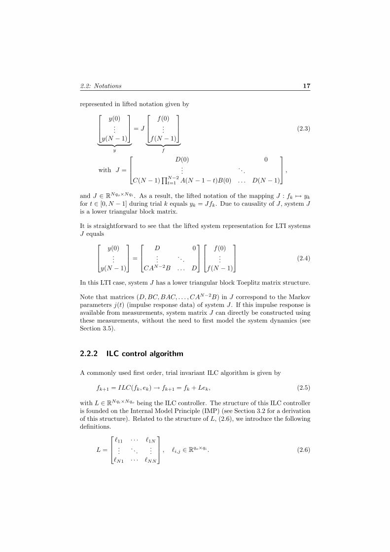
For the time span of a trial t = 0, 1, . . . , N − 1, the i/o behavior of J can be

2.2: Notations 17

represented in lifted notation given by y(0)...

y(N − 1)

︸︷︷︸

y

= J

f(0)...

f(N − 1)

︸︷︷︸

f

(2.3)

with J =

D(0) 0...

. . .C(N − 1)

∏N−2t=1 A(N − 1− t)B(0) . . . D(N − 1)

,

and J ∈ RNqo×Nqi . As a result, the lifted notation of the mapping J : fk 7→ yk

for t ∈ [0, N − 1] during trial k equals yk = Jfk. Due to causality of J , system Jis a lower triangular block matrix.

It is straightforward to see that the lifted system representation for LTI systemsJ equals y(0)

...y(N − 1)

=

D 0...

. . .CAN−2B . . . D

f(0)

...f(N − 1)

(2.4)

In this LTI case, system J has a lower triangular block Toeplitz matrix structure.

Note that matrices (D,BC, BAC, . . . , CAN−2B) in J correspond to the Markovparameters j(t) (impulse response data) of system J . If this impulse response isavailable from measurements, system matrix J can directly be constructed usingthese measurements, without the need to first model the system dynamics (seeSection 3.5).

2.2.2 ILC control algorithm

A commonly used first order, trial invariant ILC algorithm is given by

fk+1 = ILC(fk, ek) → fk+1 = fk + Lek, (2.5)

with L ∈ RNqi×Nqo being the ILC controller. The structure of this ILC controlleris founded on the Internal Model Principle (IMP) (see Section 3.2 for a derivationof this structure). Related to the structure of L, (2.6), we introduce the followingdefinitions.

L =

`11 · · · `1N

.... . .

...`N1 · · · `NN

, `i,j ∈ Rqo×qi . (2.6)


Definition 2.1 (Causal ILC control). Given ILC controller L, (2.6). Then L iscalled causal if ìj = 0 for j > i.

For L causal, the command signal fk+1(t∗) is a function of ek(t) with t ∈ [0, t∗],i.e., the update of the command signal fk+1 − fk at time t∗ ∈ [0, N − 1] dependsonly on error samples ek in the past (time interval 0 ≤ t ≤ t∗).

Definition 2.2 (Noncausal ILC control). Given ILC controller L, (2.6). Then Lis called noncausal if ìj 6= 0 for (some) j > i.

For L noncausal, the command signal fk+1(t∗) is a function of ek(t) with t ∈[0, N −1], i.e., the update of the command signal fk+1−fk at time t∗ ∈ [0, N −1]depends on error samples in the future (t∗ < t ≤ N − 1).

Definition 2.3 (Linear time invariant ILC control). Given ILC controller L,(2.6). Then ILC controller L is called LTI if ì,j = ì,i−k for k ∈ [−N + 1, N − 1],i.e, if L has a block Toeplitz structure.

Definition 2.4 (Linear time varying ILC control). Given ILC controller L, (2.6).Then ILC controller L is called LTV if it is not LTI, i.e, if L does not have a blockToeplitz structure.

2.2.3 ILC controlled system

By combining the lifted representation of (2.2) with (2.5), we find the ILC frame-work presented in Figure 2.4, with w corresponding to the one trial shift operator:fk+1 = wfk. We refer to the feedback system in Figure 2.4 as the ILC controlledsystem. Throughout this thesis, the dimensions of the system blocks in the dia-grams represent the dimensions of the corresponding system matrices.

fk+1 ekfk

yd

ykw−1I J

L

+ +

+

−

Figure 2.4: First order, trial invariant ILC framework.

With the ILC controlled system a feedback system in trial domain, we can expressits trial domain open loop dynamics by

fk+1 = fk + Lek, f0 = 0 (2.7)yk = Jfk, ek = yd − yk,

2.3: ILC control objectives 19

and trial domain closed loop dynamics by

fk+1 = (I − LJ)fk + Lyd, (2.8)

with f0 = 0. Recall that any nonzero initial command signal finit is enclosedin the definition of yd, and hence that we can consider f0 = 0 without loss ofgenerality.

In Section 2.3, we use these dynamics to study properties of the ILC controlledsystem.

2.3 ILC control objectives

The ILC control objectives that we discuss in this section are shown in Figure 2.5.In the discussions, we make use of the following definitions: The 2-norm of a vectorp is given by ‖p‖2 =

√pT p ≥ 0. The induced 2-norm of a finite dimensional

system matrix P is given by ‖P‖i2 = σ(P ), with σ(P ) the largest singular valueof P .

N o r m - o p t i m a l i t y

M o n o t o n i c c o n v e r g e n c e

C o n t r o l o b j e c t i v e sC o n v e r g e n c e

P e r f o r m a n c e

C o n v e r g e n c e s p e e d

Figure 2.5: ILC control objectives.

2.3.1 Convergence

Convergence of the ILC controlled system in trial domain is essential, see e.g.,[95, 109]. With (2.8) describing the evolution of the system in trial domain andfk representing the state in trial domain, convergence of the ILC controlled systemcan be defined as follows.

Definition 2.5 (Convergence). Given ILC controlled system (2.8) with yd = 0and f0 ∈ RNqi . Then (2.8) is convergent iff f∞ = 0 ∀f0 ∈ RNqi , with f∞ =limk→∞ fk.

Note that convergence can also be defined as function of the output yk or theerror ek. We, however, choose to focus on convergence of the command signal fk.


A standard result in stability theory now states that convergence is achieved ifand only if the coefficient matrix of (2.8) has spectral radius smaller than one,i.e. ρ(INqi

− LJ) < 1 with ρ(·) = maxi |λi(·)| and |λi| the absolute value of theith eigenvalue.

Convergence states that for any initial state f0, the command signal fk will be zeroafter an infinite number of trials. It does, however, not provide any informationabout transient behavior of fk between k = 0 and k →∞. In Definition 2.6, thistrial domain transient behavior of fk is taken into account.

Definition 2.6 (Monotonic Convergence (MC)). Given ILC controlled system(2.8) with yd = 0 and f0 ∈ RNqi . Then (2.8) is monotonically convergent (MC)in the variable fk if there exists 0 ≤ κ < 1 such that

‖fk+1‖2 ≤ κ‖fk‖2, ∀f0 ∈ RNqi , (2.9)

and ‖fk+1‖2 = ‖fk‖2 only for fk = fk+1 = 0.

Based on Definition 2.6, the following sufficient MC condition can be formulated.

Lemma 2.1. Given ILC controlled system (2.8). Then (2.8) is MC in fk if‖INqi − LJ‖i2 < 1.

Proof. See Appendix A.2.1.

Lemma 2.1 states that a sufficient condition for monotonic convergence of (2.8)in fk is given by ‖INqi

− LJ‖i2 < 1. Or, in other words, monotonic conver-gence requires that the largest gain in INqi

− LJ is smaller than one, i.e., thatσ(INqi−LJ) < 1. Consequently, demands on monotonic convergence of (2.8) canbe represented by demands on the gain σ(INqi − LJ).

Remark 2.1. With ρ(·) ≤ ‖ · ‖i2, monotonic convergence of the ILC controlledsystem in fk implies convergence of the ILC controlled system.

Remark 2.2. We derived the MC condition based on Definition 2.6. Alternatively,the same MC condition can be found by considering yd 6= 0 and f0 = 0. The onlydifference between the two approaches is found in the definition of MC. For yd 6= 0and f0 = 0, monotonic convergence requires ‖fk+1 − f∞‖2 < κ‖fk − f∞‖2.

Remark 2.3. In general, monotonic convergence of the command signal fk doesnot imply monotonic convergence of the output signal ek, [3, 22]. In certaincases, however, monotonic convergence of the command signal with ILC con-trollers based on the model inverse or LQ norm optimal objectives with diagonalweightings can ensure monotonic convergence of the error, see e.g., [6].

2.3: ILC control objectives 21

2.3.2 Convergence speed

Convergence speed deals with the speed with which ‖fk‖2 converges to zero forgiven f0 6= 0, i.e., with the factor κ = ‖fk+1‖2

‖fk‖2 . From Lemma 2.1, we can concludethat if ‖INqi

−LJ‖i2 = κ, then ‖fk+1‖2 ≤ κ‖fk‖2. As a result, the gain σ(INqi−

LJ) does not only reveal monotonicity of convergence, it is also specifies the upperbound on the convergence speed of (2.8).

For ‖INqi−LJ‖i2 = 0, we obtain deadbeat control, i.e., the ILC controlled system

converges in one trial for all f0. For ‖INqi−LJ‖i2 = 1− ε with 0 < ε 1, there

exist f0 for which convergence of the ILC controlled system is arbitrarily slow.

2.3.3 Performance

Performance Pξ is used as a measure of how well a convergent ILC controlledsystem is capable of reducing a performance variable ξk for k → ∞, i.e., ofreducing the asymptotic value ξ∞. Most often, ξk equals the error ek.

Definition 2.7 (Performance). Consider the ILC controlled system (2.8) withperformance variable ξk, and assume that (2.8) is convergent. Then performancePξ and optimal performance Pξ,opt are defined by (2.10) and (2.11), respectively.

Pξ(L) = limk→∞

‖ξk‖2 (2.10)

Pξ,opt(L) = minLPξ(L). (2.11)

In Lemma 2.2, we show that for arbitrary reference signal yd, optimal performancewith ξ∞ = e∞ = 0 can only be achieved under stringent system conditions.

Lemma 2.2. Given a convergent system (2.8) with asymptotic error e∞. Thene∞ = 0 for any yd iff qo = qi, i.e., iff the number of system outputs equals thenumber of system inputs.


Lemma 2.2 extends the results of [7].

23

Chapter 3

Time-windowed ILC

To exemplify ILC design issues for time-windowed systems, in this chap-ter we present an approach for suppression of residual vibrations in point-to-point motions, based on ILC. The approach is to add a signal to thecommand input during the point-to-point motion in order to compensatefor residual vibrations after arrival at the desired position. A special formof ILC with separate actuation and observation time windows, referred toas Hankel ILC, is shown to converge to the required signal. Designed Han-kel ILC control strategies are implemented on a SISO and MIMO flexiblesystem and shown to be successful in suppression of residual vibrations.

Introduction

In many applications, a flexible structure has to be repositioned to perform atask. The corresponding point-to-point motion can, however, introduce vibrationsinto the structure, thereby increasing settling time or degrading the reachableperformance of the operation, Figure 3.1.

In existing literature on input shaping, see [33, 115, 116] for overviews, the prob-lem of suppressing residual vibrations is, in general, dealt with by convolvinga designed command signal with a pulse sequence. This approach requires anaccurate model of the system capturing all modes if all vibration modes are tobe suppressed. To somewhat relax this condition, adaptive techniques have beenproposed, [32, 108, 125].

We suggest an alternative approach for residual vibration suppression, based onILC. Instead of computing the command signal using a model (model-based feed-

24 Chapter 3: Time-windowed ILC

0 0.2 0.4 0.6 0.8 10

20

40

60

80

time [s]

posi

tion

referencemeasurement

Figure 3.1: Residual vibrations after a point-to-point motion.

forward control), ILC converges to the sought command signal iteratively by exe-cuting a number of experiments. Since the converged ILC command signal followsfrom experiments, it will in general outperform command signals which are ex-plicitly based on a model.

Preliminary results of ILC for residual vibration suppression in point-to-pointmotion problems are presented in [37, 40, 133]. To properly formulate the ILCcontrol problem, [37, 40, 133] introduce time windows in the system description.Subsequently, the obtained time-windowed system is plugged into an existingLQ norm optimal control strategy, and shown to suppress residual vibrations onexperimental setup. What is lacking in [37, 40, 133], is any analysis of the ILCcontrolled system with time windows.

In this chapter, we discuss the several steps taken from formulation of the residualvibration suppression problem in Section 3.1, via system representation (Section3.2) and ILC control design (Section 3.3), to implementation of this problemon experimental setups in Section 3.4 and Section 3.5. This chapter ends withconcluding remarks in Section 3.6.

The contents of this chapter is published in [127–130].

3.1 Point-to-point motion problem

3.1.1 Point-to-point control problem

The problem of moving a flexible structure to a desired position and leaving itwithout residual vibration can be handled by a properly designed command signal.With the desire to be at rest after completion of the motion, i.e., a command signalwhich is constant (usually zero) after arrival at the desired position, the command

3.1: Point-to-point motion problem 25

signal should accomplish suppression of this vibration during the point-to-pointmotion.

Definition 3.1. Point-to-point control problem:The design of a command signal actuating the system during the point-to-pointmotion, resulting the system to be positioned at the desired position withoutresidual vibrations after completion of the motion.

A benefit of the point-to-point motion approach over the servo approach is thatthe command signal can be guaranteed to be at rest after arrival at the desiredposition. Moreover, as long as the system arrives at the desired position withoutany residual vibrations, errors between a reference signal and the actual system’soutput during the motion are irrelevant in the point-to-point motion approach.

In Figure 3.2, the point-to-point control structure is illustrated: for t ∈ [m1,m2]the system is subjected to a command signal so that for t ∈ [n1, n2] the system isat rest. In this chapter, we assume that the actuation and observation intervalsare adjacent and non-overlapping, i.e., that n1 = m2 + 1, in correspondence withinput shaping techniques. Other choices for the time windows are left for Chapter4.

0 0.2 0.4 0.6 0.8 10

20

40

60

80

time

refe

renc

e

m1

m2

n1

n2

actuation observation

Figure 3.2: Reference signal with separate actuation and observation interval.m1, m2, n1, and n2 are sample instants and n1 = m2 + 1.

Suppression of residual vibrations during the observation time interval can be seenas the compensation of disturbed initial conditions x(n1) at the beginning of theobservation interval. To see this, realize that actuation and observation take placein separate but adjacent time intervals. With actuation of the flexible structurelimited to the actuation interval, the system behaves autonomously during theobservation interval. Consequently, any nonzero response of this autonomous sys-tem (the residual vibration) originates from the disturbed initial conditions x(n1)at the initial time instant of the observation interval. Compensation for thesedisturbed initial conditions results in compensation for the residual vibration.


3.1.2 Point-to-point problem formulation

In this section, we formulate the problem of residual vibration suppression ascompensation of a disturbed initial condition.

Given the discrete-time LTI system J, t = 0, 1, 2, . . . of minimal order

J :

x(t + 1) = Ax(t) + Bf(t)y(t) = Cx(t) + Df(t), (3.1)

with x ∈ Rp, f(t) ∈ Rqi the command signal, and y(t) ∈ Rqo the measuredposition. Then the convolutive mapping from f(t) to y(t) for t ∈ [0, N − 1] isgiven by

y(0)...

y(N − 1)

=

D 0 . . . 0

CB D. . .

......

. . . . . . 0CAN−2B . . . CB D

︸︷︷︸

J

f(0)...

f(N − 1)

. (2.4∗)

Next, with the actuation interval defined by t ∈ [m1,m2], observation interval byt ∈ [n1, n2], and n1 = m2 + 1 (all in accordance with Figure 3.2), the convolutivemapping from f(t) during the actuation interval to y(t) during the observationinterval equals

y(n1)...

y(n2)

=

CAm−1B . . . CB...

. . ....

CAn+m−2B . . . CAn−1B

︸︷︷︸

JH

f(m1)...

f(m2)

, (3.2)

m = m2 −m1 + 1, n = n2 − n1 + 1, n1 = m2 + 1,

with JH ∈ Rnqo×mqi .

After reversing the command sequence in time, the system JH corresponds tothe Hankel operator which is known to have a rank equal to the order of theobservable and controllable part of the underlying system, e.g., [110]. With thisorder equal to p, for min(mqi, nqo) > p, the matrix JH is rank deficient. In caserank(JH) = p < min(mqi, nqo), we can represent JH as the product of two fullrank matrices using full rank decomposition,

JH = JoJc, with Jo ∈ Rnqo×p, Jc ∈ Rp×mqi , (3.3)

3.2: ILC for residual vibration suppression: Hankel ILC 27

representing the following two mappingsy(n1)...

y(n2)

= Jox(n1), x(n1) = Jc

f(m1)...

f(m2)

(3.4)

with, e.g., Jo =[CT (CA)T . . . (CAn−1)T

]T

and Jc =[Am−1B Am−2B . . . B

].

Rewriting (3.4) yields

y = Jox(n1) → x(n1) = J†oy = (JTo Jo)−1JT

o y, (3.5)

with J†o the Moore-Penrose inverse of Jo. Taking, without loss of generality,the desired position during the observation interval equal to yd = 0, the systemhas zero residual vibrations if y(t) = yd for t ∈ [n1, n2]. With y = 0, we havex(n1) = 0.

Previous reasoning shows that residual vibrations are the result of disturbed initialcondition x(n1). As we will discuss next, this result is essential for the formulationof a convergent ILC control algorithm.

3.2 ILC for residual vibration suppression: HankelILC

To comply with the ILC problem formulation of residual vibration suppressionin point-to-point motions, in this section, we modify the original system J usingtime windows. After showing that the ILC controlled system of Figure 2.4 cannot be made convergent for this modified system, we derive a new ILC frameworkand prove that this framework can be made convergent.

3.2.1 Hankel ILC

To make ILC capable of handling residual vibrations, system J is first transformedto JH of (3.2). This is accomplished by defining Tf , Ty, and JH as

Tf =[0mqi×m1qi

Imqi0mqi×(N−m2−1)qi

]T, Tf ∈ RN×mqi

Ty =[0nqo×n1qo Inqo 0nqo×(N−n2−1)qo

], Ty ∈ Rnqo×N

JH = TyJTf . (3.6)

Due to the rank properties of system JH , we will denote ILC applied to point-to-point motion problems as Hankel ILC.


Consequences of time windows in ILCTo analyze the consequences of time windows in the ILC controlled system, recallthe framework of Figure 2.4 with trial domain dynamics

fk+1 = fk + Lek, f0 = 0 (2.7∗)yk = Jfk.

By combining (3.6) and (2.7), we obtain the ILC control framework of Figure 3.3.In Figure 3.3, vector uk is the trial state with u0 = 0, αk represents the systemoutput during the observation time interval, αd = Tyyd contains the residualvibrations during the observation interval before ILC is applied, and εk = Ty(yd−yk) = αd−αk is the residual vibration during the observation time interval in trialk. From Figure 3.3, we find the trial domain dynamics for the time-windowedsystem JH

uk+1 = uk + Lεk, fk = Tfuk, u0 = 0uk+1 = (Imqi

− LJH)uk + Lαd, (3.7)

with uk ∈ Rmqi .

uk+1 uk ekfk εk

yd

ykw−1Imqi

Tf

L

J Ty+ +

+

−

Figure 3.3: ILC framework including actuation window matrix Tf and observationwindow matrix Ty.

From Chapter 2, we know that (3.7) is convergent iff ρ(Imqi−LJH) < 1. For the

(common) case p = rank(JH) < mqi, however, we find

ρ(Imqi− LJH) = max

j|λj(Imqi

− LJH)|

= maxj|1− λj(LJH)|

≥ 1, (3.8)

where the last step in (3.8) follows from the fact that for singular JH , there existsj ∈ [1,mqi] such that λj(LJH) = 0. As a result, it depends on the rank propertiesof JH whether or not there exist an L for which the ILC framework of Figure 3.3can be made convergent.

3.2: ILC for residual vibration suppression: Hankel ILC 29

A convergent ILC control frameworkTo find an ILC control framework for system JH with which convergence can beachieved for all values rank(JH) = p ≤ mqi, we apply the internal model principle(IMP), [47]. Based on the IMP, a disturbance can be asymptotically rejectedprovided that 1) the dynamic disturbance model is added to a feedback controller,2) this feedback controller stabilizes the feedback controlled system, and 3) thecorrecting input signal is not canceled by transmission zeros in the system. ForILC, the disturbance corresponds to the trial invariant reference signal αd ∈ Rnqo ,whose trial domain dynamics are represented by nqo trial domain integrators. Forsystems with rank(JH) = p < min(mqi, nqo), however, maximally p trial domainintegrators can be stabilized. Stabilization of the ILC controlled system with ptrial domain integrators can subsequently be accomplished by design of controllersLo ∈ Rp×nqo and Lc ∈ Rmqi×p.

Based on the IMP results, a convergent ILC framework is shown in Figure 3.4,with corresponding ILC algorithm (3.9) and trial domain dynamics (3.10).

uk+1 = uk + Loεk, βk = Lcuk, u0 = 0 (3.9)uk+1 = (Ip − LoJHLc)uk + Loαd, (3.10)

with uk ∈ Rp, and βk the command signal during the actuation time interval, i.e.,βk = TT

f fk.

uk+1 uk εkβk

αd

αkw−1Ip Lc

Lo

JH+ +

+

−

Figure 3.4: Hankel ILC framework in trial domain, with ILC controllers (Lo, Lc).

To prove that the ILC controlled system of Figure 3.4 can be made convergent,we present Lemma 3.1.

Lemma 3.1. Given ILC controlled system (3.10), Figure 3.4, with p the statedimension, i.e., uk ∈ Rp. Then there exist trial invariant Lo and Lc such that(3.10) is convergent iff p ≤ rank(JH). In that case, rank(Lo) = rank(Lc) = p.


In the remainder of this chapter, we consider p = rank(JH).

Additional conditions for convergence with Lo and Lc are presented in Lemma3.2.


Lemma 3.2. Consider the ILC controlled system (3.10), with p = rank(JH).Then given Lo, arbitrary pole placement in (3.10) by choice of Lc is possible, iffrank(LoJo) = p. Conversely, given Lc, then arbitrary pole placement in (3.10) bychoice of Lo is possible, iff rank(JcLc) = p.


To illustrate the results of Lemma 3.2, say we want Ip − LoJHLc = I −K, withIp − K representing the desired pole locations. Then pole placement with Lc

gives Lc = J†c (LoJo)−1K, with J†c = JTc (JcJ

Tc )−1 the Moore-Penrose inverse of

Jc. Similarly, pole placement with Lo gives Lo = K(JcLc)−1J†o .Remark 3.1. The result of Lemma 3.1 is not restricted to JH . Rather, it isapplicable to any system TyJTf , regardless of size and rank.Remark 3.2. The interpretation of Lemma 3.1 is to never place more trial domainshift operators w−1 (or trial domain integrators) in the trial loop than can bestabilized. With the inner loop of Figure 3.4 a unit feedback loop (the integrator),stabilization must be accomplished by the outer loop by design of Lo and Lc.

3.2.2 Interpretation of reduced learning space

Intuitively, the equivalence and difference between the frameworks of Figure 3.3and Figure 3.4 can be explained as follows. From Section 3.1, we know thatthe two frameworks are equivalent in the sense that they both consider residualvibration suppression. However, in (3.7), this goal is strived after by directlyfinding a command signal during the actuation time interval, while in (3.9) thisgoal is achieved by compensating for a disturbed time domain state x(n1).

A more formal explanation is found by realizing that frameworks Figure 3.3 andFigure 3.4 are equivalent in the sense that the loop gains obtained by opening theloop in between Jo and Jc inside JH = JoJc can be made identical. These loopgains are

Jc(Imqi− wImqi

)−1LJo = (1− w)−1JcLJo, and

JcLc(Ip − wIp)−1LoJo = (1− w)−1JcLcLoJo,

respectively, and are equal if

JcLJo = JcLcLoJo. (3.11)

Now, given L, the choice Lc = J†c and Lo = JcL verifies (3.11). Conversely,given Lo and Lc, the choice L = LcLo verifies (3.11). The difference between theframeworks lies in the presence (or absence) of uncontrollable/unobservable trialdomain states. As a result, convergence of the ILC controlled system of Figure 3.3can not be achieved, while convergence of the ILC controlled system of Figure 3.4can be achieved. For this reason, in the remainder of this chapter, we focus onHankel ILC control design with the ILC framework of Figure 3.4 .

3.3: Hankel ILC control design 31

3.3 Hankel ILC control design

With the Hankel ILC control framework discussed, in this section we proposemultiple control strategies for (Lo, Lc).

Initially, we choose to design Lc such that JcLc = Ip. As a result, we leave poleplacement to Lo.

Proposition 3.1. Consider controller Lc with JcLc = Ip. Then the generalsolution for Lc is given by

Lc = J†c + T †c Mc, (3.12)

with matrix T †c following from the full rank decomposition T †c Tc := Imqi− J†c Jc,

J†c = JTc (JcJ

Tc )−1 the Moore-Penrose inverse of Jc, and Mc ∈ R(mqi−p)×p arbi-

trary.

Proof. The general solution for JcLc = Ip is given by Lc = J(1)c + (Imqi −

J(1)c Jc)M∗

c , [16], with M∗c ∈ Rmqi×p arbitrary, and J

(1)c any 1-inverse of Jc,

i.e., satisfying JcJ(1)c Jc = Jc. With J

(1)c = J†c a valid 1-inverse of Jc, and with

full rank decomposition T †c Tc := Imqi− J†c Jc yielding Tc = R(mqi−p)×mqi , we find

Mc = TcM∗c .

The design freedom Mc in Hankel ILC corresponds to the freedom to alter thecommand signal during the actuation time interval, βk, without influencing thecorresponding output signal during the observation time interval, αk. A possibleuse of this design freedom is to minimize the command signal amplitude of βk toavoid input saturation. Design of Mc will be discussed in Section 3.3.2. Examplesof the use of Mc are presented in Sections 3.4 and 3.5.

As a result of Proposition 3.1, Hankel ILC control design consists of specifyingLo and Mc. In Lemma 3.3, we show that design of Lo and Mc can be done in twoseparate steps.

Lemma 3.3. Consider the ILC algorithm (3.9), Hankel ILC controlled system(3.10), εk = αd−JHβk, and ILC controller (Lo, Lc) with Lc from Proposition 3.1.Then for arbitrary Mc ∈ R(mqi−p)×p, convergence and performance objectives of(3.10) can be reached by design of Lo. Furthermore, every command signal βk

which results from (3.9) with arbitrarily designed Lo, can be reached by design ofMc.


Based on Lemma 3.3, we first design Lo to cover the convergence and performanceaspects, and second, design Mc to minimize the amplitude of the command signalβk.


3.3.1 Step Lo: Convergence and performance

ConvergenceFor JcLc = Ip, convergence of the ILC controlled system requires ρ(Ip−LoJo) < 1.Now, a straightforward solution for Lo can be given by inverse model based control

Ip − LoJo = (1− g)Ip → Lo = gJ†o , g ∈ (0, 2), (3.13)

resulting in λi(Ip − LoJo) = 1 − g. Note that for g = 1, the inverse model ILCcontroller is deadbeat, i.e., that the Hankel ILC controlled system converges inonly one trial.

An alternative expression for Lo can be obtained by solving an LQ norm opti-mization problem, see Proposition 3.2.

Proposition 3.2. Given system (3.3) with Lc from Proposition 3.1, the ILCcontrolled system depicted in Figure 3.4, and the optimization problem defined by

minuk+1

J , with

J = εTk+1εk+1 + (βk+1 − βk)T R(βk+1 − βk),

with R = RT ≥ 0. Then solving this optimization problem yields the ILC algo-rithm

uk+1 = uk + (JTo Jo + LT

c RLc)−1JTo︸︷︷︸

Lo

εk, (3.14)

with Lo referred to as the LQ norm optimal ILC controller.


By taking R := rLc(LTc Lc)−2LT

c with r > 0 and adding a learning gain 0 < g < 2to Lo, the LQ norm optimal Hankel ILC controller can be simplified to Lo =g(JT

o Jo + rIp)−1JTo . The consequence of this choice for R is, however, that we

penalize trial state uk instead of command signal βk.

As we will show in Chapter 4, parameters g and r can be used to adjust theconvergence speed of the ILC controlled system, and to reduce the influence oftrial varying disturbances on performance. Additionally, in Appendix B, we brieflyillustrate that g can also be used to achieve convergence in presence of modeluncertainty.

PerformancePerformance of the ILC controlled system with Lo depends on ε∞ = (Inqo

−Jo(LoJo)−1Lo)αd, (A.4). By substituting the inverse model based ILC controlleror LQ norm optimal ILC controller in ε∞, we find

‖ε∞‖2 = ‖(Inqo− JoJ

†o )αd‖2.

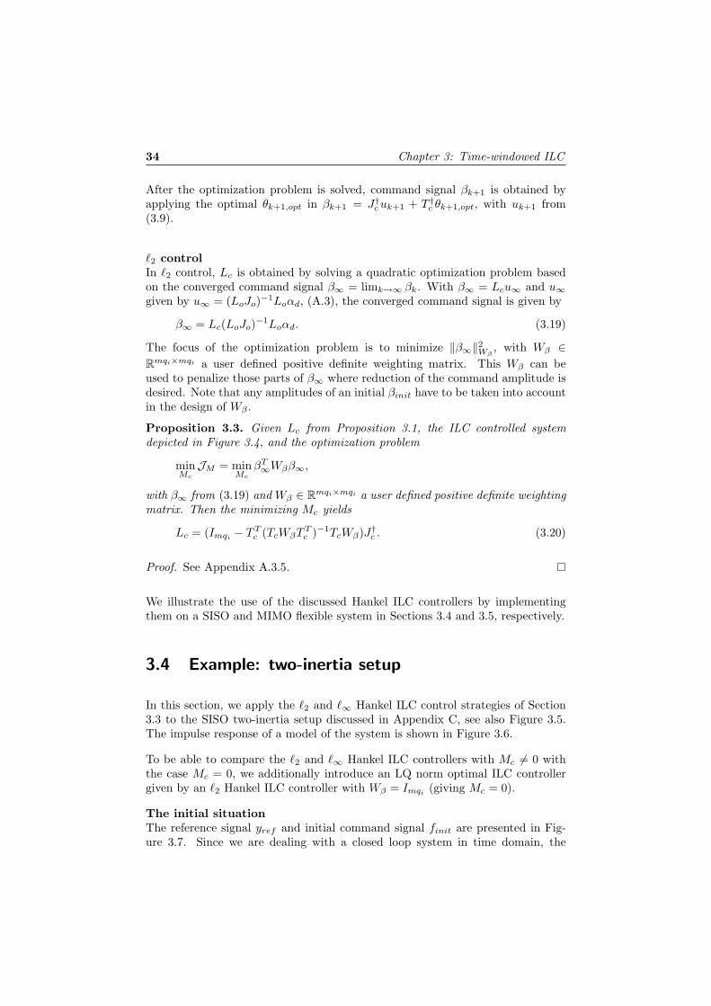
3.3: Hankel ILC control design 33

Although in general we have ε∞ 6= 0, in Chapter 4 we will show that with thisε∞ we achieved optimal performance Pε,opt, i.e. we achieved a minimized ‖ε∞‖2over all possible (Lo, Lc).

3.3.2 Step Mc: Command signal manipulation

Our goal of command signal manipulation is to reduce the larger amplitudes inthe command signal. By reducing the amplitude, we reduce the possibility ofsaturating the command signal.

We propose two approaches to reach this goal: The first one is based on minimiza-tion of the maximum amplitude of the command signal, referred to as `∞ control,[134]. The second approach is based on minimization of the weighted convergedcommand signal ‖β∞‖2Wβ

, denoted as `2 control.

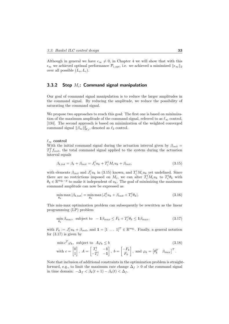
`∞ controlWith the initial command signal during the actuation interval given by βinit =TT

f finit, the total command signal applied to the system during the actuationinterval equals

βk,tot = βk + βinit = J†c uk + T †c Mcuk + βinit, (3.15)

with elements βinit and J†c uk in (3.15) known, and T †c Mcuk yet undefined. Sincethere are no restrictions imposed on Mc, we can alter T †c Mcuk to T †c θk withθk ∈ Rmqi−p to make it independent of uk. The goal of minimizing the maximumcommand amplitude can now be expressed as

minθk

max |βk,tot| = minθk

max |J†c uk + βinit + T †c θk|. (3.16)

This min-max optimization problem can subsequently be rewritten as the linearprogramming (LP) problem

minθk

βmax, subject to − 1βmax ≤ Fk + T †c θk ≤ 1βmax, (3.17)

with Fk := J†c uk + βinit, and 1 = [1 . . . 1]T ∈ Rmqi . Finally, a general notationfor (3.17) is given by

min cT ϕk, subject to Aϕk ≤ b (3.18)

with c =[01

], A =

[T †c −1−T †c −1

], b =

[−Fk

Fk

], and ϕk =

[θT

k βmax

]T.

Note that inclusion of additional constraints in the optimization problem is straight-forward, e.g., to limit the maximum rate change ∆f > 0 of the command signalin time domain: −∆f < βk(t + 1)− βk(t) < ∆f .


After the optimization problem is solved, command signal βk+1 is obtained byapplying the optimal θk+1,opt in βk+1 = J†c uk+1 + T †c θk+1,opt, with uk+1 from(3.9).

`2 controlIn `2 control, Lc is obtained by solving a quadratic optimization problem basedon the converged command signal β∞ = limk→∞ βk. With β∞ = Lcu∞ and u∞given by u∞ = (LoJo)−1Loαd, (A.3), the converged command signal is given by

β∞ = Lc(LoJo)−1Loαd. (3.19)

The focus of the optimization problem is to minimize ‖β∞‖2Wβ, with Wβ ∈

Rmqi×mqi a user defined positive definite weighting matrix. This Wβ can beused to penalize those parts of β∞ where reduction of the command amplitude isdesired. Note that any amplitudes of an initial βinit have to be taken into accountin the design of Wβ .

Proposition 3.3. Given Lc from Proposition 3.1, the ILC controlled systemdepicted in Figure 3.4, and the optimization problem

minMc

JM = minMc

βT∞Wββ∞,

with β∞ from (3.19) and Wβ ∈ Rmqi×mqi a user defined positive definite weightingmatrix. Then the minimizing Mc yields

Lc = (Imqi− TT

c (TcWβTTc )−1TcWβ)J†c . (3.20)


We illustrate the use of the discussed Hankel ILC controllers by implementingthem on a SISO and MIMO flexible system in Sections 3.4 and 3.5, respectively.

3.4 Example: two-inertia setup

In this section, we apply the `2 and `∞ Hankel ILC control strategies of Section3.3 to the SISO two-inertia setup discussed in Appendix C, see also Figure 3.5.The impulse response of a model of the system is shown in Figure 3.6.

To be able to compare the `2 and `∞ Hankel ILC controllers with Mc 6= 0 withthe case Mc = 0, we additionally introduce an LQ norm optimal ILC controllergiven by an `2 Hankel ILC controller with Wβ = Imqi

(giving Mc = 0).

The initial situationThe reference signal yref and initial command signal finit are presented in Fig-ure 3.7. Since we are dealing with a closed loop system in time domain, the

3.4: Example: two-inertia setup 35

Figure 3.5: Two-inertia setup used for the experiments.

0 0.2 0.4 0.6 0.8 1

0

0.05

0.1

time [s]

impu

lse

resp

onse

[rad

]

Figure 3.6: Impulse response of system J(z).

reference signal yd equals the initial error signal (1 + PC)−1(yref − Pfinit). Fur-thermore, from Figure 3.7, we can state that only 58 samples are used to ac-tuate the system, while 443 samples are used for observation. Consequently,we have JH ∈ R443×58. With the order of our model J equal to 7, we findrank(JH) = p = 7, Jc ∈ R7×58, and Jo ∈ R443×7.

Hankel ILC control designController Lc is based on Proposition 3.1, and Lo is designed according to LQnorm optimal ILC, (3.14), with R = rLc(LT

c Lc)−2LTc for simplicity (Note that

the inverse term in Lo corresponds to a 7×7 matrix). Subsequently, for `2 control,the weighting matrix Wβ is chosen diagonal, with

diag(Wβ) = 500|β∞ + βinit|, (3.21)

and β∞ the converged command signal (3.19) for Mc = 0. By defining Wβ as in


0 0.2 0.4 0.6 0.8 1

020406080

y ref [r

ad]

0 0.2 0.4 0.6 0.8 1−2

0

2

f init [V

]

m1

n1=m

2+1 n

2

actuation

observation

time [s]

Figure 3.7: Reference signal yref and initial command signal finit.

(3.21), the command signal is penalized most at those time instants where theo-retically β∞ has the largest amplitude. Note that this is just one possible choicefor Wβ .

Experimental resultsThe experimental results for LQ norm optimal, `2, and `∞ control strategies areshown in Figure 3.8 to Figure 3.11. The values r = 0.1 and g = 0.5 used for theexperiments are obtained experimentally.

The initial residual vibration αd during k = 0 is shown in Figure 3.8, and the errornorms ‖εk‖2 as function of trial number k are presented in Figure 3.9. Althoughthe Hankel ILC controllers are merely designed to be convergent, it can be seenthat the norms actually converge monotonically up to approximately -20dB. For‖εk‖2 < −25dB, the signals are dominated by sensor noise (the finite resolutionof the encoder).

The error signals during the observation time interval are presented in Figure 3.10.After convergence, the measured errors are in-between the optimal errors pre-sented in the left three plots of Figure 3.10, and the “worst case” convergederrors in the right three plots. The oscillations in Figure 3.10 (right) are causedby the finiteness of the encoder resolution, and the fact that the desired referenceangle of 80 rad is not an integer times the resolution. Note, however, that withthe resolution of the encoder equal to π · 10−3 rad, even the worst case errors arewithin one encoder count.

Though the error signals for all three control strategies look similar, the commandsignals clearly differ. In the top plot of Figure 3.11, the converged command sig-

3.4: Example: two-inertia setup 37

0.6 0.65 0.7 0.75 0.8 0.85 0.9 0.95 1

−0.1

0

0.1

time [s]

α d [rad

]

Figure 3.8: Residual vibration during observation interval, αd, without Hankel ILC(k = 0).

20 40−40

−30

−20

−10

0

||εk|| 2 [d

B]

LQ opt

20 40−40

−30

−20

−10

0

trial k

`2

20 40−40

−30

−20

−10

0

`∞

Figure 3.9: 2-norm of the error εk as function of trial k. Left: LQ norm optimal HankelILC. Center: `2 Hankel ILC. Right: `∞ Hankel ILC.

nals for LQ norm optimal control and `2 control are shown. Due to the chosenWβ , the `2 command signal has a maximum amplitude which is 5 percent smallerthan the LQ norm optimal command signal. In the bottom plot, LQ norm opti-mal control is compared to `∞ control. In this case, the reduction in maximumamplitude is 18 percent.


0.6 0.8 1−0.01

0

0.01

0.02

ε [r

ad]

LQ

0.6 0.8 1−0.01

0

0.01

0.02

ε [r

ad]

`2

0.6 0.8 1−0.01

0

0.01

0.02

time [s]

ε [r

ad]

`∞

0.6 0.8 1−0.01

0

0.01

0.02

LQ

0.6 0.8 1−0.01

0

0.01

0.02

`2

0.6 0.8 1−0.01

0

0.01

0.02

time [s]

`∞

Figure 3.10: Error signals εk during observation interval. Top: LQ norm optimalHankel ILC, Center: `2 Hankel ILC, Bottom: `∞ Hankel ILC. Left, top to bottom:optimal error signals after convergence (trials k = 50, k = 47, and k = 48, respectively),Right, top to bottom: worst case error signals after convergence (trials k = 48, k = 50,and k = 50, respectively).

0.5 0.52 0.54 0.56−2

−1

0

1

f 50 [V

]

m

1m

2n

1trial 50 LQ opt

`2

0.5 0.52 0.54 0.56−2

0

2

time [s]

f 50 [V

]

m1

m2

n1trial 50 LQ opt

`∞

Figure 3.11: Converged command signals for LQ norm optimal, `2, and `∞ Hankel ILC.

3.5: Example: flexible beam setup 39

Figure 3.12: The flexible beam setup used for the experiments.

0 0.2 0.4−0.1

0

0.1

sens

or 1

[mm

] actuator 1

0 0.2 0.4−0.1

0

0.1actuator 2

0 0.2 0.4−0.1

0

0.1actuator 3

0 0.2 0.4−0.1

0

0.1

sens

or 2

[mm

]

0 0.2 0.4−0.1

0

0.1

0 0.2 0.4−0.1

0

0.1

0 0.2 0.4−0.1

0

0.1

sens

or 3

[mm

]

0 0.2 0.4−0.1

0

0.1

time [s]0 0.2 0.4

−0.1

0

0.1

Figure 3.13: Impulse response of the MIMO flexible beam.

3.5 Example: flexible beam setup

In this section, we apply standard ILC (ILC for servo tasks), `2, and `∞ HankelILC to the MIMO flexible beam setup discussed in Appendix D, see also Figure3.12. The measured impulse response of the time domain feedback controlledsystem is presented in Figure 3.13.


3.5.1 ILC for servo tasks

Initial situationThe reference signal used for the servo task is presented in Figure 3.14. The totalnumber of samples in a trial is given by N = 400, and the sample time equalsTs = 1 · 10−3s.

0 0.05 0.1 0.15 0.25 0.3 0.350

0.2

0.4

0.6

0.8

1

posi

tion

[mm

]

reference

Figure 3.14: Reference signal for ILC for servo tasks.

To apply standard ILC on the setup, we first construct the convolution matrix Jusing the impulse response data of Figure 3.13. Although we could directly usethe measured impulse response to define the model J ∈ R1200×1200, due to uncer-tainty in the response (non repetitive elements such as noise), we consider onlythe first 300 singular values and directions of J for ILC control design (p = 300).Using the SVD of J , see Appendix A.3.6, we find Jc = V T

1 ∈ R300×1200 andJo = U1Σ1 ∈ R1200×300.

ILC control design and experimental resultsController Lc is based on Proposition 3.1 with Mc = 0, and Lo is designed ac-cording to (3.14), with R = rLc(LT

c Lc)−2LTc = rLcL

Tc since LT

c Lc = I300. Thevalues g = 0.5 and r = 0.01 are determined experimentally.

The error ek and command signal fk during trial k = 15 are presented in Fig-ure 3.15. Although the error norm ||ek||2 decreases as function of k, the commandsignal has an undesired signal form for Tst → 0.4s. Clearly, the ILC controllerhas problems of generating a nonzero command signal near the end of the trial.Increasing p and/or decreasing r does improve the effect near Tst = 0.4 s, butresults in less smoother command signals during the trial, or even in trial domaininstability. The fact that an increase in p reduces this effect, suggests that the sig-nal forms in J which can generate the nonzero output for Tst → 0.4s are presentin the 900 singular directions which have been removed for ILC control design.

A (pragmatic) solution for this problem is found by adding time domain inte-grators to the system, and subsequently designing a convergent trial domain ILC


2 4 6 8 10 12 1410

−2

100

||ek|| 2

||e1||2

||e2||2

||e3||2

0 0.1 0.2 0.3 0.4−0.01

0

0.01

e 15 [m

m]

e1

e2

e3

0 0.1 0.2 0.3 0.4−1

0

1

time [s]

f 15 [V

]

f1

f2

f3

Figure 3.15: Standard ILC. Top: 2-norm of the error as function of trial number.Center: Error signal during trial k = 15. Bottom: Command signal during trial k = 15.

controller for this modified time domain system. As a consequence, ILC controldesign of Lo is now based on J → JTfint

, with

Tfint=

Iqi 0...

. . .Iqi

· · · Iqi

the lifted domain representation of the time domain integrator βk(t+1) = βk(t)+∆βk(t). Furthermore, controller Lc is now given by Lc = Tfint

J†c . In this modifiedcase, the trial state uk 6= βk. Rather, uk corresponds to the rate change of thecommand signal βk, i.e., uk(t) = βk(t)− βk(t− 1).

In Figure 3.16, the error and command signal during trial 30 are shown. As canbe seen, with the time domain integrators included in the ILC controller, thecommand signal now is capable of generating the nonzero output near Tst = 0.4s.

Note that, although the reference signal is constant for Tst ∈ [0.081, 0.4]s, thecommand signal during that time interval is not constant. This can be the resultof trial varying disturbances for Tst > 0.081 s. However, due to its periodicbehavior, it is more likely that controller Lc is not capable of generating a constantcommand signal, i.e., there does not exist a linear combination of the vectors inLc such that the output is constant. This phenomenon is explained by the factthat we designed Lc using only the first 300 singular vectors of JTfint . A less


oscillatory behavior of the command signals for Tst > 0.081 s is obtained byincreasing the number of singular vectors in Lc.

0 0.1 0.2 0.3 0.4−0.01

0

0.01

e 30 [m

m]

0 0.1 0.2 0.3 0.4−1

0

1

f 30 [V

]

0.1 0.15 0.2 0.25 0.3 0.35 0.40.45

0.5

0.55

time [s]

f 30 [V

]

f1, zoomed in for t∈ [n1,n

2]

e1

e2

e3

f1

f2

f3

f1

Figure 3.16: Standard ILC with additional integrators. Top: Error signal ek duringtrial k = 30. Center: Command signal fk during trial k = 30. Bottom: Commandsignal fk during trial k = 30, zoomed in.

3.5.2 Hankel ILC design

Initial situationFor Hankel ILC, we use the reference signal shown in Figure 3.17, with actuationtime interval: m1 = 50 and m2 = 81, giving m = 32, and observation timeinterval: n1 = 82 and n2 = 400, giving n = 319. Moreover, the residual vibrationsαd for trial k = 0 are presented in Figure 3.18. Although these vibrations aredominated by a resonance of 5.5Hz (translation mode), errors e1 and e2 also showhigher frequency resonances.

The time-windowed system JH for Hankel ILC equals JH = TyJTf , with Ty givenin (3.6) and Tf defined by

Tf = Tfint

0m1qi×mqi

Imqi

0(N−m2−1)qi×mqi

. (3.22)

Since the model for J is based on measurement data, we can only estimate theorder of JH . Using the singular values of JH , see Figure 3.19, we choose p = 12.


0 0.05 0.1 0.15 0.25 0.3 0.350

0.2

0.4

0.6

0.8

1

time [s]

posi

tion

[mm

]

m1

m2

n1

n2

actuation

observation

reference

Figure 3.17: Reference signal with separated actuation and observation time interval.

0 0.05 0.1 0.15 0.25 0.3 0.35 0.4

0

0.5

1

time [s]

erro

r [m

m]

m1

n1

n2

e1

e2

e3

Figure 3.18: Residual vibration αd for the three outputs corresponds to the error signalsduring t ∈ [n1, n2].

10 20 30 40 50 60 70 80 90

−60

−40

−20

0

20

40

60

sing

ular

val

ue

← 12th singular value

Figure 3.19: Singular values of JH .


Hankel ILC control designBased on JH and p = 12, we design three Hankel ILC controllers. The three con-trollers have the same control element Lo, (3.14), with experimentally obtainedvalues g = 0.5 and R = rLc(LT

c Lc)−2LTc with r = 1 (note that LT

c Lc ∈ R12×12).Moreover, the structure of the three Lc is also chosen equal: Lc = Tfint

J†c +Tfint

T †c Mc. The Hankel ILC controllers differ in the choice for Mc.

Experimental resultsThe first controller Lc equals (3.12) with Wβ = Imqi

. The resulting error signalsas function of trial and time are presented in Figure 3.20. In accordance withHankel ILC control design, the residual vibrations during the observation timeinterval are suppressed, while the error outside the interval is not compensatedfor.

5 10 15 20 25 3010

−2

100

||εk|| 2

Wβ=I

0 0.1 0.2 0.3 0.4−0.1

00.10.20.3

e 30 [m

m]

e1

e2

e3

0 0.1 0.2 0.3 0.4−0.01

0

0.01

time [s]

e 30 [m

m]

e1

e2

e3

||ε1||2

||ε2||2

||ε3||2

Figure 3.20: Hankel ILC with Wβ = Imqi . Top: 2-norm of error εk as function of thetrial. Center: Error signal ek during trial k = 30. Bottom: Error signal ek during trialk = 30, zoomed in.

The second controller Lc is similar to the first controller, but with a Wβ given by

Wβ = diag(Iqi, . . . , 1.5Iqi

). (3.23)

The diagonal matrix in (3.23) is used to penalize the command signal amplitudes,with gain 1 for β∞(1) up to gain 1.5 for β∞(m).

The results obtained with this second controller are presented in Figure 3.21.Although the error ε30 is slightly larger than ε30 of Figure 3.20, this Hankel ILC


5 10 15 20 25 3010

−2

100

||εk|| 2

Wβ=diag(1,...,1.5)

||ε1||2

||ε2||2

||ε3||2

0 0.1 0.2 0.3 0.4−0.1

00.10.20.3

e 30 [m

m]

e1

e2

e3

0 0.1 0.2 0.3 0.4−0.01

0

0.01

time [s]

e 30 [m

m]

e1

e2

e3

Figure 3.21: Hankel ILC with Wβ of (3.23). Top: 2-norm of error εk as function of thetrial. Center: Error signal ek during trial k = 30. Bottom: Error signal ek during trialk = 30, zoomed in.

controlled system is still very capable of suppressing the residual vibrations.

Finally, the third controller is based on `∞ Hankel ILC with an additional con-straint on the rate change of the command signal: ∆f = 1 volt. The error signalsobtained with this controller are given in Figure 3.22. The error is again slightlylarger than ε30 of Figure 3.20, but still most of the residual vibrations are removed.

The differences in the size of the error signals can be explained as follows. Duringthe design of the `2 and `∞ controllers, we assumed that JHTfint

T †c = 0. Hence,we assumed that any signal JHTfint

T †c Mcuk would give an output equal to zero.In this application, however, JHTfint

T †c > 0 resulted in nonzero outputs. Conse-quently, for the cases Mc 6= 0, additional signal forms were present in the errorsignals which could not be compensated for by the Hankel ILC controller.

Based on the error results, it looks like all three controllers behave approximatelyequal. This is to be expected, since all three controllers have similar Lo andTfint

J†c . The difference between the controllers is found in Mc, and hence in thecommand signal forms applied to the system to obtain the above error signals, seeFigure 3.23. Clearly, the signal forms of the different command signals differ dur-ing the actuation time interval. After t = m2 though, all three command signalsare constant and approximately equal (in contrast to standard ILC, Figure 3.16).Furthermore, when comparing the maximum amplitude of the command signals


5 10 15 20 25 3010

−2

100

||εk|| 2

|∆

f|<1 Volt

||ε1||2

||ε2||2

||ε3||2

0 0.1 0.2 0.3 0.4−0.1

00.10.20.3

e 30 [m

m]

e1

e2

e3

0 0.1 0.2 0.3 0.4−0.01

0

0.01

time [s]

e 30 [m

m]

e1

e2

e3

Figure 3.22: Hankel ILC with minimized maximum command signal amplitude. Top:2-norm of error εk as function of the trial. Center: Error signal ek during trial k = 30.Bottom: Error signal ek during trial k = 30, zoomed in.

from the first controller with the second controller, a reduction in maximum signalamplitude of 25% is achieved. The maximum amplitude of the command signalsof the third controller is even 48% smaller than that of the first controller.

3.6 Concluding remarks

We have derived a special form of ILC, denoted by Hankel ILC, which is capableof suppressing residual vibrations in flexible systems performing point-to-pointmotions. This special form has been obtained by introducing an actuation andobservation time window in the ILC control framework. As a result, the timeinterval during a trial in which the system is actuated is separated from the timeinterval in which the measured output values used for ILC are collected.

Within a newly proposed ILC framework, we have shown that convergence of theILC controlled system can be achieved. Furthermore, we have proven that there isthe additional freedom in Hankel ILC control design to manipulate the amplitudeof the command signal, and illustrated this with experiments on flexible motionsystems.

From an input shaping point of view, Hankel ILC can be considered a new input

3.6: Concluding remarks 47

0.05 0.06 0.07 0.08−2

0

2

m1

m2

f1 (W=I)

f1 (Wβ)

f1 (∆f)

0.05 0.06 0.07 0.08−2

0

2

feed

forw

ard

f 30 [V

]

m1

m2 f2 (W=I)

f2 (Wβ)

f2 (∆f)

0.05 0.06 0.07 0.08−2

0

2

time [s]

m1

m2

f3 (W=I)

f3 (Wβ)

f3 (∆f)

Figure 3.23: Command signal f i, i = 1, 2, 3, for the three Hankel ILC controllers.

shaping technique capable of iteratively suppressing residual vibrations originat-ing from multiple modes in presence of model uncertainty. From an ILC point-of-view, Hankel ILC has resulted in a better understanding of ILC for point-to-pointmotion problems. Moreover, it has revealed the different modeling and designissues in ILC for time-windowed systems.

49

Chapter 4

ILC for systems with basisfunctions

In this chapter, we extend and formalize the results of ILC for time-windowed systems from Chapter 3 to a larger class of systems consistingof linear systems with input/output (i/o) basis functions. First, we showthat various different ILC formulations in the literature can be captured bya common system representation involving i/o basis functions. Second,analysis of this framework reveals how different ILC objectives (mono-tonic convergence, performance, minimization of input amplitudes) canbe reached by design of separate parts of the ILC controller. The analysisis subsequently expanded by studying the effects of trial varying distur-bances on performance. This results in suggestions for compensation ofthese effects. Finally, we use these results to systematically design ILCcontrollers for the representation under study, and we show that the ob-tained results are applicable to existing ILC problem formulations withi/o basis functions, and problem formulations which can be interpretedas such.

4.1 Basis functions in ILC

In this section, we show that time windows can be considered a specific class ofbasis functions. Based on this observation, in this chapter, we will extend andformalize the Hankel ILC results of Chapter 3 to the class of linear systems withbasis functions.

50 Chapter 4: ILC for systems with basis functions

Originally, in Chapter 2 we introduced an ILC framework which can be used toservo problems, Figure 4.1 (top). Subsequently, in Chapter 3 we discussed ILCfor time-windowed systems using the example of Hankel ILC. For that purpose,we included time windows (Tf , Ty) in the ILC framework, resulting in Figure 4.1(bottom).

In Figure 4.1, Tf is the matrix with input basis functions which maps the co-efficient vector βk to the command signal fk, yk equals the output signal, andαk denotes the projected output onto a space spanned by the output basis func-tions contained in matrix Ty. Furthermore, αd is the reference signal in the spacespanned by the basis functions in Ty.

Tf

ILC

ILC

J

J Tyαkβk

αd

ekfk

fk εk

yd

yk

yk

+

+

−

−

Figure 4.1: Top: Original ILC framework for servo problems. Bottom: ILC frameworkwith additional input filter Tf and output filter Ty representing, e.g., time window filters.

As mentioned, in Hankel ILC the filters (Tf , Ty) correspond to time windows.This is, however, only one possible choice for basis functions. To analyze the useof basis functions in ILC (both implicitly and explicitly), and to give examples ofinterpretations of βk, αk, and (Tf , Ty), we investigate the following systems andapplications.

Basis functions for restricted time windowsReferences [7, 66] and [76] study performance and convergence properties of sys-tems with nonzero relative degrees and delays. With the original system notsuitable for analysis, the i/o mapping of the system is reduced by removal of thefinal samples and first samples from i/o mapping, Figure 4.2, and by defining thereference signal to comply with this projected output time interval.

Basis functions for restricted command-output spaceThe authors of [50, 61, 62, 69, 132] and [138] overcome the high-dimensionalproblem of describing linear systems for ILC by capturing the i/o behavior of thesystem in a restricted i/o space. This is accomplished by describing the command

4.1: Basis functions in ILC 51

0

0

0

0

1

1

N − n

m

m

m + 1

N − 1

N − 1

N − 1

N − 1

n

n

bf

bf

bf

bf

bf

bf

coeff

com

mand

outp

ut

pro

j(outp

ut)

Figure 4.2: Top: The command signal (time signal) is constructed from a coefficientvector of length m + 1 and m + 1 unit pulse basis functions (bf) which represent thetime window. The final N −m− 1 samples of the command signal equal zero. Bottom:The output (time signal) is filtered by unit pulse basis functions to obtain a projectedoutput of length N −n. This projected output equals the output signal for time intervalt ∈ [n, N − 1].

as a linear combination of a relatively small set of basis functions (in comparisonwith the number of samples N in a trial), and by mapping the output onto areduced output space, Figure 4.3. These basis functions are a function of theoriginal reference signal and system dynamics, or are user defined. Moreover, theoriginal reference signal is mapped onto the lower dimensional projected outputspace.

0

0

0

0

0

0

0

0

1

1

3

3

N − 1

N − 1

N − 1

N − 1

N − 1

N − 1

N − 1

N − 1

bf 1

bf 1

bf 2

bf 2

bf 3

bf 3

coeff

com

mand

outp

ut

pro

j(outp

ut)

Figure 4.3: Top: The command signal (time signal) is the scaled sum of three basisfunctions (bf), with the scaling factors captured in the coefficient vector. Bottom: Theoutput signal is projected onto an output space with three components.


Basis functions for specialized tasksReferences [29, 54, 137] demand the suppression of the terminal error sample atthe end of a trial by actuating the system with a single command signal (terminalILC). This solution can be seen as the result of applying a single basis functionto construct the command signal and a time window to the output of the system,Figure 4.4. Note that in terminal ILC, the reference signal consists of only onesample.

1

00

0

0

0N − 1

N − 1N − 1 N − 1

N − 1com

mand

outp

ut

bf

bf

coeff

pro

j(outp

ut)

Figure 4.4: Terminal ILC. Top: The command signal is the result of one scaled ba-sis function, with the scaling factor captured in the coefficient vector. Bottom: Theprojected output signal equals the final time sample the output signal.

The authors [68, 142] downsample the i/o signals of the system using time win-dows to achieve specific convergence properties of the ILC controlled system, seeFigure 1.3 (bottom). In this case, the reference signal is defined using the lowersample rate.

In Chapter 3, we used ILC for residual vibration suppression in point-to-pointmotion problems. Since these problems require a system that is being actuatedduring the point-to-point motion while the residual vibrations are being measuredafter arrival at the desired position, we introduced time window based basis func-tions corresponding to actuation and observation time windows in the controlproblem, Figure 4.5. In this case, the reference signal corresponds to the desiredposition during the observation time interval.

The discussed systems and applications all have in common that the i/o behav-ior of the original system J is modified to comply with the desired ILC problemstatements. Moreover, the reference signals αd are problem dependent. Basedon these observations, in this chapter we formulate a system description whichencompasses the discussed systems and applications as special cases, and intro-duce an ILC framework suitable for this system description. Moreover, we derivean ILC analysis and design theory for systems with basis functions, based on theproposed ILC framework.

Note that the ILC framework is similar to Figure 3.4. In contrast, the derivationof the analysis and design theory is based on existing ILC control theory, however,modified such that it is applicable to the proposed ILC framework. Consequently,

4.1: Basis functions in ILC 53

PSfrag

0

0 1

1

N − 1

N − 1

N − 1

N − 1

n1

n1

n2

n2

m1

m1

m2

m2m

n

com

mand

outp

ut bf

bf

bf

bf

bf

bf

coeff

pro

j(outp

ut)

Figure 4.5: Hankel ILC: Top: The command signal (time signal) is constructed froma coefficient vector of length m = m2 −m1 + 1 and m unit pulse basis functions (bf)which represent the time window. The first m1 and final N − m2 − 1 samples of thecommand signal equal zero. Bottom: The output (time signal) is filtered by unit pulsebasis functions to obtain a projected output of length n = n2 − n1 + 1. This projectedoutput equals the output signal for time interval t ∈ [n1, n2].

the analysis and design theory is the extension of existing ILC control theory tolinear systems with basis functions.

In the discussion on the analysis and design theory for the proposed ILC frame-work, we focus on the ILC control objectives presented in Figure 4.6. As a result,in this chapter we do not focus on, e.g., robustness aspects of ILC in presence ofmodel uncertainty [43, 89], or initial condition disturbances due to errors in theresetting of the system between two trials [71, 142].

The outline of this chapter is as follows. In Section 4.2, a system description

U n d e r n o n r e p e t i t i v e d i s t u r b a n c e

N o r m - o p t i m a l i t y

M o n o t o n i c c o n v e r g e n c e

C o n t r o l o b j e c t i v e s

A d d i t i o n a l d e s i g n f r e e d o m

C o n v e r g e n c e


C o n v e r g e n c e s p e e d

Figure 4.6: ILC control objectives.


is presented which encompasses the discussed systems and applications as spe-cial cases. Moreover, we introduce an ILC framework which is suitable for thisgeneralized system. ILC control objectives in this ILC framework are analyzedfrom a system perspective in Section 4.3, yielding ILC controller conditions whichare required for convergence and optimal performance. In Section 4.4, the ILCframework is analyzed from an ILC control design perspective. This reveals howdifferent ILC objectives can be reached by design of separate parts of the ILC con-troller. Performance under trial varying disturbances is subsequently analyzed inSection 4.5, resulting in guidelines on how to reduce the effects of the trial vary-ing disturbances on performance. In Section 4.6, the obtained analysis resultsare used in the design of ILC controllers for systems with basis functions. Inaddition, practical suggestions and choices are given to facilitate straightforwarddesign. To briefly exemplify the generality of the obtained results, in Section 4.7three examples from ILC literature are discussed. And finally, concluding remarksare given in Section 4.8.

Part of the contents of this chapter is published in [128].

4.2 General ILC system description

In this section, we consider LTV systems J as given in (2.1), with f(t) ∈ Rqi thecommand signal, and y(t) ∈ Rqo the output signal. For the time span of a trialt ∈ [0, N − 1], the i/o behavior of J is represented by J of (2.3).

The discussed systems and applications in Section 4.1 all have in common thatthey modify the original system to meet the ILC problem statements. Startingwith the original system y = Jf , the manipulation of the command signal fcorresponds to f becoming a function of a new command signal β, and a matrixTf containing basis functions, i.e., f = Tfβ. Similarly, the new manipulatedoutput α is the result of the mapping of the output y onto a limited outputspace spanned by the basis functions contained in the matrix Ty, i.e., α = Tyy.Depending on the problem formulation, the basis functions correspond to timewindows, or to reference signals and user defined signals.

Let φj ∈ RNqi , j = 1, 2, . . . ,m, be the basis functions used to build the commandsignal, and θi ∈ RNqo , i = 1, 2, . . . , n, the basis functions used to define a lowerdimensional output space. These basis functions form the matrices Tf and Ty

defined by (4.1).

Tf =[φ1 φ2 . . . φm

], Tf ∈ RNqi×m,

Ty =[θ1 θ2 . . . θn

]T, Ty ∈ Rn×Nqo . (4.1)

The result of modifying the i/o behavior of the original system J using the basisfunctions is presented in Figure 4.7. The mapping H : βk 7→ αk is obtained by

4.2: General ILC system description 55

considering Tf and Ty as part of the new system H = TyJTf . Consequently, ILCcontrol design shifts from design for system J with time signals (fk, yk) to designfor system H with coefficient signals (βk, αk).

βk fk yk αk

αd

εkJ

H

Tf Ty+

−

Figure 4.7: General system H ∈ Rn×m consisting of system J and matrices Tf and Ty,with Tf and Ty containing the input and output basis functions, respectively.

The error signal εk ∈ Rn in Figure 4.7 corresponds to the difference between thereference signal αd ∈ Rn and αk ∈ Rn. As illustrated in Section 4.1, this referencesignal is problem dependent, and defined in the space spanned by Ty.

As is already demonstrated in Chapter 3, the rank of H ∈ Rn×m can be smallerthan the smallest dimension of H, i.e., p = rank(H) < min(m,n). This can becaused by the properties of J , e.g., time delays and non-minimum phase zeros,[123], or by the number and the characteristics of basis functions present in the Tf

and Ty, e.g., time windows. To properly handle these situations, decompositionof H using a full rank decomposition is essential, (4.2).

HoHc := H, αk = Hoxk, xk = Hcβk, (4.2)

with xk ∈ Rp, Ho ∈ Rn×p, Hc ∈ Rp×m, and rank(Ho) = rank(Hc) = rank(H) = pby definition.

Following the IMP reasoning of Section 3.2, we use the ILC algorithm given by

uk+1 = uk + Loεk, βk = Lcuk, u0 = 0, (4.3)

with uk ∈ Rp the trial domain state. By combining (4.2) and (4.3), we find thecontrol framework presented in Figure 4.8. Although we focus on this systemrepresentation for our ILC analysis and control design, for implementation of theframework we use Figure 4.9. Note that choosing Lim

c = TfLc makes the structureof Figure 4.9 equivalent to that of Figure 4.8.

Remark 4.1. As we have seen in Chapter 3, in the case that the basis functionsare defined by time windows, the coefficient signals βk and αk are time signals.

Remark 4.2. With H = TyJTf capturing the various ILC control problems dis-cussed in Section 4.1, we refer to H as the general system description. The explicitformulation of H as the product of two full rank matrices can be considered aminimal representation of H.

Remark 4.3. The ILC control structure of (4.3) encompasses, among others, trialinvariant ILC controllers with Arimoto gains, inverse model based ILC, and LQnorm optimal ILC.


uk+1 uk βkαk εk

αd

xkw−1Ip Lc

Lo

Hc Ho+ +

+

−

Figure 4.8: ILC framework in trial domain, with ILC controllers (Lo, Lc).

uk+1 uk fkyk εk

αd

αkw−1Ip Limc

Lo

J Ty+ +

+

−

Figure 4.9: Implementable form of the ILC framework of Figure 4.8.

4.3 ILC analysis for systems with basis functions, asystem perspective

Analysis of the ILC framework of Figure 4.8 consists of studying the different ILCcontrol objectives presented in Figure 4.6. In this section, the control objectivesare discussed from a system perspective. In Section 4.4, we discuss the objectivesfrom an ILC control design perspective. The discussion of performance undertrial varying disturbances is left for Section 4.5.

4.3.1 Convergence

Using (4.2) and (4.3), the trial domain dynamics are given by

uk+1 = (Ip − LoHLc)uk + Loαd, u0 = 0 (4.4a)

fk = Limc uk. (4.4b)

By combining the definition of monotonic convergence, Definition 2.6, and theformulation of the trial domain dynamics, (4.4), we can formulate a sufficientcondition for monotonic convergence for the proposed ILC controlled system.

4.3: ILC analysis for systems with basis functions, a system perspective 57

Lemma 4.1. Consider the ILC controlled system (4.4). Then (4.4) is convergentiff the spectral radius ρ(Ip − LoHLc) < 1, and monotonically convergent in fk if‖T−1(Ip − LoHLc)T‖i2 < 1, with T satisfying TT LimT

c Limc T = Ip.


The matrix T can be obtained by factorizing LimT

c Limc using, e.g., a Cholesky

decomposition. Lemma 4.1 states that MC of the trial state zk = T−1uk impliesMC of the command signal fk. For Lim

c = Lc = INqiand L = LoTy, the

monotonic convergence condition from Lemma 4.1 equals that of Lemma 2.1.

Finally, we refer to Section 2.3 for an interpretation of convergence speed of com-mand signal fk. Note that, as a result of the introduction of framework of Fig-ure 4.8, ‖INqi

− LJ‖i2 = κ in Section 2.3 should be replaced by ‖T−1(Ip −LoHLc)T‖i2 = κ for a proper interpretation.

4.3.2 Performance

Definition 2.7 states that performance is a function of the performance variableξk for k → ∞. Furthermore, optimal performance corresponds to the minimizedξ∞ over all stabilizing ILC controllers L, (2.11). Based on these definitions,we propose the following measures for (optimal) performance based on the ILCframework of Figure 4.8.

Proposition 4.1. Consider ILC controlled system (4.4a), and assume that (4.4a)is convergent. Furthermore, consider performance variable ξk = εk. Then perfor-mance Pε and optimal performance Pε,opt are given by (4.5) and (4.6), respec-tively.

Pε(Lo, Lc) = limk→∞

‖εk‖2 (4.5)

Pε,opt(Lo, Lc) = minLo,Lc

Pε(Lo, Lc). (4.6)

Based on Proposition 4.1, we can state the following:

Lemma 4.2. Consider ILC controlled system (4.4a), and assume that (4.4a) isconvergent. Then there exist a lower bound for Pε,opt equal to ‖(In−HoH

†o)αd‖2.

Proof. Given ε∞ = αd−Hox∞, with ε∞ = limk→∞ εk the asymptotic error. Thenoptimal performance is achieved for x∗∞ = arg minx∞ ‖ε∞‖2 → x∗∞ = H†

oαd. Asa result, the lower bound for Pε,opt equals ‖ε∗∞‖2, with ε∗∞ = (In−HoH

†o)αd.

From Lemma 4.2, we can conclude that optimal performance is reached if ε∞ ∈im(H)⊥ ∀αd ∈ Rn. In Corollary 4.1, we study the set of ILC controllers for whichPopt is reached.


Corollary 4.1. Consider ILC controlled system (4.4a), and assume that (4.4a) isconvergent. Then optimal performance Pε,opt is reached iff (Lo, Lc) ∈ (Lo, Lc) :HcLc(LoHLc)−1Lo = H†

o.

Proof. Given u∞ = (LoHLc)−1Loαd and x∞ = HcLcu∞. Then the asymptoticerror equals ε∞ = αd −Hox∞, with x∞ = HcLc(LoHLc)−1Loαd. From Lemma4.2, we know that Pε,opt requires x∗∞ = H†

oαd. Consequently, Pε,opt is reached iff(Lo, Lc) ∈ (Lo, Lc) ∈ (Rp×n, Rm×p) : HcLc(LoHLc)−1Lo = H†

o.

Note that optimal performance is a function of im(H) = im(Ho). With Ho afunction of (Tf , Ty), the number of basis functions and their characteristics bothinfluence the reachable performance.

4.4 ILC analysis for systems with basis functions, adesign perspective

In this section, we show that the different control objectives discussed in Section4.3 can be linked to different parts of the ILC controllers (Lo, Lc). To accomplishthis, Lo ∈ Rp×n and Lc ∈ Rm×p are parameterized by (4.7) and (4.8), respectively,see Figure 4.10.

Lo = SoPo, with So ∈ Rp×p and Po ∈ Rp×n (4.7)

Lc = H†cSc + T †c Mc, with Sc ∈ Rp×p, T †c = Rm×(m−p), (4.8)

and Mc ∈ R(m−p)×p arbitrary. Matrix T †c follows from the full rank decompositionT †c Tc := Im −H†

cHc. Note that, due to the definition of T †c , matrices Sc and Mc

operate in two independent subspaces.

Intuitively, the parametrization can be explained as follows. By parameterizingLo as done in (4.7), we explicitly reveal the design choices in Lo. On the one hand,we have a performance filter Po which can be chosen to pass through signals ina specific subspace, e.g., the signal forms εk ∈ im(Ho), since these signal formsare the only signals that can be compensated for by ILC anyway. On the otherhand, we obtain an additional gain matrix So which can be used for stabilizationof the ILC controlled system. The parametrization of Lc is based on the factthat the coefficient vector βk = Lcuk is divided into a part T †c Mcuk operating inthe kernel space of Hc, and a part H†

cScuk operating in the space perpendicularto ker(Hc). By design of Mc, the signal T †c Mcuk can be used to modify thespecific values in the vector βk without influencing the stability properties of theILC controlled system (since HcT

†c Mc = 0). Conversely, the signal H†

cScuk doesinfluence stability, and hence Sc is to be designed such that the ILC controlledsystem is convergent.

4.4: ILC analysis for systems with basis functions, a design perspective 59

uk+1 uk βkαk εk

αd

xk

H

Lc

Lo

w−1Ip

H†c Sc

T †c Mc

So Po

Hc Ho

+

+

+ +

+

−

Figure 4.10: ILC framework in trial domain, with parameterized ILC controllers (4.7)and (4.8).

Lemma 4.3. Given ILC controller (Lo, Lc), then there exists parameters(So, Sc, Po,Mc) such that (4.7) and (4.8) hold. Conversely, given the parameters(So, Sc, Po,Mc), then there exists (Lo, Lc) such that (4.7) and (4.8) hold.

Lemma 4.3 shows that the parametrization of (4.7) and (4.8) does not restrictdesign freedom in (Lo, Lc).

In the following sections, we discuss the relation between the parametrization ofLo and Lc and the control objectives presented in Figure 4.6.

4.4.1 Convergence

The following Lemma refines the results of Lemma 3.1.

Lemma 4.4. Consider (4.7) and (4.8) which explain how (Lo, Lc) are formed bythe choice of (So, Sc, Po,Mc). Then 1) for any given Mc, any Sc with rank(Sc) =p, and any Po with rank(PoHo) = p, there exist So such that (4.4) is monotonicallyconvergent in fk with any desired convergence speed, and 2) for any given Mc,any So with rank(So) = p, any Po with rank(PoHo) = p, there exist Sc such that(4.4) is monotonically convergent in fk with any desired convergence speed.

Proof. Follows from Lemma 3.1.

Note that the gains in Po do not restrict the gain σ(T−1(Ip−LoHLc)T ). On thecontrary, Lemma 4.4 states that after design of Po, So and Sc can be chosen suchthat σ(T−1(Ip − LoHLc)T ) has any desired gain.

Note furthermore, that the rank condition rank(PoHo) = p in the monotonic con-vergence condition imposes only a minor constraint on Po. The actual mechanism


behind Po is that it maps the signal εk ∈ im(Ho) to a lower dimensional space. InSection 4.4.2 and Section 4.5, choices for Po will be given based on performancedemands.

In Lemma 4.5, we focus on conditions for (So, Sc) which are required for assign-ment of the gain σ(T−1(Ip − LoHLc)T ).

Lemma 4.5. Let K ∈ Rp×p be chosen such that Ip − K has the desired gains,i.e., such that Ip −K is monotonically convergent with any desired convergencespeed. Furthermore, consider (4.7) and (4.8) which explain how (Lo, Lc) areformed by the choice of (So, Sc, Po,Mc). Then for any given Mc and any Po

with rank(PoHo) = p, the set of (So, Sc) for which (4.4) has gains equal to thoseof Ip −K is given by

(So, Sc) ∈ (Rp×p, Rp×p) : SoPoHoSc = TKT−1,

TT (Sc + T †c Mc)T TTf Tf (Sc + T †c Mc)T = Ip. (4.9)

Proof. Follows from substitution of (4.7) and (4.8) in Lemma 4.1.

Note that in Lemma 4.5, matrix T is a function of (Sc,Mc). Substitution of Tin SoPoHoSc = TKT−1 subsequently reveals that for given (So, Po,Mc), findingSc such that (4.4) has the desired gains requires solving a nonlinear relation inSc. On the other hand, for given (Sc,Mc), matrix T follows directly. Subsequentassignment of the desired gains by So requires solving SoPoHoSc = TKT−1,which is linear in So. Hence, gain assignment by So is more transparant and morestraightforward then gain assignment by Sc.

Corollary 4.2. Let K ∈ Rp×p be chosen such that Ip −K is monotonically con-vergent with any desired convergence speed. Furthermore, let (Sc, Po,Mc) be givenand let T follow from TT LT

c TTf TfLcT = Ip. Then So = TKT−1S−1

c (PoHo)−1

results in (4.4) which is monotonically convergent in fk and has the desired con-vergence speed.

An extreme case of convergence is deadbeat convergence, as defined in Section 4.3by ‖T−1(Ip −LoHLc)T‖i2 = 0. This case is worked out in detail in the followingCorollary.

Corollary 4.3. Consider the set of (So, Sc) of Lemma 4.5. Then the subset of(So, Sc) for which (4.4) is deadbeat, is given by

(So, Sc) ∈ (Rp×p, Rp×p) : SoPoHoSc = Ip.

Note that for deadbeat ILC control, the expression TKT−1 of Lemma 4.5 equalsIp (since K = Ip). Since Ip is not a function of T , in Corollary 4.3 we do not needto determine T .

4.4: ILC analysis for systems with basis functions, a design perspective 61

4.4.2 Performance

In Lemma 4.6, we reveal the relation between performance, as specified in Propo-sition 4.1, and the parametrization presented in (4.7) and (4.8). Consequently,Lemma 4.6 makes precise what we stated intuitively about Po in the beginningof this section.

Lemma 4.6. Consider (4.7) and (4.8) which explain how (Lo, Lc) are formed bythe choice of (So, Sc, Po,Mc). Then for any (So, Sc) for which (4.4) is convergent,and for any Mc, 1) performance is a function of Po only, i.e., does not depend onthe specific choice of (So, Sc,Mc), and 2) optimal performance is achieved withPo = HT

o .


The choice Po = HTo in Lemma 4.6 is not unique. Indeed, optimal performance

is achieved for any Po satisfying Po : (PoHo)−1Po = H†o.

We have discussed monotonic convergence and performance as ILC control ob-jectives. These objectives turn out to be separately attainable by the choice ofmatrices (So, Sc) to obtain monotonic convergence, and Po to obtain performance.As a result, there is considerable design freedom left, to be appointed to a yetundefined control objective. As we will show next, for the parametrization (4.7)and (4.8), this freedom is found in the choice for Mc.

4.4.3 Additional design freedom:exploiting command non-uniqueness

Lemma 4.7. Consider (4.7) and (4.8) which explain how (Lo, Lc) are formedby the choice of (So, Sc, Po,Mc). Then the choice for Mc ∈ R(m−p)×p neitherinfluences the monotonic convergence objective, nor the performance objective.

Proof. Follows from Lemma 4.4 and Lemma 4.6.

The additional design freedom in the ILC control framework in Figure 4.8 is dueto the fact that the map between βk and αk has a low rank. That Mc does notinfluence αk is due to the fact that HT †c Mc = 0 for all Mc. An example of whenMc 6= 0 is useful can be found in Section 3.3.

In Proposition 4.2, we extend the results of Proposition 3.3.


Proposition 4.2. Given Lc from (4.8), the ILC controlled system (4.4), andoptimization problem minMc βT

∞Wββ∞, with β∞ = limk→∞ βk and Wβ ∈ Rm×m

a user defined positive definite weighting matrix. Then the minimizing value Mc

yields

Lc = (Im − TTc (TcWβTT

c )−1TcWβ)H†cSc.

4.4.4 ILC for systems with basis functions

The complete ILC control design procedure for systems with basis functions iscaptured in Result 4.1.

Result 4.1. Design of an ILC controller for systems with basis functions is real-ized by separate design of (So, Sc), Po, and Mc, in which the ILC control objectivesmonotonic convergence, performance, and coefficient vector amplitude reductioncan be achieved, respectively. Design freedom in (So, Sc) is discussed in Lemma4.5 and Corollary 4.2, freedom in Po in Lemma 4.6, and freedom in Mc in Propo-sition 4.2.

Note that the original problem formulation in Figure 4.8, which deals with con-vergence only, shows a symmetry in its structure in the sense that the dual systemresulting from H → HT , Lc → LT

o , and Lo → LTc shows identical convergence

properties. This symmetry is actually lost in later steps by introducing additionalobjectives like monotonic convergence, performance, and minimization of inputamplitudes. This motivates to use a non-symmetrical parametrization (4.7) and(4.8).

4.5 Analysis of trial varying disturbances

To extend the previously obtained results, in this section we assume that trialvarying output disturbances dk are present in the ILC controlled system. Thesource of the disturbance is assumed to be either stochastic, e.g., measurementnoise, or deterministic, e.g., vibrations from neighboring rotating systems.

Including trial varying output disturbance dk into the ILC control framework ofFigure 4.8 results in Figure 4.11. The trial dynamics of Figure 4.11 are subse-quently given by

uk+1 = (Ip − LoHLc)uk + Lo(αd − dk), u0 = 0. (4.10)

Since dk is an external disturbance, it does not influence the convergence prop-erties of the ILC controlled system. It does, however, influence performance. Inthe following, we discuss the influence of both stochastic and deterministic dis-turbances on performance.

4.5: Analysis of trial varying disturbances 63

uk+1 uk βkαk εk

αddk

xkw−1Ip Lc

Lo

Hc Ho+ ++ +

+

−

Figure 4.11: ILC framework in trial domain, including trial varying disturbances dk.

4.5.1 Stochastic disturbances dk

The stochastic disturbance that we consider is trial domain white noise d withEd = 0 and covariance matrix EddT = Rdd. Furthermore, we assume αd anddk to be independent. The trial domain dynamics and error equal

uk+1 = (Ip − LoHLc)uk + Lo(αd − dk) (4.11a)εk+1 = αd − dk+1 −HLcuk+1. (4.11b)

To study the influence of stochastic dk on the performance, we focus on theasymptotic value for Eε∞ and the covariance Rεε = limk→∞Rεε,k with Rεε,k =E(εk−Eεk)(εk−Eεk)T . Consequently, we assume that (4.11) is convergent.

Due to linearity and Ed = 0, Eε∞ is not affected by dk. Moreover, thecovariance matrix Rεε is given by

Rεε = Rdd + HLcRuuLTc HT (4.12)

0 = Ruu − (Ip − LoHLc)Ruu(Ip − LoHLc)T − LoRddLTo , (4.13)

where (4.13) is a discrete Lyapunov equation.

In Lemma 4.8, we study the influence of convergence speed on the value of Rεε.

Lemma 4.8. Given ILC controlled system (4.11), ILC controller (4.7) and (4.8)which explain how (Lo, Lc) are formed by the choice of (So, Sc, Po,Mc), any Po

with rank(PoHo) = p, and any Mc. Furthermore, let (So, Sc) be given by So =g(PoHo)−1 with g ∈ (0, 2) and Sc = Ip, i.e., let the singular values of the ILCcontrolled system equal |1− g|Ip. Then for

g ↓ 0 : ‖Rεε‖i2 ↓ ‖Rdd‖i2

g = 1 : Rεε = Ho(HoPo)−1PoRddPTo (HoPo)−1T

HTo + Rdd

g ↑ 2 : ‖Rεε‖i2 ↑ ∞.



From Lemma 4.8, we can conclude that near zero convergence speed (g ↓ 0) resultsin Rεε in which Rdd appears unfiltered. Furthermore, with deadbeat ILC (g = 1),we find Rεε = 2Rdd for disturbances dk which lie in the space Ho(HoPo)−1Po.Finally, for g ↑ 2, the effects of dk on Rεε are clearly disastrous. Note that theseresults confirm the frequency domain performance results in [21], but contradictthe results given in [93].

Remark 4.4. Po can be chosen to deviate from the optimal solution Po = HTo ,

Lemma 4.6, if the contribution of dk in a specific direction is larger than thatof αd. For example, consider the vector αd whose elements along the vector aredominated by relatively low frequencies, and the vector dk whose elements alongthe vector are dominated by relatively higher frequencies. Then we can choosePo = HT

o Q, with Q a Toeplitz matrix in the coefficient space describing the be-havior of a zero phase low pass filter, to filter out dk from the error signal εk.Although optimal performance, as given in Lemma 4.6, is not achieved, perfor-mance reduction in αd is compensated for by less performance loss due to dk.

4.5.2 Deterministic trial periodic disturbances dk

The considered deterministic trial periodic disturbances are defined by dk(`) ∈ Rn:

dk(`) : dk+` = dk, with ` ≥ 2,

with ` representing the trial periodicity of the disturbance. Using the trial shiftoperator w, this equals dk+` = w`dk = dk. As an example of such a disturbance,consider a sinusoidal disturbance signal with a period time of 0.2 seconds, and anILC controlled system with a trial length of 0.45 seconds (including the resettingof the system between two trials). Then the ILC controlled system will encounterthe same sinusoidal disturbance every four trials (` = 4), see Figure 4.12.

0 0.5 1 1.5 2−1.5

−1

−0.5

0

0.5

1

1.5

time [s]

dist

urba

nce

k=0 k=1 k=2 k=3 k=4

Figure 4.12: Sinusoidal disturbance with period time of 0.2s, and time interval of atrial of 0.45s. During trial k = 4, the disturbance is equal to that during trial k = 0.

4.5: Analysis of trial varying disturbances 65

Note that for dk with known period `, the internal model principle, [47], can beused in the ILC controller design to asymptotically reject the periodic disturbance.In this section, however, we assume ` to be unknown, and use the ILC controllergiven in (4.3).

The trial domain behavior of the asymptotic error of an ILC controlled systemwith deterministic disturbance dk(`) can be given by

εask = ε∞ − (I −HLc(wI − Ip + LoHLc)−1Lo)dk(`), (4.14)

with ε∞ = (I −HLc(LoHLc)−1Lo)αd, and w = ej2π/`. In (4.14), we substitutedw−1 = 1 for trial invariant αd (` = 1).

In Lemma 4.9, we study the effects of convergence speed and trial periodicity `on εas

k .

Lemma 4.9. Given (4.14) with deterministic trial periodic disturbance dk(`) with` ≥ 2, ILC controller (4.7) and (4.8) which explain how (Lo, Lc) are formed bythe choice of (So, Sc, Po,Mc), any Po with rank(PoHo) = p, and any Mc. Let(So, Sc) be given by So = g(PoHo)−1 with g ∈ (0, 2) and Sc = Ip, i.e., let thesingular values of the ILC controlled system equal |1− g|Ip. Then for

g ↓ 0 : εask ≈ ε∞ − dk(` ≥ 2)

g = 1 : εask ≈ ε∞ − (Ip −Ho(HoPo)−1Po)dk(` →∞)

εask = ε∞ − (Ip + Ho(HoPo)−1Po)dk(2)

g ↑ 2 : εask ≈ ε∞ − (Ip −Ho(HoPo)−1Po)dk(` →∞)‖εas

k ‖2 →∞ for dk(2).


From Lemma 4.9, we can conclude that, independent of the trial periodicity `of dk(`), εas

k is approximately equal to ε∞ − dk for ILC controllers with nearzero convergence speed. On the other hand, with, e.g., deadbeat control, theattenuation or amplification of the disturbance does depend on the value of `.

To illustrate these results, consider H = 1, Lc = 1, and Lo = g, with g ∈ (0, 1]the tuning parameter used to influence convergence speed. For g ↓ 0, we havearbitrarily slow convergence, for g = 1 we have deadbeat control. In Figure 4.13,we show the amplitude |εas

k (`)| = |(1−(ej2π/`−1+g)−1g)| as function of ` (trial).Clearly, independent of the value for g, trial invariant disturbances (` → ∞)are fully rejected. On the other hand, it depends on the trial periodicity of thedisturbance (`), whether slow convergence or deadbeat control provides the bestdisturbance rejection.


0 0.1 0.2 0.3 0.4 0.50

0.5

1

1.5

2

1/trial

|εkas

(tria

l)|

g=1g=0.5g=0.1

Figure 4.13: Effect of tuning gain g on asymptotic amplitude rejection of trial periodicdisturbance.

4.6 ILC controller design for systems with basis func-tions

In this section, we discuss the design of ILC controllers for systems with ba-sis functions by choosing a specific full rank decomposition for H and defining(So, Sc, Po,Mc). Thereto, we apply the results of the previous sections as sum-marized in Figure 4.14. Note that the only (possibly) conflicting control ob-jectives correspond to convergence speed and performance under trial varyingdisturbances.

U n d e r n o n r e p e t i t i v e d i s t u r b a n c e ( S o , S c )

N o r m - o p t i m a l i t y ( P o )

M o n o t o n i c c o n v e r g e n c e ( S o , S c )

C o n t r o l o b j e c t i v e s

A d d i t i o n a l d e s i g n f r e e d o m ( M c )

C o n v e r g e n c e


C o n v e r g e n c e s p e e d ( S o , S c )

Figure 4.14: ILC control objectives as function of (So, Sc, Po, Mc).

Before an ILC controller can actually be designed, we first need a full rank decom-position of H. Due to the properties of a SVD, see Appendix A.3.6, we suggest

4.6: ILC controller design for systems with basis functions 67

to use SVD of H to find Ho and Hc.

With Ho and Hc given, ILC control design of (Lo, Lc) can be accomplished bydesign of (So, Sc, Po,Mc). Using Proposition 4.2, the general structure of the ILCcontroller is given by

Lo = SoPo, Lc = (Im − TTc (TcWβTT

c )−1TcWβ)H†cSc.

As a result, the design freedom in Mc is represented by design freedom in Wβ .

Sc: As a result of Lemma 4.5, we leave the assignment of σ(T−1(Ip − LoHLc)T )to So, and choose Sc = Ip.

Po: If trial varying disturbances are not taken into account in the ILC controllerdesign, or are fully unknown, Lemma 4.6 states to design Po = HT

o for optimalperformance. In case trial varying disturbances are considered, we can alter Po

to Po = HTo Q, with Q a matrix which filters out the unwanted disturbances, e.g.,

a filter with low pass characteristics, see Section 4.5.

Wβ : Reduction of the amplitudes of the values in the coefficient vector β∞ cor-responds to the design of Wβ , see Proposition 4.2. An initial estimate of theamplitudes in β∞ can be obtained by using the analytical expression for β∞ withWβ = Im: β∞(Wβ = Im) = H†

c (PoHo)−1Poαd. Now, one possible suggestionfor Wβ is to choose Wβ = gβdiag(|β∞(Wβ = Im)|) with gβ ∈ R > 0 a tuninggain. For this choice of Wβ , the larger amplitudes in β∞ are penalized more thanthe smaller amplitudes. Note that in general, however, design and tuning of Wβ

remains an iterative process.

So: Finally, we design So. A first design choice for So is given by deadbeat ILC,Corollary 4.3: So = (PoHo)−1. To be able to modify the convergence speed ofthis inverse model ILC controller, we can additionally introduce a tuning gaing ∈ (0, 2) in So, yielding So = g(PoHo)−1. The effects of g on convergence speedand trial varying disturbances is discussed in Section 4.5.

In case the smaller singular values in Ho are uncertain, we can apply a Tikhonovinverse of PoHoT , which for a different case was suggested by [12], with tuningparameters g ∈ (0, 2) and r ≥ 0

So := gT (TT HTo PT

o PoHoT + rI)−1TT HTo PT

o →I − T−1SoPoHoT = (1− g)I + rg(TT HT

o PTo PoHoT + rI)−1.

With the singular values σi(rg(TT HTo PT

o PoHoT +rI)−1) < g (since σi(PoHoT ) >0 ∀i ∈ [1, p]), we find that monotonic convergence of (4.4) is guaranteed withthis So. While parameter g can be used to alter the overall convergence speed,parameter r can be used to alter the convergence speed of the smaller gainsin the PoHoT . For σi(PoHoT ) r we find rg(TT HT

o PTo PoHoT + rI)−1 ↑ g.

This can subsequently result in arbitrarily slow convergence, see Section 4.3. Forσi(PoHoT ) r, we find rg(TT HT

o PTo PoHoT + rI)−1 ≈ 0 and a convergence

speed of |1− g|.


4.7 Reconsideration of basis function based ILC ap-proaches in ILC literature

To illustrate that the results of this chapter are directly applicable to variousILC problems, we present three distinct ILC problem formulations with basisfunctions. Thereby, we focus on reformulating the ILC control problems to complywith the framework discussed in this chapter.

4.7.1 Arimoto gains for systems with nonzero relative degrees

In [86], Arimoto gains are applied to control an LTI system with a relative degreeequal to one. For that purpose, the original system is modified using time windowbased basis functions, (4.15).

Tf =[IN−1

0

], Ty =

[0 IN−1

]→ H =

CB 0...

. . .CAN−2B . . . CB

, (4.15)

with HN−1×N−1. Since [86] assumes full rank of H, the minimal realization of Hcan correspond to (Ho,Hc) = (H, IN−1). Furthermore, the input βk and outputαk of H correspond to βk(t) = fk(t) and αk(t) = yk(t + 1) with t ∈ [0, N − 2],respectively.

The applied ILC control strategy corresponds to fk+1(t) = fk(t) + gek(t + 1) →βk+1 = βk + gεk, with 0 < g ≤ 2(CB)−1 the Arimoto gain. Formulation of thisILC control strategy in terms of (Lo, Lc) gives (gIN−1, IN−1). With Lo = SoPo,we can find So = g(HT )−1 and Po = HT .

4.7.2 Inverse model based ILC for systems with a reduced input-output space

In [132], ILC is used for a system with a reduced input space. Given an originalreference signal r ∈ RN , the matrix with input basis functions equals

Tf =[r r r(3) r(4)

], (4.16)

resulting in the modified system H = JTf ∈ RN×4 → (Ho,Hc) = (H, I4). Whileαk = yk, the input is modified from fk to coefficient vector βk ∈ R4.

System H is controlled using an inverse model based ILC controller with (Lo, Lc) =(g(HT H)−1HT , I4) and g ∈ (0, 2). Using (4.7), we obtain So = g(HT H)−1 andPo = HT .


4.7.3 ILC for residual vibration suppression

In Chapter 3, we applied ILC to suppress residual vibrations in systems per-forming point-to-point motions. With the generalized system H = JH discussedextensively in Chapter 3, here we focus on the properties of the ILC controller.

To control H, we designed an ILC controller Lo with

(Po, So) = (HTo , g(HT

o Ho + rIp)−1), g ∈ (0, 2), r ≥ 0,

and an Lc with Sc = Ip. With ker(H) 6= ∅, we used the additional design freedomMc to reduce the amplitude of the command signal.


Basis functions appear in ILC in various ways. In this chapter, we broughttogether these appearances in one system description and ILC framework. Inaddition, we have presented a general system solution for this framework, andprovided results on monotonic convergence, performance, minimization of inputamplitudes, and disturbance rejection.

The derivation of the analysis and design theory for this ILC framework hasextended existing ILC control theory such that it is applicable to the proposed ILCframework. From a system perspective, analysis of ILC control objectives in thisframework has yielded ILC controller properties which are required for monotonicconvergence and optimality of performance. Since these conditions have beendefined as function of the system properties, they apply to any ILC controllerfitting the proposed framework. From an ILC control design perspective, analysishas revealed how the ILC objectives given by monotonic convergence, optimalityof performance, and minimization of input amplitudes, can be reached by designof separate parts of the ILC controller. Analysis has furthermore shown thatconvergence speed and performance under trial varying disturbances are the onlytwo possibly conflicting control objectives.

The obtained analysis results have been used in the design of ILC controllersfor systems with basis functions. In addition, practical suggestions and choiceshave been given to facilitate straightforward ILC control design. Finally, we haveshown that the obtained results are applicable to ILC problems formulations withbasis functions, and problem formulations which can be interpreted as such.

71

Chapter 5

ILC for uncertain systems:Robust convergence analysis

In this chapter, we discuss a Robust Monotonic Convergence (RMC)analysis approach for ILC for uncertain systems over a finite time in-terval. For this purpose, a finite time interval representation of an un-certain system description is introduced. This model is subsequently usedin an RMC analysis based on µ analysis. As a result, we are capable ofhandling additive and multiplicative uncertainty models in the RMC prob-lem formulation, analyze RMC of linear time invariant MIMO systemscontrolled by any linear trial invariant ILC controller, and formulate ad-ditional straightforward RMC conditions for ILC controlled systems. Toillustrate the derived results, we analyze the RMC properties of LQ normoptimal ILC.

Introduction

The expression “uncertain system” can be interpreted in multiple ways. Oneinterpretation is to consider model uncertainty as the difference between a modeland a specific system, resulting in one specific, fixed, model error. If we assumethat measurement data of the impulse response of the system is available, thenthis model uncertainty corresponds to the difference between the true impulseresponse and that of the model. While ILC control design can be based on amodel of the system, convergence analysis can be based on the true system, i.e.,on measurement data.

72 Chapter 5: ILC for uncertain systems: Robust convergence analysis

In this chapter and in Chapter 6, however, we consider the uncertain systemto correspond to a nominal model together with an uncertainty set. The truesystem is assumed to lie somewhere in this set. In contrast to the previous modeluncertainty interpretation, in this case no explicit system response is available. Asa result, we can not use it to analyze the ILC controlled system. What we can do(and will do), is to analyze the convergence properties of the complete uncertainmodel set. With the true system assumed to be captured in this set, convergenceof each system in the set results in convergence of the true ILC controlled system.

The outline of this chapter is as follows. We introduce the uncertain systemdescription over a finite time interval in Section 5.1. Subsequently, the robustmonotonic convergence objective is defined in Section 5.2, and tackled in Section5.3. In Section 5.4, we work out the obtained robust monotonic convergenceconditions for three specific uncertainty models. We introduce basis functionsinto the analysis in Section 5.5. To illustrate our findings, in Sections 5.6 and 5.7we analyze the robustness properties of LQ norm optimal ILC. This chapter endswith concluding remarks in Section 5.8.

Part of the contents of this chapter is published in [43].

Definition. The induced 2-norm of a discrete time transfer function P (z) is givenby ‖P (z)‖i2 = maxθ∈[−π,π] σ(P (ejθ)) with θ real valued.

5.1 Uncertain system description

The focus of this chapter is on analysis of the robust convergence properties ofILC controlled systems over a finite time interval with systems that are uncertain.The finite time interval system representations follow from infinite time systemdescriptions. The infinite time systems under study are assumed to be defined by areal rational discrete time transfer function P (z), which can be causal or noncausalin the shift operator z. Given a time signal y(t), z is defined as y(t + 1) = zy(t).Consequently, P (z) has discrete time domain inputs and outputs defined over thetime axis t ∈ (. . . ,−2,−1, 0, 1, 2, . . .).

Restriction of an infinite time mapping P (z) to a finite time interval t ∈ [0, N −1]is achieved in two steps. First, observe that the mapping P (z) is equivalent tothe mapping given by the infinite dimensional convolution matrix P∞, with P∞ ablock Toeplitz matrix filled with the impulse response (Markov parameters) p(t)of P (z). Second, truncate the infinite matrix P∞ such that it describes the i/omapping for time interval t ∈ [0, N − 1], see, e.g., [20].

The finite time interval model J∆ for our uncertain system is obtained by followingthe uncertain system modeling steps as used in infinite time robust control theory,e.g., Section 7.2 of [117], Section 9.1 of [143], see Figure 5.1. In Figure 5.1, theinfinite time uncertain system J∆(z) : f(z) ∈ Cqi 7→ y(z) ∈ Cqo consists of a

5.1: Uncertain system description 73

nominal model J(z) which is assumed to be causal, and the filters (Wi(z),Wo(z))which are user defined. (Wi(z),Wo(z)) describe the specific uncertainty of thesystem under study, and are designed such that they are stable causal filterswhose inverses are again stable and causal. The ∆(z) (with ∆(ejθ) ∈ Cq×q) is acausal system with known structure, see Sections 7.3 and 7.4 of [117]. Moreover,∆(z) is assumed to satisfy ‖∆(z)‖i2 ≤ 1, i.e., ∆(z) is assumed to be normalized.As a result, the set of uncertain systems Πz is given by

Πz =J∆(z) : J∆(z) = J(z) + Wi(z)∆(z)Wo(z), ‖∆(z)‖i2 ≤ 1,

∆ structured, (5.1)

Wo(z) Wi(z)∆(z)

f(z)J(z)

∆J(z)

y(z)

Wo Wi∆

fJ

∆J

y++

++

Figure 5.1: Top: infinite time uncertain system J∆(z), consisting of a nominal modelJ(z) and additive model uncertainty ∆J(z). Bottom: uncertain system J∆ over a finitetime interval.

For given infinite time system J∆(z), the finite interval mapping J∆ ∈ RNqo×Nqi

maps the input signal f ∈ RNqi to the output signal y ∈ RNqo . Furthermore, withJ(z) causal and LTI, the system matrix J ∈ RNqo×Nqi is a lower triangular blockToeplitz matrix. Equally, the finite interval representations of (Wi(z),Wo(z))are given by the lower triangular block Toeplitz matrices Wi ∈ RNqo×Nq andWo ∈ RNq×Nqi .

With ∆(z) causal and LTI, its i/o behavior for a finite time interval can beexpressed by a lower triangular block Toeplitz matrix ∆ ∈ RNq×Nq. Moreover, forfinite dimensional lower triangular (block) Toeplitz matrices we find that ‖∆‖i2 ≤‖∆(z)‖i2, see Section 6.4 of [20], i.e., the induced 2-norm of a finite interval lowertriangular (block) Toeplitz matrix can never exceed the 2-norm of the underlying


transfer function. Consequently, the set of uncertain systems over a finite timeinterval, Π, can be given by

Π = J∆ : J∆ = J + Wi∆Wo,∆ ∈ ∆, (5.2)

where ∆ = ∆ ∈ RNq×Nq : ‖∆‖i2 ≤ 1,∆ structured.

Remark 5.1. Although the set of uncertain systems Π is derived by assuming ∆to be LTI, in Section 5.4 we show that for given LTI mappings (J,Wi,Wo), ∆can also be chosen to be linear time varying (LTV). In that case, we do haveto assume that the LTV mapping Wi∆Wo properly captures the finite intervalmodel uncertainty of the system.

Remark 5.2. To fit multiplicative uncertainty models into the additive uncertaintydescription of (5.2), define Wi = W o

i and Wo = W oo J for output multiplicative

uncertainty (I+W oi ∆W o

o )J , and Wi = JW ii and Wo = W i

o for input multiplicativeuncertainty J(I + W i

i ∆W io). For singular J , the modification from multiplicative

uncertainty to additive uncertainty results in rank deficient Wi or Wo.

As we will show in Section 5.3, the norm-bounded uncertainty ∆ is the key elementin the uncertain system description, since it allows the use of well developed robustcontrol theory for the robust convergence analysis.

5.2 Robust Monotonic Convergence objective

In this section, the concept of robust monotonic convergence of ILC for uncertainsystems is introduced, based on the ILC control framework consisting of an un-certain system J∆ and ILC controller (Q, Lo, Lc), as depicted in Figure 5.2. InFigure 5.2, p = rank(J) and ek = yd − J∆fk. Introduction of basis functions inthe ILC framework is left for Section 5.5.

Note the additional ILC filter Q in Figure 5.2. This filter is referred to as robust-ness filter, since it can be used to increase the robustness properties of the ILCcontrolled system. In this chapter, we show that, depending on the amount ofmodel uncertainty, Q 6= Ip is indeed required to obtain robustness against modeluncertainty. In frequency domain ILC control strategies, Q is often defined as azero phase low pass filter. In Arimoto gain ILC, it is common to take Q = gIp

with g ≤ 1. Q design in LQ norm optimal ILC is discussed in 5.6.

As shown in Figure 5.2, we will consider the ILC control strategy (Q, Lo, Lc) givenby

uk+1 = Quk + Loek, fk = Lcuk, u0 = 0, (5.3)

with (Q, Lo, Lc) ∈ (Rp×p, Rp×Nqo , RNqi×p).

5.2: Robust Monotonic Convergence objective 75

uk+1 uk ekfk

yd

J∆

ILC

pkqk

ykw−1Ip Lc

Lo

J

Wo Wi∆

Q

+++ +

+

−

Figure 5.2: ILC control framework in trial domain, with ILC controller (Q, Lo, Lc).

Substitution of ek = yd − J∆fk in (5.3) subsequently results in the trial domainbehavior

uk+1 = (Q− LoJ∆Lc)uk + Loyd (5.4)fk = Lcuk,

with u0 = 0.

The ILC controlled system represented by (5.4) is called robustly convergent (RC)in trial domain iff ρ(Q − LoJ∆Lc) < 1 ∀J∆ ∈ Π. Although this condition isnecessary and sufficient for convergence of (5.4), mere convergence of (5.4) canlead to undesirable transient behavior of the input and error signal norms in trialdomain, [76], e.g., the 2-norm or the maximum amplitude of the time signalsduring a trial can become unacceptably high (they can become harmful to thesystem). To avoid this undesirable behavior, (5.4) is required to be monotonicallyconvergent.

We consider two definitions for monotonic convergence: Monotonic convergenceof (5.4) with J∆ replaced by J , i.e., ∆ = 0, as defined by Definition 2.6, androbust monotonic convergence of (5.4) for J∆ ∈ Π.

Definition 5.1 (Robust Monotonic Convergence (RMC)). Given the ILC con-trolled system (5.4) and ILC controller (5.3), with yd = 0 and u0 ∈ Rp. Then(5.4) is robustly monotonically convergent (RMC) in fk if there exists 0 ≤ κ < 1such that

‖fk+1‖2 < κ‖fk‖2, ∀u0 ∈ Rp and ∀J∆ ∈ Π,

and ‖fk+1‖2 = ‖fk‖2 only for fk = fk+1 = 0.

Remark 5.3. We derive the RMC condition based on Definition 5.1. Alternatively,the same RMC condition can be found by considering yd 6= 0 and u0 = 0. Theonly difference between the two approaches is found in the definition of RMC.


For yd 6= 0 and u0 = 0, robust monotonic convergence requires ‖fk+1 − f∞‖2 <‖fk − f∞‖2 ∀J∆ ∈ Π with f∞ = limk→∞ fk.

Finally, we extend the optimal performance result of Lemma 2.2 to the ILC frame-work presented in Figure 5.2.

Lemma 5.1. Given a robustly convergent system (5.4) with asymptotic error e∞.Then e∞ = 0 for any yd iff rank(J∆) = Nqo ∀J∆ ∈ Π and Q = Ip.

Proof. Follows the proof of Lemma 2.2, with e∞ = (INqo− J∆Lc(Ip − Q +

LoJ∆Lc)−1Lo)yd.

5.3 Robust Monotonic Convergence conditions

Now that the RMC problem is defined, we tackle it for given uncertain systems(J,Wi,Wo) and ILC controller (Q, Lo, Lc). For comparison with frequency domainRMC results from ILC literature, we include an RMC condition based on transferfunction notations.

5.3.1 RMC condition

Using Definition 5.1 and Lemma 4.1 with H → J∆, we can formulate the followingsufficient RMC condition.

Corollary 5.1. Consider the ILC controlled system (5.4) with yd = 0. Fur-thermore, let T satisfy TT LT

c LcT = Ip. Then (5.4) is RMC in fk if ‖T−1(Q −LoJ∆Lc)T‖i2 < 1 ∀J∆ ∈ Π.

Proof. Follows the proof of Lemma 4.1.

At this point, it is useful to bring the one trial shift operator w−1Ip into a formatwhich is compatible with our uncertainty description. This is done in the followingProposition.

Proposition 5.1. Let T = Ip and ∆P ∈ ∆P = δP Ip : δp ∈ C, |δP | < 1.Then RC of system (5.4) of Figure 5.2 is equivalent to RC of the system inFigure 5.3. Furthermore, let T satisfy TT LT

c LcT = Ip and ∆P ∈ ∆P with∆P = ∆P ∈ Cp×p, ‖∆P ‖i2 < 1, i.e., ∆P normalized and unstructured. ThenRMC of system (5.4) of Figure 5.2 in fk is equivalent to RMC of the system inFigure 5.3 in zk.


5.3: Robust Monotonic Convergence conditions 77

PSfrag

fk

pkqkzk+1

yk

zk

Wo Wi

Lc

∆

T

J

M

Lo

Q

T−1

∆M

∆P

+ ++

+

−

Figure 5.3: M∆M structure.

Proposition 5.1 makes it possible to study the convergence properties of (5.4) byanalyzing the properties of M in Figure 5.3. System M is given by[

qk

zk+1

]=

[0 WoLcT

−T−1LoWi T−1(Q− LoJLc)T

]︸︷︷︸

M

[pk

zk

], (5.5)

and the corresponding norm bounded uncertainty set ∆M by

∆M = ∆M = diag(∆,∆P ) : ∆ ∈ ∆,∆P ∈ ∆P . (5.6)

Based on the M∆M structure of Figure 5.3, a sufficient condition for monotonicconvergence of M∆M is given by ‖M∆M‖i2 < 1. While an unstructured ∆M

would result in the arbitrarily conservative RMC condition ‖M‖i2 < 1, exploita-tion of the structure in ∆M using µ analysis can result in less conservative RMCresults. More specifically, based on the results of µ analysis in [103], it can bestated that (5.5) is RMC if µ∆M

(M) < 1, with µ∆M(M) defined by

µ∆M(M) = min

∆M∈∆M

σ(∆M ) : det(I −M∆M ) = 0−1. (5.7)

If there exists no ∆M ∈ ∆M such that det(I −M∆M ) = 0, then µ∆M(M) := 0.

Remark 5.4. Because the formulations in [103] are defined for matrices, i.e., arenot related to any application, the results are directly applicable to our system,without any restrictions.

With µ∆M(M) in general difficult to determine directly, we use an upper bound

for µ∆M(M) to derive the RMC condition for M , Proposition 5.2.


Proposition 5.2. Given system M of (5.5) with M real valued. Then an upperbound for µ∆M

(M) is given by

µ∆M(M) ≤ inf

DM∈DM

‖D1/2M MD

−1/2M ‖i2, (5.8)

with DM = DM = diag(D,DP ) : rank(DM ) = Nq + p, DM ∈ R(Nq+p)×(Nq+p),D

1/2M ∆M = ∆MD

1/2M .

Proof. The upper bound is suggested in Section 4 of [45]. The properties of DM

follow from Section 3 and Theorem 9.10 of [103].

From Proposition 5.2, it can be concluded that for a given uncertain system(J,Wi,Wo) and ILC controller (Q, Lo, Lc), checking RMC is equivalent to firstcalculating M and specifying the structure in ∆M , and subsequently checkingthe existence of DM ∈ DM such that (5.8) is smaller than one.

Remark 5.5. Since no assumptions have been made about (Q, Lo, Lc) in M ,Proposition 5.2 is applicable to any linear trial invariant ILC controller: causaland noncausal in time domain, time invariant and time varying, square and non-square.

Remark 5.6. To illustrate the difference in allowable ∆ between RC and RMC,in Appendix B, we have worked out an example for an uncertain system with(W i

i ,Wio) = (I, I), and (Q, Lo, Lc) = (I, gJ−1, I).

5.3.2 RMC condition in frequency domain

In ILC literature, the frequency domain is often used to analyze the convergenceproperties of ILC controlled system, [8, 23, 139]. To compare our RMC resultswith RMC results from frequency domain ILC, in this section we derive an RMCcondition using the transfer function notations from Section 5.1. This formulationimplies that trials have an infinite time interval. As a result, frequency domainRMC can be interpreted as RMC over an infinite time interval. For simplicity ofthe results, we consider the case Lc(z) = I, which is common in ILC literature.

The following Lemma reveals that frequency domain RMC implies RMC over afinite timer interval, if Lo(z) is causal.

Lemma 5.2. Consider Lc(z) = I, and (Q(z), Lo(z), J∆(z)) ∈ L∞(z) for z = ejθ,θ ∈ [−π, π]. Moreover, let (Q, Lo, J∆) be the finite dimensional (block) Toeplitzmatrix structures of the corresponding infinite dimensional (block) Toeplitz ma-trices representing (Q(z), Lo(z), J∆(z)). Then ‖Q(z)−Lo(z)J∆(z)‖i2 < 1 implies‖Q − LoJ∆‖i2 < 1, if Lo(z) is causal.


5.4: RMC conditions for structured ∆M 79

Note that, in contrast to Lo(z), Q(z) is not restricted to be causal. Furthermore,note that if Lo(z) is noncausal, then the condition ‖Q(z) − Lo(z)J∆(z)‖i2 < 1does not necessarily imply ‖Q − LoJ∆‖i2 < 1. As an example, consider J(z) =z−1, Q(z) = 1, and Lo(z) = gz with g ∈ R. Furthermore, consider the finitedimensional Toeplitz matrices (with N = 2)

J =[0 01 0

], Q =

[1 00 1

], Lo =

[0 10 0

].

Then ‖Q(z) − Lo(z)J(z)‖i2 = |1 − g|, which is smaller than 1 for g ∈ (0, 2). Incontrast, ‖Q − LoJ‖i2 = max(|1− g|, 1), which is equal to or larger than 1 ∀g.

For Lo(z) causal and Lc(z) = I, M(z) and ∆M (z) are given by

M(z) =[

0 Wo(z)−Lo(z)Wi(z) Q(z)− Lo(z)J(z)

]∆M (z) = diag(∆(z),∆P (z)).

The uncertainty ∆M (z) for z = ejθ, with given θ ∈ [−π, π], has the structure ofa two-block diagonal matrix, with each block assumed to be unstructured. As aresult, µ∆M

(M(ejθ)) equals its upper bound (5.8), as shown in Lemma 2.1 of [113]and Section 9 of [103]. Standard µ tools can be used to determine µ∆M

(M(ejθ)),e.g., the function mussv from Matlabr.Remark 5.7. Note that there is a basic difference between Lemma 5.2 and thecommonly used frequency domain convergence result ‖Q(z)‖i2‖I−L∗o(z)J(z)‖i2 <1, with L∗o(z) = Q−1(z)Lo(z), e.g., [95]. In Lemma 5.2, the monotonic convergenceproblem is explicitly formulated as a finite time interval problem, for which anupper bound by an infinite time interval system representation exists under thecondition of causality of Lo(z). In contrast, this causality condition has not beenmentioned before in frequency domain convergence analysis, e.g., [95, 139].Remark 5.8. Because exploitation of non-causality is an essential part of thesuccess of ILC, [97], we wil not use the frequency domain representation as a toolto analyze the convergence properties of the ILC controlled system.

5.4 RMC conditions for structured ∆M

In this section, Proposition 5.2 is elaborated on for different ∆ in ∆M . Thereby,the focus is on the tightness of the upper bound (5.8), the design freedom in DM ,and formulation of easy-to-calculate RMC conditions. The uncertainty models ∆discussed in this section are presented in Table 5.1.

In Proposition 5.2, it is stated that DM ∈ DM must commute with ∆M ∈ ∆M ,i.e.,

D1/2M ∆M = ∆MD

1/2M ⇔

(D1/2∆ = ∆D1/2, D

1/2P ∆P = ∆P D

1/2P

).


Table 5.1: Different uncertainty models ∆.

∆ ∈ RNq×Nq Linear Time Varying (LTV), [113]:

∆ =

∆0 0 0... ∆N

......

. . .∆N−1 ∆2N−2 · · · ∆N(N+1)/2

, ∆t∈[0,N(N+1)/2] ∈ Rq×q

∆ ∈ RNq×Nq Linear Time Invariant (LTI):

∆ =

∆0 0 0... ∆0

......

. . .∆N−1 ∆N−2 · · · ∆0

, ∆t∈[0,N−1] ∈ Rq×q

∆ ∈ RNq×Nq Interval uncertainty:

∆ =

∆0 0 0... ∆0

......

. . .∆N−1 ∆N−2 · · · ∆0

, ∆t∈[0,N−1] = δtIq, δt ∈ [−1, 1]

With ∆P fully unstructured, see Proposition 5.1, DP which commutes with ∆P

is given by DP = dP I, dP ∈ R > 0. As a result, we find DM = diag(D, dP I).Moreover, application of Section 3 of [103] to our situation reveals that one elementin DM can be set equal to 1. Hence, by defining dP = 1, in our case we find thatthe condition D

1/2M ∆M = ∆MD

1/2M can be simplified to D1/2∆ = ∆D1/2.

5.4.1 Case 1: ∆ LTV

For LTV ∆, the RMC condition in Proposition 5.2 is only sufficient, see Table 1of [103]. Furthermore, a matrix D commuting with LTV ∆ is given by D = d2I.A sufficient condition for µ∆M

(M) < 1 with ∆ LTV can consequently obtainedby inserting (5.5) and DM = diag(d2I, I) in (5.8):

infd‖

[0 dWoLcT

−d−1T−1LoWi T−1(Q− LoJLc)T

]‖i2 < 1. (5.9)

Remark 5.9. For M ∈ RNq+p×Nq+p with Nq+p relatively large, a line search canbe used to find an optimal value for d. For relatively small dimensional M , d canbe obtained using the linear matrix inequality (LMI), see Theorem 3.9 of [103],

MT DMM −DM ≺ 0, DM ∈ DM .

5.4: RMC conditions for structured ∆M 81

It depends on the available computational power, what “relatively large Nq + p”is. Our experience has revealed that with a Pentium 4 2.6 GHz with 1Gb RAM,the computational load restricted the use of LMI’s to Nq + p < 100.

For ILC controllers (Q, Lo, Lc) withQ = LoJLc (deadbeat ILC control), condition(5.9) can be simplified to a single RMC condition:

Corollary 5.2. Consider (5.5), ∆ LTV, and Q = LoJLc. Then a sufficientcondition for µ∆M

(M) < 1 is given by

‖T−1LoWi‖i2 · ‖WoLcT‖i2 < 1.


In Section 5.6, we will show that the results of Corollary 5.2 are equally applicableto a class of LQ norm optimal ILC controllers for which Q 6= LoJLc.

5.4.2 Case 2: ∆ LTI

For LTI ∆, the RMC condition in Proposition 5.2 is only sufficient, see Table 1of [103]. Furthermore, a matrix D commuting with LTI ∆ is given by

D1/2 =

d0Iq 0...

. . .dN−1Iq . . . d0Iq

, with dt∈[0,N−1] ∈ R, d0 6= 0. (5.10)

By inserting (5.5) and D from (5.10) in (5.8), a sufficient condition for µ∆M(M) <

1 with ∆ LTI is given by

infD‖

[0 D1/2WoLcT

−T−1LoWiD−1/2 T−1(Q− LoJLc)T

]‖i2 < 1. (5.11)

In general, the RMC analysis for LTI ∆ requires solving a nonlinear optimizationproblem with N variables. For specific Wo and (Q, Lo, Lc), however, the followingstraightforward result can be obtained.

Corollary 5.3. Consider (5.5) with Wo given by

Wo =

w0Iq 0...

. . .wN−1Iq . . . w0Iq

, with wt∈[0,N−1] ∈ R, w0 6= 0. (5.12)

Furthermore, assume ∆ LTI, and Q = LoJLc. Then a sufficient condition forµ∆M

(M) < 1 is given by

||T−1LoW ||i2 < 1,

with W := WiWo.



Corollary 5.3 can be applied to all SISO LTI systems with LTI ∆, since Wo canalways be described by (5.12). Moreover, in Section 8.2 of [117] LTI uncertaintydescriptions for MIMO systems are presented which fit the structure of (5.12).Consequently, the results of Corollary 5.3 can also be applied to uncertain MIMOsystems.

In Section 5.6, we will show that the results of Corollary 5.3 are also valid for aclass of LQ norm optimal ILC controllers for which Q 6= LoJLc.

5.4.3 Case 3: Interval uncertainty

For completeness of the RMC analysis, we study model uncertainty representedby interval uncertainty in the impulse response of J∆. This problem formulationis equal to that in [4]. Note that interval uncertainty puts a norm bound on eachindividual Markov parameter, instead of on the Toeplitz matrix as a whole.

A sufficient RMC condition for ∆ corresponding to interval uncertainty is pre-sented in the following Lemma.

Lemma 5.3. Consider (5.5), and interval uncertainty ∆ from Table 5.1. Let theToeplitz structure of ∆ define the interconnection matrices T1 and T2, such that∆ = T1∆∗T2, with ∆∗ defined by

∆∗ = diag(∆0, . . . ,∆0︸︷︷︸N

,∆1, . . . ,∆1︸︷︷︸N−1

, . . . ,∆N−1). (5.13)

Furthermore, let M∗ be given by

M∗ =[T2 00 Ip

]M

[T1 00 Ip

]. (5.14)

Then a sufficient condition for µ∆M(M) < 1 is given by the LMI

M∗T

D∗MM∗ −D∗

M ≺ 0, D∗M ∈ D∗M , (5.15)

with D∗M = D∗M = diag(d0INq, d1Iq(N−1), . . . , dNIq, Ip) : dt > 0.


The fact that the individual ∆t∈[0,N−1] in interval uncertainty ∆ from Table5.1 are repeated N − t times, inherently leads to an LMI solution which is highdimensional. Note furthermore, that the LMI solution of Lemma 5.3 is completelydifferent from the solution presented in [4].

5.5: RMC for the uncertain systems with basis functions 83

Remark 5.10. The structure of ∆∗M = diag(∆∗,∆P ) for interval uncertainty is of

the form

∆∗M = block diag(δr

0INq, . . . , δrN−1Iq,∆P ),

with δri ∈ [−1, 1] real scalars, i.e., we are dealing with ∆∗

M which contains bothreal and complex valued uncertainties. Furthermore, the structure of this ∆∗

M

coincides with the uncertainty structure used in mixed µ problems, see e.g., [141].Consequently, it is possible to find an upper bound for µ∆M

(M) using a mixed µupper bound which can be less conservative than the complex µ upper bound ofProposition 5.2.

5.5 RMC for the uncertain systems with basis func-tions

To expand the RMC results to a larger class of systems, in this section, we discussthe RMC conditions for systems with basis functions, as defined in Chapter 4.

The general system description with original uncertain system J∆ and matriceswith basis functions (Tf , Ty) is depicted in Figure 5.4. By considering Tf and Ty

part of the uncertain system, we obtain the uncertain general system description

H∆ =TyJ∆Tf → H∆ = H + Vi∆Vo, with Vi = TyWi, Vo = WoTf , (5.16)Ψ =H∆ : H∆ = H + Vi∆Vo,∆ ∈ ∆.

βk fk yk αkJ

WiWo

Tf Ty

∆

++

Figure 5.4: General system description with uncertainty Wi∆Wo.

As a consequence of the basis functions, the ILC control framework of Figure 5.2changes to the framework presented in Figure 5.5, and the trial dynamics corre-spond to

uk+1 = Quk + Loεk, βk = Lcuk, u0 = 0 (5.17)uk+1 = (Q− LoH∆Lc)uk + Loαd, fk = TfLc︸︷︷︸

Limc

uk, u0 = 0. (5.18)

Using Lemma 4.1 and Corollary 5.1, we can find a sufficient RMC condition forsystems with basis functions.


uk+1 uk βkαk εk

αd

xkw−1Ip Lc

Lo

Hc Ho

ViVo ∆

QH∆

+++ +

+

−

Figure 5.5: ILC framework in trial domain including model uncertainty Vi∆Vo.

Corollary 5.4. Consider the ILC controlled system (5.18), and let T satisfyTT LimT

c Limc T = Ip. Then (5.18) is RMC in fk if ‖T−1(Q − LoH∆Lc)T‖i2 < 1

∀H∆ ∈ Ψ.

Additionally, using (4.7), (4.8), and Q, we can formulate convergence conditionsas function of (Q, So, Sc), similar to Lemma 4.4.

Lemma 5.4. Consider (4.7), (4.8), and the ILC controlled system (5.18) forgiven (Vi, Vo). Then for any Mc and any Po with rank(PoHo) = p, there exists(Q, So, Sc) such that (5.18) is robustly monotonically convergent in fk.

Proof. Given the robust monotonic convergence condition‖T−1(Q − SoPoH∆(H†

cSc + T †c Mc))T‖i2 < 1 ∀∆ ∈ ∆. Then for any Mc andany Po with rank(PoHo) = p, there exists Q with σ(Q) ≤ c and (So, Sc) withσ(SoPoH∆(H†

cSc +T †c Mc)) ≤ r ∀H∆ ∈ Ψ, such that c+ r < 1. One such solutionis given by (Q, So) = (gIp, gIp) with g ↓ 0 and Sc = Ip.

Based on Lemma 5.4, we state that RMC can be obtained for any uncertainsystem: Any trial domain shift operator w−1 that is not stabilized by LoH∆Lc

(the outer loop) can now be stabilized by proper design of Q (the inner loop).Furthermore, we can see that RMC approaches MC if PoVi → 0, or if VoH

†c → 0

with Mc = 0, i.e., if the output signal generated by Vi is canceled by Po, or if thecommand signal resulting from Lc does not excite Vo, respectively.

To obtain easy-to-calculate RMC conditions for systems with basis functions, wedefine a M∆M structure similar to that of Section 5.3. While ∆M for systems

5.6: Example: RMC of LQ norm optimal ILC control 85

with basis function is equal to (5.6), matrix M is expressed by[qk

zk+1

]=

[0 WoTfLcT

−T−1LoTyWi T−1(Q− LoHLc)T

]︸︷︷︸

M

[pk

zk

]. (5.19)

With M and ∆M known, the results from Section 5.4 are directly applicable.

Corollary 5.5. Consider M from (5.19), ∆ LTV, and Q = LoHLc. Moreover,let T satisfy TT LimT

c Limc T = Ip. Then a sufficient condition for µ∆M

(M) < 1 isgiven by

‖T−1LoTyWi‖i2 · ‖WoTfLcT‖i2 < 1.

Corollary 5.6. Consider M from (5.19) with Wo given by (5.12). Furthermore,assume ∆ LTI, Q = LoHLc, and let T satisfy TT LimT

c Limc T = Ip. Then a

sufficient condition for µ∆M(M) < 1 is given by

||T−1LoTyW ||i2 < 1,

with W = WiWo.

5.6 Example: RMC of LQ norm optimal ILC control

In this section, we first introduce LQ norm optimal ILC control, and brieflydiscuss its convergence and performance properties. Subsequently, we analyze theRMC conditions of LQ norm optimal ILC. To simplify the analysis, we chooseTf = Ty = I, i.e., we focus on LQ norm optimal ILC for servo tasks (Section 5.4).Moreover, we consider Lc = I, and hence the situation fk = uk and TT LT

c LcT =Ip → T = Ip.

5.6.1 LQ norm optimal ILC control design

The LQ norm optimal ILC control problem solves the optimization problem ([50,56, 58]):

minfk+1

J , with J = eTk+1Qek+1 + fT

k+1Sfk+1 + (fk+1 − fk)T R(fk+1 − fk),

(5.20)

with (Q,R, S) symmetric, positive (semi-)definite matrices, often chosen to bediagonal: (Q,R, S) = (qI, rI, sI). Since only the ratio between q, r, and s is ofimportance in the optimization problem, r and s are usually defined relative toq = 1. Note however, that for specific ILC problem formulations, a non-diagonal


(Q,R, S) can be preferred, see e.g., the contour tracking problem in [14], andChapter 6.

With the derivation of the LQ norm optimal controller similar to that of Propo-sition 3.2, we directly present the resulting controller

fk+1 = Qfk + Loek, f0 = 0 (5.21)

Q = (JT QJ + S + R)−1(JT QJ + R)

Lo = (JT QJ + S + R)−1JT Q

Note the difference between the weight Q and the ILC control element Q.

Monotonic convergenceFor LQ norm optimal ILC controlled systems, monotonic convergence in fk re-quires ‖T−1(Q−LoJLc)T‖i2 = ‖(JT QJ + S + R)−1R‖i2 < 1. From this, we canconclude that for S > 0, MC for LQ norm optimal ILC is always achieved. Onthe other hand, for S = 0 (Q = Ip), the LQ norm optimal controlled system isMC, if and only if J has full column rank, see Lemma 3.1. If we want to considerS = 0 a valid solution for our LQ norm optimal problem, we need to define theLQ norm optimal ILC controller Lo using Jo instead of J , and introduce Lc = J†c(as is done in Section 3.3).

In this example, however, we simply solve the convergence problem by explicitlytaking S > 0. With S > 0, the trial domain shift operators w−1 which are notstabilized by LoJ (the outer loop), are stabilized by Q (the inner loop).

Convergence speedThe weighting R strongly influences the convergence speed: For R = 0, we find‖(JT QJ +S +R)−1R‖i2 = 0. As a result, the ILC controlled system converges inone trial, i.e., we have deadbeat ILC control. If R JT QJ +S for some gains inR, we find that ‖(JT QJ + S + R)−1R‖i2 = 1− ε with 0 < ε 1. Consequently,the convergence speed can be arbitrarily slow.

PerformanceIn ILC for servo tasks, the performance measure Pξ equals Pe, i.e., the perfor-mance measure focusses on the asymptotic error e∞. With Pe = ‖e∞‖2 and e∞given by

f∞ = (Q− LoJLc)f∞ + Loyd

= (INqi−Q+ LoJLc)−1Loyd

e∞ = yd − Jf∞

= (INqo − J(INqi −Q+ LoJLc)−1Lo)yd

= (INqo− J(JT QJ + S)−1JT Q)yd, (5.22)

5.6: Example: RMC of LQ norm optimal ILC control 87

we can state that ‖e∞‖ = 0 for arbitrary yd iff rank(J) = Nqo (and hence qi ≥ qo)and Q = Ip (S = 0), see Lemma 5.1. Furthermore, weighting R does not influencethe value for e∞ in (5.22).

Moreover, from Section 4.5, we can conclude that the effects of trial varyingdisturbances on the error signal can be reduced by reducing the convergencespeed. With R the dominant factor in the convergence condition ‖(JT QJ + S +R)−1R‖i2, R can be used to suppress the effects of trial varying disturbances onthe asymptotic error.

5.6.2 RMC for LQ norm optimal ILC

Based on the LQ norm optimal controller (5.21) and Corollary 5.1, RMC of theILC controlled system (5.4) requires

||T−1(Q− LoJ∆Lc)T ||i2 < 1, ∀∆ ∈ ∆ ⇒ (5.23)

||(JT QJ + S + R)−1(R− JT QWi∆Wo)||i2 < 1, ∀∆ ∈ ∆.

Formulation of the RMC problem in M∆M structure results in

M =[

0 Wo

−(JT QJ + S + R)−1JT QWi (JT QJ + S + R)−1R

](5.24)

∆M = diag(∆,∆P ).

With these M and ∆M , the RMC properties of LQ norm optimal ILC are derived.This is done for two cases: a) the case R = 0, and b) R = rI with r ≥ 0.

Case a: R = 0From (5.24), it can be seen that R = 0 implies Q = LoJLc. As a result, theRMC results from Section 5.4 can directly be applied to LQ norm optimal ILCas a corollary to Corollary 5.2 and Corollary 5.3, respectively.

Corollary 5.7. Consider (5.24), R = 0, and ∆ LTV. Then a sufficient conditionfor RMC of (5.24) in fk is given by

||(JT QJ + S)−1JT QWi||i2 · ||Wo||i2 < 1.

Corollary 5.8. Consider (5.24) with Wo given by (5.12), R = 0, and ∆ LTI.Then a sufficient condition for RMC of (5.24) is given by

||(JT QJ + S)−1JT QW ||i2 < 1,

with W = WiWo.


Remark 5.11. From Corollaries 5.7 and 5.8, it can be concluded that RMC of(5.24) can be achieved by increasing S, independent of the structure of ∆M . Onthe other hand, with σ(S) ↓ 0 leading to smaller ‖e∞‖2, tuning of S provides acompromise between robust monotonic convergence and performance.

Based on Corollaries 5.7 and 5.8, in Corollary 5.9 we show that for specific modeluncertainty, RMC can be achieved with inverse model based ILC.

Corollary 5.9. Consider the ILC controlled system (5.24) with J of full rank andqi ≤ qo, ∆ LTI, and Wo given by (5.12). Then a sufficient condition for RMC of(5.24) in fk with inverse model based ILC controller Lo = J† and Lc = I is givenby ‖J†WiWo‖i2 < 1.

From Corollary 5.9, we can conclude that RMC is guaranteed with inverse modelbased ILC, if the gains in W in the principal directions (singular vectors) of Jare smaller than the gains of J . In many applications, though, the condition ofCorollary 5.9 can not be satisfied. As a result, in practice we often need to includethe additional Q filter in the ILC controller.

Case b: R = rIFor R = 0, Corollaries 5.7 and 5.8 provide easy-to-calculate RMC conditions forLQ norm optimal ILC. For R = rI > 0, however, these RMC conditions are alsodirectly applicable, see Lemma 5.5.

Lemma 5.5. Consider the ILC controlled system (5.24) with R = rI ≥ 0, and∆ having any of the structures in Table 5.1. Furthermore, assume (5.24) to beRMC in fk for the case R = 0. Then (5.24) is RMC in fk for any r ≥ 0.


From Lemma 5.5, it can be concluded that if (5.24) is RMC in fk for R = 0, thenR = rI ≥ 0 does not influence the RMC properties of LQ norm optimal ILC.(this confirms results in [52, 55, 56]).

5.7 Example: RMC simulations for LQ norm optimalILC

We illustrate the RMC results of Section 5.6 by means of simulation examples.After introducing the uncertain system, we compare the finite time and frequencydomain RMC results of Section 5.6. Subsequently, we show the influence of thetuning parameters R and S on the ILC controlled system behavior.

5.7: Example: RMC simulations for LQ norm optimal ILC 89

The uncertain system used in this section represents a mass produced mechanicalSISO system showing production tolerances. The frequency response measure-ments of different sample systems J∆(z) of this system are presented in Figure 5.6.Variations in experimental data are caused by the production tolerances.

100

101

102

−100

−50

0

Mag

nitu

de [d

B]

Nominal model J(z)Measurement J∆(z)

100

101

102

−100

−50

0

Frequency [Hz]

Mag

nitu

de [d

B]

Add. Uncertainty Bound W(z)Add. Uncertainty J∆(z)−J(z)

Figure 5.6: Top: Magnitude plot of the uncertain system J∆(z) and nominal modelJ(z). Bottom: Additive uncertainty J∆(z)− J(z) and user defined upper bound for theadditive upper bound W (z).

Since in this example we are dealing with a SISO system, W (z) can be appointedto either Wi(z) or Wo(z). We select Wi(z) = 1 and Wo(z) = W (z) to illustratethe differences between the RMC conditions of Corollary 5.2 and Corollary 5.3.

With J(z), Wi(z), and Wo(z) known, the lifted domain system descriptions canbe calculated. Thereto, we consider N = 500 samples in one trial. The obtainedJ ∈ R500×500 is square and rank deficient due to a nonzero relative degree (see[123] for reasons of rank loss in J), and Wi and Wo are square and of full rank.Furthermore, the LQ norm optimal controller used in the simulations is given by

Q = (JT J + (r + s)I)−1(JT J + rI)

Lo = (JT J + (r + s)I)−1JT , Lc = I,

with r ≥ 0, and s > 0 due to the rank deficiency of J .

In this example, we compare the finite time interval RMC results from Section5.6 with the frequency domain condition µ∆M

(M(ejθ)) < 1. For this purpose, thematrix M(ejθ) for r = 0 given by

M(ejθ) =[

0 Wo(ejθ)−(J(e−jθ)J(ejθ) + s)−1J(e−jθ) 0

].


To determine µ∆M(M(ejθ)), DM (ejθi) is defined as diag(d(ejθi), 1) for θi ∈ θ∗,

with θ∗ a frequency grid. Subsequently, for each θi ∈ θ∗ µ∆M(M(ejθi)) is calcu-

lated using the function mussv from Matlabr. µ∆M(M(ejθ)) then approximately

equals maxθiµ∆M

(M(ejθi)). Note that this procedure closely resembles to thatof, e.g., [34, 42].

With the various systems defined, the finite time interval RMC conditions fromSection 5.6 are compared with µ∆M

(M(ejθ)) for the uncertainty models presentedin Table 5.2.

Table 5.2: Uncertainty models used in the simulations.

Case ∆ RMC condition

1 LTV ‖Wo‖i2 · ‖Lo‖i2

2 LTI ‖LoWo‖i2

To study conservatism of the RMC conditions of Table 5.2 and µ∆M(M(ejθ)), the

minimal value for s for which RMC is achieved is plotted as function of the totalnumber of samples N in a trial, Figure 5.7. Recall that for arbitrary yd, a smallers leads to better performance. From Figure 5.7, it can be concluded that for thisexample case 1 is more conservative than case 2 for all N , but less conservativethan µ∆M

(M(ejθ)) for N < 35. Moreover, it can be stated that case 2 is lessconservative than the frequency domain µ∆M

(M(ejθ)) for all N . For example, forN = 50 the value for s in case 2 is 318% smaller than the value for µ∆M

(M(ejθ)),and for N = 500, they differ 6%.

50 100 150 200 250 300 350 400 450 5000

0.05

0.1

0.15

0.2

Number of samples N

Par

amet

er s

case 1case 2

µ(M(ejθ))

Figure 5.7: Minimal value for s for cases 1 and 2 of Table 5.2 and µ∆M (M(ejθ)) forwhich RMC is achieved.

5.7: Example: RMC simulations for LQ norm optimal ILC 91

Next, the influence of s and r on the RMC properties and the asymptotic errore∞ of the ILC controlled system are studied. With z0 = 0 and yd 6= 0 in thisexample, RMC requires ‖zk+1 − z∞‖2 < ‖zk − z∞‖2, with z∞ the asymptoticvalue of zk for k →∞. The shown results are based on J∆ = J + Wi∆Wo for 10different samples ∆.

In Figure 5.8, convergence of the trial state ||zk−z∞||2 with zk ∈ R500 is presentedas function of different s, and r = 0. Thereby, it is verified that each samplesystem J∆ is robustly convergent, and hence that for each J∆ the z∞ exists andis bounded. Using µ∆M

(M) ≤ ||LoW ||i2, we find µ∆M(M) ≤ 0.99 for s = 0.103,

µ∆M(M) ≤ 1.34 for s = 0.075, and µ∆M

(M) ≤ 1.95 for s = 0.05. Conform theresults from Section 5.6, from Figure 5.8 it can be concluded that convergence isnot guaranteed to be monotonic for µ∆M

(M) > 1.

0 10 20 30−300

−200

−100

0

s=0.103, r=0

Trial k

||zk−

z ∞|| 2 [d

B]

0 10 20 30−300

−200

−100

0

s=0.075, r=0

Trial k0 10 20 30

−300

−200

−100

0

s=0.05, r=0

Trial k

Figure 5.8: Propagation of ‖zk − z∞‖2 for different values of s, and r = 0. Dashed-dotted lines correspond to sample systems which are not RMC. The asymptotic valuefor ‖zk − z∞‖2 of approximately -270 dB is due to numerical issues.

While ILC control design often focusses on monotonic convergence of the com-mand signal, in numerous ILC publications nominal monotonic convergence of theILC controlled system is illustrated by showing ||ek||2. Although for LQ normoptimal ILC with ∆ = 0, MC of the command signal can give MC of the er-ror, RMC of the command signal does not directly imply RMC of the error, seeFigure 5.9. Note that this issue seems not to be given much attention in ILCliterature. Furthermore, since in this example the different J∆ are convergent,the errors will eventually converge to their asymptotic value e∞. Consequently,the behavior in the right plot of Figure 5.9 does not present unstable behavior,but trial domain transient behavior as discussed in [76]. Finally, note that theasymptotic error e∞ increases for increasing s, as expected from (5.22).

In Figure 5.10, we illustrate that r does not influence the RMC properties ofthe ILC controlled system. Although a larger r does lead to slower convergenceand can provide RC, as illustrated in Appendix B, it does not alter the RMCproperties of the ILC controlled system (see Lemma 5.5).


0 30−10

0

10

20

30

40s=0.103, r=0

Trial k

||ek|| 2 [d

B]

0 30−10

0

10

20

30

40s=0.075, r=0

Trial k0 30

−10

0

10

20

30

40s=0.05, r=0

Trial k

Figure 5.9: Propagation of ‖ek‖2 for different values of s, and r = 0. Dashed-dottedlines correspond to sample systems for which the error does not convergence monotoni-cally.

0 50 100−300

−200

−100

0

s=0.05, r=0

Trial k

||zk −

z∞

|| 2 [dB

]

0 50 100−300

−200

−100

0

s=0.05, r=0.01

Trial k0 50 100

−300

−200

−100

0

s=0.05, r=0.1

Trial k

Figure 5.10: Propagation of ‖zk− z∞‖2 for different values of r, and s = 0.05. Dashed-dotted lines correspond to sample systems which are not RMC.


In this chapter, an RMC analysis approach for ILC for uncertain systems has beenpresented. Initially, a model for uncertain systems has been derived by followingthe uncertain system modeling steps in infinite time robust control theory, whiletaking into account the finite time interval aspect of ILC. Subsequently, this modelhas been used in an RMC analysis based on µ analysis. Within this RMC analysisframework, it is possible to 1) include additive and multiplicative uncertaintymodels in the RMC problem formulation, 2) analyse RMC of linear time invariantMIMO systems controlled by any linear trial invariant ILC controller (causal andnoncausal in time domain, time invariant and time varying, square and non-square), and 3) formulate additional straightforward RMC conditions for ILCcontrolled systems.


To illustrate the obtained results, the RMC properties of LQ norm optimal ILChave been analyzed. In the presented examples, it is shown that the RMC analysisapproach proposed in this chapter can lead to less conservative RMC conditionsthan provided by a frequency domain RMC analysis. Moreover, the presentedRMC results have resulted in straightforward tuning guidelines for LQ norm op-timal ILC.

ConservatismUntil now, we have not focussed on possible conservatism in the finite time in-terval representation of the uncertainty model J∆, with respect to the originaluncertainty model J∆(z). In other words, how large is the gap between ‖J∆(z)‖i2

(infinite time) and ‖J∆‖i2 for a given trial interval of N samples (finite timeinterval)?

To illustrate possible conservatism in the uncertainty representation over a fi-nite time interval, we consider an uncertain model represented by a low passfilter J∆(z) (an 8th order Butterworth filter), with uncertain cut-off frequency ω,‖J∆(z)‖i2 = 1, and sample time Ts = 1 · 10−3s. Moreover, given this J∆(z), weconstruct lower triangular Toeplitz matrices J∆ ∈ RN×N for different values forN .

The resulting ‖J∆‖i2 as function of N and ω are shown in Figure 5.11. Based onhis example, we state that for systems with relatively high frequent behavior, i.e.,systems with time constants which are (roughly) more than 3 times smaller thanthe time interval of a trial, conservatism in induced 2-norm ‖J∆‖i2 with respectto ‖J∆(z)‖i2 = 1 is less than a few percent.

With a nominal model J(z) in ILC often dominated by low frequent dynamics,e.g., due to the implementation of a time domain feedback controller, and withmodel uncertainty ∆J(z) often dominant at higher frequencies, the discussed ex-ample suggests that, in general, there can be little conservatism in the finite timeinterval uncertainty model representation. Note, however, that more research hasto be conducted to formalize this statement.


10−1

100

101

102

−400

−200

0

Frequency [Hz]

|J∆(z

)| [d

B]

100 200 300 400 5000

0.5

1

Samples N

||J∆|| i2

Ts=1⋅10−3 s

Figure 5.11: Top: Magnitude plot |J∆(z)|. Bottom: Induced 2-norm ‖J∆‖i2 as functionof the number of samples N in a trial, using sample time Ts = 1 · 10−3s. The arrowspoint in the direction of increasing cut-off frequency ω.

95

Chapter 6

Noncausal finite time intervalrobust ILC control design

In this chapter, we present an ILC control strategy that is robust againstmodel uncertainty as given by an additive uncertainty model. The designmethodology hinges on H∞ optimization, however, modified such that theobtained ILC controller is not restricted to be causal and inherently oper-ates on a finite time interval. We subsequently analyze the convergenceand performance properties of the resulting ILC controlled system, andprovide guidelines to achieve optimized performance while remaining ro-bustly monotonically convergent. Finally, in an example, we compare thepresented robust ILC control strategy with LQ norm optimal ILC and arobust ILC approach based on a frequency domain µ procedure.

Introduction

The finite time interval robust ILC (R-ILC) controller that we derive in this chap-ter is based on the uncertain system description and ILC framework of Chapter 5.A practical reason for choosing additive uncertainty is that penalizing the inputand output of the additive uncertainty model directly results in penalizing the(weighted) command signal and output of system J , similar to LQ norm optimalILC. As a result, we can interpret the obtained robust controller as if it were aregular LQ norm optimal controller.

Under the assumption that Lc = INqi, in Section 6.1 to Section 6.3 we derive,

analyze, and optimize the robust ILC controller in lifted domain, respectively.

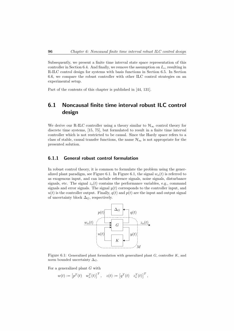
96 Chapter 6: Noncausal finite time interval robust ILC control design

Subsequently, we present a finite time interval state space representation of thiscontroller in Section 6.4. And finally, we remove the assumption on Lc, resulting inR-ILC control design for systems with basis functions in Section 6.5. In Section6.6, we compare the robust controller with other ILC control strategies on anexperimental setup.

Part of the contents of this chapter is published in [44, 131].

6.1 Noncausal finite time interval robust ILC controldesign

We derive our R-ILC controller using a theory similar to H∞ control theory fordiscrete time systems, [15, 75], but formulated to result in a finite time intervalcontroller which is not restricted to be causal. Since the Hardy space refers to aclass of stable, causal transfer functions, the name H∞ is not appropriate for thepresented solution.

6.1.1 General robust control formulation

In robust control theory, it is common to formulate the problem using the gener-alized plant paradigm, see Figure 6.1. In Figure 6.1, the signal wo(t) is referred toas exogenous input, and can include reference signals, noise signals, disturbancesignals, etc. The signal zo(t) contains the performance variables, e.g., commandsignals and error signals. The signal y(t) corresponds to the controller input, andu(t) is the controller output. Finally, q(t) and p(t) are the input and output signalof uncertainty block ∆G, respectively.

p(t) q(t)

u(t)

wo(t)

y(t)

zo(t)

∆G

G

K

M

Figure 6.1: Generalized plant formulation with generalized plant G, controller K, andnorm bounded uncertainty ∆G.

For a generalized plant G with

w(t) :=[pT (t) wT

o (t)]T

, z(t) :=[qT (t) zT

o (t)]T

,

6.1: Noncausal finite time interval robust ILC control design 97

the finite time interval robust control problem consists of finding a robust con-troller K which minimizes the induced 2-norm of the mapping M : w(t) 7→ z(t),subject to a worst case disturbance w(t), [15, 75]:

γopt = minu(t)

maxw(t)

‖M‖i2, t ∈ [0, N − 1]. (6.1)

Since the solution of (6.1) is in general difficult to obtain, see, e.g., [143], we focuson finding a solution to a sub-optimal robust control problem for γ > γopt. Forthat purpose, we require the following result.

Lemma 6.1. Given the optimization problem

maxx

1/2xT Qx + cT x, subject to Ax = b.

This optimization problem has a unique solution if A is of full rank and Q ≺ 0on the subspace ker(A), i.e., on the subspace x : Ax = 0.

Proof. See Section 10.3 and Section 14.1 in [80].

Based on Lemma 6.1, we can pose the finite interval sub-optimal robust controlproblem.

Proposition 6.1. Let (z, w, u, y) be the lifted representation of the finite timeinterval signals (z(t), w(t), u(t), y(t)) for t = 0, . . . , N−1. Furthermore, considerthe generalized plant[

zy

]=

[G11 G12

G21 0

] [wu

], (6.2)

and the finite interval sub-optimal robust control problem

minu

maxw

J , with (6.3)

J =1/2(G11w + G12u)T (G11w + G12u)− 1/2γ2wT w

+ λT (y −G21w),

where λ is a Lagrange multiplier.

Given γ, then there exists a solution for (6.3), i.e., a saddle point, if G12 hasfull column rank, G21 has full row rank, and GT

11G11 − γ2I ≺ 0 on the subspaceker(G21), i.e., on the subspace w : G21w = 0.

Proof. See Appendix A.6.1 for a sketch of the proof.


Note that existence of a unique solution for (6.3), i.e., the saddle point, does notnecessarily imply that ‖M‖i2 < γ. Optimization of γ such that ‖M‖i2 is smallerthan γ is left for Section 6.3.

Under the conditions of Proposition 6.1, the solution for (6.3) is obtained bydifferentiating J with respect to u, w, and λ, and setting the expressions equalto zero. The controller K then corresponds to the mapping K : y 7→ u.

Due to the definition of our robust control problem (6.1), the controller K clearlyoperates on a finite time span t ∈ [0, N − 1]. That this K is not restricted to becausal will become clear in the following section.

6.1.2 Noncausal finite time interval robust ILC control design

In the previous section, we have formulated the finite time interval robust controlproblem for an arbitrary generalized plant G. Here, we formulate a specific gen-eralized plant and solve (6.3) to find the finite time interval R-ILC controller.

To find the expression for the generalized plant, we define the variables (z, y, w, u)based on the following considerations:

• The desired control structure is given by (5.3).

• The main objective of our R-ILC control problem is to minimize the errorat trial k + 1, i.e., ek+1. With ek given by ek = yd − Jfk −Wipk, the errorek+1 can be given by

ek+1 = ek + J(fk − fk+1) + Wi(pk − pk+1). (6.4)

• ek+1 is a function of both pk and pk+1. As a result, in Figure 6.1 we consider∆G = diag(∆,∆) with inputs qk and qk+1.

• We want to include an additional objective to penalize the change of thecommand signal between two trials, i.e., f∆ = fk+1 − fk, using a weightingR1/2 with R = (R1/2)T R1/2.

Based on these considerations, (z, y, w, u) can be given by (6.5), and the general-ized plant G by (6.6). The resulting generalized plant formulation is presented inFigure 6.2.

z =[qTk qT

k+1 eTk+1 fT

∆

]T (6.5a)

y =[eTk fT

k

]T (6.5b)

w =[pT

k pTk+1 eT

k fTk

]T (6.5c)u = fk+1. (6.5d)

6.1: Noncausal finite time interval robust ILC control design 99

qk

qk+1

ek+1

f∆

ek

fk

=

0 0 0 Wo 00 0 0 0 Wo

Wi −Wi I J −J0 0 0 −R1/2 R1/2

0 0 I 0 00 0 0 I 0

︸︷︷︸

G

pk

pk+1

ek

fk

fk+1

. (6.6)

f∆

ek

ekfk

fk

qk+1pk+1

fk+1

pk qk

ek+1

G

Q, Lo

∆G

Figure 6.2: Generalized plant formulation for the R-ILC problem.

Using Lemma 6.1, in Corollary 6.1 we present existence conditions of a robustcontroller for the generalized plant (6.6).

Corollary 6.1. Given the robust control problem (6.3) for generalized plant (6.6).There exists a unique solution for (6.3), if R > 0 and γ >

√2σ(Wi).


Given the generalized plant and existence conditions, we solve (6.3) to find thefinite time interval R-ILC controller, see Proposition 6.2.

Proposition 6.2. Given (6.6) with its inputs and outputs defined by (6.5), R > 0and γ >

√2σ(Wi). Then the controller that solves (6.3) is given by

Q = (JT QJ + S + R)−1(JT QJ + R) (6.7a)

Lo = (JT QJ + S + R)−1JT Q, (6.7b)

with

Q = (I − 2γ−2WiWTi )−1 and S = WT

o Wo. (6.8)



Note that the existence condition γ >√

2σ(Wi) is also visible in the conditionQ 0.Remark 6.1. Since Q and Lo both are a function of the upper triangular blockToeplitz matrix JT , for this case the obtained ILC controller is noncausal.Remark 6.2. In the derivation of the R-ILC controller, we find that the worst casedisturbance satisfies pk+1 = −pk. With the trial periodicity of this disturbanceequal to ` = 2, it corresponds to the worst case trial varying disturbance foundin Section 4.5.

6.2 R-ILC analysis

In this section, the convergence and performance properties of R-ILC controlledsystem are studied. The obtained insight will subsequently be used in Section 6.3to optimize the R-ILC controller parameters.

Since the R-ILC controller of Proposition 6.2 fits the LQ norm optimal ILC controlsolution, the results from LQ norm optimal ILC (Section 5.6) are exploited in theanalysis. The difference between LQ norm optimal ILC and R-ILC lies in the factthat in LQ norm optimal ILC the weightings Q and S are user defined, while inR-ILC these weightings are the result of the specific robust problem formulation.

6.2.1 Convergence

As we already discussed in Section 5.6, monotonic convergence of R-ILC requiresJT QJ + S to be positive definite. With Wo a full rank matrix and Q > 0 for allpermissable γ, MC with R-ILC is always achieved.

Based on Corollaries 5.7 and 5.8, we know that RMC of the R-ILC controlleris achieved for sufficiently large S. We leave it for Section 6.3, to show how tooptimize the R-ILC controller such that RMC can be guaranteed for given modeluncertainty (Wi,Wo).

Finally, equal to LQ norm optimal ILC, the weighting R is the dominant factorfor convergence speed.

6.2.2 Performance

For performance, we focus on the asymptotic error e∞. With e∞ = yd − J∆f∞,and asymptotic command signal f∞ given by

f∞ = (Q− LoJ∆)f∞ + Loyd

= (I −Q+ LoJ∆)−1Loyd,

6.3: R-ILC parameter optimization 101

the asymptotic error equals

e∞ =(I − J∆ (I −Q+ LoJ∆)−1

Lo

)yd. (6.9)

Substitution of (6.7) in (6.9) subsequently yields

e∞ = (I − J∆(JT QJ∆ + S)−1JT Q)yd. (6.10)

From (6.10), we can see that R (still) does not influence e∞ of (6.10). In contrast,in Section 4.5, we showed that the influence of trial varying disturbances onperformance can be reduced by increasing R.

From Lemma 5.1, we know that the asymptotic error can be made smaller byreducing the gains in S relative to Q, i.e., reducing the penalty on fk+1 relativeto ek+1. For Q and S defined by (6.8), e∞ = 0 can not be achieved for all yd. Aswe will show in Section 6.3, though, freedom in the definition of (Wi,Wo) can beused to reduce ‖e∞‖2.

6.3 R-ILC parameter optimization

6.3.1 Optimizing over γ

The R-ILC controller from Proposition 6.2 has only one parameter γ. Optimizingthis R-ILC controller consists of finding an approximate for γopt, denoted by γmin,within a user defined bound ε > 0: γmin < γopt + ε, such that ‖M‖i2 < γmin.

To find γmin, we first need the expression for the mapping M : w 7→ z. Thismapping M is obtained by closing the loop between G and (Lo,Q), and equals

qk

qk+1

ek+1

f∆

=

0 0 0 Wo

0 0 WoLo WoQWi −Wi I − JLo J(I −Q)0 0 R1/2Lo R1/2(Q− I)

︸︷︷︸

M

pk

pk+1

ek

fk

. (6.11)

Using (6.11), γmin can be obtained using a bisection algorithm, see Algorithm1, [117, Section 9.3] and [131]. Initiation of this bisection algorithm requires thedefinition of an upper and lower bound on the possible values for γ (γ and γ,respectively). The upper bound γ must be chosen sufficiently large to ensurean initial solution to the algorithm, i.e., to ensure that initially ‖M‖i2 < γ. Thelower bound is defined by γ >

√2σ(Wi). Furthermore, ε > 0 is used as a tolerance

for the distance between γ and γ.

Note that, similar to H∞ feedback control, the minimum value for γmin doesnot have to result in robust monotonic convergence of the ILC controlled system.


This issue of RMC of the R-ILC controlled system can, however, be resolved, aswe show now.

6.3.2 Optimizing over γ and d

In this section, we introduce a second parameter in the controller: d. Optimizingthe R-ILC controller now consists of finding desired values for both γ and d.

Gain d in R-ILC is based on the equivalence of uncertainty models Wi∆Wo and(d−1Wi)∆(dWo), and originates from D-scaling, see Proposition 5.2. Conse-quently, optimization of the R-ILC controller through γ and d is comparableto the DK-iteration in µ-synthesis.

As a result of the introduction of d, the weighting matrices Q and S, (6.8), changeto

Q = (I − 2γ−2d−2WiWTi )−1, S = d2WT

o Wo.

This, in turn, can be rewritten to

Q = (d2I − 2γ−2WiWTi )−1, S = WT

o Wo, (6.12)

with γ >√

2d−1σ(Wi).

Optimizing the R-ILC control parameters deals with optimizing performance, i.e.,minimizing the asymptotic error e∞, while satisfying RMC conditions. Whilefrom Lemma 5.1 and (6.10), it can be concluded that performance improvementrequires an increase of Q relative to S, from Corollary 5.7 and Corollary 5.8,it can be concluded that RMC demands Q to be sufficiently small compared to

Algorithm 1 Bisection algorithm.Initiation: γ := γ, Ω := 1.while Ω = 1, do

Determine ‖M‖i2 for given γ, with M from (6.11).if ‖M‖i2 < γ holds, then

γ ← γelse

γ ← γend ifif γ − γ ≤ ε, then

γmin ← γΩ← 0

elseγ ← 0.5(γ + γ)

end if

end while

6.3: R-ILC parameter optimization 103

S. The goal of optimizing the R-ILC controller hence consists of manipulating γand d such that Q is maximized relative to S, while RMC of the ILC controlledsystem is guaranteed. This goal can be translated to: minimize d using, e.g.,a line search, subject to the constraint that the ILC controlled system is RMC.For each value of d, find γmin using Algorithm 1, with γ >

√2d−1σ(Wi). The

resulting d and γmin for which the ILC controlled system is just RMC, i.e., forwhich ‖D1/2

M MD−1/2M ‖i2 = 1−ε, with 0 < ε 1, constitutes the optimized R-ILC

controller.

The idea behind this optimization approach is to minimize the difference betweend2 and 2γ−2σ(Wi)2 to increase Q relative to S, while remaining RMC. Thereby,realize that the induced 2-norm of M is lower bounded by the induced 2-norm ofits elements, and hence that the difference between d2 and 2γ−2σ(Wi)2 is lowerbounded by the minimal value for γmin:

γmin > ‖M‖i2 ≥ max(√

2d−1σ(Wi), dσ(Wo)).

While the suggested optimization approach can be applied to all (Wi,Wo), for thespecial case (Wi,Wo) = (I,W ), optimization of γ and d can actually be simplifiedconsiderably, see Proposition 6.3.

Proposition 6.3. Consider the optimal R-ILC controller of Proposition 6.2 givenby (6.7), uncertainty (Wi,Wo) = (I,W ), and resulting control weightings Q = Iand S = dγWT W with dγ = d2−2γ−2 > 0. Then optimizing the R-ILC controllerwith respect to performance while remaining RMC is equivalent to minimizing dγ

while satisfying the RMC conditions.

The idea behind Proposition 6.3 is to minimize S relative to Q while remainingRMC, i.e., to optimize for performance under the constraint of RMC.

Once dγ is minimized, using, e.g., a bisection algorithm, there always exists γmin

and d for which ‖M‖i2 < γmin and dγ = d2 − 2γ−2min, namely

γmin = ‖M‖i2 + ε, d =√

dγ + 2γ−2min.

Note, however, that design of Lo and Q is a function of dγ only, and hence thatthere is no need to determine d and γmin explicitly.

6.3.3 Achievable performance as function of Wi and Wo

In general, there is a difference in achievable performance between the cases(Wi,Wo) = (W, I) and (Wi,Wo) = (I, W ). This can be explained by studyingthe influence of Wi and Wo on Q and S, respectively.

The case (Wi,Wo) = (I,W ) gives Q = I and S = dγWT W . For larger values forσ(W ) and dγ , we can find dγσ(W )2 > 1 (less error suppression in case of larger


model uncertainty), and for smaller values for σ(W ), we have gains in S ↓ 0 (nearfull error suppression in case of no model uncertainty).

The case (Wi,Wo) = (W, I) gives Q = (d2I − 2γ−2WWT )−1 and S = I. Whilefor larger values for σ(W ) and smaller values for d, we can find Q →∞ (near fullerror suppression in the presence of large model uncertainty), for smaller valuesfor σ(W ), we approach the lower bound Q ≈ d−2I (less error suppression in caseof no model uncertainty). Based on this reasoning, we can conclude that this caseconsiders the situation where the main disturbance in the ILC controlled systemis generated by Wi, instead of by yd.

Since ILC focusses on suppression of yd instead of error suppression due to modeluncertainty, the best performance is obtained with (Wi,Wo) = (I, W ). In Section6.6, this case will be discussed.

6.4 R-ILC design: State space solutions

The R-ILC solution of Proposition 6.2 can also be expressed in state space nota-tion. A huge benefit of this state space solution over the matrix solution, is thereduction in required buffer size to store the controller. Furthermore, the statespace solution does not have to be redesigned if the trial length changes, and thisformulation might simplify the inclusion of different uncertainty structures in theR-ILC control problem. Note, however, that inclusion of basis functions in thestate space solution is, in general, not straightforward, and that determination ofγmin can be difficult.

To find the state space solution for the R-ILC controller, we use the generalizedplant presented in Figure 6.1. The underlying structure of the generalized plantG is given by

G :

x(t + 1)

z(t)y(t)

=

A B1 B2

C1 D11 D12

C2 D21 D22

x(t)w(t)u(t)

. (6.13)

Without loss of generality, D22 can be set equal to zero, [81, 143]. Moreover,to guarantee the existence of a converging ILC controller, the generalized plant(6.13) is assumed to satisfy the following conditions, [117].

1. (C2, A) is detectable.

2. (A,B2) is stabilizable.

3. D12 has full column rank.

4. D21 has full row rank.

6.4: R-ILC design: State space solutions 105

5.[A− ejθ B1

]has full row rank ∀θ ∈ [0, 2π].

6.[A− ejθ

C1

]has full column rank ∀θ ∈ [0, 2π].

Note that conditions 5) and 6) are actually not required for finite time intervals.Nonetheless, throughout this section, we assume that the conditions 1) to 6) aresatisfied, and that a solution for the robust control problem exists.

6.4.1 General finite time interval robust solution

Although the following results are known from literature, e.g., [15, 24], we presenta summary of the results in a way suitable for ILC.

Based on Proposition 6.1, the robust optimization problem with G of (6.13) canbe given by

maxw(t)

minu(t)

N−1∑t=0

[1/2zT (t)z(t)− γ2

2wT (t)w(t)

], (6.14)

subject to

x(t + 1) = Ax(t) + B1w(t) + B2u(t)y(t) = C2x(t) + D21w(t).

By introducing the Lagrange multipliers λ(t) and λ2(t), the constraints in (6.14)can be incorporated in the cost function. Consequently, the constrained optimiza-tion problem (6.14) can be replaced by the unconstrained optimization problem

maxw(t)

minu(t)

J , (6.15)

with J =N−1∑t=0

[1/2zT (t)z(t)− γ2

2wT (t)w(t)

+ λT (t + 1)(−x(t + 1) + Ax(t) + B1w(t) + B2u(t))

+ λT2 (t + 1)(−y(t) + C2x(t) + D21w(t))

].

The solution for (6.15), i.e., the saddle point, is obtained by differentiating J withrespect to x(t), u(t), w(t), λ(t + 1), and λ2(t + 1), and setting the expressionsequal to zero. To simplify the result, we assume that C2 = 0. As we will show,this assumption holds for the generalized plant used in the design of the statespace R-ILC controller.


After some algebraic manipulations, see Appendix A.6.4, the solution is given by

[x(t + 1)

λ(t)

]=

[H11 H12

H21 HT11

] [x(t)

λ(t + 1)

]+

[F1

F2

]y(t)

u(t) =[G1 G2

] [x(t)

λ(t + 1)

]+ Hyy(t),[

x(0)λ(N)

]=

[x0

0

], (6.16)

with the elements in (6.16) equal to

H11 = A + B1E2DT11C1

− (B1E2DT11D12 + B2)E−1

3 (DT12C1 + DT

12D11E2DT11C1)

H12 = B1E2BT1 − (B1E2D

T11D12 + B2)E−1

3 (DT12D11E2B

T1 + BT

2 )

H21 = CT1 C1 + CT

1 D11E2DT11C1

− (CT1 D12 + CT

1 D11E2DT11D12)E−1

3 (DT12C1 + DT

12D11E2DT11C1)

F1 =(B1 − (B1E2D

T11D12 + B2)E−1

3 DT12D11

)E−1

1 DT21(D21E

−11 DT

21)−1

F2 =(CT

1 D11 − (CT1 D12 + CT

1 D11E2DT11D12)E−1

3 DT12D11

)E−1

1 DT21(D21E

−11 DT

21)−1

G1 = −E−13 (DT

12C1 + DT12D11E2D

T11C1)

G2 = −E−13 (DT

12D11E2BT1 + BT

2 )

Hy = −E−13 DT

12D11E−11 DT

21(D21E−11 DT

21)−1, (6.17)

and matrices E1, E2, and E3 defined as

E1 := (γ2I −DT11D11)−1

E2 := E−11 − E−1

1 DT21(D21E

−11 DT

12)−1D21E

−11

E3 := DT12D12 −DT

12D11E2DT11D12.

6.4.2 Finite time interval robust ILC

With the desire to express the R-ILC controller in state space notation, we usestate space models J and Wo = dW to construct the ILC controller. To simplifythe solution, we consider filter Wi = d−1I, d > 0. The gain d is a tuning gain,equal to the gain discussed in Section 6.3.


J :

xj(t + 1) = Ajxj(t) + Bjf(t)y(t) = Cjxj(t)

(6.18a)

Wo :

xw(t + 1) = Awxw(t) + Bwf(t)

q(t) = dC∗w︸︷︷︸Cw

xw(t) + dD∗w︸︷︷︸

Dw

f(t) (6.18b)

Wi : yw(t) = Wip(t). (6.18c)

Given (6.5), (6.13), and (6.18), we can formulate the generalized plant represent-ing our robust control problem with state x(t) given by

x(t) =

xkj (t)

xk+1j(t)

xkw(t)

xk+1w(t)

.

A closer look at the generalized plant, however, reveals that we can reduce itsorder. This follows from the fact that 1) the states xkj

(t) and xk+1j(t) are inde-

pendently driven by command signals fk(t) and fk+1(t), respectively,[xkj

(t + 1)xk+1j

(t + 1)

]=

[Aj 00 Aj

] [xkj

(t)xk+1j

(t)

]+

[Bj 00 Bj

] [fk(t)

fk+1(t)

],

and that 2) these states only appear in the performance output ek+1(t) as xk+1j(t)−

xkj(t)

ek+1(t) = ek(t)− Cj(xk+1j (t)− xkj (t))−Wi(pk+1(t)− pk(t)).

Hence, only the change of the states xj(t) from one trial to the next is of impor-tance for ILC.

By defining x(t) using state xkj (t) = xk+1j (t) − xkj (t) instead of xkj (t) andxk+1j

(t), we find the reduced order generalized plant with variables

x(t) =

xkj(t)

xkw(t)

xk+1w(t)

, w(t) =

pk(t)

pk+1(t)ek(t)fk(t)

, u(t) =[fk+1(t)

]

z(t) =

qk(t)

qk+1(t)ek+1(t)

fk+1(t)− fk(t)

, y(t) =[ek(t)fk(t)

],

(6.19)


with the different elements in the generalized plant of (6.16) given by

A =

Aj 0 00 Aw 00 0 Aw

, B1 =

0 0 0 −Bj

0 0 0 Bw

0 0 0 0

, B2 =

Bj

0Bw

C1 =

0 Cw 00 0 Cw

−Cj 0 00 0 0

, D11 =

0 0 0 Dw

0 0 0 0Wi −Wi I 00 0 0 −R1/2

C2 = 0, D11 =[0 0 I 00 0 0 I

], D12 =

0

Dw

0R1/2

, D22 = 0. (6.20)

Substitution of (6.20) in (6.17), see Appendix A.6.5, yields the desired finite timeinterval R-ILC controller (6.16), with elements[

H11 H12

H21 HT11

]=

[Ah −BhR−1

h BTh

CTh QhCh AT

h

](6.21)

Bh =

Bj

0Bw

, Sh =[0 0 (DT

wDw + R)−1DTw

]

Ch =

Cj 0 00 Cw 00 0 Cw

, Ah =

Aj 0 00 Aw 00 0 Aw

−BhShCh

R−1h = (DT

wDw + R)−1, Qh =

γ2

γ2−2W 2iI 0 0

0 I 00 0 (I + DwR−1DT

w)−1

,

and

F1 = BhR−1h

[0 R

]+

−I 0 00 0 I0 0 0

Bh

[0 I

], G1 = −ShCh

F2 = CTh Qh

−I 00 Dw

0 DwR−1h R

, G2 = −R−1h BT

h

Hy =[0 R−1

h R].

(6.22)

Finally, note that determination of a value for γmin of noncausal state space mod-els over a finite time interval is not always straightforward, due to the finiteness


of the state space representation of M . For relatively short trial spans, e.g., inour experience N < 500, we can find γmin by constructing M of (6.11), and usingthe bisection algorithm presented in Algorithm 1. For larger trial spans, however,the computational load of the lifted notation becomes too large. Although a fre-quency domain expression of M makes it possible to handle longer trial spans,expressing the controller in frequency domain and subsequently analyzing M(ejθ)only results in approximate results, see Lemma 5.2. How to find a value for γmin

for larger trial spans remains unanswered in this thesis.

6.4.3 Implementation of the finite time interval robust con-troller

Solution (6.16) is not implementable in its current form, since the causal andanti-causal dynamics are not separated. This implementation issue can, however,be resolved by performing a similarity transformation which separates the causalpart of the system from the anti-causal part, see [15, 90].

In this section, we discuss a time varying and time invariant similarity transforma-tion. Both transformed R-ILC controllers show the time domain behavior whichis hidden in the lifted R-ILC controller (Q, Lo). The benefit of the time varyingtransformation over the time invariant one is, that boundary conditions do notplay a role in the solution. A drawback is, that a larger buffer size is required tostore the time varying system matrices.

Conform the findings in Lemma 5.2, the time invariant transformation reveals thatan LTI representation of the finite time interval ILC controller includes nonzeroboundary conditions. Moreover, due to its LTI structure, the LTI solution can beused for a frequency domain interpretation of the obtained R-ILC controller.

Time varying similarity transformationAlthough different time varying similarity transformations are possible, we usethe time varying transformation discussed in [90]:[

g(t)λ(t)

]=

[I Y (t)0 I

] [x(t)λ(t)

]. (6.23)

Substitution of (6.23) in (6.16), see Appendix A.6.6, subsequently results in[g(t + 1)

λ(t)

]=

[AT1(t) 0AT2(t) (AT1(t))T

] [g(t)

λ(t + 1)

]+

[FT1(t)FT2(t)

]y(t),

u(t) =[G1 G2

] [g(t)

λ(t + 1)

]−G1Y (t)λ(t) + Hyy(t),[

g(0)λ(N)

]=

[x0 + Y (0)λ(0)

0

]=

[x0

0

], (6.24)


with the different matrices described by

AT1(t) = Ah(I + Y (t)CTh QhCh)−1

AT2(t) = (I + CTh QhChY (t))−1CT

h QhCh

FT1(t) = F1 −AhY (t)(I + CT

h QhChY (t))−1

F2

FT2(t) =(I + CT

h QhChY (t))−1

F2. (6.25)

The expression for Y (t) is obtained by setting the mapping λ(t + 1) 7→ g(t) equalto zero. As a result of this, we find the time varying Riccati equation

Y (t + 1) = AhY (t)(I + CTh QhChY (t))−1AT

h + BhR−1h BT

h

= AhY (t)ATh + BhR−1

h BTh

−AhY (t)CTh

(Q−1

h + ChY (t)CTh

)−1ChY (t)AT

h , (6.26)

with Y (0) = 0.

For implementation of (6.24), first determine Y (t) for t = 0, 1, . . . , N − 1 anduse Y (t) to determine (6.25). Next, calculate g(t + 1), followed by λ(t). Finally,determine u(t). Note that calculation of Y (t) and (6.25) has to be done onlyonce, before the first trial. The computational burden between trials is limited tocalculating g(t + 1), λ(t), and u(t).

Time invariant similarity transformationThe results presented here are based on the LQ norm optimal solutions presentedin [37, 39, 57]. An important difference between the results from [37, 39] and theones presented here, is that we obtain a (minimal order) state space solution forthe ILC controller as a whole, while in [37, 39] the state space solution consistsof the Hamiltonian system (6.16) together with an adjoint system.

The first step in finding an LTI implementable counterpart for (6.16) is similarto (6.23), but then with constant matrix Y[

g(t)λ(t)

]=

[I Y0 I

] [x(t)λ(t)

]. (6.27)

Unsurprisingly, this transformation results in time invariant (6.24) and (6.25) inwhich Y (t) is replaced by Y . The expression for Y is obtained by solving thediscrete algebraic Riccati equation (DARE)

Y = AhY ATh + BhR−1

h BTh −AhY CT

h

(Q−1

h + ChY CTh

)−1ChY AT

h , (6.28)

Note that solving this DARE requires Qh to be of full rank.

The second step is based on the similarity transformation[g(t)ζ(t)

]=

[I 0X I

] [g(t)λ(t)

]. (6.29)


After algebraic computations, see Appendix A.6.7, we find the decoupled LTIR-ILC controller[

g(t + 1)ζ(t)

]=

[AT1 00 AT

T1

] [g(t)

ζ(t + 1)

]+

[FT1

FT2 − (AT1)T XFT1

]y(t)

u(t) =[G1(I + Y X) −G2X

] [g(t)

g(t + 1)

]+

[−G1Y G2

] [ζ(t)

ζ(t + 1)

]+ Hyy(t), (6.30)

with X the solution to the Sylvester equation

A−TT1 X −XAT1 = −A−T

T1 AT2.

Although these LTI dynamics of (6.30) capture the time domain behavior of theR-ILC controller, we do not yet know the value of the boundary conditions forg(0) and ζ(N). We do, however, know that

g(N) = ANT1g(0) +

N−1∑j=0

AN−1−jT1 FT1y(j)︸︷︷︸

φg

ζ(0) = (ATT1)

Nζ(N) +N−1∑j=0

(ATT1)

N−1−j(FT2 −ATT1XFT1)y(N − 1− j)︸︷︷︸

φζ

.

Together with the overall similarity transformation[g(t)ζ(t)

]=

[I YX I + XY

] [x(t)λ(t)

]→

[x(t)λ(t)

]=

[I + Y X −Y−X I

] [g(t)ζ(t)

], (6.31)

we can find the relationx(0)λ(N)φg

φζ

=

I + Y X −Y 0 0

0 0 −X I−AN

T1 0 I 00 I 0 −(AT

T1)N

︸︷︷︸

Tbound

g(0)ζ(0)g(N)ζ(N)

g(0)ζ(0)g(N)ζ(N)

= T−1bound

x(0)λ(N)φg

φζ

. (6.32)

With the righthand side of (6.32) fully known, the boundary conditions g(0) andζ(N) can be calculated using (6.32).


Before implementing the LTI R-ILC controller, determine matrices Y and X, andthe values of the elements in (6.30) and T−1

bound. Between each trial, calculate theboundary values g(0) and ζ(N), see (6.32), and solve (6.30).

Remark 6.3. Instead of using a Riccati and Sylvester equation to decouple thecontroller dynamics, we can also use[

x(t)λ(t)

]=

[I −YX I

] [g(t)ζ(t)

][g(t)ζ(t)

]=

[(I + Y X)−1 (I + Y X)−1Y

−(I + XY )−1X (I + XY )−1

] [x(t)λ(t)

].

In this case, Y results from (6.28), and X from the DARE

X = ATh XAh −AT

h XBh(Rh + BTh XBh)−1BT

h XAh + CTh QhCh.

Finally, to make a frequency domain representation of the LTI controller possible,(6.30) is rewritten to[

g(t + 1)ζ(t + 1)

]=

[AT1 00 (A−1

T1)T

] [g(t)ζ(t)

]+

[FT1

−(A−1T1)T FT2 −XFT1

]y(t)

u(t) =[G1(I + Y X)−G2XAT1 G2(A−1

T1)T −G1Y] [

g(t)ζ(t)

]+

(−G2(A−1

T1)T FT2 + Hy

)y(t).

Although the boundary conditions are an essential part of the R-ILC controller,in a frequency domain representation, they are not taken into account. Conse-quently, the frequency domain R-ILC controller description can only be used fora frequency interpretation of the controller, not for implementation.

6.5 R-ILC design for uncertain systems with basisfunctions

Until now, we focussed on R-ILC for systems performing servo tasks. In thissection, we consider lifted R-ILC design for systems with basis functions. For thispurpose, we explicitly take into account the rank conditions of the system, result-ing in Lc 6= Ip. Design of Lc is, however, not considered here. For suggestions forLc, see Section 3.3.

The R-ILC design problem in this section is based on the uncertain system givenby H∆ and ILC framework presented in Figure 5.5. Due to the introduction ofbasis functions, the error objective in (6.5) changes from ek+1 to εk+1. Further-more, the input of the R-ILC controller is chosen as uk and εk, and the output asuk+1. Finally, the command signal fk+1 is given by fk+1 = Lim

c uk+1.

6.6: Example 113

The generalized plant G used to derive the R-ILC controller now equalsqk

qk+1

εk+1

fk+1 − fk

εk

uk

=

0 0 0 VoLc 00 0 0 0 VoLc

Vi −Vi In HLc −HLc

0 0 0 −R1/2Limc R1/2Lim

c

0 0 In 0 00 0 0 Ip 0

pk

pk+1

εk

uk

uk+1

. (6.33)

With the generalized plant defined, we use Proposition 6.2 to find the R-ILCcontroller:

Q = (LTc HT QHLc + S + LimT

c RLimc )−1(LT

c HT QHLc + LimT

c RLimc )

(6.34)

Lo = (LTc HT QHLc + S + LimT

c RLimc )−1LT

c HT Q, (6.35)

with

Q = (I − 2γ−2ViVTi )−1 and S = LT

c V To VoLc, (6.36)

and γ >√

2σ(Vi).

From Q and S in (6.36), we can see that for R-ILC design for systems with basisfunctions only model uncertainty Vi = TyWi and Vo = WoTf are relevant forR-ILC control design.

6.6 Example

In this section, the designed R-ILC controller is compared to LQ norm optimalILC and robust ILC control based on a frequency domain µ procedure, [34]. First,experimental result are presented. Second, the frequency domain interpretationof the LTI R-ILC controller of Section 6.4 is compared to that of µ ILC.

6.6.1 System description

The uncertain system used in this section represents a mass produced mechanicalSISO system showing production tolerances, see Figure 6.3 and Appendix C.

The frequency response of the nominal model J(z), upper bound for the uncer-tainty of this system W (z), and additive uncertainty data from measurements arepresented in Figure 6.4. Variations in experimental data are caused by the pro-duction tolerances. Since even the inverse model based ILC is RMC for relatively


Figure 6.3: Two-inertia setup used for the experiments.

small model uncertainty, see Corollary 5.9, no attempts have been made to accu-rately upper bound the model uncertainty corresponding to low frequent dynam-ics. Using the impulse responses of J(z) and W (z), N = 500 and Ts = 1 · 10−3s,we find the finite time interval representation J ∈ R500×500 (square and rankdeficient due to a nonzero relative degree), and W ∈ R500×500 (square and of fullrank).

100

101

102

−100

−80

−60

−40

−20

0

20

frequency [Hz]

Mag

nitu

de [d

B]

Nominal System JAdd. Uncertainty Bound WMeasured Add. uncertainty

Figure 6.4: Frequency domain representation of nominal system J(z), upper bound onthe uncertainty W (z), and additive uncertainty data from measurements.

6.6: Example 115

6.6.2 Experimental results

The reference signal yd ∈ R500 used for experimentation is presented in Figure 6.5.With this reference signal, the actuator in the feedback controlled system (withoutILC) is pushed to its limits, i.e., approaches the saturation level of ±2.5 volts.

0 0.1 0.2 0.3 0.4 0.50

10

20

30

time [s]

Ref

eren

ce [r

ad]

Figure 6.5: Reference signal used for experimentation.

In the experiments, the R-ILC controller (QR, LRo ) of (6.7) with weights (Q,S, R) =

(I, dγWT W, 0) is compared to an LQ norm optimal ILC controller (QLQ, LLQo )

with weights (Q,S, R) = (I, sI, 0), and a robust ILC controller (Qµ(z), Lµo (z)),

with Lµo (z) designed using infinite-interval µ design and Qµ(z) a zero phase low

pass filter, see [34]. Optimizing the R-ILC control parameters has resulted indγ = 525. For LQ norm optimal ILC, tuning has led to s = 0.85. In µ ILC, ro-bustness is obtained by tuning the cut-off frequency of Qµ(z). The largest foundcut-off frequency for which the system is RMC is 25 Hz.

Experiments are conducted on five different setups of the two-inertia system. InFigure 6.6, convergence of the different command signals is presented. Since inthis case u0 = 0 and yd 6= 0, monotonic convergence of the ILC controlled systemsequals ‖fk+1−f∞‖2 < ‖fk−f∞‖2. This is subsequently approximated by ‖fk+1−f21‖2 < ‖fk−f21‖2, since f∞ is not available in practice. In Figure 6.6, we can seethat the finite time interval ILC controllers converge to (near) zero, while the µILC controller remains to fluctuate. As we will show, this phenomenon is causedby oscillatory boundary effects in the command signal, due to the implementationof an infinite-interval solution over a finite interval.

The 2-norm of the initial errors and asymptotic errors are presented in Table 6.1.These values are obtained by first determining the 2-norm of the errors for each ofthe five setups, and subsequently averaging them. ‖e0‖2 is approximately equalfor R-ILC, LQ norm optimal ILC, and the µ ILC controller. Clearly, the 2-normof the asymptotic error corresponding to R-ILC is significantly smaller than thatof the other two control approaches.


0 5 10 15 200

5

10

15

20

trial

||fk−

f 21|| 2

R−ILCLQ ILCµ ILC

Figure 6.6: Convergence of the ILC controlled systems.

Table 6.1: 2-norms of the different asymptotic error signals.

2-norm ‖e0‖2 ‖eR21‖2 ‖eLQ

21 ‖2 ‖eµ21‖2

value 90.2 0.546 5.06 1.32

The time domain asymptotic command and error signals of the three ILC con-trolled system are presented in Figure 6.7 and Figure 6.8, respectively. FromFigure 6.7, we can state that the command signals of the R-ILC and µ ILC con-troller contain higher frequencies than that of LQ norm optimal ILC. As a result,R-ILC and µ ILC can remove more high frequent error components which sub-sequently leads to smaller errors, see Table 6.1 and Figure 6.8. An explanationfor this difference can be explained as follows. In LQ norm optimal ILC, the Qfilter has a low pass characteristic that cuts off all singular values smaller than acertain threshold. Because the uncertainty of our example is associated with largesingular values, the cut off value of the Q filter is relatively high. The Q filter ofthe R-ILC controller, however, cuts off singular values that are associated withsingular vectors that are uncertain, independent of the magnitude of the singularvalue itself. As a result, R-ILC only gives robustness at the cost of performancewhere it is required.

From Figure 6.7 we can furthermore see that the command signals in R-ILC andµ ILC are comparable during Tst ∈ [0.05, 0.45]s. Large transients (the boundaryeffects) in the command signals of µ ILC, however, result in errors which arelarger than those of R-ILC. With these variations in the command signal of µILC per setup comparable to those between the different setups, the transientsare the cause of the oscillatory convergence behavior of µ ILC in Figure 6.6. Anexplanation for this effect in µ ILC is found in the fact that the frequency domainµ ILC control solution is based on a time invariant behavior of the system whichis valid for all time, i.e., a behavior in which transients do not play a role. Since

6.6: Example 117

transients are in general not negligible for a finite time interval, the frequencydomain µ ILC controller only generates a command signal (approximately) equalto that of the R-ILC controller during that part of the trial where transients arenegligible. In this example, this time interval equals Tst ∈ [0.05, 0.45]s.

0 0.1 0.2 0.3 0.4 0.5−2

0

2

0 0.1 0.2 0.3 0.4 0.5−2

0

2

Com

man

d si

gnal

[V]

0 0.1 0.2 0.3 0.4 0.5−2

0

2

time [s]

Figure 6.7: Asymptotic command signals for R-ILC (top), LQ norm optimal ILC (cen-ter), and µ ILC (bottom).

6.6.3 Frequency domain controller interpretation

In Section 6.4, we derived a causal state space representation of the R-ILC con-troller. Here, we compare the frequency domain representation of this state spacemodel with the µ ILC controller to obtain insight in the frequency domain behav-ior of R-ILC.

fk+1(z) = QR(z)fk(z) + LR(z)ek(z)fk+1(z) = Qµ(z)fk(z) +Qµ(z)Lµ(z)ek(z),

The considered frequency domain convergence conditions are given by

|QR(ejθ)− LR(ejθ)J(ejθ)| < 1, |Qµ(ejθ)(1− Lµ(ejθ)J(ejθ))| < 1,

for θ ∈ [−π, π].

In Figure 6.9, the Bode plots of LR(z) and Qµ(z)Lµ(z) are shown, together withthe inverse of model J(z). When focussing on the magnitude plot, we can see


0 0.1 0.2 0.3 0.4 0.5−0.5

0

0.5

0 0.1 0.2 0.3 0.4 0.5−0.5

0

0.5

Err

or e

21 [r

ad]

0 0.1 0.2 0.3 0.4 0.5−0.5

0

0.5

time [s]

Figure 6.8: Asymptotic error signals for R-ILC (top), LQ norm optimal ILC (center),and µ ILC (bottom).

that the µ ILC controller approximates J−1(z) up to 23 Hz. Consequently, µILC equals an inverse model based ILC controller up to 23 Hz. Moreover, thesignificant high frequent roll-off of Qµ(z)Lµ(z) can be explained by the high orderof the user designedQµ(z) low-pass filter. Contrary toQµ(z)Lµ(z), LR(z) alreadystarts to deviate from J−1(z) above 13 Hz. This deviation, however, remainsrelatively small up to 60 Hz.

When focussing on the phase plot, we see that the phase of LR(z) matches thephase of J−1(z) exactly. With the µ ILC controller designed to match J−1(z) upto a cut-off frequency of 25 Hz, the phase of Qµ(z)Lµ(z) only equals the phaseof J−1(z) up to 25 Hz. The high frequent phase lag is subsequently explained bythe fact that Lµ(z) is causal and Qµ(z) is designed to be zero phase.

Filters QR(z), Qµ(z), and W (z) are depicted in Figure 6.10. The Bode plot ofQµ(z) can be fully explained by the fact that Qµ(z) is user designed zero phaselow-pass filter. The explanation of QR(z) is more involved. The zero phasecharacteristic of QR(z) is most likely the result of the R-ILC objective regardingthe minimization of the error: With QR(z) = I for optimal performance, Lemma5.1, minimizing ‖I−QR(z)‖i2 for each frequency results inQR(z) being zero phase.Furthermore, we can see that QR(z) has a magnitude of approximately 1 forfrequencies smaller than 40 Hz and larger than 70 Hz. The low frequent gain canbe explained by the relatively small amount of model uncertainty in comparisonto J(z), see Corollary 5.9. The explanation for the high frequent properties ofQR(z) is found in the fact that the magnitude of the product LR(z)J∆(z) ≈ 0.

6.6: Example 119

100

101

102

−200−100

0100

Mag

nitu

de [d

B]

100

101

102

−202468

Frequency [Hz]

Pha

se [r

ad]

LR(z)

Qµ(z)Lµ (z)

J−1(z)

Figure 6.9: Bode plots of LR(z), Qµ(z)Lµ(z), and J−1(z).

As a result, QR(z) = 1 − ε with 0 < ε 1 is sufficient to obtain convergence.The only frequencies with |QR(z)| < 1 lie in the frequency band where both thecontrol gain LR(z) and the uncertainty W (z) is relatively large. Note that theseresults of QR(z) give a new perspective on the design considerations of the Q(z)filter.

100

101

102

−100

−50

0

Mag

nitu

de [d

B]

100

101

102

−6−4−2

02

Frequency [Hz]

Pha

se [r

ad]

QR(z)

Qµ (z)W(z)

Figure 6.10: Bode plots of QR(z), Qµ(z), and W (z).

The convergence conditions are presented in Figure 6.11. The nonzero magnitudesup to approximately 15 Hz can be explained by the small mismatches between thegains in (LR(z), Lµ(z)) and J−1(z). Moreover, the high frequent roll-off of the


µ condition can be explained by the characteristics of Qµ(z). The high frequentmagnitude 1 − ε for R-ILC can be explained by the fact that for these frequen-cies LR(z)J∆(z) is approximately zero, and hence that the convergence conditionequals QR(z). Finally, the R-ILC convergence condition shows a dip between40 Hz and 70 Hz to compensate for the relatively large uncertainty bound onLR(z)J∆(z).

100

101

102

−100

−50

0

Frequency [Hz]

Con

verg

ence

con

ditio

n

R−ILCµ ILC

Figure 6.11: Convergence condition for R-ILC and µ ILC.

We conclude the comparison between R-ILC and µ ILC with a discussion onachievable performance with both controllers. For that, we study the mappingfrom reference signal yd to asymptotic error e∞, see (6.9) and Figure 6.12. FromFigure 6.12, we can state that µ ILC can achieve a higher suppression of lowfrequent reference signals than R-ILC. On the other hand, above the cut-off fre-quency of 25 Hz, µ ILC does not improve performance at all (the gain equals1). In contrast, the R-ILC controller can improve performance up to roughly 200Hz, due to the specific characteristics of the QR(z) filter. Only in the frequencyband of 40-70 Hz performance improvement by R-ILC is very limited, due to therelatively large uncertainty bound.


In this chapter, we have presented a robust ILC control strategy that is robustagainst model uncertainty as given by an additive uncertainty model. The designmethodology has been based on H∞ optimization, however, modified such thatthe obtained ILC controller is not restricted to be causal and inherently operateson a finite time interval. We have analyzed the convergence and performanceproperties of resulting ILC controlled system, and provided guidelines to achieveoptimized performance while remaining robustly monotonically convergent. Tocircumvent the use of large dimensional system matrices in R-ILC, a state spacerepresentation for the R-ILC controller has been derived and implementation


100

101

102

−150

−100

−50

0

Frequency [Hz]

map

ping

from

yd to

e∞

R−ILC(z)µ ILC(z)

Figure 6.12: Amplitude mapping from reference signal yd to asymptotic error e∞ forR-ILC and µ ILC.

issues discussed. Finally, the R-ILC controller has been modified such that itis capable of handling systems with basis functions.

In an example, we have shown that the presented robust ILC control strategy hasbeen able to outperform LQ norm optimal ILC control and robust ILC controlbased on a frequency domain µ procedure. Moreover, in a comparison betweenµ ILC and a frequency domain interpretation of the R-ILC controller, we haveshown that the R-ILC clearly differs from µ ILC in phase characteristics of ILCcontrol element L(z), and magnitude characteristics in robustness filter Q(z).

123

Chapter 7

Conclusions andRecommendations

In this final chapter, the main results are recapitulated, and recommen-dations for further research presented.

7.1 Conclusions

We discuss the results of each research objective separately.

Objective 1The first research objective dealt with exploration of the design issues in ILC fortime-windowed systems (Chapter 3). With ILC for residual vibration suppres-sion in point-to-point motion problems largely unexplored, we have used this ILCtask as an exemplary case to analyze ILC for time-windowed systems. We havediscussed the several steps taken from formulation of the residual vibration sup-pression problem, via system representation with time windows, and ILC controldesign, to implementation of this problem on a SISO and MIMO flexible motionsystem. Thereby, we have introduced a novel ILC control framework suitable forILC for residual vibration suppression, and proven that there is the additionalfreedom in ILC control design for point-to-point motion problems related to ma-nipulation of the amplitude of the command signal.

Objective 2The second research objective focussed on the formulation of a unifying ILC frame-work, in which time-windowed systems and other ILC problem formulations are

124 Chapter 7: Conclusions and Recommendations

enclosed (Chapter 4). Furthermore, the properties of this unified framework wereto be studied. To meet the objective, first we have illustrated that various dif-ferent ILC formulations in the literature can be captured by a common systemrepresentation involving i/o basis functions. Analysis of ILC for this system rep-resentation has revealed how different ILC objectives can be reached by design ofseparate parts of the ILC controller. Moreover, we have used these results to sys-tematically design ILC controllers for the representation under study, and showedthat the obtained results are applicable to existing ILC problem formulations withi/o basis functions, and problem formulations which can be interpreted as such.

Objective 3The third objective was to develop an approach with which the robust conver-gence properties of existing finite time interval ILC controlled systems with modeluncertainty can be analyzed (Chapter 5). For that purpose, a novel (MIMO) un-certain model representation over a finite time interval has been derived. Thisuncertainty representation, together with results from well developed µ analy-sis, has lead to the desired approach. Since the approach does not require theILC controller to obey specific properties, it is applicable to any trial invariantLTI/LTV, (non)causal, non(square) ILC control strategy. As an example, theobtained result has been applied to LQ norm optimal ILC, yielding new insightin the tuning guidelines for LQ norm optimal ILC.

Objective 4The fourth, and final, objective focussed on the design of a robust ILC controlstrategy which exploits knowledge about model uncertainty in its design, is notrestricted to behave causal, and incorporates the finite time interval aspect of ILC(Chapter 6). The robust ILC design methodology which we have derived to meetthis objective hinges on H∞ optimization, but modified such that the obtainedILC controller is not restricted to be causal and explicitly operates on a finite timeinterval. Analysis of the ILC controlled system with robust ILC controller hasrevealed how to optimize the controller parameters so as to optimize performancewhile remaining robustly monotonically convergent. In experiments, we haveillustrated that the designed robust ILC controller can outperform existing LQnorm optimal ILC controllers and causal µ based ILC controllers. Moreover, acomparison between the frequency domain interpretation of µ ILC (causal) andour proposed robust ILC (noncausal) has revealed differences in filter propertieswhich, until now, have been unknown in ILC literature.

This thesis has extended existing ILC results on the following issues:

• Illustration of the use of time windows in ILC by analyzing ILC for residualvibration suppression in point-to-point motion problems (Chapter 3)

• ILC control design for time-windowed systems (Chapter 3, Section 3.3)

• Proof and demonstration of new design freedom in ILC concerning manip-ulation of the command signal form (Chapter 3 Section 3.3, and Chapter 4Section 4.4)

7.2: Recommendations 125

• Introduction of a unifying ILC framework for linear systems with basis func-tions (Chapter 4, Section 4.2)

• Analysis and ILC control design for systems with basis functions in a uni-fying ILC framework (Chapter 4, Sections 4.3 to 4.5)

• Introduction of a novel uncertainty model representation over a finite timeinterval (Chapter 5, Section 5.1)

• Development of a robust monotonic convergence analysis approach for ex-isting finite time interval ILC controllers (Chapter 5, Sections 5.3 and 5.4)

• Proof that a frequency domain monotonic convergence analysis provides asufficient condition for finite time interval if the ILC controllers is causal.Illustration that for noncausal ILC controllers this does not necessarily hold(Chapter 5, Section 5.3)

• Analysis of the robustness properties of LQ norm optimal ILC controllers(Chapter 5, Section 5.5)

• Design and optimization of a noncausal finite time interval robust ILC con-troller (Chapter 6, Sections 6.1 to 6.5)

• The proof that finite time interval linear time invariant ILC control solutionsrequire nonzero initial conditions (Chapter 6, Section 6.4)

7.2 Recommendations

The results of this thesis have given rise to suggestions for further research.

System identification for ILCWe showed that, even without additional robustness filters, ILC controllers arerobustly monotonically convergent for relatively small amounts of model uncer-tainty. Consequently, we can achieve optimal performance in case of little uncer-tainty. Based on our findings, we expect that optimal performance can be reachedif the true system can be captured by a nominal model with an uncertainty setwith bounds which are smaller than 100% of the nominal model. The remainingquestions are:

• Should system identification for ILC focus on reduction of the uncertaintyset to maximally 100% of the nominal model?

• Do other issues play a role in system identification for ILC (or in systemidentification for feedforward control in general)?

126 Chapter 7: Conclusions and Recommendations

Trial varying uncertaintyFor a system that is subject to wear, the dynamics can change during its lifespan.As a result, an ILC controlled system which is convergent in the first part ofoperation, might become unstable later on. In our discussion on robust conver-gence conditions and robust ILC control design, we have not taken this issue intoaccount. Inclusion of this type of model uncertainty in ILC analysis and designgives rise to the following questions:

• How do we capture trial varying model uncertainty, while respecting thefinite time aspect of a trial?

• Can we modify the existing robust monotonic convergence conditions (Chap-ter 5) to accommodate for trial varying model uncertainty? A positiveanswer to this question might be found by first writing the trial varyinguncertainty model as a trial domain state space model, and second, usingthe M∆M structure of Chapter 5 to find the robust convergence conditions.In this case, we expect ∆M to be equal to ∆M = diag(∆,∆P , δI).

• Given a model of the trial varying disturbance, can we use the design ap-proach of Chapter 6 to find the robustly monotonically converging ILCcontroller with optimized performance? Or can we combine the design ap-proach of Chapter 6 with robust ILC control design of [89], to find thedesired controller?

Robust monotonic convergence conditionsThe robust monotonic convergence (RMC) conditions for LTI and LTV uncer-tainty models derived in this thesis (Chapter 5) are sufficient. Further researchcan focus deriving less conservative RMC results.

Optimization of state space robust ILC for relatively long trial spansTo avoid large dimensional system matrix representations and to be more flexi-ble to changes in trial length, we introduced a state space representation of therobust controller (Chapter 6). Although we solved the design and implementa-tion issues, it remains an open question how to properly optimize the controllerparameters such that performance is optimized in presence of robust convergence.

Experimental validationThe main purpose of the experimental results in this thesis is to demonstratefeasibility of the proposed concepts. A next step is to implement Hankel ILC androbust ILC on industrial applications.

127

Appendix A

Proofs and Derivations

A.2 Chapter 2

A.2.1 Proof Lemma 2.1

With fk+1 = (INqi− LJ)fk, MC requires

‖fk+1‖2 < ‖fk‖2‖(INqi

− LJ)fk‖2 < ‖fk‖2fT

k (INqi − LJ)T (INqi − LJ)fk < fTk fk.

For this inequality to hold for all f0, MC requires

λi((INqi− LJ)T (INqi

− LJ)− INqi) < 0 ∀i ∈ [1, Nqi]

⇔ ‖INqi− LJ‖i2 < 1.


Given J ∈ RNqo×Nqi , (2.8), and rank(LJ) = Nqi due to convergence. Thenfor k → ∞, the state fk = fk+1 = f∞ equals f∞ = (LJ)−1Lyd. As a result,e∞ = yd − Jf∞ is given by

e∞ =(INqo

− J(LJ)−1L)yd.

128 Appendix A: Proofs and Derivations

e∞ = 0 ∀yd implies INqo − J(LJ)−1L = 0. Using

rank

([A11 00 A22 −A21A

−111 A12

])= rank

([A11 A12

A21 A22

]),

e∞ = 0 ∀yd iff

rank([

LJ LJ INqo

])= Nqi ⇔ rank

([0 0J INqo

])= Nqi.

which holds iff qo = qi.

A.3 Chapter 3


Consider Lo ∈ Rp×nqo , Lc ∈ Rmqi×p, and LoJHLc ∈ Rp×p. Then convergencerequires ρ(Ip − LoJHLc) = maxj |1− λj(LoJHLc)| < 1 with j ∈ [1, p].

Only if: Consider the case p > rank(JH). Then rank(LoJHLc) < p indepen-dent of the choice for (Lo, Lc). Consequently, there exists j ∈ [1, p] for whichλj(LoJHLc) = 0 ⇒ ρ(Ip − LoJHLc) ≥ 1.

If: Consider p ≤ rank(JH). Then there exists (Lo, Lc) for which ρ(Ip−LoJHLc) <1. For example, Lo = gJ†o with g ∈ (0, 2) and Lc = J†c = JT

c (JcJTc )−1 yields

ρ(Ip − gIp) = |1− g| < 1.

With ρ(Ip−LoJHLc) < 1 implying rank(LoJHLc) = p, and with rank(LoJHLc) ≤min(rank(Lo), rank(JH), rank(Lc)), convergence requires rank(Lo) = rank(Lc) =p.


Given Lo, then pole placement in system (3.10) is possible by Lc, iff (Ip, LoJH)is controllable. (Ip, LoJH) controllable ⇔ rank(LoJH) = p. Using rank(LoJH) =rank(LoJoJc) ≤ min(rank(LoJo), rank(Jc)) = min(rank(LoJo), p), thenrank(LoJH) = p implies rank(LoJo) = p. Conversely, if LoJo ∈ Rp×p is nonsingu-lar, i.e., rank(LoJo) = p, then rank(LoJo) = p and rank(Jc) = p together implyrank(LoJH) = p.

Similarly, given Lc, then pole placement in system (3.10) is possible by Lo,iff (JHLc, Ip) is observable. (JHLc, Ip) observable ⇔ rank(JHLc) = p ⇔rank(JcLc) = p.

Appendix A: Proofs and Derivations 129


With (3.12) from Proposition 3.1, the trial domain dynamics are given by

uk+1 = (Ip − LoJo)uk + Loαd (A.1)

βk = J†c uk + T †c Mcuk, (A.2)

Furthermore, the asymptotic error ε∞ follows from

u∞ = (Ip − LoJHLc)u∞ + Loαd

= (LoJo)−1Loαd. (A.3)ε∞ = αd − JHLcu∞

= (Inqo− Jo(LoJo)−1Lo)αd, (A.4)

since JcT†c = 0. Then for arbitrary Mc ∈ R(mqi−p)×p, convergence of Hankel

ILC is defined by ρ(Ip − LoJo) < 1, (A.1), and performance by ‖ε∞‖2, with ε∞from (A.4). Additionally, every command signal βk which can be obtained from(A.1)-(A.4) by arbitrary Lo, can be reached by design of Mc.

A.3.4 Proof Proposition 3.2

Controller Lo : (εk, uk) 7→ uk+1 is obtained by minimizing

minuk+1

J , with

J = εTk+1εk+1 + (βk+1 − βk)T R(βk+1 − βk).

Using αd = εk + JHLcuk = εk + Jouk, we find εk+1 = εk − Jo(uk+1 − uk).Additionally, with βk = Lcuk, the optimization problem can be reformulated as

minuk+1

J , with

J = (εk − Jo(uk+1 − uk))T (εk − Jo(uk+1 − uk))

+ (uk+1 − uk)T LTc RLc(uk+1 − uk).

Solving this problem gives∂J

∂uk+1= 0 → uk+1 = uk + (JT

o Jo + LTc RLc)−1JT

o︸︷︷︸Lo

εk. (3.14∗)


Using (3.19), the optimization problem is given by

minMc

J = minMc

βT∞Wββ∞

=((LoJo)−1Loαd

)TLT

c WβLc

((LoJo)−1Loαd

).


Given Lc from (3.12) and γm := (LoJo)−1Loαd, J can be rewritten to

J = γTm(J†c + T †c Mc)T Wβ(J†c + T †c Mc)γm. (A.5)

The minimum of J is obtained by differentiating J with respect to Mc andrequiring it to be zero ∀γm. This results in T †

T

c WβT †c Mc = −T †T

c WβJ†c . WithT †c = TT

c (TcTTc )−1, Mc equals Mc = −TcT

Tc (TcWβTT

c )−1TcWβJ†c , which yieldsLc = (Imqi

− TTc (TcWβTT

c )−1TcWβ)J†c .

A.3.6 Singular value decomposition of JH

JH = UΣV T =[U1 U2

] [Σ1 00 0

] [V T

1

V T2

]= U1Σ1V

T1 , (A.6)

with JH ∈ Rnqo×mqi , U1 ∈ Rnqo×p, Σ1 ∈ Rp×p, V1 ∈ Rmqi×p,and Jo := U1Σ1, Jc := V T

1 , T †c = V2.

A.4 Chapter 4


Convergence: Follows from standard linear control theory.MC: Consider transformation zk = T−1uk with T such that TT LimT

c Limc T = Ip.

Then with zk+1 = T−1(Ip − LoHLc)Tzk and fk = Limc Tzk, ‖fk+1‖2 < ‖fk‖2

equals

‖Limc (Ip − LoHLc)Tzk‖2 < ‖Lim

c Tzk‖2 ⇔

zTk TT (Ip − LoHLc)T LimT

c Limc (Ip − LoHLc)Tzk < zT

k TT LimT

c Limc Tzk.

For this inequality to hold for all z0 ∈ Rp, MC requires

λi(TT (Ip − LoHLc)T LimT

c Limc (Ip − LoHLc)T − TT LimT

c Limc T ) < 0, (A.7)

∀i ∈ [1, p]. With TT LimT

c Limc T = Ip, this equals

λi

(TT (Ip − LoHLc)T (T−1)T T−1(Ip − LoHLc)T − I

)<0

⇔ ‖T−1(Ip − LoHLc)T‖i2 <1.



1) Using (4.7), (4.8), u∞ = (LoHLc)−1Loαd, ε∞ = αd − HLcu∞, and the rankcondition from Lemma 3.2, we find

ε∞ = (Ip −HLc(LoHLc)−1Lo)αd

= (Ip −HSc(SoPoHSc)−1SoPo)αd

= (Ip −Ho(PoHo)−1Po)αd.

2) From Corollary 4.1, we know that optimal performance is achieved for (Lo, Lc) :HcLc(LoHLc)−1Lo = H†

o ⇒ Po : (PoHo)−1Po = H†o. One possible solution

for Po is given by Po = HTo .


Given covariances (4.12) and (4.13), (4.7) with So = g(PoHo)−1 and g ∈ (0, 2),and (4.8) with Sc = Ip. Then Ruu equals

Ruu = (1− g)2Ruu + g2(PoHo)−1PoRddPTo (PoHo)−1T

=g

2− g(PoHo)−1PoRddP

To (PoHo)−1T

,

and Rεε is given by Rεε = Rdd + g2−g Ho(PoHo)−1PoRddP

To (PoHo)−1T

HTo . The

results for g = 0+, 1, 2− follow directly from Rεε.


Given Given (4.7) with So = g(PoHo)−1 and g ∈ (0, 2), and (4.8) with Sc = Ip.Then (4.14) equals

εask = ε∞ − (In −

g

w − 1 + gHo(PoHo)−1Po)dk(`).

The results for g = 0+, 1, 2− are obtained by analyzing εask for trial periodic

disturbance dk(` →∞) (w = ej2π/` → 1), i.e., almost trial invariant dk, and dk(2)(w = ej2π/` = −1), i.e., for disturbances dk+1 = −dk.


A.5 Chapter 5


Given the system in Figure 5.3. Then the mapping of the trial state zk 7→ zk+1

is given by

zk+1 = T−1(Q− Lo(J + Wi∆Wo)Lc)Tzk

= T−1(Q− LoJ∆Lc)Tzk,

and zk = ∆P zk+1. RC of the system in Figure 5.3 requires ρ(T−1(Q−LoJ∆Lc)T )< 1 ∀J∆ ∈ Π, which is equivalent to RC of (5.4) for the choice T = Ip. Thereplacement w−1Ip in Figure 5.2 by ∆P ∈ ∆P = δP Ip : δp ∈ C, |δP | < 1 inFigure 5.3 is suggested and proven in Section 4.2 in [103].

RMC of the system in Figure 5.3 in zk requires ‖T−1(Q−LoJ∆Lc)T‖i2 < 1 ∀J∆ ∈Π. This RMC condition is equivalent to that of (5.4) for T satisfying TT LT

c LcT =Ip. Furthermore, with the RMC condition in Lemma 5.1 equivalent to a robustperformance condition in robust feedback control, as discussed in, e.g., Section8.4 in [117], ∆P in Figure 5.3 is defined as ∆P ∈ ∆P ∈ Cp×p, ‖∆P ‖i2 < 1.


Consider J∆ and (Q, Lo) the finite dimensional (block) Toeplitz matrices repre-senting J∆(z) and (possibly noncausal) (Q(z), Lo(z)) over a finite time intervalof length N . Furthermore, consider (LJ)N the finite time interval representationof the product (Lo(z)J∆(z)).

From Proposition 2.3 in [19], we find that

LoJ∆ = (LJ)N − C,

with C containing truncation and Hankel operators. C = 0 iff both Lo and J∆ arelower triangular (block) Toeplitz matrices. Moreover, for A(z) with correspondingfinite dimensional (block) Toeplitz matrix AN , limN→∞ ‖AN‖i2 = ‖A(ejθ)‖i2, and‖AN‖i2 ≤ ‖A(ejθ)‖i2, see e.g., Section 1.3 and Section 6.4 of [20].

Now, Corollary 5.1 states that the ILC controlled system is RMC if ‖Q−LoJ∆‖i2 <1. Take Lo(z) causal, then Lo is an lower triangular (block) Toeplitz matrix,LoJ∆ = (LJ)N , Q− LoJ∆ is Toeplitz, and‖Q − LoJ∆‖i2 ≤ ‖Q(ejθ)− Lo(ejθ)J∆(ejθ)‖i2.


A.5.3 Proof Corollary 5.2

Given (5.9) withQ = LoJLc, and µ∆M(M) ≤ ‖D1/2

M MD−1/2M ‖i2. Then µ∆M

(M) <1 if

µ∆M(M) ≤ inf

d‖

[0 dWoLcT

−d−1T−1LoWi 0

]‖i2 < 1

⇒ mind

max(d‖WoLcT‖i2, d−1‖T−1LoWi‖i2) < 1.

Solving this for d gives

d = ‖T−1LoWi‖1/2i2 · ‖WoLcT‖−1/2

i2

µ∆M(M) ≤ ‖T−1LoWi‖1/2

i2 · ‖WoLcT‖1/2i2 .

As a result, ‖T−1LoWi‖i2 · ‖WoLcT‖i2 < 1 ⇒ µ∆M(M) < 1.


Consider (5.10), Q = LoJLc, and the fact that the inequality in (5.8) holds forLTI ∆. Furthermore, let Wo be given by (5.12). Thenµ∆M

(M) ≤ infD1/2 max(‖D1/2WoLcT‖i2, ‖T−1LoWiD−1/2‖i2), with D1/2 having

a structure equal to (5.10).

For D1/2 := dW−1o we find µ∆M

(M) ≤ mind max(d‖LcT‖i2, d−1‖T−1LoW‖i2),

with W := WiWo. Solving this for d gives µ∆M(M) ≤ ‖LcT‖1/2

i2 · ‖T−1LoW‖1/2i2 .

Since ‖LcT‖i2 = 1 by design of T , ‖T−1LoW‖i2 < 1 ⇒ µ∆M(M) < 1.


Given interval uncertainty as defined in Table 5.1 with ‖∆t‖i2 ≤ 1∀t ∈ [0, N − 1].Then following Section 7 in [45], the interconnection matrices T1 ∈ RNq×qN(N+1)/2

and T2 ∈ RqN(N+1)/2×Nq such that ∆ = T1∆∗T2 are given by

T1 =[INq

0q×q(N−1) · · · 0q(N−1)×q

Iq(N−1) · · · Iq

], (A.8)

T2 =[INq

Iq(N−1) · · · Iq

0q×q(N−1) · · · 0q(N−1)×q

]T

. (A.9)

Moreover, the block diagonal ∆∗ is norm bounded by 1, i.e., ‖∆∗‖i2 ≤ 1. Knowingthat det(I −M∆) = det(I −MT1∆∗T2) = det(I −T2MT1∆∗) = det(I −M∗∆∗),we find µ∆M

(M) with ∆M equal to µ∆M(M∗) with ∆∗

M . Consequently, we haveµ∆M

(M) ≤ ‖D∗1/2

M M∗D∗−1/2

M ‖i2, with

D∗M = diag(d0INq, d1Iq(N−1), . . . , dNIq, Ip) : dt > 0


commuting with ∆∗M = diag(∆∗,∆P ), see Section 7 of [45]. Finally, the upper

bound can be formulated as the LMI of (5.15), see Theorem 3.9 of [103]. Thiscondition is sufficient, since inequality in (5.8) holds for ∆ LTI, see Table 1 in[103].


Assume (5.24) RMC for r = 0. Then Corollary 5.1 states that there exists α suchthat

‖(JT QJ + S)−1JT QWi∆Wo‖i2 ≤ α < 1 ∀∆ ∈ ∆.

Due to the properties of (Q,S), JT QJ + S is symmetric positive definite. Con-sequently, its singular value decomposition equals JT QJ + S = UΣUT , with U aunitary matrix and Σ = diag(σi), i = 1, . . . , Nqi, of full rank.

RMC for R = rI > 0 subsequently requires

max∆∈∆

‖(JT QJ + S + rI)−1(rI − JT QWi∆Wo)‖i2

= max∆∈∆

‖(JT QJ + S + rI)−1(rI + JT QWi∆Wo)‖i2

= max∆∈∆

‖(JT QJ + S + rI)−1·

(rI + (JT QJ + S)(JT QJ + S)−1JT QWi∆Wo)‖i2

≤ ‖(JT QJ + S + rI)−1(rI + (JT QJ + S)α)‖i2

= ‖(UΣUT + rI)−1(rI + αUΣUT )‖i2

= ‖U(Σ + rI)−1(rI + αΣ)UT ‖i2

= ‖(Σ + rI)−1(rI + αΣ)‖i2

= maxi

(ασi + r

σi + r

)< 1 ∀r ≥ 0.

A.6 Chapter 6

A.6.1 Sketch of Proof Proposition 6.1

For given γ > γopt and t = 0, . . . , N − 1, the sub-optimal finite interval robustcontrol objective ‖M‖i2 < γ can be reformulated as


‖M‖i2 = supw,‖w‖>0

‖z(t)‖2‖w(t)‖2

< γ →

J c = 1/2‖z(t)‖22 − 1/2γ2‖w(t)‖22 < 0, t ∈ [0, N − 1].

The objective Jc can be used as an objective function for the robust controlsynthesis problem: Find a controller K : y 7→ u such that

minu(t)

maxw(t)

J c = minu(t)

maxw(t)

1/2N−1∑t=0

zT (t)z(t)− γ2wT (t)w(t),

is achieved, subject to the generalized plant relations.

Let (z, w, u, y) be the lifted representation of the finite time interval signals(z(t), w(t), u(t), y(t)) for t = 0, . . . , N − 1. Then the sub-optimal robust controlproblem is given by: Find a controller K : y 7→ u such that

minu

maxwJ c, subject to

[zy

]=

[G11 G12

G21 0

] [wu

], (A.10)

is achieved. An unconstrained robust control problem (6.3) follows by substitutingz = G11w + G12u in J c, and adding the constraint y −G21w = 0 to J c using aLagrange multiplier λ.

The conditions that G21 has full row rank, and that GT11G11 − γ2I ≺ 0 on the

subspace ker(G21), follow from Lemma 6.1. The condition for G12 follows directlyfrom the second-order condition GT

12G12 0 which is required for the existenceof a minimum of an unconstrained optimization problem, see Chapter 6 in [80].


Consider (6.6) with G11, G21, and G12 given by

G11 =

0 0 0 Wo

0 0 0 0Wi −Wi I J0 0 0 −R1/2

, G21

[0 0 I 00 0 0 I

],

G12 =[0 WT

o −JT R1/2T]T

.

The robust control problem of (6.3) has a unique solution if 1) G12 has full columnrank, 2) G21 has full row rank, and 3) GT

11G11−γ2I ≺ 0 on ker(G21). A sufficientcondition for condition 1) is given by R > 0. Condition 2) holds for given G.


The kernel space of G21 is spanned by

I000

,

0I00

.

Now, GT11G11 − γ2I ≺ 0 on ker(G21) is equivalent to[WT

i Wi − γ2I −WTi Wi

−WTi Wi WT

i Wi − γ2I

]≺ 0 ⇔[

WTi Wi − γ2I 0

0 WTi Wi − γ2I −WT

i Wi(WTi Wi − γ2I)−1WT

i Wi

]≺ 0.

With WTi Wi symmetric positive definite, there exists a unitary transformation

diag(V, V ), with V T WTi WiV = Σ2 and Σ containing the singular values of Wi,

such that the matrix inequality can be formulated as[Σ2 − γ2I 0

0 Σ2 − γ2I − Σ2(Σ2 − γ2I)−1Σ2

]≺ 0.

This inequality is negative definite iff both σ2i −γ2 < 0 ∀i ∈ [1, Nq] → γ > σ, and

σ2i − γ2 − σ4

i

σ2i − γ2

< 0 ∀i ∈ [1, Nq] ⇔ (σ2i − γ2)2 − σ4

i

σ2i − γ2

< 0 ∀i ∈ [1, Nq].

Since γ > σ, we have σ2i − γ2 < 0 ∀i ∈ [1, Nq]. Consequently

(σ2i − γ2)2 − σ4

i > 0 ∀i ∈ [1, Nq] ⇔ γ >√

2σi ∀i ∈ [1, Nq] ⇔ γ >√

2σ(Wi).


Given (6.3) with G of (6.6) and inputs and outputs (6.5), R > 0, and γ >√2σ(Wi). Then, with ek and fk elements of both w and y, “substitution” of ek

and fk from y in ek and fk of w takes care of the constraint y − G21w in (6.3).As a result, the unconstrained cost function can be given by

J =1/2pTk WT

o Wopk + 1/2pTk+1W

To Wopk+1

+ 1/2(fk+1 − fk)T R(fk+1 − fk)

+ 1/2 (ek + J(fk − fk+1) + Wi(pk − pk+1))T

(ek + J(fk − fk+1) + Wi(pk − pk+1))

− 1/2γ2(pTk pk + pT

k+1pk+1 + eTk ek + fT

k fk),


The saddle point minu maxw J is found where the partial derivatives of J withrespect to pk, pk+1, and fk+1 equal zero:

∂J∂pk

= (WTi Wi − γ2I)pk −WT

i Wipk+1

+ WTi ek + WT

i Jfk −WTi Jfk+1 = 0 (A.11a)

∂J∂pk+1

= (WTi Wi − γ2I)pk+1 −WT

i Wipk

−WTi ek −WT

i Jfk + WTi Jfk+1 = 0 (A.11b)

∂J∂fk+1

= −JT Wipk + JT Wipk+1 − (JT J + R)fk

− JT ek + (JT J + R + WTo Wo)fk+1 = 0. (A.11c)

Adding (A.11a) to (A.11b) yields pk+1 = −pk. Substitution of this into (A.11a)gives

pk = (γ2I − 2WTi Wi)−1(WT

i ek + WTi Jfk −WT

i Jfk+1). (A.12)

Finally, substitution of pk+1 = −pk and (A.12) in (A.11c) yields

(JT (I − 2γ−2WiWTi )−1J + WT

o Wo + R)fk+1 =

JT (I − 2γ−2WiWTi )−1(ek + Jfk) + Rfk,

from which (6.7) and (6.8) are obtained.

A.6.4 Derivation of (6.16)

Given the unconstrained objective function (6.15) with C2 = 0

J =N−1∑t=0

[1/2zT (t)z(t)− γ2

2wT (t)w(t)

+λT (t + 1)(−x(t + 1) + Ax(t) + B1w(t) + B2u(t))

+λT2 (t + 1)(−y(t) + D21w(t))

]. (A.13)

Then the partial derivatives of J are

∂J∂x(t)

= CT1 C1x(t) + CT

1 D11w(t) + CT1 D12u(t)

− λ(t) + AT λ(t + 1) = 0 (A.14)∂J

∂w(t)= DT

11C1x(t) + (DT11D11 − γ2I)w(t) + DT

11D12u(t)

+ BT1 λ(t + 1) + DT

21λ2(t + 1) = 0 (A.15)∂J

∂u(t)= DT

12C1x(t) + DT12D11w(t) + DT

12D12u(t) + BT2 λ(t + 1) = 0 (A.16)


∂J∂λ(t + 1)

= −x(t + 1) + Ax(t) + B1w(t) + B2u(t) (A.17)

∂J∂λ2(t + 1)

= −y(t) + D21w(t) = 0. (A.18)

From (A.15), we find

w(t) = E−11

(DT

11C1x(t) + DT11D12u(t) + BT

1 λ(t + 1) + DT21λ2(t + 1)

),(A.19)

with E1 := γ2I −DT11D11. Substitution of (A.19) in (A.18) yields

y(t) = D21E−11

(DT

11C1x(t) + DT11D12u(t) + BT

1 λ(t + 1) + DT21λ2(t + 1)

).

(A.20)

Reorganizing (A.20) gives

λ2(t + 1) = (D21E−11 DT

21)−1y(t)− (D21E

−11 DT

21)−1

D21E−11

(DT

11C1x(t) + DT11D12u(t) + BT

1 λ(t + 1)). (A.21)

Substitution of (A.21) of (A.19) results in an expression for w(t) as function ofstates x(t) and λ(t + 1) and measured signal y(t):

w(t) = E2

(DT

11C1x(t) + DT11D12u(t) + BT

1 λ(t + 1))

+ E−11 DT

21(D21E−11 DT

21)−1y(t), (A.22)

with E2 := E−11 − E−1

1 DT21(D21E

−11 DT

12)−1D21E

−11 .

By combining (A.16) and (A.22), we find the expression for u(t) as function ofx(t), λ(t + 1), and y(t)

u(t) = −E−13 (DT

12C1 + DT12D11E2D

T11C1)x(t)

− E−13 (DT

12D11E2BT1 + BT

2 )λ(t + 1)

− E−13 DT

12D11E−11 DT

21(D21E−11 DT

21)−1y(t), (A.23)

with E3 = DT12D12 + DT

12D11E2DT11D12.

To find x(t + 1), we first substitute (A.22) in (A.17):

x(t + 1) = (A + B1E2DT11C1)x(t) + (B1E2D

T11D12 + B2)u(t)

+ B1E2BT1 λ(t + 1) + B1E

−11 DT

21(D21E−11 DT

21)−1y(t). (A.24)

Substitution of (A.23) in (A.24) yields the expression for x(t) as given in (6.16).

To find λ(t), we combine (A.14) and (A.22):

λ(t) = (CT1 C1 + CT

1 D11E2DT11C1)x(t) + (CT

1 D12 + CT1 D11E2D

T11D12)u(t)

+ (AT + CT1 D11E2B

T1 )λ(t + 1) + CT

1 D11E−11 DT

21(D21E−11 DT

21)−1y(t).(A.25)

Finally, substitution of (A.23) in (A.25) gives λ(t) of (6.16).


A.6.5 Derivation of (6.21) and (6.22)

The matrices in (6.21) and (6.22) are obtained using the matrices

E1 =

γ2I −W 2

i W 2i −Wi 0

W 2i γ2I −W 2

i Wi 0−Wi Wi γ2 − I 0

0 0 0 γ2I −R−DTwDw

E−11 DT

21(D21E−11 DT

21)−1 =

Wi

γ2−2W 2iI 0

−Wi

γ2−2W 2iI 0

I 00 I

E2 =

γ2−W 2

i

γ2(γ2−2W 2i )

I−W 2

i

γ2(γ2−2W 2i )

I 0 0−W 2

i

γ2(γ2−2W 2i )

Iγ2−W 2

i

γ2(γ2−2W 2i )

I 0 00 0 0 00 0 0 0

DT

12D11E2 =[0 0 0 0

]E3 = DT

wDw + R

and

DT12D11E

−11 DT

21(D21E−11 DT

21)−1 =

[0 −R

].


Given the general solution for the R-ILC controller[x(t + 1)

λ(t)

]=

[Ah −BhR−1

h BTh

CTh QhCh AT

h

] [x(t)

λ(t + 1)

]+

[F1

F2

]y(t)

u(t) =[G1 G2

] [x(t)

λ(t + 1)

]+ Hyy(t),[

x(0)λ(N)

]=

[x0

0

],

and the similarity transformation x(t) = g(t) − Y (t)λ(t). Then substitution ofx(t) in the expression for λ(t) yields

λ(t) =(I + CT

h QhChY (t))1 (

CTh QhChg(t) + AT

h λ(t + 1) + F2y(t)).


Subsequent substitution x(t + 1) = g(t + 1) − Y (t + 1)λ(t + 1) and λ(t) in theexpression for x(t + 1) gives

g(t + 1) =(Ah −AhY (t)(I + CT

h QhChY (t))−1CTh QhCh

)g(t)

+(F1 −AhY (t)(I + CT

h QhChY (t))−1F2

)y(t)

+[Y (t + 1)−AhY (t)(I + CT

h QhChY (t))−1ATh

− BhR−1h BT

h

]λ(t + 1).

Removal of the influence of λ(t + 1) on g(t + 1) requires

0 = Y (t + 1)−AhY (t)(I + CTh QhChY (t))−1AT

h −BhR−1h BT

h

Y (t + 1) = AhY (t)(I + CTh QhChY (t))−1AT

h + BhR−1h BT

h .

It can be shown, e.g., see Appendix C of [37], that this expression equals a timevarying Riccati equation.


Given the time invariant version of (6.24)[g(t + 1)

λ(t)

]=

[AT1 0AT2 AT

T1

] [g(t)

λ(t + 1)

]+

[FT1

FT2

]y(t),

u(t) =[G1 G2

] [g(t)

λ(t + 1)

]−G1Y λ(t) + Hyy(t),[

g(0)λ(N)

]=

[x0

0

],

and the similarity transformation λ(t) = ζ(t)−Xg(t). Then substitution of λ(t)by ζ(t) yields

ζ(t) = (X + AT2 −ATT1XAT1)g(t) + AT

T1ζ(t + 1) + (FT2 −ATT1XFT1)y(t).

Removal of the influence of g(t) on ζ(t) requires

0 = X + AT2 −ATT1XAT1.

Under the assumption that AT1 is of full rank, this equation can be written asthe Sylvester equation

(ATT1)

−1X −XAT1 = −(ATT1)

−1AT2.

141

Appendix B

Example: Allowableuncertainty for RC and RMC

To illustrate the difference in allowable ∆ for RC and RMC, consider the followingsimple example: Given an uncertain system with input multiplicative uncertaintyJ(I + ∆), and ILC controller (Q, Lo, Lc) = (I, gJ−1, I) with g > 0. Then forRMC, we need ‖(1− g)I − g∆‖i2 < 1, resulting in ‖∆‖i2 < 1.

On the other hand, for RC, we require

|λi(I − g(I + ∆))| < 1 ⇔ |1− g − gλi(∆)| < 1.

With λi(∆) =: λre + iλim, RC requires λre > −1, independent of the value for g.Furthermore, if λre > −1, we find that RC can be achieved for

g <2 + 2λre

1 + 2λre + λ2re + λ2

im

.

Hence, for λre > −1, there always exists a learning gain g > 0 such that the ILCcontrolled system is RC. In contrast, RMC does not depend on the value for g.

The difference in allowable uncertainty for RC and RMC for scalar ∆ is depictedin Figure B.1. As can be seen, the demand of monotonic convergence can restrictthe allowable uncertainty set considerably.

142 Appendix B: Example: Allowable uncertainty for RC and RMC

00 1

11

1 rere

imim

Figure B.1: Graphical representation of the uncertainty region for scalar ∆ for whichthe ILC controlled system is RC (left) and RMC (right).

143

Appendix C

Flexible two-inertia setup

In this Appendix, we discuss modeling and time domain feedback control designof the flexible two-inertia system presented in Figure C.1. This system is a massproduced mechanical SISO system showing production tolerances. The system isdriven by a DC motor which is connected to the first mass m1. The input of theamplifier connected to the motor is limited to [-2.5,2.5] volt. The second massm2 is connected to the first with a poorly damped shaft. Although the angularposition of both m1 and m2 can be measured by encoders with a resolution ofπ · 10−3 radians, we only consider the output of m2.

Figure C.1: Two-inertia setup used for the experiments.

A model of the two-inertia system, see Figure C.2, includes the inertia of the

144 Appendix C: Flexible two-inertia setup

masses and the flexibility and damping of the shaft, but leaves out cogging effectsof the motor and the small amount of friction in the bearings.

d

k

u

y

m1m2

Figure C.2: Model P of the two-inertia setup.

The corresponding continuous time model is given by

P (s) =ds + k

m1m2s4 + (m1 + m2)ds3 + (m1 + m2)ks2.

The system parameters are determined experimentally, and are given by

m1 = 2 · 10−4, m2 = 1.6 · 10−4, d = 5.66 · 10−4, k = 9.8.

A discrete time equivalent of this model is obtained by using a “zero-order-hold”approximation with a sampling frequency of 1 kHz, see Figure C.3.

100

101

102

−150−100

−500

50

Mag

nitu

de [d

B]

P(s)P(z)

100

101

102

−2

0

2

4

Frequency [Hz]

Pha

se [r

ad]

Figure C.3: Bode plot of continuous time system P (s) and discrete time system P (z).

Since without feedback controller the system is marginally stable, we choose tostabilize the system using time domain feedback controller C(s). This controllerconsists of a notch filter at 52 Hz, a lead filter and additional gain. Subsequently,this continuous time controller is implemented in discrete time using a Tustinapproximation with a prewarp frequency of 52 Hz.

C(s) = 0.21

2π3s + 11

2π20s + 1

1(2π52)2 s2 + 0.02

2π52s + 11

(2π52)2 s2 + 22π52s + 1

.

Appendix C: Flexible two-inertia setup 145

100

101

102

−40

−20

0

Mag

nitu

de [d

B]

100

101

102

−2

0

2

Frequency [Hz]

Pha

se [r

ad]

C(s)C(z)

Figure C.4: Bode plot of continuous time controller C(s) and discrete time controllerC(z).

The system J(z) used for ILC control is given by J(z) = (1 + P (z)C(z))−1P (z),see Figure C.5 for the Bode plot and Figure C.6 for the impulse response.

100

101

102

−150−100

−500

50

Mag

nitu

de [d

B]

J(s)J(z)

100

101

102

−5

0

Frequency [Hz]

Pha

se [r

ad]

Figure C.5: Bode plot of continuous time system J(s) and discrete time system J(z).

146 Appendix C: Flexible two-inertia setup

0 0.2 0.4 0.6 0.8 1

0

0.05

0.1

time [s]

impu

lse

resp

onse

[rad

]

Figure C.6: Impulse response of J(z).

147

Appendix D

Flexible beam setup

In this Appendix, we discuss the modeling and control of the flexible beam setuppresented in Figure D.1. The steel beam (500mm × 20mm × 2mm) is fixed to theenvironment by five leaf springs, which remove four degrees of freedom (DOF).The two remaining DOFs consist of a translation in x direction and rotationaround ϕ.

Figure D.1: The flexible beam setup used for the experiments.

The system is actuated by three current driven Lorentz’ voice coil actuators.Two actuators are required to control the two DOFs, while the third actuatorcan be used to suppress flexible modes in the beam. The input of an actuatoris provided by an amplifier (voltage-to-current converter) with an input voltageapproximately proportional to the output current. The input of the amplifier islimited to [-2.5, 2.5] volt.

148 Appendix D: Flexible beam setup

The position of the beam is measured with fiberoptic sensors. These sensors per-form non-contact measurements of the displacement of the beam by transmittinglight and measuring the intensity of the reflected light. In our range of operation,the displacement-to-intensity ratio is approximately constant. The experimen-tally determined noise level, i.e., standard deviation of the measured output, is0.35 µm.

For control implementation on the flexible beam, we use a rapid prototyping en-vironment. It consists of real-time hardware which is connected to the amplifiersand sensors, in combination with Matlab Simulink. All experiments are performedwith a sample time Ts of 1 ms.

For ILC to be implementable on the experimental setup, the ILC control problemand setup should satisfy the following conditions [17].

• A trial has a fixed and finite time span.

• Repetition of initial time domain state for each trial, i.e., xk(0) = x0.

• Invariance of the system dynamics is ensured throughout all trials.

With the reference signal known, we satisfy the first condition. To meet the secondcondition, we have developed a homing procedure which brings the system within0.4 µm of the desired initial position.

The third condition provides more difficulties. When repeatedly applying a pulsewith an amplitude of 1 volt to the three actuators (20 trials with a trial length of1 second), the three measured outputs vary much more than 0.4 µm, Table D.1second column. Without knowing the exact source for the non-repetitiveness ofthe outputs, spectral analysis of the outputs reveals that the non-repetitivenessis dominated by the low frequent rigid body frequencies.

Table D.1: Repetitiveness of the systems dynamics, (standard deviation in [µm]).

noise open loop closed loop closed loop with integrator

0.35 3.53 0.95 0.85

To improve the repetitiveness of our system, we introduce feedback control intothe time domain loop. With the variances in the outputs dominated by the tworigid body frequencies, we use time domain feedback control to control these tworigid body modes. The outputs y1 and y3 are first transformed to the rigid bodycoordinates y1,rb (translations) and y2,rb (rotation), using matrix Dy. Matrix Dy

Appendix D: Flexible beam setup 149

is determined based on the geometry of the system, resulting in (D.1).

Dy =

[1√2

1√2

1√2

− 1√2

]. (D.1)

In this coordinate system, a diagonal controller is designed consisting of a leadfilter with a zero at 10 Hz, a pole at 90 Hz, and a gain of 0.15, in series witha low pass filter with a cut-off frequency of 400 Hz. Subsequently, the feedbackcontroller outputs u1,rb and u3,rb are transformed back to u1 and u3, using matrixDf . With the positions of the actuators and sensors approximately equal, wechoose Df = D−1

y = Dy.

The time domain closed loop system is shown in Figure D.2. Note that, sincethe second actuator and output are not used in the feedback loop, the system inFigure D.2 is partly open loop, partly closed loop. If we again apply the pulseof 1 volt to the three actuators, the repetitiveness of the output after 20 trials issignificantly improved, Table D.1 third column.

e2

[

e1

e3

]

[

f1

f3

] yd

[

yd

yd

] [

u1

u3

]

f2

[

y1

y3

]

y2

C(z) Df

D−1

y

P (z)DyDy

+

+ ++

−

−

Figure D.2: Partial feedback controlled system in time domain.

In an attempt to further improve the invariance of the dynamics, we introducean integrator in each of the two diagonal entries with a gain of 0.5. The result inrepetitiveness is indeed improved, Table D.1 fourth column. A closer look at theerror signals of the closed loop system with and without the integrator reveals,however, that for the integrator case the non-repetitiveness during the transienttime interval is larger, but that the steady state offset is smaller.

Looking at the results of Table D.1, the closed loop system including the integratoroutperforms the closed loop system without the integrator. Based on this, andthe fact that the applied reference signal contains relatively long constant outputswhich require small steady state errors, we decide to perform ILC and Hankel ILCto the closed loop system with feedback control including the integrator action.

To apply ILC to the flexible beam, we require the impulse response of the system.This impulse response of the system is obtained by separately applying a pulsewith an amplitude of 2 volt to each of the actuators and measure the response

150 Appendix D: Flexible beam setup

of all three outputs. These experiments are repeated 20 times for each actuator.Afterwards, the measurements are averaged and divided by 2, to correct for thepulse amplitude. The resulting impulse response of the time domain system ispresented in Figure D.3.

0 0.2 0.4−0.1

0

0.1

sens

or 1

[mm

] actuator 1

0 0.2 0.4−0.1

0

0.1actuator 2

0 0.2 0.4−0.1

0

0.1actuator 3

0 0.2 0.4−0.1

0

0.1

sens

or 2

[mm

]

0 0.2 0.4−0.1

0

0.1

0 0.2 0.4−0.1

0

0.1

0 0.2 0.4−0.1

0

0.1

sens

or 3

[mm

]

0 0.2 0.4−0.1

0

0.1

time [s]0 0.2 0.4

−0.1

0

0.1

Figure D.3: Impulse response of the MIMO flexible beam, for t = [0, 0.4]s.

151

Bibliography

[1] H.-S. Ahn, K.L. Moore, and Y.-Q. Chen. Monotonic convergent IterativeLearning Controller design based on interval model conversion. IEEE Trans-actions on Automatic Control, 51(2):366–371, February 2006.

[2] H.-S. Ahn, Y.-Q. Chen, and K.L. Moore. Iterative Learning Control: briefsurvey and categorization. IEEE Transactions on Systems, Man, and Cyber-netics, 37(6):1099–1121, November 2007. Part C: Applications and Reviews.

[3] H.-S. Ahn, K.L. Moore, and Y.-Q. Chen. Iterative Learning Control: Ro-bustness and monotonic convergence for interval systems. Springer-Verlag,2007. ISBN: 978-1-84628-846-3.

[4] H.-S. Ahn, K.L. Moore, and Y.-Q. Chen. Stability analysis of discrete-timeIterative Learning Control systems with interval uncertainty. Automatica,43:892–902, 2007.

[5] N. Amann, D.H. Owens, and E. Rogers. New results in Iterative LearningControl. In Int. Conference on Control, volume 1, pages 640–645, Coventry,UK, 21-24 March 1994.

[6] N. Amann, D.H. Owens, and E. Rogers. Robustness of norm-optimal Iter-ative Learning Control. In UKACC International Conference on Control,number 427, pages 1119–1124, UK, September 2-5 1996.

[7] N. Amann, D.H. Owens, and E. Rogers. Iterative Learning Control fordiscrete-time systems with exponential rate of convergence. In IEE Proc.Control Theory Applications, volume 143, pages 217–224, March 1996.

[8] N. Amann, D.H. Owens, E. Rogers, and A. Wahl. An H∞ approach tolinear Iterative Learning Control design. Int. Journal of Adaptive Controland Signal Processing, 10:767–781, 1996.

[9] E.H. Anderson and J.P. How. Active vibration isolation using adaptivefeedforward control. In Proc. of the American Control Conference, pages1783–1788, Albuquerque, New Mexico USA, June 1997.

152 Bibliography

[10] S. Arimoto, S. Kawamura, and F. Miyazaki. Bettering operation of robotsby learning. Journal of Robotic Systems, 1(2):123–140, 1984.

[11] S. Arimoto, S. Kawamura, and F. Miyazaki. Iterative Learning Control forrobot systems. In Proc. of IECON, Tokyo, Japan, October 22-26 1984.

[12] K.E. Avrachenkov and R.W. Longman. Iterative Learning Control forover-determined, under-determined, and ill-conditioned systems. Interna-tional Journal of Applied Mathematics and Computer Science, 13(1):113–122, 2003.

[13] M. Baggen, M. Heertjes, and R. Kamidi. Data–based feed–forward controlin MIMO motion systems. In Proc. of the American Control Conference,pages 3011–3016, Seattle, WA USA, June 2008.

[14] K.L. Barton, J.J.M. van de Wijdeven, A.G. Alleyne, O.H. Bosgra, andM. Steinbuch. Norm optimal cross–coupled Iterative Learning Control. InProc. 47th IEEE Conference on Decision and Control (accepted), Cancun,Mexico, December 9-11 2008.

[15] T. Basar and P. Bernhard. H∞–Optimal control and related minimax designproblems: a dynamic game approach. Birkhauser, 1991. ISBN: 0-8176-3554-8.

[16] A. Ben-Israel and T.N.E. Greville. Generalized Inverses: Theory and Ap-plications. Wiley-Interscience, 1974.

[17] Z. Bien and J. Xu. Iterative Learning Control: Analysis, Design, Integra-tion, and Applications. Kluwer Academic Publishing, Norwell, MA USA,1998. ISBN: 0-7923-8213-7.

[18] M. Boerlage. MIMO jerk derivative feedforward for motion systems. InProc. of the American Control Conference, pages 3892–3897, Minneapolis,MN USA, June 14-16 2006.

[19] A. Bottcher and S.M. Grudsky. Toeplitz matrices, asymptotic linear algebra,and functional analysis. Birkhauser Verlag, 2000. ISBN: 3-7643-6290-1.

[20] A. Bottcher and B. Silbermann. Introduction to large truncated Toeplitzmatrices. Springer-Verlag, 1999. ISBN: 0-387-98570-0.

[21] D.A. Bristow. Frequency domain analysis and design of Iterative LearningControl for systems with stochastic disturbances. In Proc. of the AmericanControl Conference, pages 3901–3907, Seattle, WA USA, June 11-13 2008.

[22] D.A. Bristow, M. Tharayil, and A.G. Alleyne. A survey of Iterative LearningControl – a learning–based method for high–performance tracking control.Control Systems Magazine, 26(3):96–114, June 2006.

[23] B. Bukkems, D. Kostic, B. de Jager, and M. Steinbuch. Learning–basedidentification and Iterative Learning Control of direct–drive robots. IEEETransaction on Control Systems Technology, 13(4):537–549, July 2005.

Bibliography 153

[24] J.B. Burl. Linear optimal control: H2 and H∞ methods. Addison-Wesley,1999. ISBN: 0-201-80868-4.

[25] G. Casalino and G. Bartolini. A learning procedure for the control of move-ments of robotic manipulators. In Proc. IASTED Symposium on Roboticsand Automation, pages 108–111, Amsterdam, The Netherlands, 1984.

[26] Y.-Q. Chen and K.L. Moore. PI–type Iterative Learning Control revisited.In Proc. of the American Control Conference, pages 2138–2143, Anchorage,AK USA, May 8-10 2002.

[27] Y.-Q. Chen, J.-X. Xu, and T.H. Lee. An Iterative Learning Controllerusing current iteration tracking error information and initial state learning.In Proc. of the 35th Conference on Decision and Control, pages 3064–3069,Kobe, Japan, December 1996.

[28] Y.-Q. Chen, C. Wen, H. Dou, and M. Sun. Iterative learning identifica-tion of aerodynamic drag curve from tracking radar measurements. ControlEngineering Practice, 5(1):1543–1553, 1997.

[29] Y.-Q. Chen, J.-X. Xu, and C. Wen. A high–order terminal Iterative LearningControl scheme. In Proc. of the 36th Conference on Decision and Control,pages 3771–3772, San Diego, CA USA, December 1997.

[30] I. Chin, S.J. Qin, K.S. Lee, and M. Cho. A two–stage Iterative Learn-ing Control technique combined with a real–time feedback for independentdisturbance rejection. Automatica, 40:1913–1922, 2004.

[31] J.J. Craig. Adaptive control of manipulators through repeated trials. InProc. of the American Control Conference, pages 1566–1573, San Diego,CA USA, 1984.

[32] C.F. Cutforth and L.Y. Pao. Adaptive command shaping for maneuveringflexible structures. Automatica, 40:685–693, 2004.

[33] D. de Roover. Motion control of a wafer stage. PhD thesis, Delft Universityof Technology, 1997. ISBN: 90-47-1562-9.

[34] D. de Roover and O.H. Bosgra. Synthesis of robust multivariable IterativeLearning Controllers with application to a wafer stage motion system. Int.Journal of Control, 73(10):968–979, 2000.

[35] D. de Roover, O.H. Bosgra, and M. Steinbuch. Internal model based de-sign of repetitive and Iterative Learning Controllers for linear multivariablesystems. Int. Journal of Control, 73(10):929–941, 2000.

[36] S. Devasia. Should model–based inverse commands be used as feedforwardunder plant uncertainty? IEEE Transactions on Automatic Control, 47(11):1865–1871, November 2002.

154 Bibliography

[37] B. Dijkstra. Iterative Learning Control, with application to a wafer stage.PhD thesis, Delft University of Technology, 2004. ISBN: 90-370-0209-9.

[38] B.G. Dijkstra and O.H. Bosgra. Extrapolation of optimal lifted system ILCsolution, with application to a waferstage. In Proc. of the American ControlConference, pages 2595–2600, Anchorage, AK USA, May 8-10 2002.

[39] B.G. Dijkstra and O.H. Bosgra. Convergence design considerations of loworder Q-ILC for closed loop systems, implemented on a high precision waferstage. In Proc. of the 41st IEEE Conference on Decision and Control, pages2494–2499, Las Vegas, NV USA, December 2002.

[40] B.G. Dijkstra and O.H. Bosgra. Exploiting Iterative Learning Control forcommand shaping with application to a wafer stage. In Proc. of the Ameri-can Control Conference, pages 4811–4815, Denver, CO USA, June 4-6 2003.

[41] T.-Y. Doh, J.-H. Moon, and M.J. Chung. An Iterative Learning Controlfor uncertain systems using structured singular value. Journal of DynamicSystems, Measurement, and Control, 121:660–667, December 1999.

[42] T.-Y. Doh, J.-H. Moon, K.B. Jin, and M.J. Chung. Robust Iterative Learn-ing Control with current feedback for uncertain linear systems. InternationalJournal of Systems Science, 30(1):39–47, 1999.

[43] T. Donkers, J.J.M. van de Wijdeven, and O.H. Bosgra. Robustness againstmodel uncertainties of norm optimal Iterative Learning Control. In Proc.of the American Control Conference, pages 4561–4566, Seattle, WA, USA,June 11-13 2008.

[44] T. Donkers, J.J.M. van de Wijdeven, and O.H. Bosgra. A design approachfor noncausal robust Iterative Learning Control using worst case disturbanceoptimisation. In Proc. of the American Control Conference, pages 4567–4572, Seattle, WA, USA, June 11-13 2008.

[45] J.C. Doyle. Analysis of feedback systems with structured uncertainties. IEEproceedings, 129(6):242–250, November 1982.

[46] Y Fang and T.W.S. Chow. 2-D analysis for Iterative Learning Controllerfor discrete-time systems with variable initial conditions. Transactions onCircuits and Systems–I: Fundamental Theory and Applications, 50(5):722–727, May 2003.

[47] B.A. Francis and W.M. Wonham. The internal model principle of controltheory. Automatica, 12:457–465, 1976.

[48] C. Freeman, P. Lewin, and E. Rogers. Experimental evaluation of IterativeLearning Control algorithms for non-minimum phase plants. Int. Journalof Control, 78(11):826–846, July 20 2005.

Bibliography 155

[49] M. French, G. G. Munde, E. Rogers, and D.H. Owens. Recent developmentsin adaptive Iterative Learning Control. In Proc. of the 38th IEEE Conferenceon Decision and Control, pages 264–269, Phoenix,Az USA, December 1999.

[50] J.A. Frueh and M.Q. Phan. Linear quadratic optimal Learning Control(LQL). Int. Journal of Control, 73(10):832–839, 2000.

[51] K. Galkowski, J. Lam, E. Rogers, S. Xu, B. Sulikowski, W. Paszke, andD.H. Owens. LMI based stability analysis and robust controller design fordiscrete linear repetitive processes. Int. Journal of Robust and NonlinearControl, 13:1195–1211, 2003.

[52] F. Gao, Y. Yang, and C. Shao. Robust Iterative Learning Control withapplications to injection molding process. Chemical Engineering Science,56:7025–7034, 2001.

[53] M. Garden. Learning control of actuators in control systems. US patent03555252, Philadelphia, PA USA, January 1971. Leeds & Northrup Com-pany.

[54] G. Gauthier and B. Boulet. Convergence analysis of terminal ILC in thez–domain. In Proc. of the American Control Conference, pages 184–189,Portland, OR USA, June 8-10 2005.

[55] J. Ghosh and B. Paden. Pseudo–inverse based Iterative Learning Controlfor linear nonminimum phase plants with unmodeled dynamics. Journalof Dynamic Systems, Measurement, and Control, 126:661–665, September2004.

[56] D. Gorinevsky. Loop shaping for Iterative Control of batch processes. IEEEControl Systems Magazine, (6):55–65, December 2002.

[57] M.B. Groot Wassink. Inkjet printhead performance enhancement by feed-forward command design based on two–port modeling. PhD thesis, DelftUniversity of Technology, 2007. ISBN: 978-90-9021484-9.

[58] S. Gunnarsson and M. Norrlof. On the design of ILC algorithms usingoptimization. Automatica, 37:2011–2016, 2001.

[59] S. Gunnarsson and M. Norrlof. On the disturbance properties of high orderIterative Learning Control algorithms. Automatica, 42:20312034, 2006.

[60] W.B.J. Hakvoort, R.G.K.M. Aarts, J. van Dijk, and J.B. Jonker. Liftedsystem Iterative Learning Control applied to an industrial robot. ControlEngineering Practice, 16:377391, 2008.

[61] K. Hamamoto and T. Sugie. An Iterative Learning Control algorithmwithin prescribed command–output subspace. Automatica, 37(11):1803–1809, 2001.

156 Bibliography

[62] K. Hamamoto and T. Sugie. Iterative Learning Control for robot manipu-lators using the finite dimensional command subspace. IEEE Transactionson Robotics and Automation, 18(4):632–635, August 2002.

[63] S. Hara, Y. Yamamoto, T. Omata, and M. Nakano. Repetitive controlsystem: A new type servo system for periodic exogenous signals. IEEETransactions on Automatic Control, 33(7):659–668, July 1988.

[64] T.J. Harte, J. Hatonen, and D.H. Owens. Discrete-time inverse model–based Iterative Learning Control: stability, monotonicity and robustness.Int. Journal of Control, 78(8):577–586, May 2005.

[65] J. Hatonen, D.H. Owens, and K.L. Moore. An algebraic approach to It-erative Learning Control. Int. Journal of Control, 77(1):45–54, January2004.

[66] J. Hatonen, D.H. Owens, and K. Feng. Basis functions and parameteroptimisation in high–order Iterative Learning Control. Automatica, 42(2):287–294, February 2006.

[67] M. Heertjes and T. Tso. Robustness, convergence, and Lyapunov stabilityof a nonlinear Iterative Learning Control applied at a wafer scanner. InProc. of the American Control Conference, pages 5490–5495, New York,NY USA, July 11-13 2007.

[68] S. Hillenbrand and M. Pandit. A discrete–time Iterative Learning Controllaw with exponential rate of convergence. In Proc. of the 38th Conferenceon Decision and Control, pages 1575–1580, Phoenix, AZ USA, December1999.

[69] T.-H. Kim, X. Zheng, and T. Sugie. Noise tolerant Iterative Learning Con-trol and identification for continuous–time systems with unknown boundedcommand disturbances. Journal of Dynamic Systems, Measurement, andControl, 129:825–836, November 2007.

[70] J.H. Lee, K. S. Lee, and W.C. Kim. Model–based Iterative Learning Controlwith a quadratic criterion for time–varying linear systems. Automatica, 36(5):641–657, May 2000.

[71] K.H. Lee and Z. Bien. Initial condition problem of Learning Control. InIEE Proceedings–D, volume 138, pages 525–528, November 1991.

[72] P.A. LeVoci and R.W. Longman. Intersample error in discrete time learningand repetitive control. In Proc. of the AIAA/AAS Astrodynamics SpecialistConference, pages 1–24, Providence, RI USA, August 16-19 2004.

[73] X.-D. Li, T.W.S. Chow, and J.K.L. Ho. 2-D system theory based IterativeLearning Control for linear continuous systems with time delays. IEEETransactions on Circuits and Systems, 52(7):1421–1430, July 2005.

Bibliography 157

[74] Y. Li and R. Horowitz. Active suspension vibration control with dual stageactuators in hard disk drives. In Proc. of the American Control Conference,pages 2786–2791, Arlington, VA USA, June 25-27 2001.

[75] D.J.N. Limebeer, M. Green, and D. Walker. Discrete time H∞ control. InProc. of the 28th IEEE Conference on Decision and Control, pages 392–396,Tampa, FL USA, December 1989.

[76] R.W. Longman. Iterative Learning Control and repetitive control for engi-neering practise. Int. Journal of Control, 73(10):930–954, 2000.

[77] R.W. Longman and C.-P. Lo. Generalized holds, ripple attenuation, andtracking additional outputs in learning control. Journal of Guidance, Con-trol, and Dynamics, 20(6):1207–1214, November-December 1997.

[78] P. Lucibello. Output zeroing with internal stability by learning. Automatica,31(11):1665–1672, 1995.

[79] P. Lucibello, S. Panzieri, and G. Ulivi. Repositioning control of a two–linkflexible arm by learning. Automatica, 33(4):579–590, 1997.

[80] D.G. Luenberger. Linear and nonlinear programming. Springer, 2003. ISBN:978-14020-7593-3.

[81] J.M. Maciejowski. Multivariable feedback control. Addison-Wesley Publish-ing Company Inc., 1989. ISBN:0-201-18243-2.

[82] A. Madady. Self tuning Iterative Learning Control systems. In 5th AsianControl Conference, pages 1786–1792, Melbourne, Australia, July 20-232004.

[83] O. Markusson, H. Hjalmarsson, and M. Norrlof. Iterative Learning Controlof nonlinear non-minimum phase systems and its application to system andmodel inversion. In Proc. of the 40th IEEE Conference on Decision andControl, pages 4481–4482, Orlando, FL USA, December 2001.

[84] S. Mishra and M. Tomizuka. An optimization–based approach for designof Iterative Learning Controllers with accelerated rates of convergence. InProc. of the 44th IEEE Conference on Decision and Control, and the Euro-pean Control Conference 2005, pages 2427–2432, Seville, Spain, December12-15 2005.

[85] S. Mishra, J. Coaplen, and M. Tomizuka. Precision positioning of waferscanners segmented Iterative Learning Control for nonrepetitive distur-bances. Control Systems Magazine, 27(4):20–25, August 2007.

[86] K.L. Moore. An observation about monotonic convergence in discrete–time,P–type Iterative Learning Control. In Proc. of the 2001 IEEE Interna-tional Symposium on Intelligent Control, pages 45–49, Mexico City, Mexico,September 5-7 2001.

158 Bibliography

[87] K.L. Moore. Iterative Learning Control for deterministic systems. Springer-Verlag, London, 1993. ISBN: 3-540-19707-9.

[88] K.L. Moore. Iterative Learning Control - an expository overview. Appliedand Computational Controls, Signal Processing, and Circuits, 1:151–214,1999.

[89] K.L. Moore, H.-S. Ahn, and Y.-Q. Chen. Iteration domain H∞-optimalIterative Learning Controller design. Int. Journal of Robust and NonlinearControl, 18(10):1001–1017, July 2008.

[90] D.S. Naidu. Optimal control systems. CRC Press, 2003. ISBN: 0-8493-0892-5.

[91] M. Norrlof. Comparative study on first and second order ilc – frequencydomain analysis and experiments. In Proc. of the 39th IEEE Conference onDecision and Control, pages 3415–3420, Sydney, Australia, December 2000.

[92] M. Norrlof. An adaptive Iterative Learning Control algorithm with experi-ments on an industrial robot. IEEE Transactions on Robotics and Automa-tion, 18(2):245–251, April 2002.

[93] M. Norrlof. Iterative Learning Control, analysis, design and experiments.PhD thesis, Linkoping university, Linkoping, Sweden, 2000. ISBN: 91-7219-837-0.

[94] M. Norrlof and S. Gunnarsson. Disturbance aspects of Iterative LearningControl. Engineering Applications of Artificial Intelligence, 14:87–94, 2001.

[95] M. Norrlof and S. Gunnarsson. Time and frequency domain convergenceproperties in Iterative Learning Control. Int. Journal of Control, 75(14):1114–1126, 2002.

[96] M. Norrlof and S. Gunnarsson. Experimental comparison of some classicalIterative Learning Control algorithms. IEEE Transactions on Robotics andAutomation, 18(4):636–641, August 2002.

[97] M. Norrlof and S. Gunnarsson. A note on causal and CITE Iterative Learn-ing Control algorithms. Automatica, 41:345–350, 2005.

[98] T.A.E. Oomen, J.J.M. van de Wijdeven, and O.H. Bosgra. Suppressingintersample behavior in Iterative Learning Control. (submitted).

[99] T.A.E. Oomen, J.J.M. van de Wijdeven, and O.H. Bosgra. Suppressingintersample behavior in Iterative Learning Control. In Proc. 47th IEEEConference on Decision and Control (accepted), 2008.

[100] D.H. Owens and K. Feng. Parameter optimization in Iterative LearningControl. Int. Journal of Control, 76(11):1059–1069, 2003.

Bibliography 159

[101] D.H. Owens and E. Rogers. Boundary conditions and the stability of a classof 2D continuous–discrete linear systems. In Proc. of the American ControlConference, pages 2076–2081, Portland, OR USA, June 8-10 2005.

[102] D.H. Owens, E. Rogers, and K.L. Moore. Analysis of linear Iterative Learn-ing Control schemes using repetitive process theory. Asian Journal of Con-trol, 4(1):68–89, March 2002.

[103] A. Packard and J. Doyle. The complex structured singular value. Automat-ica, 29(1):71–109, 1993.

[104] K.-H. Park and Z. Bien. Intervalized Iterative Learning Control control formonotonic convergence in the sense of sup–norm. Int. Journal of Control,78(15):1218–1227, October 2005.

[105] M. Phan and R.W. Longman. A mathematical theory of Learning Controlfor linear discrete multivariable systems. In Proc. of the AIAA/AAS As-trodynamics Specialist Conference, pages 740–746, Minneapolis, MN USA,August 5-17 1988.

[106] M.Q. Phan and H. Rabitz. Learning control of quantum–mechanical systemsby laboratory identification of effective command–output maps. ChemicalPhysics, 217:389–400, May 1997.

[107] M.Q. Phan and H. Rabitz. A self–guided algorithm for learning control ofquantum–mechanical systems. Journal of Chemical Physics, 110(1):34–41,January 1 1999.

[108] S. Rhim and W.J. Book. Adaptive time-delay command shaping filter forflexible manipulator control. IEEE/ASME Transactions on Mechatronics,9(4):619–626, December 2004.

[109] E. Rogers, K. Galkowski, and D.H. Owens. Control Systems Theory and Ap-plications for Linear Repetitive Processes. Springer-Verlag, 2007. ISBN:978-3-540-42663-9.

[110] W.J. Rugh. Linear system theory. Englewood Cliffs : Prentice Hall, 1993.ISBN: 0-13-555038-6.

[111] S.S. Saab. Optimality of First–Order ILC among higher order ILC. IEEETransactions on Automatic Control, 51(8):1332–1336, August 2006.

[112] F. Sakai and T. Sugie. H2–suboptimal Iterative Learning Control forcontinuous–time system identification. In Proc. of the American ControlConference, pages 946–951, Minneapolis, MN USA, June 14-16 2006.

[113] J.S. Shamma. Robust stability with time–varying structured uncertainty.IEEE Transactions on Automatic Control, 39(4):714–724, April 1994.

[114] J. Shi, F. Gao, and T.-J. Wu. Robust design of integrated feedback andIterative Learning Control of a batch process based on a 2D Roesser system.Journal of Process Control, 15:907–924, 2005.

160 Bibliography

[115] N. Singer, W. Singhose, and W. Seering. Comparison of filtering methodsfor reducing residual vibration. European Journal of Control, 5:208–218,1999.

[116] T. Singh and W. Singhose. Tutorial on command shaping/time delay con-trol of maneuvering flexible structures. In Proc. of the American ControlConference, pages 1717–1731, Anchorage, AK, USA, May 8-10 2002.

[117] S. Skogestad and I. Postlethwaite. Multivariable feedback control. JohnWiley & Sons Ltd., 2005. ISBN: 0-470-01168-8.

[118] M. Steinbuch, S. Weiland, and T. Singh. Design of noise and period–timerobust high–order repetitive control, with application to optical storage.Automatica, 43:2086–2095, 2007.

[119] K.M. Tao, R.L. Kosut, and G. Aral. Learning feedforward control. In Proc.of the American Control Conference, pages 2575–2579, Baltimore, MD USA,June 1994.

[120] A. Tayebi and M.B. Zaremba. Robust Iterative Learning Control design isstraightforward for uncertain LTI systems satisfying the robust performancecondition. IEEE Transactions on Automatic Control, 48(1):101–106, Jan-uary 2003.

[121] A. Tayebi, S. Abdul, and M.B. Zaremba. Robust Iterative Learning Controldesign via µ-synthesis. In Proc. of the 2005 IEEE Int. Conference on ControlApplications, pages 416–421, Toronto, Canada, August 2005.

[122] R. Tousain and D. van Casteren. Iterative Learning Control in a mass prod-uct: light on demand in DLP projection systems. In Proc. of the AmericanControl Conference, pages 5478–5483, New York City, USA, July 11-132007.

[123] R. Tousain, E. van der Meche, and O. Bosgra. Design strategy for IterativeLearning Control based on optimal control. In Proc. 40th IEEE Conferenceon Decision and Control, pages 4463–4468, Orlando, FL USA, December4-7 2001.

[124] T.-C. Tsao and M. Tomizuka. Robust adaptive and repetitive digital track-ing control and application to a hydraulic servo for noncircular machining.Journal of Dynamic Systems, Measurement, and Control, 116:24–32, March1994.

[125] A. Tzes and S. Yurkovich. An adaptive command shaping control schemefor vibration suppression in slewing flexible structures. IEEE Transactionon Control Systems Technology, 1(2):114–121, June 1993.

[126] M. Uchiyama. Formulation of high–speed motion pattern of a mechanicalarm by trial (in japanese). Transactions of the Society for Instrumentationand Control Engineers, 14(6):706–712, 1978.

Bibliography 161

[127] J.J.M. van de Wijdeven and O.H. Bosgra. Residual vibration suppressionusing Hankel Iterative Learning Control. In Proc. of the American ControlConference, pages 1778–1783, Minneapolis, MN USA, June 14-16 2006.

[128] J.J.M. van de Wijdeven and O.H. Bosgra. Stabilizability, performance, andthe choice of actuation and observation time windows in Iterative LearningControl. In Proc. 45th IEEE Conference on Decision and Control, pages5042–5047, San Diego, CA USA, December 13-15 2006.

[129] J.J.M. van de Wijdeven and O.H. Bosgra. Residual vibration suppressionusing Hankel Iterative Learning Control. Int. Journal of Robust and Non-linear Control, 18(10):1034–1051, July 2008.

[130] J.J.M. van de Wijdeven and O.H. Bosgra. Hankel Iterative Learning Con-trol for residual vibration suppression with MIMO flexible structure experi-ments. In Proc. of the American Control Conference, pages 4993–4998, NewYork, NY USA, July 11-13 2007.

[131] J.J.M. van de Wijdeven and O.H. Bosgra. Noncausal finite–time robustIterative Learning Control. In Proc. 46th IEEE Conference on Decisionand Control, pages 258–263, New Orleans, LA USA, December 12-14 2007.

[132] S.H. van der Meulen, R.L. Tousain, and O.H. Bosgra. Fixed structure feed-forward controller design exploiting iterative trials: Application to a waferstage and a desktop printer. Journal of Dynamic Systems, Measurement,and Control, 130(5):051006, September 2008.

[133] C.L. van Oosten, O.H. Bosgra, and B.G. Dijkstra. Reducing residual vibra-tions through Iterative Learning Control, with application to a wafer stage.In Proc. of the American Control Conference, pages 5150–5155, Boston, MAUSA, June 30 - July 2 2004.

[134] M. Vidyasagar. Optimal rejection of persistent bounded disturbances. IEEETransactions on Automatic Control, 31(6):527–534, June 1986.

[135] J. Xu, M. Sun, and L. Yu. LMI-based robust Iterative Learning Controllerdesign for discrete linear uncertain systems. Journal of Control Theory andApplications, 3:259–265, 2005.

[136] J.-X. Xu and Y. Tan. Linear and Nonlinear Iterative Learning Control.Springer-Verlag, 2003. ISBN: 3-540-40173-3.

[137] J.-X. Xu, Y.-Q. Chen, T. H. Lee, and S. Yamamoto. Terminal IterativeLearning Control with an application to RTPCVD thickness control. Auto-matica, 35(9):1535–1542, 1999.

[138] Y. Ye and D. Wang. DCT basis function Learning Control. IEEE/ASMETransactions on Mechatronics, 10(4):449–454, August 2005.

[139] Y. Ye and D. Wang. Clean system inversion learning control law. Automat-ica, 41:1549–1556, 2005.

162 Bibliography

[140] Y. Ye and D. Wang. Learning more frequency components using P–type ILCwith negative learning gain. IEEE Transactions on Industrial Electronics,53(2):712–716, April 2006.

[141] P.M. Young and J.C. Doyle. Properties of the mixed µ problem and itsbounds. IEEE Transactions on Automatic Control, 41(1):155–159, January1996.

[142] B. Zhang, D. Wang, K. Zhou, Y. Ye, and Y. Wang. Pseudo–downsampledIterative Learning Control. Int. Journal of Robust and Nonlinear Control,18(10):1072–1088, July 2008.

[143] K. Zhou, J.C. Doyle, and K. Glover. Robust and optimal control. PrenticeHall, 1996. ISBN: 0-13-456567-3.

163

Summary

Iterative Learning Control design for uncertain and time-windowedsystems

Iterative Learning Control (ILC) is a control strategy capable of dramatically in-creasing the performance of systems that perform batch repetitive tasks. Thisperformance improvement is achieved by iteratively updating the command sig-nal, using measured error data from previous trials, i.e., by learning from pastexperience.

This thesis deals with ILC for time-windowed and uncertain systems. With theterm “time-windowed systems”, we mean systems in which actuation and mea-surement time intervals differ. With “uncertain systems”, we refer to systemswhose behavior is represented by incomplete or inaccurate models.

To study the ILC design issues for time-windowed systems, we consider the taskof residual vibration suppression in point-to-point motion problems. In this ap-plication, time windows are used to modify the original system to comply withthe task. With the properties of the time-windowed system resulting in non-converging behavior of the original ILC controlled system, we introduce a novelILC design framework in which convergence can be achieved. Additionally, thisframework reveals new design freedom in ILC for point-to-point motion problems,which is unknown in “standard” ILC. Theoretical results concerning the problemformulation and control design for these systems are supported by experimentalresults on a SISO and MIMO flexible structure.

The analysis and design results of ILC for time-windowed systems are subse-quently extended to the whole class of linear systems whose input and output arefiltered with basis functions (which include time windows). Analysis and designtheory of ILC for this class of systems reveals how different ILC objectives can bereached by design of separate parts of the ILC controller.

Our research on ILC for uncertain systems is divided into two parts. In the firstpart, we formulate an approach to analyze the robustness properties of existing

164 Summary

ILC controllers, using well developed µ theory. To exemplify our findings, weanalyze the robustness properties of linear quadratic (LQ) norm optimal ILCcontrollers. Moreover, we show that the approach is applicable to the class oflinear trial invariant ILC controlled systems with basis functions.

In the second part, we present a finite time interval robust ILC control strategythat is robust against model uncertainty as given by an additive uncertaintymodel. For that, we exploit H∞ control theory, however, modified such thatthe controller is not restricted to be causal and operates on a finite time interval.Furthermore, we optimize the robust controller so as to optimize performancewhile remaining robustly monotonically convergent. By means of experiments ona SISO flexible system, we show that this control strategy can indeed outperformLQ norm optimal ILC and causal robust ILC control strategies.

165

Samenvatting

Iteratief Lerend Regelen (ILC) is een regel strategie die de prestaties van een batchrepeterend systeem dramatisch kan verbeteren. Deze verbetering in prestatiewordt bereikt door bij het bepalen van een nieuw stuur signaal gebruik te makenvan kennis (meetdata) van eerdere experimenten, oftewel, door te leren van eerdereervaringen.

Dit proefschrift richt zich op ILC voor onzekere en tijd gewogen systemen. Metde term “tijd gewogen systeem” wordt een systeem bedoeld waarbij het aansturenen meten van het systeem op verschillende tijdsintervallen plaatsvindt. Met een“onzeker systeem” wordt een systeem bedoeld wiens gedrag door een onvolledigof onnauwkeurig model wordt beschreven.

Het voorbeeld van onderdrukking van rest trillingen in point-to-point bewegin-gen is gebruikt om de ontwerpaspecten van ILC voor tijd gewogen systemen teonderzoeken. De verschillende stappen in ILC voor point-to-point bewegingenzijn besproken: het formuleren van de vraagstelling, het afleiden van een tijdgewogen systeem beschrijving, het ontwerp van ILC regelaars, de analyse van hetILC geregelde systeem, en de implementatie van ILC voor point-to-point bewegin-gen op een SISO en MIMO systeem. Daarbij hebben we een nieuw ILC raamwerkgeıntroduceerd, en bewezen dat er ontwerp vrijheid in ILC voor point-to-point be-wegingen aanwezig is waarmee de amplitude van het stuursignaal geminimaliseerdkan worden.

De analyse en ontwerp resultaten van tijd gewogen ILC zijn vervolgens uitgebreidnaar de klasse van lineaire systemen met in- en uitgangen die bewerkt kunnen zijnmet basis functies. Een analyse en ontwerp theorie van ILC voor deze klasse vansystemen heeft uitgewezen dat verschillende ILC doelstellingen kunnen wordenbereikt door ontwerp van afzonderlijke delen van de ILC regelaar.

Het onderzoek naar ILC voor onzekere systemen bestaat uit twee delen. In heteerste deel zijn resultaten uit µ theorie gebruikt om robuuste monotone conver-gentie condities af te leiden voor lineaire, batch invariante ILC regelaars. Dezevindingen zijn toegelicht door de robuustheid eigenschappen van lineair kwadratis-che (LQ) norm optimale ILC regelaars te analyseren. Daarnaast is aangetoond

166 Samenvatting

dat de behaalde resultaten ook toepasbaar zijn op de klasse van lineaire batchinvariante ILC geregelde systemen met basis functies.

In het tweede deel is een robuuste regelstrategie ontworpen, die gebaseerd is opH∞ theorie. Het robuuste synthese probleem is zo gedefinieerd, dat de gevondenregelaar niet causaal hoeft te zijn en opereert in het eindige tijdsinterval van eenexperiment. De ontworpen regelaar is vervolgens geoptimaliseerd om de prestatieste verbeteren terwijl robuuste monotone convergentie gegarandeerd blijft. Exper-imenten tonen aan dat de regelaar betere prestaties kan leveren dan LQ normoptimale ILC regelaars en causale robuuste regelaars.

167

Dankwoord

Met het schrijven van dit dankwoord komt het einde van mijn promotie in zicht.Terugkijkend op de afgelopen vier jaar, kan ik niet anders zeggen dan dat ik hetzeer getroffen heb met mijn collega’s. Alle mensen die deze vier jaar tot een waargenoegen hebben gemaakt, wil ik daarom ook erg bedanken.

Ten eerste wil ik Okko Bosgra bedanken voor de mogelijkheid die hij me heeftgeboden om onder zijn leiding te promoveren. Het gemak waarmee jij tot de kernvan een vraagstuk weet door te dringen, jouw scherpe opmerkingen, immensehoeveelheid parate kennis, en motiverende gesprekken in moeilijke perioden, zijneen drijvende kracht geweest achter mijn promotieonderzoek.

Ook wil ik Maarten Steinbuch bedanken voor zijn bijdrage aan het verfijnen vanhet proefschrift, en niet te vergeten, voor de vrijheid die hij mij geboden heeft omconferenties en summer schools bij te wonen. De ILC summer school in Logan,waar ik als student van jou naar toe mocht (als broekie tussen de goeroe’s), heeftde basis gelegd voor mijn promotie op het gebied van ILC.

Verder heb ik het geluk gehad om tijdens mijn promotie Tijs Donkers en MichaelRonde te mogen begeleiden. Tijs, al ben jij mijn enige afstudeerder geweest, jehebt werk verzet voor twee. Daarnaast heeft jouw kritische en nuchtere houdingeen grote invloed gehad op de scherpte van de resultaten. Michael, de mooieresultaten die jij in de korte periode van jouw stage hebt behaald, zijn de puntjesop de i.

Natuurlijk wil ik ook alle DCT collega’s bedanken voor jullie hulp en gezelligheid,zowel tijdens werktijd als daarbuiten.

Oh ja, en mijn kamergenoten ook bedankt.

Oke, zonder gekheid, ik heb het getroffen met mijn roomie’s Matthijs Boerlage,Michiel Koot, Maurice Schneiders, Dennis van Raaij, Chris Criens, Kira Barton,Schnautzie, en zo-goed-als roomie Tom Oomen. Het was mij een waar genoegenom jullie als sparring partners te hebben, maar ook als gesprekspartners over deminder serieuze zaken des levens. De gezellige afleiding op zijn tijd heeft mijn

168 Dankwoord

promotie goed gedaan. Kira, it has been a pleasure working with you.

Buiten de werkkring wil ik ten eerste mijn vrienden bedanken. De avonden stap-pen, de filmpjes, spellen, festivals, gezamenlijke vakanties, maar ook serieuzegesprekken, hebben me de broodnodige afleiding gegeven.

Ook ben ik mijn familie erg dankbaar voor hun getoonde interesse in mijn werk.In het bijzonder wil ik papa en mama bedanken voor hun onvoorwaardelijk steun.Zonder jullie zou ik nooit zo ver gekomen zijn. En Sander, je kan zo veel ontkennenals je wilt, ik kan me geen betere broer voorstellen. Thanks voor de morele steunen vertrouwen.

En tenslotte, mijn liefdevolle dank aan Suzanne. Bij tegenslagen vind ik bij joueen luisterend oor, bij doorbraken kan ik mijn vreugde met jou delen. Thuiskomenbij jou geeft me de rust die ik tijdens mijn promotie soms zo hard nodig had. Suuz,dank je wel voor alles!

Jeroen van de WijdevenSeptember, 2008

169

Curriculum Vitae

November 21, 1977 Born in Veghel, The Netherlands

1990-1996 Secondary school (VWO), Kandinsky college inNijmegen (Cum Laude)

1996-2004 MSc study Mechanical Engineering at EindhovenUniversity of Technology (Cum Laude)

Master’s project: “Shape change of tensegrity struc-tures” at Eindhoven University of TechnologyInternship: “Pulse Width Pulse Amplitude Control ofsystems with Coulomb friction and viscous damping”at University at Buffalo, Buffalo NY USA

2004-2008 PhD student Mechanical Engineering at EindhovenUniversity of Technology, in the Control SystemsTechnology group.

The PhD research focussed on analysis and designissues in Iterative Learning Control for uncertain andtime-windowed systems.

iterative learning control design for uncertain and time

Documents