Iterative MAP and ML Estimations for Image Segmentation

Shifeng Chen1, Liangliang Cao2, Jianzhuang Liu1, and Xiaoou Tang1,3

1Dept. of IE, The Chinese University of Hong Kong{sfchen5, jzliu}@ie.cuhk.edu.hk

2Dept. of ECE, University of Illinois at Urbana-Champaigncao4@uiuc.edu

3Microsoft Research Asia, Beijing, Chinaxitang@microsoft.com

Abstract

Image segmentation plays an important role in computervision and image analysis. In this paper, the segmentationproblem is formulated as a labeling problem under a prob-ability maximization framework. To estimate the label con-figuration, an iterative optimization scheme is proposed toalternately carry out the maximum a posteriori (MAP) esti-mation and the maximum-likelihood (ML) estimation. TheMAP estimation problem is modeled with Markov randomfields (MRFs). A graph-cut algorithm is used to find thesolution to the MAP-MRF estimation. The ML estimationis achieved by finding the means of region features. Ouralgorithm can automatically segment an image into regionswith relevant textures or colors without the need to know thenumber of regions in advance. In addition, under the sameframework, it can be extended to another algorithm that ex-tracts objects of a particular class from a group of images.Extensive experiments have shown the effectiveness of ourapproach.

1. Introduction

Image segmentation has received extensive attentionsince the early years of computer vision research. Due tothe limitation of computational ability, the early segmen-tation methods [12], [15] flaw in efficiency and/or perfor-mance.

Recently, Shi and Malik proposed to apply normalizedcuts to image segmentation [13], [16], which is able tocapture intuitively salient parts in an image. The normal-ized cuts has an important advantage in spectral clustering.However, it is not perfectly fit for the nature of image seg-mentation because ad hoc approximations must be intro-duced to relax the NP-hard computational problem. Theseapproximations are not well understood and often lead tounsatisfactory results.

Expectation-maximization (EM) [4] is another interest-ing segmentation method. One shortcoming of EM is that

the number of regions is kept unchanged during the segmen-tation, which often causes wrong results because differentimages usually have different numbers of regions. Theo-retically, people can use the minimum description length(MDL) principle [4] to alleviate this problem, but the seg-mentation has to be carried out many times with differentregion numbers to find the best result. This takes a largeamount of computation, and the theoretically best resultmay not accord with our perception.

Tu and Zhu [14] presented an generative segmentationmethod under the framework of MAP estimation of MRFs,with the Markov Chain Monte Carlo (MCMC) used to solvethe MAP-MRF estimation. This method suffers much fromthe computation burden. In addition, the generative ap-proach explicitly models regions in images with many con-straints, resulting in the difficulty of choosing parametersto express objects in images. Another popular segmenta-tion approach based on MRFs is graph cut algorithms. Thealgorithms in [2] and [8] rely on human interaction, andsolve the two-class segmentation problem. In [17], Zabihand Kolmogorov used graph cuts to obtain the segmentationof multiple regions in an image, but the number of clustersis given in the beginning and cannot be adjusted during thesegmentation. Besides, the segmentation result is sensitiveto this number, as pointed out by the authors.

Recently, some researchers start to pay attention tolearning-based segmentation of objects of a particular classfrom images [9], [1], [10], [11]. Different from commonsegmentation methods, this work requires to learn the pa-rameters of a model expressing the same objects (say, horse)from a set of images.

This paper proposed a new image segmentation algo-rithm based on a probability maximization model. An iter-ative optimization scheme alternately making the MAP andML estimations is the key to the segmentation. We modelthe MAP estimation with MRFs and solve the MAP-MRFestimation problem using graph cuts. The ML estimation isobtained by finding the means of region features.

1-4244-1180-7/07/$25.00 ©2007 IEEE

The contributions of this work include: 1) a novel prob-abilistic model and an iterative optimization scheme for im-age segmentation; 2) using graph cuts to solve the multipleregion segmentation problem with the number of regionsautomatically adjusted according to the properties of theregions; and 3) extracting objects from a group of imagescontaining the objects of the same class.

2. A New Probabilistic ModelFor a given image P , the features of every pixel p are

expressed by a four-dimensional vector

I(p) = (IL(p), Ia(p), Ib(p), It(p))T , (1)

where IL(p), Ia(p) and Ib(p) are the components of p in theL*a*b* color space and It(p) denotes the texture feature ofp. Several classical texture descriptors have been developedin [4], [6], and, [7]. In this paper, the texture contrast de-fined in [4] (scaled from [0, 1] to [0, 255]) is chosen as thetexture descriptor.

The task of image segmentation is to group the pixelsof the image into relevant regions. If we formulate it as alabeling problem, the objective is then to find a label con-figuration f = {fp | p} where fp is the label of pixel pdenoting which region this pixel is grouped into. Supposethat we have k possible region labels. A four-dimensionalvector

φφφ(i) = (IL(i), Ia(i), Ib(i), It(i))T (2)

is used to describe the properties of label (region) i, wherethe four components of φφφ(i) have the similar meanings tothose of the corresponding four components of I(p).

Let Φ = {φφφ(i)} be the union of the region features. IfP and Φ are known, the segmentation is to find an optimallabel configuration f , which maximizes the posterior possi-bility of the label configuration:

f = arg maxf

Pr(f |Φ, P ), (3)

where Φ can be obtained by either a learning process oran initialized estimation. However, due to the existence ofnoise and diverse objects in different images, it is difficultto obtain Φ that is precise enough. Our strategy here is torefine Φ according to the current label configuration foundby (3). Thus, we propose to use an iterative method to solvethe segmentation problem.

Suppose that Φn and fn are the estimation results in thenth iteration. Then the iterative formulas for optimizationare

fn+1 = arg maxf

Pr(f |Φn, P ), (4)

Φn+1 = arg maxΦ

Pr(fn+1|Φ, P ). (5)

This iterative optimization is preferred because (4) can besolved by the MAP estimation, and (5) by the ML estima-tion.

2.1. MAP Estimation of f from ΦGiven an image P and the potential region features Φ,

Pr(f |Φ, P ) can be obtained by the Bayesian law:

Pr(f |Φ, P ) ∝ Pr(Φ, P |f)Pr(f), (6)

which is a MAP estimation problem and can be modelledusing MRFs.

Assuming that the observation of the image follows anindependent identical distribution (i.i.d.), we define

Pr(Φ, P |f) ∝∏p∈P

exp (−D(p, fp,Φ)), (7)

where D(p, fp,Φ) is the data penalty function which im-poses the penalty of a pixel p with a label fp for given Φ.The data penalty function is defined as:

D(p, fp,Φ) = ||I(p) −φφφ(fp)||2. (8)

We restrict our attention to MRFs whose clique poten-tials involve pairs of neighboring pixels. Thus

Pr(f) ∝ exp (−∑p∈P

∑q∈N (p)

Vp,q(fp, fq)), (9)

where N (p) is the neighborhood of pixel p. Vp,q(fp, fq),called the smoothness penalty function, describes the priorprobability of a particular label configuration with the ele-ments of the clique (p, q). It is defined using a generalizedPotts model [3]:

Vp,q(fp, fq) = c · exp (−Δ(p, q)

σ) · T (fp �= fq), (10)

where Δ(p, q) = |IL(p)− IL(q)| denotes how different thebrightnesses of p and q are, c > 0 is a smoothness factor,σ > 0 is used to control the contribution of Δ(p, q) to thepenalty, and T (·) is 1 if its argument is true and 0 otherwise.Vp,q(fp, fq) depicts two kinds of constraints. The first en-forces the spatial smoothness; if two neighboring pixels arelabelled differently, a penalty is imposed. The second con-siders a possible edge between p and q; if two neighboringpixels cause a larger Δ, then they have greater likelihood tobe partitioned into two regions.

From (6), (7), and (9), we have

Pr(f |Φ, P ) ∝ (∏p∈P

exp (−D(p, fp,Φ)))·

exp (−∑p∈P

∑q∈N (p)

Vp,q(fp, fq)). (11)

Taking the logarithm of (11), we have the energy function:

E(f,Φ) =∑p∈P

(D(p, fp,Φ) +∑

q∈N (p)

Vp,q(fp, fq)). (12)

It includes two parts: the data term

Edata =∑p∈P

D(p, fp,Φ) (13)

and the smoothness term

Esmooth =∑p∈P

∑q∈N (p)

Vp,q(fp, fq). (14)

From (12), we see that maximizing Pr(f |Φ, P ) is equiv-alent to minimizing the Markov energy E(f,Φ) for givenΦ. In this paper, we use a graph cut algorithm to solve thisminimization problem, which is described in Section 3.

2.2. ML Estimation of Φ from f

If the label configuration f is given, the optimal Φ shouldmaximize Pr(f |Φ, P ), or minimize E(f,Φ) equivalently.Thus we have

∇Φ log Pr(f |Φ, P ) = 0, or ∇ΦE(f,Φ) = 0, (15)

where ∇Φ denotes the gradient operator. Since Vp,q(fp, fq)is independent of Φ, we obtain

∇Φ

∑p∈P

D(p, fp,Φ) = 0, (16)

where different formulations of D(p, fp,Φ) lead to differentestimations of Φ. For our formulation in (8), it follows that∑

p∈P

D(p, fp,Φ) =∑

i

∑fp=i

||I(p) −φφφ(i)||2. (17)

From (16) and (17), we obtain the ML estimation Φ = φφφ(i),where

φφφ(i) =1

numi

∑fp=i

I(p), (18)

with numi being the number of pixels within region i. Here(18) is exactly the equation to obtain IL(i), Ia(i), Ib(i), andIt(i) in (2).

Note that when the label configuration f = {fp|p} isunknown, finding the solution of (16) is carried out by clus-tering the pixels into groups. In the case, the ML estimationis achieved by the K-means algorithm [5], which serves asthe initialization in the algorithm described in Section 3.

3. The Proposed AlgorithmWith E(f,Φ) defined in (12), the estimation of f and Φ

in (4) and (5) are now transformed to

fn+1 = arg minf

E(f,Φn), (19)

Φn+1 = arg minΦ

E(fn+1,Φ). (20)

The two equations correspond to the MAP estimation andthe ML estimation, respectively. The algorithm to obtain fand Φ is described as Algorithm 1.

1 2

31

1 2

34

(a) (b)

Figure 1. Relabeling of the regions. (a) The result before the rela-beling. (b) The result after the relabeling.

Algorithm 1: Our segmentation algorithm.Input: an RGB color image.

Step 1: Convert the image into L*a*b* space andcalculate the texture contrast.

Step 2: Use the K-means algorithm to initialize Φ.Step 3: Iterative optimization.

3.1: MAP estimation — Estimate the labelconfiguration f based on current Φ using thegraph cut algorithm [3].

3.2: Relabeling — Set a unique label to eachconnecting region to form a new cluster, obtaininga new f .

3.3: ML estimation — Refine Φ based on currentf with (18).

Step 4: If Φ and f do not change between twosuccessive iterations or the maximum number ofiterations is reached, go to the output step;otherwise, go to step 3.

Output: Multiple segmented regions.

We explain step 3.2 in more details here. After step 3.1, itis possible that two non-adjacent regions are given the samelabel (see Fig. 1(a)). After step 3.2, each of the connectedregions has a unique label (see Fig. 1(b)).

One remarkable feature of our algorithm is the ability toadjust the region number automatically during the iterativeoptimization by the relabeling step. Fig. 2 gives an exam-ple to show how the iterations improve the segmentationresults. Comparing Figs. 2(b), (c), and (d), we can see thatthe final result is the best.

4. Object Extraction from a Group of ImagesThe framework proposed in Section 2 can be extended

from single image segmentation to object extraction from agroup of images. These images contain objects of the sameclass with similar colors and textures. The purpose of thespecific algorithm developed next is not to segment an im-age into multiple regions, but to extract interested objectsfrom a group of images containing these similar objects.Unlike the learning-based segmentation of a particular classof objects [9], [1], [10], [11], our algorithm does not needto learn a deformable shape model representing the objects.Instead, we assume that one pixel is known which is insidean interested object in one (only one) image of the group. Inour current experiments, this pixel is provided by the user

(a) (b)

(c) (d)

Figure 2. A segmentation example. (a) An original image. (b) Theresult of initial K-means clustering with K = 10. (c) The resultof the first iteration with K adjusted to 8. (d) The converged resultafter 4 iterations with K changed to 6.

clicking once at the object.Given a group of N images containing a class of objects

and the known pixels’ position, our algorithm estimates thefeatures of the interested objects in the group and combinesthe estimated features into the same framework of the MLand MAP estimations to extract the objects from the images.

To estimate the features of the interested objects, wemodel them as a Gaussian distribution with a mean vectorφφφ∗ and a variance matrix Σ. Using Algorithm 1, we cansegment each image into nk regions, 1 ≤ k ≤ N . In everyimage, the features of each region are represented by φφφk(i),1 ≤ i ≤ nk. Now we need to estimate φφφ∗ and Σ from theimages.

We use an iterative ML estimation to find the Gaussianmodel of the objects (φφφ∗,Σ). At first, we initialize φφφ∗ as thefeatures of the region R containing the known pixel in theimage, and set Σ as an identity matrix. Then the algorithmselects one region that is most similar to R from each image.These selected regions are used to perform the ML estima-tion of φφφ∗ and Σ. The two iterative steps for the estimationare described as follows:

Step 1: For each image k,

φφφ∗k = arg max

φφφk(i)

Pr(φφφk(i)|φφφ∗,Σ), (21)

wherePr(φφφk(i)|φφφ∗,Σ)

∝ 1|Σ|1/2

exp (−12(φφφk(i) −φφφ∗)T Σ−1(φφφk(i) −φφφ∗)).

Step 2: (φφφ∗,Σ) = arg maxφφφ∗,Σ

∏k

Pr(φφφ∗k|φφφ∗,Σ). (22)

After φφφ∗ is found, we set the object feature vector φφφO =φφφ∗. On the other hand, for each image, mB regions’ featurevectors (called the background feature vectors) which arefarthest from φφφ∗ are used to form a set φφφB . Extracting an

object out of an image k is to set a binary value fp = 0 or1 to each pixel p in image k, where fp = 0 (or 1) denotespixel p belongs to the background (or object). This taskmay be thought of as a two-class segmentation problem thatcan be solved using the MAP-ML estimation presented inSection 3. Here, we define a new data penalty function

D(p, fp = 1) = ||I(p) −φφφO||2, (23)

D(p, fp = 0) = arg minφφφB∈φφφB

||I(p) −φφφB||2. (24)

When φφφO is known, we can obtain f by the MAP estimationvia graph cuts to minimize

E(f,φφφO) =∑p∈P

D(p, fp)+∑p∈P

∑q∈N (p)

Vp,q(fp, fq), (25)

where D(p, fp) is defined in (23) and (24). Since the ini-tialized φφφO is generally a rough estimation, it is necessaryto update it with the ML estimation, as described in Sec-tion 3. Then this MAP-ML estimation is repeated againuntil it converges. The summary of the algorithm for objectextraction from one group of images is described in Algo-rithm 2.

Algorithm 2: Object extraction from a group of images.Input: N images containing the same class of objects.

Step 1: Click the object in one arbitrary image, andrecord the clicked pixel as p0.

Step 2: Segment each image into nk regions usingAlgorithm 1, 1 ≤ k ≤ N .

Step 3: Learn the object features φφφ∗ and Σ using (21)and (22) with a general ML estimation algorithmwith the initial φφφ∗ from the region containing p0 andthe identity matrix Σ.

Step 4: Extract the objects from each image:4.1: Initialization — Set φφφO to φφφ∗.4.2: MAP estimation — Perform the MAP

estimation of the label configuration f via graphcuts.

4.3: ML estimation — Refine φφφO based on currentf with (18).

Step 5: Perform Steps 4.2 and 4.3 iteratively untilE converges or the maximum iteration number isreached.

Output: The extracted objects from the images.

5. Experimental Results

We test the proposed Algorithm 1 with a large set of nat-ural images and compare the results with those obtained bythe normalized cuts [13] and the blobworld [4]. The nor-malized cuts is a popular segmentation algorithm, and theblobworld is recently published using the EM framework.In our algorithm, we set the initial cluster number in the K-means algorithm to 10. The region number in the normal-ized cuts is set to 10. The cluster number in the blobworld

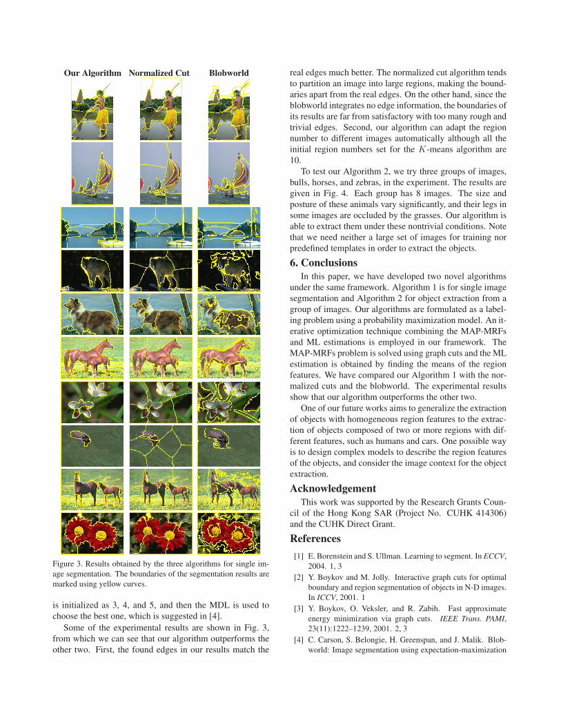
Our Algorithm Normalized Cut Blobworld

Figure 3. Results obtained by the three algorithms for single im-age segmentation. The boundaries of the segmentation results aremarked using yellow curves.

is initialized as 3, 4, and 5, and then the MDL is used tochoose the best one, which is suggested in [4].

Some of the experimental results are shown in Fig. 3,from which we can see that our algorithm outperforms theother two. First, the found edges in our results match the

real edges much better. The normalized cut algorithm tendsto partition an image into large regions, making the bound-aries apart from the real edges. On the other hand, since theblobworld integrates no edge information, the boundaries ofits results are far from satisfactory with too many rough andtrivial edges. Second, our algorithm can adapt the regionnumber to different images automatically although all theinitial region numbers set for the K-means algorithm are10.

To test our Algorithm 2, we try three groups of images,bulls, horses, and zebras, in the experiment. The results aregiven in Fig. 4. Each group has 8 images. The size andposture of these animals vary significantly, and their legs insome images are occluded by the grasses. Our algorithm isable to extract them under these nontrivial conditions. Notethat we need neither a large set of images for training norpredefined templates in order to extract the objects.

6. ConclusionsIn this paper, we have developed two novel algorithms

under the same framework. Algorithm 1 is for single imagesegmentation and Algorithm 2 for object extraction from agroup of images. Our algorithms are formulated as a label-ing problem using a probability maximization model. An it-erative optimization technique combining the MAP-MRFsand ML estimations is employed in our framework. TheMAP-MRFs problem is solved using graph cuts and the MLestimation is obtained by finding the means of the regionfeatures. We have compared our Algorithm 1 with the nor-malized cuts and the blobworld. The experimental resultsshow that our algorithm outperforms the other two.

One of our future works aims to generalize the extractionof objects with homogeneous region features to the extrac-tion of objects composed of two or more regions with dif-ferent features, such as humans and cars. One possible wayis to design complex models to describe the region featuresof the objects, and consider the image context for the objectextraction.

AcknowledgementThis work was supported by the Research Grants Coun-

cil of the Hong Kong SAR (Project No. CUHK 414306)and the CUHK Direct Grant.

References

[1] E. Borenstein and S. Ullman. Learning to segment. In ECCV,2004. 1, 3

[2] Y. Boykov and M. Jolly. Interactive graph cuts for optimalboundary and region segmentation of objects in N-D images.In ICCV, 2001. 1

[3] Y. Boykov, O. Veksler, and R. Zabih. Fast approximateenergy minimization via graph cuts. IEEE Trans. PAMI,23(11):1222–1239, 2001. 2, 3

[4] C. Carson, S. Belongie, H. Greenspan, and J. Malik. Blob-world: Image segmentation using expectation-maximization

Figure 4. Results of our algorithm for the extraction of objects from two groups of images. The first, third, and fifth column include 8 bullimages, horse images and zebra images respectively. The second, fourth, and sixth column are the extracted animals.

and its application to image querying. IEEE Trans. PAMI,24(8):1026–1038, 2002. 1, 2, 4, 5

[5] R. Duda, P. Hart, and D. Stork. Pattern Classification. Wiley-Interscience, 2 edition, 2001. 3

[6] W. Forstner. A framework for low level feature extraction.In ECCV, 1994. 2

[7] J. Garding and T. Lindeberg. Direct computation of shapecues using scale-adapted spatial derivative operators. IJCV,17(2):163–191, 1996. 2

[8] V. Kolmogorov and R. Zabih. What energy functions can beminimized via graph cuts? IEEE Trans. PAMI, 26(2):147–159, 2004. 1

[9] M. P. Kumar, P. H. S. Torr, and A. Zisserman. Obj cut. CVPR,2005. 1, 3

[10] A. Opelt, A. Pinz, and A. Zisserman. A boundary-fragment-model for object detection. In ECCV, 2006. 1, 3

[11] A. Opelt, A. Pinz, and A. Zisserman. Incremental learningof object detectors using a visual shape alphabet. In ICCV,

2006. 1, 3[12] T. Pappas. An adaptive clustering algorithm for image seg-

mentation. IEEE Trans. Signal Processing, 40(4):901–914,1992. 1

[13] J. Shi and J. Malik. Normalized cuts and image segmenta-tion. IEEE Trans. PAMI, 22(8):888–905, 2000. 1, 4

[14] Z. Tu and S.-C. Zhu. Image segmentation by data-drivenmarkov chain monte carlo. IEEE Trans. PAMI, 24(5):657–673, 2002. 1

[15] L. Vincent and P. Soille. Watersheds in digital spaces: Anefficient algorithm based on immersion simulations. IEEETrans. PAMI, 13(6):583–598, 1991. 1

[16] S. X. Yu and J. Shi. Multiclass spectral clustering. In ICCV,2003. 1

[17] R. Zabih and V. Kolmogorov. Spatially coherent clusteringusing graph cuts. In CVPR, 2004. 1