1

It’s Raining Men! Hallelujah?

Pauline Grosjean and Rose Khattar*

8 September 2014

Abstract

We document the implications of missing women in the short and long run. We exploit a

natural historical experiment, which sent large numbers of male convicts and far fewer

female convicts to Australia in the 18th

and 19th

century. In areas with higher sex ratios,

women historically married more, worked less, and were less likely to occupy high-rank

occupations. Today, people have more conservative attitudes towards women working,

women are still less likely to have high-ranking occupations, and they earn lower wages.

We document the role of vertical cultural transmission and of marriage homogamy in

sustaining cultural persistence. Our results are robust to controlling for a wide array of

geographic and historical controls, which determined spatial variation in the sex ratio, as

well as present-day controls and to instrumenting the overall sex ratio by the sex ratio

among convicts.

Keywords: Culture, gender roles, sex ratio, natural experiment, Australia

JEL codes: I31, N37, J16, Z33

* University of New South Wales. Corresponding author: Pauline Grosjean, School of Economics,

UNSW, Sydney NSW 2052, Australia. p.grosjean@unsw.edu.au. We are grateful to Chris Bidner,

Alison Booth, Monique Borgerhoff-Mulder, Sam Bowles, Rob Boyd, Rob Brooks, Raquel

Fernandez, Gigi Foster, Gabriele Gratton, Ralph de Haas, Kim Hill, Hongyi Li, Leslie Martin,

Suresh Naidu, Paul Seabright, Jesse Shapiro, Peter Siminski, and audiences at the NBER Summer

Institute Political Economy 2014, Australian National University, the Institute for Advanced

Studies in Toulouse, Hong Kong UST, Monash University, the Santa Fe Institute, Sciences-Po,

University of Sydney, UNSW and Wollongong University for comments and suggestions. We

thank Renee Adams for financial help with this project. This paper uses unit record data from the

Household, Income and Labor Dynamics in Australia (HILDA) Survey. The HILDA Project was

initiated and is funded by the Australian Government Department of Families, Housing,

Community Services and Indigenous Affairs (FaHCSIA) and is managed by the Melbourne

Institute of Applied Economic and Social Research (Melbourne Institute). The findings and views

reported in this paper, however, are those of the authors and should not be attributed to either

FaHCSIA or the Melbourne Institute. All errors and omissions are the authors’.

2

1. Introduction

Traditional economic models link the division of labor between men and women to the

available technology, which determines the relative returns to male and female labor, and

to the conditions in the marriage market, which determine the outcome of bargaining

between men and women. However, recent work has highlighted the importance of

cultural norms and beliefs about appropriate gender roles (Fernandez 2009, 2013,

Bertrand, Kamenica, and Pan 2013). This opens the question of how such beliefs emerge

and persist. To answer this question, Alesina, Giuliano and Nunn (2013) point to the

technology that was available in pre-industrial times. Past technology still matters, the

authors argue, because it shaped the division of labor between men and women, which

was then integrated into cultural norms that persisted over time. Taking a natural step, we

ask whether, and how, past shocks to the marriage market have similarly enduring effects.

We exploit variation in marriage markets conditions that arose from an exogenous

variation in the sex ratio among an otherwise homogeneous population. Heavily male

biased sex ratios resulted from British policy to send convicts to Australia in the late 18th

and 19th

century. Men far outnumbered women among convicts, by a ratio of 6 to 1

(Oxley 1996). Free migration to Australia in the 19th

century and the beginning of the 20th

century was also heavily male biased, as mostly men were seeking out economic

opportunities in mining and pastoralism. As can be seen in Figure 1, a male biased sex

ratio endured in Australia for more than a century.

We rely spatial and time variation in the historical sex ratio. Historically, gender

imbalance was associated with women marrying more, participating less in the labor

force, and being less likely to work in high-ranking occupations. We then study the long-

term implications by matching, for the first time, 91 historical counties from the

Australian Colonial Censuses to postal areas in the 1933 Census, the 2011 Census and in

a nationally representative household survey collected between 2001 and 2011. In areas

that had a larger imbalance historically, people today have more conservative attitudes

towards women working, women are less likely to have high-ranking occupations, and

they receive lower wages. However, we find no evidence that the overall effect on

3

women’s welfare is negative, as measured by self-reported satisfaction or in time use data.

The “glass ceiling” effect was already present, and larger in magnitude in 1933, before

the onset of large migration flows to Australia after the Second World War.

A one unit increase in the historical sex ratio -one more man for a given number of

women- moves the average Australian today towards conservative attitudes by 6% at the

mean. This additional man is also associated with a 1 percentage point decrease in the

share of women employed as professionals, which represents nearly 5% of the population

mean and 12% of its standard deviation. Historical circumstances explain 5% of the

variation in the share of women employed as professionals that is left unexplained by

traditional factors, even when accounting for the share of men employed in similar

professions. Moving from a sex ratio at parity to the historical mean of 3 is associated

with a 6% increase in the gender pay gap today.

A concern for identification is that gender imbalance across localities was determined by

characteristics that also influence our outcomes of interest. Our historical results are

robust in a panel of historical counties, controlling for time and county fixed effects,

which remove the influence of any time invariant county characteristics that could be

associated both with local gender imbalance and with female work outcomes. Results

pertaining to the legacy of the sex ratio on present day outcomes are only available in a

cross section, so that we cannot pursue a similar strategy. Instead, we start by carefully

analyzing the characteristics that determined the allocation of men and women across

counties and control for such factors in the regression analysis. To account for the

influence of economic opportunities, which consisted chiefly of agriculture, pastoralism,

as well as mining, we control flexibly for geographic characteristics by including latitude

and longitude in all specifications, and we control precisely for the presence of minerals

and for terrain characteristics, as well as for the initial conditions in the county in terms

of economic specialization. We also account for a wide range of individual and

contemporary controls as well as state fixed effects throughout, which remove any

unobserved heterogeneity due to differences in the legal environment or in the treatment

of convicts.

4

Although we are able to account for the influence of a large number of geographic and

historical characteristics, it remains possible that local gender imbalance in the past was

influenced by unobservable characteristics that still underlie female opportunities as well

as attitudes in the present. Endogeneity could arise, for example, from the systematic

selection of women with stronger preferences for leisure or of men with a taste of

discrimination against women to high historical sex ratio areas. To deal with this, we

employ an instrumental variable strategy based on a unique feature of Australia’s history:

convict transportation from Britain. All the results are robust to instrumenting the overall

sex ratio by the sex ratio among convicts. Although convicts had no choice where to

locate, they were not confined to prisons. They either worked under the government’s

supervision or were assigned to employers, who were either free settlers or former

convicts. As before, we remove the potential endogeneity that arises from this process of

convict assignment by controlling for the abovementioned geographic and historical

controls. Since a legacy of a convict past independent of gender imbalance would violate

the exclusion restriction, we also control for the number of convicts.

We undertake a number of additional robustness tests. In particular, we check that the

results do not rely on a specific measure of the sex ratio at one point in time. The results

are also robust to propensity score matching on the basis of geographic and historical

characteristics. Placebo specifications, in which sex ratios are randomly allocated across

counties while keeping the overall imbalance unchanged, give no significant results. The

results are also specific to views about women working; historical gender imbalance does

not explain sexism in general proxied by other survey questions on attitudes towards

women.

Our historical results, contemporaneous to gender imbalance, are in line with previous

literature. Economic and evolutionary biology models predict more conservative gender

roles as a result of male-biased sex ratios (Grossbard-Schechtman 1984, Chiappori 1988,

1992, Chiappori, Fortin and Lacroix 2002, Kokko and Jennions 2008). This is

particularly relevant when job opportunities for women are few or unattractive, as it was

the case in 19th

century Australia, which was heavily specialized in the production of

primary commodities.

5

What may be more surprising is that this effect has persisted to this day, after sex ratios

have reverted back to parity. To explain persistence, we argue that past gender imbalance

has shaped cultural beliefs about gender roles. We first rule out that other mechanisms

explain persistence. Our results rely on within-country and even within-state variation,

where formal legislation is identical1, which rules out formal institutions as a persistence

mechanism. Another possibility is that past circumstances in the marriage market

influenced respective incentives of men and women to invest in education (Chiappori,

Iyigun, and Weiss 2009). We find no evidence for this mechanism. Initial gender

imbalance could also have distorted industrial specialization towards male-intensive

economic activities. Since we control for geographical endowments, such as land

characteristics and mineral discoveries, and for initial economic specialization, we view

the remaining variation as integrant to cultural persistence. We also analyze local

historiographies and document differences today between areas that had and still have a

similar economic specialization but different past sex ratios.

We next investigate the channels that underlie cultural persistence. Culture persists

because of the transmission of cultural traits within families (vertical) or across unrelated

individuals (horizontal) (Cavalli-Sforza 1981, Bisin and Verdier 2001, Hauk and Saez-

Marti 2002). We find, consistent with vertical transmission, that historical gender

imbalance is only associated with conservative views about gender roles among people

born of an Australian father.

Our focus on the marriage market suggests an additional persistence mechanism.

Assortative mating makes gender norms strategic complements among potential spouses.

Strategic complementarity implies that norms become evolutionary stable (Young 1998)

and that even inferior conventions can persist over time, as shown theoretically by

Tabellini (2008) and Belloc and Bowles (2013). Accordingly, we find that historical

1 The legal framework operating in Australia with respect to gender discrimination has been

constant across all states since the Sex Discrimination Act 1984 (Cth), which operates at a federal

level. This is a direct consequence of Australia’s Constitution, with any state law inconsistent

with this act invalid to the extent of the inconsistency (Constitution s 109). The Family Law Act

1975 (Cth) unifies family law in Australia at this federal level.

6

gender imbalance is only associated with conservative gender views in areas where

homogamy is high.

The main contributions of this paper are two-fold. The first is to shed light on the long-

term effects of gender imbalance. The effects of gender imbalance norms and female

occupations persist for more than a hundred years, even though sex ratios have long

reverted to normal. This has important implications for the world today, where it has been

estimated that a hundred million women are missing (Hesketh and Xing 2006), namely in

China, India, sub-Saharan Africa and the Caucasus.2 The study of the determinants of

such gender imbalances has attracted a large literature.3 The study of its consequences is

more limited because of evident reverse causality issues. We discuss this literature in

more detail in Section 2 of this paper.

Our second contribution is to the literature on the influence of culture on economic

outcomes and, more precisely, on how culture emerges and persists. Until recently, the

rise in female labor force participation, the expansion of women’s economic and political

rights, as well as the reduction in fertility that has been observed in developed countries

were explained by technological change and the rise in returns to female labor.4 However,

several studies have also demonstrated how slow-changing cultural beliefs influence real

work choices, family formation and welfare.5 Regarding the origins of such beliefs,

Alesina, Giuliano and Nunn (2013) show that conservative gender norms stem from the

introduction of plough agricultural in pre-industrial societies. Our contribution is to

illustrate a more rapid cultural change, which took place within a homogenous population

and to document how a large shock in the marriage market can shape cultural beliefs and

have persistent effects in the long run.

2 See Anderson and Ray (2010) for sub-Saharan Africa and Brainerd (2013) for the Caucasus.

3 See Rao (1993), Hesketh and Xing (2006), Chung and Das Gupta (2007), Edlund and Lee

(2009). 4 See namely Goldin and Katz (2002), Greenwood, Seshadri and Vandenbroucke (2005), Doepke

and Tertilt (2009), Doepke, Tertilt and Voena (2012), Olivetti (2013). 5 Fortin (2005) shows how gender role attitudes influence labor market outcomes. Alesina,

Giuliano and Nunn (2013) establish a relationship between beliefs and participation of women in

the economy and in politics. Bertrand, Pan and Kamenica (2013) find that households in which

women earn more than men are less likely to form and, once formed, are more likely to lead to

divorce. Fernandez (2008) and Fernandez and Fogli (2009) show that preferences for fertility and

for female labor force participation change slowly

7

2. Conceptual Background

In this section, we explain how a large shock to the marriage market, with a large excess

of males, can move social norms towards more conservative views of gender roles. We

also discuss how society can remain stuck in this new equilibrium, despite subsequent,

smaller changes in gender ratios.

Work by economists, social psychologists, and evolutionary biologists predict that a male

biased sex ratio will result in conservative gender roles. Economic marriage models

predict that the bargaining position of one gender is proportional to its scarcity (Becker

1973, 1974). Accordingly, Pollet and Nettle (2008) find that the importance of men’s

wealth for marriage in the US at the beginning of the 20th

century is positively correlated

with local sex ratios. Addressing the possible endogeneity between local marriage

conditions and local sex ratios, Abramitzky, Delavande and Vasconcelos (2011) exploit

variation in World War I related deaths in France. They find that a shortage of men is

associated with men marrying more and marrying up. In the case of Taiwan after the

influx of the Chinese Nationalist Army in 1949, Francis (2011) shows that, conversely, a

shortage of women leads to women marrying more. An improvement in women’s

bargaining position resulting from higher sex ratios is also predicted to reduce female

labor force participation (Grossbard-Schechtman 1984, Chiappori 1988, 1992, Chiappori,

Fortin and Lacroix 2002). This is supported by empirical evidence based on the influence

of contemporaneous changes in the sex ratios of recent migrants on the outcomes of

second-generation migrants (Angrist 2002).

Guttentag and Secord (1983) relate sex ratios and women’s status and roles based on a

similar idea that women have greater bargaining power when there are fewer of them

around. However, they note that when political and economic power resides in the hands

of men, the ability of women to use their bargaining power to gain freedom and

independence is limited. In particular, they predict that in high sex ratios societies,

women’s extra-familial roles will be limited, although women will be treated with more

8

respect and greatly valued in their roles as homemakers and, as a result of being so highly

valued, will be content and less prone to suicide (Guttentag and Secord 1983, p. 20).

While this work puts forward bargaining as the main mechanism through which the sex

ratio affects gender roles, evolutionary biologists discuss others. Males may respond to

competitive pressures by making themselves more attractive to females, which involves

resource transfers as in bargaining models, but not only (Kokko and Jennions 2008).

Male-biased sex ratios may have negative consequences for females when males divert

resources from the female and offspring towards competing with other males, or when

males engage in mate guarding and restrict female freedom. Regardless, the prediction

applied to humans is still that male-biased sex ratios will lead to more conservative

gender roles with females working less outside the home.

As argued by Alesina, Giuliano and Nunn (2013), conservative gender roles and low

female labor force participation imprint onto cultural norms about the appropriate role of

women in society. Gender roles of the past then persist in the long run because culture

changes slowly. Culture is defined, after Richersen and Boyd (2008), as “rules of thumb”

that affect behavior in complex and uncertain environments and that people acquire from

other people through “teaching, imitation and other forms of social transmission”

(Richersen and Boyd 2008, p. 5). Cultural traits that are successful, which in our context

means getting a wife, will spread.

The economic literature discusses two main channels of cultural transmission: horizontal

and vertical (Cavalli-Sforza 1981, Bisin and Verdier 2001). Culture spreads horizontally

across peers, mainly through imitation. Culture spreads vertically from parents to

children, through imitation and active parental socialization (Bisin and Verdier 2001,

Doepke and Zilibotti 2008). Vertical transmission is inherently sticky. The implied

hysteresis explains why historical sex ratios may have persistent effects, even long after

sex ratios have reverted back to normal.

Our focus on the marriage market suggests an additional persistence mechanism.

Assortative mating on the marriage market implies that views about gender roles are

strategic complements among potential spouses. More similar individuals are more likely

9

to be married to each other and more likely to stay married (Becker et al. 1977, Heaton

1984, Lehrer-Chiswick 1993). In the marriage market, if certain norms make matching

more likely, and a match more successful, they will prevail and persist over time.

Conservative gender roles may thus persist in the long run solely because they are mutual

best responses in a homogamous marriage market. Young (1998) shows theoretically that

norms that are mutual best responses are evolutionary stable. Positive feedbacks of this

kind are at the core of the persistence of cultural conventions in Belloc and Bowles

(2013), even when such conventions are Pareto-dominated. Thus, conservative cultural

traits may persist even when they are no longer adaptive once the sex ratio has reverted

back to normal and economic opportunities for women have improved.

Belloc and Bowles (2013) discuss conditions that make the transition from one

convention to another more likely. Cultural change has the characteristics of a collective

action problem. The greater the cost of deviating from a given set of cultural traits and

the bigger the population size, the less likely it is that any cultural change will occur.

Deviation and experimentation may be particularly costly in the marriage market, where

time is of the essence, uncertainty substantial, and search costs relatively high. If holding

modern views leads to long delays in finding a spouse, people will conserve traditional

views. However, immigration should make experimentation easier and may accelerate

transition towards modern gender views. Conversely, homogamy in the marriage market,

a proxy for the strength of strategic complementarity of gender views, should be

associated with stronger persistence of norms. Homogamy will interact with vertical

transmission in a very natural way, as discussed in Bisin, Topa and Verdier (2004).

Parents want to instill in their children norms that will make them attractive in the

marriage market. If they anticipate that the prevalence of conservative gender views is

high among potential spouses, parents will try harder to transmit such views to their

children. We are able to test all of these predictions in the empirical analysis that follows.

10

3. Historical Background, Data, and Results: Gender Imbalance, Female Work and

Marriage in 19th

Century Australia

3.1. Historical Background

European settlement in Australia commenced after independence of the United States,

when it became the new destination of choice for the United Kingdom’s overflowing jail

population. Between 1787 and 1868, 132,308 and 24,960 convict men and women were

transported to Australia, mostly to Tasmania and New South Wales (hereafter, NSW),

which initially also included Queensland, the Australian Capital Territory, and Victoria

(Oxley 1996, p. 3). These convict men and women were not “hardened and professional

criminals” (Nicholas et al 1988, p. 3) but “ordinary working class men and women”

(Nicholas et al 1988, p. 7): the majority of convicts were transported for property

offences, such as petty theft (Oxley 1996).

The extent of free migration to Australia was rather limited until the 1830s and the

imbalance was sustained by ongoing convict transportation for nearly a century. Male

convicts made up more than 80% of the adult male population of NSW in 1833. Even

among free migrants, men outnumbered women. It was mainly men who were attracted

by economic opportunities in Australia, which consisted mainly of pastoralism and

mining, especially after the discovery of gold in the beginning of the 1850s. As can be

seen in Figure 1, a male biased sex ratio endured in Australia for more than a century.

The settler population of Australia was ethnically homogenous. The vast majority of

convicts and free migrants came from England and Ireland. In the 1846 NSW Census,

about 50% of people born outside the colony came from England and 40% from Ireland.

There was very little heterogeneity across different localities within Australia: the

standard deviation of the two distributions is only 0.05.

Essential to our identification strategy is to understand what determined the variation in

population and sex ratios across space. Upon arrival, convicts were not confined to prison

cells. Initially, they were assigned to work under government supervision. Later, as the

cost of caring for large numbers of convicts became too high, convicts were assigned for

11

private employment. Employers were government officials, free settlers, or ex-convicts.

The placement of convicts was dictated purely by labor requirements and decided in a

highly centralized way, as described by Governor Bligh of NSW in 1812:

“They (the convicts) were arranged in our book (…) in order to enable me to

distribute them according” (cited in Nicholas 1988, p. 15, emphasis added).

As for free settlers, their spatial distribution was determined also by economic

opportunities, namely in agriculture and mining, the two sectors in which Australia

specialized in the 19th

century (McLean 2013).

Male labor was at a high premium in the colonial economy. Wages were set by the

government and in 1816, Governor Macquarie of NSW announced that male and female

convicts must be paid £10 and £7 per annum, respectively (Nicholas et al 1988, p. 131).

Meredith and Oxley (2005, p. 56) document an even larger, 46%, gender pay gap in the

general population. One explanation is that only men had the physical strength required

for agricultural work and building the country (Nicholas et al 1988). Alford (1984, p.

243) also suggests that the notion that remaining within the home was a “woman’s proper

place” played, already, a large role in explaining why women were “undervalued and

underemployed” in the labor market (Nicholas et al 1988, p. 15).

Some convict women were confined to female factories.6 Female factories were “a

combination of textile factory and female prison” (Salt 1984, p. 142) for women who had

borne a child out of wedlock, displeased their assigned master, or committed a crime.

Women worked in female factories for a very low or no wage.7 Overall, Governor

Macquarie of NSW put it best when he stated that convict women had 3 choices: become

a domestic servant, live in a female factory, or marry (Alford 1984, p. 29). In the

circumstances described above, together with a high demand for wives, marriage seemed

like the most attractive option.

6 No analogous male factory existed. NSW had 3 female factories in the counties of Cumberland,

Northumberland and Macquarie. Queensland’s county of Brisbane had 1 and Tasmania 5; 2

located in Hobart and the rest in Launceston, George Town and Campbell Town. 7 Third class women, those who committed a crime in the colony or misbehaved in the factory,

received no wage (Salt 1984, pp. 86, 105).

12

The authorities’ concern that “the disproportion of the sexes” would have “evil effects”

as men experienced “difficulty … in getting wives” (Select Committee on Transportation

1837-1838, p. xxvii) was well founded. Men were more than half as likely to be married

than women (see Table 1), who were under great pressure to be married. According to the

historical Census, more than 70% of women in Australia were married in the 19th

century,

a much higher rate than in Britain at the same time period (60%) (Alford 1984, p. 26).

The legal ability to divorce came rather late, particularly in NSW (1873). By the end of

the 19th

century (1892), there were a total of only 799 divorce petitions in NSW (Golder

1985). Also, marriage was enforced by authorities. For example, bearing a child out of

wedlock was considered a crime for which women could be sent to prison.

In sum, 19th

century Australia was a context in which women’s economic opportunities

outside marriage were limited and unattractive and in which the opportunity cost of a bad

match was high because of the difficulty of divorcing. In this context, it is expected that

women will be attracted to men who can fulfill the role of economic provider. Bargaining

also predicts that women will work less, particularly in such an environment in which

female labor was arduous and poorly rewarded.

3.2. Historical Data

We collect data on the historical gender ratio and on the structure of the colonial

economy from the Colonial Censuses taken in the 19th

century in each of the six

Australian states.8 Other data sources, such as colonial musters that counted transported

people, have high reporting error and are not representative of the entire population since

participation was not compulsory (Camm 1978, p. 112).

Our measure of the historical sex ratio in regressions with present day outcomes is taken

from the first Census in each state, because we want to rely on the earliest possible

measure of the gender imbalance and of its exogenous component, which came from

convict transportation. We therefore rely mostly on the 1836 NSW Census (which also

8 The online data from the Historical Census and Colonial Data Archive was supplemented by the

actual Census report due to errors in the 1881 Tasmanian Census. Only the Census reports are

available consistently across the period, as some of the individual records have burned.

13

included the Australian Capital Territory at the time), the 1842 Tasmanian Census, the

1844 South Australian Census, the 1848 Western Australian Census, the 1854 Victorian

Census, and the 1861 Queensland Census. These dates vary because states were

independent colonies until 1901. Figure A1 in Appendix contains more detail on these

data sources.

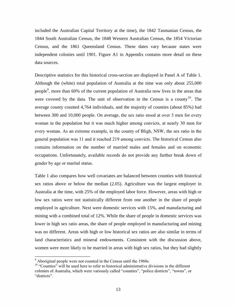
Descriptive statistics for this historical cross-section are displayed in Panel A of Table 1.

Although the (white) total population of Australia at the time was only about 255,000

people9, more than 60% of the current population of Australia now lives in the areas that

were covered by the data. The unit of observation in the Census is a county10

. The

average county counted 4,764 individuals, and the majority of counties (about 85%) had

between 300 and 10,000 people. On average, the sex ratio stood at over 3 men for every

woman in the population but it was much higher among convicts, at nearly 30 men for

every woman. As an extreme example, in the county of Bligh, NSW, the sex ratio in the

general population was 11 and it reached 219 among convicts. The historical Census also

contains information on the number of married males and females and on economic

occupations. Unfortunately, available records do not provide any further break down of

gender by age or marital status.

Table 1 also compares how well covariates are balanced between counties with historical

sex ratios above or below the median (2.05). Agriculture was the largest employer in

Australia at the time, with 25% of the employed labor force. However, areas with high or

low sex ratios were not statistically different from one another in the share of people

employed in agriculture. Next were domestic services with 15%, and manufacturing and

mining with a combined total of 12%. While the share of people in domestic services was

lower in high sex ratio areas, the share of people employed in manufacturing and mining

was no different. Areas with high or low historical sex ratios are also similar in terms of

land characteristics and mineral endowments. Consistent with the discussion above,

women were more likely to be married in areas with high sex ratios, but they had slightly

9 Aboriginal people were not counted in the Census until the 1960s.

10 “Counties” will be used here to refer to historical administrative divisions in the different

colonies of Australia, which were variously called “counties”, “police districts”, “towns”, or

“districts”.

14

fewer children, which could be taken as an indication that they exerted higher bargaining

power.

Figures 2 and 3 map the sex ratio among the general and convict populations. The

population included in the historical Census came to Australia by sea. Yet, by the time we

measure them, people of both sexes had made their way into the hinterland and along the

coasts. The concentration of sexes has no definite pattern: high and low sex ratios were

found in the hinterland as well as along the coast.

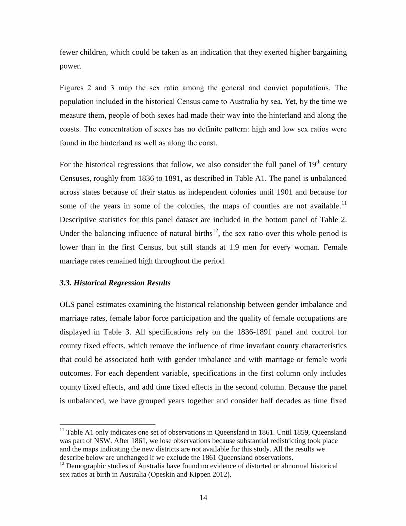
For the historical regressions that follow, we also consider the full panel of 19th

century

Censuses, roughly from 1836 to 1891, as described in Table A1. The panel is unbalanced

across states because of their status as independent colonies until 1901 and because for

some of the years in some of the colonies, the maps of counties are not available.11

Descriptive statistics for this panel dataset are included in the bottom panel of Table 2.

Under the balancing influence of natural births12

, the sex ratio over this whole period is

lower than in the first Census, but still stands at 1.9 men for every woman. Female

marriage rates remained high throughout the period.

3.3. Historical Regression Results

OLS panel estimates examining the historical relationship between gender imbalance and

marriage rates, female labor force participation and the quality of female occupations are

displayed in Table 3. All specifications rely on the 1836-1891 panel and control for

county fixed effects, which remove the influence of time invariant county characteristics

that could be associated both with gender imbalance and with marriage or female work

outcomes. For each dependent variable, specifications in the first column only includes

county fixed effects, and add time fixed effects in the second column. Because the panel

is unbalanced, we have grouped years together and consider half decades as time fixed

11

Table A1 only indicates one set of observations in Queensland in 1861. Until 1859, Queensland

was part of NSW. After 1861, we lose observations because substantial redistricting took place

and the maps indicating the new districts are not available for this study. All the results we

describe below are unchanged if we exclude the 1861 Queensland observations. 12

Demographic studies of Australia have found no evidence of distorted or abnormal historical

sex ratios at birth in Australia (Opeskin and Kippen 2012).

15

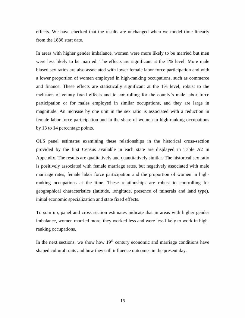
effects. We have checked that the results are unchanged when we model time linearly

from the 1836 start date.

In areas with higher gender imbalance, women were more likely to be married but men

were less likely to be married. The effects are significant at the 1% level. More male

biased sex ratios are also associated with lower female labor force participation and with

a lower proportion of women employed in high-ranking occupations, such as commerce

and finance. These effects are statistically significant at the 1% level, robust to the

inclusion of county fixed effects and to controlling for the county’s male labor force

participation or for males employed in similar occupations, and they are large in

magnitude. An increase by one unit in the sex ratio is associated with a reduction in

female labor force participation and in the share of women in high-ranking occupations

by 13 to 14 percentage points.

OLS panel estimates examining these relationships in the historical cross-section

provided by the first Census available in each state are displayed in Table A2 in

Appendix. The results are qualitatively and quantitatively similar. The historical sex ratio

is positively associated with female marriage rates, but negatively associated with male

marriage rates, female labor force participation and the proportion of women in high-

ranking occupations at the time. These relationships are robust to controlling for

geographical characteristics (latitude, longitude, presence of minerals and land type),

initial economic specialization and state fixed effects.

To sum up, panel and cross section estimates indicate that in areas with higher gender

imbalance, women married more, they worked less and were less likely to work in high-

ranking occupations.

In the next sections, we show how 19th

century economic and marriage conditions have

shaped cultural traits and how they still influence outcomes in the present day.

16

4. The legacy of gender imbalance on culture and on women in the workplace

In this section, we explore the long-term consequences of gender imbalance for female

labor force participation and occupational choices and how it has shaped the cultural

values of Australians. First, we discuss how we link historical gender imbalance to

present-day opinion surveys and Census data.

4.1.Data

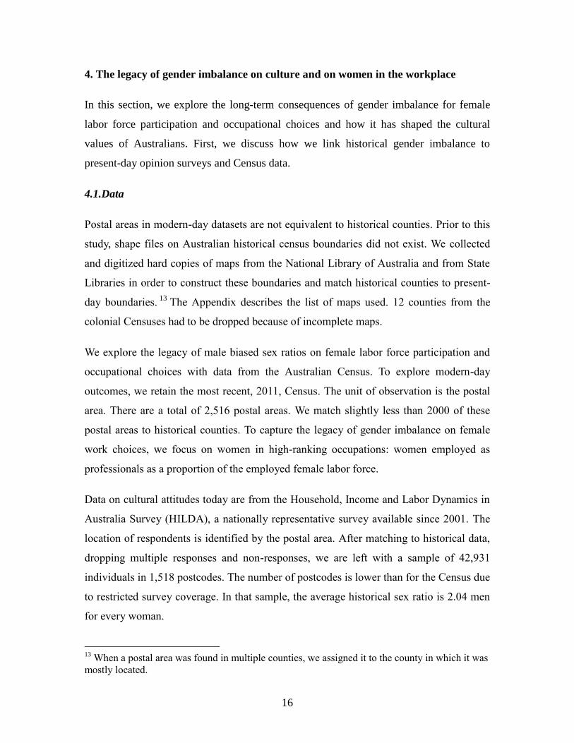
Postal areas in modern-day datasets are not equivalent to historical counties. Prior to this

study, shape files on Australian historical census boundaries did not exist. We collected

and digitized hard copies of maps from the National Library of Australia and from State

Libraries in order to construct these boundaries and match historical counties to present-

day boundaries. 13 The Appendix describes the list of maps used. 12 counties from the

colonial Censuses had to be dropped because of incomplete maps.

We explore the legacy of male biased sex ratios on female labor force participation and

occupational choices with data from the Australian Census. To explore modern-day

outcomes, we retain the most recent, 2011, Census. The unit of observation is the postal

area. There are a total of 2,516 postal areas. We match slightly less than 2000 of these

postal areas to historical counties. To capture the legacy of gender imbalance on female

work choices, we focus on women in high-ranking occupations: women employed as

professionals as a proportion of the employed female labor force.

Data on cultural attitudes today are from the Household, Income and Labor Dynamics in

Australia Survey (HILDA), a nationally representative survey available since 2001. The

location of respondents is identified by the postal area. After matching to historical data,

dropping multiple responses and non-responses, we are left with a sample of 42,931

individuals in 1,518 postcodes. The number of postcodes is lower than for the Census due

to restricted survey coverage. In that sample, the average historical sex ratio is 2.04 men

for every woman.

13

When a postal area was found in multiple counties, we assigned it to the county in which it was

mostly located.

17

Questions on attitudes towards gender roles were included in the 2001, 2005, 2008 and

2011 waves. The main question that captures views about gender roles asks to what

extent respondents agree that: “it is better for everyone involved if the man earns the

money and the woman takes care of the home and children.” Response categories range

from 1 (strongly disagree) to 7 (strongly agree). We recoded this so that a higher value

indicates stronger disagreement with this statement, which we interpret as the respondent

holding more progressive attitudes.

We retain several individual characteristics from HILDA and from the Census as controls.

Descriptive statistics are provided in Panels B and C of Table 1. The balance of these

covariates across areas below or above the median historical sex ratio is also presented in

the last 2 Columns of Table 1. We observe no statistically significant difference across

high and low historical sex ratio areas in terms of age, gender, ancestry composition,

income, education, or gender balance today. Areas that were more imbalanced

historically tend to be more rural today, although the difference is only barely statistically

significant at the 10% level. Still, we will include whether a postal area is urban as a

control.

4.2. Specifications and OLS results

Having matched historical gender imbalance to postal areas, we are able to examine its

legacy on attitudes, female labor force participation and occupational choices. Figure A2

in the Appendix shows that progressive attitudes towards gender roles, female labor force

participation, and the proportion of women employed in high-ranking occupations are all

negatively correlated with the historical sex ratio. The unconditional relationships

between all three outcomes and the historic sex ratio are all significant at the 1% level

and robust to the removal of outliers, such as areas with more than 10 men for every one

woman. The simple correlation coefficients between these variables stand well above the

0.1 mark considered in Chatelain and Ralf (2014) as critical in regards to the possibility

of spurious regression.14

14

The correlation coefficients between, on the one hand, the historical sex ratio and, on the other

hand, progressive attitudes and female labor force participation are -0.25. The correlation

18

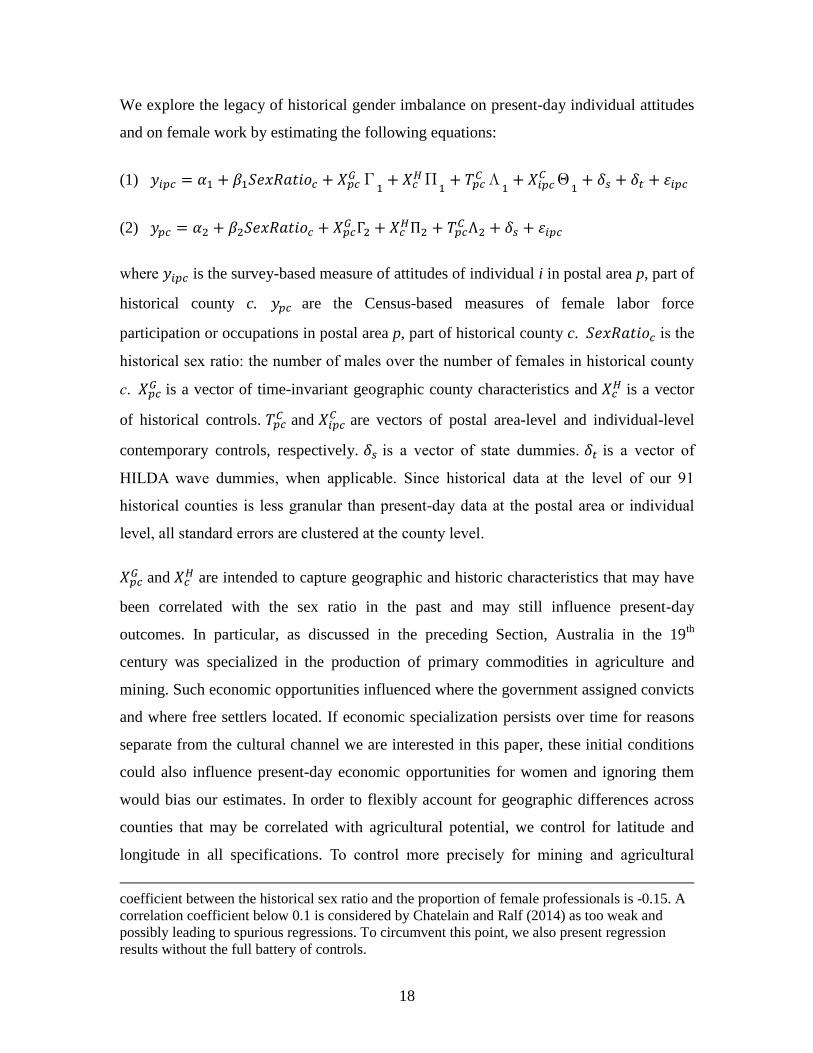
We explore the legacy of historical gender imbalance on present-day individual attitudes

and on female work by estimating the following equations:

(1) Γ

Π

Λ

Θ

(2)

where is the survey-based measure of attitudes of individual i in postal area p, part of

historical county c. are the Census-based measures of female labor force

participation or occupations in postal area p, part of historical county c. is the

historical sex ratio: the number of males over the number of females in historical county

c. is a vector of time-invariant geographic county characteristics and

is a vector

of historical controls. and

are vectors of postal area-level and individual-level

contemporary controls, respectively. is a vector of state dummies. is a vector of

HILDA wave dummies, when applicable. Since historical data at the level of our 91

historical counties is less granular than present-day data at the postal area or individual

level, all standard errors are clustered at the county level.

and

are intended to capture geographic and historic characteristics that may have

been correlated with the sex ratio in the past and may still influence present-day

outcomes. In particular, as discussed in the preceding Section, Australia in the 19th

century was specialized in the production of primary commodities in agriculture and

mining. Such economic opportunities influenced where the government assigned convicts

and where free settlers located. If economic specialization persists over time for reasons

separate from the cultural channel we are interested in this paper, these initial conditions

could also influence present-day economic opportunities for women and ignoring them

would bias our estimates. In order to flexibly account for geographic differences across

counties that may be correlated with agricultural potential, we control for latitude and

longitude in all specifications. To control more precisely for mining and agricultural

coefficient between the historical sex ratio and the proportion of female professionals is -0.15. A

correlation coefficient below 0.1 is considered by Chatelain and Ralf (2014) as too weak and

possibly leading to spurious regressions. To circumvent this point, we also present regression

results without the full battery of controls.

19

opportunities, we control for 9 detailed categories of mineral deposits15 and for land

characteristics.16 We have already discussed in the preceding section that high and low

sex ratios areas did not differ systematically from one another along any these

dimensions. We do not include elevation in our list of covariates because it shows very

little variation, with 95% of our population being in a low-grade area. We also control

directly for the county historical economic specialization, by including in the

historical shares of the population employed in the main categories of employment

discussed in Section 3: agriculture, domestic services, mining and manufacturing, as well

as in employment categories that could provide opportunities for women: government

and learned professions (including teaching). Total historical population is also included

in .

In the models of individual attitudes, present day individual controls include gender,

marital status, age, income, education, and whether the respondent was born in Australia.

Postal area-level controls include the sex ratio today, and the degree of urbanization. All

postal area-level controls are from the Census.

In the models of female labor force participation and occupational choice from the

Census, contemporary controls at the postal area include the sex ratio today, average

education, and the degree of urbanization. Controlling for the proportion of married

people or for the full range of industrial specialization is problematic, as these are

endogenous outcomes. However, to account for sectorial differences across counties that

influence the share of women employed as professionals, we control for the share of men

employed in a similar occupation. Considering that we are exploiting within-country and

even within-state variation, keeping the formal legislation constant, controlling for the

share of men employed in a similar occupation should leave us with the variation that is

due to culture, as opposed to formal institutions, technology, or employment

opportunities.

15

Minor coal; minor other; major coal; major copper; major gold; major mineral sands; major oil

and gas; major others. The excluded category is no deposits or traces only. Source: Geoscience

Australia. 16

Plains, plateaus and sand plains (the excluded category); hills and ridges; low plateaus and low

hills; mountains. Source: Geoscience Australia.

20

The estimates displayed in Table 3 show that where the gender imbalance was most

severe in the early days of colonial settlement in Australia, people are less likely to hold

progressive views about gender roles, and women are less likely to participate in the

labor force; when women do work, they are less likely to occupy high-ranking

occupations.

The relationship between attitudes towards gender roles and historical gender imbalance

remains statistically significant at the 1% level even when controlling for the full set of

geographic, historic, and contemporary controls. At the mean, one more man historically

for a given number of women moves the average Australian today towards conservative

attitudes by nearly 6 percentage points (2.04*0.03). The relationship between the

historical sex ratio and attitudes today is specific to views about women working. Gender

imbalance does not explain sexist attitudes in general. Table A3 includes the estimation

results of equation (1) in which the dependent variable captures respondents’ views about

the quality of female leaders. There is no significant relationship between historical

gender imbalance and such attitudes.

The relationship between female labor force participation and the historical sex ratio

remains negative but is no longer significant when we include all contemporary controls.

Female labor force participation may be too gross a measure as it pools together female

executives and check out chicks. When we focus on the quality of female work instead,

the relationship with historical gender imbalance remains statistically significant when

controlling for the full set of controls, including the share of men employed in similar

occupations. At the mean, one more man historically is associated with slightly under 1

percentage point decrease in the share of women employed as professionals, which

represents nearly 5% of the population mean and 12% of its standard deviation. In terms

of the share of the variation explained, adding historical characteristics to the full set of

controls increases the R-squared by 3 percentage points. This is equivalent to 3.5% of the

remaining unexplained variation in the share of women employed as professionals.17

17

This is calculated as (0.577-0.562) / (1-0.562). 0.562 is the R-squared of a regression with all

but historical controls.

21

All the results pertaining to attitudes and to the share in high ranking occupations are

robust to non linear effects of the historical sex ratio, to excluding metropolitan areas, and

to excluding counties that had fewer than 300 people or more than 40,000 people,

counties that had very few women historically (less than 100). They are also robust to

controlling for distance to major ports of entry and to the main metropolitan areas, to

controlling for population density today, or for the shares of different religions in the

population, historically and today.18

Some of these additional robustness tests are

presented in Table A4. We also check that the results are robust to propensity score

matching. We predict the historical sex ratio as a flexible function of extended

geographic characteristics (latitude, longitude, presence of minerals, land type) and

historical employment shares in different sectors as well as all interactions between

geographic and historical characteristics and second order polynomials, and condition on

this predicted propensity score in the main specification. All the results described so far

carry through (see Columns 6 and 13 of Table A4). Columns 7 and 14 of Table A4

display the results of placebo specifications in which historical sex ratios are randomly

re-allocated between historical counties, while keeping the overall share of men relative

to women constant. The results are not significant.

We also check that the results are not idiosyncratic to a specific measure of the historical

sex ratio at a particular point in time. In Table A5, we present similar specifications as in

Table 3 but we rely on a later measure of the sex ratio, in 1861, by which date the total

population of Australia had increased nearly 5 fold since 1840. The 1861 sex ratio stood

at an average of 1.71 men for every one woman. The specifications, set of controls, and

results in Table A5 are identical to those in Table 3.

4.3. Instrumental variable results

Our results are robust to a battery of observable geographic, historical, and contemporary

controls. Yet, where men and women chose to locate historically may have been driven in

18

Information on ethnicity is very sparse in the historical Census. Religion seems to be an

adequate proxy. For example, in the above mentioned 1846 NSW Census, 50% of the population

was Church of England, and 31% Roman Catholics, which corresponds well to the respective

50% and 40% shares of the population of English or Irish ancestry.

22

part by unobservable characteristics, for example, on the basis of female preference for

leisure or male taste for discrimination. To address this concern, we adopt an instrumental

variable approach. We instrument the overall sex ratio by the sex ratio among the convict

population. Convicts were not free to choose where to, but, as mentioned before, convict

assignment was not purely random and was influenced by economic opportunities. As

before, we remove this potential endogeneity by controlling for the full set of geographic

and historical employment sectorial shares in both stages of the IV. A legacy of convict

past independent of gender imbalance due, for example, to convicts holding different

views about gender roles than the rest of the population, would violate the exclusion

restriction. We therefore control for the number of convicts together with historical

population size in both stages. 19

Table 4 presents the results of these instrumental variable specifications, where we

regressed outcomes on the general sex ratio instrumented by the convict sex ratio. These

specifications are estimated on a reduced population because convicts were only present

in 31 of the 91 historical counties, only in Tasmania and NSW. In all specifications, we

include the full set of geographic, historical and present-day controls, which are identical

to those in Table 3. The first stage, displayed in the lower panel of the Table, is weak for

attitudes but very strong for female occupational choice (with a F-stat close to 30). All the

results discussed in Section 4.2 are robust to this instrumental variable strategy.

4.4. 1933 Results

We have so far documented the short-run implications of a male biased sex ratio, and its

implications in the long run, about 150 years later. It is important for the validity of our

analysis to document medium-term implications, especially before the onset of massive

migration to Australia. Australia experienced its first significant influx of free migrants

after the discovery of gold in NSW and Victoria in the 1850s. However, deteriorating

economic conditions in the late 19th century and the White Australia Policy in the early

19

The presence of female factories, which hosted some female convicts, may have influenced the

convict sex ratio as well as attitudes towards these women, who were considered outcasts.

Controlling for the location of these factories does not alter our results. Besides, the endogeneity

bias would run against the direction of our main result: we would find more conservative attitudes

where there were more women. The effect of female factories is never found to be significant.

23

20th century restricted migratory flows (McLean 2013). The second period of mass

immigration into Australia occurred after the Second World War and the relaxation of the

White Australia Policy in the 1970s. In order to capture outcomes before these changes,

we rely on data on female work and occupations in the 1933 Census. We match 552 local

government areas (the unit of observation in the 1933 Census) to our historical counties

from the first Censuses. The total population of Australia in 1933 was 4.5 million people.

Under the influence of male biased migratory flows, the sex ratio still stood well above

parity in 1933, at 1.16 men for every one woman (see Figure A1).

Figure A3 in the Appendix shows that the bivariate relationships between female labor

force participation or the proportion of women employed in high-ranking occupations in

1933 and the historical sex ratio are negative, statistically significant, and robust to the

removal of outliers. To check whether these relationships are robust to multivariate

analysis, we estimate specification (2) with female labor force participation and the share

of women employed in high-ranking occupations in 1933 as the dependent variables.

There is no urban/rural indicator in 1933, so we control instead for the share of people

employed in agriculture in addition to tertiary education and to the sex ratio in 1933. As

before, we also control for male labor force participation or for the share of men in

similar occupations when relevant.

Regression results with the full set of controls are reported in Table A6. Female labor

force participation and the share of women in high-ranking occupations are negatively

associated with the historical sex ratio, and the relationships are statistically significant.

To sum up, we have documented a large and persistent imprint of the historical sex ratio

on the share of women employed as professionals, in the short, medium, and long run.

These differences in women’s employment outcomes are associated with marked

differences in attitudes towards women working, which have persisted to this day. The

next section is devoted to studying the underlying mechanisms of persistence, before

turning to the welfare implications in the last section.

24

5. Cultural Transmission: The roles of fathers and of marriage homogamy

We have documented in this paper a relatively rapid adaptation of cultural norms as a

response to gender imbalance, even among a population that was homogenous to start

with. These cultural norms have persisted over time, even after sex ratios have reverted

back to parity. Our focus on the marriage market also suggests specific cultural

persistence mechanisms, which rely on homogamy in marriage and on child socialization

within families, which we explore in detail in this section.

5.1. Vertical Cultural Transmission

If gender norms are transmitted within families, and if Australia’s past shaped a specific

norm in the way we describe, people whose parents are born in Australia should be more

likely to display this norm. We can test vertical transmission in more detail by

distinguishing between the mother and the father. To do this, we add interaction terms

between historical gender imbalance and a dummy indicating an Australian father as well

as a dummy indicating an Australian mother. The excluded category consists of persons

born to two non-Australian born parents.

Regression results are in Columns 1 and 2 of Table 6. The coefficient associated with the

historical sex ratio alone is no longer significant, suggesting that historical gender

imbalance has no influence on people who are not born of Australian parents. The main

effect of having an Australian father is positive and significant, but its interaction with

the historical sex ratio is negative, statistically significant and large in magnitude: more

than twice as large as in the sample as a whole. In other words, an Australian father

transmits more progressive norms, but not where the gender imbalance was high. With

controls included, mothers do not influence attitudes in a statistically significant way.

We test for the presence of horizontal transmission in Columns 3 to 6 of Table 6. We

distinguish areas with high and low migration, based on the median proportion of

migrants at the postal area level in the 2011 Census. We find no evidence of migrants

adopting conservative gender norms through horizontal transmission. People with a non-

Australian father are not influenced by the historical gender imbalance, even in low-

25

migration areas that had a strong gender imbalance. Indeed, the coefficient associated

with the historic sex ratio is never significant, even when we restrict the sample to low-

migration areas and we include the usual controls in Column 4.

However, consistent with the theoretical prediction regarding the role of migration in

Belloc and Bowles (2013) discussed in Section 2, we find that migration has an

attenuating influence on cultural persistence. Belloc and Bowles (2013) discuss how

immigration should make experimentation easier and may accelerate transition from one

cultural convention to another. Consistent with this prediction, we find that the historical

sex ratio is associated with more conservative gender norms in low migration areas, but

not in high migration areas (Columns 3 and 5). A t-test reveals that the two coefficients

are statistically different from one another (P-value of 0.02). Regression results in

Columns 4 and 6 seem to indicate that Australian fathers transmit conservative attitudes

in low migration areas only. The coefficient associated with the dummy for Australian

father is significant at the 5% level in low migration areas but it is not statistically

significant in high migration areas. However, these two coefficients are not statistically

significantly different from one another (P-value of 0.51).

These results also reveal that people of different ancestry systematically display different

attitudes although they live in the same area. This implies that the relationship between

historical imbalance and present-day outcomes is unlikely to be due to unobservable local

characteristics or to self-selection of people to localities on the basis of taste.

5.2. Marriage Homogamy and Strategic Complementarities of Norms Among Spouses

We have discussed in Section 2 other mechanisms that might contribute to persistence,

and in particular the issue of coordination on the marriage market and homogamy. We

document the relationship between homogamy in the marriage market and the persistence

of conservative gender norms in Columns 7 to 10 of Table 6. We define homogamy as

the probability that one’s partner is born in Australia when one is born in Australia, 86%

on average. Table A7 in Appendix shows that homogamy brings direct benefits: people

are happier in their relationship when married to someone ethnically similar.

26

As we are concerned that homogamy is an endogenous outcome to the degree of cultural

persistence, we rely on a measure of homogamy predicted by several characteristics of

the postal area, such as education, the degree of urbanization, parents’ countries of birth,

average median income, the sex ratio today and employment shares in 18 different

sectors. We define high and low homogamy postal areas as above or below the median

predicted homogamy.

Historical gender imbalance is only associated with conservative views today in areas

where predicted homogamy is high (Column 7). By contrast, no legacy is found in areas

with low homogamy (Column 9). The difference between the two coefficients is

statistically significant (P-Value of 0.06). We also find some indication of a positive

interaction between homogamy and vertical transmission in Column 8. The interaction

between Australian father and historical sex ratio is negative and statistically significant

in areas where homogamy is high. However, the difference between the two interaction

coefficients in Columns 8 and 10 is not statistically significant. Although not established

here, such a positive interaction between vertical transmission and homogamy has a

natural interpretation: parents want to instill in their children norms that will make them

attractive in the marriage market and do so when it matters, which, in our interpretation,

is where homogamy is high. The results with the raw homogamy measure in the postal

area instead of the predicted measure are similar and displayed in Columns 3 to 6 of

Table A7.

Strategic complementarities in the marriage market are compatible with the apparent

paradox of rapid adaptation of cultural norms yet cultural persistence. The situation we

study is that of a drastic shock to the marriage market, one able to lead to rapid adaptation

of norms towards those that guarantee success in wooing a wife. Our interpretation of

persistence is that these norms locked in, even after sex ratios have reverted back to

normal, because of strategic complementarity of gender views in the marriage market,

together with vertical transmission within families.

5.3. Other Possible Transmission Channels

27

In Appendix Table A8, we explore and rule out another transmission mechanism that

could explain persistence. Past circumstances in the marriage market may have durably

influenced respective incentives of men and women to invest in education (Chiappori,

Iyigun, and Weiss 2009). To test for this, we regress the share of men and women with a

tertiary education in 2011 and in 1933 on the historical sex ratio, controlling for historical

and contemporaneous employment in different sectors of the economy, the usual

geographic controls and the contemporaneous sex ratio. The relationships are not

statistically significant.

Another possible channel is that initial gender imbalance distorted industrial

specialization towards male-intensive economic activities and that economic

specialization persisted over time. Since we control for initial economic specialization

and for geographical endowments, such as land characteristics and mineral discoveries,

we view the remaining variation as integrant to cultural persistence. Moreover, high and

low sex ratios areas actually did not differ systematically from one another in terms of

initial economic specialization, land characteristics, or mineral discoveries. We also

carefully analyzed local historiographies in order to contrast the fates of areas that had a

similar economic specialization in the past and are highly comparable on most observable

dimensions, but that had very different sex ratios. For example, county Bligh, which we

have already mentioned, and county Dalhousie are both inland, roughly equidistant from

the nearest port, bordered by the Goulburn River, have major coal deposits and consist

mostly of low hills terrain. Both are still rural counties that were, and are still,

predominantly specialized in agriculture. The sex ratio was, however, much more male

biased in Bligh, with nearly 11 men for every woman against slightly over 2 in Dalhousie.

Today, in Bligh, female labor force participation is 47%, with 17% of women employed

as professionals, against 54% and 21% respectively in Dalhousie. Our progressive

attitude variable takes am average value of 2.05 in Bligh, against 3.78 in Dalhousie.

28

6. Welfare Implications

Our historical results indicate that women were less likely to work and more likely to

marry in more male-biased areas. We have discussed how this may have been a

beneficial outcome for women given the options available to them in 19th

century

Australia. Today, we have documented negative implications of the historical sex ratio on

the quality of female occupations and on progressive attitudes towards female work.

Since conditions in the labor market have improved greatly for women since the 19th

century, these present-day outcomes may seem paradoxical in regards to the expected

enhanced bargaining power of women due to their historical scarcity. However, cultural

persistence implies that norms that were adaptive at a certain period of time may endure

even when they are no longer adaptive. Also, these outcomes are not direct indicators of

welfare. We turn to more direct indicators of welfare in this section by presenting

evidence on the legacy of the historical sex ratio on wages, individual satisfaction and

time use. Although the historical sex ratio contributes to a higher gender pay gap today,

we find no conclusive evidence that the overall effect on women’s welfare is negative.

6.1. The gender wage gap

We have found that the historical sex ratio left an imprint on the quality of female

occupations. Here, we want to study other labor market consequences of the historical

sex ratio, notably on the gender wage gap. In order to do so, we rely on wage information

from HILDA since the Census only records total income.

We estimate an equation similar to (1) with the log of individual financial year gross

wages and salary individual i of gender g in postal area p in historical county c as the

dependent variable:

(3)

The vectors of time-invariant geographic county characteristics, historical controls, postal

area-level controls, and individual-level contemporary controls ,

, and

include the full set of usual controls. Differences with estimation equation (1) are that we

29

now allow the coefficient associated with the historical sex ratio, , to be gender-

specific. Standard errors are, as usual, clustered at the county level.

We restrict our attention to full-time employees, between the ages of 18 and 65, with

non-zero reported wages.

Regression results are displayed in Columns 1 to 3 of Table 7. Column 1 includes only

controls for latitude and longitude, Column 2 adds the usual geographic, historical, postal

area and individual level controls. The coefficient associated with the historical sex ratio

is 0 when the full set of control is included. This is consistent with what we have

described so far in terms of the absence of systematic differences in income, industry

structure, or other observable covariates across high and low sex ratio areas.

However, women earn substantially less income and particularly so in formerly male-

biased areas. Both the coefficients associated with female and with the interaction term

between female and the historical sex ratio are negative and statistically significant. In

other words, the gender gap in wages is larger in areas that had a more male biased sex

ratio in the past. Based on estimates in Column 2, moving from a county with a historical

sex ratio at parity (1) to a county with a historical sex ratio of 3 (the average) is

associated with a 6% increase in the gender pay gap. Moving from the county with the

minimum sex ratio (1.01) to the county with the maximum sex ratio (18.83) is associated

with a 70% increase in the gender pay gap.20

As argued by Beaudry, Green and Sand (2012), industrial and occupational composition

plays a large influence on the structure of wages. We have flagged before the concern

that industrial specialization may be endogenous to the historical sex ratio, and including

them as controls may bias our estimates, which is why we chose to focus on the estimates

of (3). Nevertheless, we check that our results are robust to the inclusion of gender-

specific industry (2*19 industry categories) and occupation dummies (2*8 occupation

categories), which enable a comparison of outcomes within industry and within

occupation, as in Bidner and Sand (2012). The occupation-gender dummies are included

20

These figures are computed as: ( | | | |) | | and ( | |

| |) | |.

30

to account for the heterogeneity in the quality of occupations between genders, which we

have already documented. The industry-gender specific effects are included to account

for the possible heterogeneity in income that could arise if men and women

systematically sort into different industries and if some industries systematically pay

higher wages.21

The results of this specification are in Column 3 of Table 7. The

coefficient on the interaction term between female and the historical sex ratio remains

negative and statistically significant with the inclusion of the full set of gender-specific

industry and occupation dummies. It is also similar in magnitude, which indicates that

differences in present-day industry and occupation are not an important source of bias of

the results we have described so far. By contrast, the coefficient on female is no longer

statistically significant. In other words, once we fully account for differences in industry

and occupations between genders, we do not find any evidence of a gender pay gap,

except for the gender pay gap that arises from the historical sex ratio.

We have just reported a gender pay gap in high sex ratio areas, but this still says very

little about women’s relative bargaining position in relationships. To directly document

this, we turn to satisfaction and time use data.

6.2. Satisfaction and Time Use

We analyze self-reported satisfaction. HILDA asks: “how satisfied are you with your

relationship with your partner?” with answers ranging from 0 (completely dissatisfied)

to 10 (completely satisfied). The sample average is 8.30, with women slightly unhappier

than men (difference of -0.24, t-stat of 10.58).

We estimate equation (3) with answers to this marital satisfaction question as the

dependent variable, and we contrast the results for men and women. Regression results

are in Columns 4 and 5 of Table 7, with the restricted or the full set of usual geographic,

historic and contemporary controls. People in high historic sex ratios areas, both men and

21

We have checked that all the results obtained wit HILDA attitudinal data and discussed in

Sections 4 and 5 are robust to controlling for the full set of gender-occupation and gender-

industry dummies. For example, the coefficient with the full set of usual controls and these

dummies (to be compared with the coefficient in Column 3 of Table 4) is -0.026, with a t-stat of

4.12.

31

women, are happier today in their relationship. However, there is no significant

difference between men and women; they are both happier. Although the interaction

between female and the historical sex ratio is positive, it is not statistically different from

zero. The results, not reported here, are unchanged when controls for family structure,

such as the presence of small and dependent children are added.

To try and uncover further evidence consistent with the predictions of a bargaining model,

in which women are able to extract a better bargain from their scarcity, we analyze time

use data in HILDA. The survey asks for the time spent each week in the following

categories: paid employment, household errands, housework, and taking care of children.

We estimate equation (3) with time use as the dependent variable and with either the

restricted or the full set of usual historic, geographic and contemporary controls, with the

addition of additional controls for the presence of small and dependent children in the

household. The full set of results is reported in Table A9 in Appendix. We find no

significant differences in high versus low historical sex ratio areas, or between men and

women in those areas, in any of the categories included in HILDA, except one, the time

spent taking care of children. This last set of results is also included in Columns 6 and 7

of Table 7. The interaction term between female and historic sex ratio is negative and

statistically significant. Women in high historical sex ratio areas spent less time with their

children than women in low historic sex ratio areas. The coefficient translates into an

average 36 minutes of childcare time transferred from women to men in high sex ratio

areas. Since no other dimension of time use shows any difference, this may be taken as an

indication that women in high historic sex ratio areas spent more time in leisure than their

counterparts in areas that had a more balanced sex ratio.

7. Conclusion

This paper documents the implications of missing women in the short, medium, and long

run. In areas with higher gender imbalance, women historically married more, worked

less, and were less likely to occupy high-rank occupations. In these areas today, people

have more conservative attitudes towards women working, women are still less likely to

32

have high-ranking occupations and they earn lower wages, even adjusting for the quality

of occupations. Although our results may be specific to a certain technological context -

work opportunities for women were very poor in 19th

century Australia- a noteworthy

implication is that a temporary imbalance in the sex ratio has consequences that way

outlast the imbalance itself.

Our results illustrate how cultural norms emerged as a response to a specific scarcity

situation: the lack of women. We show how sexual selection interacted with technology

to shape cultural beliefs. Cultural norms can emerge as an adaptive evolutionary response

to a large shock in the marriage market and persist in the long run, when they are no

longer necessarily adaptive, despite subsequent but smaller changes to the conditions in

the marriage market.

We find that the presence of strategic complementarities between cultural norms, which

we discuss here in the context of the marriage market, underlies the persistence of culture.

We believe that the presence of strategic complementarity between cultural norms solves

the apparent paradox of rapid adaptation of cultural norms yet cultural persistence over

long periods of time. One implication is that persistence will be stronger and longer for

norms that exhibit a stronger strategic complementarity and in situations, like the

marriage market, where it is costly to experiment. A more detailed exploration of this

mechanism is left for future research.

REFERENCES

Abramitizky, Ran, Adeline Delavande, and Luis Vasconcelos. 2011. “Marrying up: the

role of the sex ratio in assortative matching,” American Economic Journal: Applied

Economics, vol. 3: 124-157.

Alesina, Alberto, Nathan Nunn, and Paola Giuliano. 2013. “On the origins of gender

roles: women and the plough”, The Quarterly Journal of Economics, vol. 128(2):

469-530.

Alford, Katrina. 1984. Production or reproduction? An economic history of women in

Australia, 1788-1850, Oxford University Press, Melbourne.

Anderson, Siwan and Debraj Ray, 2010. “Missing Women: Age and Disease,” Review of

Economic Studies, vol. 77(4), pages 1262-1300.

Angrist, Joshua. “How Do Sex Ratios Affect Marriage and Labor Markets? Evidence

from America's Second Generation,” The Quarterly Journal of Economics, vol. 117

(3): 997-1038.

33

Beaudry, Paul, David A. Green and Benjamin Sand. 2012. Does Industrial Composition

Matter for Wages? A Test of Search and Bargaining Theory. Econometrica, vol. 80

(3), 1063-1104.

Becker, Gary S. 1973. “A Theory of Marriage: Part I,” Journal of Political Economy, vol.

81(4): 813–46.

Becker, Gary S. 1974. “A Theory of Marriage: Part II,” Journal of Political Economy,

vol. 82(2): S11–26.

Bertrand, Marianne, Jessica Pan and Emir Kamenica. 2013. “Gender identity and relative

income within households,” NBER working paper 19023.

Bidner, Chris and Ben Sand. 2012. Industrial Composition, Bargaining, and the Gender

Wage Gap: Evidence from U.S. Cities. Mimeo, York University.

Bisin, Alberto and Thierry Verdier. 2001. “The economics of cultural transmission and

the dynamics of preferences,” Journal of Economic Theory, vol. 97, no. 2, pp. 298-

319.

Bisin, Alberto, Giorgio Topa and Thierry Verdier. 2004. “Religious Intermarriage and

Socialization in the United States,” Journal of Political Economy, 112(3), p. 615-664.

Bloodworth, Sandra 1990, “The poverty of patriarchy theory,” Socialist Review

(Australian), vol. 2, pp. 5-33.

Brainerd, Elizabeth. 2013. “Missing Women in the Former Soviet Union? Son

Preference and Children's Health in the Transition from Communism,” working

paper, Brandeis University.

Camm, Jack. 1978, “Historical geography and past populations: 19th century New South

Wales,” Australian Geographical Studies, vol. 16, no.2, pp. 111-125.

Cavalli-Sforza, L. and Feldman, M. 1981. Cultural Transmission and Evolution: A

Quantitative Approach. Princeton, NJ: Princeton University Press.

Chatelain, Jean-Bernard & Ralf, Kirsten, 2014. “Spurious regressions and near-

multicollinearity, with an application to aid, policies and growth,” Journal of

Macroeconomics, vol. 39(PA), 85-96.

Chiappori, Pierre-Andre. 1988. “Rational household labor supply”. Econometrica 56, 63-

90.

Chiappori, Pierre-Andre, 1992. “Collective Labor Supply and Welfare,” Journal of

Political Economy, vol. 100(3): 437-67.

Chiappori, Pierre-Andr , Bernard Fortin, and Guy Lacroix. 2002 “Marriage Market,

Divorce Legislation, and Household Labor Supply,” Journal of Political Economy,

vol. 110 (1): 37-72.

Chiappori, Pierre-Andre, Iyigun, Murat, and Yoram Weiss. 2009. “Investment in

Schooling and the Marriage Market,” American Economic Review, 99(5), p. 1689-

1713.

Chung, Woojin and Monica Das Gupta 2007 Why is Son Preference Declining in South

Korea? The Role of Development and Public Policy, and the Implications for China

and India. Policy Research Working Paper 2007.

Commonwealth of Australia Constitution Act 1900 (Imp).

Doepke M, Tertilt M. 2009. “Women’s liberation: What’s in it for men?” The Quarterly

Journal of Economics, vol. 124 (4):1541–91.

Doepke M, Tertilt M. and Alessandra Voena 2012. “The Economics and Politics of

Women’s Rights,” Annual Review of Economics, vol. 4: 6.1-6.34.

34

Doepke, Matthias and Fabrizio Zilibotti, 2008. “Occupational Choice and the Spirit of

Capitalism,” The Quarterly Journal of Economics, vol. 123(2), pages 747-793, 05.

Edlund, Lena and Chulhee Lee. 2009. “Son Preference, Sex Selection and Economic

Development: Theory and Evidence from South Korea. Columbia University

Discussion Paper No. 0910-04.

Fernandez, Raquel. 2008. “Culture and Economics,” in SN Durlauf & Blume LE (eds),

The new Palgrave dictionary of economics, Palgrave Macmillan.

Fernandez, Raquel. 2103. “Cultural Change as Learning: The Evolution of Female Labor

Force Participation over a Century.” American Economic Review, Vol. 103(1): 472-

500

Fernandez, Raquel and Alessandra Fogli 2009, “Culture: an empirical investigation of

beliefs, work and fertility.” American Economic Journal: Macroeconomics, vol. 1(1):

146-177.

Fortin, Nicole. 2005. “Gender role attitudes and the labor-market outcomes of women

across OECD countries,” Oxford Review of Economic Policy, vol. 21(3): 416-433.

Francis, Andrew M. 2011. “Sex ratios and the red dragon: using the Chinese Communist

Revolution to explore the effects of the sex ratio on women and children in Taiwan,”

Journal of Population Economics, vol. 24: 813-837.

Golder, Hilary. 1985. Divorce in 19th

Century New South Wales. New South Wales

University Press.

Goldin, Claudia, and Lawrence Katz. 2002. “The power of the pill: oral contraceptives

and women’s career and marriage decisions,” Journal of Political Economy, vol. 110:

730-770.

Greenwood, Jeremy, Ananth Seshadri, and Guillaume Vandenbroucke, 2005. “The Baby

Boom and Baby Bust,” American Economic Review, vol. 95(1): 183-207.

Grossbard-Shechtman, A. (1984). A theory of allocation of time in markets for labour

and marriage, The Economic Journal, vol. 94: 863-882.

Guttentag, Marcia and Paul F. Secord. 1983. Too Many Women? The Sex Ratio Question.

Beverly Hills, Calif: Sage.

Hauk, Esther and Maria Saez-Marti. 2002. “On the Cultural Transmission of Corruption,”

Journal of Economic Theory, vol. 107(2): 311-335.

Hesketh Therese and Zhu Wei Xing. 2006. “Abnormal sex ratios in human populations:

causes and consequences.” Proceedings of the National Academy of Sciences of the

U.S.A, vol. 103 (36): 13271-13275.

National Wage and Equal Pay Cases (1972) 147 CAR 172.

Kokko, Hanna and Michael D. Jennions. 2008. Parental Investment, sexual selection and

sex ratios,” Journal of Evolutionary Biology, vol. 21: 919-948.

Meredith, David and Deborah Oxley. 2005. “Contracting convicts: the convict labor

market in Van Diemen’s Land 1840-1857,” Australian Economic History Review, vol.

45(1): 45-72.

Nicholas, S (eds) 1988, Convict workers: reinterpreting Australia’s past, Cambridge

University Press, Australia.

Olivetti, Claudia. 2013. “The female labor force and long-run development: the American

experience in comparative perspective,” NBER-Spencer Conference, Cambridge,

Massachusetts.

35

Opeskin, Brian and Rebecca Kippen. 2012. The Balance of the Sexes: the Feminisation

of Australia’s Population, 1901-2008. Population, Space, and Place, vol. 18: 517-

533.

Oxley, Deborah. 1996. Convict maids: the forced migration of women to Australia,.

Cambridge University Press.

Rao, Vijayendra, “The Rising Price of Husbands: A Hedonic Analysis of Dowry

Increases in Rural India,” Journal of Political Economy, vol. 101 (4): 666–677.

Salt, Anette 1984, These outcast women: The Parramatta female factory 1821-1848, Hale

and Iremonger Pty Ltd, Sydney.

Select Committee on Transportation 1837–1838, Report, Minutes of Evidence, Appendix,

Index, House of Commons Parliamentary Papers.

Young, Peyton. 1998. Individual Strategies and Social Structure: An Evolutionary

Theory of Institutions. Princeton: Princeton University Press.

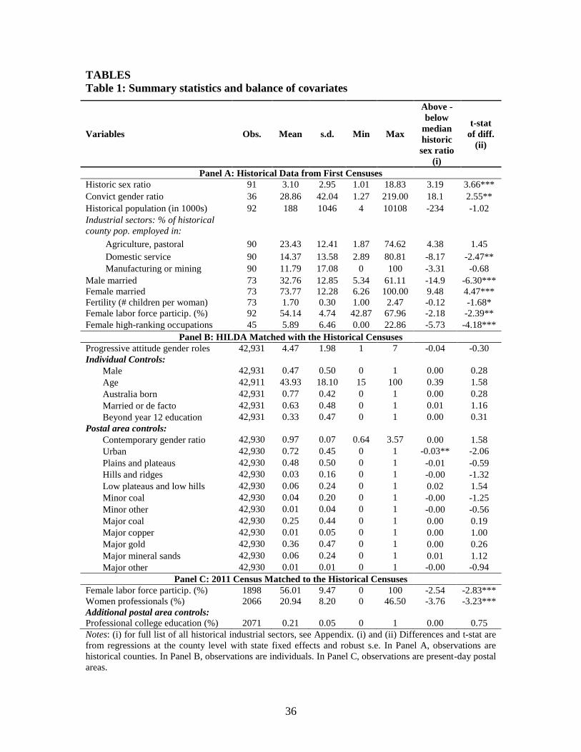
36

TABLES

Table 1: Summary statistics and balance of covariates

Variables Obs. Mean s.d. Min Max

Above -

below

median

historic

sex ratio

(i)

t-stat

of diff.

(ii)

Panel A: Historical Data from First Censuses

Historic sex ratio 91 3.10 2.95 1.01 18.83 3.19 3.66***

Convict gender ratio 36 28.86 42.04 1.27 219.00 18.1 2.55**

Historical population (in 1000s) 92 188 1046 4 10108 -234 -1.02

Industrial sectors: % of historical

county pop. employed in:

· Agriculture, pastoral 90 23.43 12.41 1.87 74.62 4.38 1.45

· Domestic service 90 14.37 13.58 2.89 80.81 -8.17 -2.47**

· Manufacturing or mining 90 11.79 17.08 0 100 -3.31 -0.68

Male married 73 32.76 12.85 5.34 61.11 -14.9 -6.30***

Female married 73 73.77 12.28 6.26 100.00 9.48 4.47***

Fertility (# children per woman) 73 1.70 0.30 1.00 2.47 -0.12 -1.68*

Female labor force particip. (%) 92 54.14 4.74 42.87 67.96 -2.18 -2.39**

Female high-ranking occupations 45 5.89 6.46 0.00 22.86 -5.73 -4.18***

Panel B: HILDA Matched with the Historical Censuses

Progressive attitude gender roles 42,931 4.47 1.98 1 7 -0.04 -0.30

Individual Controls:

Male 42,931 0.47 0.50 0 1 0.00 0.28

Age 42,911 43.93 18.10 15 100 0.39 1.58

Australia born 42,931 0.77 0.42 0 1 0.00 0.28

Married or de facto 42,931 0.63 0.48 0 1 0.01 1.16

Beyond year 12 education 42,931 0.33 0.47 0 1 0.00 0.31

Postal area controls:

Contemporary gender ratio 42,930 0.97 0.07 0.64 3.57 0.00 1.58

Urban 42,930 0.72 0.45 0 1 -0.03** -2.06

Plains and plateaus 42,930 0.48 0.50 0 1 -0.01 -0.59

Hills and ridges 42,930 0.03 0.16 0 1 -0.00 -1.32

Low plateaus and low hills 42,930 0.06 0.24 0 1 0.02 1.54

Minor coal 42,930 0.04 0.20 0 1 -0.00 -1.25

Minor other 42,930 0.01 0.04 0 1 -0.00 -0.56

Major coal 42,930 0.25 0.44 0 1 0.00 0.19

Major copper 42,930 0.01 0.05 0 1 0.00 1.00

Major gold 42,930 0.36 0.47 0 1 0.00 0.26

Major mineral sands 42,930 0.06 0.24 0 1 0.01 1.12

Major other 42,930 0.01 0.01 0 1 -0.00 -0.94

Panel C: 2011 Census Matched to the Historical Censuses

Female labor force particip. (%) 1898 56.01 9.47 0 100 -2.54 -2.83***

Women professionals (%) 2066 20.94 8.20 0 46.50 -3.76 -3.23***

Additional postal area controls:

Professional college education (%) 2071 0.21 0.05 0 1 0.00 0.75

Notes: (i) for full list of all historical industrial sectors, see Appendix. (i) and (ii) Differences and t-stat are

from regressions at the county level with state fixed effects and robust s.e. In Panel A, observations are

historical counties. In Panel B, observations are individuals. In Panel C, observations are present-day postal

areas.

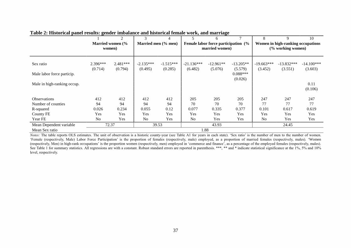
37

Table 2: Historical panel results: gender imbalance and historical female work, and marriage 1 2 3 4 5 6 7 8 9 10

Married women (%

women)

Married men (% men) Female labor force participation (%

married women)

Women in high-ranking occupations

(% working women)

Sex ratio 2.396*** 2.481*** -2.135*** -1.515*** -21.136*** -12.961** -13.205** -19.663*** -13.832*** -14.100***

(0.714) (0.794) (0.495) (0.285) (6.482) (5.076) (5.579) (3.452) (3.551) (3.603)

Male labor force particip. 0.088***

(0.026)

Male in high-ranking occup. 0.11

(0.106)

Observations 412 412 412 412 205 205 205 247 247 247

Number of counties 94 94 94 94 70 70 70 77 77 77

R-squared 0.026 0.234 0.055 0.12 0.077 0.335 0.377 0.101 0.617 0.619

County FE Yes Yes Yes Yes Yes Yes Yes Yes Yes Yes

Year FE No Yes No Yes No Yes Yes No Yes Yes

Mean Dependent variable 72.37 39.53 43.93 24.45

Mean Sex ratio 1.88

Notes: The table reports OLS estimates. The unit of observation is a historic county-year (see Table A1 for years in each state). ‘Sex ratio’ is the number of men to the number of women.

‘Female (respectively, Male) Labor Force Participation’ is the proportion of females (respectively, male) employed, as a proportion of married females (respectively, males). ‘Women

(respectively, Men) in high-rank occupations’ is the proportion women (respectively, men) employed in ‘commerce and finance’, as a percentage of the employed females (respectively, males).

See Table 1 for summary statistics. All regressions are with a constant. Robust standard errors are reported in parenthesis. ***, ** and * indicate statistical significance at the 1%, 5% and 10%

level, respectively.

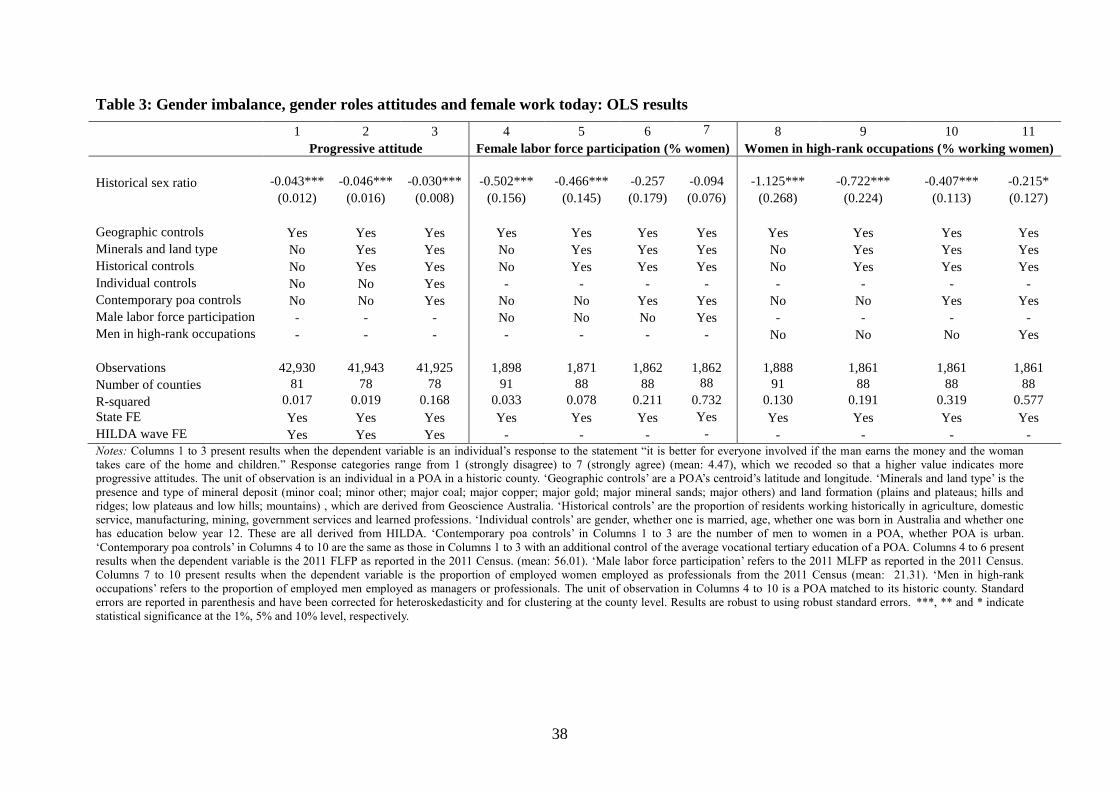
38

Table 3: Gender imbalance, gender roles attitudes and female work today: OLS results

1 2 3 4 5 6 7 8 9 10 11

Progressive attitude Female labor force participation (% women) Women in high-rank occupations (% working women)

Historical sex ratio -0.043*** -0.046*** -0.030*** -0.502*** -0.466*** -0.257 -0.094 -1.125*** -0.722*** -0.407*** -0.215*

(0.012) (0.016) (0.008) (0.156) (0.145) (0.179) (0.076) (0.268) (0.224) (0.113) (0.127)

Geographic controls Yes Yes Yes Yes Yes Yes Yes Yes Yes Yes Yes

Minerals and land type No Yes Yes No Yes Yes Yes No Yes Yes Yes

Historical controls No Yes Yes No Yes Yes Yes No Yes Yes Yes

Individual controls No No Yes - - - - - - - -

Contemporary poa controls No No Yes No No Yes Yes No No Yes Yes

Male labor force participation - - - No No No Yes - - - -

Men in high-rank occupations - - - - - - - No No No Yes

Observations 42,930 41,943 41,925 1,898 1,871 1,862 1,862 1,888 1,861 1,861 1,861

Number of counties 81 78 78 91 88 88 88 91 88 88 88

R-squared 0.017 0.019 0.168 0.033 0.078 0.211 0.732 0.130 0.191 0.319 0.577

State FE Yes Yes Yes Yes Yes Yes Yes Yes Yes Yes Yes

HILDA wave FE Yes Yes Yes - - - - - - - -

Notes: Columns 1 to 3 present results when the dependent variable is an individual’s response to the statement “it is better for everyone involved if the man earns the money and the woman

takes care of the home and children.” Response categories range from 1 (strongly disagree) to 7 (strongly agree) (mean: 4.47), which we recoded so that a higher value indicates more

progressive attitudes. The unit of observation is an individual in a POA in a historic county. ‘Geographic controls’ are a POA’s centroid’s latitude and longitude. ‘Minerals and land type’ is the

presence and type of mineral deposit (minor coal; minor other; major coal; major copper; major gold; major mineral sands; major others) and land formation (plains and plateaus; hills and

ridges; low plateaus and low hills; mountains) , which are derived from Geoscience Australia. ‘Historical controls’ are the proportion of residents working historically in agriculture, domestic

service, manufacturing, mining, government services and learned professions. ‘Individual controls’ are gender, whether one is married, age, whether one was born in Australia and whether one

has education below year 12. These are all derived from HILDA. ‘Contemporary poa controls’ in Columns 1 to 3 are the number of men to women in a POA, whether POA is urban.

‘Contemporary poa controls’ in Columns 4 to 10 are the same as those in Columns 1 to 3 with an additional control of the average vocational tertiary education of a POA. Columns 4 to 6 present

results when the dependent variable is the 2011 FLFP as reported in the 2011 Census. (mean: 56.01). ‘Male labor force participation’ refers to the 2011 MLFP as reported in the 2011 Census.

Columns 7 to 10 present results when the dependent variable is the proportion of employed women employed as professionals from the 2011 Census (mean: 21.31). ‘Men in high-rank

occupations’ refers to the proportion of employed men employed as managers or professionals. The unit of observation in Columns 4 to 10 is a POA matched to its historic county. Standard

errors are reported in parenthesis and have been corrected for heteroskedasticity and for clustering at the county level. Results are robust to using robust standard errors. ***, ** and * indicate statistical significance at the 1%, 5% and 10% level, respectively.

39

Table 4: Gender imbalance and attitudes and female work today: IV results

1 2

Progressive attitude Women in high-rank

occupations

Panel A: Second Stage IV estimation results

Historical sex ratio -0.206*** -0.564*

-0.077 -0.341

Geographic controls Yes Yes

Minerals and land type Yes Yes

Historical controls Yes Yes

Individual controls Yes -

Contemporary poa controls Yes Yes

Number of convicts Yes Yes

Men in high-rank occupations - Yes

Observations 13,847 483

Number of counties 28 31

R-squared 0.165 0.802

State FE Yes Yes

HILDA wave FE Yes -

Panel B: First stage estimation results

Convict sex ratio 0.027** 0.033***

-0.01 -0.006

Observations 13,847 483

Number of counties 28 31

F statistic 7.03 27.62

Adjusted R-squared 0.911 0.876

Notes: See Table 4 for the list of controls. The table reports 2SLS estimates. All the controls are identical to those included

in Table 4 and are identical in the first and second stages (Panel A and B). Standard errors are reported in parenthesis and

have been corrected for heteroskedasticity and for clustering at the county level.

40

Table 5: Persistence: vertical cultural transmission by fathers and homogamy

1 2 3 4 5 6 7 8 9 10

Dependent variable: Progressive attitude

All areas Low migration High migration High Homogamy Low Homogamy

Historical sex ratio -0.017 0.019 -0.023*** 0.007 0.418 0.456 -0.030** 0.007 -0.079 -0.109

(0.017) (0.013) (0.007) (0.013) (0.279) (0.289) (0.008) (0.014) (0.189) (0.187)

Australian father 0.340*** 0.213*** 0.113 0.301*** 0.136* 0.271***

(0.066) (0.056) (0.071) (0.077) (0.090) (0.076)

Australian father * sex ratio -0.093*** -0.077*** -0.037** -0.064 -0.046** -0.045

(0.035) (0.022) (0.017) (0.038) (0.019) (0.030)

Australian mother -0.013 0.065

(0.068) (0.054)

Australian mother * sex ratio 0.047* 0.014

(0.027) (0.019)

Geographic controls Yes Yes Yes Yes Yes Yes Yes Yes Yes Yes

Minerals and land type Yes Yes Yes Yes Yes Yes Yes Yes Yes Yes

Historical controls Yes Yes Yes Yes Yes Yes Yes Yes Yes Yes

Individual controls No Yes Yes Yes Yes Yes Yes Yes Yes Yes

Contemporary poa controls No Yes Yes Yes Yes Yes Yes Yes Yes Yes

Yes Yes

Observations 41,943 41,925 20,971 20,971 20,954 20,954 20,490 20,490 21,438 21,438

R-squared 0.026 0.169 0.166 0.167 0.175 0.176 0.170 0.170 0.171 0.173

State FE Yes Yes Yes Yes Yes Yes Yes Yes Yes Yes

HILDA wave FE Yes Yes Yes Yes Yes Yes Yes Yes Yes Yes

Notes: See Table 4 for the list of controls. ‘Low migration’ refers to POAs where the proportion of residents born in Australia is higher than the median proportion of residents

born in Australia as per the 2011 Census. ‘High migration’ refers to POAs where the proportion of residents born in Australia is lower than the median proportion of residents born

in Australia as per the 2011 Census. Homogamy refers to the average proportion of people of Australian decent in the POA who married someone also of Australian decent. ‘Low

Homogamy’ are postal areas to POAs whose predicted level of homogamy lies below the median level of homogamy, which is 85%. ‘High Homogamy’ refers to POAs whose

predicted level of homogamy lies above the median. Homogamy is predicted by the sex ratio today, the degree of urbanisation, income, education, shares of employment in 18

different industries and respondents’ parents’ countries of birth in the postal area Standard errors are reported in parenthesis and have been corrected for heteroskedasticity and for

clustering at the county level.

41

Table 6: Welfare implications: income, satisfaction, and time use

1 2 3 4 5 6 7

Log annual income Satisfied with partner Time spent each week in:

Care of children

Historical sex ratio -0.018* -0.006 0.000 0.039*** 0.019* 0.003 -0.017

(0.010) (0.010) (0.007) (0.010) (0.011) (0.075) (0.067)

Female -0.430*** -0.414*** -0.210 -0.245*** -0.251*** 4.603*** 4.834***

(0.043) (0.040) (0.144) (0.029) (0.031) (0.202) (0.230)

Female * Historical sex ratio -0.029* -0.030** -0.023** 0.001 0.004 -0.155* -0.186**

(0.016) (0.015) (0.011) (0.012) (0.011) (0.078) (0.083)

Geographic controls Yes Yes Yes Yes Yes Yes Yes

Extended geographic controls No Yes Yes No Yes No Yes

Historical controls No Yes Yes No Yes No Yes

Contemporary poa controls No Yes Yes No Yes No Yes

Individual controls No Yes Yes No Yes No Yes

Family structure controls - - - - No Yes

Occupation-gender dummies No No Yes - - - -

Industry-gender dummies No No Yes - - - -

Observations 20,285 19,852 19,740 31,282 30,512 38,535 37,641

R-squared 0.096 0.176 0.306 0.009 0.047 0.024 0.229

State FE Yes Yes Yes Yes Yes Yes Yes

HILDA wave FE Yes Yes Yes Yes Yes Yes Yes

Notes: The level of observation is an individual. ‘Geographic controls’, ‘Minerals and land type’, ‘Historical controls’, ‘Contemporary poa controls’ and ‘Individual controls’ are

as in Table 4. The dependent variable in Columns 1 to 3 is the log of individual gross wages and salary. ‘Occupation dummies’: Managers; Professionals; Technician and trade

workers; Community and personal service workers; Clerical and administrative workers; Sales workers; Machinery operators and drivers; Laborers. ‘Industry dummies’:

Agriculture, forestry, fishing; Mining; Manufacturing; Electricity, gas, water, waste; Construction; Wholesale trade; Retail trade; Accommodation and food; Transport, postal and

warehousing; Information, media and telecommunications; Financial and insurance; Real estate; Professional, scientific and technical; Public administration and safety; Education

and training; Health care and social; Arts and recreation; Other services. Occupation- and Industry-gender dummies are the full list of, respectively, occupation and industry

dummies interacted with female. The dependent variable in Columns 4 and 5 is individual responses to the question “how satisfied are you with your relationship with your

partner?” Response categories range from 0 (completely dissatisfied) to 10 (completely satisfied). ‘Family structure’ indicates the number of young children (under the age of 15)

and the number of dependent children. Standard errors are reported in parenthesis and have been corrected for heteroskedasticity and for clustering at the county level.

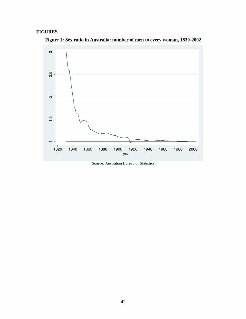
42

FIGURES

Figure 1: Sex ratio in Australia: number of men to every woman, 1830-2002

Source: Australian Bureau of Statistics

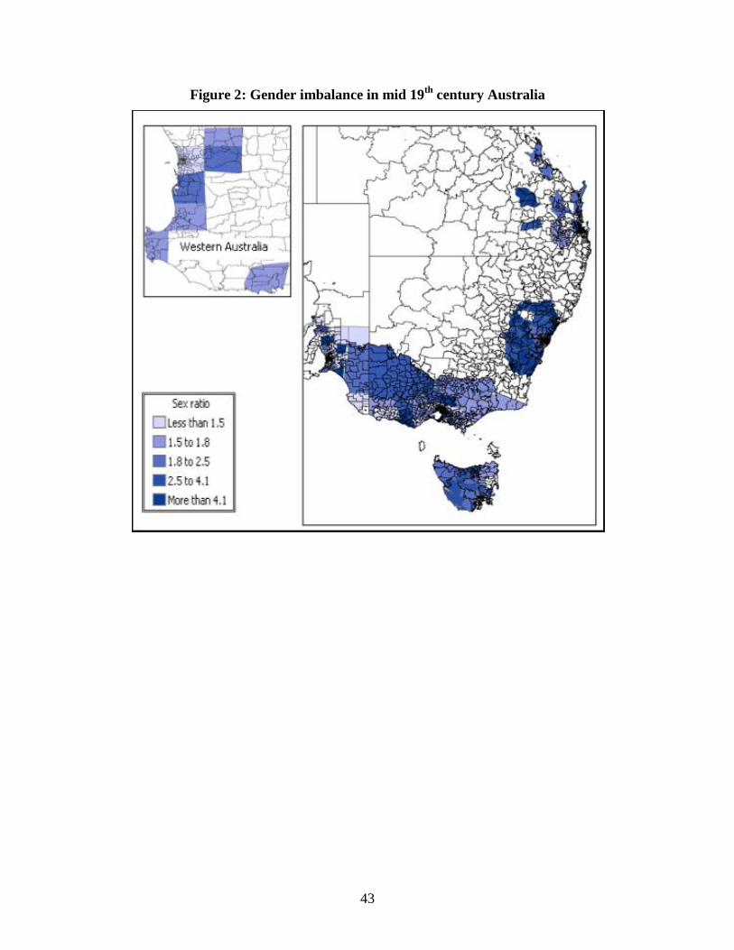
43

Figure 2: Gender imbalance in mid 19th

century Australia

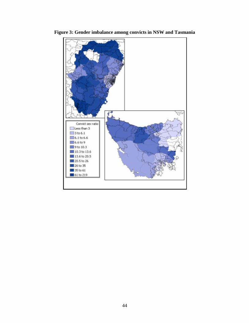
44

Figure 3: Gender imbalance among convicts in NSW and Tasmania