JACOBSTHAL AND PELL CURVES

A. Fe HORADAM University of New England, Armidale, NSW, 2351, Australia

(Submitted August 1986)

1. INTRODUCTION

In an earlier paper [2], a study was made of Fibonacci and Lucas curves in

the plane, and their Laser-printed graphs were exhibited. These graphs were

drawn from the equations of the curves, rather than from the tabulated lists

of values of the Cartesian coordinates x and y9 which also served a purpose of

their own. It is desirable to extend the work in [2] and so produce a more

complete theory.

Here, we present basic information about the corresponding curves associ-

ated with (i) Pell and Pell-Lucas numbers, and (11) Jacobsthal and Jacobs thai-Lucas numbers, in our nomenclature.

Curves associated with (i) will carry the generic name of Pell curves while

those connected with (ii) will be designated Jacobsthal curves, There seems to

be no theory related to (i) and (ii) which corresponds to the result of Halsey

[1] for Fibonacci numbers.

To avoid unnecessary duplication in our discussion, we will consider the

numbers in (i) and (ii) (as well as the Fibonacci and Lucas numbers) to be spe-

cial instances of a general sequence {wn} whose relevant properties will be investigated.

Thus, the Pell and Jacobsthal curves, as well as the Fibonacci and Lucas

curves, may be thought of as members of a family of curves which we shall des-

ignate as w-curves. The two Pell curves and the two Jacobsthal curves resemble the Fibonacci

and Lucas curvess so we will not reproduce them here* Instead, the reader is

invited to compare them in the mind?s eye with the curves exhibited in [2].

2a GENERALITIES

Let a, b, p, and q be real numbers, usually integers. Define the sequence {wn} by

Wn+2 = PWn + l ~ ^n* W0 = 2 b > Wl = a + & (n > 0) B (2.1)

1988] 77

JACOBSTHAL AND PELL CURVES

Extension to negative values of n may be made, but we do not require it here.

The explicit Binet form for Wn is

wn = (Aan - S3n)/(a - B),

where a, B are the roots of the characteristic equation

X2 - pX + q = 0,

so t h a t

and

a = (p + Vp2 - 4<?)/2 = (p - Vp2 - 4qr)/2

^ a + B = p , a 6 = ^ 5 a B = v^2 - 4q

The Fibonacci and Lucas sequences are well known.

Some values for the other sequences are:

{Qn}

{J J {«/„}

In what follows, q < 0.

Write

<? = -1 • 2> (r > 0) ,

so, by (2.4)

n = 0

0

2

0

2

1

1

2

1

1

2

2

6

1

5

3

5

14

3

7

4

12

34

5

17

5

29

82

11

31

6

70

198

21

65

7

169

478

43

127 . . .

3 = -1

Only the cases

q = -1,

78

a

i.e., r = 1 [cf. (2.5)-(2.8)]

(2.2)

(2.3)

(2.4)

(A = a + b - 2&B, \ B = a + 6 - 26a .

S p e c i a l c a s e s of iwn]

SEQUENCE

{Fn}: F i b o n a c c i

{Z/n}: Lucas

{ P n } : P e l l

{ $ n } : P e l l - L u c a s

{ j n } : J a c o b s t h a l

a r e :

{jn}:Jacobsthal-Lucas

P

1

1

2

2

1

1

<7

- 1

- 1

- 1

- 1

- 2

- 2

a

1

0

1

1

1

0

b

0

1

0

1

0

1

a

(1 + i / 5 ) /2

(1 + i /5 ) /2

1 + 1/2

1 + yfl

2

2

(1

(1 1

1

g

- i/5)/2 - V5)/2 - / 2

- / 2

- 1

- 1

( 2 . 5 )

( 2 . 5 )

( 2 . 6 )

( 2 . 7 )

( 2 . 8 )

( 2 . 9 )

( 2 . 1 0 )

(2.11)

(2.12)

(2.13)

(2.14)

(2.15)

(2.16)

(2.17)

[Feb.

JACOBSTHAL AND PELL CURVES

and

3 = -1, i.e., v = a (= 2) [cf. (2.9)-(2.10)]

will concern us.

3. THE w-CURVES

For Cartesian coordintes xs y of a point in the plane, let

x = ^ c t 0 - B(~) COS 0TrV(a - 3)

and

( 2 . 1 8 )

( 3 . 1 )

( 3 . 2 ) y = -£oT b s i n 9Tr/(a - 6 ) ,

where 0 i s r e a l , ,

Comparing ( 3 . 1 ) w i t h ( 2 . 2 ) 5 we may r e f e r t o ( 3 , 1 ) a s t h e genevdl'Lzed B-Lnet

form of wn* When 0 = n , i n t e g e r , we have x = Wn by ( 2 . 2 ) and ( 3 . 1 ) .

As 0 v a r i e s i n ( 3 . 1 ) and ( 3 . 2 ) , we o b t a i n t h e W-curves.

Now, from ( 3 . 1 ) and ( 3 . 2 ) , we have

and

dy de dx

Ba~Q ( l o g a s i n OTT - TT COS 0f r ) / ( a - 3)

l o g a + 5 ^ ) " 0 | l o g ^ c o s 0TT + IT s i n 0TT| /(a - 3) ,

whence -f- = 0 i f dx

t a n 0TT = ( 6 . 5 2 8 f o r ( 2 . 5 ) , ( 2 . 6 ) — s e e [2]

= < 3 . 5 6 5 f o r ( 2 . 7 ) , ( 2 . 8 ) ( 4 . 5 3 8 f o r ( 2 . 9 ) , ( 2 . 1 0 ) log a

yielding

07T = 8 1 ° 1 6 f , 7 4 ° 2 1 f , 7 7 ° 3 4 f ,

r e s p e c t i v e l y , i . e . ,

( 0 . 4 5 0 = < 0 . 4 1

1 0 . 4 3 ,

respectively, for the three cases in (3.5).

Write (3.5) as

{si (CO

i n QTI = ±ki\ cos Qn = ±k l o g a ,

i . e . ,

g i v i n g

k = [TT2 + ( l o g a ) 2 ] ~ 1 / 2

( 0 . 3 1 k = < 0 . 3 0

( 0 . 2 9 9 ,

respectively, for the three, cases in (3.5).

(3.3)

(3.4)

(3.5)

(3.6)

(3.7)

(3.8)

(3.8)'

1988] 79

JACOBSTHAL AND PELL CURVES

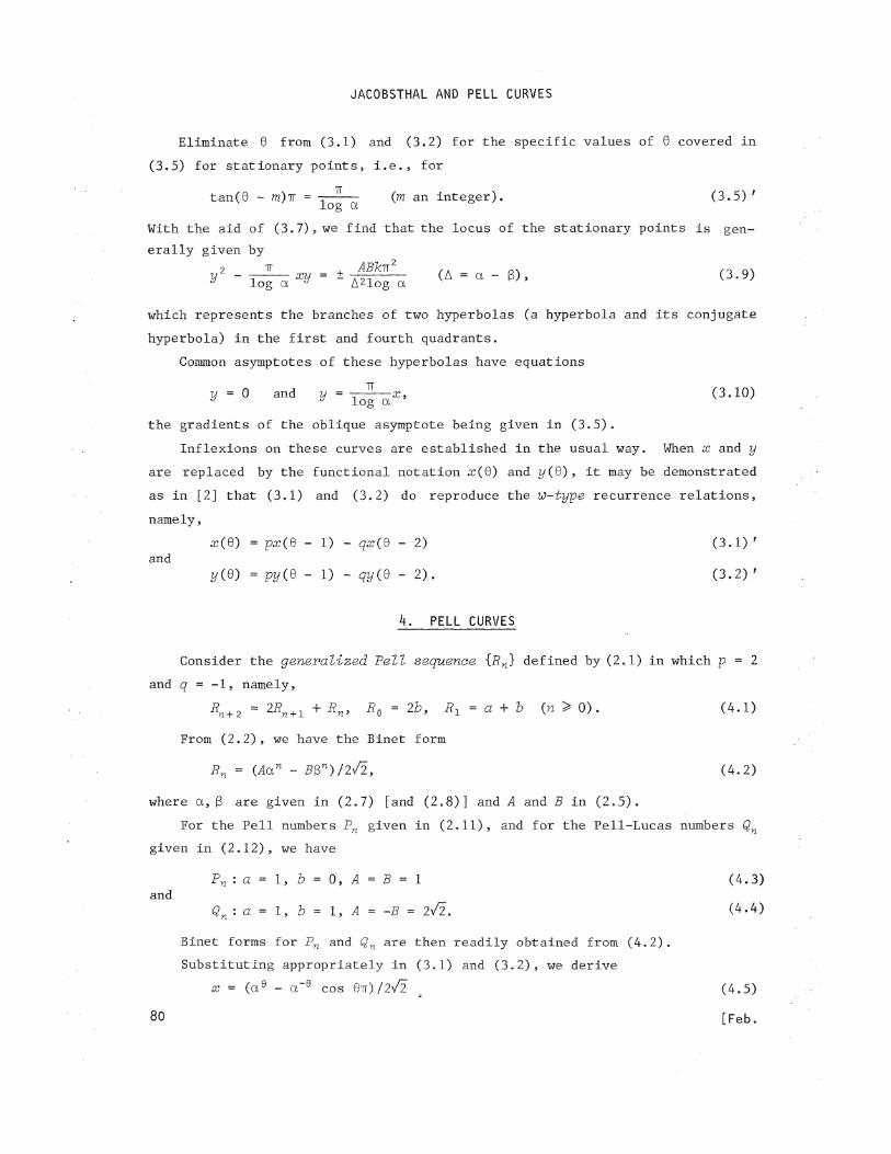
Eliminate 0 from (3.1) and (3.2) for the specific values of 0 covered in

(3.5) for stationary points.* i.e., for

tan(0 - m)TT = — (m an integer). (3.5) f

With the aid of (3.7) , we find that the locus of the stationary points is gen-

erally given by

y2 - TJL—xy = ± ^ — ( A = a - g ) , (3,9)

y log a ^ A2log a

which represents the branches of two hyperbolas (a hyperbola and its conjugate

hyperbola) in the first and fourth quadrants.

Common asymptotes of these hyperbolas have equations

y = 0 and y = — — — x 9 (3.10) y v log a

the gradients of the oblique asymptote being given in (3.5). Inflexions on these curves are established in the usual way. When x and y

are replaced by the functional notation x(Q) and z/(0), it may be demonstrated

as in [2] that (3.1) and (3.2) do reproduce the w-type recurrence relations,

namely,

x(0) = px(Q - 1) - qx(Q - 2) (3.1) r

and z/(9) = py(Q - 1) - qy(Q - 2) . (3.2)'

h. PELL CURVES

Consider the generalized Fell sequence {Rn} defined by (2.1) in which p = 2

and q = -1, namely, Rn+2 = 2Rn + l + Rn> R0 = 2b> Rl = a + b (n > ° >• (4-1>

From (2,2), we have the Binet form

Rn = (Aan - B$n)/2/2s (4.2)

where a, (3 are given in (2.7) [and (2.8)] and A and B in (2.5). For the Pell numbers Pn given in (2.11), and for the Pell-Lucas numbers Qn

given in (2.12), we have

Pn : a = 1, b = 0, A = B = 1 (4.3) and

Qn : a = 1, b = 1, A = -B = 2^2. (4.4)

Binet forms for Pn and S n are then readily obtained from (4.2).

Substituting appropriately in (3.1) and (3.2), we derive

x = ( a e - a" e cos 9TT)/2V/2 4 ( 4 . 5 )

80 [Feb.

JACOBSTHAL AND PELL CURVES

and y = _ a " 0 s i n 0TF/2V^ ( 4 . 6 )

f o r t h e P e l l c a s e s and

x = a 6 + a"e cos 9TT ( 4 . 7 ) and

y = a"6 s i n 0TT ( 4 . 8 )

for the Pell-Lucas case.

Equations (4,5) and (4.7) are the modified Binet forms for Pn and Qn, re-spectively. When 0 = n9 integer, we get the usual Binet forms for Pn and Qn, ise*3 x = Pn and x = Qn9 respectively*

The locus given by (4.5) and (4.6) is the Pell curve. Its stationary points

lie on the two appropriate branches of the hyperbolas

y2 - i- 5— xy = ± —^—- (a = 1 + V2). (4.9) J log a y 8 log a v v '

Equations (4.7) and (4.8) yield the Pell-Lucas curve. Stationary points of

this curve lie on the hyperbolic curves

yz _ —2—xy = ± J 2 ! _ (a = i + ^2). (4.10) ^ log a -7 log a

In both (4.9) and (4.10), the value of k is given in (3.8) f. Asymptotes

common to the curves in (4.9) and (4.10) are y = 0 and y = (ir/log a)#, whose gradient is given in (3.5).

Suppose we put a = 3̂ b = 1 in (4.1) so that ,4 = 2a, 5 = 2$9 Then (4.1) or the Binet forms for Pn$ Qn9 and Rn yield

P* = 2Pn +.Qn (4.11)

= 2Pn+1 since Qn = Pn+1 + Pn_1.

Thus, a composite curve for 2P6 + Qs is equivalent to the Pell curve for 2PQ + 1.

Furthermore, from (4.11) or the Binet forms, we deduce that

Rn = (a - &)Pn + W „ (4.12)

= (a-£)P„ + M P n + 1 +P„. 1)

= (a + 2>)P„ + 2£P n v n n -1

[= P* = 2P _,., when a = 3, & = 1, as in (4.11)]. n n +1

5, JACOBSTHAL CURVES

Next3 consider the generalized Jacobsthal sequence i^n} given by

A + 2 = A + i + 2/n> / o " 2 6 » /ima + b &><>). (5.1) 1988] 81

JACOBSTHAL AND PELL CURVES

From (2,2), we have the Binet form

A = ^ m i (5.2)

in which a (= 2), S (= -1) are already given in (2.9) and (2.10), and A, B are given in (2.5).

Particular cases of (5.1) are the Jacobsthal numbers Jn given in (2.13) and

the Jacobsthal-Lucas numbers j n given in (2.14) for which

Jn i a = 1, b = 0, A = B = 1 (5.3) and

j n : a = 0, b = 1, A = -B = 3. (5.4)

Binet forms for Jn and j n then readily follow from (5.2).

Appropriate substitution in (3.1) and (3.2) produces

x = (2e - cos 9TT)/3 (5.5) and

y = -2"e sin QTT/3 (5.6)

for Jn 5 and

x = 2e + cos 9TT (5.7) and

y = 2"e sin 0TT (5.8)

for j n . Note the effect of (2.18) on (3.1) in (5.5) and (5.7).

Equations (5.5) and (5.7) are the modified Binet forms for Jn and j n 9 re-

spectively. Setting G = ns integer, we have the ordinary Binet forms for Jn

and j„, i.e.5 x - Jn and x - j n 9 respectively.

The locus given by (5.5) and (5.6) is the Jacobsthal curve. Its stationary

points lie on the appropriate branches of the rectangular hyperbolas

y (x±iLl|^) = T * E . (5.9)

Equations (5.7) and (5.8) yield the Jacobs thai-Lucas curve. Its stationary

points lie on the rectangular hyperbolic branches

y(x ± k log 2) = +fe7T. (5.10)

In both (5.9) and (5.10), the value of k is given in (3.8) '. Put a = 1, b = 1 in (5.1) so that A = -B = 4. Hence, as for the Pell case,

Jn = Jn + Jn (5.11) = 2J Mn.

n + 1

82 [Feb.

JACOBSTHAL AND PELL CURVES

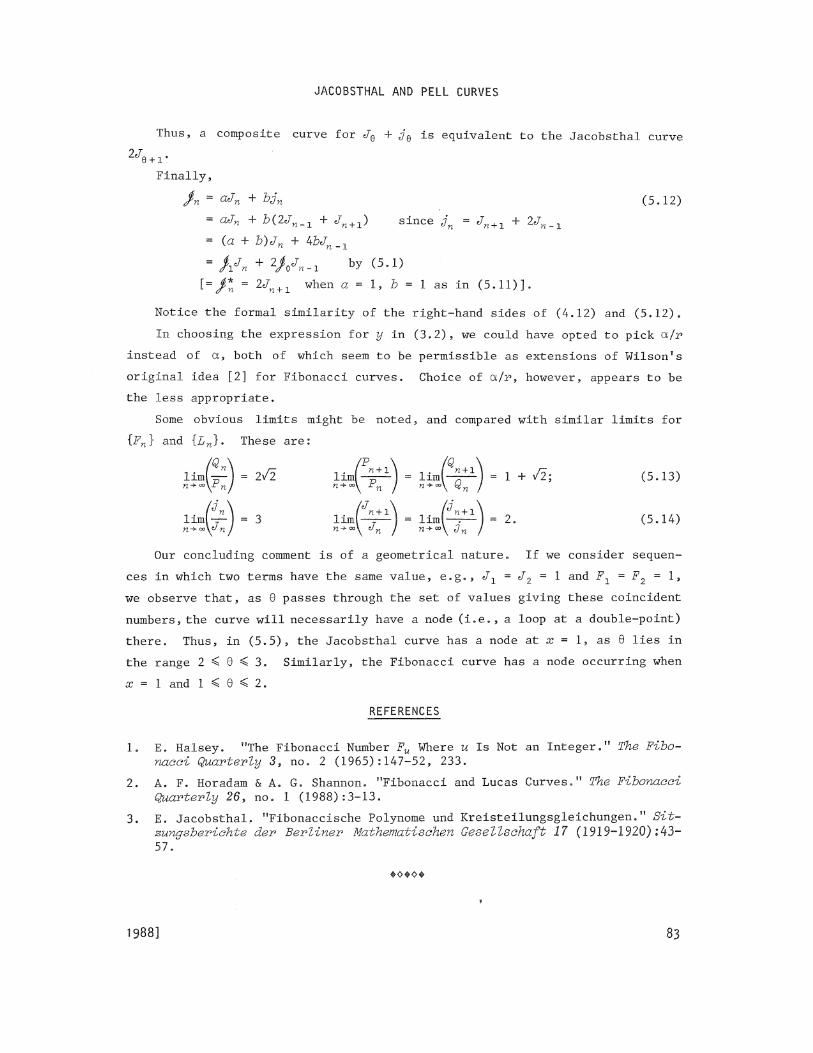
Thus, a composite curve for JQ + j Q is equivalent to the Jacobsthal curve

Finallys

A = aJn + bJn (5.12)

= aJn + b{2Jn_1 + Jn + 1) since j n = Jn + 1 + 2Jn_±

= (a + b)Jn + tt>Jn_x

= AJn + 2M-1 b^ (5 >̂ [=/* = 2Jn + 1 when a = 1, 2? = 1 as in (5.11)].

Notice the formal similarity of the right-hand sides of (4,12) and (5.12).

In choosing the expression for y in (3.2), we could have opted to pick a/r

instead of a, both of which seem to be permissible as extensions of Wilson1s

original idea [2] for Fibonacci curves. Choice of a/r, however, appears to be

the less appropriate.

Some obvious limits might be noted, and compared with similar limits for

{Fn} and {Ln}B These are:

liml-y-J = 3 liml—-— = liml—:—-

Our concluding comment is of a geometrical nature. If we consider sequen-

ces in which two terms have the same value, e.g., J1 = J2 = 1 and F1 = F2 = 1,

we observe that, as 0 passes through the set of values giving these coincident

numbers, the curve will necessarily have a node (i.e., a loop at a double-point)

there. Thus, in (5.5), the Jacobsthal curve has a node at x = 1, as 6 lies in

the range 2 < 6 < 3. Similarly, the Fibonacci curve has a node occurring when

x = 1 and 1 < 6 < 2.

REFERENCES

1. E. Halsey. "The Fibonacci Number Fu Where u Is Not an Integer.11 The Fibo-nacci Quarterly 3S no* 2 (1965)®147-52, 233.

2. A. F. Horadam & A. G. Shannon. "Fibonacci and Lucas Curves." The Fibonacci Quarterly 26, no. 1 (1988):3-13.

3. E. Jacobsthal, "Fibonaccische Polynome und Kreisteilungsgleichungen." Sit-zungsberiohte der Berliner Mathematischen Gesellschaft 17 (1919-1920);43-~ 57.

•••<>•

= 1 + /2:

= 2.

(5.13)

(5.14)

1988] 83