j. besson centre des matériaux, École des mines de paris,...

Non linear finite element method

J. BessonCentre des Matériaux, École des Mines de Paris,

UMR CNRS 7633, BP 87 Evry cedex 91003

Non linear finite element method 1

Introduction — Outline

• The finite element method

• Application to mechanics

• Solving systems of non linear equations

• Incompressibility

Introduction 2

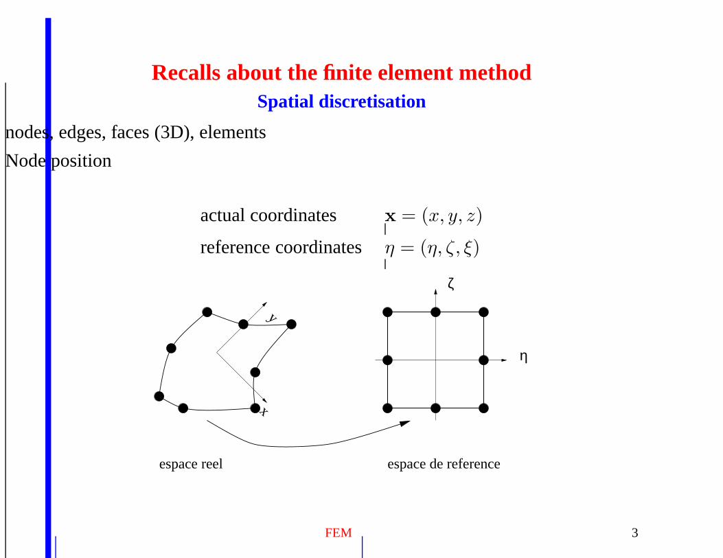
Recalls about the finite element methodSpatial discretisation

nodes, edges, faces (3D), elements

Node position

actual coordinates x = (x, y, z)

reference coordinates η = (η, ζ, ξ)

η

ζ

xy

espace reel espace de reference

FEM 3

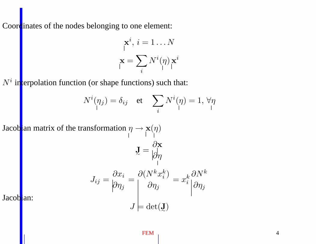
Coordinates of the nodes belonging to one element:

xi, i = 1 . . . N

x =∑

i

N i(η)xi

N i interpolation function (or shape functions) such that:

N i(ηj) = δij et∑

i

N i(η) = 1, ∀η

Jacobian matrix of the transformation η → x(η)

J∼

=∂x

∂η

Jij =∂xi

∂ηj

=∂(Nkxk

i )

∂ηj

= xki

∂Nk

∂ηj

Jacobian:J = det(J

∼)

FEM 4

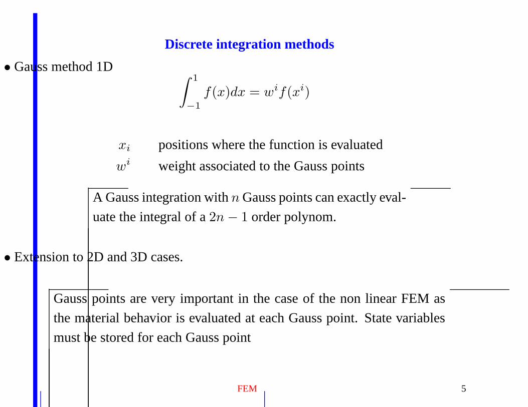
Discrete integration methods

• Gauss method 1D∫ 1

−1

f(x)dx = wif(xi)

xi positions where the function is evaluated

wi weight associated to the Gauss points

A Gauss integration with n Gauss points can exactly eval-

uate the integral of a 2n − 1 order polynom.

• Extension to 2D and 3D cases.

Gauss points are very important in the case of the non linear FEM as

the material behavior is evaluated at each Gauss point. State variables

must be stored for each Gauss point

FEM 5

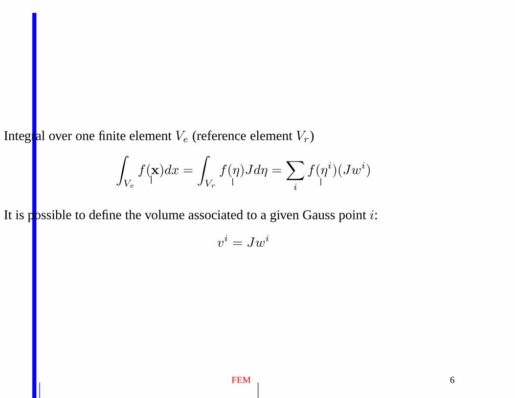
Integral over one finite element Ve (reference element Vr)∫

Ve

f(x)dx =

∫

Vr

f(η)Jdη =∑

i

f(ηi)(Jwi)

It is possible to define the volume associated to a given Gauss point i:

vi = Jwi

FEM 6

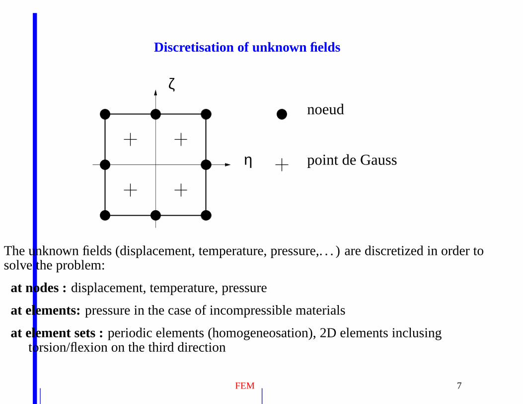
Discretisation of unknown fields

η

ζ

noeud

point de Gauss

The unknown fields (displacement, temperature, pressure,. . . ) are discretized in order tosolve the problem:

at nodes : displacement, temperature, pressure

at elements: pressure in the case of incompressible materials

at element sets : periodic elements (homogeneosation), 2D elements inclusingtorsion/flexion on the third direction

FEM 7

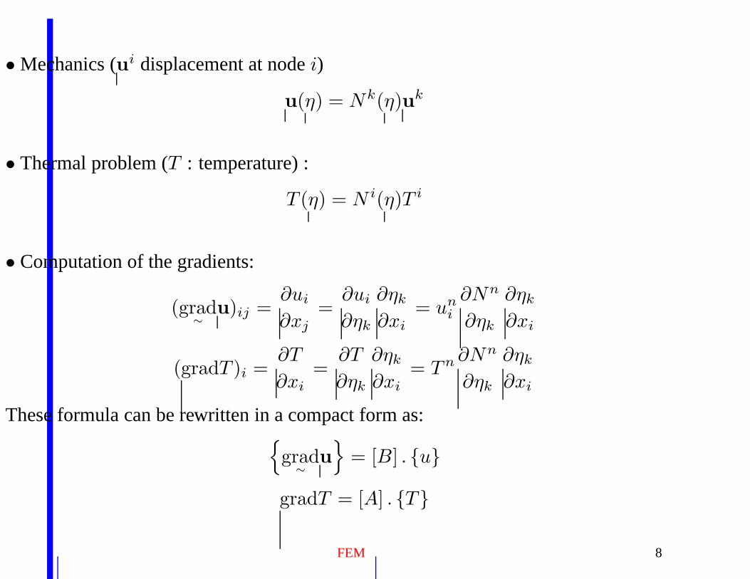
• Mechanics (ui displacement at node i)

u(η) = Nk(η)uk

• Thermal problem (T : temperature) :

T (η) = N i(η)T i

• Computation of the gradients:

(grad∼

u)ij =∂ui

∂xj

=∂ui

∂ηk

∂ηk

∂xi

= uni

∂Nn

∂ηk

∂ηk

∂xi

(gradT )i =∂T

∂xi

=∂T

∂ηk

∂ηk

∂xi

= Tn ∂Nn

∂ηk

∂ηk

∂xi

These formula can be rewritten in a compact form as:

grad∼

u

= [B] . u

gradT = [A] . T

FEM 8

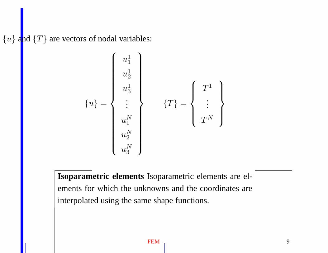
u and T are vectors of nodal variables:

u =

u11

u12

u13

...

uN1

uN2

uN3

T =

T 1

...

TN

Isoparametric elements Isoparametric elements are el-

ements for which the unknowns and the coordinates are

interpolated using the same shape functions.

FEM 9

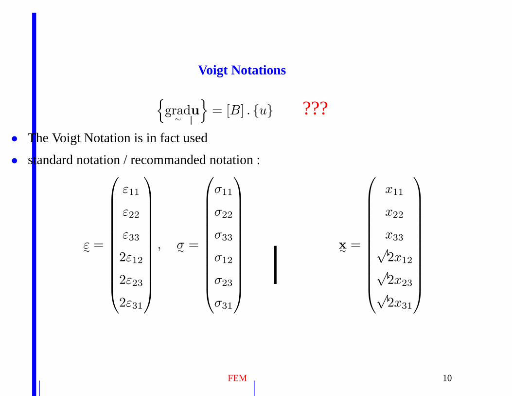
Voigt Notations

grad∼

u

= [B] . u ???

• The Voigt Notation is in fact used

• standard notation / recommanded notation :

ε∼

=

ε11

ε22

ε33

2ε12

2ε23

2ε31

, σ∼

=

σ11

σ22

σ33

σ12

σ23

σ31

x∼

=

x11

x22

x33√2x12√2x23√2x31

FEM 10

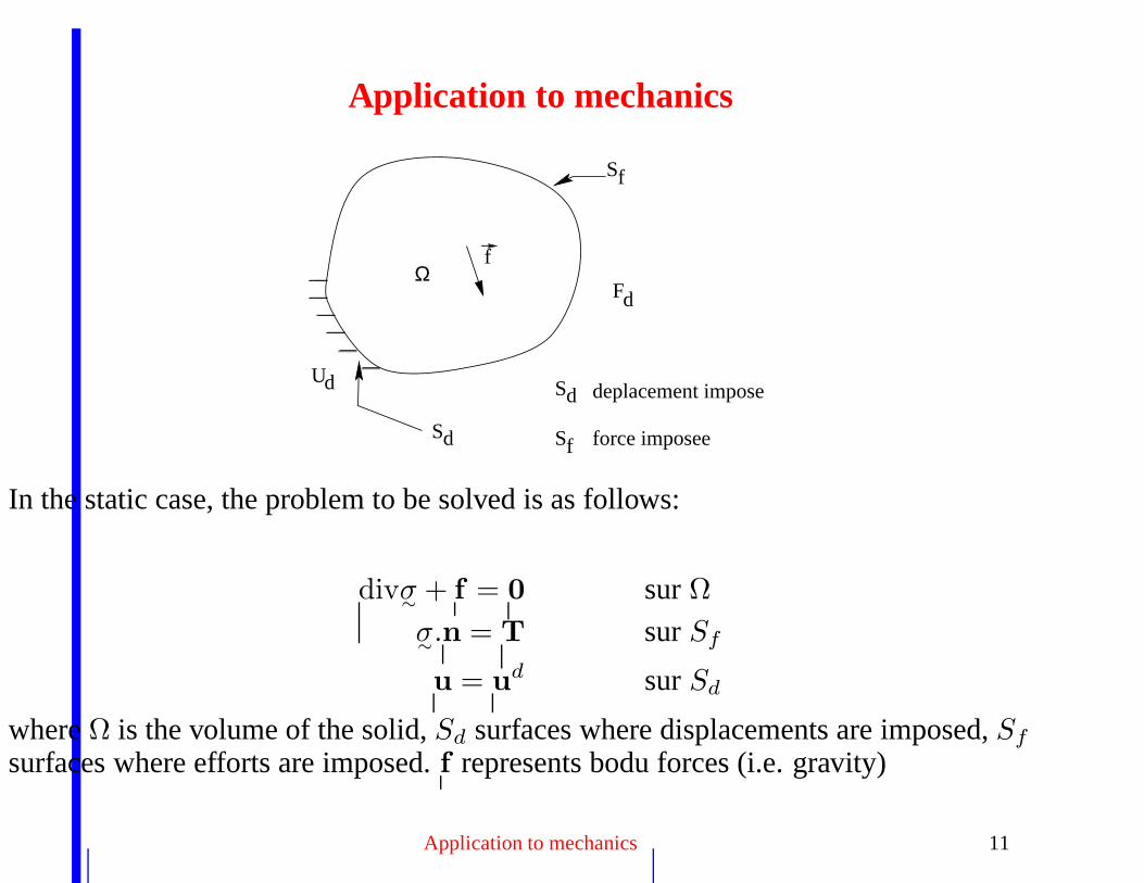
Application to mechanics

Ud

Fd

Sd

Sf

deplacement impose

force imposee

Sd

Sf

Ωf

In the static case, the problem to be solved is as follows:

divσ∼

+ f = 0 sur Ω

σ∼.n = T sur Sf

u = ud sur Sd

where Ω is the volume of the solid, Sd surfaces where displacements are imposed, Sf

surfaces where efforts are imposed. f represents bodu forces (i.e. gravity)

Application to mechanics 11

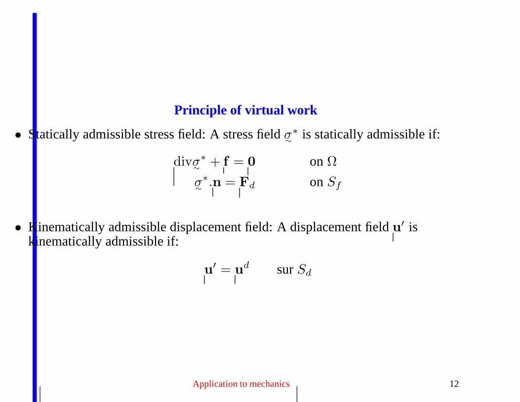
Principle of virtual work

• Statically admissible stress field: A stress field σ∼

∗ is statically admissible if:

divσ∼

∗ + f = 0 on Ω

σ∼

∗.n = Fd on Sf

• Kinematically admissible displacement field: A displacement field u′ is

kinematically admissible if:

u′ = u

d sur Sd


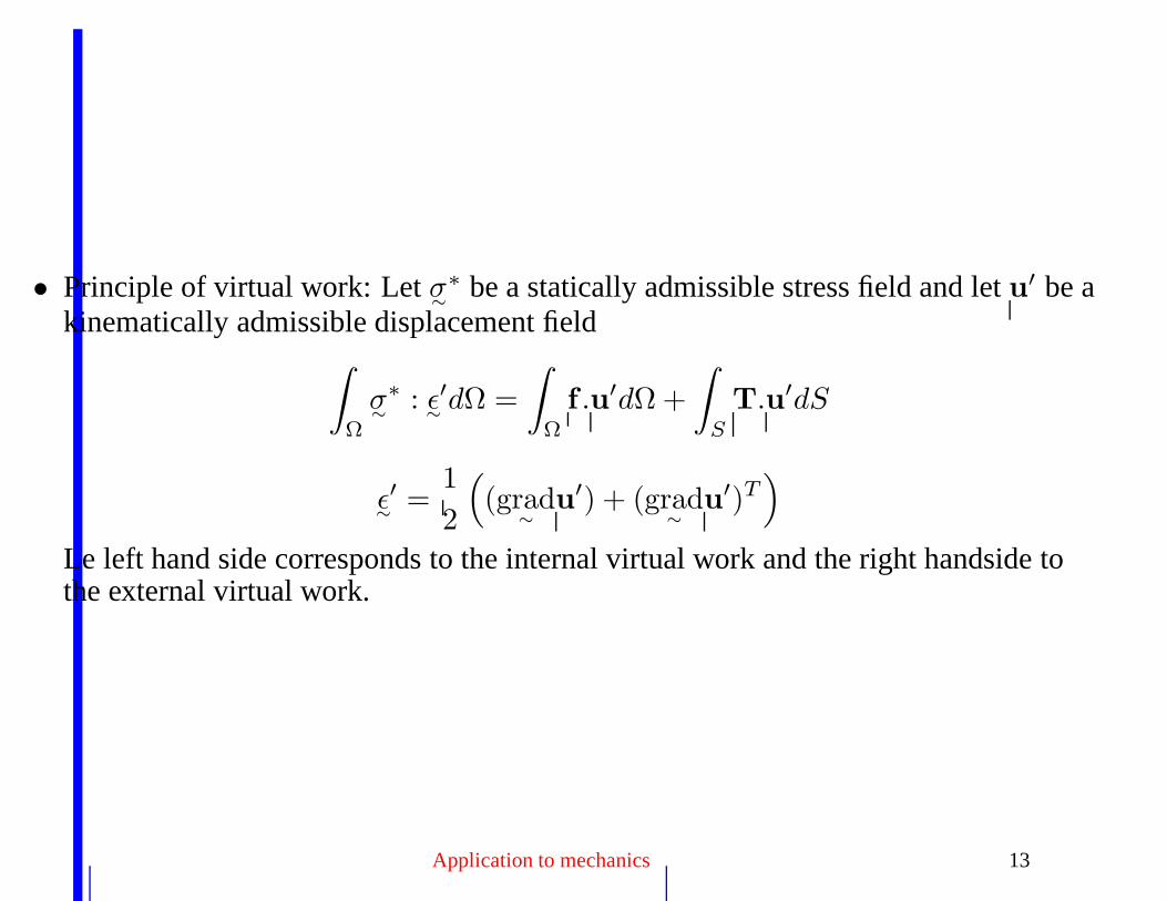
• Principle of virtual work: Let σ∼

∗ be a statically admissible stress field and let u′ be akinematically admissible displacement field

∫

Ω

σ∼

∗ : ε∼

′dΩ =

∫

Ω

f .u′dΩ +

∫

S

T.u′dS

ε∼

′ =1

2

(

(grad∼

u′) + (grad

∼

u′)T)

Le left hand side corresponds to the internal virtual work and the right handside tothe external virtual work.


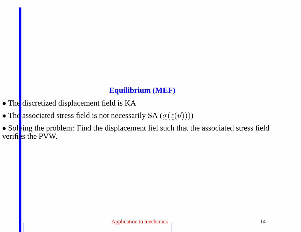
Equilibrium (MEF)

• The discretized displacement field is KA

• The associated stress field is not necessarily SA (σ∼(ε∼(~u))))

• Solving the problem: Find the displacement fiel such that the associated stress fieldverifies the PVW.


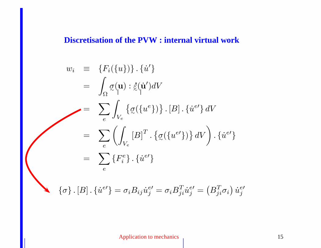
Discretisation of the PVW : internal virtual work

wi ≡ Fi(u) . u′

=

∫

Ω

σ∼(u) : ε

∼(u′)dV

=∑

e

∫

Ve

σ∼(ue)

. [B] . ue′ dV

=∑

e

(∫

Ve

[B]T

.

σ∼(ue′)

dV

)

. ue′

=∑

e

F ei . ue′

σ . [B] . ue′ = σiBij ue′j = σiB

Tjiu

e′j =

(

BTjiσi

)

ue′j


Discretisation of the PVW : external virtual work (imposed volume forces)

we ≡ Fe(u) . u′

=

∫

Ω

f .u′dV

=∑

e

∫

Ve

f . [N ] . ue′ dV

=∑

e

(∫

Ve

[N ]T

.fdV

)

ue′

=∑

e

F ee . ue′


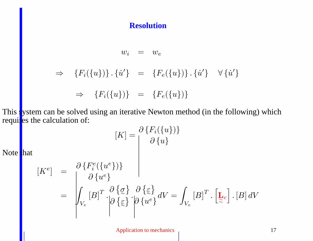
Resolution

wi = we

⇒ Fi(u) . u′ = Fe(u) . u′ ∀ u′

⇒ Fi(u) = Fe(u)

This system can be solved using an iterative Newton method (in the following) whichrequires the calculation of:

[K] =∂ Fi(u)

∂ uNote that

[Ke] =∂ F e

i (ue)∂ ue

=

∫

Ve

[B]T .∂

σ∼

∂

ε∼

.∂

ε∼

∂ uedV =

∫

Ve

[B]T .[

L∼∼

c

]

. [B] dV


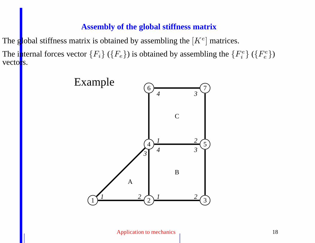
Assembly of the global stiffness matrix

The global stiffness matrix is obtained by assembling the [Ke] matrices.

The internal forces vector Fi (Fe) is obtained by assembling the F ei (F e

e )vectors.

Example

1 2 3

4 5

6 7

A

B

C

1 2

3

1 2

34

1 2

34


u =

u1x, u1

y, u2x, u2

y, u3x, u3

y, u4x, u4

y, u5x, u5

y, u6x, u6

y, u7x, u7

y

For element A, the local unknown vector

uA

is:

uA

=

uA1x , uA1

y , uA2x , uA2

y , uA3x , uA3

y

=

u1x, u1

y, u2x, u2

y, u4x, u4

y

The associated internal forces vector associated to element A is:

FAi

=

FA1x , FA1

y , FA2x , FA2

y , FA3x , FA3

y


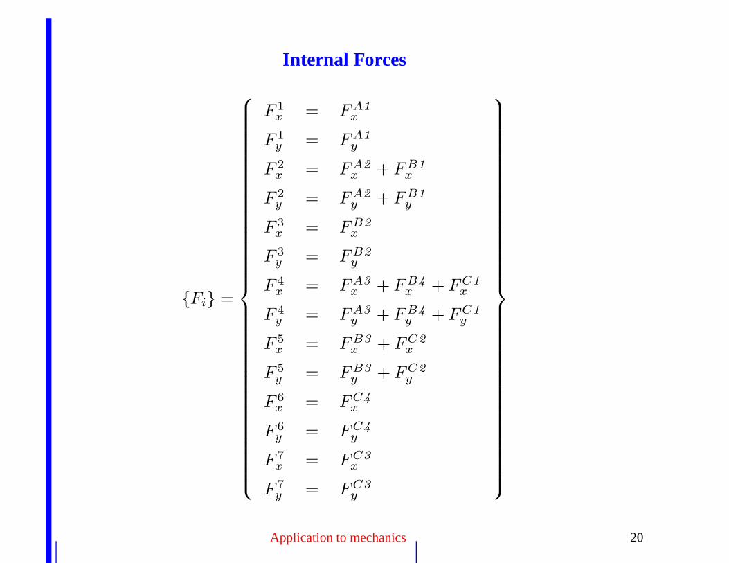
Internal Forces

Fi =

F 1x = FA1

x

F 1y = FA1

y

F 2x = FA2

x + FB1x

F 2y = FA2

y + FB1y

F 3x = FB2

x

F 3y = FB2

y

F 4x = FA3

x + FB4x + FC1

x

F 4y = FA3

y + FB4y + FC1

y

F 5x = FB3

x + FC2x

F 5y = FB3

y + FC2y

F 6x = FC4

x

F 6y = FC4

y

F 7x = FC3

x

F 7y = FC3

y


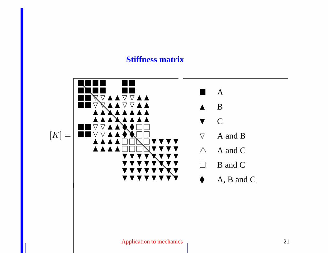
Stiffness matrix

[K] =

OO OONNNNOO OONNNN

NNNNNNNNNNNNNNNN

OONN OONN

NNNNNNNN

HHHHHHHH

HHHHHHHHHHHHHHHHHHHHHHHHHHHHHHHH

A

N B

H C

O A and B

4 A and C

B and C

A, B and C


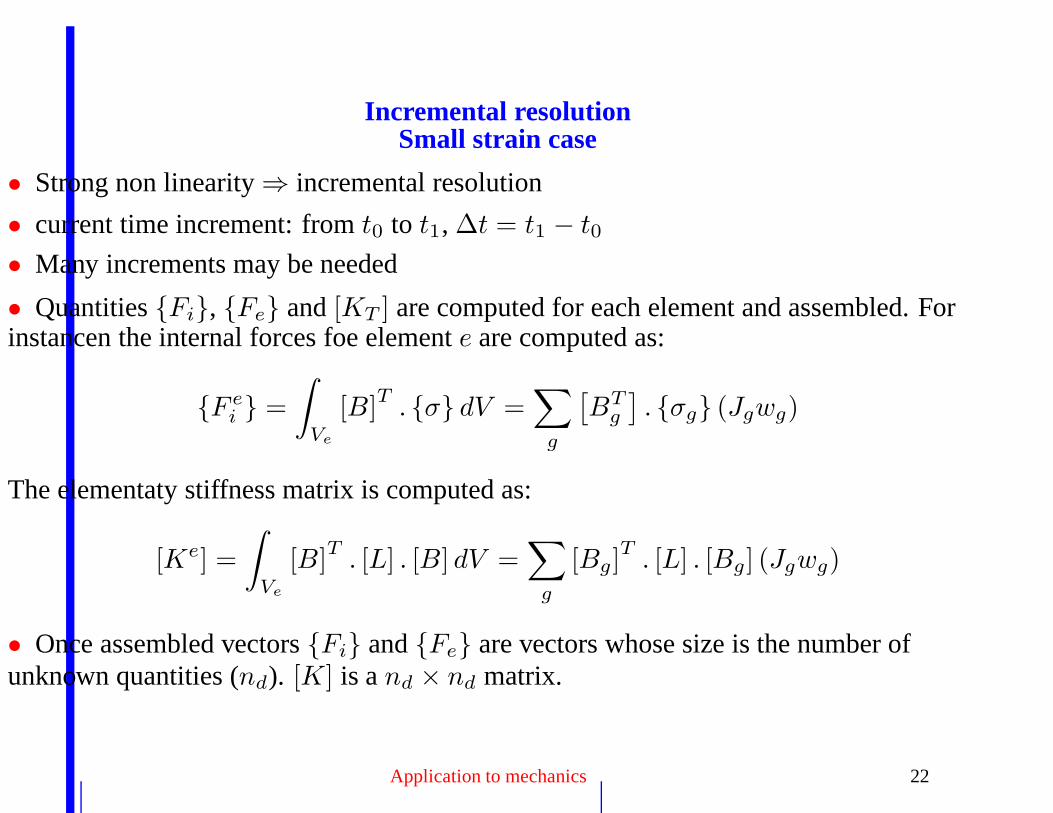
Incremental resolutionSmall strain case

• Strong non linearity ⇒ incremental resolution

• current time increment: from t0 to t1, ∆t = t1 − t0

• Many increments may be needed

• Quantities Fi, Fe and [KT ] are computed for each element and assembled. Forinstancen the internal forces foe element e are computed as:

F ei =

∫

Ve

[B]T . σ dV =∑

g

[

BTg

]

. σg (Jgwg)

The elementaty stiffness matrix is computed as:

[Ke] =

∫

Ve

[B]T . [L] . [B] dV =∑

g

[Bg]T . [L] . [Bg] (Jgwg)

• Once assembled vectors Fi and Fe are vectors whose size is the number ofunknown quantities (nd). [K] is a nd × nd matrix.


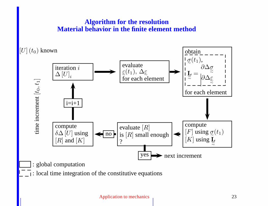
Algorithm for the resolutionMaterial behavior in the finite element method

[U ] (t0) known

time

incr

emen

t[t 0

,t1]

iteration i∆ [U ]i

evaluateε∼(t1), ∆ε

∼

for each element

obtainσ∼(t1),

L∼∼

=∂∆σ

∼∼

∂∆ε∼∼

for each element

compute[F ] using σ

∼(t1)

[K] using L∼∼

evaluate [R]is [R] small enough?

computeδ∆ [U ] using[R] and [K]

i=i+1

no

yes next incrementbox : global computation

box : local time integration of the constitutive equations


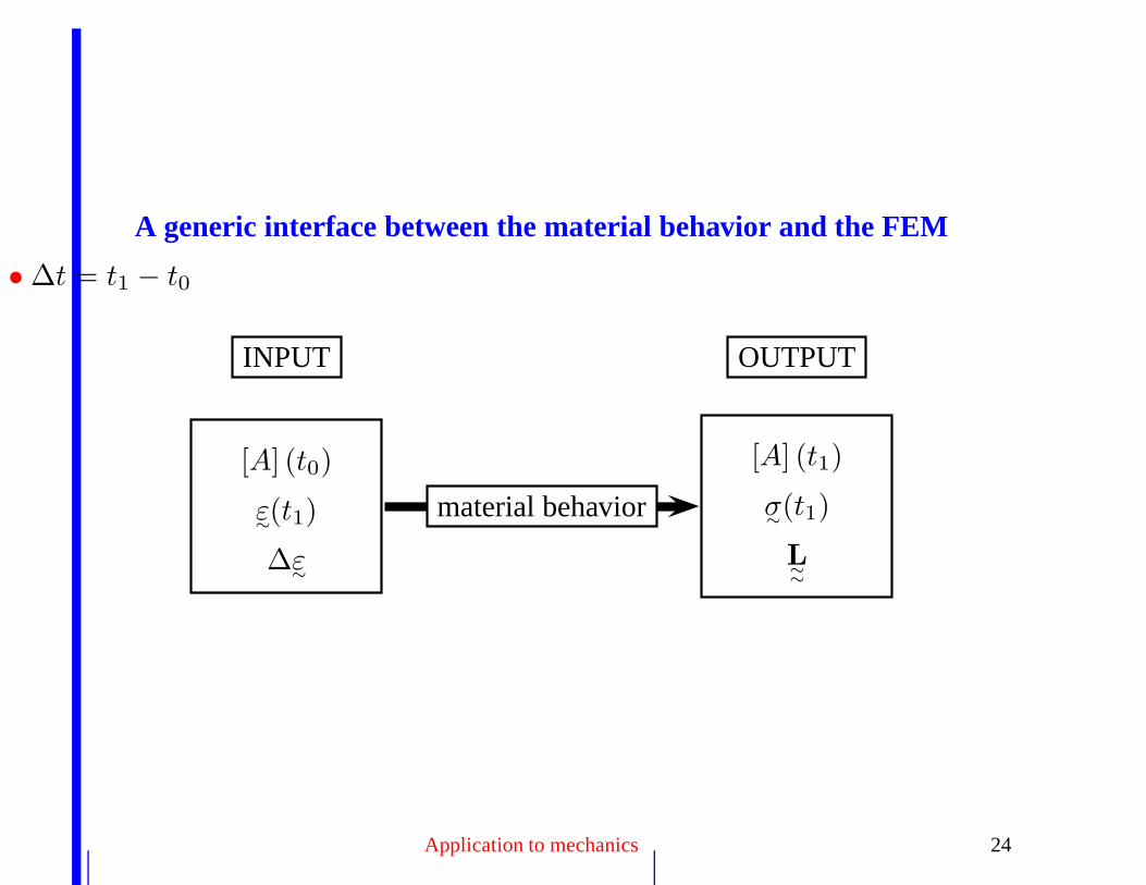
A generic interface between the material behavior and the FEM

• ∆t = t1 − t0

INPUT OUTPUT

[A] (t0)

ε∼(t1)

∆ε∼

[A] (t1)

σ∼(t1)

L∼∼

material behavior


Numerical methods to solve not linear systems of equationsNon linear equations written as:

R (U) = 0FEM case:

Fi (u) − Fe (u) = 0

Solving not linear systems of equations 25

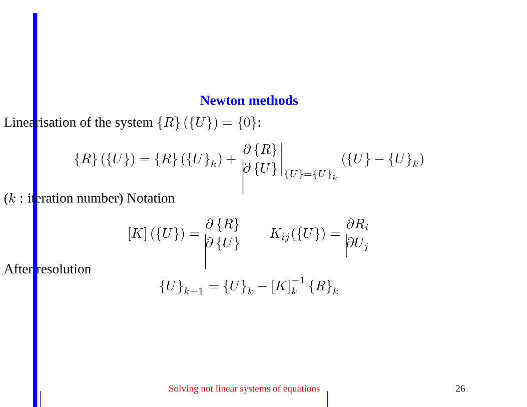
Newton methods

Linearisation of the system R (U) = 0:

R (U) = R (Uk) +∂ R∂ U

∣

∣

∣

∣

U=Uk

(U − Uk)

(k : iteration number) Notation

[K] (U) =∂ R∂ U Kij(U) =

∂Ri

∂Uj

After resolutionUk+1

= Uk − [K]−1

k Rk


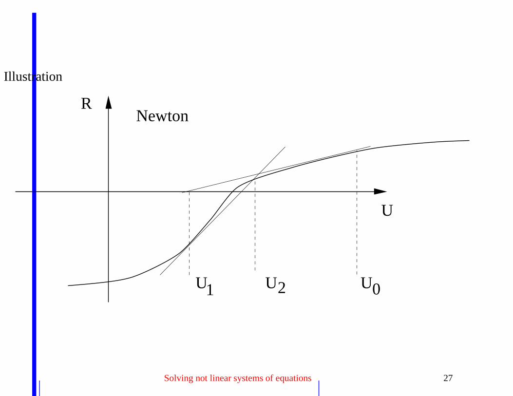
Illustration

R

UU U1 2 0

Newton

U


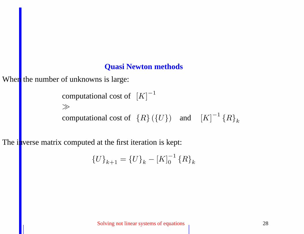
Quasi Newton methods

When the number of unknowns is large:

computational cost of [K]−1

computational cost of R (U) and [K]

−1 Rk

The inverse matrix computed at the first iteration is kept:

Uk+1= Uk − [K]−1

0Rk


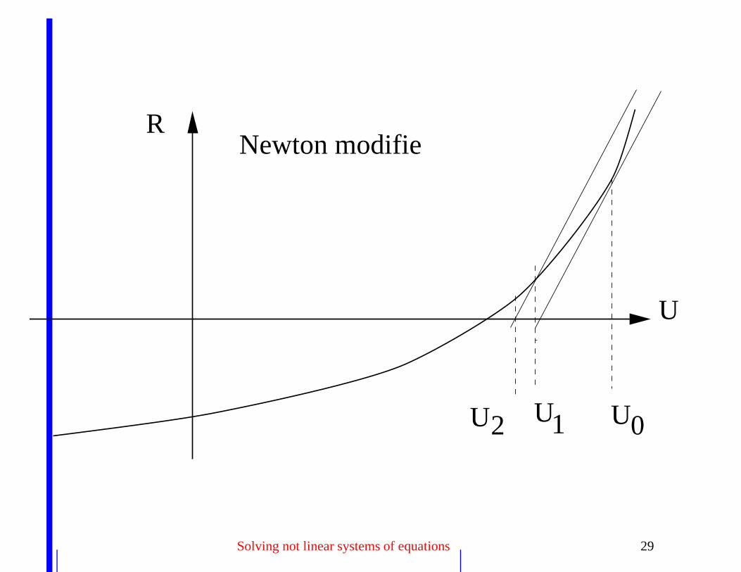
U0U1U2

RNewton modifie

U


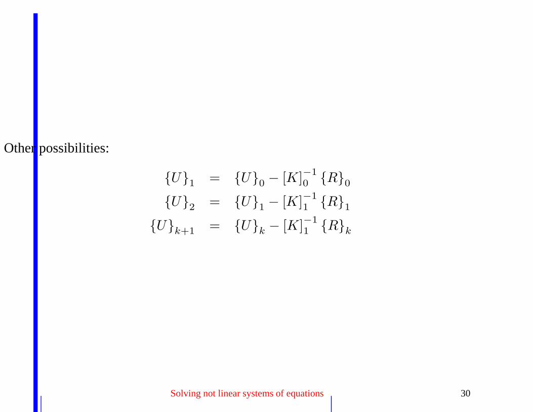
Other possibilities:

U1

= U0− [K]

−1

0R

0

U2

= U1− [K]−1

1R

1

Uk+1= Uk − [K]

−1

1Rk


One unknown case : order of convergence

Fixed Point Method

to be solved (x is scalar):f (x) = 0

Transformation:x = g (x)

Solution : fixed point .

Iterative resolution. x0 is given.xn+1 = g (xn)

Let s be the solution of x = g (x).

If there exits an interval around s such that |g′| ≤ K < 1

then the xn serie converges toward s.


To prove this, one first notices that there exists value t (t ∈ [x, s]) such that (Mean ValueTheorem)

g (x) − g (s) = g′ (t) (x − s)

as g (s) = s et xn = g (xn−1), one gets :

|xn − s| = |g (xn−1) − g (s) | ≤ |g′ (t) ||xn−1 − s|≤ K|xn−1 − s|≤ · · · ≤ Kn|x0 − s|

as K < 1, lim→∞ |xn − s| = 0.


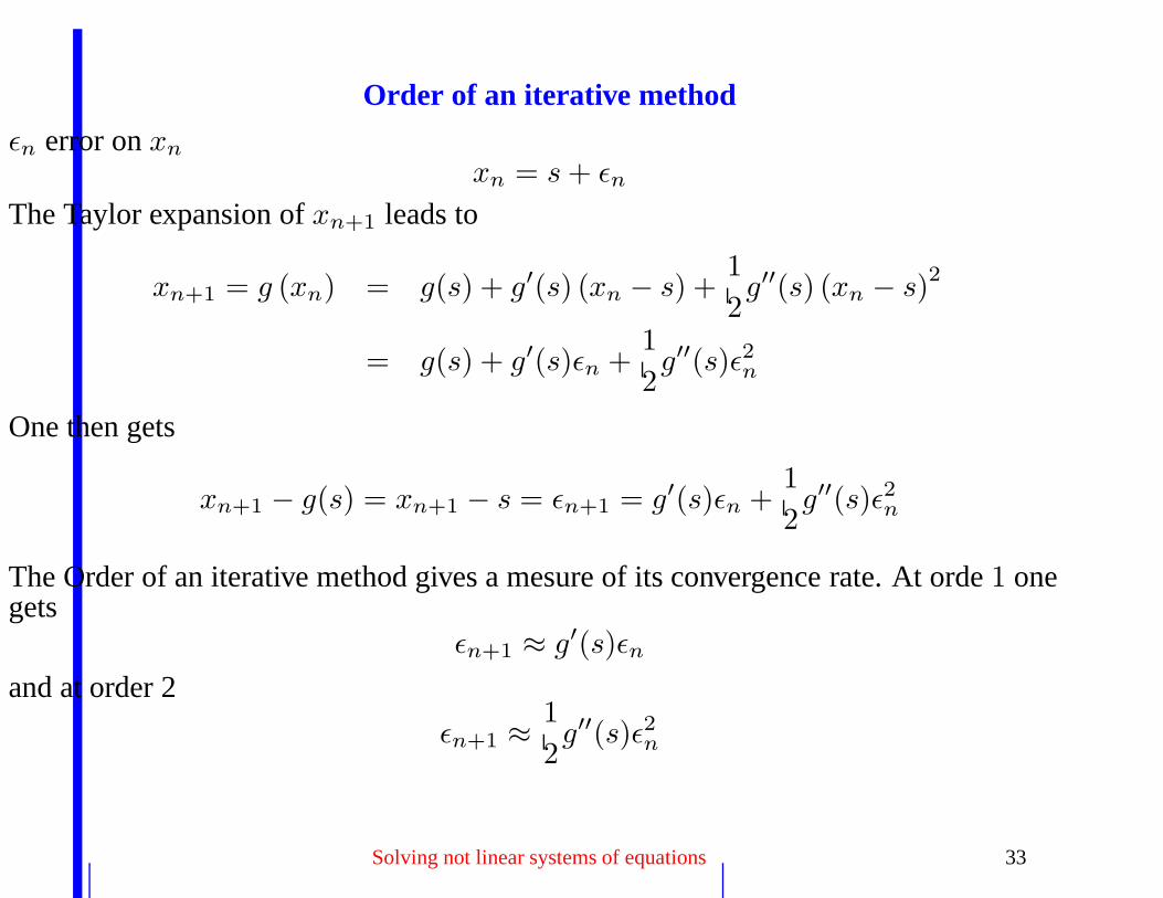
Order of an iterative method

εn error on xn

xn = s + εn

The Taylor expansion of xn+1 leads to

xn+1 = g (xn) = g(s) + g′(s) (xn − s) +1

2g′′(s) (xn − s)2

= g(s) + g′(s)εn +1

2g′′(s)ε2n

One then gets

xn+1 − g(s) = xn+1 − s = εn+1 = g′(s)εn +1

2g′′(s)ε2n

The Order of an iterative method gives a mesure of its convergence rate. At orde 1 onegets

εn+1 ≈ g′(s)εn

and at order 2

εn+1 ≈ 1

2g′′(s)ε2n


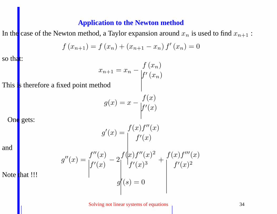
Application to the Newton method

In the case of the Newton method, a Taylor expansion around xn is used to find xn+1 :

f (xn+1) = f (xn) + (xn+1 − xn) f ′ (xn) = 0

so that:

xn+1 = xn − f (xn)

f ′ (xn)

This is therefore a fixed point method

g(x) = x − f(x)

f ′(x)

One gets:

g′(x) =f(x)f ′′(x)

f ′(x)

and

g′′(x) =f ′′(x)

f ′(x)− 2

f(x)f ′′(x)2

f ′(x)3+

f(x)f ′′′(x)

f ′(x)2

Note that !!!g′(s) = 0


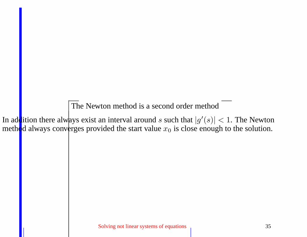
The Newton method is a second order method

In addition there always exist an interval around s such that |g′(s)| < 1. The Newtonmethod always converges provided the start value x0 is close enough to the solution.


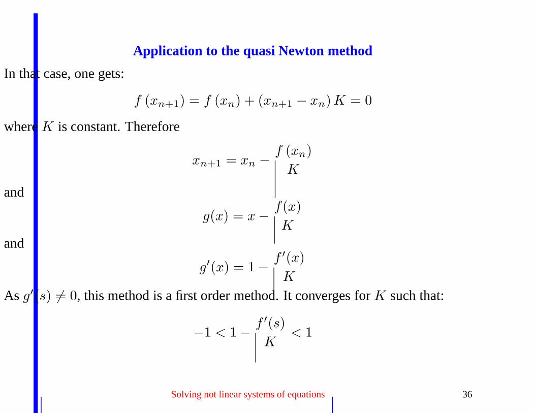
Application to the quasi Newton method

In that case, one gets:

f (xn+1) = f (xn) + (xn+1 − xn) K = 0

where K is constant. Therefore

xn+1 = xn − f (xn)

K

and

g(x) = x − f(x)

K

and

g′(x) = 1 − f ′(x)

K

As g′(s) 6= 0, this method is a first order method. It converges for K such that:

−1 < 1 − f ′(s)

K< 1


Riks methodControl

The “natural” problem control mode is to impose the external forces Fe. This controlworks if the load increases with displacement.

In the case of a limit load, a displacement control is needed.

In the case of snap-back instabilities, a mixte load—a displacement control is needed.


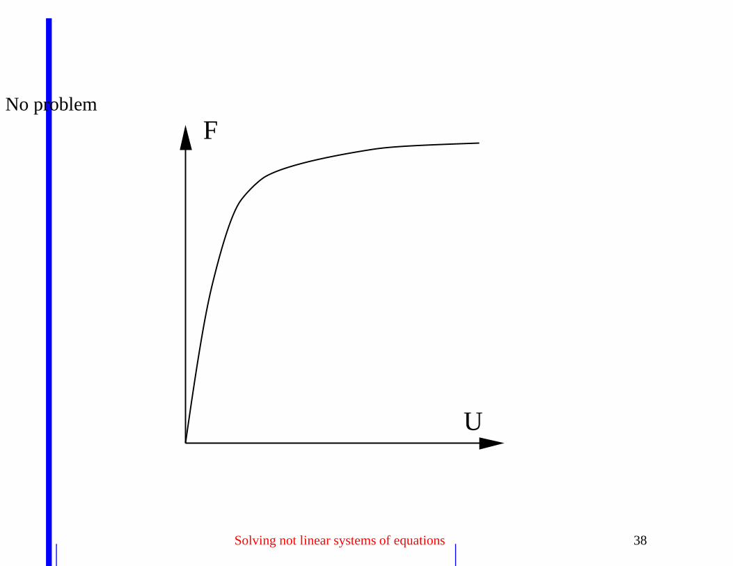
No problem

U

F


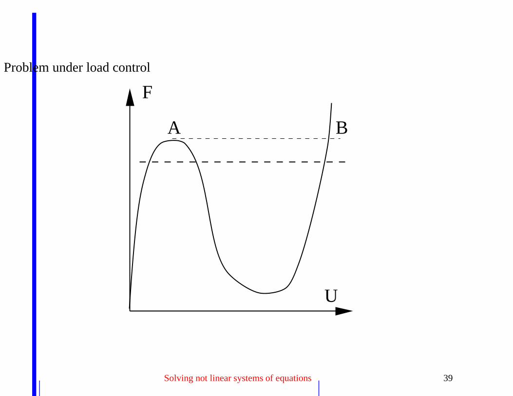
Problem under load control

U

F

A B


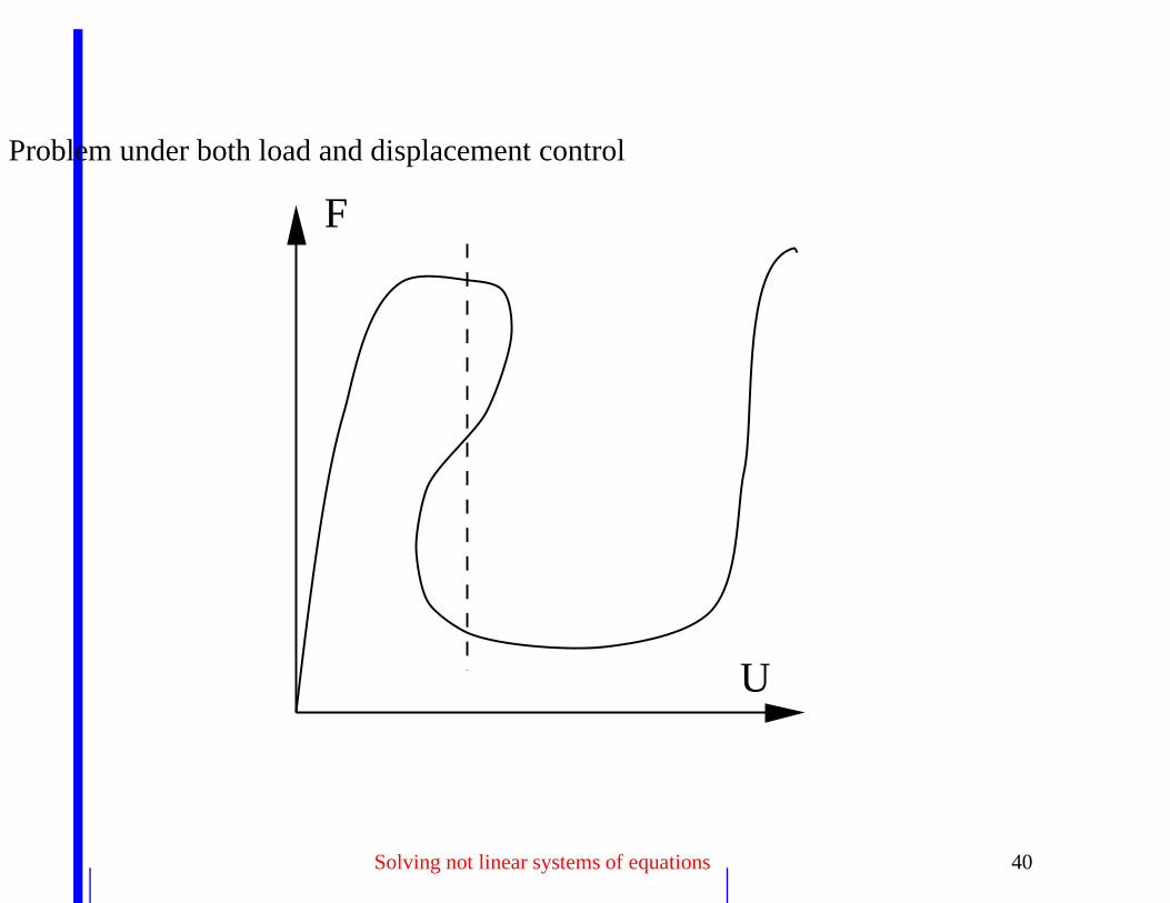
Problem under both load and displacement control

U

F


Convergence

The convergence of the iterative resolution can be tested according to different methods:

• As the search solution verifies: R = 0, the iterative process is stopped whenR is small enough:

||R||n < Rε

where Rε is the requested precision. With

||R||n =

(

∑

i

Rni

)1

n

The ”inf.” norm is often used:

||R||∞ = maxi

|Ri|

• In many cases, the equation R = 0 can be written as: Ri − Re = 0where Re is prescribed. A relative error can then be defined:

||Ri − Re||||Re||

< rε

where rε is the requested precision. Note that in some cases (residual stresses during


cooling) Re = 0 so that a relative error cannot be defined.

• The search can be stopped when the approximate solution is stable, i.e.∣

∣

∣

∣Uk+1− Uk

∣

∣

∣

∣

n< Uε

This is not a strict convergence criterion For instance the serie: xn = log n verifiesthe criterion (xn+1 − xn = log((n + 1)/n)) ibut does not converge !


Incompressibility / Quasi incompressibilitySome materials are incompressible or quasi–incompressible (rubber, metals duringforming, etc. . . ).

The incompressibility condition is written as: La condition d’incompressibilité se traduitpar la condition

div (u) = 0

A FE formulation based on displacement only does not “naturally” enforce thiscondition. An enriched method must be used.

The stress tensor can be separated into a deviatoric component s∼

and an hydrostaticcomponent p so that: que l’on a :

σ∼

= s∼− p1

∼

Incompressibility 43

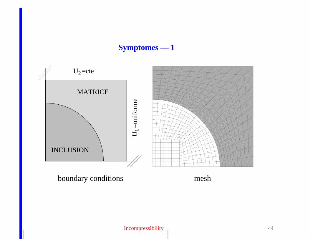
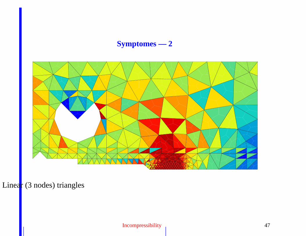
Symptomes — 1

U =

unif

orm

e1

U =cte2

MATRICE

INCLUSION

boundary conditions mesh


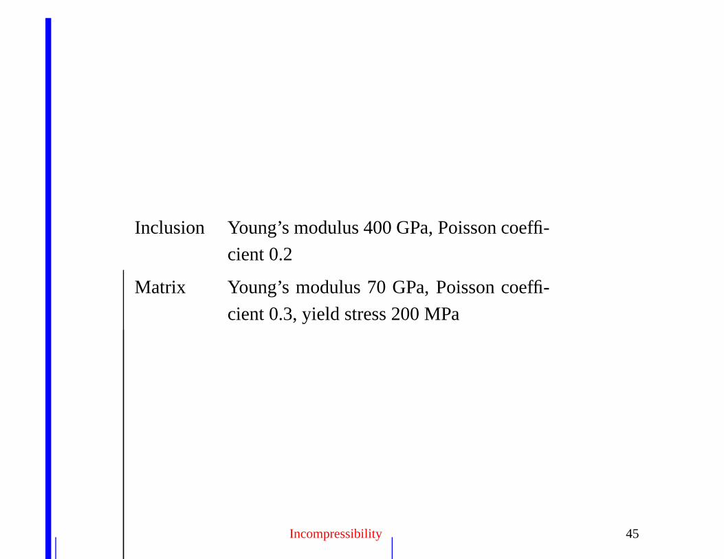
Inclusion Young’s modulus 400 GPa, Poisson coeffi-

cient 0.2

Matrix Young’s modulus 70 GPa, Poisson coeffi-

cient 0.3, yield stress 200 MPa


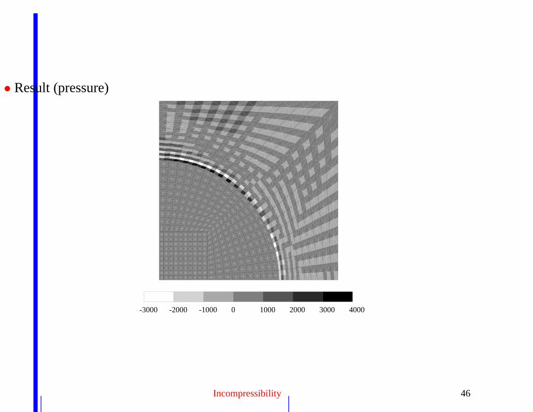
• Result (pressure)

-3000 -2000 -1000 0 1000 2000 3000 4000


Symptomes — 2

Linear (3 nodes) triangles


Solution 1

• The first solution consists in post-processing the data in order to average the pressurewithin each element:

p =1

V

∫

V

pdV

• A new stress field is build:

σ∼

= s∼− p1

∼→ σ

∼

∗ = s∼− p1

∼

• This solution can be useful but is not general (does not work for T3)


Approximated formulation : selective integration

One uses a selective integration of the volume variation.

• The strain tensor is related to the nodal displacement by

ε∼

= [B] . U

• [B] can be separated into a deviatoric part [Bdev] and a dilatation part [Bdil]:

[B] = [Bdev] + [Bdil]

• [Bdil] is then avaraged over the element:

[

Bdil

]

=1

|Ve|

∫

Ve

[Bdil] dV

• A modified [B] is reconstructed;

[B∗] = [Bdev] +[

Bdil

]

• Deformation is then computed using [B∗]:

ε∼

= [B∗] . U


• The volume variation is therefore constant in the element

• Once again the method cannot be applied to linear triangles and tetrahedrons. It can beapplied to quadraric triangles and tetrahedrons


Approximated Formulation : penalisation

• In that case the material behavior is incompressible; this implies that only s∼

and not σ∼

can be obtained from the material. • pressure is computed for each element

p = −κui,i

• κ : numerical penalisation factor (compressibility)• σ

∼= s

∼− p1

∼

• Ifκ is large enough : divu ≈ 0

• Unknowns: displacements U.

• Internes forces are still given by:∫

Ve

[B]T .σ∼dV

• the elementary stiffness matrix is now given by:

[Ke] =

∫

Ve

(

[B]T

.L∼∼

. [B] + λ([B]T

. [m]T) ⊗ ([m] . [B])

)

dV

• [m] = [1 1 1 0 0 0]


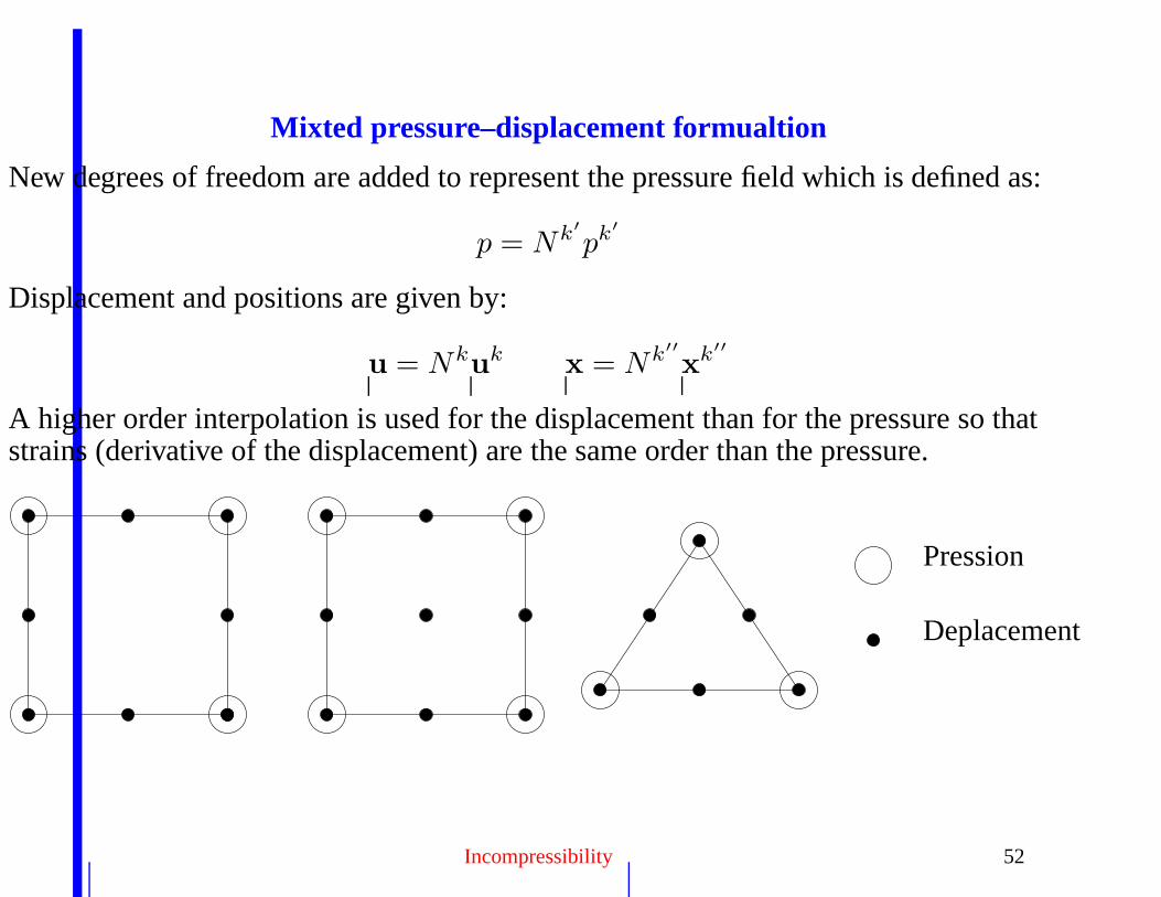
Mixted pressure–displacement formualtion

New degrees of freedom are added to represent the pressure field which is defined as:

p = Nk′

pk′

Displacement and positions are given by:

u = Nku

kx = Nk′′

xk′′

A higher order interpolation is used for the displacement than for the pressure so thatstrains (derivative of the displacement) are the same order than the pressure.

Pression

Deplacement


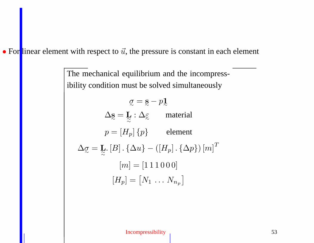
• For linear element with respect to ~u, the pressure is constant in each element

The mechanical equilibrium and the incompress-

ibility condition must be solved simultaneously

σ∼

= s∼− p1

∼

∆s∼

= L∼∼

: ∆ε∼

material

p = [Hp] p element

∆σ∼

= L∼∼

. [B] . ∆u − ([Hp] . ∆p) [m]T

[m] = [1 1 1 0 0 0]

[Hp] =[

N1 . . . Nnp

]


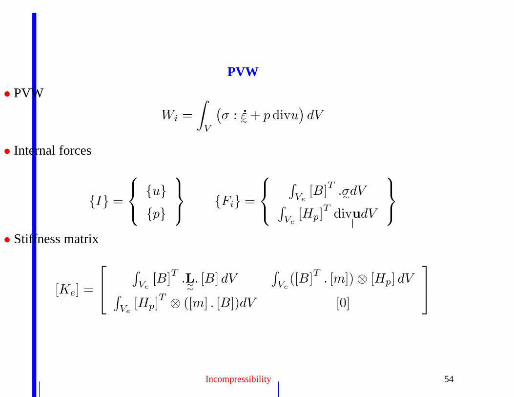
PVW

• PVW

Wi =

∫

V

(

σ : ε∼

+ p divu)

dV

• Internal forces

I =

up

Fi =

∫

Ve[B]T .σ

∼dV

∫

Ve[Hp]

TdivudV

• Stiffness matrix

[Ke] =

∫

Ve[B]

T.L∼∼

. [B] dV∫

Ve([B]

T. [m]) ⊗ [Hp] dV

∫

Ve[Hp]

T ⊗ ([m] . [B])dV [0]


j. besson centre des matériaux, École des mines de paris,...

Documents