j. fluid mech. (2017), . 829, pp. … · at high grashof numbers are examined using direct...
TRANSCRIPT

J. Fluid Mech. (2017), vol. 829, pp. 589–620. c© Cambridge University Press 2017doi:10.1017/jfm.2017.372
589
Direct numerical simulation of turbulent slopeflows up to Grashof number Gr= 2.1× 10¹¹
M. G. Giometto1,†, G. G. Katul2, J. Fang3 and M. B. Parlange1,‡1Department of Civil Engineering, University of British Columbia, Vancouver, BC V6T 1Z4, Canada
2Nicholas School of the Environment, Duke University, Durham, NC 27708, USA3School of Architecture, Civil and Environmental Engineering, École Polytechnique Fédérale de
Lausanne, Lausanne, VD 1015, Switzerland
(Received 26 April 2016; revised 20 May 2017; accepted 25 May 2017;first published online 22 September 2017)
Stably stratified turbulent flows over an unbounded, smooth, planar sloping surfaceat high Grashof numbers are examined using direct numerical simulations (DNS).Four sloping angles (α = 15◦, 30◦, 60◦ and 90◦) and three Grashof numbers(Gr = 5 × 10¹⁰, 1 × 10¹¹ and 2.1 × 10¹¹) are considered. Variations in meanflow, second-order statistics and budgets of mean- (MKE) and turbulent-kineticenergy (TKE) are evaluated as a function of α and Gr at fixed molecular Prandtlnumber (Pr= 1). Dynamic and energy identities are highlighted, which diagnose theconvergence of the averaging operation applied to the DNS results. Turbulent anabatic(upward moving warm fluid along the slope) and katabatic (downward moving coldfluid along the slope) regimes are identical for the vertical wall set-up (up to thesign of the along-slope velocity), but undergo a different transition in the mechanismssustaining turbulence as the sloping angle decreases, resulting in stark differences atlow α. In addition, budget equations show how MKE is fed into the system throughthe imposed surface buoyancy, and turbulent fluctuations redistribute it from thelow-level jet (LLJ) nose towards the boundary and outer flow regions. Analysis ofthe TKE budget equation suggests a subdivision of the boundary layer of anabaticand katabatic flows into four distinct thermodynamical regions: (i) an outer layer,corresponding approximately to the return flow region, where turbulent transport isthe main source of TKE and balances dissipation; (ii) an intermediate layer, boundedbelow by the LLJ and capped above by the outer layer, where the sum of shear andbuoyant production overcomes dissipation, and where turbulent and pressure transportterms are a sink of TKE; (iii) a buffer layer, located at 5 / z+ / 30, where TKEis provided by turbulent and pressure transport terms, to balance viscous diffusionand dissipation; and (iv) a laminar sublayer, corresponding to z+ / 5, where theinfluence of viscosity is significant. (·)+ denotes a quantity rescaled in inner units.Interestingly, a zone of global backscatter (energy transfer from the turbulent eddiesto the mean flow) is consistently found in a thin layer below the LLJ in both anabaticand katabatic regimes.
Key words: atmospheric flows, boundary layer structure, meteorology
† Email address for correspondence: [email protected]‡ Department of Civil and Environmental Engineering, Monash University, Clayton,
VIC 3800, Australia.
Dow
nloa
ded
from
htt
ps://
ww
w.c
ambr
idge
.org
/cor
e. D
uke
Uni
vers
ity L
ibra
ries
, on
03 N
ov 2
017
at 1
4:53
:15,
sub
ject
to th
e Ca
mbr
idge
Cor
e te
rms
of u
se, a
vaila
ble
at h
ttps
://w
ww
.cam
brid
ge.o
rg/c
ore/
term
s. h
ttps
://do
i.org
/10.
1017
/jfm
.201
7.37
2

590 M. G. Giometto, G. G. Katul, J. Fang and M. B. Parlange
1. Introduction
When an inclined surface is thermally altered from the state of the overlyingfluid, the resulting buoyancy force projects in both the along- and normal-to-slopedirections. Surface cooling results in a downslope flow (katabatic flow), whereassurface heating generates an upslope flow (anabatic flow). The significance of suchsloping turbulent flows is rarely questioned given their ubiquity and their central rolein land–atmosphere exchange processes. Katabatic and anabatic flows are persistentover complex terrains (Whiteman 1990; Monti et al. 2002; Rampanelli, Zardi &Rotunno 2004; Haiden & Whiteman 2005; Rotach & Zardi 2007; Fernando 2010;Zardi & Whiteman 2013; Nadeau et al. 2013a; Oldroyd et al. 2014, 2016b; Fernandoet al. 2015; Lehner et al. 2015; Grachev et al. 2016; Hang et al. 2016; Jensenet al. 2016), and despite their local nature, their interaction with larger-scale forcingmechanisms can favour the development of cyclonic vorticity in the middle and uppertroposphere (Parish 1992; Parish & Bromwich 1998). Katabatic winds regulate energy,momentum and mass transfer over the ice sheets of Greenland and Antarctica (Egger1985; Parish 1992; Parish & Bromwich 1998; Renfrew 2004; Renfrew & Anderson2006), and also influence the movement of the marginal ice zone (Chu 1987). Inaddition, katabatic flows are a permanent feature of the atmospheric boundary layer(ABL) over melting glaciers (Greuell et al. 1994; Smeets, Duynkerke & Vugts1997; Oerlemans 1998; Oerlemans et al. 1999; Smeets, Duynkerke & Vugts 2000;Parmhed, Oerlemans & Grisogono 2004), whose constant retreat is a matter ofpublic interest, given their impact on both the sea level rise and on water resourcemanagement.
Prandtl (1942) framed the problem of slope flows in a conceptually simple model,considering a doubly infinite (no leading edges) plate that is uniformly heated orcooled and lies within a stably stratified environment. The Prandtl model (Prandtl1942) states that the advection of base-state (environmental) potential temperatureis balanced by buoyancy (diffusive) flux divergence, whereas the slope-parallelcomponent of buoyancy balances momentum (diffusive) flux divergence. Thisparticular type of flows are termed equilibrium flows (Mahrt 1982), given the natureof the balance between a turbulent flux divergence and a generation/destructionmechanism. Under such settings, the Boussinesq equations of motion and thermalenergy reduce to one-dimensional form, which allows for analytical treatment.Accounting for a base stable stratification admits solutions that approach steady-stateconditions at large times, whereas in the absence of a stable stratification (classicalsolutions), the thermal and dynamic boundary layers (TBL and DBL in the following)grow in an unbounded manner (Menold & Yang 1962).
The original model assumed constant turbulent diffusivities (labelled as K) – andis therefore incapable of representing the observed steep near-surface gradients(Grisogono & Oerlemans 2001b). In addition, the return flow region predictedby the constant-K solution is usually stronger, when compared to measurementsor numerical simulations, and also vanishes more rapidly away from the surface(Defant 1949; Denby 1999; Grisogono & Oerlemans 2001b). This limitation wasfirst overcome in Gutman (1983), where a patched analytic solution was proposed,valid for linearly decreasing K in the inner flow regions. More recently, Grisogono &Oerlemans (2001b, 2002) proposed an approximate analytical solution able to accountfor gradually varying eddy diffusivities, valid under the WKB approximation (afterWentzel–Kramers–Brillouin), and a closed form solution valid for O’Brien type K wasderived in Giometto et al. (2017). Modifications of the Prandtl model to allow for
Dow
nloa
ded
from
htt
ps://
ww
w.c
ambr
idge
.org
/cor
e. D
uke
Uni
vers
ity L
ibra
ries
, on
03 N
ov 2
017
at 1
4:53
:15,
sub
ject
to th
e Ca
mbr
idge
Cor
e te
rms
of u
se, a
vaila
ble
at h
ttps
://w
ww
.cam
brid
ge.o
rg/c
ore/
term
s. h
ttps
://do
i.org
/10.
1017
/jfm
.201
7.37
2
Direct numerical simulation of turbulent slope flows 591
variations in surface forcing (Shapiro & Fedorovich 2007, 2008; Burkholder, Shapiro& Fedorovich 2009), to account for Coriolis effects (Kavavcic & Grisogono 2007;Shapiro & Fedorovich 2008), time dependence of the solution (Shapiro & Fedorovich2004, 2005, 2008; Zardi & Serafin 2015) and for weakly nonlinear effects (Grisogonoet al. 2014; Güttler et al. 2016), were also recently proposed.
The Prandtl conceptual approach is also of interest in numerical modelling. Italleviates computational costs by constraining the geometry to regular domains,thus allowing the use of efficient numerical schemes such as methods based onfinite differences or spectral expansions. The existence of a statistically steady-statesolution also provides a benchmark for quantitative analysis. The past decadeshave seen significant advances in computational performance, achieved through bothimprovements in computer hardware and in numerical algorithms that solve differentialequations. Nevertheless, computational cost of simulating high Reynolds number (Re)flows over long slopes remains prohibitively high, and has motivated the use ofclosure models that aim at reducing resolution requirements in the dissipative range,especially when energy-containing scales are of primary interest (Pope 2000). Sincethe pioneering work of Schumann (1990), large-eddy simulation (LES) has representedone of the workhorses for the simulation of slope flows within the Prandtl modelframework. It has revealed several aspects of the turbulent structure and illustratedthe sensitivity of the bulk solution to the system parameters (Skyllingstad 2003;Axelsen & Dop 2009a,b; Grisogono & Axelsen 2012). LES of slope flows in morecomplex configurations (i.e. not relying on the Prandtl model set-up) have beenperformed in Smith & Skyllingstad (2005), where the effects of varying slope anglewere analysed, and the interaction of slope flows with valley systems have also beenrecently addressed via LES (Chow et al. 2006; Weigel et al. 2006; Chemel, Staquet& Largeron 2009; Burns & Chemel 2014, 2015; Arduini, Staquet & Chemel 2016).However, the stable stratification and the peculiar features characterizing slope flows(e.g. the presence of zero-gradient layers in the state variables) question the validity ofthe assumptions upon which LES subgrid-scale (SGS) models are derived (Burkholder,Fedorovich & Shapiro 2011). In addition, the lack of a rigorous similarity theory forslope flows (Mahrt 1998; Grisogono & Oerlemans 2001a; Grisogono, Kraljevic &Jericevic 2007; Mahrt 2013; Nadeau et al. 2013b; Monti, Fernando & Princevac 2014;Oldroyd et al. 2016a) makes it impossible to prescribe adequate surface fluxes insimulations. These limitations have motivated the use of direct numerical simulations(DNS), which, despite their modest range of Re, provide the most comprehensive viewof the flow structure (Fedorovich & Shapiro 2009) (FS09 hereafter). These studiesshowed that slope-flow statistics are sensitive to variations in the parameter space,including the magnitude of the surface forcing, the slope angle and the strength ofthe ambient stratification. They all play a role in determining the characteristics of theflow. This finding motivated recent efforts towards a derivation of scaling relationsthat allow the elimination of the dependency of the solution on the sloping angle(Shapiro & Fedorovich 2014). Scaling relations are of interest since they facilitate thedesign of experiments and have potentials to yield significant computational savingsin parametric studies when explored through LES and DNS.
In this work, the problem of anabatic and katabatic flows and the propertiesof the LLJ in the near-wall region are explored using high resolution DNS. Thefocus is on variations in the slope-normal structure of selected flow statistics andin integrated quantities as a function of the sloping angle (α) and of the Grashofnumber (Gr). The flow is driven by a homogeneous constant surface buoyancy forceand the molecular Prandtl number (Pr) is set to unity (instead of a typical 0.7 value
Dow
nloa
ded
from
htt
ps://
ww
w.c
ambr
idge
.org
/cor
e. D
uke
Uni
vers
ity L
ibra
ries
, on
03 N
ov 2
017
at 1
4:53
:15,
sub
ject
to th
e Ca
mbr
idge
Cor
e te
rms
of u
se, a
vaila
ble
at h
ttps
://w
ww
.cam
brid
ge.o
rg/c
ore/
term
s. h
ttps
://do
i.org
/10.
1017
/jfm
.201
7.37
2

592 M. G. Giometto, G. G. Katul, J. Fang and M. B. Parlange
FIGURE 1. Slope-aligned coordinate system.
for air) in line with the FS09 study. The current study complements and extendsthe work of FS09, where a similar set-up was adopted to characterize slope flowsdriven by an imposed surface buoyancy flux. The aim is to shed additional light onthe interactions between turbulence and the mean flow state as well as the role ofthe low-level jet (LLJ) in energy and momentum exchanges. Specifically, the studyaims at (i) assessing how α and Gr influence katabatic and anabatic flows whenconstant surface buoyancy is prescribed; (ii) contrasting key features between slopeflows driven by a constant imposed surface buoyancy, when compared against slopeflows generated by a constant imposed surface buoyancy flux; and (iii) characterizingthe vertical structures (and their sensitivity to variations in the parameter space) ofmean kinetic energy (MKE) and of turbulent kinetic energy (TKE) budget terms. Thelong-term goal is to provide improvements for current turbulence closure models forsloping and stable conditions that can then be implemented in large-scale atmosphericmodels so as to address the plethora of problems already highlighted earlier on inthe introduction. The manuscript is organized as follows. The governing equations forthe problem are derived in § 2. Section 3 provides details on the numerical algorithmand on the set-up of simulations and the main results are presented in § 4. Summaryand concluding remarks follow in § 5.
2. Equations of motion
Thermal convection of turbulent stratified fluid flow over sloping surfaces canbe described in a slope-rotated reference system, where x is the along-slopedirection, y denotes the spanwise direction and z is the slope-normal direction, asdisplayed in figure 1. (·) indicates a dimensional variable. The potential temperatureθ (x, t) is decomposed into a base state θR(z∗) and a perturbation componentθ ′′(x, t) ≡ θ (x, t) − θR(z∗) as originally proposed by Prandtl (1942). Assuming thebase state θR(z∗) to be a linear function of the vertical coordinate direction z∗, results
in N ≡√β(dθR/dz∗)= const., where N is the buoyancy frequency (equivalent to the
Brunt–Väisälä frequency). The thermal expansion coefficient β ≡ g/θ0 where g isthe acceleration due to gravity and θ0 is a reference constant temperature. Moreover,invoking the Boussinesq approximation (i.e. ignoring density differences except wherethey appear in terms multiplied by g) and neglecting earth rotation effects, the
Dow
nloa
ded
from
htt
ps://
ww
w.c
ambr
idge
.org
/cor
e. D
uke
Uni
vers
ity L
ibra
ries
, on
03 N
ov 2
017
at 1
4:53
:15,
sub
ject
to th
e Ca
mbr
idge
Cor
e te
rms
of u
se, a
vaila
ble
at h
ttps
://w
ww
.cam
brid
ge.o
rg/c
ore/
term
s. h
ttps
://do
i.org
/10.
1017
/jfm
.201
7.37
2
Direct numerical simulation of turbulent slope flows 593
conservation equations within the DBL and TBL in dimensional form reduce to
∂ ui
∂ t+∂ uiuj
∂ xj=−
∂π
∂ xi+ ν
∂2ui
∂ x2j− βθ ′′(x, t)[δi1 sin α − δi3 cos α], (2.1)
∂ ui
∂ xi= 0, (2.2)
∂θ ′′
∂ t+∂ ujθ
′′
∂ xj=−
∂ ujθR
∂ xj+ κ
∂2θ ′′
∂ x2j, (2.3)
where t (s) denotes time, ui (m s−1), i = 1, 2, 3, are the velocity components inthe three coordinate directions (x, y, z) (m), π ≡ [p − pR(x, z)]/ρ0 (m2 s−2) is thenormalized deviation of kinematic pressure from the background hydrostatic state,ρ0 (kg m−3) is a reference constant density, α (rad) is the slope angle, ν (m2 s−1) andκ (m2 s−1) are the kinematic molecular viscosity and thermal diffusivity coefficients,and δij is the Kronecker Delta function. Molecular dissipation of kinetic energyrepresents an additional source of heat, and should in principle be included inthe equation for θ . However, due to the low velocities involved in slope flowsthis term is small and has thus been neglected. Introducing the buoyancy variableb(x, t)≡ βθ ′′(x, t), and since z∗(x)≡−x sin α + z cos α, equations (2.1)–(2.3) can bere-written as in FS09
∂ ui
∂ t+∂ uiuj
∂ xj=−
∂π
∂ xi+ ν
∂2ui
∂ x2j− b(x, t)[δi1 sin α − δi3 cos α], (2.4)
∂ ui
∂ xi= 0, (2.5)
∂ b∂ t+∂ ujb∂ xj= N2[u1 sin α − u3 cos α] + κ
∂2b∂ x2
j. (2.6)
2.1. Normalization of the equations and governing parametersTo express the governing equations as a function of suitable dimensionless parameters,a characteristic time, length, buoyancy and velocity scale can be defined as
T ≡ N−1, L≡|bs|
N2, B≡ |bs|, U ≡
|bs|
N, (2.7a−d)
where the surface buoyancy bs determines whether the flow is anabatic (bs > 0) orkatabatic (bs< 0). These aforementioned parameters can now be used to introduce thefollowing normalized variables
t≡ t/T, xi ≡ xi/L, b≡ b/B, ui ≡ ui/U, π≡ π/U2. (2.8a−e)
Relations (2.7) are derived selecting bs and N as repeating parameters though thischoice is by no means unique and other options are possible. Substituting theexpressions (2.8) into the governing equations (2.4)–(2.6) results in
∂ui
∂t+∂uiuj
∂xj=−
∂π
∂xi− b(δi1 sin α − δi3 cos α)+Gr−1/2 ∂
2ui
∂x2j, (2.9)
Dow
nloa
ded
from
htt
ps://
ww
w.c
ambr
idge
.org
/cor
e. D
uke
Uni
vers
ity L
ibra
ries
, on
03 N
ov 2
017
at 1
4:53
:15,
sub
ject
to th
e Ca
mbr
idge
Cor
e te
rms
of u
se, a
vaila
ble
at h
ttps
://w
ww
.cam
brid
ge.o
rg/c
ore/
term
s. h
ttps
://do
i.org
/10.
1017
/jfm
.201
7.37
2

594 M. G. Giometto, G. G. Katul, J. Fang and M. B. Parlange
Label Lx × Ly ×H Nx ×Ny ×Nz α (deg.) T Gr bs
U90H, S90H 0.2412× 0.324 3842
× 1032 90 6.28 2.1× 10¹¹±1
U60H, S60H 0.2412× 0.324 3842
× 1032 60 7.25 2.1× 10¹¹±1
U30H, S30H 0.2412× 0.324 3842
× 1032 30 12.57 2.1× 10¹¹±1
U15H, S15H 0.2412× 0.324 3842
× 1032 15 24.28 2.1× 10¹¹±1
U60M, S60M 0.2412× 0.324 2562
× 1032 60 7.25 1.0× 10¹¹±1
U60L, S60L 0.2412× 0.324 2562
× 1032 60 7.25 5.0× 10¹⁰±1
TABLE 1. Geometry and parameters for the DNS runs. Li and Ni denote the domainsize and the number of collocation nodes in the three coordinate directions, respectively,T denotes the characteristic oscillation period characterizing the buoyancy and velocityfields (see § 3.4), Gr≡ b4
s ν−2 N−6 where bs is the imposed (normalized) surface buoyancy.
Simulation labels indicate whether a specific run is in buoyantly [U]nstable or [S]tableregime (bs = +1 and bs = −1 respectively), the surface sloping angles α, and whichamong the three considered Grashof numbers ([H]igh, [M]edium and [L]ow) is used; forinstance U30H denotes an anabatic flows regime with α = 30◦ at the highest among theconsidered Grashof numbers.
∂ui
∂xi= 0, (2.10)
∂b∂t+∂ujb∂xj= (u1 sin α − u3 cos α)+ (Gr−1/2Pr−1)
∂2b∂x2
j, (2.11)
where Gr≡ b4s ν−2 N−6 is the Grashof number, defined as the ratio between buoyancy
and viscous forces. There are a number of advantages to adopting Gr over otherpossible dimensionless numbers (e.g. Reynolds number). For the particulars ofsloping flow with zero slip at the boundary, Gr measures the relative strength ofthe body (or non-contact) force to the surface (or contact) force arising from friction(or viscosity). The flow adjustment to this imbalance gives rise to non-hydrostaticpressure distribution and advective acceleration.
3. SimulationsEquations (2.9)–(2.11) are integrated across a range of sloping angles, α and Gr
numbers, considering both anabatic (upslope) and katabatic (downslope) flow regimes,as summarized in table 1. Given the computational cost of DNS, variations in Gr arelimited to the α = 60◦ case.
Note that (b, α)→ (−b, α+π) is a symmetry transformation for the system (2.9)–(2.11), and therefore cases U90H and S90H are equivalent up to a change in the signof ui. Because of this symmetry, a heated wall at α = 15◦ is equivalent to a cooledwall at α = 15◦ + 180◦.
The DNS algorithm is a modification of the code previously used to studyland–atmosphere interaction processes (Albertson & Parlange 1999a,b; Kumar et al.2006; Bou-Zeid et al. 2009; Calaf, Meneveau & Meyers 2010; Calaf, Parlange &Meneveau 2011; Giometto et al. 2016; Sharma et al. 2016; Sharma, Parlange &Calaf 2017), to develop and test linear and nonlinear LES subgrid-scale models(Porté-Agel, Meneveau & Parlange 2000; Higgins, Parlange & Meneveau 2003;Bou-Zeid, Meneveau & Parlange 2005; Lu & Porté-Agel 2010; Abkar, Bae & Moin2016), to design surface-flux parameterizations (Hultmark, Calaf & Parlange 2013)
Dow
nloa
ded
from
htt
ps://
ww
w.c
ambr
idge
.org
/cor
e. D
uke
Uni
vers
ity L
ibra
ries
, on
03 N
ov 2
017
at 1
4:53
:15,
sub
ject
to th
e Ca
mbr
idge
Cor
e te
rms
of u
se, a
vaila
ble
at h
ttps
://w
ww
.cam
brid
ge.o
rg/c
ore/
term
s. h
ttps
://do
i.org
/10.
1017
/jfm
.201
7.37
2
Direct numerical simulation of turbulent slope flows 595
and to model scalar transport processes (Chamecki, Meneveau & Parlange 2009).Equations are solved in rotational form to ensure conservation of mass and kineticenergy (Orszag & Pao 1975). A pseudospectral collocation approach (Orszag 1969,1970) based on truncated Fourier expansions is used in the x, y coordinate directionswhereas a second-order accurate centred finite differences scheme is adopted in theslope-normal direction, requiring a staggered grid approach for the u, v, p, b statevariables (these are stored at (i+ 1/2)∆Z , where i denotes a given layer of collocationnodes in the slope-normal direction). Time integration is performed adopting a fullyexplicit second-order accurate Adams–Bashforth scheme. A fractional step method(Chorin 1968; Temam 1968) is adopted to compute the pressure field by solvingan additional Poisson equation, which is derived enforcing mass continuity for theincompressible fluid (∂ui/∂xi = 0). Further, all nonlinear terms are fully de-aliasedadopting a 3/2 rule so as to avoid artificial pile up of energy at the high wavenumberrange (Kravchenko & Moin 1997; Canuto et al. 2006).
Equations are integrated over a regular domain [0, Lx] × [0, Ly] × [0, H], withboundary conditions ui(x, y, 0)= ui(x, y,H)= b(x, y,H)= 0 and b(x, y, 0)= bs/B=±1.
A sponge layer (Israeli & Orszag 1981) is applied to the top 20 % of thecomputational domain so as to damp spurious internal wave reflections. The thicknessof the sponge layer has been chosen based on a sensitivity analysis performed onthe S15H case, which showed that a minimum of 15 % thickness is required to avoidnon-negligible TKE at the top of the computational domain.
To guide the choice of the grid stencil an estimate of η? = Gr−3/8τ−1/4bz for the
α= 90◦ case was first evaluated from the Prandtl laminar flow analytic solution, whereη? is an equivalent of the Kolmogorov scale (FS2009) in the chosen normalized units,and where τbz denotes the normalized kinematic surface buoyancy flux. Subsequentlythe grid stencils were set to ∆x=∆y= 2∆z= 2η?. The resolvability condition ∆< 2η(Pope 2000) has been checked a posteriori (not shown) for all the considered cases,where η=Gr−3/8ε−1/4 is the Kolmogorov length scale in normalized units. The verticalgrid stencil satisfies such a criterion in all cases, whereas the horizontal grid stencilis often off by a factor of two, hence the need to verify the quality of proposedresults. To do so, a higher resolution DNS katabatic run was performed at a slopingangle α = 90◦, halving the horizontal grid stencil (i.e. doubling the resolution in thehorizontal directions). Note that the Kolmogorov scale is usually larger in stable casesthan in the neutral ones, hence slope flows over vertical walls (α = 90◦) have themost stringent resolution requirements. First- and second-order statistics are found tobe in good agreement with those presented herein, supporting the working conjecturethat the current resolution is sufficient to represent most of the dissipative scales. Theresulting domain size (see table 1) allows the representation of coherent structurespopulating the DBL and TBL at all the considered sloping angles (a domain-sizeconvergence study was performed for the anabatic case at α = 15◦ to support suchassertion, and variations of statistics were found to be negligible).
Simulations are run for a minimum of 6T , where T= 2π sin−1 α is the characteristic(normalized) period of internal waves that arise in the system due to the imposedstable background stratification. Statistics are computed over the last 5T for the casesα = 90◦, α = 60◦, and over the last 3T for the cases α = 30◦, α = 15◦ (previoustime steps are disregarded to allow turbulence to fully develop). All simulationsare performed using Pr = 1, in line with previous studies of slope flows (FS09).Throughout, 〈·〉 denotes averaging in time and along spatial coordinates of statisticalhomogeneity (x, y) and fluctuations with respect to time and space averages (〈·〉) areexpressed as (·)′.
Dow
nloa
ded
from
htt
ps://
ww
w.c
ambr
idge
.org
/cor
e. D
uke
Uni
vers
ity L
ibra
ries
, on
03 N
ov 2
017
at 1
4:53
:15,
sub
ject
to th
e Ca
mbr
idge
Cor
e te
rms
of u
se, a
vaila
ble
at h
ttps
://w
ww
.cam
brid
ge.o
rg/c
ore/
term
s. h
ttps
://do
i.org
/10.
1017
/jfm
.201
7.37
2
596 M. G. Giometto, G. G. Katul, J. Fang and M. B. Parlange
0–0.14
–0.07
0
0.07
0.14
20 40 60 80 100 120 140
S90HS60HS30HS15H
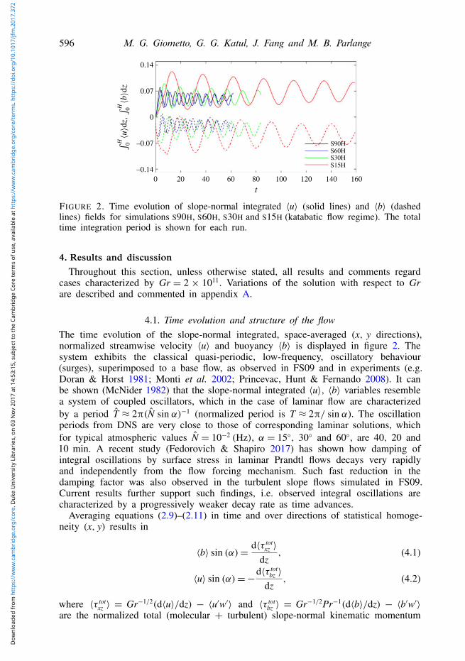
160
FIGURE 2. Time evolution of slope-normal integrated 〈u〉 (solid lines) and 〈b〉 (dashedlines) fields for simulations S90H, S60H, S30H and S15H (katabatic flow regime). The totaltime integration period is shown for each run.
4. Results and discussionThroughout this section, unless otherwise stated, all results and comments regard
cases characterized by Gr = 2 × 10¹¹. Variations of the solution with respect to Grare described and commented in appendix A.
4.1. Time evolution and structure of the flowThe time evolution of the slope-normal integrated, space-averaged (x, y directions),normalized streamwise velocity 〈u〉 and buoyancy 〈b〉 is displayed in figure 2. Thesystem exhibits the classical quasi-periodic, low-frequency, oscillatory behaviour(surges), superimposed to a base flow, as observed in FS09 and in experiments (e.g.Doran & Horst 1981; Monti et al. 2002; Princevac, Hunt & Fernando 2008). It canbe shown (McNider 1982) that the slope-normal integrated 〈u〉, 〈b〉 variables resemblea system of coupled oscillators, which in the case of laminar flow are characterizedby a period T ≈ 2π(N sin α)−1 (normalized period is T ≈ 2π/ sin α). The oscillationperiods from DNS are very close to those of corresponding laminar solutions, whichfor typical atmospheric values N = 10−2 (Hz), α = 15◦, 30◦ and 60◦, are 40, 20 and10 min. A recent study (Fedorovich & Shapiro 2017) has shown how damping ofintegral oscillations by surface stress in laminar Prandtl flows decays very rapidlyand independently from the flow forcing mechanism. Such fast reduction in thedamping factor was also observed in the turbulent slope flows simulated in FS09.Current results further support such findings, i.e. observed integral oscillations arecharacterized by a progressively weaker decay rate as time advances.
Averaging equations (2.9)–(2.11) in time and over directions of statistical homoge-neity (x, y) results in
〈b〉 sin (α)=d〈τ tot
xz 〉
dz, (4.1)
〈u〉 sin (α)=−d〈τ tot
bz 〉
dz, (4.2)
where 〈τ totxz 〉 = Gr−1/2(d〈u〉/dz) − 〈u′w′〉 and 〈τ tot
bz 〉 = Gr−1/2Pr−1(d〈b〉/dz) − 〈b′w′〉are the normalized total (molecular + turbulent) slope-normal kinematic momentum
Dow
nloa
ded
from
htt
ps://
ww
w.c
ambr
idge
.org
/cor
e. D
uke
Uni
vers
ity L
ibra
ries
, on
03 N
ov 2
017
at 1
4:53
:15,
sub
ject
to th
e Ca
mbr
idge
Cor
e te
rms
of u
se, a
vaila
ble
at h
ttps
://w
ww
.cam
brid
ge.o
rg/c
ore/
term
s. h
ttps
://do
i.org
/10.
1017
/jfm
.201
7.37
2
Direct numerical simulation of turbulent slope flows 597
–0.8
–0.4
0
0.4
0.8
1.2
–1.2 –0.8 –0.4 0 0.4 0.8 1.2
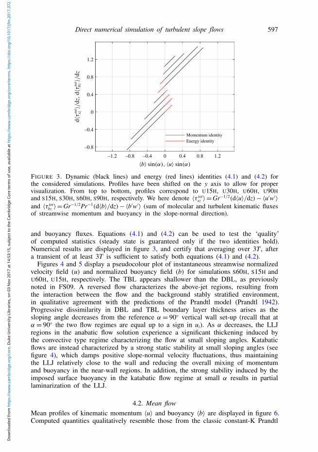
Momentum identityEnergy identity
FIGURE 3. Dynamic (black lines) and energy (red lines) identities (4.1) and (4.2) forthe considered simulations. Profiles have been shifted on the y axis to allow for propervisualization. From top to bottom, profiles correspond to U15H, U30H, U60H, U90Hand S15H, S30H, S60H, S90H, respectively. We here denote 〈τ tot
xz 〉=Gr−1/2(d〈u〉/dz)−〈u′w′〉and 〈τ tot
bz 〉=Gr−1/2Pr−1(d〈b〉/dz)−〈b′w′〉 (sum of molecular and turbulent kinematic fluxesof streamwise momentum and buoyancy in the slope-normal direction).
and buoyancy fluxes. Equations (4.1) and (4.2) can be used to test the ‘quality’of computed statistics (steady state is guaranteed only if the two identities hold).Numerical results are displayed in figure 3, and certify that averaging over 3T , aftera transient of at least 3T is sufficient to satisfy both equations (4.1) and (4.2).
Figures 4 and 5 display a pseudocolour plot of instantaneous streamwise normalizedvelocity field (u) and normalized buoyancy field (b) for simulations S60H, S15H andU60H, U15H, respectively. The TBL appears shallower than the DBL, as previouslynoted in FS09. A reversed flow characterizes the above-jet regions, resulting fromthe interaction between the flow and the background stably stratified environment,in qualitative agreement with the predictions of the Prandtl model (Prandtl 1942).Progressive dissimilarity in DBL and TBL boundary layer thickness arises as thesloping angle decreases from the reference α= 90◦ vertical wall set-up (recall that atα= 90◦ the two flow regimes are equal up to a sign in ui). As α decreases, the LLJregions in the anabatic flow solution experience a significant thickening induced bythe convective type regime characterizing the flow at small sloping angles. Katabaticflows are instead characterized by a strong static stability at small sloping angles (seefigure 4), which damps positive slope-normal velocity fluctuations, thus maintainingthe LLJ relatively close to the wall and reducing the overall mixing of momentumand buoyancy in the near-wall regions. In addition, the strong stability induced by theimposed surface buoyancy in the katabatic flow regime at small α results in partiallaminarization of the LLJ.
4.2. Mean flowMean profiles of kinematic momentum 〈u〉 and buoyancy 〈b〉 are displayed in figure 6.Computed quantities qualitatively resemble those from the classic constant-K Prandtl
Dow
nloa
ded
from
htt
ps://
ww
w.c
ambr
idge
.org
/cor
e. D
uke
Uni
vers
ity L
ibra
ries
, on
03 N
ov 2
017
at 1
4:53
:15,
sub
ject
to th
e Ca
mbr
idge
Cor
e te
rms
of u
se, a
vaila
ble
at h
ttps
://w
ww
.cam
brid
ge.o
rg/c
ore/
term
s. h
ttps
://do
i.org
/10.
1017
/jfm
.201
7.37
2

598 M. G. Giometto, G. G. Katul, J. Fang and M. B. Parlange
0 0.06
0.06
z
z
x x
0.12
0.12
0.18
0.18
0.24 0 0.06
0.06
0.12
0.12
0.18
0.18
0.30
0.24
0.18
0.12
0.06
0
0
–0.25
–0.50
–0.75
–1.00
0.24
0 0.06
0.06
0.12
0.12
0.18
0.18
0.24 0 0.06
0.06
0.12
0.12
0.18
0.18
0.24
(a)
(c)
(b)
(d)
FIGURE 4. Pseudocolour plot of instantaneous katabatic flow streamwise velocity u (a,b)and buoyancy b (c,d), on the plane y = Ly/2 for simulations S60H (a,c) and S15H (b,d).The z-axis denotes the slope-normal coordinate direction, whereas the x-axis denotes thealong-slope direction. The displayed u(x, z) and b(x, z) fields correspond to the crest ofthe last simulated oscillation for both runs. For detailed viewing, only the near-surfaceregion of the total domain is shown.
analytic solution (Prandtl 1942). The most significant features are a peak velocity (uj),the nose of the LLJ (occurring at zj), and a return flow region capping both the DBLand TBL. As previously observed in FS09, such features are sensitive to the slopingangle (α), and as α decreases from the vertical wall set-up (α = 90◦), the anabaticand katabatic flow solutions progressively depart from each other.
The constant-K Prandtl solution provides a useful framework for the interpretationof results, and is thus here briefly summarized. Based on the proposed normalization(see Sect. 2.1), the Prandtl one-dimensional solution for imposed constant surfacebuoyancy reads (FS09)
u=−bsPr−1/2 sin (σ z) exp (−σ z), z ∈ [ 0,∞ ), (4.3)b= bs cos (σ z) exp (−σ z), z ∈ [0,∞), (4.4)
where σ = (Gr Pr−1)1/4 sin (α)1/2 and bs = ±1. Note that (4.3) and (4.4) correspondto a laminar flow solution of the time and space averaged (2.9)–(2.11). It predicts avelocity maximum uj = ±1/
√2 exp (−π/4) that is independent of the sloping angle
(α), whereas the characteristic length scale of the flow L ∝ sin (α)−1/2 whereby zj ∝
sin (α)−1/2 (Grisogono & Axelsen 2012; Grisogono et al. 2014).
Dow
nloa
ded
from
htt
ps://
ww
w.c
ambr
idge
.org
/cor
e. D
uke
Uni
vers
ity L
ibra
ries
, on
03 N
ov 2
017
at 1
4:53
:15,
sub
ject
to th
e Ca
mbr
idge
Cor
e te
rms
of u
se, a
vaila
ble
at h
ttps
://w
ww
.cam
brid
ge.o
rg/c
ore/
term
s. h
ttps
://do
i.org
/10.
1017
/jfm
.201
7.37
2

Direct numerical simulation of turbulent slope flows 599
0 0.06
0.06
z
z
x x
0.12
0.12
0.18
0.18
0.24 0 0.06
0.06
0.12
0.12
0.18
0.18
–0.24
–0.18
–0.12
–0.06
0
0
0.25
0.50
0.75
1.00
0.24
0 0.06
0.06
0.12
0.12
0.18
0.18
0.24 0 0.06
0.06
0.12
0.12
0.18
0.18
0.24
(a)
(c)
(b)
(d)
FIGURE 5. Pseudocolour plot of instantaneous anabatic flow streamwise velocity u (a,b)and buoyancy b (c,d), on the plane y=Ly/2 for simulations U60H (a,c) and U15H (b,d). Thedisplayed u(x, z) and b(x, z) fields correspond to the crest of the last simulated oscillationfor both runs. For detailed viewing, only the near-surface region of the total domain isshown.
The location of the LLJ for the katabatic flow DNS solution is in good agreementwith prediction from the Prandtl laminar flow solution, i.e.
zj ≈π
4σ. (4.5)
Conversely, uj is significantly smaller (a reduction from ≈ 30 % to ≈ 50 % dependingon the slope angle) when compared to the laminar solution, mainly due to additionaldiffusion of momentum caused by turbulent motions at zj (as shown in § 4.5). Inaddition, uj is not independent of α as in the Prandtl model, but is characterized by amodest increase as α decreases. This behaviour can be explained by considering thatas the sloping angle decreases, the stable stratification induced by the imposed surfacebuoyancy damps turbulent motions in the LLJ region, thus reducing turbulent mixingof momentum and resulting in a higher peak velocity uj.
The anabatic flow solution is more sensitive to variations in the sloping angle,when compared to its katabatic counterpart. As α is reduced, a simultaneous increasein the height of the LLJ and a reduction in its peak speed are observed. Variationsare significant when compared to those characterizing the katabatic solution andthe laminar case. This pattern is related to the strengthening of the slope-normalcomponent of the buoyancy force as α decreases (bδi3 cos α in (2.9)). This resultsin an unstable near-wall stratification, which enhances the slope-normal flux of
Dow
nloa
ded
from
htt
ps://
ww
w.c
ambr
idge
.org
/cor
e. D
uke
Uni
vers
ity L
ibra
ries
, on
03 N
ov 2
017
at 1
4:53
:15,
sub
ject
to th
e Ca
mbr
idge
Cor
e te
rms
of u
se, a
vaila
ble
at h
ttps
://w
ww
.cam
brid
ge.o
rg/c
ore/
term
s. h
ttps
://do
i.org
/10.
1017
/jfm
.201
7.37
2

600 M. G. Giometto, G. G. Katul, J. Fang and M. B. Parlange
z
–0.2 –0.1 –1.0 –0.5 0 0.5 1.0
10–3
0
10–2
10–1
0.1 0.2
(a)
10–3
10–2
10–1
(b)
–5 –0.6 –0.3 0 0.3 0.6
101
0
102
103
101
102
103
105
(c) (d)
FIGURE 6. Comparison of streamwise mean velocity 〈u〉 (a) and 〈u+〉 (c) and of meanbuoyancy 〈b〉 (b) and 〈b+〉 (d) for anabatic (dashed lines) and katabatic (solid lines) flows.Symbols: α = 90◦, black lines; α = 60◦, blue lines; α = 30◦, green lines; α = 15◦, redlines. All cases are characterized by Gr= 2.1× 10¹¹. The z-axis denotes the slope-normalcoordinate direction.
momentum, and leads to progressively more mixed profiles of velocity and buoyancyin the LLJ regions, in agreement with the findings of FS09.
Figure 6 also features mean velocity and buoyancy profiles scaled with inner units,i.e. z+ = zu?/ν, u+ = u/u?, b+ = b/b? (where u? ≡
√〈τ tot
xz 〉|z=0 and b? ≡ (〈τ totbz 〉|z=0)/u?,
with τ totxz and τ tot
bz being the total kinematic momentum and buoyancy fluxes). The noseof the LLJ is located at z+≈ 25 in katabatic flows, separating the viscosity dominatedwall regions from the turbulent outer layers. Anabatic flow solutions are characterizedby a progressively more mixed LLJ as the sloping angle decreases, with peak speedat z+ ≈ 100 for α = 15◦, again highlighting a broadening of the DBL as the slope isreduced.
Another notable difference between the katabatic and the anabatic flow solutions isthe sensitivity of the DBL and TBL thickness to α. The DBL and TBL thickness (δdand δt respectively), which can be identified as the first and second zero crossing of〈b〉 and 〈u〉 respectively are insensitive to α for the katabatic flow regime, whereasthey vary by a factor of three across the considered α-range for the anabatic flowsolution. In line with this finding, the slope-normal integrated horizontal momentum
Dow
nloa
ded
from
htt
ps://
ww
w.c
ambr
idge
.org
/cor
e. D
uke
Uni
vers
ity L
ibra
ries
, on
03 N
ov 2
017
at 1
4:53
:15,
sub
ject
to th
e Ca
mbr
idge
Cor
e te
rms
of u
se, a
vaila
ble
at h
ttps
://w
ww
.cam
brid
ge.o
rg/c
ore/
term
s. h
ttps
://do
i.org
/10.
1017
/jfm
.201
7.37
2

Direct numerical simulation of turbulent slope flows 601
15 300.2
0.8
1.4
2.0
60
DNSLaminar
90
(a)
–2.0
–1.4
–0.8
–0.2(b)
15 30 60 90
FIGURE 7. α dependence of the surface buoyancy flux Bw for katabatic (a) and anabatic(b) flow cases. Simulations correspond to cases S90H, S60H, S30H, S15H and U90H, U60H,U30H, U15H for the katabatic and anabatic regimes, respectively. Predictions from thePrandtl laminar solution are included for comparison (black lines).
flux (Iu) in the anabatic flow regime is also strongly sensitive to variations in α,whereas it is insensitive in the katabatic cases.
Such behaviour can be understood by integrating (4.2),∫ H
0〈u〉 dz= Iu =−
Bw
sin α, (4.6)
where Bw is the surface buoyancy flux. From (4.6) is apparent how larger Bw andshallower slopes are characterized by larger Iu. Variations of the surface buoyancy fluxas a function of α for the considered anabatic and katabatic cases are displayed infigure 7. As apparent, the anabatic flow solution is characterized by modest variationsin Bw across the considered α range, when compared against the katabatic flowcases. The latter experience a significant decrease in the surface buoyancy flux asthe sloping angle decreases from 90◦ to 15◦, slowly approaching the surface fluxpredicted by the laminar flow solution (at α = 15◦ the difference between the DNSsurface flux and the laminar solution surface flux is only 20 % the magnitude of theDNS surface flux itself). Such a behaviour is closely related to the strengtheningof the near-surface inversion layer, which damps turbulent motions and leads toan apparent laminarization of the flow. In contrast, anabatic flows depart from thelaminar solution as α decreases, due to the unstable stratification and likely onsetof convective motions. Based on results shown in figure 7 one could introduce theequally crude approximations
Bw(α)/Bα=90◦w ≈ 1 for anabatic flows, (4.7)
Bw(α)/Bα=90◦w ≈ sin α for katabatic flows, (4.8)
which justifies the observed variations in the vertically integrated horizontal momentumflux in the anabatic and katabatic flow regimes based on (4.6).
Dow
nloa
ded
from
htt
ps://
ww
w.c
ambr
idge
.org
/cor
e. D
uke
Uni
vers
ity L
ibra
ries
, on
03 N
ov 2
017
at 1
4:53
:15,
sub
ject
to th
e Ca
mbr
idge
Cor
e te
rms
of u
se, a
vaila
ble
at h
ttps
://w
ww
.cam
brid
ge.o
rg/c
ore/
term
s. h
ttps
://do
i.org
/10.
1017
/jfm
.201
7.37
2

602 M. G. Giometto, G. G. Katul, J. Fang and M. B. Parlange
Note that since Iu=UL, where U and L are the characteristic (normalized) velocityand length scale of the flow, and given that U ≈ const. for both anabatic and katabaticflows, from (4.7) and (4.8) follows that L∝ 1/ sinα for anabatic flows, and L≈ const.for katabatic flows. Such information can be of use for scaling purposes.
Given the strong α dependence of Bw in the katabatic flow solution, profiles areexpected vary significantly – when compared to those proposed herein – if a constantBw is used to drive the flow. Conversely, Bw in the anabatic flow solution is weaklydependent on α, and profiles are therefore expected to be poorly sensitive on thespecific flow driving mechanisms (i.e. constant surface buoyancy or constant surfacebuoyancy flux). Because of this, the proposed anabatic flow solutions share strongsimilarities with those reported in the FS09 study, especially when considering the αdependence of zj, uj and δd, δt, whereas the katabatic flow solutions differ significantly.
When a constant surface buoyancy flux is applied, the laminar flow solution ischaracterized by zj = π/(4σ) and uj ∝ (sin (α))−1/2 (Grisogono & Axelsen 2012;Grisogono et al. 2014). Hence, uj increases as the sloping angle decreases and is notα independent as predicted by (4.3) and (4.4).
Similar variations in zj and a stronger α dependency of uj and δd, δt have beenreported in FS09 for the katabatic flow solution when compared to current DNSresults, qualitatively resembling predictions of the analytic laminar flow solution.
Note that when the flow is forced through a constant surface buoyancy flux, asin the FS09 study, anabatic and katabatic flow solutions are constraint to share thesame slope-normal integrated horizontal momentum flux Iαu /I
α=90◦u =1/ sinα, hence the
stronger variability of δd and δt in the FS09 katabatic flow solution, when comparedto the current DNS results.
4.3. TKE and buoyancy varianceSlope-normal variations of TKE and of buoyancy variance 〈b′b′〉 are featured infigure 8. The buoyancy variance may also be interpreted as a form of turbulentpotential energy. The stronger surface stable stratification that characterizes katabaticflows as the sloping angle decreases results in a weakening of TKE in the inner flowregions (below the LLJ), whereas the observed increase of TKE in the outer flowregion as α decreases is likely related to the broadening of the flow length scales,which despite being modest for the katabatic flow solution, have an apparent effecton TKE. TKE profiles from the anabatic flow solution are again more sensitive toα when compared to their katabatic counterparts. In the anabatic flow cases, thepeak TKE location increases as α decreases, but its magnitude shows non-monotonicbehaviour, thus suggesting a more complex dependence on α. Furthermore, the TKEin the neighbourhood of the LLJ is approximately constant throughout the consideredflow regimes.
The buoyancy variance 〈b′b′〉 peaks in the near-wall regions for both flow regimeswhere strong buoyancy gradients occur, in agreement with findings from FS09.Variations in 〈b′b′〉 as a function of α in the below-LLJ region are significantonly for the katabatic flow regime, with peak value and its location increasingand decreasing as α is reduced. The above-LLJ regions of the boundary layer arecharacterized by a rapid decay in 〈b′b′〉, most evident for the katabatic flow regime.The anisotropic nature of turbulence in slope flows is apparent from figure 9, wherenormal stress components 〈u′u′〉, 〈v′v′〉 and 〈w′w′〉 are compared. The boundary layercharacter of the system is apparent with the wall providing an effective damping ofthe 〈w′w′〉 central moment, in both anabatic and katabatic flow regimes. It is to be
Dow
nloa
ded
from
htt
ps://
ww
w.c
ambr
idge
.org
/cor
e. D
uke
Uni
vers
ity L
ibra
ries
, on
03 N
ov 2
017
at 1
4:53
:15,
sub
ject
to th
e Ca
mbr
idge
Cor
e te
rms
of u
se, a
vaila
ble
at h
ttps
://w
ww
.cam
brid
ge.o
rg/c
ore/
term
s. h
ttps
://do
i.org
/10.
1017
/jfm
.201
7.37
2

Direct numerical simulation of turbulent slope flows 603
0 1
10–3
10–2
z
10–1
10–3
10–2
10–1
2
(a) (b)
0 0.015 0.030 0.045
FIGURE 8. Comparison of turbulent kinetic energy (1/2)〈u′iu′
i〉 (a) and buoyancy variance(〈b′b′〉) (b) for the katabatic (solid lines) and the anabatic flow (dashed lines) regimes atα= 90◦ (black), α= 60◦ (blue), α= 30◦ (green), and α= 15◦ (red). Simulations correspondto the highest Gr = 2.1 × 10¹¹ cases. Recall that the z-axis denotes the slope-normalcoordinate direction.
0 1.5
10–3
10–2
z
10–1
10–3
10–2
10–1
3.0 0 1.5 3.0
(a) (b)
FIGURE 9. Normal stress components 〈u′u′〉 (solid lines), 〈v′v′〉 (dashed lines) and 〈w′w′〉(dot-dashed lines) for the katabatic (a) and the anabatic (b) flow regimes at α=90◦ (black),α = 60◦ (blue), α = 30◦ (green) and α = 15◦ (red). Simulations correspond to the highestGr= 2.1× 10¹¹ cases (simulations S90H, S60H, S30H, and S15H and U90H, U60H, U30H andU15H, respectively).
noted the strong sensitivity of 〈w′w′〉 with respect to α for both wind regimes. Thisbehaviour is related to the direct effect of stratification (background + perturbation)on 〈w′w′〉, given that buoyancy is effective at damping/exciting slope-normal velocityfluctuations w′. Because of this, as α decreases, the turbulence characterizing katabaticflows becomes more anisotropic (the strong, effective, stable stratification damps
Dow
nloa
ded
from
htt
ps://
ww
w.c
ambr
idge
.org
/cor
e. D
uke
Uni
vers
ity L
ibra
ries
, on
03 N
ov 2
017
at 1
4:53
:15,
sub
ject
to th
e Ca
mbr
idge
Cor
e te
rms
of u
se, a
vaila
ble
at h
ttps
://w
ww
.cam
brid
ge.o
rg/c
ore/
term
s. h
ttps
://do
i.org
/10.
1017
/jfm
.201
7.37
2
604 M. G. Giometto, G. G. Katul, J. Fang and M. B. Parlange
–6 –3 0 3 6 –6 –3 0 3 6
10–3
10–2z
10–1 S90HS60HS30HS15H
U90HU60HU30HU15H
S90HS60HS30HS15H
U90HU60HU30HU15H
10–3
10–2
10–1
(a) (b)
–20 –10 0 0 10 20
10–3
10–2z
10–1
10–3
10–2
10–1
(c) (d )
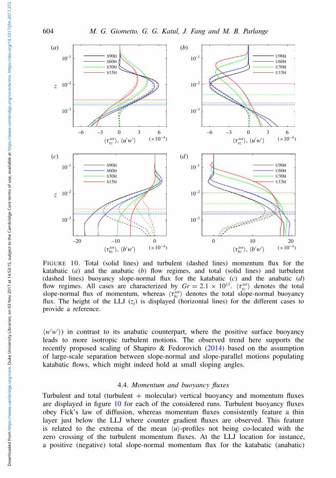
FIGURE 10. Total (solid lines) and turbulent (dashed lines) momentum flux for thekatabatic (a) and the anabatic (b) flow regimes, and total (solid lines) and turbulent(dashed lines) buoyancy slope-normal flux for the katabatic (c) and the anabatic (d)flow regimes. All cases are characterized by Gr = 2.1 × 10¹¹. 〈τ tot
xz 〉 denotes the totalslope-normal flux of momentum, whereas 〈τ tot
bz 〉 denotes the total slope-normal buoyancyflux. The height of the LLJ (zj) is displayed (horizontal lines) for the different cases toprovide a reference.
〈w′w′〉) in contrast to its anabatic counterpart, where the positive surface buoyancyleads to more isotropic turbulent motions. The observed trend here supports therecently proposed scaling of Shapiro & Fedorovich (2014) based on the assumptionof large-scale separation between slope-normal and slope-parallel motions populatingkatabatic flows, which might indeed hold at small sloping angles.
4.4. Momentum and buoyancy fluxesTurbulent and total (turbulent + molecular) vertical buoyancy and momentum fluxesare displayed in figure 10 for each of the considered runs. Turbulent buoyancy fluxesobey Fick’s law of diffusion, whereas momentum fluxes consistently feature a thinlayer just below the LLJ where counter gradient fluxes are observed. This featureis related to the extrema of the mean 〈u〉-profiles not being co-located with thezero crossing of the turbulent momentum fluxes. At the LLJ location for instance,a positive (negative) total slope-normal momentum flux for the katabatic (anabatic)
Dow
nloa
ded
from
htt
ps://
ww
w.c
ambr
idge
.org
/cor
e. D
uke
Uni
vers
ity L
ibra
ries
, on
03 N
ov 2
017
at 1
4:53
:15,
sub
ject
to th
e Ca
mbr
idge
Cor
e te
rms
of u
se, a
vaila
ble
at h
ttps
://w
ww
.cam
brid
ge.o
rg/c
ore/
term
s. h
ttps
://do
i.org
/10.
1017
/jfm
.201
7.37
2

Direct numerical simulation of turbulent slope flows 605
101
–1.0 1.0–0.5 0 0.5 –2 1–1 0
102
103(a) (b)
101
102
103S90HS60HS30HS15H
U90HU60HU30HU15H
FIGURE 11. Total (solid lines) and turbulent (dashed lines) momentum flux for thekatabatic (a) and the anabatic (b) flow regimes in inner units. All cases are characterizedby Gr= 2.1× 10¹¹. 〈τ tot
xz 〉 denotes the total slope-normal flux of momentum. The height ofthe LLJ (zj) is displayed (horizontal lines) for the different cases to provide a reference.
flow regime are observed. Note that counter gradient fluxes have been previouslyreported in experimental studies (Smeets et al. 2000; Oldroyd et al. 2016a). Thepeak magnitude of both 〈τ tot
xz 〉 and 〈τ totbz 〉 in the above-LLJ regions is dependent on
α for both flow regimes (it decreases as α decreases). In addition, katabatic flowsolutions are characterized by a modest upward shift of flux extrema as the slopingangle decreases, whereas the upward shift is more significant for the anabatic flowcases. Such trends are directly related to the combined effects of α on the scales ofthe flow (recall that the analytic Prandtl solution predicts L∝ (sin (α))−1/2) and of thesurface induced stratification in katabatic and anabatic flows, whose strength increasesas α decreases, progressively damping (for the katabatic cases) or enhancing (for theanabatic cases) turbulent fluctuations. In the FS09 study, the peak magnitude of 〈τ tot
xz 〉
and 〈τ totbz 〉 in the katabatic flow regime was found to be approximately constant and
independent of α. Conversely, it was sensitive to α in the anabatic flow cases, inapparent contrast with current findings. Such a mismatch is related to the differentsurface forcing approach that characterizes the current and the FS90 study (in FS90a constant surface buoyancy flux is applied to drive the flow).
Figure 11 features the total and the turbulent momentum fluxes for the consideredkatabatic and anabatic flow regimes in inner units. For katabatic flows the viscouscontribution to the total flux is dominant in the below-LLJ regions, and drops toless than 10 % as z+ > 50 for the α = 90◦ case. As the sloping angle decreases theviscous contribution in the above-LLJ region increases, due to the strengthening ofthe stable stratification resulting from the imposed surface buoyancy, and amounts toapproximately 35 % the total at z+ = 50 for the shallower of the considered slopes(α = 15◦). In contrast, anabatic flows are characterized by a decrease of viscouscontributions to the total momentum flux as the sloping angle decreases throughoutthe boundary layer, with viscous effects remaining dominant up to z+ ≈ 12, whereviscous and turbulent fluxes are roughly of the same magnitude, and becomingnegligible (<10 %) as z+ > 50. From figure 11 is also apparent how the surfacecontribution in terms of total stress is larger than the peak stress in the above-LLJregion for katabatic flows, whereas for anabatic flows as the sloping angle decreases
Dow
nloa
ded
from
htt
ps://
ww
w.c
ambr
idge
.org
/cor
e. D
uke
Uni
vers
ity L
ibra
ries
, on
03 N
ov 2
017
at 1
4:53
:15,
sub
ject
to th
e Ca
mbr
idge
Cor
e te
rms
of u
se, a
vaila
ble
at h
ttps
://w
ww
.cam
brid
ge.o
rg/c
ore/
term
s. h
ttps
://do
i.org
/10.
1017
/jfm
.201
7.37
2

606 M. G. Giometto, G. G. Katul, J. Fang and M. B. Parlange
2–8
–6
–4
DNSLaminar
–2
15 30 60 90 15 30 60 90
4
6
8(a) (b)
FIGURE 12. α dependence of the kinematic surface average stress τw for katabatic (a)and anabatic (b) flow cases. Simulations correspond to cases S90H, S60H, S30H, S15H andU90H, U60H, U30H, U15H for the katabatic and anabatic regimes, respectively. Predictionsfrom the Prandtl laminar solution are included for comparison (black lines).
the surface stress becomes progressively smaller when compared to the outer stresspeak.
Turbulent fluctuations contribute to the overall buoyancy flux in the below-LLJregion of katabatic flows, whereas they provide a negligible contribution to theoverall momentum flux. This latter behaviour has direct effect on the overall surfacestress, which is nearly equal to the laminar flow prediction for α > 90◦, as displayedin figure 12. Turbulent motion in the below-jet regions of katabatic flows are thus‘inactive’ from a momentum transport perspective (in the Townsend (1956) sense), butare relatively effective in vertically transporting buoyancy. To the contrary, turbulentfluctuations in the anabatic flow solution contribute to both the overall surfacebuoyancy and momentum fluxes that progressively depart from their Prandtl ‘laminarflow’ counterparts as α is reduced. An interesting feature of the considered anabaticflow simulations is the magnitude of the time- and space-averaged surface totalmomentum flux (τw), as displayed in figure 12. τw is consistently smaller than itslaminar flow prediction in the anabatic cases, and its magnitude decreases as thesloping angle is reduced. Note that such feature might be related to the relativelymodest Gr value characterizing the various runs.
4.5. The mean kinetic energy budgetThe governing equation for the time- and space-averaged velocity 〈ui〉 is readilyderived by applying Reynolds decomposition to the instantaneous flow variables (e.g.ui = 〈ui〉 + u′i) and space + time averaging (2.9). The budget equation for MKE isthen obtained by multiplying the equation for 〈ui〉 by 〈ui〉 itself. Assuming horizontalhomogeneity (∂〈·〉/∂x= ∂〈·〉/∂y= 0) and no subsidence (〈w〉 = 0) it reads
∂( 12 〈u〉〈u〉)∂t
= 〈u′w′〉∂〈u〉∂z− 〈u〉〈b〉 sin (α)−
∂( 12 〈u〉〈u
′w′〉)∂z
+Gr−1/2〈u〉∂2〈u〉∂z2
, (4.9)
Dow
nloa
ded
from
htt
ps://
ww
w.c
ambr
idge
.org
/cor
e. D
uke
Uni
vers
ity L
ibra
ries
, on
03 N
ov 2
017
at 1
4:53
:15,
sub
ject
to th
e Ca
mbr
idge
Cor
e te
rms
of u
se, a
vaila
ble
at h
ttps
://w
ww
.cam
brid
ge.o
rg/c
ore/
term
s. h
ttps
://do
i.org
/10.
1017
/jfm
.201
7.37
2

Direct numerical simulation of turbulent slope flows 607
10–3
10–2
10–1
10–3
10–2
10–1
–0.06 –0.03 0
MKE budget terms
0.03 0.06 –0.06 –0.03 0
MKE budget terms
0.03 0.06
z
(a) (b)
FIGURE 13. Slope-normal structure of the MKE budget for the katabatic (a) and forthe anabatic (b) flow regimes at α = 90◦ (solid lines), α = 60◦ (dashed lines), α = 30◦(dot-dashed lines) and α = 15◦ (dotted lines). All cases are characterized by Gr = 2.1×10¹¹. The location of the LLJ is highlighted by horizontal lines for the various runs toprovide a reference height (note that as α decreases the LLJ height increases). All termsare normalized by U3 L−1
≡ bs2
N−1.
where the left-hand side of (4.9) is the storage term of MKE, Ps ≡ 〈u′w′〉(∂〈u〉/∂z)denotes shear production/destruction of MKE, Pb ≡−〈u〉〈b〉 sin (α) denotes buoyancyproduction/destruction of MKE, transport of MKE by turbulent motions is Tt ≡
−∂(1/2〈u〉〈u′w′〉)/∂z and dissipation of MKE by viscous diffusion is E ≡ Gr−1/2〈u〉
(∂2〈u〉/∂z2). When time averaging over a sufficiently long time period then ∂〈·〉/∂t= 0
and the storage term can be neglected.The normalized MKE budget terms for the considered anabatic and katabatic
runs are displayed in figure 13. The choice of bs2N−1 as a normalizing factor is
not critical for the interpretation of the budget, since the relative magnitude of theterms is unchanged. As expected, the overall main source of MKE is from buoyancyproduction (Pb), which peaks in the below-jet regions, and is characterized by agradual decrease throughout the boundary layer. In the outer regions of the flow,Pb becomes a sink of MKE in both flow regimes starting from the zero crossingof 〈b〉 and up to the start of the return flow region. Here, energy is provided byturbulent transport (Tt), which balances shear production (Ps) and buoyant production(Pb) (both Ps and Pb are a sink term of MKE in such layer). At the wall, buoyantproduction is overcome by dissipation for both upslope and downslope flows, andtransport from turbulent motions is responsible to close the MKE budget. Tt acts asa sink of MKE in the highly energetic LLJ regions, displacing it toward the wall tobalance the enhanced dissipation, and also into the outer layer of the flow.
In both anabatic and katabatic flow regimes, shear production of MKE (Ps)acts as a sink of MKE in the above-jet regions, draining energy from the meanflow and transferring it to turbulence through the classical energy cascade process.Interestingly, for both regimes and all the considered sloping angles, the below-jetregions are characterized by Ps> 0, highlighting a region of global energy backscatter,i.e. energy is transferred from the turbulent eddies to the mean flow. Forward scatter
Dow
nloa
ded
from
htt
ps://
ww
w.c
ambr
idge
.org
/cor
e. D
uke
Uni
vers
ity L
ibra
ries
, on
03 N
ov 2
017
at 1
4:53
:15,
sub
ject
to th
e Ca
mbr
idge
Cor
e te
rms
of u
se, a
vaila
ble
at h
ttps
://w
ww
.cam
brid
ge.o
rg/c
ore/
term
s. h
ttps
://do
i.org
/10.
1017
/jfm
.201
7.37
2
608 M. G. Giometto, G. G. Katul, J. Fang and M. B. Parlange
is known to be mainly caused by vortex stretching by the mean strain rate, whereasbackscatter indicates vortex compression by the mean strain rate, which is notcommonly observed in canonical wall-bounded flows.
4.6. The turbulent kinetic energy budgetUnder the assumptions leading to (4.9), the budget equation for TKE is given as
∂〈 12 u′iu
′
i〉
∂t= −〈u′w′〉
∂〈u〉∂z+ 〈b′w′〉 cos (α)− 〈b′u′〉 sin (α)−
∂〈 12 u′iu
′
iw′〉
∂z
−∂〈π′w′〉∂z
+Gr−1/2 ∂2〈
12 u′iu
′
i〉
∂z2−Gr−1/2
⟨∂u′i∂xj
∂u′i∂xj
⟩, (4.10)
where ∂〈(1/2)u′iu′
i〉/∂t is the storage of TKE term, shear production of TKEis denoted as Ps ≡ −〈u′w′〉(∂〈u〉/∂z), buoyant production/destruction of TKE iscomposed of two terms, namely Pb,1≡ 〈b′u′〉 sin(α) and Pb,3≡ 〈b′w′〉 cos(α), turbulenttransport of TKE is Tt ≡ −∂〈(1/2)u′iu
′
iw′〉/∂z, pressure transport Tp ≡ −∂〈π
′w′〉/∂z,viscous diffusion of TKE is Tν ≡ Gr−1/2∂2
〈(1/2)u′iu′
i〉/∂z2 and viscous dissipationε ≡ −Gr−1/2
〈(∂u′i/∂xj)(∂u′i/∂xj)〉. With regard to the buoyancy production/destructionterms, Pb,1 accounts for production/destruction of TKE due to cross-correlationbetween along-slope velocity (u) and buoyancy (b), whereas Pb,3 accounts forproduction/destruction of TKE due to cross-correlation between normal-to-slopevelocity (w) and buoyancy (b). The splitting of the buoyancy production term isclearly a result of the inclined reference system that is adopted to describe theevolution of the system.
TKE budget terms for the considered runs (characterized by Gr = 2.1 × 10¹¹) aredisplayed in figure 14. Shear production (Ps) appears with opposite signs in thebudgets of MKE and TKE as expected. It represents the net transfer from MKEto TKE as the result of their interactions that often sustains turbulence in classicalboundary layer theory on flat slopes. For both anabatic and katabatic flow regimes,Ps is characterized by two positive peaks, one in the above jet regions and one inthe very near-wall regions, and is negative in a small interval just below the LLJ,where global energy backscatter occurs. Occurrence of negative Ps is related tothe presence of local (in z) counter-gradient turbulent momentum flux, in line withfindings of § 4.4. In both katabatic and anabatic flow regimes, ε peaks at the wall, isapproximately constant in the near-LLJ region and decreases logarithmically in thecore of the flow. The Pb,3 is a sink of TKE for the katabatic regime and a source ofTKE for the anabatic regime, as expected. In the anabatic regime Pb,3= 0 at α= 90◦,but gains considerable importance (as a TKE source term) in the overall budgetas α decreases. For instance, considering the α = 15◦ run, Pb,3 alone overcomesTKE dissipation in the core of the LLJ. To the contrary, the modest magnitudeof Pb,3 highlights how buoyant destruction of TKE is not the primary mechanismthrough which buoyancy acts to suppress turbulence in katabatic flows. Following thesame reasoning of Shah & Bou-Zeid (2014) (where stability effects on the Ekmanlayer were studied through DNS), it is argued here that negative buoyancy directlyreduces 〈w′w′〉, thus reducing local production of 〈u′w′〉. A reduction in 〈u′w′〉 wouldultimately result in the observed decrease in 〈Ps〉 and related TKE magnitude as αdecreases (i.e. as the static stability of the environment increases). Pb,1 is the majorsource of TKE at the LLJ for the katabatic flow regime at all the considered α.On the other hand, in the anabatic flow regime Pb,3 overcomes Pb,1 as α decreases,
Dow
nloa
ded
from
htt
ps://
ww
w.c
ambr
idge
.org
/cor
e. D
uke
Uni
vers
ity L
ibra
ries
, on
03 N
ov 2
017
at 1
4:53
:15,
sub
ject
to th
e Ca
mbr
idge
Cor
e te
rms
of u
se, a
vaila
ble
at h
ttps
://w
ww
.cam
brid
ge.o
rg/c
ore/
term
s. h
ttps
://do
i.org
/10.
1017
/jfm
.201
7.37
2
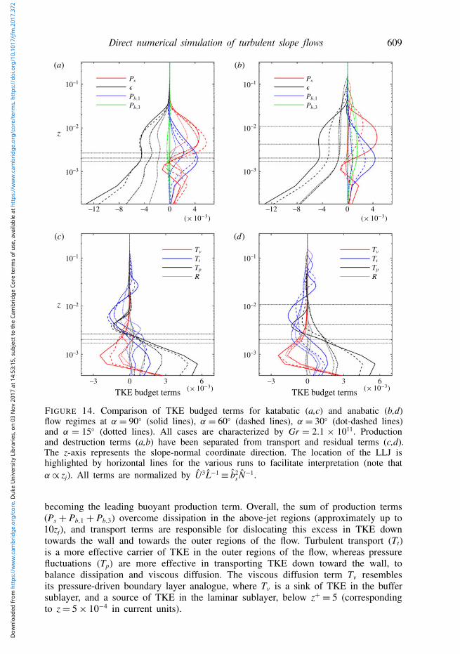
Direct numerical simulation of turbulent slope flows 609
10–3
–12 –8 –4
z
z
0 4
10–2
10–1
(a) (b)
(c) (d)
10–3
–12 –8 –4 0 4
10–2
10–1
10–3
–3 0 3
TKE budget terms6 –3 0 3 6
10–2
10–1
10–3
TKE budget terms
10–2
10–1
FIGURE 14. Comparison of TKE budged terms for katabatic (a,c) and anabatic (b,d)flow regimes at α = 90◦ (solid lines), α = 60◦ (dashed lines), α = 30◦ (dot-dashed lines)and α = 15◦ (dotted lines). All cases are characterized by Gr = 2.1 × 10¹¹. Productionand destruction terms (a,b) have been separated from transport and residual terms (c,d).The z-axis represents the slope-normal coordinate direction. The location of the LLJ ishighlighted by horizontal lines for the various runs to facilitate interpretation (note thatα ∝ zj). All terms are normalized by U3L−1
≡ b2s N−1.
becoming the leading buoyant production term. Overall, the sum of production terms(Ps + Pb,1 + Pb,3) overcome dissipation in the above-jet regions (approximately up to10zj), and transport terms are responsible for dislocating this excess in TKE downtowards the wall and towards the outer regions of the flow. Turbulent transport (Tt)is a more effective carrier of TKE in the outer regions of the flow, whereas pressurefluctuations (Tp) are more effective in transporting TKE down toward the wall, tobalance dissipation and viscous diffusion. The viscous diffusion term Tν resemblesits pressure-driven boundary layer analogue, where Tν is a sink of TKE in the buffersublayer, and a source of TKE in the laminar sublayer, below z+ = 5 (correspondingto z= 5× 10⁻⁴ in current units).
Dow
nloa
ded
from
htt
ps://
ww
w.c
ambr
idge
.org
/cor
e. D
uke
Uni
vers
ity L
ibra
ries
, on
03 N
ov 2
017
at 1
4:53
:15,
sub
ject
to th
e Ca
mbr
idge
Cor
e te
rms
of u
se, a
vaila
ble
at h
ttps
://w
ww
.cam
brid
ge.o
rg/c
ore/
term
s. h
ttps
://do
i.org
/10.
1017
/jfm
.201
7.37
2

610 M. G. Giometto, G. G. Katul, J. Fang and M. B. Parlange
10–3
–8 –4 0 4 –8 –4 0 4
10–2z
10–1
(a)
10–3
10–2
10–1
(b)
FIGURE 15. Comparison of return-to-isotropy terms for katabatic (a) and anabatic (b) flowregimes at Gr = 2.1 × 10¹¹. We denote Φ1 ≡ 〈p′(∂u′/∂x)〉, Φ2 ≡ 〈p′(∂v′/∂y)〉 and Φ3 ≡
〈p′(∂w′/∂z)〉. The location of the LLJ is once again highlighted with horizontal lines andthe α = 90◦, 60◦, 30◦ and 15◦ runs (simulations S90H, S60H, S30H, S15H for the katabaticregimes; U90H, U60H, U30H, U15H for the anabatic regimes) are denoted with solid, dashed,dot-dashed and dotted lines respectively. The z-axis represents the slope-normal coordinatedirection and all terms are normalized by U3 L−1
≡ b2s N−1.
Not shown here is the vertical structure of flux Richardson number (Rif =
〈b′w′〉/(d〈u〉/dz)〈u′w′〉), which is positive (negative) throughout the core of theboundary layer (above the LLJ and below the return flow region) in the katabatic(anabatic) flow regimes. In the katabatic flow regime Rif is lower in magnitudethan its critical value of 0.25, except in the neighbourhood of the LLJ the stablestratification and low velocity gradients result instead in Rif � 1.
It is worth noting the significant contribution of turbulent and pressure transportterms in the neighbourhood of the LLJ and in the wall regions in both flowregimes. Pressure fluctuations are relevant in the near-wall regions when comparedto corresponding values observed in neutral (Moser, Kim & Moin 1999) and stablystratified (Iida, Kasagi & Nagano 2002) pressure-driven channel flow DNS. In theneighbourhood of the LLJ Rif is relatively large in magnitude (not shown) for bothflow regimes, promoting strong internal gravity wave activity, which does not transferbuoyancy, but can be effective in transporting momentum through the action ofpressure force, thus justifying such relevant contribution of pressure transport to theTKE budget.
The return-to-isotropy term (also known as pressure redistribution term) contractsto zero, and so vanishes from the TKE budget equation (4.10). However, whenanalysed for the single TKE budget components displayed in figure 15, the role ofturbulence in distributing turbulent energy becomes clear. For instance, wall dampingeffects on slope-normal velocity fluctuations are apparent in the below-LLJ regions,where Φ3 < 0 indicating energy redistribution from the slope-normal component(〈w′w′〉) to the horizontal components (〈u′u′〉 and 〈v′v′〉 respectively). In the above-jetregions for the katabatic flow regime, a consistent energy redistribution among theTKE components are observed across the sloping angles with energy being transferredfrom the streamwise component (〈u′u′〉) to the spanwise and slope-normal components
Dow
nloa
ded
from
htt
ps://
ww
w.c
ambr
idge
.org
/cor
e. D
uke
Uni
vers
ity L
ibra
ries
, on
03 N
ov 2
017
at 1
4:53
:15,
sub
ject
to th
e Ca
mbr
idge
Cor
e te
rms
of u
se, a
vaila
ble
at h
ttps
://w
ww
.cam
brid
ge.o
rg/c
ore/
term
s. h
ttps
://do
i.org
/10.
1017
/jfm
.201
7.37
2

Direct numerical simulation of turbulent slope flows 611
(〈v′v′〉 and 〈w′w′〉 respectively). For the anabatic flow regime, the return-to-isotropyterms in the above-jet regions highlight a transition in the system as a functionof α. When the two highest sloping angles are considered (α = 60◦ and α = 90◦),energy transfer is qualitatively equivalent to that characterizing the katabatic flowregime, i.e. the streamwise variance feeds the spanwise and slope-normal variancecomponents. For α = 15◦ and α = 30◦, the return-to-isotropy term becomes a sinkfor 〈w′w′〉 and a source for 〈u′u′〉 and 〈v′v′〉, indicative of energy transfer from theslope-normal TKE component to the streamwise and spanwise TKE components. Thistransition suggests that at low sloping angles, anabatic flow regimes are characterizedby slope-normal elongated eddies as apparent from figure 5, which feed 〈u′u′〉 and〈v′v′〉 from 〈w′w′〉, the latter being directly sustained by the slope-normal projectionof the buoyancy force b cos (α). Conversely, katabatic flow eddies are streamwiseelongated and remove energy from 〈u′u′〉 – directly fed by the streamwise componentof the buoyancy force – to transfer it to 〈w′w′〉 and 〈v′v′〉. This energy redistributionterm ensures some self-preservation of the slope-normal velocity variance in katabaticflows despite the adverse role of stability.
Overall, the proposed TKE budget analysis suggests a subdivision of the boundarylayer into four distinct regions, for the considered α- and Gr-ranges, namely
(i) an outer layer, corresponding approximately to the return flow region, whereturbulent transport (Tt) is the main source of TKE and balances dissipation (ε);
(ii) an intermediate layer, bounded below by the LLJ and capped above by theouter layer, where the sum of shear and buoyant production (Ps + Pb,1 + Pb,3)overcomes dissipation (ε), and where turbulent and pressure transport terms(Tt, Tp) are a sink of TKE;
(iii) a buffer layer, corresponding to 5/ z+/ 30, where TKE is provided by turbulentand pressure transport terms, to balance viscous diffusion and dissipation;
(iv) a laminar sublayer, corresponding to z+ / 5, where the influence of viscosity issignificant and the flow is approximately laminar.
5. Summary and conclusions
DNS are used to characterize mean flow and turbulence of thermally drivenflows along a uniformly cooled or heated sloping plate immersed within a stablystratified environment, using a set-up resembling the one considered by Prandtl’sslope-flow model. The study focused on sensitivity of the flow statistics to variationsin the sloping angle (α) and Grashof number (Gr) for a fixed molecular Prandtlnumber (Pr= 1). Four sloping angles (α = 15◦, 30◦, 60◦ and 90◦) and three Grashofnumber (Gr = 5× 10¹⁰, Gr = 1× 10¹¹, and Gr = 2.1× 10¹¹) were considered, whereGr = b4
s ν−2N−6 is interpreted as the ratio between the energy production at the
surface and the work against the background stratification and viscous forces. Thestudy complements the Fedorovich & Shapiro (2009) analysis, where a similar rangeof sloping angle and Gr was considered but where the flow was forced using aconstant surface buoyancy flux.
The initial transient is characterized by slowly decaying quasi-stationary oscillatorypatterns in the spatially integrated variables, the normalized oscillation frequency beingproportional to the sine of the sloping angle, in agreement with field observations ofslope flows (e.g. Princevac et al. 2008; Monti et al. 2014) and with findings from arecent theoretical work (Fedorovich & Shapiro 2017). The quality of the averagingoperation has been tested against a dynamic and an energy identity derived from the
Dow
nloa
ded
from
htt
ps://
ww
w.c
ambr
idge
.org
/cor
e. D
uke
Uni
vers
ity L
ibra
ries
, on
03 N
ov 2
017
at 1
4:53
:15,
sub
ject
to th
e Ca
mbr
idge
Cor
e te
rms
of u
se, a
vaila
ble
at h
ttps
://w
ww
.cam
brid
ge.o
rg/c
ore/
term
s. h
ttps
://do
i.org
/10.
1017
/jfm
.201
7.37
2

612 M. G. Giometto, G. G. Katul, J. Fang and M. B. Parlange
10–3
–0.2 –0.1 0 0.1 0.2 –1.0 –0.5 0 0.5 1.0
10–2z
10–1
10–3
10–2
10–1
(a) (b)
S60HS60MS60LU60HU60MU60L
FIGURE 16. Sensitivity of the streamwise velocity 〈u〉 (a) and buoyancy 〈b〉 (b) on the Grparameter, for katabatic (solid lines) and anabatic (dashed lines) flow regimes at α= 60◦.
equations of motions, that the time-averaged solution must satisfy in coordinates ofstatistical homogeneity.
With respect to their basic features, the katabatic and anabatic mean flow appearsimilar to their corresponding laminar (Prandtl) counterparts. The thermal boundarylayer is much shallower when compared to the dynamic boundary layer, the latterbeing characterized by a low-level jet near the wall regions, and by a weak returnflow in the outer regions. Turbulent anabatic and katabatic regimes are found to bestructurally similar at high sloping angles but to undergo a different transition in theturbulence production and transport mechanisms as the sloping angle decreases. Infact, a stark statistical difference between the two flow regimes for the α/ 30◦ rangewas noted from the DNS analysis. As α decreases, the negative surface buoyancydriving downslope flows leads to the formation of a strong surface inversion layer,resulting in a progressive laminarization of the solution in the near-LLJ regions. Italso results in small variation in the integrated horizontal momentum flux and in anoverall small variability of mean profiles with respect to α. Anabatic flows on theother hand are characterized by a strengthening of TKE production and turbulentmomentum fluxes as α decreases, by a significant α dependence of the overallhorizontal momentum flux, and by well mixed profiles of buoyancy and velocity,suggesting the presence of convective cells for α/ 30◦. Analysis of the slope-normalintegrated energy equation highlights how the characteristic (normalized) scale ofanabatic flow L∝ 1/sinα, whereas the characteristic scale of katabatic flow is foundto be poorly sensitive to α. As in Fedorovich & Shapiro (2009), no region withconstancy (even approximate) of any of the fluxes with distance from the wall hasbeen identified, and molecular diffusion of momentum and buoyancy are found to besignificant in the below-LLJ regions, when compared to turbulent diffusion. Budgetequations show how MKE is fed into the fluid system through the imposed surfacebuoyancy, and turbulent fluctuations redistribute it from the lower edge of the jettoward the wall and toward the outer layer. Interestingly, as Gr increases, the overallnormalized energy of the system is reduced, but turbulent fluctuations gain importancein the below-jet regions. Hence, despite the modest Grashof number range consideredhere, one might speculate about the existence of a (turbulent) overlap layer at higher
Dow
nloa
ded
from
htt
ps://
ww
w.c
ambr
idge
.org
/cor
e. D
uke
Uni
vers
ity L
ibra
ries
, on
03 N
ov 2
017
at 1
4:53
:15,
sub
ject
to th
e Ca
mbr
idge
Cor
e te
rms
of u
se, a
vaila
ble
at h
ttps
://w
ww
.cam
brid
ge.o
rg/c
ore/
term
s. h
ttps
://do
i.org
/10.
1017
/jfm
.201
7.37
2

Direct numerical simulation of turbulent slope flows 613
1.5
0.5 1.0
Gr Gr1.5 2.0 0.5 1.0 1.5 2.0
4
5
6
7
8
9
10
2.0
2.5
(a) (b)
FIGURE 17. Absolute value of the averaged surface buoyancy flux (a) and momentum flux(b) as a function of Gr for anabatic (red line) and katabatic (black line) flow regimes atα = 60◦ (simulations S60H, S60M, S60L and U60H, U60M, U60L, respectively).
Gr, located in the below-jet region, separating the LLJ from the laminar sublayer.In addition, a zone of global backscatter (energy transfer from the turbulent eddiesto the mean flow) is consistently found just below the LLJ, which highlights thepresence of vortex compression (instead of stretching) dynamical mechanisms, andfailure of gradient diffusion theory in such layer. The behaviour in returning toisotropy of turbulent fluctuations further highlights how katabatic and anabatic flowsystems differ in their mechanisms sustaining turbulence at shallow slopes, and againindicates presence of convective cells for α/ 30◦ in anabatic flows. Overall, analysisof the α dependence of the TKE budget terms suggests a subdivision of the boundarylayer in four distinct regions: (i) an outer layer, approximately corresponding to thereturn flow region, where turbulent transport balances dissipation, (ii) an intermediatelayer, bounded below by the LLJ, where shear and buoyant production overcomedissipation, and turbulent and pressure fluctuations are responsible to relocate theexcess TKE down toward the wall and toward the outer layer, (iii) a buffer layer,capped above by the LLJ, where pressure and turbulent transport balance dissipationand viscous diffusion of TKE and (iv) a laminar sublayer, where molecular viscosityand thermal diffusivity effects are of leading order in the transport of momentum andbuoyancy.
The proposed DNS results, in particular the TKE and MKE budgets, and the role ofturbulence isotropization via pressure fluctuations can be used to guide improvementsin current turbulence closure modelling for sloping and stable conditions that can thenbe implemented in the next generation of large-scale atmospheric models.
Appendix A. Sensitivity of solutions to variations in the Grashof numberA.1. Mean flow, TKE and buoyancy variance
The sensitivity of mean velocity and buoyancy profiles to variations in Gr is displayedin figure 16 for anabatic and katabatic flow regimes characterized by α = 60◦.Increases in Gr results in weaker thermal and dynamic boundary layers, i.e. in a
Dow
nloa
ded
from
htt
ps://
ww
w.c
ambr
idge
.org
/cor
e. D
uke
Uni
vers
ity L
ibra
ries
, on
03 N
ov 2
017
at 1
4:53
:15,
sub
ject
to th
e Ca
mbr
idge
Cor
e te
rms
of u
se, a
vaila
ble
at h
ttps
://w
ww
.cam
brid
ge.o
rg/c
ore/
term
s. h
ttps
://do
i.org
/10.
1017
/jfm
.201
7.37
2

614 M. G. Giometto, G. G. Katul, J. Fang and M. B. Parlange
10–3
0 0 0.015 0.030 0.0451 2 3
10–2z
10–1
(a) (b)
10–3
10–2
10–1S60HS60MS60LU60HU60MU60L
FIGURE 18. Sensitivity of the turbulent kinetic energy ((1/2)〈u′iu′
i〉) (a) and buoyancyvariance (〈b′b′〉) (b) to the Gr parameter for katabatic (solid lines) and anabatic (dashedlines) flow regimes at α = 60◦.
1
10–3
10–2
10–1
–0.06 –0.03 0
MKE budget terms
0.03 0.06 –0.06 –0.03 0
MKE budget terms
0.03 0.06
2
3
4
5z
6
7
8
9(a) (b)
FIGURE 19. Sensitivity of MKE budget terms to Gr for the katabatic (a) and the anabatic(b) flow regimes at α = 60◦. Profiles correspond to Gr = 1 × 10¹⁰ (dot-dashed lines),Gr= 5× 10¹¹ (dashed lines) and Gr= 2.1× 10¹¹ (solid lines). The location of the LLJ ishighlighted with horizontal dotted black lines for the various runs, to provide a referenceheight (note that as Gr increases the LLJ height decreases). All terms are normalized byU3 L−1
≡ bs2
N−1.
decrease of zj, uj, δ, as well as∫ H
0 〈b〉 dz and∫ H
0 〈u〉 dz. As apparent from figure 17,increases in Gr results in a decrease in the surface buoyancy flux 〈τbz〉|z=0, i.e. ina reduction of the rate of potential energy that is supplied to the system, as couldhave been intuitively predicted. Surface momentum fluxes are also decreasing as Grincreases, as also displayed in figure 17. Conversely, the magnitude of slope-normalsurface gradients of along-slope velocity and buoyancy are stronger as Gr increases,
Dow
nloa
ded
from
htt
ps://
ww
w.c
ambr
idge
.org
/cor
e. D
uke
Uni
vers
ity L
ibra
ries
, on
03 N
ov 2
017
at 1
4:53
:15,
sub
ject
to th
e Ca
mbr
idge
Cor
e te
rms
of u
se, a
vaila
ble
at h
ttps
://w
ww
.cam
brid
ge.o
rg/c
ore/
term
s. h
ttps
://do
i.org
/10.
1017
/jfm
.201
7.37
2

Direct numerical simulation of turbulent slope flows 615
10–3
–12 –8 –4
z
z
0 4
10–2
10–1
(a) (b)
(c) (d)
10–3
–12 –8 –4 0 4
10–2
10–1
10–3
–3 0 3
TKE budget terms6 –3 0 3 6
10–2
10–1
10–3
TKE budget terms
10–2
10–1
FIGURE 20. Sensitivity of TKE budget terms to Gr for the katabatic (a,c) and the anabatic(b,d) flow regimes at α = 60◦. Profiles correspond to Gr = 5 × 10¹⁰ (dot-dashed lines),Gr= 1× 10¹¹ (dashed lines), and Gr= 2.1× 10¹¹ (solid lines). The z-axis represents theslope-normal coordinate direction. The location of the LLJ is highlighted with dotted blacklines for the various runs, to provide a reference height (note that as Gr increases the LLJheight decreases). All terms are normalized by U3 L−1
≡ bs2
N−1.
highlighting a relatively stronger momentum (buoyancy) replenishment (extraction)induced by turbulent fluctuations. Therefore as Gr increases, the LLJ becomes weakerbut better mixed.
The relatively stronger role of turbulent fluctuations in the near-wall regions as Grincreases is apparent if one focuses on figure 18, where TKE and buoyancy varianceare featured for both flow regimes. Higher Gr results in stronger near-wall TKE and〈b′b′〉, despite the relatively lower kinetic and potential energy of the system, whencompared to the same simulation at lower Gr. Worth noting also how the near-surfacepeak of 〈b′b′〉 is insensitive to Gr. This behaviour is in line with findings from meanprofiles, which suggest a stronger role of turbulent fluctuations in the near-wall regionas Gr increases. In the above-LLJ regions TKE, 〈b′b′〉 and the slope-normal scale of
Dow
nloa
ded
from
htt
ps://
ww
w.c
ambr
idge
.org
/cor
e. D
uke
Uni
vers
ity L
ibra
ries
, on
03 N
ov 2
017
at 1
4:53
:15,
sub
ject
to th
e Ca
mbr
idge
Cor
e te
rms
of u
se, a
vaila
ble
at h
ttps
://w
ww
.cam
brid
ge.o
rg/c
ore/
term
s. h
ttps
://do
i.org
/10.
1017
/jfm
.201
7.37
2

616 M. G. Giometto, G. G. Katul, J. Fang and M. B. Parlange
the flow increase in magnitude as Gr is reduced for all the considered cases, likelydue to the relatively stronger dynamic and thermal boundary layers.
A.2. MKE and TKE budget termsThe dependence of MKE budget terms on Gr is highlighted in figure 19. Besides theexpected decrease in the slope-normal scale as Gr increases, one of the main featuresof the MKE budget terms is a relative strengthening of Ps and Tt in the below-LLJregions as Gr increases. With this regard, note how the peak value of Pb and εs aresensitive to variations in Gr, whereas the peak value of Ps and Tt are insensitiveto Gr.
As Gr increases, TKE budget terms are characterized by a strengthening of Ps inthe neighbourhood of the LLJ and near-surface regions for the katabatic flow regimes(see figure 20). Anabatic flows are instead characterized by a strengthening of Ps inthe near-wall regions, well below zj. In addition, buoyant production Pb,1 increasesas Gr increases in the below LLJ regions and transport terms tend to decrease. Thissuggests that at higher Gr when compared to those considered herein, anabatic andkatabatic flows might be characterized by a relatively important local TKE productionrate in the below-LLJ regions, and negligible TKE transport rates, ultimately resultingin stronger TKE, and thus larger zj and well-mixed profiles of buoyancy and velocity.Such a region might well be the equivalent of the overlap (logarithmic) layer incanonical wall-bounded turbulent flows, which is not observed here, probably becauseof the relatively low Gr values.
REFERENCES
ABKAR, M., BAE, H. J. & MOIN, P. 2016 Minimum-dissipation scalar transport model for large-eddysimulation of turbulent flows. Phys. Rev. Fluids 1 (4), 041701.
ALBERTSON, J. D. & PARLANGE, M. B. 1999a Natural integration of scalar fluxes from complexterrain. Adv. Water Resour. 23 (3), 239–252.
ALBERTSON, J. D. & PARLANGE, M. B. 1999b Surface length scales and shear stress: implicationsfor land-atmosphere interaction over complex terrain. Water Resour. Res. 35 (7), 2121–2132.
ARDUINI, G., STAQUET, C. & CHEMEL, C. 2016 Interactions between the nighttime valley-windsystem and a developing cold-air pool. Boundary-Layer Meteorol 161 (1), 49–72.
AXELSEN, S. & DOP, H. 2009a Large-eddy simulation of katabatic winds. Part 1: comparison withobservations. Acta Geophys. 57 (4), 803–836.
AXELSEN, S. L. & DOP, H. 2009b Large-eddy simulation of katabatic winds. Part 2: sensitivitystudy and comparison with analytical models. Acta Geophys. 57 (4), 837–856.
BOU-ZEID, E., MENEVEAU, C. & PARLANGE, M. B. 2005 A scale-dependent Lagrangian dynamicmodel for large eddy simulation of complex turbulent flows. Phys. Fluids 17 (2), 025105.
BOU-ZEID, E., OVERNEY, J., ROGERS, B. D. & PARLANGE, M. B. 2009 The effects of buildingrepresentation and clustering in large-eddy simulations of flows in urban canopies. Boundary-Layer Meteorol. 132 (3), 415–436.
BURKHOLDER, B., FEDOROVICH, E. & SHAPIRO, A. 2011 Evaluating subgrid-scale models forlarge-eddy simulation of turbulent katabatic flow. In Qual Reliab Large-eddy Simulations II,pp. 149–160. Springer.
BURKHOLDER, B., SHAPIRO, A. & FEDOROVICH, E. 2009 Katabatic flow induced by a cross-slopeband of surface cooling. Acta Geophys. 57 (4), 923–949.
BURNS, P. & CHEMEL, C. 2014 Evolution of cold-air-pooling processes in complex terrain. Boundary-Layer Meteorol. 150 (3), 423–447.
BURNS, P. & CHEMEL, C. 2015 Interactions between downslope flows and a developing cold-airpool. Boundary-Layer Meteorol. 154 (1), 57–80.
Dow
nloa
ded
from
htt
ps://
ww
w.c
ambr
idge
.org
/cor
e. D
uke
Uni
vers
ity L
ibra
ries
, on
03 N
ov 2
017
at 1
4:53
:15,
sub
ject
to th
e Ca
mbr
idge
Cor
e te
rms
of u
se, a
vaila
ble
at h
ttps
://w
ww
.cam
brid
ge.o
rg/c
ore/
term
s. h
ttps
://do
i.org
/10.
1017
/jfm
.201
7.37
2

Direct numerical simulation of turbulent slope flows 617
CALAF, M., MENEVEAU, C. & MEYERS, J. 2010 Large eddy simulation study of fully developedwind-turbine array boundary layers. Phys. Fluids 22 (1), 015110.
CALAF, M., PARLANGE, M. B. & MENEVEAU, C. 2011 Large eddy simulation study of scalartransport in fully developed wind-turbine array boundary layers. Phys. Fluids 23 (12), 126603.
CANUTO, C., HUSSAINI, M. Y., QUARTERONI, A. & ZANG, T. A. 2006 Spectral Methods. Springer.CHAMECKI, M., MENEVEAU, C. & PARLANGE, M. B. 2009 Large eddy simulation of pollen transport
in the atmospheric boundary layer. J. Aero. Sci. 40, 241–255.CHEMEL, C., STAQUET, C. & LARGERON, Y. 2009 Generation of internal gravity waves by a katabatic
wind in an idealized alpine valley. Meteorol. Atmos. Phys. 103 (1–4), 187–194.CHORIN, A. J. 1968 Numerical solution of the Navier–Stokes equations. Math. Comput. 22 (104),
745–762.CHOW, F. K., WEIGEL, A. P., STREET, R. L., ROTACH, M. W. & XUE, M. 2006 High-resolution
large-eddy simulations of flow in a steep Alpine valley. Part I: Methodology, verification, andsensitivity experiments. J. Appl. Meteorol. Climatol. 45 (1), 63–86.
CHU, P. C. 1987 An instability theory of ice-air interaction for the formation of ice edge bands.J. Geophys. Res. 92 (C7), 6966–6970.
DEFANT, F. 1949 Zur theorie der hangwinde, nebst bemerkungen zur theorie der berg- und talwinde.Arch. Meteorol. Geophys. Bioklimatol. Ser A 1, 421–450.
DENBY, B. 1999 Second-order modelling of turbulence in katabatic flows. Boundary-Layer Meteorol.92 (1), 65–98.
DORAN, J. C. & HORST, T. W. 1981 Velocity and temperature oscillations in drainage winds. J. Appl.Meteorol. 20 (4), 361–364.
EGGER, J. 1985 Slope winds and the axisymmetric circulation over Antarctica. J. Atmos. Sci. 42(17), 1859–1867.
FEDOROVICH, E. & SHAPIRO, A. 2009 Structure of numerically simulated katabatic and anabaticflows along steep slopes. Acta Geophys. 57 (4), 981–1010.
FEDOROVICH, E. & SHAPIRO, A. 2017 Oscillations in Prandtl slope flow started from rest. Q. J. R.Meteorol. Soc. 143 (703), 670–677.
FERNANDO, H. J. S. 2010 Fluid dynamics of urban atmospheres in complex terrain. Annu. Rev.Fluid Mech. 42 (1), 365–389.
FERNANDO, H. J. S., PARDYJAK, E. R, DI SABATINO, S., CHOW, F. K., DE WEKKER, S. F.,HOCH, S. W., HACKER, J., PACE, J. C., PRATT, T., PU, Z. et al. 2015 The MATERHORN:Unraveling the intricacies of mountain weather. Bull. Am. Meteorol. Soc. 96 (11), 1945–1967.
GIOMETTO, M. G., CHRISTEN, A., MENEVEAU, C., FANG, J., KRAFCZYK, M. & PARLANGE, M.B. 2016 Spatial characteristics of roughness sublayer mean flow and turbulence over a realisticurban surface. Boundary-Layer Meteorol. 160 (3), 425–452.
GIOMETTO, M. G., GRANDI, R., FANG, J., MONKEWITZ, P. A. & PARLANGE, M. B. 2017 Katabaticflow: a closed-form solution with spatially-varying eddy diffusivities. Boundary-Layer Meteorol162 (2), 307–317.
GRACHEV, A. A., LEO, L. S., SABATINO, S. D., FERNANDO, H. J. S., PARDYJAK, E. R. &FAIRALL, C. W. 2016 Structure of turbulence in katabatic flows below and above the wind-speed maximum. Boundary-Layer Meteorol. 159 (3), 469–494.
GREUELL, J. W., BROEKE VAN DEN, M. R., KNAP, W., REIJMER, C., SMEETS, P. & STRUIJK,I. 1994 PASTEX: a glacio-meteorological experiment on the Pasterze (Austria). Tech. Rep.,Institute for Marine and Atmospheric Research, University, Utrecht.
GRISOGONO, B. & AXELSEN, S. L. 2012 A note on the pure katabatic wind maximum over gentleslopes. Boundary-Layer Meteorol. 145 (3), 527–538.
GRISOGONO, B., JURLINA, T., VECENAJ, Ž. & GÜTTLER, I. 2014 Weakly nonlinear Prandtl modelfor simple slope flows. Q. J. R. Meteorol. Soc. 141, 883–892.
GRISOGONO, B., KRALJEVIC, L. & JERICEVIC, A. 2007 The low-level katabatic jet height versusMonin Obukhov height. Q. J. R. Meteorol. Soc. 133, 2133–2136.
GRISOGONO, B. & OERLEMANS, J. 2001a A theory for the estimation of surface fluxes in simplekatabatic flows. Q. J. R. Meteorol. Soc. 127, 2725–2739.
Dow
nloa
ded
from
htt
ps://
ww
w.c
ambr
idge
.org
/cor
e. D
uke
Uni
vers
ity L
ibra
ries
, on
03 N
ov 2
017
at 1
4:53
:15,
sub
ject
to th
e Ca
mbr
idge
Cor
e te
rms
of u
se, a
vaila
ble
at h
ttps
://w
ww
.cam
brid
ge.o
rg/c
ore/
term
s. h
ttps
://do
i.org
/10.
1017
/jfm
.201
7.37
2

618 M. G. Giometto, G. G. Katul, J. Fang and M. B. Parlange
GRISOGONO, B & OERLEMANS, J 2001b Katabatic flow: analytic solution for gradually varying eddydiffusivities. J. Atmos. Sci. 58 (21), 3349–3354.
GRISOGONO, B. & OERLEMANS, J. 2002 Justifying the WKB approximation in pure katabatic flows.Tellus 54 (5), 453–462.
GUTMAN, L. N. 1983 On the theory of the katabatic slope wind. Tellus 35A, 213–218.GÜTTLER, I., MARINOVIC, I., VECENAJ, Ž & GRISOGONO, B. 2016 Energetics of slope flows: linear
and weakly nonlinear solutions of the extended Prandtl model. Front. Earth Sci. 4 (July),1–13.
HAIDEN, T. & WHITEMAN, C. D. 2005 Katabatic flow mechanisms on a low-angle slope. J. Appl.Meteorol. 44 (1), 113–126.
HANG, C., NADEAU, D. F., GULTEPE, I., HOCH, S. W., ROMÁN-CASCÓN, C., PRYOR, K.,FERNANDO, H. J. S., CREEGAN, E. D., LEO, L. S. & SILVER, Z. 2016 A case studyof the mechanisms modulating the evolution of valley fog. Pure Appl. Geophys. 173 (9),1–20.
HIGGINS, C. W., PARLANGE, M. B. & MENEVEAU, C. 2003 Alignment trends of velocity gradientsand subgrid-scale fluxes in the turbulent atmospheric boundary layer. Boundary-Layer Meteorol.109 (1), 59–83.
HULTMARK, M., CALAF, M. & PARLANGE, M. B. 2013 A new wall shear stress model foratmospheric boundary layer simulations. J. Atmos. Sci. 70 (11), 3460–3470.
IIDA, O., KASAGI, N. & NAGANO, Y. 2002 Direct numerical simulation of turbulent channel flowunder stable density stratification. Intl J. Heat Mass Transfer 45, 1693–1703.
ISRAELI, M. & ORSZAG, S. A. 1981 Approximation of radiation boundary conditions. J. Comput.Phys. 41 (1), 115–135.
JENSEN, D. D., NADEAU, D. F., HOCH, S. W. & PARDYJAK, E. R. 2016 Observations of near-surfaceheat-flux and temperature profiles through the early evening transition over contrasting surfaces.Boundary-Layer Meteorol. 159 (3), 567–587.
KAVAVCIC, I. & GRISOGONO, B. 2007 Katabatic flow with Coriolis effect and gradually varyingeddy diffusivity. Boundary-Layer Meteorol. 125 (2), 377–387.
KRAVCHENKO, A. G. G. & MOIN, P. 1997 On the effect of numerical errors in large eddy simulationsof turbulent flows. J. Comput. Phys. 131 (2), 310–322.
KUMAR, V., KLEISSL, J., MENEVEAU, C. & PARLANGE, M. B. 2006 Large-eddy simulation of adiurnal cycle of theatmospheric boundary layer: atmospheric stabilityand scaling issues. WaterResour. Res. 42, W06D09.
LEHNER, M., WHITEMAN, C. D., HOCH, S. W., JENSEN, D., PARDYJAK, E. R., LEO, L. S.,DI SABATINO, S. & FERNANDO, H. J. S. 2015 A case study of the nocturnal boundarylayer evolution on a slope at the foot of a desert mountain. J. Appl. Meteorol. Climatol. 54(4), 732–751.
LU, H. & PORTÉ-AGEL, F. 2010 A modulated gradient model for large-eddy simulation: applicationto a neutral atmospheric boundary layer. Phys. Fluids 22 (1), 015109.
MAHRT, L. 1982 Momentum balance of gravity flows. J. Atmos. Sci. 39 (12), 2701–2711.MAHRT, L. 1998 Stratified atmospheric boundary layers and breakdown of models. Theor. Comput.
Fluid Dyn. 11, 263–279.MAHRT, L. 2013 Stably stratified atmospheric boundary layers. Annu. Rev. Fluid Mech. 46 (July),
23–45.MCNIDER, R. T. 1982 A note on velocity fluctuations in drainage flows. J. Atmos. Sci. 39 (7),
1658–1660.MENOLD, E. R. & YANG, K. 1962 Asymptotic solutions for unsteady laminar free convection on a
vertical plate. J. Appl. Mech. 29 (1), 124–126.MONTI, P., FERNANDO, H. J. S. & PRINCEVAC, M. 2014 Waves and turbulence in katabatic winds.
Environ. Fluid Mech. 14 (2), 431–450.MONTI, P., FERNANDO, H. J. S., PRINCEVAC, M., CHAN, W. C., KOWALEWSKI, T. A. &
PARDYJAK, E. R. 2002 Observations of flow and turbulence in the nocturnal boundary layerover a slope. J. Atmos. Sci. 59 (17), 2513–2534.
Dow
nloa
ded
from
htt
ps://
ww
w.c
ambr
idge
.org
/cor
e. D
uke
Uni
vers
ity L
ibra
ries
, on
03 N
ov 2
017
at 1
4:53
:15,
sub
ject
to th
e Ca
mbr
idge
Cor
e te
rms
of u
se, a
vaila
ble
at h
ttps
://w
ww
.cam
brid
ge.o
rg/c
ore/
term
s. h
ttps
://do
i.org
/10.
1017
/jfm
.201
7.37
2

Direct numerical simulation of turbulent slope flows 619
MOSER, R. D., KIM, J. & MOIN, P. 1999 Direct numerical simulation of turbulent channel flow upto Re= 590. Phys. Fluids 11 (4), 11–13.
NADEAU, D. F., PARDYJAK, E. R., HIGGINS, C. W., HUWALD, H. & PARLANGE, M. B. 2013aFlow during the evening transition over steep Alpine slopes. Q. J. R. Meteorol. Soc. 139(672), 607–624.
NADEAU, D. F., PARDYJAK, E. R., HIGGINS, C. W. & PARLANGE, M. B. 2013b Similarity scalingover a steep alpine slope. Boundary-Layer Meteorol. 147 (3), 401–419.
OERLEMANS, J. 1998 The atmospheric boundary layer over melting glaciers. In Clear Cloudy BoundLayers, pp. 129–153. Royal Netherlands Academy of Arts and Sciences.
OERLEMANS, J., BJÖRNSSON, H., KUHN, M., OBLEITNER, F., PALSSON, F., SMEETS, C. J. P. P.,VUGTS, H. F. & WOLDE, J. D. 1999 Glacio-meteorological investigation on Vatnajokull,Iceland, summer 1996: an overview. Boundary-Layer Meteorol. 92 (1), 3–24.
OLDROYD, H. J., KATUL, G. G., PARDYJAK, E. R. & PARLANGE, M. B. 2014 Momentum balanceof katabatic flow on steep slopes covered with short vegetation. Geophys. Res. Lett. 41 (13),4761–4768.
OLDROYD, H. J., PARDYJAK, E. R., HIGGINS, C. W. & PARLANGE, M. B. 2016a Buoyant turbulentkinetic energy production in steep-slope katabatic flow. Boundary-Layer Meteorol. 161 (3),405–416.
OLDROYD, H. J., PARDYJAK, E. R., HUWALD, H. & PARLANGE, M. B. 2016b Adapting tiltcorrections and the governing flow equations for steep, fully three-dimensional, mountainousterrain. Boundary-Layer Meteorol. 159 (3), 539–565.
ORSZAG, S. A. 1969 Numerical methods for the simulation of turbulence. Phys. Fluids 12 (12),II–250.
ORSZAG, S. A. 1970 Transform method for the calculation of vector-coupled sums: application tothe spectral form of the vorticity equation. J. Atmos. Sci. 27 (6), 890–895.
ORSZAG, S. A. & PAO, Y. H. 1975 Numerical computation of turbulent shear flows. In Advancesin Geophysics, vol. 18, pp. 225–236. Elsevier.
PARISH, T. R. 1992 On the role of Antarctic katabatic winds in forcing large-scale troposphericmotions. J. Atmos. Sci. 49 (15), 1374–1385.
PARISH, T. R. & BROMWICH, D. H. 1998 A case study of Antarctic katabatic wind interactionwith large-scale forcing. Mon. Weath. Rev. 126 (1), 199–209.
PARMHED, O., OERLEMANS, J. & GRISOGONO, B. 2004 Describing surface fluxes in katabatic flowon Breidamerkurjo kull, Iceland. Q. J. R. Meteorol. Soc. 130, 1137–1151.
POPE, S. B. 2000 Turbulent Flows. Cambridge University Press.PORTÉ-AGEL, F., MENEVEAU, C. & PARLANGE, M. B. 2000 A scale-dependent dynamic model
for large-eddy simulation: application to a neutral atmospheric boundary layer. J. Fluid Mech.415, 261–284.
PRANDTL, L. 1942 Führer durch die Strömungslehre. Vieweg & Sohn.PRINCEVAC, M., HUNT, J. C. R. & FERNANDO, H. J. S. 2008 Quasi-steady katabatic winds on
slopes in wide valleys: hydraulic theory and observations. J. Atmos. Sci. 65 (2), 627–643.RAMPANELLI, G., ZARDI, D. & ROTUNNO, R. 2004 Mechanisms of up-valley winds. J. Atmos. Sci.
61 (24), 3097–3111.RENFREW, I. A. 2004 The dynamics of idealized katabatic flow over a moderate slope and ice shelf.
Q. J. R. Meteorol. Soc. 130 (598), 1023–1045.RENFREW, I. A. & ANDERSON, P. S. 2006 Profiles of katabatic flow in summer and winter over
Coats Land, Antarctica. Q. J. R. Meteorol. Soc. 132 (616), 779–802.ROTACH, M. W. & ZARDI, D. 2007 On the boundary-layer structure over highly complex terrain:
Key findings from MAP. Q. J. R. Meteorol. Soc. 133 (625), 937–948.SCHUMANN, U. 1990 Large-eddy simulation of the up-slope boundary layer. Q. J. R. Meteorol. Soc.
116 (493), 637–670.SHAH, S. K. & BOU-ZEID, E. 2014 Direct numerical simulations of turbulent Ekman layers with
increasing static stability: modifications to the bulk structure and second-order statistics.J. Fluid Mech. 760, 494–539.
Dow
nloa
ded
from
htt
ps://
ww
w.c
ambr
idge
.org
/cor
e. D
uke
Uni
vers
ity L
ibra
ries
, on
03 N
ov 2
017
at 1
4:53
:15,
sub
ject
to th
e Ca
mbr
idge
Cor
e te
rms
of u
se, a
vaila
ble
at h
ttps
://w
ww
.cam
brid
ge.o
rg/c
ore/
term
s. h
ttps
://do
i.org
/10.
1017
/jfm
.201
7.37
2

620 M. G. Giometto, G. G. Katul, J. Fang and M. B. Parlange
SHAPIRO, A. & FEDOROVICH, E. 2004 Prandtl number dependence of unsteady natural convectionalong a vertical plate in a stably stratified fluid. Intl J. Heat Mass Transfer 47 (22), 4911–4927.
SHAPIRO, A. & FEDOROVICH, E. 2005 Natural convection in a stably stratified fluid along verticalplates and cylinders with temporally periodic surface temperature variations. J. Fluid Mech.546, 295–311.
SHAPIRO, A. & FEDOROVICH, E. 2007 Katabatic flow along a differentially cooled sloping surface.J. Fluid Mech. 571, 149–175.
SHAPIRO, A. & FEDOROVICH, E. 2008 Coriolis effects in homogeneous and inhomogeneous katabaticflows. Q. J. R. Meteorol. Soc. 134 (631), 353–370.
SHAPIRO, A. & FEDOROVICH, E. 2014 A boundary-layer scaling for turbulent katabatic flow.Boundary-Layer Meteorol. 153 (1), 1–17.
SHARMA, V., CALAF, M., LEHNING, M. & PARLANGE, M. B. 2016 Time-adaptive wind turbinemodel for an LES framework. Wind Energy 19 (5), 939–952.
SHARMA, V., PARLANGE, M. B. & CALAF, M. 2017 Perturbations to the spatial and temporalcharacteristics of the diurnally-varying atmospheric boundary layer due to an extensive windfarm. Boundary-Layer Meteorol. 162 (2), 255–282.
SKYLLINGSTAD, E. D. 2003 Large-eddy simulation of katabatic flows. Boundary-Layer Meteorol.106 (2), 217–243.
SMEETS, C. J. P. P., DUYNKERKE, P. G. & VUGTS, H. F. 1997 Turbulence characteristics ofthe stable boundary layer over a mid-latitude glacier. Part 1: a combination of katabatic andlarge-scale forcing. Boundary-Layer Meteorol. 87, 117–145.
SMEETS, C. J. P. P., DUYNKERKE, P. G. & VUGTS, H. F. 2000 Turbulence characteristics of thestable boundary layer over a mid-latitude glacier. Part 2: pure katabatic forcing conditions.Boundary-Layer Meteorol. 97, 73–107.
SMITH, C. M. & SKYLLINGSTAD, E. D. 2005 Numerical simulation of katabatic flow with changingslope angle. Mon. Weath. Rev. 133 (11), 3065–3080.
TEMAM, R. 1968 Une methode d’approximation de la solution des equations de Navier–Stokes. Bull.Soc. Maths France 96, 115–152.
TOWNSEND, A. A. 1956 The Structure of Turbulent Shear Flow. Cambridge University Press.WEIGEL, A. P., CHOW, F. K., ROTACH, M. W., STREET, R. L. & XUE, M. 2006 High-resolution
large-eddy simulations of flow in a steep alpine valley. Part II: flow structure and heat budgets.J. Appl. Meteorol. Climatol. 45 (1), 87–107.
WHITEMAN, C. D. 1990 Observations of thermally developed wind systems in mountainous terrain.Atmos Process over complex terrain, Meteor. Monogr. 23 (45), 5–42.
ZARDI, D. & SERAFIN, S. 2015 An analytic solution for time-periodic thermally driven slope flows.Q. J. R. Meteorol. Soc. 141, 1968–1974.
ZARDI, D. & WHITEMAN, C. D. 2013 Diurnal mountain wind systems. In Mt Weather Res Forecast,pp. 35–119. Springer.
Dow
nloa
ded
from
htt
ps://
ww
w.c
ambr
idge
.org
/cor
e. D
uke
Uni
vers
ity L
ibra
ries
, on
03 N
ov 2
017
at 1
4:53
:15,
sub
ject
to th
e Ca
mbr
idge
Cor
e te
rms
of u
se, a
vaila
ble
at h
ttps
://w
ww
.cam
brid
ge.o
rg/c
ore/
term
s. h
ttps
://do
i.org
/10.
1017
/jfm
.201
7.37
2