j. math. biol. (1993) 31:633-654 mathematical
TRANSCRIPT
J. Math. Biol. (1993) 31:633-654 ,Journal of
Mathematical 6101o9y
© Springer-Verlag 1993
Persistence and coexistence in zooplankton-phytoplankton-nutrient models with instantaneous nutrient recycling
Shigui Ruan*'** Department of Mathematics, University of Alberta, Edmonton, Alberta T6G 2G1, Canada
Received 1 October 1991; received in revised form 13 March 1992
Abstract. We consider plankton-nutrient interaction models consisting of phyto- plankton, herbivorous zooplankton and dissolved limiting nutrient with general nutrient uptake functions and instantaneous nutrient recycling. For the model with constant nutrient input and different constant washout rates, conditions for boundedness of the solutions, existence and stability of non-negative equilibria, as well as persistence are given. We also consider the zooplankton-phytoplank- ton-nutrient interaction models with a fluctuating nutrient input and with a periodic washout rate, respectively. It is shown that coexistence of the zooplank- ton and phytoplankton may arise due to positive bifurcating periodic solutions.
Key words: Persistence - Coexistence - Nutrient recycling - Bifurcation - Fluc- tuating nutrient input
1 Introduction
An early attempt to mathematically model profiles of marine plankton by Riley et al. [39] has been followed by models varying in complexity. A number of the later models were mainly concerned with phytoplankton-herbivore interactions (see Steele [43]). Recently, Evans and Parslow [17], Taylor [44], Wroblewski et al. [50] constructed models explicitly incorporating nutrient concentrations in the plankton-herbivore models.
The mathematical analysis of plankton models goes back to Hallam [27, 28, 29] who studied stability and persistence properties of a family of non-spatial plankton models, the so-called aquatic ecosystems or nutrient con-
* Research has been supported in part by a University of Alberta Ph.D. Scholarship and is in part based on the author's Ph.D. thesis under the supervision of Professor H. I. Freedman, to whom the author owes a debt of appreciation and gratitude for his kind advice, helpful comments and continuous encouragement ** Current address: The Fields Institute for Research in Mathematical Sciences, 185 Columbia Street West, Waterloo, Ontario N2L 5Z5, Canada
634 s. Ruan
trolled plankton models. In [27], a threshold level for nutrient input required for persistence was given and hence, a necessary and sufficient condition for the persistence of an aquatic ecomodel was obtained. Arnold [ 1, 2], Arnold and V oss [3] also considered three component models made up of phytoplankton, zooplankton and organic phosphorus nutrient in a lake environment. Certain properties of the models such as the existence of limit cycles were discussed. In [24], Gard provided a simpler and sharper persistence criterion for a zooplank- ton-phytoplankton-nutrient model with general functional responses; he also showed how persistence criteria can be determined for nonautonomous type models in which the nutrient input rate may be time varying. In a recent article, Busenberg et al. [5] studied a model of a zooplankton-phytoplankton-nutrient interaction which was constructed by Wroblewski et al. [50]. It was shown in their paper that under certain conditions the coexistence of phytoplankton and zooplankton occurs in an orbitaUy stable oscillatory mode.
The zooplankton-phytoplankton-nutrient models describing lakes or oceans are different from the chemostat models (for chemostat models, cf. Waltman [46, 47] and the references therein), since lakes or oceans generally have a residence time of nutrient and sediments measured in years (see Powell and Richerson [37]). Hence the regeneration of nutrient due to bacterial decomposi- tion of the dead biomass must be considered. Nisbet et al. [36] studied the effect of material recycling on ecosystem stability for closed systems. We regard nutrient recycling as an instantaneous term, thus neglecting the time required to regenerate nutrient from dead biomass by bacterial decomposition. For delay nutrient recycling in chemostat models, we refer to the recent articles by Beretta et al. [4], and Freedman and Xu [22].
Phytoplankton death is a gross parameterization of many processes including physiological death, exudation of organic substances and losses of phytoplank- ton due to sinking of cells through the bottom of the mixed layer (Wroblewski et al. [50]). Cell sinking can be an important loss especially at the end o f the spring bloom when nutrients are depleted (Walsh [45]). Also, part of the zooplankton mortality representing the predation on zooplankton by higher predators are not explicitly modeled. The final destination of such dead zooplankton will be either ammonium, fecal pellets, or dead higher predators (Fasham et al. [18]). The fecal pellets and corpses of the higher predators will have high sinking rates and will therefore sink out from the mixed layer. Therefore in models of natural systems washout rate constants (or functions) which describe the removal of biotic components from the systems resulting from washout, harvesting, being buried in deep sediments (DeAngelis et al. [16]), soluble metabolic loss (Evans and Parslow [17]), or cell sinking (Wroblewski [49], Fasham et al. [ 18]) must be considered. Global dynamics of a chemostat model with differential death rates was recently studied by Wolkowicz and Lu [48].
In this paper, we consider three open systems which have three interacting components consisting of phytoplankton (P), herbivorous zooplankton (Z) and dissolved limiting nutrient (N). The two plankton levels are modeled in terms of their nitrogen, phosphorous or silicate content, N, which is assumed to be the nutrient primarily responsible for limiting phytoplankton reproduction.
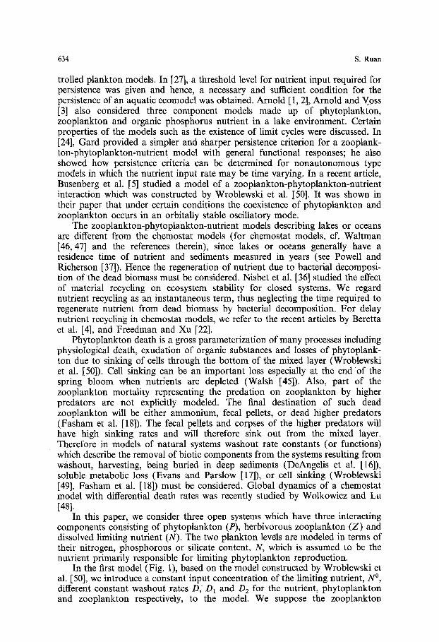
In the first model (Fig. 1), based on the model constructed by Wroblewski et al. [50], we introduce a constant input concentration of the limiting nutrient, N °, different constant washout rates D, ~ D1 and D2 for the nutrient, phytoplankton and zooplankton respectively, to the model. We suppose the zooplankton
Persistence and coexistence 635
[] , []
",,,\ //
NO (DN, D 1 P,D2Z)
Fig. 1. The Z - P - N model with constant nutrient input (N O ) and different washout rates (D, D 1 and D2). Arrows indicate nutrient flow pathways between phytoplankton (P), zooplankton (Z) and nutrient (N)
population feeds on both nutrient and phytoplankton (i.e., zooplankton is facultative or obligate), and only part of dead phytoplankton and zooplankton is recycled back into nutrients. We also use a general class of functions to describe nutrient uptake and functional response. Criteria for phytoplankton or zooplankton or both of them to become extinct, i.e., extinction thresholds, are derived. Boundedness of solutions is studied; this is essential for the model to be persistent. Existence of positive equilibria on both the N - P plane and the N - Z plane is considered which demonstrates that for the facultative predator model, the phytoplankton population can survive without zooplankton, and the zooplankton population too, can survive without phytoplankton. It is shown that subject to certain constraints, the system exhibits uniform persistence. In the case where the predator is obligate, we obtain criteria for persistence (and hence coexistence of both zooplankton and phytoplankton).
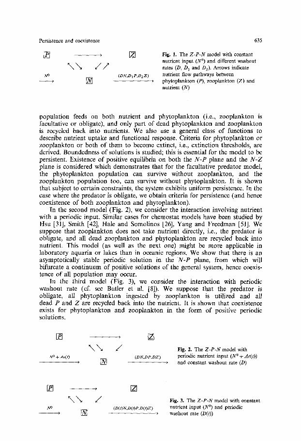
In the second model (Fig. 2), we consider the interaction involving nutrient with a periodic input. Similar cases for chemostat models have been studied by Hsu [31], Smith [42], Hale and Somolinos [26], Yang and Freedman [51]. We suppose that zooplankton does not take nutrient directly, i.e., the predator is obligate, and all dead zooplankton and phytoplankton are recycled back into nutrient. This model (as well as the next one) might be more applicable in laboratory aquaria or lakes than in oceanic regions. We show that there is an asymptotically stable periodic solution in the N - P plane, from which will bifurcate a continuum of positive solutions of the general system, hence coexis- tence of all population may occur.
In the third model (Fig. 3), we consider the interaction with periodic washout rate (cf. see Butler et al. [8]). We suppose that the predator is obligate, all phytoplankton ingested by zooplankton is utilized and all dead P and Z are recycled back into the nutrient. It is shown that coexistence exists for phytoplankton and zooplankton in the form of positive periodic solutions.
[] , []
\ \ / N O + Ae(t) (DN,DP,DZ)
, [ ]
Fig. 2. The Z - P - N model with periodic nutrient input (NO+ Ae(t))
and constant washout rate (D)
[]
\ \ NO
, [ ]
, [ ]
/ (D(t)N,D(t)P,D(t)Z)
Fig. 3. The Z - P - N model with constant nutrient input (N o ) and periodic washout rate (D(O)
636 S. Ruan
Persistence in biological systems in a context related to this paper has been discussed by many authors. We utilize the definitions of persistence developed by Butler et al. [7], and Butler and Waltman [9], namely if x(t) is such that x(t) > O, we say that x(t) persists if l im~fx ( t )>0 . Further, we say that x(t) persists
uniformly if there exists 6 > 0 such that lim inf x(t) >~ 6. Finally, a system persists (uniformly) if all components persist (uniformly).
2 Z - P - N model with constant nutrient input and washout rates
The instantaneous zooplankton-phytoplankton-nutrient (Z-P-N) model consist- ing of three interacting components, herbivorous zooplankton (Z), phytoplank- ton (P) and dissolved limiting nutrient (N), is given by the following set of ordinary differential equations
dN --~ = D(N ° - N) - aPu(N) - bZv(N) + (1 - ~)cZw(P) + ya P + 81Z
dP d--i = a e u ( N ) - c Z w ( P ) - (7 + D 1 ) P (2.1)
dZ - ~ = Z[bv(N) + 6cw(P) - (8 + D2)].
We assume that all parameters are non-negative and are interpreted as follows:
a -maximal nutrient uptake rate for the phytoplankton b -maximal nutrient uptake rate for the zooplankton c -maximal zooplankton ingestion rate N o -input concentration of the nutrient D -washout rate of the nutrient D1 -washout rate of the phytoplankton D2 -washout rate of the zooplankton 7 -phytoplankton mortality rate 8 -zooplankton death rate 71 -nutrient recycle rate after the death of the phytoplankton, 71 ~< 7 el -nutrient recycle rate after the death of the zooplankton, 81 ~< e 6 - the fraction of zooplankton nutrient conversion, 0 < 6 ~< 1.
Functions u(N) and v(N) describe the nutrient uptake rates of phytoplankton and zooplankton, respectively. We assume the following general hypotheses on the nutrient uptake functions (Hale and Somolinos [26]).
(i) The functions are non-negative, increasing and vanish when there is no nutrient.
(ii) There is a saturation effect when the nutrient is very abundant.
That is, we assume that u(N) and v(N) are continuous functions defined on [0, ~) , and satisfy
du u(0)=0 , ~ > 0 and u-,~lim u ( N ) = l , (2.2)
dv v(0)=0 , ~ > 0 and N-~oolim v (N)=I . (2.3)
Persistence and coexistence 637
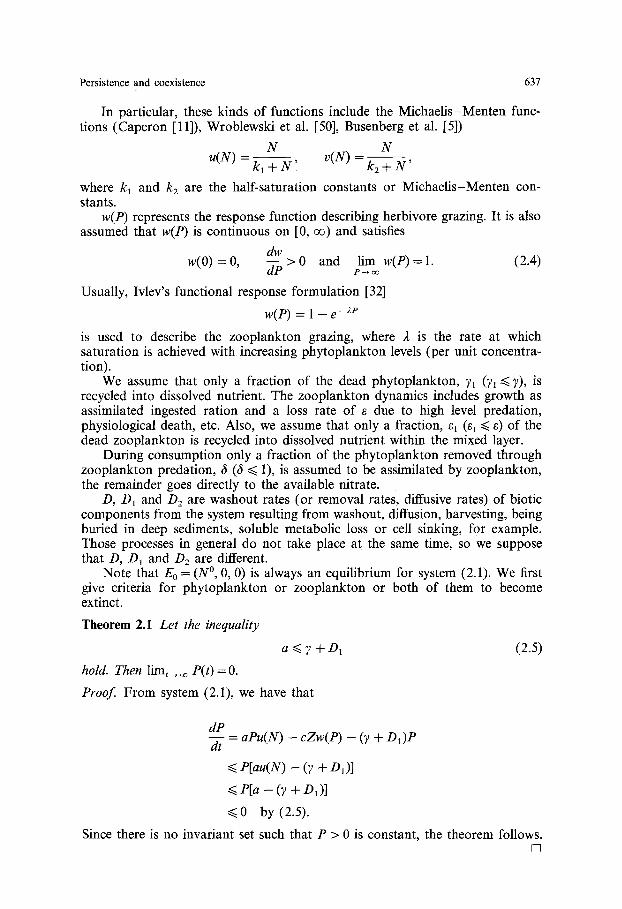
In particular, these kinds of functions include the Michaelis-Menten func- tions (Caperon [11]), Wroblewski et al. [50], Busenberg et al. [5])
N N u(N) - kl + ~ ', v(N) = k2 + N '
where kl and k2 are the half-saturation constants or Michaelis-Menten con- stants.
w(P) represents the response function describing herbivore grazing. It is also assumed that w(P) is continuous on [0, oo) and satisfies
dw w(0) = 0, ~-~ > 0 and e-~lim w(P) = 1. (2.4)
Usually, Ivlev's functional response formulation [32]
w(P) = 1 - e -~1,
is used to describe the zooplankton grazing, where 2 is the rate at which saturation is achieved with increasing phytoplankton levels (per unit concentra- tion).
We assume that only a fraction of the dead phytoplankton, 71 (71 ~< 7), is recycled into dissolved nutrient. The zooplankton dynamics includes growth as assimilated ingested ration and a loss rate of e due to high level predation, physiological death, etc. Also, we assume that only a fraction, gl (~1 ~ ~) of the dead zooplankton is recycled into dissolved nutrient within the mixed layer.
During consumption only a fraction of the phytoplankton removed through zooplankton predation, 6 (6 ~< 1), is assumed to be assimilated by zooplankton, the remainder goes directly to the available nitrate.
D, D1 and D2 are washout rates (or removal rates, diffusive rates) of biotic components from the system resulting from washout, diffusion, harvesting, being buried in deep sediments, soluble metabolic loss or cell sinking, for example. Those processes in general do not take place at the same time, so we suppose that D, D1 and D2 are different.
Note that E0 = (N °, 0, 0) is always an equilibrium for system (2.1). We first give criteria for phytoplankton or zooplankton or both of them to become extinct.
Theorem 2.1 Let the inequality
a ~< 7 + D1 (2.5)
hold. Then limt ~ 0o P(t) = O.
P r o o f From system (2.1), we have that
dP --~ = aPu(N) - cZw(P) - (~ + D1)P
<~ P[au(N) - (7 + D1)]
<<, P[a - (7 + D i)]
~<0 by (2.5).
Since there is no invariant set such that P > 0 is constant, the theorem follows.
638 S. Ruan
provided
Theorem 2.1 demonstrates that if the maximal nutrient uptake rate is less than or equal to the loss rate, then the phytoplankton population is eliminated.
Similarly, we can prove the following theorem.
Theorem 2.2 Let the inequality
b + 6c <<. ~ + D 2 (2.6)
hoM. Then lim Z(t) =0. t ~ o o
This result shows that the zooplankton population cannot exist if the summation of its maximal nutrient uptake rate and its net ingestion rate is less than or equal to its loss rate.
Corollary 2.3 I f (2.5) and (2.6) hold, then lim (N(t), P(t), Z(t)) =Eo. t---~ O0
By Corollary 2.3, if (2.5) and (2.6) hold, then both of the phytoplankton population and zooplankton population become extinct. In this case, it is not feasible for persistence of system (2.1).
If phytoplankton is the top trophic level, and zooplankton is set at zero, then we have the subsystem
dN dt - D(N° - N) - aPu(N) + 71P
(2.7) dP d t = P[au(U) - (7 + D1)].
System (2.7) has an interior equilibrium (N~, P~), where
el = 7 +D1-:7~
and
7 --I- D 1 < a (2.8)
u
So we have the following theorem.
Theorem 2.4 I f the inequalities (2.8) and (2.9) hold, then system (2.1) has a non-negative equilibrium E 1 = (NI , P 1 , 0 ) where N 1 and P1 are defined as above.
Similarly, we have
Theorem 2.5 I f the inequalities
and
+ D2 < b (2.10)
Persistence and coexistence 639
hold, then system (2.1) has a non-negative equilibrium E2 = (N2, O, Z2) where
Theorem 2.4 indicates that if (2.8) and (2.9) hold, then the phytoplankton population can survive on the nutrient, while Theorem 2.5 demonstrates that the predator zooplankton mag be able to survive on the nutrient without the prey phytoplankton if (2.10) and (2.11) hold. This is not true if (2.11) fails, and the equilibrium E2 does not exist.
Theorem 2.6 All solutions of system (2.1) are bounded.
Proof We have d dt (N + P + Z) = DN ° - DN + ?1P -b ~1 Z - - 7P -- D1P -- eZ -- D2Z
<~ -Do(N + P + Z) + DN °,
where D O = min{D, D1, O2}. The theorem follows. []
Theorem 2.7 I f the non-negative equilibria E1 and E2 exist, then (N 1, P1) and (N2, Z2) are globally asymptotically stable in the N-P plane and N-Z plane, respectively.
Proof We only prove the global asymptotic stability of (N1, P1) in the N-P plane; the stability of (N2, P2) in the N-Z plane can be proved similarly. Define a Liapunov function (cf. Harrison [30])
fN ru(x) -u(N1) au(N1)-~l f ~ X - P l dx. (2.12) V(N, P) = 1 u(~ dx -I- au(N1) ~
Then, if (2.8) holds, u(N~) - 71 > O, V(N, P) = 0 if and only i f N = N1, P = P1 and V(N, P) >>. 0 in the N-P plane. The time derivative of V along the trajectories of the subsystem (2.7) is
dV u(N) - u(Nl) [D(N 0 _ N) - aPu(N) + ?tP] dt u(N)
au(N1) - 71 + ~u(NO (P--P1)[au(U) --(7 +D1)]
F D ( N ° - N ) ( 7, ) = (u(N) -- u(N,)) L -~(2v) a -- u - ~ P
= (u(N) - u(N1) ) [ D(N°u(N)u(N~)- N1) + ~1P
= _ D(N ° -- Nx) + 7~P [u(N) - u(N1)] 2 - D u(N)u(NI ) u(N)
D(N - N, ) ] (u(g) - u(N~)) u(N) J
(N -- N~)(u(N) - u(N~ )).
640 s. Ruan
Since N1 < N °, the first term is negative. The second term is negative because u(N) is an increasing function. Thus, dV/dt <<, 0 and dV/dt = 0 if and only if N = N1. The largest invariant subset of the set of the point where dV/dt = 0 is (N1, P1). Therefore by LaSalle's theorem (LaSalle and Lefschetz [34]), (N1, P1) is globally asymptotically stable in the N-P plane. []
Theorem 2.8 I f the inequalities (2.8)-(2.11) hold and
by(N1) + 6cw(el) - (5 + D2) > 0 (2.13)
au(U2) - cZzw'(O) - (7 + D1) > 0, (2.14)
then system (2.1) is persistent.
Proof By Theorems 2.4 and 2.5, there are three equilibria on all the coordinate planes, i.e., E0 = (N °, 0, 0), El = (NI, P1,0) and E2 = (N2, 0, Z2). We first show that all equilibria are saddle points.
For Eo = (N °, 0, 0), the variational matrix of system (2.1) at Eo is
I i D - a u ( N ° ) + 7 1 -bV(oN°)+e I ] au(N°) - (7 + 91)
0 bv(N °) - (5 + O2)J
By inequalities (2.9) and (2.11), the eigenvalues of the variational matrix are 21 ~- - D < O, 2 2 = au(N °) - (7 + DI) > 0, 23 = bv(N °) - (5 + D2) > 0, SO E0 is a saddle point.
The variational matrix of system (2.1) at E1 = (N1, P~, 0) has the form
- O --aPlu'(N1) --au(N1) + Yl -by (N1) + ( 1 -6 ) cw(PO +51] aP1 u'(N1 ) 0 - cw(P1 ) ] ,
0 0 by(N1) + 6cw(P1) - (5 + D2) ]
and the eigenvalues of the variational matrix are 41,22 which are the roots of the equation
2 2 + (D + aPlu'(Nl))4 + aPlu'(N1)(au(Nl) - 71) = 0
and
23 = by(N1) + 6cw(P1) - (5 + D2).
Clearly, 41 and 42 have negative real parts, and )~3 > 0 by condition (2.13). Therefore E1 is a saddle point, and since 4 3 > 0, El is unstable in the direction orthogonal to the N-P coordinate plane.
The variational matrix of system (2.1) at E2 = (N2, 0, Z2) has the form
I - D - b Z : v ' ( N 2 ) - a u ( N z ) + ( 1 - f ) e Z 2 w ' ( O ) + Y a - b y ( N 2 ) + 5 1 ] au(N2) - (7 + D1) - eZ2w'(O) 0 .
~. - bZ2v (N2) 6cg2w'(O) 0
By analogous arguments to those analyzing E1 and condition (2.14), we can prove that E2 is a saddle point, and it is unstable in the direction orthogonal to the N - Z coordinate plane.
Now let
cZw(P) G(N, P, Z) = au(N) p (7 + D,),
H(N, P, Z) = by(N) + 6cw(P) - (5 + D2).
Persistence and coexistence 641
We have that
H(N1, P1, O) = by(N1) + 6cw(P1) - (5 + D2) > 0
G(N2, 0, Z2) = au(N2) - cZ2w'(O) - (~ + Da) > O.
According to Theorem 5.1 of Freedman and Waltman [20], system (2.1) is persistent. This completes the proof. []
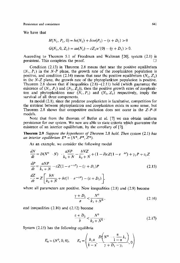
Condition (2.13) in Theorem 2.8 means that near the positive equilibrium (Na, P1) in the N-P plane, the growth rate of the zooplankton population is positive, and condition (2.14) means that near the positive equilibrium (N2, Z2) in the N-Z plane, the growth rate of the phytoplankton population is positive. Theorem 2.8 shows that if inequalities (2.8)-(2.11) hold (which guarantee the existence of (NI, Pa) and (N2, Z2)), then the positive growth rates of zooplank- ton and phytoplankton near (N~, P~) and (N2, Z2) respectively, imply the survival of all three components.
In model (2.1), since the predator zooplankton is facultative, competition for the nutrient between phytoplankton and zooplankton exists in some sense, but Theorem 2.8 shows that competitive exclusion does not occur in the Z-P-N models.
Note that from the theorem of Butler et al. [7] we can obtain uniform persistence for our system. We now are able to state criteria which guarantee the existence of an interior equilibrium, by the corollary of [7].
Theorem 2.9 Suppose the hypotheses of Theorem 2.8 hoM. Then system (2.1) has an interior equilibrium E* = (N*, P*, Z*).
As an example, we consider the following model
dN aNP bNZ - ~ = D ( N ° - N ) k l + N k 2 + N + ( 1 - ~ ) c Z ( 1 - e - ' t e ) + 7 1 P + ~ 1 Z
dP aNP c Z ( 1 - e ze) _(~ + D,)P (2.15)
dt " k~ + N
dZ Z ~ bN + -~e) ] = c(l--e - ( 5 + D 2 ) ,
where all parameters are positive. Now inequalities (2.8) and (2.9) become
7 + D1 N O --. NO, (2.16) a kl +
and inequalities (2.10) and (2.12) become
e + D 2 N O < k2 + N ~ " (2.17)
System (2.15) has the following equilibria
1 - ~ , 0 " / \ 1 - ~ ' 7+D~ ~1
642 s. Ruan
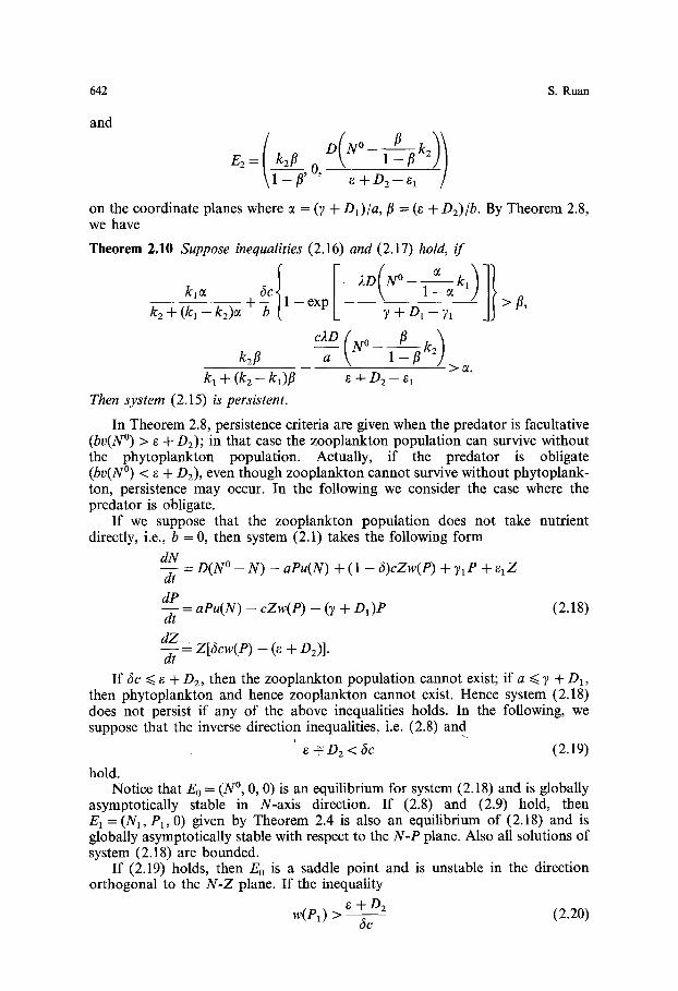
and
E2= ,0, ~ + D2 El
on the coordinate planes where ~ = (7 + D~)/a, fl = (~ + D2)/b. By Theorem 2.8, we have
Theorem 2.10 Suppose inequalities (2.16) and (2.17) hoM, if
kj
k 2 + ( k l - k 2 ) ~
k2/ ka + (kz - kl)fl
Then system (2.15) is persistent.
- e x p -7~ D( - - -~
c2D ( N ° fl k2)
a 1 - f l >or.
In Theorem 2.8, persistence criteria are given when the predator is facultative (bv(N °) > e + D2); in that case the zooplankton population can survive without the phytoplankton population. Actually, if the predator is obligate (bv(N °) < e + D2), even though zooplankton cannot survive without phytoplank- ton, persistence may occur. In the following we consider the case where the predator is obligate.
If we suppose that the zooplankton population does not take nutrient directly, i.e., b = 0, then system (2.1) takes the following form
dN --~ = D(N ° - N) - aPu(N) + (1 - 6)cZw(P) + 71P + I~lZ
dP - ~ = aPu(N) - cZw(P) - (7 + D,)P (2.18)
dZ d-T = Z[6cw(P) - (~ + D2) ].
If 6c <<. e + D2, then the zooplankton population cannot exist; if a ~< 7 + D1, then phytoplankton and hence zooplankton cannot exist. Hence system (2.18) does not persist if any of the above inequalities holds. In the following, we suppose that the inverse direction inequalities, i.e. (2.8) and
-F D2 < 6c (2.19)
hold. Notice that E0 = (N °, 0, 0) is an equilibrium for system (2.18) and is globally
asymptotically stable in N-axis direction. If (2.8) and (2.9) hold, then E1 = (N1, P~, 0) given by Theorem 2.4 is also an equilibrium of (2.18) and is globally asymptotically stable with respect to the N-P plane. Also all solutions of system (2.18) are bounded.
If (2.19) holds, then E0 is a saddle point and is unstable in the direction orthogonal to the N - Z plane. If the inequality
+ D 2 w(PO > - (2.20)
de
Persistence and coexistence 643
holds, then E 1 is a saddle point and is unstable in the direction orthogonal to the N-P plane. Hence by Butler-McGehee lemma (cf. [21]), inequality (2.20) implies the persistence of system (2.18). It is known that persistence of the Z component is equivalent to entire system persistence (Gard and Hallam [25]) for models of the form (2.18). Following the similar arguments by Hallam [27, 28] and Gard [24], we know that condition (2.20) is also necessary for persistence in system (2.18). The result in [7] implies that system (2.18) processes an interior equi- librium E* = (N*, P*, Z*) with
p , = w_l (e "l- D2 "] \ ~ - c f " (2.21)
Theorem 2.11 Assume (2.8), (2.9) and (2.19) hold. Then system (2.18) persists i f and only i f (2.20) holds. Furthermore, under (2.20) system (2.18) has a positive interior equilibrium.
This result indicates that solutions of system (2.18) are uniformly ultimately bounded and have components which do not tend to zero under certain conditions. Condition (2.20) means that near the positive equilibrium (N1, P1) in the N-P plane, the growth rate of zooplankton is positive.
Notice also that the right hand side of inequality (2.20) is the value of the function w(P) at P* by (2.21). So condition (2.20) is equivalent to w(P1) > w(P*). Since w(P) is increasing by (2.4), it is also equivalent to P1 > P*.
Now we consider (2.15) with b = 0, kl = k, namely
dN aNP --~ = D ( N ° - N ) - k +----N + (1 - 6 ) c Z ( 1 - e - ' t e ) + 7 1 P + •1 z
dP aNP cZ(1 - e-he) _ (7 + D1)P (2.22)
dt - k + N dZ --~ = Z[6c( 1 - e -he) _ (e + D2)].
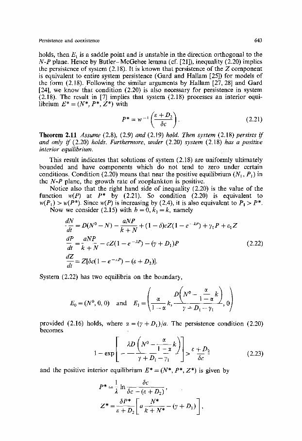
System (2.22) has two equilibria on the boundary,
E o = ( N O ,0,0) and E1 = ~ k, 1 - e ,0 7 +D1 -71
provided (2.16) holds, where ~ = (7 +D1)/a. The persistence condition (2.20) becomes
1 e x p 1 - ~ e + D 2 - > - - (2.23) 7 + D1 - 71 66'
and the positive interior equilibrium E* = (N*, P*, Z*) is given by
1 6e P* = ~ In 6e - (e + D2) '
6P* ~ N* -] z * = + D=Lak---+--~-(7 + D1)J ,
644 s. Ruan
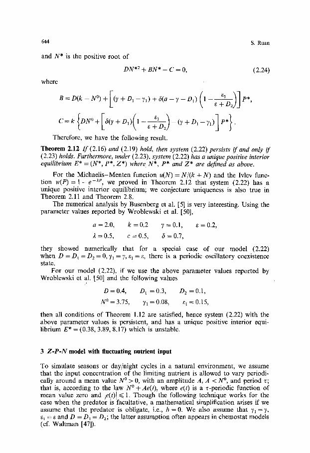
and N* is the positive root of
where
DN .2 + BN* - C = O, (2.24)
. o1, (, )J. .
Therefore, we have the following result.
Theorem 2.12 I f (2.16) and (2.19) hold, then system (2.22)persists if and only if (2.23) holds. Furthermore, under (2.23), system (2.22) has a unique positive interior equilibrium E* = (N*, P*, Z*) where N*, P* and Z* are defined as above.
For the Michaelis-Menten function u(N) = N/(k + N) and the Ivlev func- tion w(P)= 1 - e -ae, we proved in Theorem 2.12 that system (2.22) has a unique positive interior equilibrium; we conjecture uniqueness is also true in Theorem 2.11 and Theorem 2.8.
The numerical analysis by Busenberg et al. [5] is very interesting. Using the parameter values reported by Wroblewski et al. [50],
a = 2 . 0 , k = 0 . 2 7 = 0 . 1 , e = 0 . 2 ,
2 = 0 . 5 , c = 0 . 5 , 6 = 0 . 7 ,
they showed numerically that for a special case of our model (2.22) when D = D I = D 2 = 0, 71 = 7, el = e, there is a periodic oscillatory coexistence state.
For our model (2.22), if we use the above parameter values reported by Wroblewski et al. [50] and the following values
/ i
D = 0.4, D1 = 0.3, D2 --- 0.1,
N O = 3.75, 71 : 0.08, el : 0.15,
then all conditions of Theorem 1.12 are satisfied, hence system (2.22) with the above parameter values is persistent, and has a unique positive interior equi- librium E* = (0.38, 3.89, 8.17) which is unstable.
3 Z - P - N model With fluctuating nutrient input
To simulate seasons or day/night cycles in a natural environment, we assume that the input concentration of the limiting nutrient is allowed to vary periodi- cally around a mean value N O > 0, with an amplitude A, A < N °, and period v; that is, according to the law N ° + Ae(t), where e(t) is a v-periodic function of mean value zero and le(t)] ~< 1. Though the following technique works for the case when the predator is facultative, a mathematical simplification arises if we assume that the predator is obligate, i.e., b = 0. We also assume that 71---7, el = e and D = D 1 = D 2 ; the latter assumption often appears in chemostat models (cf. Waltman [47]).
Persistence and coexistence 645
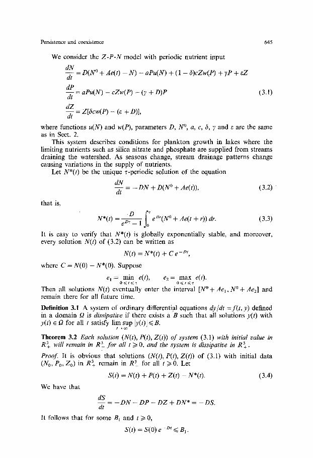
We consider the Z - P - N model with periodic nutrient input
dN d----[ = D(N° + Ae(t) - N) - aPu(N) + ( 1 - 6)cZw(P) + vP + eZ
~ = aPu(U) - cZw(P) - (~ + D)P (3.1)
dZ = Z[rcw(P) - (e + D)],
where functions u(N) and w(P), parameters D, N °, a, c, 3, 7 and e are the same as in Sect. 2.
This system describes conditions for plankton growth in lakes where the limiting nutrients such as silica nitrate and phosphate are supplied from streams draining the watershed. As seasons change, stream drainage patterns change causing variations in the supply of nutrients.
Let N*(t) be the unique ~-periodic solution of the equation
dN - - = - D N ÷ D(N ° + Ae(t)), (3.2) dt
that is,
N*(t) - D eDr(N ° + Ae(t + r)) dr. (3.3) e D¢- 1
It is easy to verify that N*(t) is globally exponentially stable, and moreover, every solution N(t) of (3.2) can be written as
N(t) = N*(t) + C e-Dr,
where C = N(0) - N*(0). Suppose
el = rnin e(t), e2 = max e(t). O<~t<~z O<~t<~
Then all solutions N(t) eventually enter the interval [N°+ Ael, N ° + Ae2] and remain there for all future time.
Definition 3.1 A system of ordinary differentiM equations dy/dt =f ( t , y) defined in a domain O is dissipative if there exists a B such that all solutions y(t) with y(t) ~ f2 for all t satisfy lim sup [y(t)] ~< B.
Theorem 3.2 Each solution (N(t), P(t), Z(t)) of system (3.1) with initial value in R3+ will remain in R3+ for all t >>. O, and the system is dissipative in R3+.
Proof. It is obvious that solutions (N(t), P(t), Z(t)) of (3.1) with initial data (No, Po, Zo) in R~_ remain in R3+ for all t ~> 0. Let
S(t) = N(t) + P(t) + Z(t) - N*(t). (3.4)
We have that
dS - D N - D P - D Z + D N * = - D S .
dt
It follows that for some B 1 and t ~> 0,
S(t) = S(O) e-Dr < B1"
646 s. Ruan
Thus, for t ~> 0
U(t) + P(t) + Z(t) <<. N*(t) + B1.
Since N*(t) is a globally exponentially stable periodic solution of (3.2), there is a B such that
lim sup [N(t) +P( t ) + Z(t)] < B, (3.5) t ---~ o o
that is, system (3.2) is dissipative in R 3. []
We know that in an Euclidean space g, a periodic ordinary differential equation is equivalent to a dynamical system re(x, t) on a cylinder E = g × with a flow ~-, where ~ = [0, z]/{0, z} is a quotient space of [0, 3] by identifying 0 and z, or ~ can be regarded as a nontrivial circle on the plane. We think of E as a subset of 8 x R 2. In fact, for system (3.1), g = R × R3+. To study the asymptotic behavior of solutions of (3.1), we only need to study the t2-fimit sets of trajectories of a dynamical system n with flow ~ on E.
For each point x e E, we denote it by x = (N, P, Z, Q), where Q e 2. Let 0Ee = {(N, P, Z, Q) e E [ P = 0}, aEz = {(N, P, Z, Q) e E I z = 0}. We denote the restrictions of flow ~ to OEe and OEz by O~e and d ~ z , respectively. A + (x) denotes the omega limit of the orbit through x.
Definition 3.3 An isolated invariant set M for the flow .~ is a nonempty invariant set which is the maximal invariant set in some neighbourhood of itself. Note that if M is a compact, isolated invariant set, one may always choose a compact isolating neighbourhood.
For an isolated invariant set M c E, we define
W +(M) = {x e E [ A+(x) n M ~ ~ }
as the weak stable set and
W + ( M ) = {x e E IA+(x) v~ ~ and A +(x) c M}
as the stable set, and we denote
~ ( M ) = U A+(x) • x E M
Define M = {(N*(t), 0, 0, Q) e E I Q e ~}, then M is a compact invariant set for ~ . It is easy to verify that the boundaries ~Ee, ~Ez and hence ~E = aEe LJ aEz are invariant. Moreover, we have
Lemma 3 . 4 0 E e c W + ( M ) such that if x e ~E?\M, then
Ll (x, t)II °0 a s t - , -
Proof. Since Z(t) = Z(0) e-(,+D)t whenever x = (No, 0, Zo, 0) e OE~, we have re(x, t) = (N(t), O, Z(t), t mod(z)) -o (N*(Q(t)), O, O, Q(t)) as t ~ oo, Q e [0, z], i.e., OEe c W+(E). On the other hand, for x e dEe\M, since N(t) = N*(t) + C e -Dr for some constant C 4 0 whenever N ( t o ) # N * ( t o ) for any to e [0, z], then N(t) # U*(t). Therefore II (x, t)I[ ~ oo as t-~ -- ~ . []
Let B(z) denote the Banach space of continuous z-periodic real valued functions x : R -~ R under the supremum norm
Ixl0= sup Ix(t)]. O <~ t <~ "r
Persistence and coexistence 647
Let B+ (z) = {x • B(O Ix(t) > 0 for all t} and
1 x(t) dt. (x(t) ) z
The following result indicates that if the phytoplankton population has positive growth rate near the stable periodic solution N*(t) of (3.2), then it is persistent.
Theorem 3.5 I f
~o = a(u(N*(t))) - (7 + D) > 0, (3.6) \
then
lira inf P( t) > O. t ~ O O
Proof First we prove that M is isolated. Since ao > 0 and u(N) is continuous, there is Ao > 0 such that for some ~ > 0
a(u(N*(t + ~) - Ao) ) - (7 + D + Ao)/> ? > 0. (3.7)
Since o~ is dissipative, we can find ~ > 0 and to ~> 0 such that 0 ~< P(t) <<. ~ for all t ~> to. Define
Ao L = c max w(P)>O and A = - L >0"
0 <~ P(t) <~
Then .Ar~ = {x ~ EIQ(x, M) < A } is an isolating neighbourhood of M, where ~ is the metric of E. Otherwise, there is an invariant set G containing M in JV'~ with G \ M ¢ ~ . Lemma 3.3 implies that ( G \ M ) n O E e = ~ . Therefore for any x • G \M, then x ¢ OEp, i.e., P0 > 0. Since G is invariant, ~+(x) c G c ~/'~ where 7 +(x) is the positive semiorbit through x. Now we have
d [ln P(t)] ~> au(N*(t) - Ao) - (7 + O + Ao) in Jlr a .
From (3.7) it follows that
P(nz)>~Poexp ~ n z ~ o e asn--*o%
a contradiction to ~(x, nz) e G for all n ~> O. So M is isolated. Now for any x • E and re(x, t) = (Nx(t), Px(t), Zx(t), t mod(~)), if lira inf
t ~ o o
Px(t)=O, then A + ( x ) n O E e C f g , - a n d hence M c A + ( x ) , s o Ww+(M)= {x • E l l iminfP~( t ) =0}. We claim that for any x • E\~Ee, if A +(x) e M, then
there exists e > 0 such that
IN~(t) - N * ( t + a ) l ~ 0 as t ~ o o .
In fact, if A +(x) = M, then Px(t) and Zx(t) tend to zero as t ~ o% which implies Nx(t) - N*(t + ~) tends to zero for some c~ > 0. Hence
lim [a (u (N( t ) ) ) - (7 + D)] = a 0 > 0 l ~ o O
and l iminfP~(t) >0, a contradiction to A +(x) ~OEp # ~ , i.e., x ¢ W+(M), by
Lemma 3.4 we have W+(M) = OEe, so x • W + ( M ) \ W + ( M ) . Hence by Theo- rem 4.1 of Butler and Waltman [9], A +(x) n ( W + ( M ) \ M ) # (g. It follows from
648 S. Ruan
Lemma 3.4 that A +(x) is unbounded, a contradiction to the dissipativeness of f t . Hence A +(x)~OEe = ~ , and A÷(x ) is compact, so Q(A +(x), OEe)> O, i.e., lim inf P( t) > O. []
t - - ~
Theorem 3.6 I f o- o > 0, then there ex&ts a nontrivial asymptotically stable z-peri- odic orbit on OEz.
Proof Define a Poincar6 map T from P - Z plane to itself by T(No, Po) = (N(z), P(z)). By Theorem 3.5 and the dissipativity for each (No, Po) in the interior of R2+, {Tn(N0, Po)} has a convergent subsequence. So by Massera's fixed point theorem (see Sansone and Conti [41]), there exists a fixed point (N, P) of T in the interior of R2+, which gives a nontrivial periodic orbit on OEz.
We observe that v(N, P, t) -- N + P is a solution of the initial-boundary value problem
I v, + [D(N ° + Ae(t) - N) - (au(N) - 7)P]vN
+ [(au(N) -- (~ + D)P]u e + Du = D(N ° + Ae(t))
v(N, 0, t) = N*(t), v(N, P, O) = v(N, P, z), t ~ [0, z], N/> 0, P >~ 0.
By Theorems 3.7 and 3.8 of Yang and Freedman [51], the nontrivial z-periodic orbit on ~Ez is asymptotically stable. This completes the proof. []
Let (N, P) be the asymptotically stable z-periodic solution of the reduced system
dN dt - D(N° + Ae(t) - N) - aPu(N) + 7P
aP (3.8) d-t = P[au(N) - (y + D)]
in Theorem 3.6. We will show in the following that this solution of (3.8) yields a solution (N, P, Z) = (N, P, 0) ~ B3+ (z) of system (3.1) from which will bifur- cate a continuum of positive solutions of (3.1) using ~ as the bifurcating parameter.
To do this by means of Theorem 1 of Cushing [14], it is necessary that the solution (N, P) of the reduced system (3.8) be noncritical; i.e., that the linearized system of (3.8) at (N, P) have no Floquet exponents with zero real part. We assume throughout that (N, P) is stably noncritical, i.e., that these Floquet exponents have negative real parts.
Theorem 3.7 Assume ao > 0 and that (N, P ) E B 2 (z) is a stably noncritical solution of (3.8). Then there exists a set 11+ = {(N, P, Z, #) ~ B3+ (z) x R} with (N_, P , Z ) > 0 solving (3.1), the closure of 1I + is a continuum which connects (N, P~ 0,/~) 6 B3(z) x R,/~ = - (cw@)) , to a solution of the form (N, P, 0,/~) ~ B3(z) × R, where (N, P, O, ~t) v~ (N, P, O, ~t), N > 0 and P > O.
Proof Define 123 = {(N, P, Z) e R 3 I N > 0}, by Theorem 1 of Cushing [14] with d2(t) = - # = - ( e + D ) , there is a continuum C+ c B 3 ( z ) x R of solutions of (3.1) which contains the bifurcating point (N, P, 0, fi) and which connects to the boundary of the set O 3 x R c B 3 ( z ) x R, where f2~ = {(N, P , Z ) B3(~) I N + N > 0}. And in an open neighborhood of (N, P, 0, fi), the set C+/ {(N, P, 0,/~)} consists of positive solutions of (3.1). The continuum C ÷ cannot
Persistence and coexistence 649
consist entirely of positive solutions, otherwise, in order to connect to the boundary of 0 3 × R, C + would have to be unbounded which would contradict Theorem 3.2. Thus C + must leave the positive cone B 3 (r) × R at a point other than the bifurcating point.
Denote by C + the maximal subcontinuum of C + which connects (N, P, 0, fi) to the boundary of B 3 (z) x R and define H + = C + ~ (B3+ (z) × R). Then the closure of H + is a continuum which connects (N, P, 0, ~) to the boundary of B3+(v) × R, i.e., the closure of H + contains (N,P,O,~t ) and a point (N, P, 0, fi) # (N, P, 0, fi) where N ~> 0 and /3 ~> 0.
~ Let (Nn, Pn, O, ktn)~H + b e a sequence which converges in B3('C)xR to (N, P, 0,/~). If (N, P, Z ) = (N, P, 0), dividing the second equation of (3.1) by P, > 0 and taking average, we obtain
( a u ( N , ) ) = 7 + D. (3i9)
If _N = 0, let n ~ o0 in (3.9), then we get a contradiction to 7 + D > 0. Hence it must be the case N > 0.
I f /~ - 0, then from the first equation of (3.1) in the limit as n --* 0% we see that N e B+ (z) solves the periodic equation (3.2) and hence N = N*. From (3.9), i t follows that ( a u ( N * ) ) = 7 + D, a contradiction to a0 > 0. Hence N > 0 and P > 0 . []
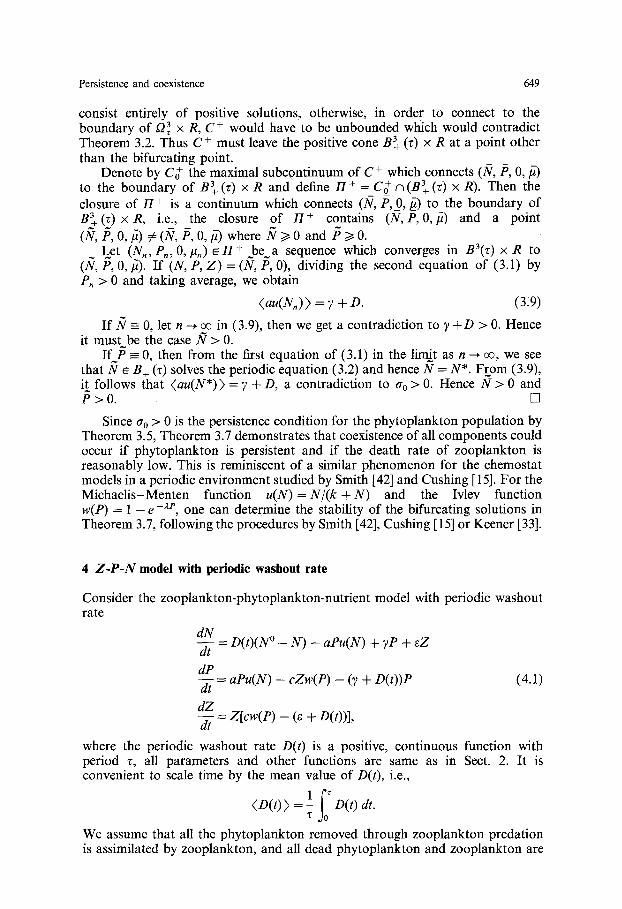
Since % > 0 is the persistence condition for the phytoplankton population by Theorem 3.5, Theorem 3.7 demonstrates that coexistence of all components could occur if phytoplankton is persistent and if the death rate of zooplankton is reasonably low. This is reminiscent of a similar phenomenon for the chemostat models in a periodic environment studied by Smith [42] and Cushing [ 15]. For the Michaelis-Menten function u(N) = N / ( k + N ) and the Ivlev function w(P) = 1 - e -he, one can determine the stability of the bifurcating solutions in Theorem 3.7, following the procedures by Smith [42], Cushing [ 15] or Keener [33].
4 Z-P-N model with periodic washout rate
Consider the zooplankton-phytoplankton-nutrient model with periodic washout rate
d N d--t = D( t ) (N° - N ) - aPu(N) + yP + eZ
dP d t = aPu(N) - cZw(P) - (~ + O(t ) )P (4.1)
d Z - ~ = Z [ c w ( e ) - (~ + D(t))],
where the periodic washout rate D(t) is a positive, continuous function with period r, all parameters and other functions are same as in Sect. 2. It is convenient to scale time by the mean value of D(t), i.e.,
;o 1 D(t) at. ( D ( t ) ) = z
We assume that all the phytoplankton removed through zooplankton predation is assimilated by zooplankton, and all dead phytoplankton and zooplankton are
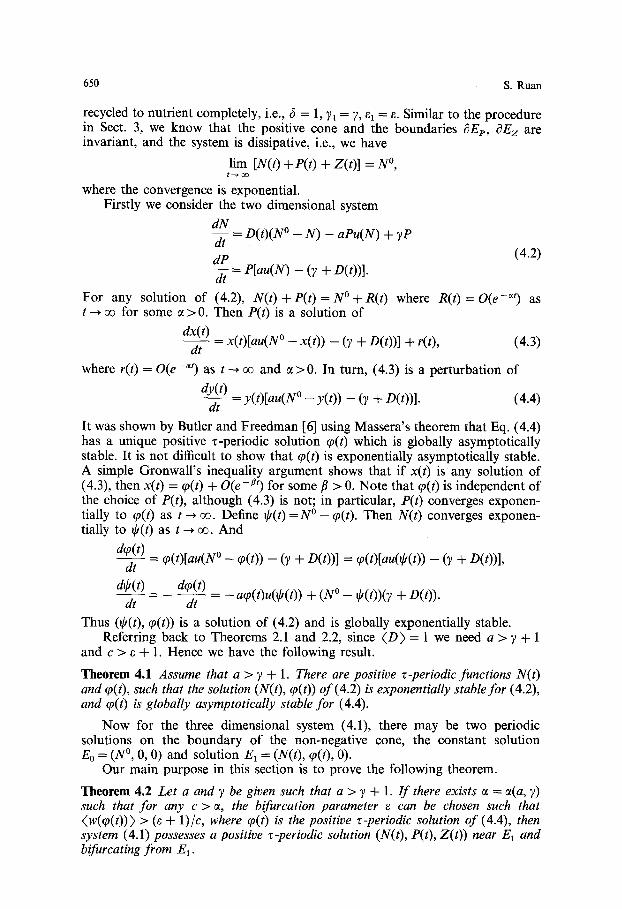
650 S. Ruan
recycled to nutrient completely, i.e., 6 = 1, 71 = 7, e, --- e- Similar to the procedure in Sect. 3, we know that the positive cone and the boundaries dEe, ~Ez are invariant, and the system is dissipative, i.e., we have
lim [N(t) + P(t) + z ( t ) ] = N °, t --~ OO
where the convergence is exponential. Firstly we consider the two dimensional system
dN dt - D(t)(N° - N) - aPu(N) + 7P
dP (4.2) -d~ = P[au(U) - (7 + D(t))].
For any solution of (4.2), N ( t ) + P ( t ) = N ° + R(t) where R ( t ) = O(e -~t) as t ~ ~ for some ~ > 0. Then P(t) is a solution of
dx(t) = x(t)[au(NO _ x(t)) - (7 + D(t))] + r(t), (4.3) dt
where r(t) = O(e - ' t ) as t ~ ~ and ~ >0. In turn, (4.3) is a perturbation of
dy(t) _ y(t)[au(N o _ y(t)) - (? + D(t))]. (4.4) dt
It was shown by Butler and Freedman [6] using Massera's theorem that Eq. (4.4) has a unique positive z-periodic solution ~0(t) which is globally asymptotically stable. It is not difficult to show that ~p(t) is exponentially asymptotically stable. A simple Gronwall's inequality argument shows that if x(t) is any solution of (4.3), then x(t) = q)(t) + O(e-#t) for some fl > 0. Note that (p(t) is independent of the choice of P(t), although (4.3) is not; in particular, P(t) converges exponen- tially to q~(t) as t--* oe. Define O( t )=N O- q~(t). Then N(t) converges exponen- tially to O(t) as t ~ oo. And
do(t) _ q)(t)[au(N o _ q)(t)) - (7 + D(t))] = q)(t)[au(#/(t)) - (? + D(t))], dt
dry(t) dq~( t) dt - dt - aqg(t)u(~k(t)) + (N O - ~b(t))(? 4- D(t)).
Thus (~(t), ~o(t)) is a solution of (4.2) and is globally exponentially stable. Referring back to Theorems 2.1 and 2.2, since <D) = 1 we need a > ? + 1
and c > e + 1. Hence we have the following result.
Theorem 4.1 Assume that a > 7 + 1. There are positive z-periodic functions N(t) and q~(t), such that the solution (N(t), q~(t)) of (4.2) is exponentially stable for (4.2), and ¢p(t) is globally asymptotically stable for (4.4).
Now for the three dimensional system (4.1), there may be two periodic solutions on the boundary of the non-negative cone, the constant solution Eo = (N °, 0, 0) and solution E1 = (N(t), q~(t), 0).
Our main purpose in this section is to prove the following theorem.
Theorem 4.2 Let a and ? be given such that a > ? + 1. I f there exists ~ = ct(a, 7) such that for any c > ~, the bifurcation parameter e can be chosen such that <w(q~(t)) > > (e + 1)/c, where ¢p(t) is the positive z-periodic solution o f (4.4), then system (4.1) possesses a positive z-periodic solution (N(t), P(t), Z(t)) near E1 and bifurcating f rom El .
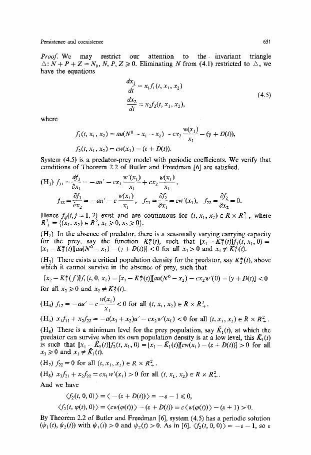
Persistence and coexistence 651
P r o o f We may restrict our a t tent ion to the . invariant triangle A: N + P + Z = No, N, P, Z ~> 0. Eliminating N f rom (4.1) restricted to A, we have the equat ions
dxl = X l f l ( t , Xl, X2)
dt dx2 (4.5) dt = xzf2(t, Xa, x2),
where
f l ( t , Xl, x2) = au(N ° - - x 1 - x2) -- c x 2 W(Xl) - (7 "[- D(t)), Xl
f2(t , Xl, x2) = cw(xl ) -- (~ + D(t)).
System (4.5) is a predator-prey model with periodic coefficients. We verify that condit ions o f Theorem 2.2 o f Butler and Freedman [6] are satisfied.
dfl w'(xa) W(Xl) (H1) f l l - - au' - cx2 + c x 2 - - ,
~ x l x I X1
f12 Of 1 W(X,) ~f2 Ofz - O x ~ 2 - a u ' - c , f 2 , - = c w ' ( x , ) , f 22= - = 0 .
X 1 OX 1 OX 2
Hence f j ( i , j = 1, 2) exist and are cont inuous for (t, Xl, x 2 ) ~ R x R2+, where = {(x, , R 2, x, i> 0, x2/> 0}.
(H2) In the absence of predator , there is a seasonally varying carrying capacity for the prey, say the funct ion K*(t) , such that [ X l - K*(t)] f l ( t , Xl, O ) = [xl - K*(t)][au(N ° - Xl) - (7 + D(t))] < 0 for all Xl > 0 and Xl ~ K*(t) .
(H3) T h e r e exists a critical popula t ion density for the predator , say K*(t) , above which it cannot survive in the absence of prey, such that
Ix2 - K * ( f ) ] f l ( t , 0, x2) = [x2 - K*(t)][au(N ° - x2) - cx2w'(O) - (7 + D(t)] < 0
for all x2 ~> 0 and x2 ~ K* (t).
W(X1) (H4) f12 = - - a t / ' - C < 0 for all (t, x l , x2) ~ R × R2+.
X1
(Hs) xtf11 + xzf22 = - a ( x l + x2)u' - cx2w' (x l ) < 0 for all (t, x l , x2) ~ R × R 2 .
(H6) There is a minimum level for the prey populat ion, say/£1 (t), at which the preda tor can survive when its own popula t ion density is at a low level, this/~1 (t) is such that [Xl -2 R~(t)]f2(t, x~, 0) = [Xl - Rl(t)][cw(x~) - (~ + D(t))] > 0 for all Xl >t 0 and Xl # KI(0 .
(H7) f22 = 0 for all (t, Xl, x2) ~ R × R2+.
(Hs) Xlf21 "~ x2f22 = C X l W * ( X l ) > 0 for all (t, Xx,X2) ~ R x R2+.
And we have
(f2 (t, O, O) ) = ( - (e + D(t ) ) ) = -- e - 1 ~< O,
(f2(t, g0(t), 0 ) ) = (cw(go(t)) ) -- (e + D(t)) = c(w(go(t)) ) -- (g + 1) > 0 .
By Theorem 2.2 o f Butler and Freedman [6], system (4.5) has a periodic solution (¢~(t), ¢2(t)) with ¢1(0 > 0 and ¢2(t) > 0 . As in [6], (f2(t, 0, 0 ) ) = - ~ - 1, so
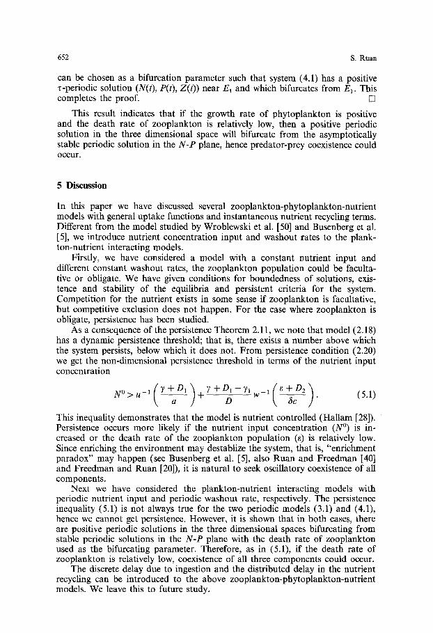
652 S. Ruan
can be chosen as a bifurcation parameter such that system (4.1) has a positive z-periodic solution (N(t), P(t), Z(t)) near E1 and which bifurcates from E 1 . This completes the proof. []
This result indicates that if the growth rate of phytoplankton is positive and the death rate of zooplankton is relatively low, then a positive periodic solution in the three dimensional space will bifurcate from the asymptotically stable periodic solution in the N-P plane, hence predator-prey coexistence could o c c u r .
5 Discussion
In this paper we have discussed several zooplankton-phytoplankton-nutrient models with general uptake functions and instantaneous nutrient recycling terms. Different from the model studied by Wroblewski et al. [50] and Busenberg et al. [5], we introduce nutrient concentration input and washout rates to the plank- ton-nutrient interacting models.
Firstly, we have considered a model with a constant nutrient input and different constant washout rates, the zooplankton population could be faculta- five or obligate. We have given conditions for boundedness of solutions, exis- tence and stability of the equilibria and persistent criteria for the system. Competition for the nutrient exists in some sense if zooplankton is facultative, but competitive exclusion does not happen. For the case where zooplankton is obligate, persistence has been studied.
As a consequence of the persistence Theorem 2.11, we note that model (2.18) has a dynamic persistence threshold; that is, there exists a number above which the system persists, below which it does not. From persistence condition (2.20) we get the non-dimensional persistence threshold in terms of the nutrient input concentration
+ w . ( 5 . 1 ) a D 6c
This inequality demonstrates that the model is nutrient controlled (Hallam [28]). Persistence occurs more likely if the nutrient input concentration (N °) is in- creased or the death rate of the zooplankton population (~) is relatively low. Since enriching the environment may destablize the system, that is, "enrichment paradox" may happen (see Busenberg et al. [5], also Ruan and Freedman [40] and Freedman and Ruan [20]), it is natural to seek oscillatory coexistence of all components.
Next we have considered the plankton-nutrient interacting models with periodic nutrient input and periodic washout rate, respectively. The persistence inequality (5.1) is not always true for the two periodic models (3.1) and (4.1), hence we cannot get persistence. However, it is shown that in both cases, there are positive periodic solutions in the three dimensional spaces bifurcating from stable periodic solutions in the N-P plane with the death rate of zooplankton used as the bifurcating parameter. Therefore, as in (5.1), if the death rate of zooplankton is relatively low, coexistence of all three components could occur.
The discrete delay due to ingestion and the distributed delay in the nutrient recycling can be introduced to the above zooplankton-phytoplankton-nutrient models. We leave this to future study.
Persistence and coexistence 653
Acknowledgements. The author would like to thank the two referees for their invaluable comments and helpful suggestions that greatly improved the original version of the paper; he is also grateful to Dr. S. Busenberg for a stimulating talk on this paper.
References
1. Arnold, E. M.: Aspects of a zooplankton, phytoplankton and phosphorus system. Ecol. Model. 5, 293-300 (1978)
2. Arnold, E. M.: On stability and periodicity in phosphorus nutrient dynamics. Q. Appl. Math. 38, 139 141 (1980)
3. Arnold, E. M., Voss, D. A.: Numerical behavior of a zooplankton, phytoplankton and phosphorus system. Ecol. Model. 13, 183-193 (1981)
4. Beretta, E., Bischi, B. I., Solimano, F.: Stability in chemostat equations with delayed nutrient recycling. J. Math. Biol. 28, 99-111 (1990)
5. Busenberg, S., Kumar, S. K., Austin, P., Wake, G.: The dynamics of a model of a plankton- nutrient interaction. Bull. Math. Biol. 52, 677-696 (1990)
6. Butler, G. J., Freedman, H. I.: Periodic solutions of a predator-prey system with periodic coefficients. Math. Biosci. 55, 27-38 (1981)
7, Butler, G. J., Freedman, H. I., Waltman, P.: Uniformly persistent systems. Proc. Am. Math. Soc. 96, 425-430 (1986)
8. Butler, G. J., Hsu, S. B., Waltman, P.: A mathematical model of the chemostat with periodic washout rate. SIAM J. Appl. Math. 45, 435-449 (1985)
9. Butler, G. J., Waltman, P.: Persistence in dynamical systems. J. Differ. Equations 63, 255-262 (1986)
10. Butler, G. J., Wolkowicz, G. S. K.: A mathematical model of the chemostat with a general class of functions describing nutrient uptake. SIAM J. Appl. Math. 45, 138-151 (1985)
11. Caperon, J.: Population growth response of Isochrysis galbana to nitrate variation at limiting concentration. Ecology 49, 866-872 (1968)
12. Cushing, J. M.: Periodic time-dependent predator prey systems. SIAM J. Appl. Math. 23, 972-979 (1977)
13. Cushing, J. M.: Integrodifferential Equations and Delay Models in Population Dynamics. Berlin Heidelberg New York: Springer 1977
14. Cushing, J. M.: Periodic Kolmogorov systems. SIAM J. Math.Anal. 13, 811-827 (1982) 15. Cushing, J. M.: Periodic two-predator, one-prey interactions and the time sharing of a resource
niche. SIAM J. Appl. Math. 44, 392-410 (1984) 16. DeAngelis, D. I., Bartell, S. M., Brenkert, A. L.: Effects of nutrient recycling and food-chain
length on resilience. Am. Nat. 134, 778-805 (1989) 17. Evans, G. T., Parslow, J. S.: A model of annual plankton cycles. Biol. Oceanogr. 3, 327-427
(1985) 18. Fasham, M. J. R., Ducklow, H. W., McKelvie, S. M.: A nitrogen-based model of plankton
dynamics in the oceanic mixed layer. J. Mar. Res. 48, 591-639 (1990) 19. Freedman, H. I.: Deterministic Mathematical Models in Population Ecology. Edmonton: HIFR
Consulting Ltd. 1987 20. Freedman, H. I., Ruan, S.: Hopf bifurcation in three-species food chain models with group
defence. Math. Biosci. 111, 73-87 (1992). 21. Freedman, H. I., Waltman, P.: Persistence in models of three interacting predator-prey popula-
tions. Math. Biosci. 68, 213-231 (1984) 22. Freedman, H. I., Xu, Y.: Models of competition in the chemostat with instantaneous and
delayed nutrient recycling. J. Math. Biol. (to appear) 23. Gard, T. C.: Persistence in food chains with general interactions. Math. Biosci. 51, 165-174
(1980) 24. Gard, T. C.: Mathematical analysis of some resource-prey-predator models: application to a
NPZ microcosm model. In: Freedman, H. I., Strobeck, C. (eds.) Population Biology, pp. 274-282. Berlin Heidelberg New York: Springer 1983
654 S. Ruan
25. Gard, T. C., Hallam, T. G.: Persistence in food webs: I. Lotka-Volterra food chains. Bull. Math. Biol. 41, 877-891 (1979)
26. Hale, J. K., Somolinos, A. S.: Competition for fluctuating nutrient. J. Math. Biol. 18, 255-280 (1983)
27. Hallam, T. G.: On persistence of acquatic ecosystems. In: Anderson, N. R., Zahurance, B. G. (eds.) Oceanic Sound Scattering Predication, pp. 749-765. New York: Plenum 1977
28. Hallam, T. G.: Controlled persistence in rudimentary plankton models. In: Avula, J. R. (ed.) Mathematical Modelling, vol. 4, pp. 2081-2088. Rolla: University of Missouri Press 1977
29. Hallam, T. G.: Structural sensitivity of grazing formulation in nutrient controlled plankton models. J. Math. Biol. 5, 261-280 (1978)
30. Harrison, G. W.: Global stability of predator-prey interactions. J. Math. Biol. 8, 159-171 (1979) 31. Hsu, S. B.: A competition model for a seasonally fluctuating nutrient. J. Math. Biol. 9, 115-132
(1980) 32. Ivlev, V. S.: Experimental Ecology of the Feeding of Fishes. New Haven: Yale University Press
1961 33. Keener, J. P.: Oscillatory coexistence in the chemostat: a codimension two unfolding. SIAM J.
Appl. Math. 43, 1005-1018 (1983) 34. LaSalle, J., Lefschetz, S.: Stability by Liapunov's Direct Method. New York: Academic Press
1961 35. de Mottoni, P., Schiaffino, A.: Competition systems with periodic coefficients. A geometric
approach. J. Math. Biol. 11, 319-335 (1981) 36. Nisbet, R. M., McKinstry, J., Gurney, W. S. C.: A "stratagic" model of material cycling in a
closed ecosystem. Math. Biosci. 64, 99-113 (1983) 37. Powell, T., Richerson, P. J.: Temporal variation, spatial heterogeneity and competition for
resource in plankton system: a theoretical model. Am. Nat. 125, 431-464 (1985) 38. Rabinowitz, P.: Some global results for nonlinear eigenvalue problems. J. Funct. Anal. 7,
487-513 (1971) 39. Riley, G. A., Stommel, H., Burrpus, D. P.: Qualitative ecology of the plankton of the Western
North Atlantic. Bull. Bingham Oceanogr. Collect. 12, 1-169 (1949) 40. Ruan, S., Freedman, H. I.: Persistence in three-species food chain models with group defence.
Math. Biosci. 107, 111-125 (1991) 41. Sansone, G., Conti, R.: Nonlinear Differential Equations. New York: Pergamon 1964 42. Smith, H. L.: Competitive coexistence in an oscillating chemostat. SIAM J. AppL Math. 40,
498 522 (1981) 43. Steele, J. H.: Structure of Marine Ecosystems. Oxford: Blackwell Scientifics 1974 44. Taylor, A. J.: Characteristic properties of model for the vertical distributions of phytoplankton
under stratification. Ecol. Model. 40, 175-199 (1988) 45. Walsh, J. J.: Death in the sea: Enigmatic phytoplankton losses. Prog. Oceanogr. 12, 1-86 (1983) 46. Waltman, P.: Competition Models in Population Biology. Philadelphia: SIAM 1983 47. Waltman, P.: Coexistence in chemostat-like models. Rocky Mt. J. Math. 20, 777-807 (1990) 48. Wolkowicz, G. S. K., Lu, Z.: Global dynamics of a mathematical model of competition in the
chemostat: general response functions and different death rates. SIAM J. Appl. Math. 52, 222 233 (1992)
49. Wroblewski, J. S.: Vertical migrating herbivorous plankton - their possible role in the creation of small scale phytoplankton patchiness in the ocean. In: Anderson, N. R., Zahurance, B. G. (eds.) Oceanic Sound Scattering Predication, pp. 817-845. New York: Plenum 1977
50. Wroblewski, J. S., Sarmiento, J. L., Flierl, G. R.: An ocean basin scale model of plankton dynamics in the North Atlantic, 1. Solutions for the climatological oceanographic condition in May. Global Biogeochem. Cycles 2, 199-218 (1988)
51. Yang, F., Freedman, H. I.: Competing predators for a prey in a chemostat model with periodic nutrient input. J. Math. Biol. 29, 715-732 (1991)
52. Yoshizawa, T.: Stability Theory by Liapunov's Second Method. Tokyo: The Mathematical Society of Japan 1966