/

NASA CONTRACTOR

REPORT

CO

\/J

S NASA CR-31

19960510 1

MECHANICAL PROPERTIES OF FIBROUS COMPOSITES

by B. Walter Rosen, Norris F. Dow, and Zvi Hashin

Prepared under Contract No.. NASw 470 by GENERAL ELECTRIC COMPANY Philadelphia, Pennsylvania for

NATIONAL AERONAUTICS AND SPACE ADMINISTRATION • WASHINGTON, D. C. • APRILfJf,

DISTRIBUTION^ STÄfEMERrTT"!

Approved for public release.: j Distribution Unlimited

MECHANICAL PROPERTIES OF FIBROUS COMPOSITES

By B. Walter Rosen, Norris F. Dow, and Zvi Hashin

Prepared under Contract No„ NASw 470 by

GENERAL ELECTRIC COMPANY

Philadelphia, Pennsylvania

This report is reproduced photographically from copy supplied by the contractor.

NATIONAL AERONAUTICS AND SPACE ADMINISTRATION

fff.ce of Technical Services, 02ko^P

ABSTRACT

Relationships between the properties of fibrous composites and

the properties of their constituents are evaluated. Bounds and expres-

sions for the effective elastic moduli of materials reinforced by hollow

circular fibers are derived by a variational method. Exact results are

obtained for hexagonal arrays of identical fibers and approximate results

for random arrays of fibers, which may have unequal cross sections.

Typical numerical results are obtained for technically important elastic

moduli. The tensile strength of composite materials consisting of a

ductile matrix uniaxially reinforced by high strength, high stiffness fibers

are analyzed. The fibers are treated as having a statistical distribution

of imperfections which result in fiber failure under applied stress. The

statistical accumulation of such flaws results in failure of the composite.

The application of the analysis is demonstrated by using glass fiber

strength data in an evaluation of glass fiber reinforced composites.

Supporting experimental studies are described. These include measure-

ments of strength and stiffness of particle reinforced matrix materials

and the development of an experimental procedure for tensile testing of

thin fibrous composites containing only a single layer of fibers. Microscopic

observation of the latter specimens indicated random fiber fractures at loads

significantly below the ultimate composite strength level.

J

TABLE OF CONTENTS

A. Stability of Plates with Oriented Voids

Conclusions

Acknowledgement

References

Figures

Page

I. Introduction

II. Elastic Constants

A. Fiber Reinforced Materials B. Oriented Void Materials 41

C. Experimental Studies

III. Tensile Strength

1

3

4 1

47

52

A. Fiber Reinforced Materials - Theory 53 B. Fiber Reinforced Materials - Experiment 73 C. Particle Reinforced Materials 7fc

IV. Structural Application Studies 79

80 B. Shear Stresses in Biaxially Stiffened Laminates 82

83

86

87

90

li

I. INTRODUCTION

The studies described in this report are directed toward the

attainment of advanced composite structural materials for aerospace

vehicle applications. The approach is through the enhancement of

understanding of the mechanics of deformation and failure of composites,

and of the influence thereon of the properties of. and interactions between,

the constituents.

The current availability and development of a variety of high

strength and high stiffness fibers and the rapidly growing technology of

filament winding have motivated the initial studies in the area of fiber

reinforced composites. The initial tasks of evaluating effective elastic

constants and ultimate tensile strength of such materials are treated

herein. I These problems have been studied previously, to a certain

extent, and the relationship of the previous work to the present studies are

described.in the appropriate locations in the text.

The elastic constants are treated using the variational principals

of elasticity to establish bounds or approximate expressions for the five

elastic constants of a uniaxially reinforced fibrous composite. These

results indicate the relative effects of changes in matrix and fiber

characteristics and have motivated experimental studies of the effect

of particulate additives to the matrix and of changing the cross-sectional

shape of the fiber. The control of material density and the effect of

biaxial stiffening are also considered and the elastic constants for

biaxially oriented voids in place of fibers is studied. The results of

these studies are presented in section II.

The tensile strength of a fibrous composite is treated with a

statistical failure model, which is applicable to brittle fibers. The

analytical results are applied to glass-plastic composites to determine

the direction of desired improvement in matrix characteristics. An

experimental program was undertaken to qualify the analysis. The

test specimens contained a single layer of glass fibers which enabled

microscopic evaluation, by transmitted light, of the internal failure

process. The results of the tensile strength program are described in

section III.

Once the basic relations between the composite and constituent

properties are established, it becomes necessary to determine the

relative importance of the various properties. Thus, a structural

efficiency study which considers generalized structures and load

environments must be performed. As examples of this approach, the

stability of a flat plate, containing oriented voids, under in plane com-

pressive loads is treated. As a second problem of this type the shear

stresses associated with the biaxial stiffening present in laminates are

studied. Studies of this type utilizing the previously described analyses

can provide guidelines for the development of improved composites.

These structural application studies are described in section IV. /

II. ELASTIC CONSTANTS

One of the initial requirements for the definition of composite

material characteristics is for the effective elastic constants of the

material. In the case of a uniaxial fiber array, the material may be

treated as a transversely isotropic medium characterized by five elastic

constants. The evaluation of these constants for both solid and hollow

fibers is presented in section A. With these constants available, the

elastic behavior of laminates of uniaxially stiffened layers can be

studied in a straight forward fashion. Elastic constants for plates

with biaxially oriented voids are described in section B. The experi-

mental studies motivated by the results of these analyses are described

in section C.

A. FIBER REINFORCED MATERIALS

1. Introduction

In continuing search for lightweight materials of great strength

and stiffness, .considerable effort has been made in recent years in the

technological development of fiber reinforced materials. Such materials

consist of a relatively soft binder in which much stiffer fibers are

embedded. The present work is concerned with the theoretical study

of the elastic properties of such materials containing circular hollow

or solid fibers which are all oriented in one direction. It is here assumed

that the binder and fiber materials are linearly elastic, Isotropie, and

homogeneous. Because of fiber orientation the reinforced material is

anisotropic.

Two cases are here considered. In the first, the fibers are of

identical cross section and form an hexagonal array in the transverse

plane, and in the second the fibers may have different diameters, but with

same ratio of inner to outer diameter and are randomly located in the

transverse plane. In both cases the composite is macroscopically

homogeneous and transversely Isotropie (these concepts will be discussed

below) and has five elastic moduli. The problem then is to find expres-

sions for the effective elastic moduli of the reinforced materials in terms

of the elastic moduli and the geometric parameters of its constituents.

The problem of the prediction of elastic moduli of macroscopically

Isotropie composites has recently been treated by bounding techniques,

using variational principles of the theory of elasticity. Methods suitable

for arbitrary phase geometry have been given by Paul Cl] and Hashin

and Shtrikman [2,3] and for specified (spherical inclusions) phase

geometry by Hashin [4]. Methods for arbitrary phase geometry,

although in principle applicable, are of little value for the present

problem since they cannot distinguish between the present specified

geometry and an arbitrary mixture of binder, fiber material and voids,

possessing the same elastic symmetry as the fiber reinforced material.

Because of the void phase these methods would give zero lower bounds

for the effective elastic moduli. In the present paper a variational

bounding method closely related to the one employed in [4 ] is used.

The analysis is based on the principles of minimum potential and

minimum complementary energy and makes use of the present specific

geometry.

There has been little previous theoretical work in the present

specific subject. It has been assumed by Dietz [5] and others that the

Young's modulus in fiber direction can be evaluated by the "law of

mixtures". The effect of discontinuous fibers upon this longitudinal

modulus has been studied in an approximate fashion by Outwater [6]

and Rosen, Ketler & Hashin [7] . A problem related to the present one

has been treated by Hill and Crossley [8] who investigated the elastic .

behavior of an elastic material containing long fibers, of identical square

cross sections, arranged in a square array. The anisotropic composite

has in this case six elastic moduli. Rigorously valid bounds for five of

these were derived by variational methods, using piecewise constant

admissible fields.

5

%..!■■ ■'.

The five elastic moduli of the reinforced material here considered

are rigorously bounded (except for the insignificant error involved in

fulfilment of fiber end conditions in the St. Venant sense) for the case

of identical fibers arranged in an hexagonal array. For random fiber

arrangement a geometric approximation is involved. The bounding method

in this case yields coincident bounds, and thus approximate expressions,

for four of the moduli and non-coincident bounds for a remaining modulus.

First, the general method of applying variational principles is described and

then the method is applied to each of the moduli. Typical numerical

results are presented for several of the more commonly used moduli.

Required solutions to certain boundary value problems for composite

circular cylinders are presented. The analyses of the transverse plane

strain bulk and shear moduli originally appeared in [7]. They are

repeated here for clarity and completeness.

2. General Method

The general definition of effective elastic moduli of heterogeneous

materials has been discussed in [8] and [<?]. For the purpose of self

consistency a short discussion, specific to the problem here treated,

will now be given.

In fiber reinforced materials the ratio of length to fiber diameter

is usually very large. Accordingly, fiber end conditions will only be

considered here in the St. Venant sense. Consequently it is sufficient

to consider a very large cylindrical specimen of reinforced material,

with fibers in the generator direction extending from base to base.

(In reality the fibers terminate at random heights.) The specimen

is referred to a cartesian coordinate system x x x whose x axis

points in the fiber direction while x x are in the transverse plane.

Let the specimen be subjected to one of the boundary conditions

u°.(S) = €°..x. (2.1) i ij J

T°. (S) = a°..n. (2.2)

o o over its entire bounding surface S. Here u . and T . are displacement o 1 1

and stress vector components respectively, x. are surface coordinates

and n. the components of the outward normal to S. The range of sub-

scripts is 1, 2, 3 and a repeated subscript indicates summation.

For boundary condition (2. 1) it can be shown that the average

strains over the specimen are € .. and for (2.2) that the average

stresses are a ... The specimen is assumed to be macroscopically ij —

homogeneous by which is meant that for either one of boundary conditions

(2. 1) or (2.2) strain and stress averages taken over large enough sub-

regions of the specimen are the same for any such subregion. Such a

subregion will be referred to as a representative volume element (RVE)

and will here be chosen as a cylinder whose generators are in x

direction and its bases parts of the specimen bases. For an hexagonal

array the RVE is an hexagonal prism, surrounding one central fiber.

Apart from a narrow specimen boundary layer, stress and strain

average invariance in a RVE is then exactly fulfilled. For random

placement of fibers the RVE is taken as a cylinder in x direction, con-

taining many fibers and stress and strain average invariance are fulfilled

in the limit with increasing transverse section size of RVE.

The effective Hooke's law for the composite is defined as

aij ijkl kl

where the overbar denotes average over RVE, which by hypothesis is

* also the average over the whole specimen. The C ^ are effective

elastic moduli whose number is determined by elastic symmetry. When

(2. 1) is prescribed the average strains are € and or have to be

found. Conversely when (2.2) is prescribed the average stresses are

known and the average strains are sought.

The definition of effective elastic moduli by (2. 3) is physically

plausible; it is, however, not very useful because, in order to find

averages, a field solution has first to be found, which in general is a

hopelessly complex task. An equivalent and more fruitful approach is

to define the effective elastic moduli in terms of strain energy and to

bound the strain energy for simple applied average stress or strain

fields, thus also bounding the C . It can be shown that when either

(2. 1) or (2. 2) are prescribed the strain energy W stored in a RVE is

given by:

w = i-ä..7..(+) 2 ij ij

Thus, when (2. 1) is prescribed, (2. 3) is equivalent to

(+} For discussion related to such energy formulae see for example, Bishop and Hill ClO].

W = — C .„ . €..€,. (2-4) 2 ljkl IJ kl

and when (2.2) is prescribed, to

W . = -=- S . or .. a , . (2.5) 2 ljkl ij kl

s"c . * ■

where S' are the effective elastic compliances associated with C . ijkl 1JK1

Strictly speaking the equivalence of moduli defined by strain energy or

by average stress and average strain, for random geometry, holds

rigorously only for averages taken over the whole specimen, with (2. 1)

or (2. 2) prescribed. For a large RVE the equivalence is approached in

the limit, for a statistically homogeneous material. For the hexagonal

array the equivalence is rigorous for the RVE used in that case.

The general elastic features of the material here treated will

now be discussed. For the hexagonal fiber array the reinforced material

has hexagonal symmetry and is thus also transversely isotropic (compare,

e.g. Love Cll] p. 160). For random fiber arrangement, transverse

isotropy is assumed. The stress-strain relation (2. 3) for a transversely

isotropic material may be written in terms of five elastic module in the

form

# _ * ' — * — rll = ° 11 Cll + C 12 C22+ C 12 C33 a,, = C-, , €,, + C ,„ €„., + C ,„ c ,, (2.6)

* _ * " — * — J22 ~ C 12€11+ C 22e22 + ° 23 * 33 a., =C'_€,,+ C„e„+C,,€3,_ (2.7)

*33 = C*12C11+C*23*22 + C\z C 33 (2' 8)

^12 = 2C*44 C12 (2'9)

*13 = 2C*44€13 (2-10)

*23 ' (C*22 " C*23> 723 (2'U)

where the usual six by six matrix notation has been used for the elastic

moduli.

It is possible to select five independent moduli which are com-

binations of the above elastic moduli, such that for specified states of

stress and strain only one of these moduli will appear in the strain

energy function. Thus, the bounds on strain energy can be used directly

to yield bounds on the elastic moduli. The moduli so chosen are:

* 1 * # K23 = -(C22 + C23> (2'12)

* 1 ■ * * ■ .

G23 = -(C22 " C23> (2'13)

# # # 'f G 12 = G13= G 1 = C 44 (2'14)

* 2 * * 2C l?

E , = C ,, - 3 — 3 (2.15) 111**

G 22 + C 23

and C . Here K and G are a bulk and shear modulus,

respectively, governing plane strain deformation in the x x plane;

* G is a shear modulus governing shear in any plane normal to the

transverse x x plane; E is the longitudinal Young's modulus and C

is associated with axial stress or strain in x direction, while lateral

deformation is prevented by a rigid enclosure. From these five elastic

10

moduli any desired elastic constant can be obtained. Important derived

constants are:

„ = v ' - v \ = -L. I 11_ — (2.16) 21 31 12

4G K E*2 = E*3 = ,» 2l (2.17)

K23+*G23

* K*23^G*23

where

23 * , * 23 * 23

4K „y , * = 1+ - 23 l

(2.18)

* E 1

Here V is the Poisson's ratio for unaxial stress in x direction,

* * E = E is the transverse Young's modulus in the x

?x, plane and

* y - the transverse Poisson's ratio in the same plane.

The variational bounding method used for the hexagonal array-

will now be outlined. Let all fibers be surrounded by the largest

possible non overlapping equal circular cylindrical surfaces. The

radii r of these cylinders are defined by the geometry of the array

(Fig. 1 ). Let the volumes enclosed within these cylindrical surfaces a

be denoted by V and the remaining volume by V . The cylinder con-

sisting of a fiber of radius r. and a concentric binder shell of outer

radius r will in the following be referred to as composite cylinder

11

(Fig. 2). Assume that the specimen cylindrical surface is wholly in V

(it is immaterial whether this condition is really fulfilled as the RVE is

a very small fraction of the specimen). For a particular state of strain,

defining any one of the elastic moduli given above, the associated linear

displacement (2. 1) is applied throughout V and thus also to the boundaries

of the composite cylinders. If now the boundary value problem for the

composite cylinder with (2. 1) prescribed on its surface is solved, the

ensuing displacement fields in all composite cylinders which form V

and the field (2. 1) in V are an admissible displacement field for the

principle of minimum potential energy for the whole composite . Let

the "strain energy" for this field be denoted by U and the actual strain

energy whose density is given by (2. 4), by U . It follows from minimum

potential energy that

Ue * U€ (2.19)

and an upper bound for the effective elastic modulus under consideration

is thus obtained. To obtain a lower bound an appropriate homogeneous

stress field, which gives stress vectors of form (2.2) is applied through-

out V . Then (2.2) acts on the boundaries of the composite cylinders.

If the stress boundary value problem is solved, the ensuing stresses in

( + ) The specimen boundary displacement (2. 1) is transformed to the local coordinate systems of the composite cylinders by addition of rigid body translations which do not contribute to the strain energy.

12

V and the homogeneous stresses in V now form an admissible stress

field for the principle of minimum complementary energy. The "stress

energy" U is now calculated while the actual stress energy U is

given by (2. 5) multiplied by the composite volume. It follows from

minimum complementary energy that

CT ~fT UCT £ IT (2.20)

which provides an upper bound on an effective compliance and thus a

lower bound on an effective elastic modulus.

For random arrangement of fibers the bounding method has to be

modified. The fiber diameters may be different but their r /r ratio is o f

^he same. The reinforced specimen is here subdivided into composite

cylinders extending from lower to upper specimen base, filling its space

completely (Fig. 1 ). Each composite cylinder contains one and only

one fiber and the volume ratio of fiber to binder is the same in all

composite cylinders. In this case either (2. 1) or (2.2) is applied to

all the surfaces of the composite cylinders, and the displacement or

stress fields in their interiors form the admissible fields. Since the

cross sections of the composite cylinders are of irregular shape the

interior fields can not be found in general. In the present work the

outer cylindrical surfaces are approximated by circular cylinders,

concentric with the fibers, so that binder volume is preserved. Thus,

the composite cylinder solution needed for the hexagonal array becomes

immediately applicable in the random case. In fact the results for the

latter case are immediately obtained from the former for vanishing V .

13

3. The Plane Strain Bulk Modulus K

The strain system associated with (2. 1) is chosen here as the

plane strain system

o o o 11 w e 22 33

while all other strain components vanish, whence (2. 1) assumes the

form

o „ o o oo \,, ,. Ul = 0 ; u2 = € x2 ; u3 = € x3 (3.2)

From (3.1), (2. 6-11) and (2. 12), the strain energy density (2. 4)

simplifies to

W = 2K 23 C° (3.3)

Consider first the hexagonal array. The displacement field (3.2) is

applied throughout V and thus also to the boundary of the composite

cylinders. For any such cylinder, in cylindrical coordinates (Fig. 2)

0 o . o ^o o i. = u =0;u =€r;ufl 1 z r ö

u, = u =0 ; u = € r ; ufl = 0 (3.4)

(r=rb)

The displacement boundary value problem for the composite cylinder

thus reduces to an elementary axially symmetric plane strain problem.

The general solution for radial displacement uf and radial stress arr

for such a problem may be written in the form

u = Ar + — (3.5) r r

a = 2KA - 2G-5- (3.6) rr c . r

14

(compare e. g. Love Cll] ). Here K is the plane strain bulk modulus

given by

K = X + G

where X is a Lame* modulus and G the shear modulus. A and B are

arbitrary constants. Two different solutions of type (3.5), (3.6) hold

for fiber region r ^ r s r. and binder region r, - r - r, , s o f 6 f b

respectively, with the appropriate elastic moduli. In the following

quantities defined for fiber region will be given subscripts or super-

scripts f and for binder region, subscripts or superscripts b. There

are altogether four arbitrary constants for which four boundary conditions

are available. One of these is the second of (3.4), and three additional

ones are provided by u and a continuity at the interface r = r and r rr f

the vanishing of a at the void surface r = r . For the present 6 rr o v

purpose only the radial stress at r = r is needed which is easily

found to be

CTrr(rb) = 2f° W <3"7>

where

m.

m

rf(l-a2)(lf 2vhß2p + (i+JL-) (i -ß2)^-^

k " ~ " 2 " 4(1-a )(l-ß ) + (i+fL-)(i8^2i>b)

Here "'* ' Pf^^^ ^frf^J

Czt^^J1

rf - ' a = -2- ; ß = (3.9)

r r f b

' rr l ]: 'f 15

i-~ (3-10)

K b

and V and V are the Poisson's ratios of fiber and binder materials, f b

respectively.

The strain energy stored in a composite cylinder is given in the

present case by

UC = ^-ab(r.) uVb) 2ffr 1 O.ll) c 2 rr b r b D

where 1 is the length of the cylinder. Introducing Ur from (3. 4) and

crb given by (3. 7) into (3. 11) one obtains rr

U€ = 2Km€° V (3.12) c b k c

where

V = rrrjl (3.13) c b

is the gross volume of the composite cylinder. The "strain energy"

U € stored in the entire composite is now given by

2 2 U€ = 2K m c° V, + 2K,C° V_ (3.14)

b k 1 b <£

where V is the sum of the gross volumes of all composite cylinders

and V the remaining volume. From (3. 3) the actual strain energy is

UC = 2K*23C° V (3.15)

where V = V + V is the total volume. Substituting (3. 14) and (3. 15)

* (+) * into inequality (2. 19) the following upper bound K ^ is obtained for K 2;

16

K23M=Kb("Vl+V ,3-16)

where v. and v_ are the fractional volumes of V and V relative to V 1 Z 1 c,

and the subscript (h) denotes hexagonal array. From the geometry of

the hexagonal array

', = -2— = 0.907 (3.17) 1 2/i"

v2 = 1 - v (3.18)

For lower bound construction the stress system associated with

(2.2) is chosen as

»%2 ■ »%3 - »" <3-19)

A stress a is needed to prevent € }. Its actual magnitude is

immaterial for the present analysis since it does no work. The

remaining stress components vanish. The stress system (3.27) is

applied throughout V , whence on the composite cylinders a constant

radial stress a is produced. Composite cylinder analysis can now

be carried out by the same method as before. Bound construction

follows by calculation of the "stress energy" U associated with the

present admissible stress system and use of inequality (2.20). From

(3.19), (2. 6-11) and (2. 12), the true energy density now has the form

2 o

Wa = ° t (3.20) ZK'" „ 23

17

The lower bound is found to be

K*(-} = ^ (3.21) 23(h) vx

— + v m. 2 k

where m , v and v are given by (3. 8), (3. 17) and (3. 18) respectively. rC 1 &

If the fractional volume of the composite taken up by gross fiber volume

a2- (including voids) is denoted by v then by an elementary calculation p

in (3. 8) is given by

2 Vt B = — (3.22) vl

2 and thus from (3. 17) j8 is here given by 1. 103 v^

For the case of random fiber arrangement the general procedure

has been described above. It is not difficult to realize that the procedure

of bound construction is entirely the same as for the hexagonal array

except that V now disappears. Consequently the bounds are obtained

by setting v equal to zero and v equal to unity in (3. 16) and (3.21),

whence these bounds coincide.

Accordingly

K* ., . = Km (3.2 3) 23(r) b k

where the subscript (r) denotes random array. In the present case,

however

ßZ = v (3.24)

so (3.23) can be rewritten in the form

K 23(r) = "^b ./ /' ^'2 , ' /' .. ^(l^T)vb H^iL-.)(vt.+-zub)

where

vb = 1 - vt (3.26)

is the fractional volume of binder material.

While the bounds (3. 16) and (3.21) are exact results, the

expression (3.25) is in general approximate. There exists, however,

a very special case when (3.25) becomes exact in the limit. Consider

a cylindrical specimen of reinforced material which consists of circular

composite cylinders of varying sizes, of total volume V , and remaining

binder volume V_. In all composite cylinders the ratios r : r„ : r, £ o f b

are the same. The volume V can be filled out progressively by such

composite cylinders of smaller and smaller cross sections. Bound

expressions for this case are exactly the same as for the hexagonal

array. Since v_ in (3. 16) and (3.21) can thus be made as small as *

desired by the filling process, the bounds will in the limit converge

to (3. 25). On the basis of this rather artificial case it is to be expected

that (3.25) will be a better approximation for fibers of varying cross

sections, than for equal fibers. The present discussion also applies

to subsequent results for elastic moduli of the random array.

Results for solid fibers are easily obtained by setting Ci = 0

in all of the preceding results.

19

* 4. The Shear Modulus G

For upper bound construction the displacements (2. 1) are chosen as

o„ o lo o lo . . ,. ul = ° ' U2 = T y X3 ; U3 = T7 X2 {4-1]

and are thus associated with a pure shear strain

o o 1 o ,. _. t = € = y (4.2)

23 32 2 /

and all other strain components vanish.

For lower bound construction the stress vectors (2.2) are

chosen as

T^ = 0 ; T°2 = T°n3 ; T°3 = T\ (4.3)

The stress vectors (4.2) are equivalent to a pure shear of magnitude T

* in the transverse plane. The bounding method is the same as for K .

For (4. 1) prescribed the macroscopic strain energy density (2.4) is

easily found to be

W«.-^0*„/ <4.4,

while for (4. 3) prescribed (2. 5) reduces to

2

WCT = —L. (4.5) 2G'23

For upper bound derivation (4. 1) is applied throughout V and

for lower bound derivation (4. 3) is used. Composite cylinder analysis

in the present case is however much more complicated. Solutions for

20

the boundary conditions here applied have been carried out by the method

of plane harmonics. The method is outlined in section 8 and the results

are given by the following expressions. For random fiber arrangement,

on the basis of the previously used approximation

m 2(1"V -e °23 r) » Gb Cl " — VtA4] <4'6>

' l-2f, b

Gmi) - Gb/Cl + T^r-vtA4] <4-7>

where A and A have to be found from the systems of linear equations

(10-17) and (19-20), (12-17) respectively, given in section 8. The

bounds (4. 6-7) do not in general coincide.

For the hexagonal array the bounds are given by

m 2(i-!/)

G23(h) = °b Cl -ITIÜ— VtA4 ] (4'8>

( ) I 2(1 -V -< G23(h) = Gb/[l + lT2l7-VtA4 3 <4-9>

b

—'c —'a where A and A are given by the same systems of equations with

vt v replaced by (compare (3.22)).

Vl

The necessary modifications for the case of solid fibers are

stated in section 8.

21

5. The Shear Modulus G .,

The strain system associated with (2. 1) is chosen as a pure shear

in xx directions 1. £

<-> o 1 o .„ , v € 12 = € 21 = — y {5'1]

with all other strains vanish. With addition of a rigid body rotation dis-

placements (2. 1) can then be written in the form

U1° = ° J U2° = r°Xl ; U3° = ° (5,2)

Using (5. 1), (2. 6-11) and (2. 14), the strain energy density (2. 4) assumes

the form

C 1 * o W6 = -j- G x y (5.3)

The stresses associated with (2.2) are chosen analogously as a

pure shear in x x directions: J. &

COO a 12 = a 21 = T (5.4)

and the remaining stress components vanish. The stress energy density

(2. 5) then assumes

wa =

the form

2

* 2G 1

(5.5)

For upper bound construction, for the hexagonal array, (5.2) is

applied throughout V and thus to the composite cylinder surfaces. In

cylindrical coordinates referred to composite cylinder axis, (5.2)

transform to the following displacement boundary conditions

22

b o o b.o.Q b /r/.\ u = y z cos o ; u rt = - y z sin 9 ; u =0 (5.6) r Hz

(r=rb)

For lower bound construction (5. 6) is applied throughout V , whence on

the surfaces of the composite cylinders the following stress boundary-

conditions are obtained in cylindrical coordinates

CTb = 0 ; a\ = 0 ; CTb = T° cos 6 (5.7) rr rö rz . . (r=rb)

The other boundary conditions to be satisfied in both cases are displace-

ment and stress continuity at fiber-binder interface r=r and vanishing

of stresses at void surface r =r . To the authors' knowledge a solution o

to the boundary value problems described above is not to be found in the

literature. A closed form solution has been here derived. The method

is outlined in section 9. Here only those quantities required for strain

energy calculation will be given. For displacement boundary conditions

(5. 6) the boundary stresses at r = r are:

O = 0 ; a..« = 0 ; cr _ = Gum^ y° cos 9 (5.8)

where

rr ' r9 * rz b G

T7(i-a2)(i+£2) +(i + a2) (1-/32) , m_ = = = = =— \o, 7)

n(l-a )(l-ß ) +(i + a ) (1 + ^ )

Here

Gf T? = ^- (5.10)

Gb

23

and a and ß are given by (3.9). The strain energy stored in a composite

cylinder is calculable in terms of (5. 6) and (5. 8) and is given by

2 U = 4-G m_ y° Vr (5.H)

c. 2 b G c

where V is given by (3. 13). For stress boundary conditions (5. 7) the

surface displacements at r = r are found to be:

b T b T . „ b . u = z cos 9; u = - ■= z sin 6; u = 0

r GbmG GbmG

(5.12)

The strain energy stored in a composite cylinder is then given by

T 2

U = —-? V (5.13) c 2G,m_ c

b G

All the information necessary for bound construction is now available

and the method is exactly the one employed above. For the hexagonal

array the results are

,( (+) G"l(h) = Gb(mGVl + V (5'14)

G

1(h) " v" G* !;> = ±— (5.15)

1 + v mG 2.

«2 where v and v are given by (3. 17) and (3. 18), respectively and P

in (5. 9) is given by (3. 22). For the random array, on the basis of the

previously used approximation, the bounds coincide and are both given by

24

t T?(l-a )(l+v) + (l+a ) v G., . = G, = 5 — (5.16)

i(r> 77(i-a^)vb + (l+a^)(l + vt)

where again v is the fractional volume of gross fiber volume and v

the fractional volume of binder material given by (3. 26). For solid

fibers, Ci = 0 in (5. 9) and (5. 14-16).

* . * 6. Longitudinal Young's Modulus E and Poisson's Ratio V

The cylindrical specimen is subjected to uniaxial strain in fiber

direction. Accordingly the strain system associated with (2. 1) is

chosen as:

o o o o o ,. € 11= € ; €22 = €33 = " M€ (6>1)

12 23 e31

The displacements (2. 1) are then given by

(6.2) o o o o o o ul = e xl ; u2 = "M€ X2 ; u3 = -jU€ x 3

The lateral surface of the specimen is not loaded, thus on this boundary

T2° = T3° = ° (6*3)

The constant ß in (6. 1) and (6. 2) is dependent on (6. 3) and will be

evaluated below. The macroscopic strain energy density (2. 4) reduces

here to

1 * o W = -±- El €° (6.4)

* where E is given by (2. 15).

25

Consider first the case of the random array. The displacements

(6.2) are applied to the boundaries of the composite cylinders. The

boundary conditions of the axially symmetric composite cylinder problem

are then given in cylindrical coordinates by

b ° bo ., . u=-uer;u=€z (6. 5) r z

(r=rj (z = 0,l) b

A suitable general displacement solution is

u =A + — (6.6) r r r

u = e z (6. 7) z

Here (6. 6) has different constants in fiber and binder regions and (6. 7)

is the same throughout both regions. There are thus four constants

A , B , A and B to be determined. The four necessary boundary

conditions are the first of (6. 5), u and cr continuity at r= r and r rr f

vanishing of a at r=r . Furthermore U is evaluated by making & rr o

a vanish at r=r, . For the present purpose only the average axial rr b

stress cr is needed, which is found to be: zz

ä = m„E, e° (6.8) zz E b

where

Here

E^ N E

b(DrD3V + Ef(D2-Vy

mE=(VfEb +V VDl-D3)+Ef(D2-D4> (6.9)

2 1 + v D, = i±« - V. D-- L + v

1 i-a2 f 2 vb b

26

1Vi • , 2 Vt D3 = "T-T D4 = 2vbT l -a b

F = b f f f b b (6.10) 1 ^fvfEf + vbEb

2 IV 1

and v is the fractional volume of gross fibers, v is given by (3.26)

and v, = (1 -a ) v is the fractional volume of net fiber material

(0! is defined by (3.9)).

Since a was made to vanish at r=r the strain energy stored rr b

in the composite cylinder is simply

ue = i- mrE, e°2 V (6.11) c 2 E b c

where (6. 8) has been used. The displacement fields in all composite

cylinders are now an admissible field. Using (2. 19) as previously with

(6. 11) and (6. 4) adjusted to the whole specimen volume, mEE

b is

obtained as an upper bound for E .

For lower bound construction the specimen is subjected to

<r°n = cr° (6.12)

on it's faces and (6. 3) on the lateral surface. The macroscopic stress

energy density (2. 5) is now

o2

2E Wa = -2-^- (6.13)

1

27

The composite cylinder boundary conditions are now

a = a° ; ah = 0 (6.14) ZZ (s=0,l) rr (r=rb)

Because of St. Venant's principle, at sufficient distance from the fiber

ends the solution is the same as the previous one with

C° = si. (6.15) m„E,

E b

Using (6. 15) in (6. 11) the stress energy stored in the composite cylinder

becomes

o2 UCT = ?

a _ V c 2m_E, c

E b

The energy discrepancy due to the St. Venant approximation is

insignificant because of the very large length to diameter ratio of the

composite cylinder. The stresses in all composite cylinders are now

admissible. Using (6. 13) and (6. 16) adjusted to specimen volume in

* (2.20), m E, also becomes a lower bound for E . Thus to the order

E b i

of approximation of the random fiber array model

E*i(r) = mEEb (6'1?)

Unfortunately (6. 17) is a very unwieldy expression. However, inspection

of (6. 9) shows that the fraction on the right side is different from unity

only because F f F (see last eq. (6.10). For most practical 1 d

purposes the fraction seems to be close to unity and it can thus be

concluded that the "law of mixtures"

28

E*l = vfEf+ vbBb (6-17a)

is a good approximation to (6. 17). For V = V (6. 17a) is exactly equal

to (6. 17). In fact for equal Poisson's ratios (6. 17a) is an exact result

for any macropcopically homogeneous fiber array regardless of

transverse section geometry.

It is evident from the first three strains in (6. 1) that ß is the

* Poisson's ratio V . Since for the random array the bounds coincided

the value of ß determined to make <j vanish on the composite cylinder rr

* boundary gives V to the order of approximation of (6. 17). The result

is

where

.*.. ffl b b 2 b ,,,„.

'i(r) = -wr^w^ (6-18)

LI = zvi^-v\^ \+ yb(i+vvb

L2 = v [( 1 +v£)aZ + l -v - 2uZ

£ ] (6.19)

L3 = 2(l-v\)vt +d+l'b)vb

and the rest of the notation is identical to the one used in (6. 9-10).

Note that for V, - V, , (6. 18) is also equal to V, = V, , regardless of b i b f

the values of the phase Young's moduli.

For hexagonal arrays it can be shown by the same method as

* previously used that the upper and lower bounds for E are given by

29

E* (+^ = E (m' v + p'vj (6.20) 1(h) bv El F Z

E

1(h) " ~V E* <;> = ^ (6.21) 1 - +V2

Here

m E

,*2

1 - \ - 2 V) (6.22)

and v , v are given by (3. 17-18). The prime on m and V . in

(6.20-22) indicates that these quantities have to be computed by replace- v v.

t f ment of v and v, by and , respectively, and of v by

t f v. v. o Vt 1 - . For V, = V the upper bound (6.20) reduces to (6. 17a) and v f b

is an exact result for E of the hexagonal array. It is believed that for

any Poisson's ratios E is considerably closer to the upper bound than

to the lower one.

* For the Poisson's ratio V of the hexagonal array the situation

is more complicated and bounds cannot be directly obtained. For this

$ # * # case V can be bounded by use of bounds on K , E and C ,

using (2. 16). Bounds for C will be given below. Because of this

* indirect bounding procedure the bounds on V are further apart then

the bounds obtained by direct methods and they may be of little practical

value.

30

7. The Modulus C

The modulus C can be treated by assigning to the specimen a

uniform macroscopic stress or strain in x direction and preventing

lateral deformation in the x x plane by a rigid enclosure. For Cn = €

the energy density (2. 4) reduces in this case to

2 c

~2 ll' W€ = ±- C* C° (7.D

wh ile for o, ■, = O the energy density (2. 5) reduces to 11 o

2

wcr = CT° (7.2)

2C11

* The bounding procedure is completely analogous to the one used for E .

For the random array C can be immediately written down in the form

2 * * * * ,-. ov

C ,i, , = E .. . + 4V .. .K , (7.3) ll(r) l(r) l(r) 23(r)

which follows directly from (2. 16). Here E is given by (6.9) and

(6.17), V* by (6.20) andK*23(r) by (3.25).

For the hexagonal array the bounds are given by

C'll(h) = Cll(r)'Vl + (\+Uh)(l-2Uh) V2 (7'4)

C*!") „ 1 (7.5) 11(h) Vj qv2

r'* EK

CH(r) b

31

Here v and v are given by (3. 17-18), q is given by the expression

2 q = 1 - 4^-n + 2(1 - l> )n

b b

where

2>V K „ s "*l 23(r> (7.6)

CH(r)

The primes on the elastic constants in (7. 4-6) mean that they are com-

2 puted from (3. 25), (6. 9) and (6. 18) with modified v , vf, a and vfe as

listed after (6.22).

8. Shear of Composite Cylinder in x x Plane

A convenient form of solution is in terms of plane harmonics

(compare Love [ll], p. 270. Goodier Cl2] ). Plane harmonics are

homogeneous polynomials which satisfy the two dimensional Laplace

equation. For the present purpose only the following plane harmonics

are needed:

42 - x2x3 (8.1)

XX

«S_2 = -^f- (8.2) r

The displacement vector is given in terms of these by

A 1 A2 2 A 4 3 2 4 u = A u + —= u + A3r f u + A4r u (8. 3) r f

32

where

u = ^4Z (8.4)

2 2 u = r Vj> + a «Lr (8.5)

2 2 2

-2

+ rv „ -2 v-2

u = V<*_, (8.6)

u = r V«i + a «S r (8.7)

where y is the gradient operator and A , A , A , A are arbitrary J. Ld J TC

nondimensional constants. The parameters a and a are defined by

2(3-41/) a2 = " -T31T- <8'8>

2(3-4,) a-2= 1-2, <8'9>

where f is the Poisson's ratio. From the displacements, strains can

be calculated by differentiation. The stresses are then found by Hooke's

law and stress vectors from T. = a..n.. The n. are here the components 1 ij J i v

of a unit normal to a circular cylindrical surface and are given by x.

n. = , i = 2, 3. There are two such displacement solutions, one for

binder region r ^r^r and the other for fiber region r ^r^r . In

each of these the appropriate elastic constants of the material have to

be used. There are thus eight arbitrary constants to be determined,

four of these for binder region are denoted by A and the remaining

four for fiber region by B ; k=l, 2, 3, 4. In addition to the boundary

conditions on r=r , given by (4. 1) or (4. 3) stress vector and displace-

33

ment continuity at fiber-binder interface r = r and vanishing of stress-

vectors at void surface r =_r , must be satisfied. These boundary con- o

ditions provide exactly eight linear equations for the eight unknowns.

For boundary conditions (4. 1) these equations are:

*€i + \Z +v!vvt"A4:i (8-10)

wV1^-2^"!^^80 (8-U)

Ä[ + A* + A* + A* -B* -B2€ - B3

€- B^ = 0 (8.12)

3-41/ c , c 3-4iv _ _

b b .t. i

(8.13)

—t -3. —c —r 1 —e — £ 375 — e — e Al+W AZ " 3A 3 +T^T A4 - *B1 -3-^T B 2 +3^B3

71 —€ ' B = 0 (8.14)

l-Zv 4

1 äIUI'-TVÜ^B'W^B^» 3-2i/, 2 ~3 l-2l/, "4 3-2l/, 2 ' 3 l-2y 4

b b i i

(8.15)

2 _ -2 _ tt B* + 2a"4 B! - -A: B*=0 (8.17)

3-21/, 2 3 1-21/, 4

where A, , k K- 2

k o 7

Ak« 2 o

y

e Bk

and G£ (8.18)

34

OL is given by the first (3.9) and the superscript e denotes displacement

boundary value problem.

For boundary conditions (4.3) the solution is analogous. Equs.

(8. 10) and (8. 11) have to be replaced by

xi+ jkr- \ K ~ 3vt x°3 + -rh: *\ =' <8-19)

1 V^Ä'+ZV

2*' --T4- A7=0 (8.20) 3-2w t 2 t 3 l-Zu 4

b b

2G,_ 2G,_ —a —a b CT b CT

Here A,, B, = A , , B, and equs. (8. 12-17) remain the same. kk_o k_ok

T T

The constants now have the superscripts (Tto denote stress boundary

value problem.

The composite cylinder strain energy can in each case be cal-

culated from the boundary displacements and stress vectors. In each

case the strain energy is expressible in terms of the constant A. only.

The bounds (4.6-9) then follow immediately.

For solid fibers the solutions have to be modified. In this case

the solution for the fiber region has no singular part at r = 0. Accordingly

the constants B and B . vanish and eqs. (8. 16) and (8. 17) have to be

deleted. The expressions for the bounds remain unchanged.

9. Shear of Composite Cylinder in x x Plane

The boundary value problems formulated in section 5 can be solved

in terms of displacement fields for which the volume dilation vanishes.

In this case the cartesian equations of elasticity reduce to

35

V2u. = 0 (9.1) l

where i = 1, 2, 3 and V is the three dimensional Laplacian. For the

present purpose the following simple displacement solution in cylindrical

coordinates is sufficient

u, = u = (Ar + —) cos 9 (9.2) 1 z r

u = C z cos 6 (9.3) r

u = -C z sin 9 (9.4) 9

where A, B and C are arbitrary constants. The stresses associated

with these solutions are

a = G(A + C - -^- ) cos 9 (9.5) rz c

r

aa = -G(A + C + -^ ) sin 9 (9.6) r

a = a = cr =a = 9 (9.7) rr d d zz r9

There are two such solutions, one for binder and one for fiber region.

The boundary conditions to be satisfied are either (5.6) or (5.8) on

r = r , displacement and stress continuity at r = r and zero stresses b i

on r = r . All boundary conditions can be satisfied and the unknown o

constants are uniquely determined. On the terminal sections of the

cylinder, conditions are only satisfied in the St. Venant sense. Since

the cylinder is very long this is of consequence. For (5.6) prescribed

the surface stresses are given by (5.8) where the first two of (5.8) follow

from (9.7). For (5.7) prescribed the surface displacements are given

by (5. 12). Note that the last of (5. 12) is a consequence of the elimination

of a rigid body rotation of the composite cylinder.

36

10. Numerical Results

The nature of the results is indicated by the curves of figs. 3-7

in which the effective elastic constants of glass fiber reinforced plastics

are plotted as a function of v , the gross directional volume of fibers.

Results are presented for a - 0, solid fibers, and for a =0.8, hollow-

fibers for which the inner radius is 80% of the outer radius. The com-

putations are all for random arrays, except for the case of the shear

modulus G* , where the hexagonal bounds are also presented. It can be

seen from fig. 3, that although the fibers are relatively ineffective in

the transverse direction as compared to the longitudinal direction, the

modulus, E , is still significantly higher than the modulus of the binder

* material for practical fiber volume fractions. The variation of v _

shown in fig. 4 indicates that for solid fibers the effective Poisson ratio

is larger than that of either constituent. For hollow fibers, values

significantly lower than that of either constituent are indicated. As

shown in fig. 5 the hexagonal array bounds contain the random array

* bounds which here coincide. The variations of E with v , shown in

fig. 6, are practically linear and are given with good accuracy by the

# "law of mixtures" (6. 17a). Also the longitudinal Poissons ratio, v ^ ,

appears to be well approximated by the "law of mixture" result.

A second parametric study indicates the interaction of fiber

geometry and properties upon composite properties. Fig. 8 shows the

transverse elastic modulus for hollow fiber composites, of fixed binder

volume fraction, as a fraction of the fiber radius ratio, a. The bounds

37

are shown for two values of Poisson's ratio of the fiber material. It is

seen that this parameter is of importance for large fiber radius ratio

values. A similar comparison is made in fig. 9 for the transverse

effective Poisson's ratio, V?r>- This quantity is extremely sensitive

to both geometry and individual Poisson ratio values.

An interesting sidelight is the result for equal fiber and binder

properties; that is a material with holes. Transverse properties for

such a material are shown in figs. 10 and 11.

For a given geometry the effect of mechanical properties is

studied by fixing the matrix properties and varying the Young.'s modulus

of the fiber. The results for three principal moduli are shown in figs.

12-14. As expected, the longitudinal modulus, E., increases linearly

with the fiber modulus. The longitudinal shear modulus and the trans-

verse Young's modulus increase rapidly for low values of fiber modulus

and then level off and approach the value for rigid inclusions. At high

values of fiber modulus a change in the binder modulus has a far more

significant effect upon G''" and E' than a change in fiber modulus. This

is shown more clearly in fig. 15 where the reference properties for

glass reinforced plastic are perturbed and the effect on E' is indicated.

It would be of great importance to compare the present theoretical

results with experimental findings. To the author's knowledge published

experimental results are available only for E'. These agree generally

very well with the law of mixtures.

38

11. Conclusions

Results for the elastic moduli of fiber reinforced material have

been here derived for hexagonal fiber arrays of equal cross sections and

for random arrays of fibers whose diameters may be unequal. It is

not obvious which of the results apply best to a real fiber reinforced

material. While for hexagonal arrays the results are rigorous (except

for the insignificant effect of non exact fulfillment of fiber end conditions),

no real material satisfies such stringent symmetry conditions. On the

other hand the random array analysis, which is based on a model which

is much closer to reality, is not rigorous because of the geometric

approximation of irregular shapes by circles. The special case when

these results become exact in the limit (see discussion at end of section

3) seems to be of theoretical interest only.

However, the random array results are much to be preferred

because of their much simpler form and the coincidence of the bounds,

# except for G __, ,. It should be noted that the distance between the

23(r)

hexagonal array bounds can become quite appreciable for elevated

ratios of fiber to binder elastic moduli. The advantage of the random

array results is even more predominant when it becomes necessary to

derive results for the other effective elastic moduli (such as (2. 16-18)

in terms of the expressions here given. For such cases the hexagonal

array bounds may become very far apart and thus of little value. The

* case of v discussed in section 6 is a good example.

39

Finally, it should be inquired whether the present models of a

fiber reinforced material include sufficient information for unique de-

termination of it's effective elastic moduli. The hexagonal array is

certainly uniquely determinate in this respect because of its periodic

geometry. However, for a random array it is to be expected that the

statistical details (correlation functions) of fiber arrangement will

enter into the results. The present method avoids this problem by

use of the geometrical approximation involved in the random array

model, and thus gives one approximate answer for different statistical

arrangements of fibers.

40

B. ORIENTED VOID MATERIALS

1. Introduction

The study of oriented voids serves a double purpose. The first

is to determine whether by the judicious removal of material the effective

density may be reduced with little or no reduction in mechanical properties.

The second is to provide a more general insight into the importance of

angular orientation on load-carrying ability.

The study made here was a fairly exhaustive one; as will become

apparent, to absorb all the implications of the results requires tedious

study. In the following discussion every effort will accordingly be made

to extract only the significant implications, but the curves calculated to

yield the results will be presented in toto.

2. Analytical Model and Method of Analysis

The model used for analysis is sketched in figure 16. Starting

with a regular array of round holes (fig. 16a), we extracted the repeating

cross-section (fig. 16b) and then allowed the semi-circular grooves on

opposite sides to be skewed at equal angles as shown in figure 16c. Thus

the model becomes similar to a plate having integral, waffle-like stiffening

such that the rib height is equal to the fillet radius between ribs and plates.

Accordingly, the analysis of reference 13 was employed to find the plate

stiffnesses.

In the analysis of stretching stiffnesses in reference 13, two

undefined constants are employed which are associated with the transverse

effectiveness of the integral ribbing. These constants, labelled ß and ß ',

41

denote the fraction of the rib material active in resisting stretching and

shearing deformations respectively. For true waffle plates, ß' has been

evaluated (ref. 14). For the oriented voids considered here, the fact

that the tops of all "ribs" are joined integrally with those of the next

repeating element requires thata somewhat higher value of ß' be used than

that of reference 14 to take into account the mutual restraints provided

by these interconnected ribs. No attempt has been made here to evaluate

this higher value of ßx, and no better evaluation of £ has been attempted

than that suggested in referenced. Really the exact evaluation of ß and

ß' is unimportant to the general trends desired by the present study.

Rather, it is of greater interest to allow ß and ß ' to vary over their

extreme limits and determine the resulting effects on the material

stiffnesses. This variation has therefore been made, and also some

calculations for ß and ß ' equal to the values derived from reference 14

as approximately representative of realistic stiffnesses have been in-

cluded for comparison.

3. Ranges of Proportions Considered

Calculations were made of stiffnesses for five series of con-

figurations of oriented voids in order to survey systematically the effects

produced by various characteristic changes. These five series of cal-

culations comprised the following:

(1) Determination of the principal stretching stiffness, E , for

various angles of orientation, 0, of the holes. Values of ß and

ß ' between zero and full effectiveness were considered.

42

(2) Evaluation of the importance of transverse shearing effectiveness

(as measured by ß') for all angles 9 of the holes, and for all

directions of stretching relative to the principal stiffness direction.

(3) Evaluation of importance of both transverse stretching and

shearing effectiveness for all angles 8 and all stiffness directions.

(4) Study of the effects of varying Poisson's ratio for all angles of

orientation of the voids and "representative" values of transverse

effectiveness.

(5) Study of combined effects of variation in angles, transverse

effectiveness, and Poisson's ratio.

Throughout all calculations a hole size and spacing was used such

that 40% of the "original" material was "removed" by the holes. The

holes were located in square arrays as suggested in figure 1. Sample

calculations for greater or lesser void percentage revealed that the

magnitude of the variations under investigation were simply proportional

to the percentage of voids, so that the 40% values may be considered as

representative. The use of rectangular arrays instead of square can be

used to increase the stiffness in one direction at the expense of that at

right angles thereto. The effect is again simply proportional to the

relative amounts of material in the two directions, and it will not be

considered further here.

4. Results

The results of the computations are plotted as figures 17 to 21

inclusive. The results are all presented as the ratio of stretching stiffness

43

to the stretching stiffness in the principal direction of an element having

one-way holes aligned in the direction (9=0), and a Poisson's ratio,

M, of 0. 3. Each Figure contains the results of one of the five sub-in-

vestigations described in the preceding section, and the following sum-

marizations will categorize the results in corresponding sequency.

(1) Angular orientation - Unless the transverse shearing

effectiveness (measured by ß' ) is high, the principal stretching

stiffness, E , falls off rapidly as the angle of the holes (e) is

increased from zero degrees. If the material is 100% effective

against shearing, however (ß' = 1 + M ), E increases to a

maximum at 9 = 22.5 .

(2) Even with 100% transverse shearing effectiveness, a material

with oriented voids is still highly anisotropic if the transverse

stretching stiffness is low, especially for low angles of 9 (i.e.

holes mostly in the same direction). Isotropy is improved at

9 = 30° or 45°.

(3) As both ß and ß' increase, as would be expected, the material

as a whole becomes more effective and more nearly isotxopic. The

The most nearly Isotropie material is achieved, at angles 9

somewhat less than 45 , but for no angle of the voids or of loading EX

does the material exceed 100% effectiveness (i.e. — ä 1.0). ■^l 'max

(4) For a material with oriented voids, Poisson's ratio is a

multiplier of ani sot ropy. Abnormally high values of M produce

greater than normal variations of stiffness with changing hole or

load angle.

44

(5) As ß, ß\ and M are varied from one extreme to another, the

resulting stretching stiffness and anisotropies vary over a wide

range. The upper limits reached are in all cases determined by

the values of Poisson's ratio while the lower limits appear to be

primarily a function of the transverse stretching stiffness as

measured by ß. Whether or not the removal of 40% of the material

as holes reduces the stiffness to density ratio by more or less than

40% depends upon all of the variables. If both ß and ß ' are zero,

the reduction can not be kept below 40% for all load incidence angles,

but it can for angles up to as much as 60 to the principal stiffness

direction. For values of ß and ß ' which can perhaps be considered

realistic (refer back to fig. 20), 40% of the material can be removed

with less than 25% reduction in stiffness/density ratio for all angles

of load incidence.

5. Conclusions and Discussion

The first and perhaps most important conclusion that may be drawn

from the many parametric variations considered is that the stiffness-to-

density ratio of a material can not be increased by drilling holes in it,

unless by so doing the Poisson's ratio for the material is increased. Even

such a hypothetical increase would be small, and would require a prior

knowledge of load application direction and/or high transverse material

effectiveness.

On the other hand properly oriented holes can be used to reduce

density with little or no loss in stiffness-to-density ratio, particularly if

45

a limited range of angles of load application is to be accommodated.

The fact that a possible increased stiffness-to-density ratio for oriented

rods was suggested in ref.15 must be simply a result of the assumptions

employed as a basis for the calculations made therein.

46

C. EXPERIMENTAL STUDIES

Studies of elliptical fibers and particle-matrix composites are

described below.

1. Elliptical Fibers

The evaluation of the transverse modulus, E"' , for fibrous

composites indicated that, for geometry typical of filament wound

structures, the transverse modulus is not negligible relative to the

longitudinal modulus. Thus, any improvement in this transverse modulus

could reflect itself as a significant improvement in the performance of

biaxially stiffened composites. Possible techniques for doing this include

improving the matrix modulus as shown in fig. 15 or changing the fiber

cross-section-to improve one transverse direction.

The possibility of using elliptical filaments instead of round ones

is not new, but it has never been adequately investigated. Such questions

as: What is the transverse effectiveness of elliptical inclusions of various

aspect ratios? and How long need the ellipse be to permit substantial load

transmission into it by shear from the binder? have not been answered.

In order to evaluate the first, an experimental approach has been started

using large, aluminum inclusions in an epoxy matrix. Photographs of

the test specimens are shown in fig. 22. Strain measurements were

made with Tuckerman optical gages between interior inclusions as

identified in the figure. The effective modulus was defined as the average

stress over the cross-section divided by the strain in the indicated gage

length. The resulting values are shown in fig. 22. It is seen that ellipses

47

with an aspect ratio of four provide an 80% increase in transverse

stiffness at a fiber volume fraction of less than 50%. The potential

for improved performance of fibrous composites utilizing shaped

fibers appears to warrant further consideration.

2. Particle Composites

The potential for improving composite performance by adding

stiff particles to the matrix material has been studied experimentally for

several applications. As discussed previously, an improvement in matrix

modulus can provide a substantial improvement in the transverse Young's

modulus of a fibrous composite. Also an increase in matrix modulus can

result in an improvement in compressive strength due to the improved

support stiffness provided for the fibers. Further, the combined varia-

tion of stiffness and density may lead to a low density material suitable

for large dimension, low load, compression applications. The experi-

mental results for various additives to an epoxy plastic matrix are

described below.

Glass particles

Glass particles ranging in characteristic dimension from 10 to

200 microns were used in an epoxy matrix. The compression modulus

was measured on a specimen with volume fractions of 0. 284 of glass,

0. 660 of epoxy and 0. 056 of void spaces. The results are given in the

following; table:

48

Glass Particle-Epoxy Composite

Epoxy Glass-Epoxy

Density (lb/in3) 0.0462 0.0565

Young-'s Modulus (106 psi) 0.46 1.04 (compression)

Modulus/Density Ratio 1.0 1.8 (arbitrary units)

a

(Modulus)1/2/Density Ratio 1.0 1.0, (arbitrary units)

Alumina particles

The effect of the addition of small solid alumina particles (900

mesh and smaller) upon the modulus of an epoxy was measured. The

test specimens are shown in fig. 23. The loaded epoxy contained

40. 9% alumina by volume and the results are shown in the following

table.

Powdered Alumina-Epoxy Composites

Epoxy Alumina-Epoxy

Density (lb/in3) 0.0464 0.0746

Young's Modulus (106 psi) 0.52 1.32 (compression)

Modulus/Density Ratio 1.0 1.6 , (arbitrary units)

(Modulus)1/2/Density Ratio 1.0 1.6 (arbitrary units)

49

Hollow alumina particles

The attainment of a relatively stiff but low density material

through the introduction of voids was studied by using hollow alumina

spheres as a stiffening material in an epoxy matrix. The average

specific gravity of the spheres was 0. 73 and the samples contained 57%

spheres by volume. The sphere diameters were between 0.065 and

0. 131 in. The specimens are shown in fig. 24 and the test results in the

following table:

Hollow Alumina-Epoxy Composites

Epoxy Alumina-Epoxy

Density (lb/in3) 0.0464 0.0341

Young's Modulus (10^ psi) 0.55 0.84 (compression)

Modulus/Density Ratio 1.0 2.1 (arbitrary units)

(Modulus)1//2/Density Ratio 1.0 1.7

Further studies of these materials under tensile loads are

described in section IIIC. From the above results, it can be seen that

the addition of alumina and glass particles produced a significant and

expected increase in the matrix modulus. It appears that a loaded

plastic may be a useful constituent in a fiber glass composite. The

question of proper geometry to achieve both suitable mechanical

properties and also proper viscosity to permit fabrication remains

unanswered.

50

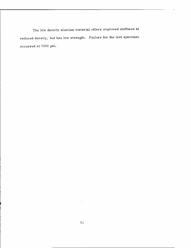
The low density alumina material offers improved stiffness at

reduced density, but has low strength. Failure for the test specimen

occurred at 7200 psi.

51

III. TENSILE STRENGTH

A frequent criterion to be used in the selection of composite

materials is the ultimate tensile strength of the material. Section A

contains an analysis of the tensile strength of uniaxially reinforced

fibrous composites. The validity of the analysis is tested by the

experimental program described in section B. The modification of

matrix properties to improve composite strength is treated in section

C

52

A. FIBER REINFORCED MATERIALS

1. Introduction

Composite materials consisting of a ductile matrix reinforced

by high-strength, high-stiffness fibers are materials of considerable

engineering practicality. The strength of such materials under tensile

loads has been studied theoretically with only limited success. An

analytical understanding of the failure of such materials is desirable,

not only to provide adequate design methods for existing materials, but

also to enable the definition of desirable characteristics of constituents

of composites for future applications. The problem treated here is the

failure of a composite, consisting of a matrix stiffened by uniaxially

oriented fibers when subjected to a uniaxial tensile load parallel to the

fiber direction.

The failure of a uniaxially stiffened matrix has been studied

previously by several investigators. Their findings are summarized

in L 16] . The simplest failure model treated assumes that a uniform

strain exists throughout the composite and that fracture occurs at the

failure strain of the fibers alone (e.g. L 17]). The effect of a non-

uniform strain distribution was studied in £l8] which suggests the in-

fluence of fiber flaws on composite failure. In [ 18] , 'failure occurs

when the accumulation of fiber fractures resulting from increasing load

shortens the fiber lengths to the point that further increases in load

could not be transmitted to the fibers because the maximum matrix shear

stress was exceeded. Thus, composite failure resulted from a shear

failure of the matrix.

53

In the present paper fibers are treated as having a statistical

distribution of flaws or imperfections which result in fiber failure at

various stress levels. Composite failure occurs when the remaining

unbroken fibers, at the weakest cross-section, are unable to resist

the applied load. Thus, composite failure results from tensile fracture

of the fibers. The composite strength is evaluated herein as a function

of the statistical strength characteristics of the fiber population and of

the significant parameters defining composite geometry. A numerical

example is presented for fiber-glass reinforced plastic composites

utilizing the existing data for tensile strength of glass fibers.

2. Description of The Model

The composite treated is shown in Fig. 25 and consists of

parallel fibers in an otherwise homogeneous matrix. The fibers are

treated as having a statistical distribution of flaws or imperfections

which result in fiber failure under applied stress. The statistical ac-

cumulation of such flaws within a composite material results in com-

posite failure. The computation of stress is quite complex when there

are discontinuous fibers present. These internal discontinuities result

in shear stresses which may locally attain very high values. An exact

evaluation of this stress distribution for the complex geometry of circular

cross section fibers arrayed within a matrix and for inelastic matrix

stress-strain characteristics appears to be unattainable from a practical

viewpoint. Such stresses were evaluated in [ 19] for idealized fiber

shape and without the effect of surrounding fibers. An approximate solution,

similar to that of [ 20 ] , but including the effect of surrounding fibers is

obtained herein.

54

In the present model, the extensional stresses in the matrix are

neglected relative to those in the fiber and the shear strains in the fiber

are neglected relative to those in the matrix. This approximation of

the model is considered appropriate for fibers which are very strong and

stiff relative to the matrix. In the vicinity of an internal fiber end, in

such a composite, (fig. 25) the axial load carried by the fiber is trans-

mitted by shear through the matrix to adjacent fibers. A portion of the

fiber at each end is therefore not fully effective in resisting the applied

stress. As the fibers are loaded, failure occurs at points of imperfection

along the fibers. Increasing load produces an increasing accumulation

of fiber fractures until a sufficient number of ineffective fiber lengths

combine to produce a weak surface and composite fracture. Basically,

then, the model considers fibers which fail as a result of statistically

distributed flaws or imperfections, and composites which fail as a result

of a statistical accumulation of such flaws over a given region.

At some distance from an internal fiber break the fiber stress

will be a given fraction, <P, of the undisturbed fiber stress cr . One a

may define this fraction of the average stress such that the fiber length,

0, over which the stress, a , is less than O may be considered in- a

effective. Thus, this ineffective length, 6 , is defined:

cr ( 6 ) = <pa a

Then, the composite may be considered to be composed of a series of

layers of dimension, 6 . Any fiber which fractures within this layer,

in addition to being unable to transmit a load across the layer, will also

55

not be stressed within that layer to more than the stress, O . The applied

load is treated as uniformly distributed among the unbroken fibers in each

layer. The segment of a fiber within a layer may be considered as a link

in the chain which constitutes the fiber. Each layer is then a bundle of

such links; and the composite is a series of such bundles.

The treatment of a fiber as a chain of links is appropriate to the

hypothesis that fracture is a result of local imperfections. The links may

be considered to have a statistical strength distribution which is equivalent

to the statistical flow distribution along the fibers. The realism of such

a model is demonstrated by the length dependence of fiber strength. That

is, longer chains have a high probability of having aweäker link than shorter

chains and this agrees with experimental data (e.g. [21 ]) which demonstrate

that fiber strength is a monotonically decreasing function of fiber length.

For this model, the link dimension is defined by a shear lag type

approximate analysis of the stress distribution in the vicinity of a broken

end. The statistical strength distribution of the links is then expressed as

a function of the fiber strength-length relationship, which can be experi-

mentally determined. Then these results are used in a statistical study

of a series of bundles of links to define the distribution of bundle strengths.

(Statistical techniques for a series of bundles have been studied in L 22 ]

for application to particle reinforced composites.) The composite fails

when any bundle fails and the composite strength is thus determined as

a function of fiber and matrix characteristics. These aspects of the

problem are discussed in further detail below.

56

3. Fiber Strength

The statistical distribution of link strength is obtained from the

fiber strength distributions. Consider links characterized by the dis-

tribution function f(a) and the associated cumulative distribution function

F(a) where:

(a) = j f(cr F(a) =] f(a) da (1) o

For n such links forming a chain which fails when the weakest link fails

the distribution function g(a) for the chain is defined by:

g(0) = nf(CT) [1 - F(0) ]n_1 (2)

That is, g (er ) der is the probability that one link fails between o and

CT + da (which is equal to f(a) da ), multiplied by the probability that all

n — 1 remaining (n - 1) links exceed O + der (which is [ 1 - F ( a ) ] ) and

failure can occur at any of the n links. From this, the cumulative dis-

tribution function, G (a ), for the fibers is obtained:

G (a ) = jg (a) da (3) o

.". G (a ) = 1 - C 1 - F (a) ]n (4)

The solution of the inverse problem is desired. That is, given

the fiber data, g (a ) and G (a), define the link data for a link length, Ö .

From eq. (4):

F(a) = 1 - [1 - G(a)] 1/n (5)

and thus from (1) and (5):

57

f(ff)=fi42L[i_G(a)](1^n)-1 (6> n

Consider fibers characterized by a strength distribution of the Weibull

type [23] : '

8 1 ß g(a) = L a ßop~ exP(-Laap) (?)

This form has been shown to characterize the experimental length-strength

relationship of fibers. Using equation (7) in (3) and (6) yields:

R 1 ß f(a)=aöScr exp(-aöcr ) (8)

where: L = nö

The constants a and ß can be evaluated by using experimental

strength-length data. To do this, consider the mean fiber strength, fff

for a given length which, is defined by:

CO

äf = f ag(<M da (9) c

Substituting eq. (7) into (9) and integrating yields:

äf = (Laf1/8 r(i+i) do)

A logarithmic plot of the available data for a as a function of L

will define the constants. Such a plot is presented in fig. 26 for the

data of [ 21 ] . The linearity of the data support the choice of the dis-

tribution function given by eq. (7). The constants are found to be:

-2 a = 7.74 x 10

ß =7.70

The constant ß is an inverse measure of the dispersion of material

strength. Values of ß between two and four correspond to brittle ceramics,

58

while a value of twenty is appropriate lor a ductile metal [ 22 ] . The

constant a, as seen from eq. (10), defines a characteristic stress level,

a~ 'P. For this distribution, a~ is 305 ksi. A more useful reference

stress level is mentioned in the discussion section.

4. Effective Fiber Length

The definition of ineffective length, Ö , involves the determination

of the shear stress distribution along the fiber-matrix interface. The

model used is shown in fig. 27 and consists of a fiber surrounded by a

matrix which in turn is imbedded within a composite material. The latter

has the average or effective properties of the composite under consider-

ation. This configuration is subject to axial stress and a shear lag type

analysis is utilized to estimate the stresses.

Load is applied parallel to the fiber direction. The fiber is as-

sumed to carry only extension and the matrix to transmit only shear

stresses. No stress is transmitted axially from the fiber end to the

average material. Shear stresses in the average material are considered

to decay in a negligible distance from the inclusion interface.

For equilibrium of a fiber element in the axial direction:

r da

T +-T- -—- = 0 (12) 2 dz

where T = shear stress in matrix material

CT = axial stress in fiber

For equilibrium of the composite in the axial direction:

2 2 2 a b £)v(- 2

a r a =a (13)

a

59

where a = axial stress in average material a

a - applied axial stress

The displacements in the fiber, u , and in the average material,

u , define the binder shear strain, y, as follows: a

u; - uf= (rb ■ rf>y (14)

Differentiating eq. (14) twice and using the stress-strain relations

yields:

i dCT 1 a da r - r ,2

If b f d T (15) E dz E, dz G, .2

a f b dz

where E = effective Young's modulus of the composite a

E = Young's modulus of the fiber

G, = shear modulus of the binder b

Differentiating eq. (13) and substituting the result and eq. (12)

into eq. (15) yields:

,2 d T n T = 0 dz

(16)

where

2G, r\ E£ (rb - rf) (rf) 1 + E-

a 2 2

r _ ru a b

(17)

The solution to eq. (16) is of the form

T = Asin h 77 z + Bcos hi z

The boundary conditions are:

T (o) =0

CTf W = 0

(18)

(19)

60

B = 0

A =

^ - 2 G CT r

b a

and

2 2 7?E (r -r ) (r -r ) cosh r\l

a b i a b

G, CT r sinh 77 z b a '

2 2 7)E (r -r.) (r -r, ) cosh y\ I

a b f a b

From eqs. (12) and (20):

- 2 ^ CT r E„

a £ f [E (r 2-r 2)+Er 2]

a a b ft

Consider r >> r, a b

. . r\ .2 2G2

ar E,

cosh 77z cosh Tjt

(20)

- 1 (21)

(22)

and from eq. (21):

CTE. cosh fj z cosh 77-t

The maximum axial stress is

O E, C£ (o)

I ->oo

(23)

(24)

Using the results of this elastic analysis, the stress ratio ,9 is

evaluated from the ratio of the stress at a distance 6 from the end of a

given fiber to the stress at the midpoint of a very long fiber. The stress

at a point at distance 6 from a fiber end is:

61

<TE

o£{l-ti) = .— cosh 77 (£-6) cosh 77 I

(25)

The fiber efficiency, <P , at this point is therefore defined by:

at (1-6) <P =

Of{o) 1 - cosh 77 Ö + tanh Tjl sinh 7] 6 (26)

i-t-*»

for large -t

tanh 7H = 1

2 1/2 .*. <p = 1 - cosh 776 + ( cosh TJÖ - 1) (27)

From which

cosh V 6

and

iJT

1 + (i - <p) 2 (1 - cp)

(v-1/2-i)-i ^ f ' G.

1/2

cosh

(28)

1 + ( 1 - (p) 2 (1 - <f> )

(29)

For the purposes of this analysis a value of V - 0.9 is considered, and

6 is evaluated for this stress ratio value. Thus, effective length is that

portion of the fiber in which the average axial stress is greater than 90%

of the stress which would exist for infinite fibers. Fig. 28 shows the

variation of ineffective length with constituent moduli for various fiber

concentrations.

The stresses upon which these results are based are shown in

fig. 29. It is clear that for many composites the matrix shear stresses

will exceed the elastic limit of the material. The point at which the elastic

62

limit is reached is indicated on each.curve of fig. 29 for a matrix shear

yield stress of one tenth the fiber strength. Since for high concentrations

most of the curves are above the elastic limit, further inelastic analysis

is required. Note also that the results of this shear lag model differ in

character from those of ref. 20. The difference is attributable to the

addition of the third or average material to the model.

The elastic analysis of this section has been extended to include

the effects of an elastic plastic binder. To do this, consider a region at

the fiber end in which the shear stress is equal to the shear yield stress,

T , thus: y

IT

a 2-(l- z) I- b < z £ I (30) z r f

Equation (12) applies for: 0 £ z £ I- b. The analysis for the elastic

region is unchanged except that the boundary conditions (19) are replaced

by:

T(o) = 0 (31)

T(l-b) = T

Substitution of (31) into (18) yields

T=T sin T?Z (32)

y sinTJ(^-b) <■"'

From eqs. (12), (13) and (32) it can be shown that:

0 = 1 JL cosh ^ (33) f . v2 „ r , ,2-, Tjr Sinh TJ(^-b) V ' r \ E

V Ef ' <i 63

for 0 ^ z s I - b

The length b is evaluated by assuring continuity of stress at z = I - b.

Thus from eqs. (30) and (33):

~ 2T 2T b y

v a ' f

For r > > r, this reduces to: a b

•M Vr

X- coth T)(t-h)

CTVf 1 b = 2FE~-T coth^-b>

y a

For b << -6

° Ef rf 1 b = TF-E ^r coth n*

y a (34)

Now the ineffective length can be evaluated, as defined by eq. (26)

by using eq. (33). It will be assumed and subsequently confirmed that:

6 > b. Large values of fiber length relative to all other fiber dimensions

will be assumed. The result is:

2 cosh r\ 6 = 1 + X

2X

where

X = cosh 7? 6 - (cosh2 r\ 6 - l)1'2

(38)

(36)

Simultaneous solution of eqs. (34) - (36) defines the inneffective length.

A limiting case is obtained for a rigid-plastic material. For a

uniform shear stress, the length, " ; required to obtain the full strength P

of the fiber is:

p 4T f y

(37)

64

Thus, for a composite of 400 ksi glass fibers in a 10 ksi plastic

binder, the plastic ineffective length is ten fiber diameters. This value

is about four times the appropriate elastic value.

5. Composite Strength

With the link length defined, [by eq. (29) for the elastic case;

eqs. (34) to (36) for the elastic-plastic case; and eq. (37) for the rigid

plastic case] and the link strength characterized by eq. (8), the com-

posite strength can be evaluated. First the strength of the bundle will

be determined, then the composite will be treated as a chain of bundles,

and weakest link statistical theorems will be applied. This leads to the

desired statistical definition of composite strength.

For a bundle of links, Daniels [24] has shown that for a large

number, N, of fibers the distribution of bundle strengths approaches a

normal distribution with expectation:

a =a [l - F (ff )] r5 m m

(38)

and standard deviation:

0 = a B m

F (o- ) [1 - F (a )] 1/2 N"1/2

m m

The associated density distribution function is

1 B v B'

exp i/)B JZir

1 / B B \

T B

(39)

(40)

The maximum stress is obtained by maximizing the total load.

Thus:

da a[l - F (a) ] (41)

o = a m

65

For links described by eq. (8): o

F(cr) = 1 - exp (-a Ö a ) (42)

Substitute (42) into (41):

— [aexP( -a6a ) ]ff=(y =0 m

/. a =(a6/3)" 1//? <43) m

From (38), (42) and (43):

ffB = M/3f 2/^ exp(--i-) (44)

From (39), (42) and (43):

[l - exp (- -=-)] exp (--J 4>B = ialß)- Uß 1,1 /Ml 1/2 M- 1/2 r)] exp (--H N

(45)

Layers characterized by eqs. (40), (44) and (45) may be con-

sidered as links in a chain and the weakest link theorems can be applied

again. Thus, applying eq. (2) to this case

X (<7 ) = n w (ff ) [ 1 - fl (ff ) ] n" (46) c c c

where ff is the composite failure stress, and X is the associated dis- c

tribution function.

The mode of this distribution is found by setting dX /da = 0.

This yields:

* — 1/2 , log log n + log 4ir ,„.,. ac -a B-0B(21ogn) +0 S S J*2 (47)

2(2 log n)

For composite dimensions large compared to fiber cross-section dimen-

sions, N>>1. Therefore:

66

and the statistical mode of the composite strength a #, is found to be c

ff.* = (a« ße) - Uß (48)

where a and ß are the constants defining the link strength and are de-

termined by experimental tests of fiber strength vs. length as described

previously. 6 is the ineffective length defined by a fiber shear stress

analysis and e is the base of natural logarithms.

The results of section 3 are used in eq. (48) to compute com-

posite strength as a function of the effective length. The predicted

composite failure stress is plotted in fig. 30 for the range of ineffective

lengths of one to one hundred fiber diameters. The range one to ten

generally corresponds to the elastic predictions and the range ten to one

hundred to the inelastic predictions.

Also shown in fig. 30 are the effects of variations in fiber character-

istics. Curves are presented to show the effect of an increase in the dis-

persion, as measured by a 10% change in ß and of a decrease in the

reference strength as measured by a 10% change in a" . For the

reference case plotted, the analysis also indicates that at failure the

mean number of fractured fibers per layer is less than 10% and that the

length at which the mean fiber strength equals the fiber stress in the

composite, at the most probable composite failure stress, is on the

order of ten ineffective lengths.

For a rigid-plastic representation of the binder material, failure

points for two different yield stress values are shown. Thus, for the

67

fiber data used, and for a yield stress of 10 ksi, the predicted strength

of a glass-plastic composite of 70% fibers by volume is 290 ksi. For

the same conditions binder yield stress of 20 ksi would indicate a com-

posite failure stress of 310 ksi. The effects of matrix characteristics

are more clearly defined by considering the elastic-plastic results ob-

tained in the latter part of section 4.

Mechanically, the elastic-plastic matrix material is characterized

by the initial elastic modulus, the yield stress, and the total strain to

failure. The influence of these three quantities on the tensile strength

of a composite consisting of an elastic-plastic matrix uniaxially rein-

forced with glass fibers is shown in fig. 31 in the form of shear yield

stress vs. elastic shear modulus required to achieve the specified

constant values of composite strength.

These results are obtained by selecting a fixed value of composite

strength, 6 *, and determining the corresponding ineffective length ratio

from fig. 30. For the elastic case the modulus ratio E /G and the

maximum shear stress, T , are determined from figs. (28) and (29) max

respectively. The asymptote for large shear moduli is found from the

rigid-plastic solution, eq. (37). For the region between the elastic

range, represented by the vertical portion of the curve, and the fully

plastic range, represented by the horizontal asymptote, the combinations

of values of shear modulus and shear yield stress which result in the

desired ineffective length are evaluated from eqs. (34) to (36). The

ultimate matrix shear strains required are not shown; however, they

68

are approximately parallel to the strength curves with decreasing strain

required for increasing composite strength.

The stress curves show the nature of property variations re-

quired to produce the maximum increase in composite strength. For

example, a composite containing an elastic-plastic matrix material

with a shear modulus of 150 ksi and a shear yield stress of 15 ksi will

be unaffected in strength by a ± 50% change in shear modulus but would

improve in strength with increasing shear yield stress and would also

require lower shear strain at failure; similarly, a matrix with a modulus

of 40 ksi and a strength of 30 ksi would be far more sensitive to modulus

changes than to strength changes. This is illustrative of the nature of the

results to be obtained from the existing failure model. Other types of

fiber and matrix materials need to be considered to complete the picture.

Fibers with different strength levels and strength gradients with respect

to fiber length, and matrices with monotonically decreasing tangent moduli

should be included. In any event, it appears that the qualitative evaluation

of the direction of improvement in constituent properties to obtain im-

proved structural composites can be achieved.

One of the reasons for the quantitative uncertainties can be seen

by exploring certain assumptions in the shear stress evaluation. First

of all, the idealization to a rotationally symmetric problem ignores the

variation due to the hexagonal or nearly-hexagonal array of nearest

neighbor fibers. Secondly, the selection of an average distance between

fiber and surrounding "average" material is not an obvious one. Although

69

the magnitude of the former problem cannot be assessed without the

solution of a complex elasticity problem, the latter can be studied by-

varying the average distance and determining the resulting effect upon

composite strength. The results of such a study are shown in fig. 32,

where the ineffective fiber length is plotted as a function of the average

matrix thickness expressed as a multiple of the fiber radius. The range

of abscissa values cover the range obtained by various reasonable idealiza-

tions for a fiber volume fraction of 0. 7.

6. Discussion and Conclusions

The analysis attempts to simulate what appears to be the physical

failure mode. An effort was made to include what were thought to be the

most important parameters influencing failure. Obviously, the model

will not provide accurate quantitative answers without further refine-

ments. It is expected, however, that the nature of desirable improve-

ments in constituent characteristics can be ascertained from the present

model. Such preliminary conclusions will be described below. The

shortcomings of the model include failure to consider fracture involving

parts of more than one layer, variation of ineffective length with stress

level, stress concentrations in fibers adjacent to failure areas and the

initial state of stress. Further, as the analysis indicates that short

fiber lengths may exist at failure, the shortcomings at short lengths

of the statistical distribution used for the fibers should be corrected.

That is, the limit of fiber strength with decreasing length should be a

finite value. Fiber experimentation can provide the data for such a

70

statistical model. On the positive side, however, the model represents

the constituents in the major functions of fibers carrying extensional

stress and matrix carrying shear stresses; it includes the effect of fiber

imperfections on fiber failure; and accounts for-the accumulation of

internal cracks which combine to produce composite failure. This latter

follows the concepts of Parratt [l8 ] who suggests the influence of flaws

and ineffective lengths on failure. The failure mode in the present

analysis, however, results from an accumulation of cracks rather than

from the existence of fully ineffective fibers. In fact the present results,

which indicate typical fiber lengths at failure which are an order of

magnitude larger than the ineffective length, perhaps explain the quan-

titative difference between the ineffective lengths of [18] and those of

[20] and this paper. The experimental results, described in the

following section, appear to be in qualitative agreement with the analytical

models.

The conclusions to be drawn from the analysis for the glass fibers

considered are as follows: Composite failure stress will be on the order

of short fiber failure stress, where short fibers are on the order of ten

ineffective lengths. Fiber strength levels appear to have the most direct

effect on composite strength. Fiber strength dispersion influences com-

posite strength and ineffective length of fibers has a significant effect on

strength. The latter is primarily influenced by the matrix characteristics

and an improvement of matrix strength appears desirable. The effect of

such changes upon the mode of failure remains to be considered.

71

The fact that these conclusions are not unexpected for glass re-

inforced plastics is encouraging, insofar as the possibility of fruitful

application of this analysis to consideration of other composites and to

the definition of "desirable constituent properties. Further, the actual

strength levels predicted for glass-plastic composites are higher than

those obtained experimentally. This could well be explained by the

additional damage incurred in fabrication after the state at which the

fiber tests of [21 ] were performed.

72

B. FIBER REINFORCED COMPOSITES - EXPERIMENTAL

The experimental study of the mode of failure of fiber reinforced

composites under a tensile load utilized specimens consisting of a single

layer of parallel glass fibers imbedded in epoxy. The specimen, as shown

in fig. 33, has a test section which is 1/2" x 1" in size and 0. 006" thick

and contains 90-100 parallel glass fibers of 0.005" diameter. The speci-

men is loaded in tension and observed microscopically during the test.

The design of the specimen was directed towards making this observation

possible, so that the nature of failure of fibrous composites could be

determined. In particular, the validity of the preceding analysis was to be

tested. (Similar test specimens appear to have been used with a somewhat

different goal in (25).)

Both visual observation and photographic observation were used

on all test specimens. A sequence from a typical set of photographic

data is shown in fig. 34. The load was applied parallel to the fibers.

Note again, that the fiber diameter is on the order of five times the

minimum distance between fibers. The first frame shows the specimen

at zero load. Polarized transmitted light has been used and at zero load

the fibers are dark and the plastic between fibers appears light. As the

load is increased, the fibers appear lighter, although this is not ade-

quately reflected in the photos since the lens aperture was changed

during the sequence. The difference between the unloaded specimen

photo and the next to the last photo in the sequence is four f stops, or

a factor of 16 on the exposure.

73

At less than 50% of the ultimate load, individual fiber fractures

are observed. Since the fractured fiber in the vicinity of the fracture is

unstressed, the color returns to the original dark color. Thus, breaks

appear as a short dark rectangular area with a thin white line across the

center. The length of this dark area is the ineffective length of the fiber,

(see section A)As the load increases, the fibers fracture at random

locations. Thus, although there are stress concentrations in the vicinity

of the breaks, the variation in fiber strength generally more than offsets

the effect of such concentrations. Hence, the breaks occur randomly rather

than cumulatively at the site of the initial break. The stress concentrations

cause a relative brightening at the highly stressed points of the fibers and

this effect appears on the latter photos in the sequence of fig. 34. Also

there are examples of breaks which were produced as a result of the

stress concentrations.

The specimen is shownin the last frame after fracture. It is not

clear that the actual fracture simulates the behavior of a three dimensional

composite and it therefore appears that the internal fractures prior to com-

posite failure are the primary data from these tests. The usefulness of

the test lies in the potential use of these results in conjunction with the

preceding analysis to predict and verify the direction of desired constituent

property improvements to achieve higher tensile strength composites.

The data for the specimen of fig. 34 are plotted in fig. 35. These results

are typical of the scatter of data points around the best fit curve. Such

curves for the series of test specimens described in table III-l are shown

74

in fig. 36.

TABLE III-l

Tensile Strength Tests - Series A

Spec. Gage Width Thickness Number Ultimate Number length of fibers load

(in.) (in.) (in.) (lb.)

1 1.10 0.499 0.0066 92 114

2 0.91 0.498 0.0060 93 84*

3 1.10 0.500 0.0067 93 111

4 0.90 0.502 0.0064 94 125

5 1.05 0.494 0.0061 92 116

6 1.02 0.500 0.0062 94 117

7 1.00 0.498 0.0062 93 116

8 1.07 0.503 0.0061 65*

9 1.03 0.490 0.0060 93 107

^Failure in grip section. Test data not used.

75

C. PARTICLE REINFORCED MATERIALS

The merit of a matrix material having enhanced stiffness and

strength properties compared to presently available plastic resins is

clearly evident from the analyses of composites. The first, most

directly available method of improving matrix properties appears to

be to make the matrix itself a composite. To this end a series of

specimens were fabricated to investigate the effect of the addition of

glass and alumina powder to epoxy resin.

The results bring up more questions than they answer. While

the stiffness of the particle-composite specimens were duly increased

by the additives to maxima of 1, 040, 000 psi for the glass particles

(10-200 micron characteristic dimensions) and 2,000,000 psi for the

alumina (325 mesh or finer), the strength and elongation of the resin

were degraded. A curious accompanying phenomenon was a marked

increase in viscosity of the glass-filled epoxy resin before curing. This

increase prevented the fabrication of specimens of greater than 30%

volume percent glass. With the alumina particles 48 volume percent

filler was attained without corresponding difficulties, but to reach the

maximum value of 62% a larger particle size (325 mesh) was required

than for all the other (900 mesh) alumina-filled specimens.

Increase in viscosity with addition of particles is certainly to be

expected. What is peculiar is the difference in character of the viscosity

change for the two particles used. For successful end use the resin

viscosity must be not substantially changed from the unfilled value, a

76

criterion that could be met by the alumina particles up to a content of

approximately 40 volume percent, but the question raised of the relative

importance of the many factors affecting viscosity is not answered by

the present re-sults.

Of much more interest and eventual importance than viscosity

(influence of the fillers in the fluid state) is the decrease in elongation

at failure of the filled specimens (influence of the fillers in the plastic

state). The influence in the elastic state is as expected. The Young's

modulus of the composite is improved substantially, just as desired,

and if this were the only effect the implications would be exciting.

Accordingly an explanation of the reasons for the poor performance in

the plastic range could be useful. Answers are needed to questions like:

1. Is the reduction of elongation dependent upon the material

used for the filler, - i« e. would a more compatible or better

bonding filler be less harmful?

2. Is the reduction of elongation dependent upon the geometry

of the filler, - i. e. would short, very fine fibers be better than

essentially spherical particles?

3. Is the entire problem a result of poor fabrication, - i.e.

were these first-attempt specimens unsound and can improved

fabrication technique restore the strength lost by adding the

filler ?

4. How would even the low elongation filled resins of these

tests behave as the matrix for a filament reinforced composite,

77

i. e. would the development of "fractures" in the matrix at these

elongations lead to premature failure of the composite?

The actual experimental results which generate all these questions

are presented in figures 38 and 39 without further discussion. The end

objective of an improved matrix material is worthy of continued

investigation.

78

IV. STRUCTURAL APPLICATION STUDIES

Although the bulk of this study has been devoted to determining

composite properties as a function of constituent properties, it is

important to emphasize that this is not an end in itself. Analysis of

basic applications must be performed to indicate the nature of desirable

material properties. For example, in the case of elastic constants, the

composites are anisotropic and no one simple property of an anisotropic

material adequately defines the efficiency of a structure using such a

material. Thus, it is necessary to perform a structural efficiency

type analysis treating generalized structures and loads. As an example,

stability of plates with oriented voids, subjected to in-plane compressive

loads are treated in section A. Also, the effective properties cannot be

used at the neglect of internal stresses. In the case of a practical

fibrous composite structures biaxial stiffening will introduce average

stresses in individual layers of a laminate which differ considerably

from the average laminate stress. Certain aspects of the internal

shear stresses are treated in section B as an example of this problem.

79

A. STABILITY OF PLATES WITH .ORIENTED VOIDS

A quite different measure of material effectiveness than its

extensional stiffness is its ability to carry compressive or shear

stresses without buckling. This measure must be applied with dis-

cretion, because there are many ways of changing the resistance of

buckling. For example obviously the least loss in buckling resistance

as material is removed to reduce the effective density occurs when

the material is taken from the centroidal plane of the plate, as in

sandwich construction. The problem we are examining here may be

considered applicable to the case in which a uniform material through

the entire thickness is desired, for one reason or another. We are

then seeking an answer to the question: Is there some angular direction

which gives a material uniformly lightened by oriented voids superior

resistance to buckling?

Method of analysis

Available equations from the literature of the buckling of flat

plates in compression and shear were used to calculate the variation

of buckling effectiveness with angle of void. The elastic constants

employed in the equations were calculated with the aid of (13) in similar

fashion to that employed for the stretching and shearing stiffnesses.

Essentially the result is that the bending stiffnesses are proportional

to the corresponding stretching stiffnesses, with account taken for the

effective Poisson's ratio applicable to the anisotropic plate.

80

Results

The results are summarized in figure 40, in which are plotted

normalized interaction curves for buckling of simply supported, infinitely-

long plates having voids longitudinally, transversely, and at 45 to the

edges. The normalizing factor is the equivalent weight solid plate. The

plate with longitudinal holes is shown to have the least buckling resistance,

that with transverse holes is better in shear and the same in compression,

and the one with 45° holes is better in compression and between the 0°

and 90° cases in shear. The differences are not substantial.

Conclusion and Discussion

While material with oriented voids does exhibit increased elastic

buckling resistance because of its lower effective density, the orienta-

tion of the voids is not important in the elastic range. Probably if any

criterion exists it is that the holes should in general be aligned in the

direction of principal stress, to delay as long as possible the onset of

plasticity.

81

B. LAMINATE SHEAR STRESSES

A second aspect of the failure problem which has been considered

is the study of shear stresses in a biaxially stiffened matrix; that is, a

material stiffened by parallel fibers in layers which are oriented alter-

nately in each of two directions. The case analyzed considers the two

layer directions to beatequal and opposite angles to the loading direction.

The stresses were determined using the methods developed in (26). The

results are plotted in fig. 41. The shear stress on planes parallel and

normal to the loading direction, T , is shown in fig. 41a, normalized

with respect to the applied stress, O , plotted as a function of the lamina

orientation angle, 9 . The principal elastic constants of an individual

lamina are indicated and are typical of glass reinforced plastic construction.

The directions parallel and normal to the fibers are considered to be the

weak shear planes and the stress on these planes, T^ > is therefore also

shown in fig. 41a. The question of failure due to shear stress involves

both the shear stress and the shear strength distributions. The maximum

shear stress, Tmax , is shown as the upper curve of fig. 41a. The effect

of material properties on the shear stresses acting in the principal directions

of each lamina, T , are shown in fig. 41b. The shear stresses in the

fiber direction are seen to constitute a moderately high fraction of the applied

axial stress and as such warrant further consideration as a mechanism of

failure.

82

V. CONCLUSIONS

The present study of the relationship of properties of composite

materials to properties of their constituents has been primarily concerned

with the evaluation of elastic constants and ultimate tensile strength of

fibrous composites. The effort has been primarily directed towards

the development of the basic theory governing the behavior of such

materials. Thus, by the use of variational principles of the theory of

elasticity, bounds on the elastic constants of fiber reinforced materials

have been obtained. For parallel fibers in an hexagonal array, the

bounds are exact. For parallel fibers in a random array, simpler

approximate expressions are obtained. These results can be used to

study the potential of fibrous composites utilizing any combination of

constituents.

The numerical results obtained, indicate that the effect of the

matrix upon most of the constants is far from insignificant. The possible

means of attaining improved structural composites thus include using an

improved fiber or modifying the binder material for a given fiber. Certain

aspects of the latter approach have been studied experimentally, with the

indication that loaded plastics are advantageous. One type of improved

fiber considered has been a non-circular fiber. It was demonstrated that

the transverse modulus of composites containing elliptical fibers of aspect

ratio four, can be almost doubled for only moderate fiber volume fractions.

These studies of elastic constants have demonstrated potential methods of

controlling any given elastic constant. It is now necessary to study certain

83

typical aerospace structural applications to define the desired type of

improvement of these constants and the relative merits of various

potential improvements. Preliminary structural application studies

have been performed. Extension of such structural efficiency studies

would permit the present results to be used to define guidelines for the

development of improved composite materials.

The second major aspect of the present work is the study of the

tensile strength of fibrous composites. The observed influence of fiber

imperfections upon fiber strength have been used as the basis of a model

which hypothesizes composite failure to be the result of a statistical

accumulation of randomly occuring fiber fractures. The study of this

problem involved an approximate treatment of the stress distribution in

the vicinity of an internal fiber fracture. These results enable the

evaluation of alternate possible modes of failure. An experimental

study utilizing reinforced plastic film specimens, observed microscopically

during loading, was undertaken to qualify the analysis and provide quanti-

tative evaluation of parameters in the analysis. The experimental results

correlated closely with the failure model utilized in the analysis and it

appears that the joint use of theoretical and experimental results can

define the desirable characteristics for improved structural composites.

Again, the analysis indicates that significant improvement in composite

performance can be obtained by variation of matrix properties as well

as by the obvious changes in fiber characteristics.

84

It appears that the proper understanding of the mechanics of

deformation and failure of composites can indeed contribute to the

attainment of the many potential improvements composites have long

been known to offer

85

ACKNOWLEDGEMENT

The authors wish to acknowledge the creative contribution of

Mr. R. K. Cole to the development of the experimental study of

reinforced plastic tensile strength described herein.

86

REFERENCES

1. Paul, B. , "Prediction of Elastic Constants of Multiphase Materials", Trans. AIME Vol. 219, I960, pp. 36-41.

2. Hashin, Z. and Shtrikman, S. , "Note on a Variational Approach to the Theory of Composite Elastic Materials", Journal of the Franklin Institute, Vol. 271, 1961, pp. 336-341.

3. Hashin, Z. and Shtrikman, S. , "A Variational Approach to the Theory of the Elastic Behavior of Multiphase Materials", Journal of the Mechanics and Physics of Solids, Vol. 11, 1963, pp. 127-140.

4. Hashin, Z. , "The Elastic Moduli of Heterogeneous Materials", Journal of Applied Mechanics, Vol. 29, Trans. ASME, Vol. 84, 1962, pp. 143-150.

5. Dietz, A. G. H. , "Design Theory of Reinforced Plastics", in R. H. Sonneborn "Fiberglas Reinforced Plastics", Reinhold Publishing Corp. , New York, N. Y. , 1956.

6. Outwater, J. O. , Jr., "The Mechanics of Plastics Reinforcement in Tension", Modern Plastics, 1956, p. 156.

7. Rosen, B. W. , Ketler, A. E. , and Hashin, Z. , "Hollow Glass Fiber Reinforced Plastics", Contr. NOw 6l-06l3-d, Final Report Nov. 1962, Space Sciences Lab. GE Co. , Philadelphia, Pa.

8. Hill, R., "Report on Theories of the Elastic Properties of Reinforced Solids", British Iron and Steel Research Association, Report D/19/62, 1962 (Unpublished).

9. Hashin, Z. , "Theory of Mechanical Behavior of Heterogeneous Media", Applied Mechanics Reviews (to be published).

10. Bishop, J. F. W. , and Hill, R., "A Theory of the Plastic Dis- tortion of a Polycrystalline Aggregate under Combined Stresses", Phil. Mag. Vol. 62, 1951, pp. 414-427.

11. Love, A. E. H. , "A Treatise on the Mathematical Theory of Elasticity", Dover Publications Inc. , New York, N. Y., 1944.

12. Goodier, J. N. , "Concentration of Stress around Spherical and Cylindrical Inclusions and Flaws", Journal of Applied Mechanics, Trans. ASME Vol. 55, 1933, pp. A 39-44.

87

13. Dow, N. F., Libove, C. , and Hubka, R. E. , "Formulas for the Elastic Constants of Plates with Integral, Waffle-Like Stiffening, NACA TR 1195, 1954.

14. Crawford, R. F. and Libove, C. , "Shearing Effectiveness of Integral Stiffening", NACA TN 3443, 1955.

15. Dow, N. F. and Gruntfest, I. J. , "Determination of Most Needed, Potentially Possible Improvements in Materials for Ballistic and Space Vehicles, General Electric Company TIS R60SD389, I960.

16. Machlin, E. S. , "Status Report on Non-Metallic Fibrous Rein- forced Metal Composites", Status Report, Contract NOw 61-0209-c, Sept. 1961.

17. Jech, R. W. , McDanels, D. L. and Weeton, J. W. , "Fiber Reinforced Metallic Composites", Proceedings of the 6th Sagamore Ordnance Materials Research Conference, August 1959.

18. Parratt, N. J. , "Defects in Glass Fibers and Their Effect on the Strength of Plastic Mouldings", Rubber and Plastics Age, Mar. 1960.

19. Sadowsky, M. A., "Transfer of Force by High-Strength Flakes in a Composite Material", Watervliet Arsenal, TR WVT-RR-6105-R June, 1961.

20. Dow, N. F. , "Study of Stresses Near a Discontinuity in a Filament- Reinforced Composite Metal:, Space Mechanics Memo #102, GE Space Sciences Laboratory, Jan. 1961.

21. Schmitz, G. K. , "Exploration and Evaluation of New Glasses in Fiber Form", Bi-Monthly Progress Report No. 4, Solar Report RDR 1266-5, August 1962.

22. Gucer, D. E. , and Gurland J. , "Comparison of the Statistics of Two Fracture Modes", Journal of the Mechanics and Physics of Solids, pp. 365-373, 1962.

23. Weibull, W. , "A Statistical Distribution Function of Wide Applica- bility", Journal of Applied Mechanics, Sept. 1951.

24. Daniels, H. E. , "The Statistical Theory of the Strength of Bundles of Threads", Proceedings of the Royal Society, p. 405, 1945.

25. Bouc, C. A. , "Microscopic Study of Mode of Fracture in Fila- ment Wound Glass Resin Composites", T&AM Report No. 234, University of Illinois, Nov. 1962.

26. Rosen, B. W. , "Elastic Constants of Laminates of Orthotropic Plates", Space Mechanics Memo #112, General Electric Company, June, 1962.

89

a.) HEXAGONAL ARRAY

b.) RANDOM ARRAY

Figure 1. Fiber Arrays Considered for Elastic Moduli Analysis

90

AX, Z

BINDER

FIBER

VOID

a.) SECTION

b.) END VIEW

Figure 2. Composite Cylinder, Notation for Elastic Moduli Analysis

91

<75 3.0

ID O

* 0J LU

CO =) _l

8 2.0

CO CD z: O >- Ld CO ct ÜJ > CO

< l-

1.0

0

Ef =10.5X10

Eb =0.4X10

uf =0.20

vb =0.35

0.2 0.4 0.6 0.8 .0

GROSS FIBER VOLUME FRACTION, v t

Figure 3. Bounds on the Effective Transverse Young's Modulus for Solid and Hollow Glass Fibers in a Plastic Matrix (Parallel Fibers, Random Arravl

92

23(r)

'I

0 0.2 0.4 0.6 0.8 GROSS FIBER VOLUME FRACTION,vt

Figure 4. Bounds on the Effective Transverse Poisson's Ratio for Solid and Hollow Glass Fibers in a Plastic Matrix (Parallel Fibers, Random Array)

93

Kr)

0 0.2 0.4 06 0.8 GROSS FIBER VOLUME FRACTION, vf

Figure 5. Effective Shear Modulus in the Plane of the Fibers for Solid and Hollow Glass Fibers in a Plastic Matrix (Parallel Fibers, Random and Hexagonal Array)

94

10 r

00 « a. o

O

Ef = 10.5X10

Eb = 0.4Xl0'

i/f = 0.20

i/b=0.35

a = 0

0 0.2 0.4 0.6 0.8 1.0 GROSS FIBER VOLUME FRACTION ,vt

Figure b. Effective Longitudinal Young's Modulus for Solid and Hollow Glass Fibers in a Plastic Matrix (Parallel Fibers, Random Array)

95

0.4 r

T 0.3 -

o

< Q:

in

o CO CO o Q_

Q

t o.

a =0.8

Ef = 10.5 x I06

Eb = 0.4 x |06

i/f = 0.20

vb = 0.35

i i ii 1 0 0.2 0.4 0.6 0.8 1.0

GROSS FIBER VOLUME FRACTION, vt

Figure 7. Effective Longitudinal Poisson's Ratio for Solid and Hollow Glass Fibers in a Plastic Matrix (Parallel Fibers, Random Array)

96

''K ^ / SJ>

' /// ' sT / /

in / ro / // / o / ' ' / ii / ; / / *-

^ / /

-

_ (/> «0 a. CL

<0 (0 O Ü

X X in — ro sl- in ro O O O O II II II II XI X) <♦- x>

>

1

UJ LÜ

i

-

in in

in U <u

rO

o k TO ra ni

i—i

Ü

£ 0

.—1 1—1 0

■ K 00 M:

o

's

Modulu

s fo

dorn

Arr

ay

)

CO Ö M R

O o 3 Pi 0 ^

\- en < <D h cr in <u

CO 0) -H > h

_J 2 -i Q

R <U ro i—i

sr <

s T

r ara

l

o tr > PH

Lt in £ X CD — m !n u_

the

E

c M

at

C\J a -a o

e 8.

B

ounds

o

in a P

ias

o u

!sd9oi'|3tSnnnaoi^l SONDOA 3SU3ASNVai h

97

I.Or

5

- 0.8-

< en if) •z. o if) in o Q_

Lü in (T Lü > if)

<

0.6-

0.4

0.2-

0

- vb = 0.3 Eb = 0.4 X I06psi

Ef = 10.5 XI06psi

- vb = 0.35

- y/V\ r=0.35 ]

/

1 i i i i

0.2 0.4 0.6 0.8

FIBER RADIUS RATIO, a

.0

Figure 9. Bounds on the Effective Transverse Pois son's Ratio for Hollow Glass Fibers in a Plastic Matrix (Parallel Fibers, Random Array)

98

to to o O X X in in

to <fr *• ro ro o o O O O II II ii ii n X> XI «^- XI «»-

> ÜJ UJ ft ft

o £ o X o r- • r-l

- o cvj

U • H

in CO

i—i

OH

00 ctf sr

00 <t o 0

ö > m

Cfl

Ö 2 3

#» O 3 T3 o

o 0

"-in < en

CD oo So ÜL

ÜJ

ß

0

Q ^ <u < _)

_l o CD u <u >

QL > en

ß

WCM Q cti

m — <&. — — o H

LLO > CD >

CO CD H

+■> 0 CJ X CJ «^

MH

w r—C

1

00 CU

CM CM O ß

0 O ,—1

O en CU

-d 1—1

a ni 0 ^ 0 CO

CQ Ä

o r—i

O O CD ^1

3 00

!Sd9oi4j3 *3nna0IAI S9N00A 3Sä3ASNVUl (n

99

Vb = 0.3

< a: (D

o if) in O Q_

LU (/) a: Ld > in

< cr

.0

0.8-

0.6-

0.4-

0.2-

0

0

1.0 0.2 0.4 0.6 0.8 FIBER RADIUS RATIO, a

0.028 0.112 0.252 0.448 0.700 VOID VOLUME FRACTION,V0

Figure 11. Bounds on the Effective Transverse Poisson's Ratio for a Plastic Matrix with Parallel Circular Holes

100

IOOI-

w50 a. O

*1 LLI

co 20 Z> _J Z> O O s 10 CO CD ■z. Z>

<

Q Z> H O

2-

Eb £ I.OxlO6

"b = 0.3

vf = 0.3

vb = 0.3

100

YOUNGS MODULUS OF FIBERS, Ef, I06 PSI

Figure 12. Effective Longitudinal'Young's Modulus of a Fibrous Composite as a Function of the Young's Modulus of the Fibers

101

o o

s o

8

lus

of

a F

ibr

f th

e F

ibers

in 3 O Ü. 0 ra

o »o

ng

's

M

Modulu

C\J _ *•-

ÜJ You

ng's

^ X 3 CO

m o Cd £ i* UJ >> cp

o CD s * Ö +J U_

£ n LL. H r o <D o

to > ■•-'

-) o s _l -) £ fa

U) Q W cti O <" Cfl

2 •B ri CO O .H

0] e> -> o >-

- CM

a

o o PQ O

ID

Ü0

fa

ISdgOl' ra'smnaow SONOOA 3SU3ASNVUI

102

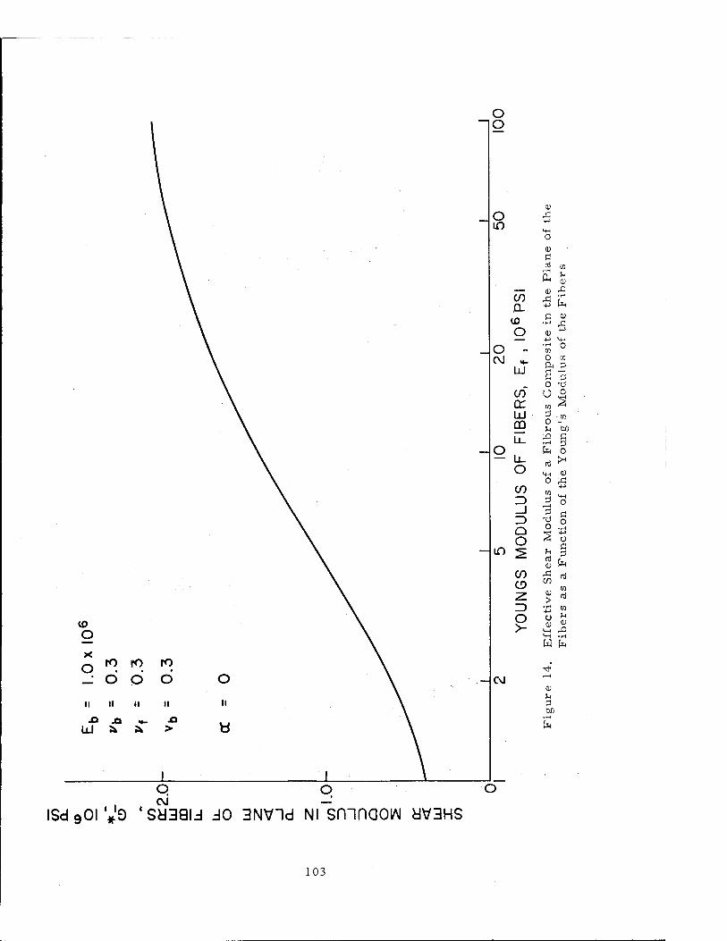
ID O

ro ro _• o O o o II II ii II II

LU ^ > «

o CM

o o

0)

o ^ in

e P

lane

of 1

bers

CO 6 £ 0- to •^ ,fi O <u ^ -^ +J m

o » —' 0 en C\J

ÜJ 0 in

£ -3 o -d

CO O ° en ^ tr

Ijj 5 ;™ m O - h 00

u_ X> fi

o fe o Ll_ o

o ^ CO 4-)

=> i " _J 3 fi Z> 'S o Q

ear

Mc

Funct

i

O m ^

CO £ «i o in

z £ * ID ■■Ö s° O u h

>- MH ,0

CM

isdgoi V9 'sysaid do 3Nvid Ni sninaoiAi UV3HS

W h

■tf

00

tu

103

5.01-

4.0

3.0 TRANSVERSE MODULUS,E2

(psi X I0"6)

2.0

.0

0 I

AXIS OF LOAD " AND STIFFNESS E2

AXIS OF PRINCIPAL STIFFNESS E| >

Ef Eb 10.5 0.4XI06psi 16.0 0.4 10.5 0.8

1 0.5 0.6 0.7 0.8 0.9

INCLUSION VOLUME FRACTION, Vf

Figure 15. Effect of Transverse Cylindrical Inclusions on the Effective Young's Modulus of a Stiffened Elastic Matrix

104

o 1 I

o 1

1

6 1

o o

1

o 1

1

o 1

o o Ö

1

1

Ö 1

o o

1

o 1

1

o 1

o o

1 1

o 1

1

o o

(a) (b)

(c)

Figure 16. Model Used for Analysis of Oriented Voids

105

1.0 F,

1.3

.8

.6

■I. max

.4 -

/3=/3'=-5

AXIS OF J \ PRINCIPAL-^/ \ STIFFNESS E|/ \

keTo

0

STIFFENING DIRECTIONS

AXIS OF LOAD AND STIFFNESS Ex

/*=0.3 X = 0 ß--0

15 30 45 60 75 90

ö, deg

Figure 17a. Variation of Principal Stretching Stiffness with Angle of Orientation of the Holes for Various Values of Transverse Effectiveness

106

1.0

.8 -

max

AXIS OF ./ PRINCIPAL—n STIFFNESS E|/

STIFFENING DIRECTIONS

AXIS OF LOAD AND STIFFNESS Ex

/*=0.3 X = 0 £' = 0

0 15 30 45 60 75 90

0, deg

Figure 17b. Variation of Principal Stretching Stiffness with Angle of Orientation of the Holes for Various Values of Transverse Effectiveness

107

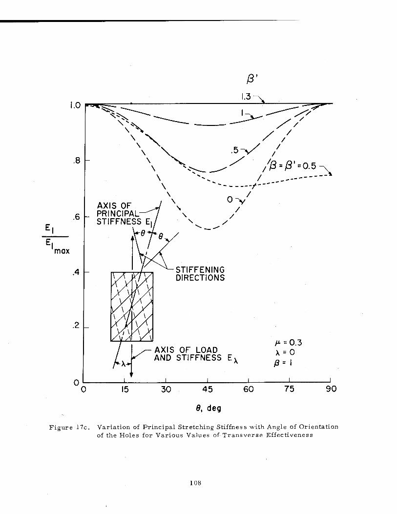
ß' 1.3-

.8

\ *

\ v \

/

/ -v

/ 7

.6

max

.4

w \ \ \ \

AXIS OF J \ PRINCIPAL-^/ \ STIFFNESS E|/

.5 /

//3 = /3' = 0.5 /

\

"- /■

/ /

y

STIFFENING DIRECTIONS

AXIS OF LOAD AND STIFFNESS Ex

^=0.3 X = 0 ß-~ I

15 30 45

0, deg

60 75

I\

90

Figure 17c. Variation of Principal Stretching Stiffness with Angle of Orientation of the Holes for Various Values of Transverse Effectiveness

108

ß

1.0

.8 _/3=/3'=o.5

!. max

AXIS OF J PRINCIPAL-^/ STIFFNESS E|/

kerB

STIFFENING DIRECTIONS

AXIS OF LOAD AND STIFFNESS Ex

45

0, deg

60

^ = 0.3 X = 0 /3'=l.3

75 90

Figure 17d. Variation of Principal Stretching Stiffness with Angle or Orientation of the Holes for Various Values of Transverse Effectiveness

109

1.0 r

.8

.6

max

AXIS OF J, L PRINCIPAL.—"/ N

STIFFNESS E|/ \

0

STIFFENING DIRECTIONS

AXIS OF LOAD AND STIFFNESS Ex

M=0.3 0 = 0° ß--0

0 15 30 45 60 75 90

X, deg

Figure 18a. Effect of Variation of Transverse Shearing Effectiveness on Stretching Stiffness

110

1.0

.8

max

AXIS OF J » PRINCIPAL-^/ N>. STIFFNESS E|/

STIFFENING DIRECTIONS

AXIS OF LOAD AND STIFFNESS Ex

^ = 0.3 0 = 15° /3 = 0

15 30 45

X, deg

60 75 90

Figure 18b. Effect of Variation of Transverse Shearing Effectiveness on Stretching Stiffness

111

1.0 r-

.8

.6

max

AXIS OF PRINCIPAL STIFFNESS E

0 0

STIFFENING DIRECTIONS

AXIS OF LOAD AND STIFFNESS E

H- =0.3 0=30° ß--0

30 45 60

X, deg

75 90

Figure 18c. Effect of Variation of Transverse Shearing Effectiveness on Stretching Stiffness

112

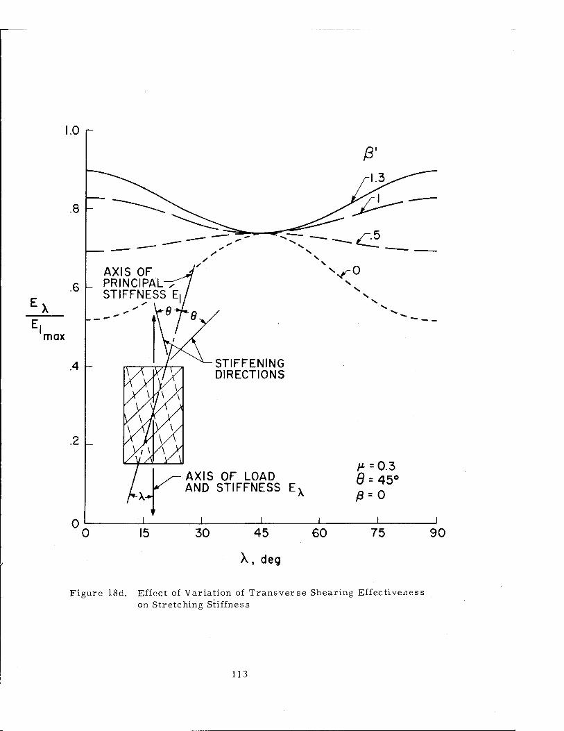
.8

.6 AXIS OF J

L PRINCIPAL^/ STIFFNESS E|/

max

.2

0

0'

STIFFENING DIRECTIONS

AXIS OF LOAD AND STIFFNESS Ex

0 30 45

X, deg

60

M=0.3 0 = 45° ß--0

75 90

Figure 18d. Effect of Variation of Transverse Shearing Effectiveness on Stretching Stiffness

113

ß= 0 or 1.0 /3'= 0 or 1.0

Figure 19a. Effect of Variation of Both Transverse Shearing and Stretching Stiffness on Stretching Stiffness

114

.0 R

#, deg 45

.8

.6 -

max

.4 -

0 0

AXIS OF J PRINCIPAL-^/ STIFFNESS E|/

kere

STIFFENING DIRECTIONS

AXIS OF LOAD AND STIFFNESS Ex

15 30 45

X, deg

60

j8=.5

P.*

75 90

Figure 19b. Effect of Variation of Both Transverse Shearing and Stretching Stiffness on Stretching Stiffness

115

.0

.8

max

AXIS OF J PRINCIPAL-^/ STIFFNESS E|/

STIFFENING DIRECTIONS

AXIS OF LOAD AND STIFFNESS Ex

M = 0.3

45 60 75 90

X, deg

Figure 19c. Effect of Variation of Both Transverse Shearing and Stretching Stiffness on Stretching Stiffness

116

i.O

.8

max

AXIS OF J PRINCIPAL-^/ STIFFNESS E|/

STIFFENING DIRECTIONS

AXIS OF LOAD AND STIFFNESS Ex

45 60

X, deg

H---0

£'=.5

75 90

Figure 20a. Effects of Variations in Poisson's Ratio on Stretching Stiffness

117

.0

.8

I. max

AXIS OF J PRINCIPAL^"/ STIFFNESS E|/

0

STIFFENING DIRECTIONS

AXIS OF LOAD AND STIFFNESS Ex

0 15 30 45 60

■/*s.3

fr*

75 90

X, deg Figure ZOb. Effect of Variation of Both Transverse Shearing and Stretching

Stiffness on Stretching Stiffness

118

.8

.6

max

.4

AXIS OF J PRINCIPAL-^/ STIFFNESS E|/

STIFFENING DIRECTIONS

AXIS OF LOAD AND STIFFNESS Ex

H---.5

#■5

j i

0 15 30 45

X, deg

60 75 90

Figure 20c. Effects of Variations in Poisson's Ratio on Stretching Stiffness

119

0 ^ 8 ± 45

AXIS OF LOAD AND STIFFNESS Ex

^=0 /3=0 or 1.0 /3= 0 or 1.0

X, deg

Figure 2 la. Combined Effects of Variations in Angles of Orientation of Holes, Transverse Effectiveness, and Poisson's Ratio on Stretching Stiffness

120

j3'=o

Figure 21b. Effect of Variation of Both Transverse Shearing and Stretching Stiffness on Stretching Stiffness

121

X, deg

Figure 21c. Combined Effects of Variations in Angles of Orientation of Holes, Transverse Effectiveness, and Poisson's Ratio on Stretching Stiffness

122

1.0

.8

.6

max

AXIS OF J PRINCIPAL-^/ STIFFNESS E|/

STIFFENING DIRECTIONS

AXIS OF LOAD AND STIFFNESS Ex

15 30 45

X, deg

60

^ = 0.5 ß=0 ß= 1.5

75 90

Figure 21d. Combined Effects of Variations in Angles of Orientation of Holes, Transverse Effectiveness, and Poisson's Ratio on Stretching Stiffness

123

#, deg

.8

.6

max

/ \ / \/ /

AXIS OF / PRINCIPAL STIFFNESS E

0

STIFFENING DIRECTIONS

AXIS OF LOAD AND STIFFNESS Ex

^=0.5 ß=\ ß'-0

0 15 30 45 60 75 90

X, deg

Figure 21e. Combined Effects pf Variations in Angles of Orientation of Holes, Transverse Effectiveness, and Poisson's Ratio on Stretching Stiffness

124

1.0

.8

■I max

#, deg 45

AXIS OF J PRINCIPAL-^/ STIFFNESS E|/

STIFFENING DIRECTIONS

AXIS OF LOAD AND STIFFNESS

45

X, deg

60

/* = 0 0=0 /3= i.o

75 90

Figure 2 If. Combined Effects of Variations in Angles of Orientation of Holes, Transverse Effectiveness, and Poisson's Ratio on Stretching Stiffness

125

1.0 r 0, deg

.8

.6 PRINCIPAL- STIFFNESS E|

max

.2 _

Figure 21g.

STIFFENING DIRECTIONS

AXIS OF LOAD AND STIFFNESS Ex

15 30 45

X, deg

60

H---0

ß'-0

75 90

Combined Effects of Variations in Angles of Orientation of Holes, Transverse Effectiveness, and Poisson's Ratio on Stretching Stiffness

126

■iff UP? jHfcw*r "%sif

f Gage point \,f- J

***(»«»»H

Inclusion Aspect Ratio = 1 Inclusion Aspect Ratio = 4

Young's Modulus = 0. 98 x 10 psi Young's Modulus = 1.77 x 10 psi

Figure 22. Test Specimens for Influences of Fiber Shape on the Effective Transverse Composite Modulus

127

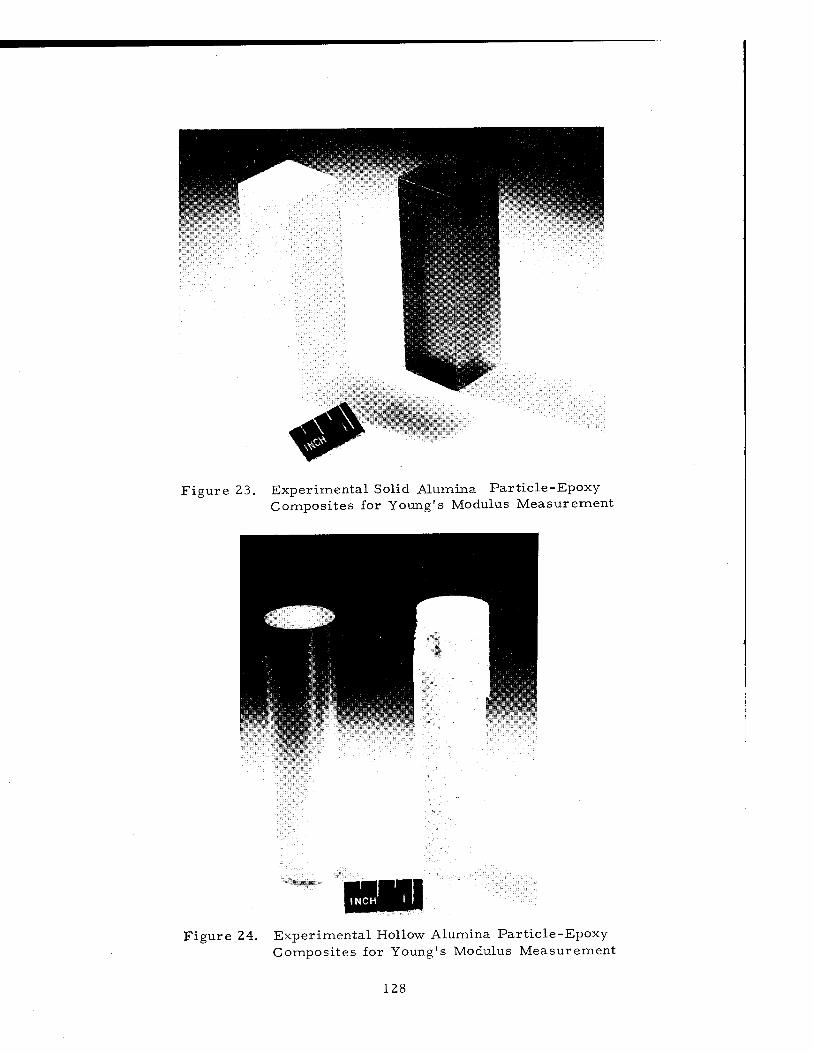
Figure 23. Experimental Solid Alumina Particle-Epoxy Composites for Young's Modulus Measurement

Figure 24. Experimental Hollow Alumina Particle-Epoxy Composites for Young's Modulus Measurement

128

\t t t t \

+> a

\ i i i j \

Figure 25. Fiber Reinforced Composite - Failure Model

129

o o

o in M

O

0

o u

E o

I h- CD Z UJ

M fi 0) !^

+-> CO

■l-l

fn a 4)

CD a o

in ß

1 1 1 1 o o o o o o o o o o m <fr rO OJ —

!SM 'SS3U1S BUniVd

o

u d M

130

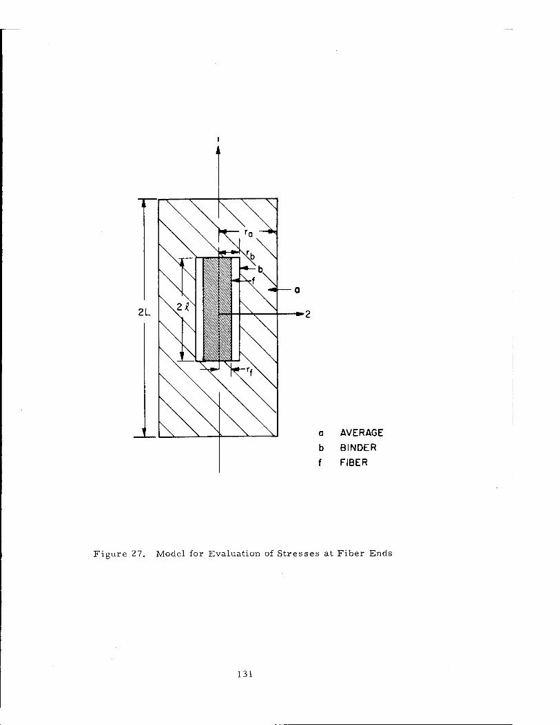
a AVERAGE

b BINDER

f FIBER

Figure 27. Model for Evaluation of Stresses at Fiber Ends

131

MODULUS RATIO,E|/G2

Figure 28. Ineffective Length of Fibers in Composites

132

a] in <P U

u 0)

w <u u n!

H-l

1 S-i <U

£>

fa

nj

M 0)

M •r-t

^ / XDUU j. 'oiiva SS3Ü1S UV3HS lAiniAIIXNM

133

L

O O

X3 \ CO

g"

UJ _J

LÜ > H O UJ u_ u_ LÜ

o <0.

o

— 1 o -|oa. o

CO. 1 o

o o

o d

in en D

+-> W IP u 3

tu

en O

a o u

in

i—i

PH

in rti

Ü

o

ni

o

o o o o f^- (X)

o o in

o o o

o rO

O O CM

o o

is*' °-o'ss3ais 3annvd

134

CO

CO CO ÜJ a: cö 100

< UJ i CO

cr UJ Q z CD

10

350 KSI

325 KSI

o- = 300 KSI

10 50 100

BINDER SHEAR MODULUS ,Gb ,KSI

500 1000

Figure 31. Influence of the Shear Modulus and Shear Yield Stress of an Elastic-Plastic Binder Upon the Strength of a Glass-Fiber Reinforced Composite

135

\ CO

o

a:

UJ i- ÜJ

<, Q

X I- o z UJ _l UJ > I- a u_ U_ UJ

a: UJ m

0 1.0 2.0

EFFECTIVE BINDER THICKNESS TO FIBER RADIUS RATIO, a/rf

Figure 32. Effect of Volume of Binder Assumed Acting with a Fiber Upon the Fiber Ineffective Length

136

A t

PLASTIC

-GRIP SECTION

-TEST SECTION FIBERS

-GRIP SECTION

a. PLAN VIEW

b. SECTION A-A

Figure 33. Tensile Failure Test Specimen

137

UNLOADED;

r'£it^#33r.v«ia3i

i^-^--■afj« **•:■!

: IT?*1. '^T";*'«««!?*?!

7.2%

MMMRMNR hm I ™^^B

' -^ss .■•*.■"♦■*■.--»". .»" • ."*itf?*a}«*.'i*n.\f**'* .*-*"?'*v..*

4'5.! % •' Figure 34a. Typical Sequence of Photographs of Tensile Failure

Specimen Showing Distribution of Fiber Breaks Prior to Failure (Specimen A-7)

138

lüipli

W^^^^^^^^^^^^^^^^^^^^m^^M^^^^^^m^M

52.9 %_

I

^^^^B^^^^^^^feft^^s §sÄS£|ggpggmgggps^&i

p*mwm*^j^^uy*;>-»^* .iVj

rt-v^uRr:.):^

"■* -.---=■ zu11? J1-Z--X

•Tr-ir,.-,.-^-« SB SS.-?..-. ■•SS^T*-T=?S "5 ■""^■■l "■-'■'■■""jj —^=r-^.*;. SÄS -rrrrr:——-JZLI- rrr-:-r.—. T—.—

rlfH^rr. ü §B9

„„■ •;;. - ^g^^^^^^-gtl „■,s:r„. I^Wflf^

äE£ ̂ iJStttffsesSsFgTlJ s .r'ib -srri-ria ÜJ!;;jwji^ji,. i ".-«T*':—"*—■ AMT*-** ^T^^F^^r^^^**^1

' ia"2!''?V'~X yw«fl'yaiS£S|ifMisr' T—--::*.--:~-rr

assS &£S ai.w.ü^S Tr-r; Äff—' -- -

«!V J52 -...., __ _. __ _ ;T"J3»«:;"

-•r:r"T £=~3 •-"'S» «M-Ä3i«i «■»tfißsssr:;-. .1 Hä

60.4%

Mfj'Wmjpjff i Ji» I II —»»iHMPj jf V • ■Vji%»***"wS,B'l*

64.9%;i/^"-''T-*:'-:'''' '

Figure 34b. Typical Sequence of Photographs of Tensile Failure Specimen Showing Distribution of Fiber Breaks Prior to Failure (Specimen A-7)

139

69.0%

■He

■ i -7 "2 c 0/

Wiimawg

78.3%

Figure 34c. Typical Sequence of Photographs of Tensile Failure Specimen Showing Distribution of Fiber Breaks Prior to Failure (Specimen A-7)

140

ft'"- —*WKOrr— •rummmg*

9 1.0%

Figure 34d. Typical Sequence of Photographs of Tensile Failure Specimen Showing Distribution of Fiber Breaks Prior to Failure (Specimen A-7)

141

99.0 %m^^m

mm***? ::".'.i

, ...S»a-»v.>-,j

»BTr::.-.-. ■■* ■■-■■•

Figure 34e. Typical Sequence of Photographs of Tensile Failure Specimen Showing Distribution of Fiber Breaks Prior to Failure (Specimen A-7)

142

FRACTION OF ULTIMATE LOAD

Figure 35. Number of Fiber Breaks in Specimen A-7 as a Function of Applied Load

143

0 10 20 30 40 50

NOMINAL FIBER STRESS

60 70

Figure 36. Number of Fiber Breaks as a Function of Nominal Fiber Stress for Series A Specimens

144

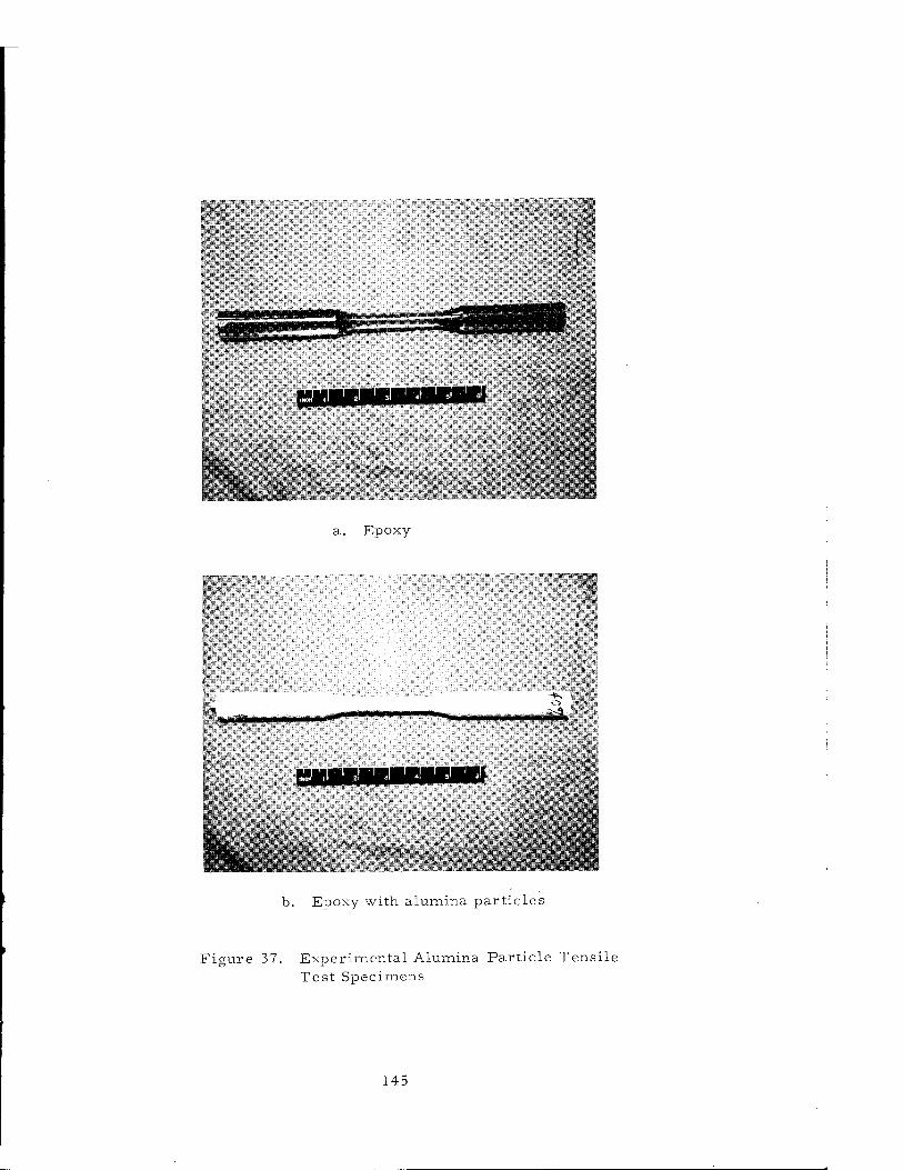
«»dumm»"'"»"1"'*'1

a. Epoxy

isi

hv ";«' SHHB^ vl.fi.

tiill«ll n> ■■Mail!

b. Epoxy with alumina particles

Figure 37. Experimental Alumina Particle Tensile Test Specimens

145

en

O

u «j >

h

CO

CU

Pi

X o

w o CO u u <u - -Ö

CO [J

o

SH

cd

u

CM

<

aj <i> U

+-> 10

C UJ <l) U) C) CD u M <\1

CO PH

. 00 en

<o u 3 ao

fa

CO 00

IS>4 'SS3U1S 31ISN31

146

1.5

in *:

to O

LU

if)

_l

Q O

^0.5: -z. Z)

?

AVERAGE OF TEST POINTS

0

m

55 r m

■JO m

10 o H

C/)

0 0.1 0.2 0.3

VOLUME FRACTION OF GLASS PARTICLES,Vg

O

s

> E m

0 * c

Figure 39. Tensile Properties of Glass Particle Reinforced Plastic Composites

147

N

SHEAR 2

xyvoids N

^solid

0 0

HOLE ORIENTATION

TRANSVERSE

LONGITUDINAL-

COMPRESSION Nx -A

N*solid

Figure 40. Normalized Interaction Curves for Buckling of Infinitely Long, Simply Supported Flat Plates of 40% Oriented Voids Under Combined Compressions and Shear

148

SHEAR STRESS

RATIO-^

-=F=0.2 El E2 -=0.5

max

AXIS OF

DIRECTION OF jL0AD' °" STRESS, T|2X^Ö/

DIRECTION OF STRESS

VTxy

0 10 20 30 40 50 60 70 9 deg.

0 90

Figure 41. Shear Stresses in Biaxially Stiffened, Filament-Matrix Composites

a. Effect of geometry

149

0.8 r

0.7

0.6 -

SHEAR °5

STRESS RATIO, T|2 0.4 -

0.3 -

0.2 -

0.1 -

2/E| G,2/E|

'/4

0.4 0.4

0.2

z/2|='/4

0 10 20 30 40 50 60 70 80 90 0, DEC.

Figur-e 41. Shear Stresses in Biaxially Stiffened, Filament-Matrix Composites

b. Effect of lamina properties

150 NASA-Langley, 1964 CR-Jl

< z

< z

u < in < Z

.i to -r< in

in

C C 3 O

rt bu £• rt E 0) bOX) C £ £CJ»3

i 'in «■=8,

"O OJ O

* .2 t! 3 «t « o h 3

« 0) e

S| o *•§ 5>rt c E S o .5 g

« p » -3 u •"

56a»« m > ,3 si

3-S-o <" w f- 3 ° 01 c

u a 2 .s 2 "8

_ rt 'S S- " . c c -o p m

" " -= o Ä in m

o " -* £2 o> o Bah

Ü S.5 u_ 5 a o ~ « = ° ä QJ bo _ e c

o a a ">5 S in ^ a

13. "O "* a " in »r « •o.

" 5-2 bG —» fc«

rt a

a - is 'S, c E o o .5 §|3 ^ (H -■

5 8 0J

S 33

«I • iri tu

o> •"" >, J5 i»3 a c c w s s o S «

1 01 91 C >> a, bo

JH M « _•

" »-€, j>>f w a; c o r a o c g in bD O " (U = a « a '3 J d I« uT] ^ 03t,ma>-'^t3c>aS

S-a gaa>-5?mrtP = ȤE

S a« Bifi »5-c s °-°S ° .Srtao.3MinoCD.uoCu

e U < < Z

CMS

a"SI 01 rt P •Me« oca

I Sis u 08 u

in u _ c c 3 O 0) « t. is 5 =

.i to a ■

rt bo "- rt £ 0) bOJD C (L . J: c a 0) 3

!x) bog- c.

I« _ E3

£3 e - p in

.3 <"

- a a £ g 01 *-■ A .

o 0..2

£ x: 3

,^ H rt >, is

in c rt

c rt i-H c t/j

QJ

a in 3 10

0 0 T1 t.

O

< !-* <J in

< Z

a s rt rt rt 0

rt g" a>

c K ">'^

■£:§^ rt in £

■SO« rt a, o ■o c in

£ o -a

g^ S3

o

<u £

a o

a c a. ai

o| m o

in

I»! Sog o M u

0 S V ss -

■2 in -o

_ tt) — .5 X) in •

OB«

J«J cj bo a

-5 c -

in £ ■a >

J2 o ■

1 x: ^ " -J-

IH m - o OJ

a ^ in

T) ■^ >. to Cl) C •n t- O

c

0 t-, rt s 0 0 3 W

01 hn 0 "^ a» be u. C *J ■fcj

c rt 3 c

3 c

rt tt) in rt

£

■O 0) u 0

> QJ

OJ

0

S u-t h 0 n 0 0 a u Ü «— u

< z

o u

oi u

0) -.is ft) ^

Q O 3 <P < KQIO Z

. a Ö > .J

< z

c o a S £S

Eg ■O Ui

ü w

t» CO r9*W CO M

US « u

P co «in

j e a < °u 3 u

!* u

co e

85»H

I «5 ° « Si § js a ° o 2

o o) h

- S

to c >> rt IH

I

no

3 ZZS

K £ OTQ

ü hu

3 vuE e ft O

U

S3 "" -» rj

°*5 .< S •* m

uSSs

a-

■a <o r c «2 m o «"» M •- 2 0> £ 'co D.5 CO £?■" 0)

SS « =■ a -a c h C S a> a

SN -° o> o co 5 CQ a s-s . en 3 T3 C ra 0) o m - H —4 «H •jj co rt K a o>

IH

^ s « o •P rt« » 'S § §-3

> M rt

rt o S

73-°^ g

£ > 5 9- g Oi O •D

■° 0) *

= a> to C£ ID'S

8*1 2 Sä -3^

§ cla- oi » -D > a o c< a a

JS CO c

«I a s-a "

rt rt 'S) c r-

U JS 01

co rt a c

JS 3

111 2-a 8. II s

« Ä 5" oi c

2 e-g i .2 oi TO ■

01 _ > ^ c o

bo-*«* oi e«ü c a^a o 2 £f« s

'CO j= ;C X!

° n a .S's-g* •ri w >j rt

tu a S co ess M u co rt

-2ä ^'Ü CO .M ^ CO co a t. «

£ .2 a .= o C CO 5 " 3 CO S

^H b* 01 ■*" o .2 c co

5, rt a -a c°S »JS »„£8 H <s bo oi co a J= a

o u

* 5 - S S OSNWK

01 «J3 01 S CO S CO c W - o rt oi <

OKOZ

< Z

s ^ «a > ^

Zu

o a rt 03 a s n Q c s ?S

oi o CJ w

« CO

c cs rt Id co Cu

rt « §^

n or)

U rt < ^ c a CO !T1 ^ < «s zzS

c rt a E o • ,

S a »•u

S o -K CC oi oi o u S •- D< o> 1- u

5 "-i to ^ 3 oi f- a Sog mo g

c o u rt

o c

— " »1 *-" Or-

z .-TO - u

N < •Dco< e a> z

0) CJ

01 »

5 a £ oi

01 CM Si

O CO 3 oi tu a

II

'S»? oi a a -. O 01

J-= e ~ >•_ »* a

■2 ■o 5 co cj a c b rt °2u co ö rt 01 m > 2£rt oi rt ■"

■o 'C "8 c o > 1« a — ,/, s *« •o SÄ 3 O 01

: CQ a rt

i -ig _ 'Z u 1 ui rt g.2-3 01 OI u

o4 ); oi L o o „I CO C CO ^ >> rt co -a « u p oi

u, fc< CJ -3 rt S _ 2 rt i2 §■3 M CO rt oi X u Ol

■c S «- 2

*" -^ & u

oi P c rt .5 ox a rt Q. cj ^

3 O g"o.

01 « > a rt 3

JS CO 01

01 3 . a "o -c « rt to

- ° £ oi bo-" x: c » H 3 JS

co bo . co IE

a c . 3 ° -o •a o -° | JS2"g c rt cj

3 1°

co ^, •

s° J3 C a .2 5! 3

**! , CO

'S =3

5 ™ JS

rt co S

•3a- & 0) -. o f^ CH rt cj ■»

w2

a >> it 2 u 2 c« a.

rt rt .5 — e CD o c u a ü >. Us o S. x ass 5 o e

■-. CJ 3

a'o.S rt-qa ° tr rt .- bCg

01

a1 CJ a a

.2 5 CO <" i. rt

C CO a « a -o CO 01

; JS « bo o

k- . S-'i

O o

01 u

|^ H * £ - Sä S CQgNWK -z c-3<->

ni - #■• ft) **. 5» e to o a oi < Q EU Z s

« a 5 ä >'

< z

S u

o 3 g CO a D co o c K a n c r

g O « co D,(l5 co a u.

c K n U 10 CM

ÜO

rtS S j

- u < en i. (j

U rt <

zzS

o E „ 2 o • ,

S .a «o U

o o -a K CD o> o t, u3 a &< ai i- rj

3-a ae ^ 01 H a

O o CQ O

to U

a o in

h- Ü U3 O

a a U U

s O

N Tl CT5

< CO <

C C75 V u rt *-<

5»so g 'S oi a : U 01 n, g •2 3 -c

•s « S ^' ° c £> -a co o o> . QJ CJ co CJ . a . c u t! a o o • oi «; 'S "3

o « ;

a ° o. co JS S S3 •- 3 -a C e h c o. £ 01 n -;

% §•» S

«a§o •° 01 o .„ co 5 CQ — O" Ä

JS S -O m rt "O C Oi

a ü 3 3

K a 01 01

~ s CO c >. rt rt IH

«a "<3 £ o B bo to rt 01 X IH

-3 rt J3 3 O 5" n, 01

oi üi -a

01 bo JS c E- a

co . co

a c 3 P,

8 CO

a ° c >■.

JJ ^ ■" 01

"SI > 3

i JS co - rt

« co j; 3 a

3 oi

o S

= a1

3 CO sa

5 IH J> bo rt > C CJ 5 £ - w

a Ö ° CO J3 C jsö.2 5P « 3

>, IH

■° . «

IH ^ rt 0 .V CJ 'S a a a b co 01 rt ... •" co a

a IH rt

'?. J? B.C

rt a 3 CO Oi

■O 3 cu t-

CO a J3 IH 3 3 01 CO

JJ 01 3 a K g

oi--

CJ

13 £ 3w2

3 >, co 5

IH 3 rt

1 "1 ^ 2 rt a

bo c

JS o U IH a CJ) O

"The National Aeronautics and Space Administration . . . shall . . . provide for the widest practical appropriate dissemination of information

concerning its activities and the results thereof . . . objectives being the expansion of human knoiuledge of phenomena in the atmosphere and space."

— NATIONAL AERONAUTICS AND SPACE ACT OF 1958

NASA SCIENTIFIC AND TECHNICAL PUBLICATIONS

TECHNICAL REPORTS: Scientific and technical information considered important, complete, and a lasting contribution to existing knowledge.

TECHNICAL NOTES: Information less broad in scope but nevertheless of importance as a contribution to existing knowledge.

TECHNICAL MEMORANDUMS: Information receiving limited distri- bution because of preliminary data, security classification, or other reasons.

CONTRACTOR REPORTS: Technical information generated in con- nection with a NASA contract or grant and released under NASA auspices.

TECHNICAL TRANSLATIONS: Information published in a foreign language considered to merit NASA distribution in English.

TECHNICAL REPRINTS: Information derived from NASA activities and initially published in the form of journal articles or meeting papers.

SPECIAL PUBLICATIONS: Information derived from or of value to NASA activities but not necessarily reporting the results of individual NASA-programmed scientific efforts. Publications include conference proceedings, monographs, data compilations, handbooks, sourcebooks, and special bibliographies.

Details on the availability of these publications may be obtained from:

SCIENTIFIC AND TECHNICAL INFORMATION DIVISION

NATIONAL AERONAUTICS AND SPACE ADMINISTRATION

Washington, D.C. 20546