jackknife, bootstrap and other resampling methods in ... · . ... careless use of the unweighted...
TRANSCRIPT

Jackknife, Bootstrap and Other Resampling Methods in Regression AnalysisAuthor(s): C. F. J. WuSource: The Annals of Statistics, Vol. 14, No. 4 (Dec., 1986), pp. 1261-1295Published by: Institute of Mathematical StatisticsStable URL: http://www.jstor.org/stable/2241454Accessed: 01/10/2008 17:36
Your use of the JSTOR archive indicates your acceptance of JSTOR's Terms and Conditions of Use, available athttp://www.jstor.org/page/info/about/policies/terms.jsp. JSTOR's Terms and Conditions of Use provides, in part, that unlessyou have obtained prior permission, you may not download an entire issue of a journal or multiple copies of articles, and youmay use content in the JSTOR archive only for your personal, non-commercial use.
Please contact the publisher regarding any further use of this work. Publisher contact information may be obtained athttp://www.jstor.org/action/showPublisher?publisherCode=ims.
Each copy of any part of a JSTOR transmission must contain the same copyright notice that appears on the screen or printedpage of such transmission.
JSTOR is a not-for-profit organization founded in 1995 to build trusted digital archives for scholarship. We work with thescholarly community to preserve their work and the materials they rely upon, and to build a common research platform thatpromotes the discovery and use of these resources. For more information about JSTOR, please contact [email protected].
Institute of Mathematical Statistics is collaborating with JSTOR to digitize, preserve and extend access to TheAnnals of Statistics.
http://www.jstor.org

7T'h Ant,s of Statistics 1986, Vol. 14, No. 4, 1261-1295
INVITED PAPER
JACKKNIFE, BOOTSTRAP AND OTHER RESAMPLING METHODS IN REGRESSION ANALYSIS'
BY C. F. J. Wu
University of Wisconsin-Madison
Motivated by a representation for the least squares estimator, we pro- pose a class of weighted jackknife variance estimators for the least squares estimator by deleting any fixed number of observations at a time. They are unbiased for homoscedastic errors and a special case, the delete-one jackknife, is almost unbiased for heteroscedastic errors. The method is extended to cover nonlinear parameters, regression M-estimators, nonlinear regression and generalized linear models. Interval estimators can be constructed from the jackknife histogram. Three bootstrap methods are considered. Two are shown to give biased variance estimators and one does not have the bias- robustness property enjoyed by the weighted delete-one jackknife. A general method for resampling residuals is proposed. It gives variance estimators that are bias-robust. Several bias-reducing estimators are proposed. Some simula- tion results are reported.
Table of contents
1. Introduction and summary 1261 2. Review of past work 1263 3. A class of representations for the least squares estimator 1266 4. General weighted jackknife in regression 1270 5. Bias-robustness of weighted delete-one jackknife variance estimators 1274 6. Variable jackknife and bootstrap 1277
6.1 Variable jackknife 1278 6.2 Bootstrap 1279
7. A general method for resampling residuals 1282 8. Jackknifing in nonlinear situations 1283 9. Bias reduction 1285
10. Simulation results 1287 11. Concluding remarks and further questions 1292
1. Introduction and summary. Statistical inference based on data resam- pling has drawn a great deal of attention in recent years. Most of the theoretical work thus far has been for the independent and identically distributed (i.i.d.)
Received April 1984; revised March 1986. 'Supported by the Alfred P. Sloan Foundation for Basic Research. Also sponsored by the United
States Army under contract No. DAAG29-80-C-0041. AMS 1980 subject classifications. Primary 62J05, 62J02, 62G05. Key words and phrases. Weighted jackknife, bootstrap, linear regression, variable jackknife,
jackknife percentile, bias-robustness, bias reduction, Fieller's interval, representation of the least squares estimator, M-regression, nonlinear regression, generalized linear models, balanced residuals.
1261

1262 C. F. J. WU
case. Resampling methods justifiable in the i.i.d. case may not work in more complex situations. The main objective of this paper is to study these methods in the context of regression models, and to propose new methods that take into account special features of regression data.
Four resampling methods for regression problems are reviewed in Section 2; three of them deal with resampling from the (y, x) pairs. Two main problems with this group of methods are that they neglect the unbalanced nature of regression data and the choice of the resample size is restrictive. The fourth method is to bootstrap the residuals. It depends on the exchangeability of the errors and is not robust against error variance heteroscedasticity.
We propose in Section 4 a class of weighted jackknife methods, which do not have the problenms just mentioned. Its two salient features are the flexible choice of resample size and the weighting scheme. Advantages for the first will be discussed in the next paragraph. We now discuss the second feature. For linear regression models (2.1), the proposed variance estimators v,, r (4.1) and i3 r (4.3) are, apart from a scalar factor, weighted sums of squares of the difference between the subset estimate and the full-data estimate (over all the subsets of size r). The weight is proportional to the determinant of the XTX matrix for the subset. This choice of weight is motivated by a representation result (Theorem 1 in Section 3), which says that the full-data least squares estimator (LSE) is a weighted average, using the same weight, of the subset LSE over the same subsets. (A more general representation for any symmetric resampling procedure is given in Theorem 2.) For linear parameters, V,J r and 'EJ, r are unbiased for estimating the variance of the LSE for homoscedastic errors (Theorem 3). A special case, the delete-one jackknife (i.e., subset size = sample size - 1), and another delete-one jackknife variance estimator (Hinkley (1977)) with a different choice of weights, are both almost unbiased for estimating the variance of the LSE for heteroscedastic errors (Theorems 5 and 6). The latter estimator is, however, biased for unbalance designs as shown in the simulation study. We also show in Theorem 4 that VJ, k, that is VJ, r with the subset size r equal to the number of /3 parameters in the linear model (2.1), and a more general version v,, k
(4.12) are identical to the usual variance estimator 62(XTX)-1 (2.9). Since a 2(X TX) is not a consistent estimator for the variance of the LSE when the errors are heteroscedastic, the result suggests that, for the purpose of robustness, the subset size inVJ r should not be too small.
Why do we consider jackknifing with a general choice of subset size? To answer this, let us review the delete-one jackknife, which is often synonymous with the jackknife in the literature. The delete-one jackknife works fine for bias and variance estimation in the case of smooth estimators (see Miller's review (1974a)), but for nonsmooth estimators such as the sample median, it is known to give inconsistent variance estimators. Another disadvantage is that the normal- ized histogram of {O(i)})', where 6(i) is obtained from the original estimate 6 by deleting the ith observation, does not in general converge to standard normal. Therefore, one cannot construct valid confidence intervals without estimating variance. Wu (1985) proves that, for the one sample mean and nonnonnal errors, asymptotic normality is obtained iff d, the number of observations deleted, and

RESAMPLING INFERENCE IN REGRESSION 1263
n - d, both diverge to co. Beyond normality, interval estimators based on the histogram of the resample estimates, unlike the symmetric t-intervals, take into account the possible skewness of the original estimator 0 and often possess desirable second-order properties (Singh (1981); Beran (1982); Abramovitch and Singh (1985); Efron (1985); Wu (1985)). Jackknifing with a flexible choice of subset size will allow this prospect to be exploited (see (4.6)).
Other resampling methods are studied in Section 6. The variable jackknife is an extension of the jackknife by allowing different subset sizes. The variance estimator vt, r (4.1) is extended to this situation. Two bootstrap methods for variance estimation are considered. A simple example is given to show that they do not, in general, give unbiased variance estimators even in the equal variance case. Careless use of the unweighted bootstrap can lead to an inconsistent and upward-biased variance estimator (see (6.14) to (6.17)).
In Section 7 a general method for resampling residuals is proposed by retaining an important feature of the jackknife. Unlike the method of bootstrap- ping residuals (2.7)-(2.8), it gives variance estimators that are unbiased for heteroscedastic errors. A special case, called the balanced residuals method, resembles the balanced half-samples method (McCarthy (1969)) for stratified samples and is worth further investigation in view of its more efficient and systematic use of the resamples.
In Section 8 the weighted jackknife method of Section 4 is extended to regression M-estimators, nonlinear regression and generalized linear models. The only essential change for the last two models is in the choice of weights, i.e., to replace the determinant of the XTX matrix of the subset by that of the (estimated) Fisher information matrix of the subset. Note that the Fisher information matrix for the linear model (2.1) with i.i.d. errors is proportional to XTX.
The issue of bias reduction for nonlinear parameter 6 = g(,1) is studied in Section 9. It is shown that bias reduction is achievable if and only if there exists an unbiased estimator for the variance of the LSE /3 (apart from lower-order terms). Based on this connection, several estimators of the bias of 0 = g(,/) are proposed as natural counterparts of the variance estimators considered before.
Several estimators are compared in a simulation study, assuming a quadratic regression model. Criteria for the simulation comparison include the bias of estimating the variance-covariance matrix of /3, the bias of estimating a nonlin- ear parameter 6, the coverage probability and length of the interval estimators of 6. For the last two criteria, Fieller's method and the t-interval with the linearization variance estimator are included for comparison. The simulation results are summarized at the end of Section 10. Concluding remarks and further questions are given in Section 11.
2. Review of past work. We define a linear model by yi = x[T/ + eV, where xi is a k x 1 deterministic vector, /3 is the k x i vector of parameters and ei are uncorrelated errors with mean zero and variance av. Writing y = (Y1,..., Yn)T,
e = (e1,..., en)T and X = [x1, xn]T, it can be rewritten as


RESAMPLING INFERENCE IN REGRESSION 1265
bias-reducing property for which the i.i.d. jackknife is acclaimed. A more general treatment of this property will be given in Section 9.
The delete-one jackknife method has, however, several disadvantages as described in Section 1. We propose instead a class of weighted modifications, allowing for the deletion of an arbitrary number of observations. Many of its members, including the delete-one method, share the desirable properties of Hinkley's weighted modification mentioned previously. However, unlike VH(1), all the variance estimators in the class are unbiased for 0 = 13 and a2 a2.
Instead of recomputing the point estimate by deleting observation(s) each time, Efron (1979) advocated the use of simple random sampling with replace- ment (i.i.d. sampling) for resampling data and gave it a catchy name " bootstrap." Two bootstrap methods were considered for the regression model (2.1).
One is based on drawing an i.i.d. sample {e*}n from the normalized residuals {ri/(1 - kn- )1/2},, where ri = yi - x['4" is the ith residual. Define the bootstrap observation y* - xi + e*, by treating 4 as the "true" parameter and {ri(1 - kn- 1)1/2) as the "population" of errors. The bootstrap LSE is
(2.7) *=(XTX) XTy*.
For a nonlinear estimator 0 g( 3), the bootstrap variance estimator is defined as
(2.8) Vb = E*(0* 6)(0* - =)T, 0* = g(*), 13* in (2.7),
where the asterisk (*) denotes i.i.d. sampling (or bootstrap sampling) from the population of normalized residuals. Note that 0* - 0 is unweighted. For 0 = , it is easy to see (Efron (1979)) that
E*,B* = 1A
(2.9) 1 n
V=tV = 2(XTX)Y A2 =r2 n-k 1I '
that is, the bootstrap variance estimator is identical to the usual variance estimator v. Therefore, for homoscedastic errors a= a2 vb is unbiased. But for heteroscedastic errors (unequal a? in (2.1)), Vb is in general biased and incon- sistent since the true variance of the LSE , is
Var(,) ( XTX<) Ea2XiXi(XTX)-.
This difficulty with Vb is due to its very nature. The drawing of i.i.d. samples from {r/(1 - kn-1)1/2) depends on the assumption that the residuals r, are fairly exchangeable. Any inherent heterogeneity among ri is lost in the process of i.i.d. sampling and will not be reflected in Vb. On the other hand, the jackknife method, by not mixing the residuals, allows the heterogeneity of ri and 67 to be reflected in its variance estimate. This robustness aspect will be studied in Section 5.

1266 C. F.J. WU
Confidence intervals for 6 can be obtained from the histogram of 6 * in (2.8). Repeat (2.7) and (2.8) B times. Define CDFB(t) to be the unweighted empirical distribution function based on the B bootstrap estimates {6*b}b= 1.The bootstrap percentile method (Efron (1982)) consists of taking
(2.10) [CDFB- (a), CDFB- 1(1 - a)]
as an approximate 1 - 2a central confidence interval for 6. The interval (2.10) is computed with a continuity correction.
The second bootstrap method is based on drawing i.i.d. sample {y*, x*n from the pairs {(yi, xi)}'. Compute the bootstrap LSE,
n -1n
(2.11) XX* = *T X
and the unweighted bootstrap variance estimator
(2.12) v* = E*(O* - 6)(* 0 - )Tg 8 (4)
6*=g(13*), ,B* in (2.11), where * denotes i.i.d. sampling from t(yi, xi)}'. Recognizing the nonrobustness of the first bootstrap method, Efron and Gong (1983) seemed to favor the second method. However, like the unweighted jackknife vJ (2.3), the estimator (2.12) suffers from neglecting the unbalanced nature of the regression data {yi, xi). Simple examples will be given in Section 6.2 to demonstrate its inconsistency and bias (even when a 2 = a2). The simulation study of Section 10 does not paint a bright picture for v*. A weighted modification to (2.12), inspired by the proposed weighted jackknife, is considered in (6.12). It gives generally biased variance estimators. However, the bias is very small for the particular example in the simulation study.
3. A class of representations for the least squares estimator. To motivate the general result, let us first consider the simple linear regression model y, = a + /3xi + e , i = 1,..., n. The LSE /B of the slope parameter has several equivalent expressions,
n n A
E ( Y - )(Xi _-x)/ E (xi _ x-)2 1 1
n n
(3.1) = (X Xj)l E (xi _
Xj)2 i<j i<j
= Suijgii, i<j
where f3 = (y1 - y1)/(xi - x1) are pairwise slopes for xi + x1, ui, -
(Xi - xj)2/1'< j(xi - xj)2 and ui jlij is defined to be zero for xi = xj. One can interpret /8 as a weighted average of the LSE 3ij based on the (i, j) pairs of observations, with weight proportional to (xi - xj)2, which happens to be the determinant of the XTX matrix of the (i, j) pair.


1270 C. F. J. WU
From (3.8) and (3.9), the jth element of the right side of (3.5) equals
(3.10) E*IXTD*X(i)( y)I _ E * XSI IDs IDXsi)( y);
E*IXTD*Xi E*2kIXSI2ID'I
where D.* = diag(Pi*,..., Pi*) is the diagonal submatrix of D * corresponding to s and (3.10) follows from Lemma 1(i). Since E*ID*I = E*(I1*=P,*) = ak> 0 independent of s from the assumption (A), (3.10) equals
EkiXsi 1XS')() |XTx (Y)1
k IXS2 IXTXI
which is the jth element of ,B. This completes the proof. Ol
4. General weighted jackknife in regression. We propose in this section a general weighted jackknife method that does not have some of the undesirable properties possessed by the three existing methods discussed in Section 2.
Our proposal is mathematically motivated by the representation (3.2) for the LSE /3, which can be rewritten as
2 rIXsXsI(/s- ,B) = 0.
As its second-order analog, we propose
(4.1) VJ r(O) n rrWs(Q' 0, )(_ O )T 6) x TXsl -rWs 1
(4.2) = (r 2
k + 1 IXTXl11rIXXss ( O )( 6s )
as a jackknife estimator of the variance of 0 = g(/3), where g is a smooth function of 3, OS = g( ,s) and Er is the summation over all the subsets of size r. Throughout the paper, w, denotes the weight defined in (4.1). Fornula (4.2) follows from (4.1) by Lemma 1(ii). In (4.1) and (4.2), XTXs are assumed nonsingular for all s. In (4.1) the scale factor /r - k + 1 / n - r is applied externally to Os - 9 after the transformation g. Another variance estimator is obtained by applying the same factor internally to Ps - P,)
(4.3) v3Jr(A) = A rWs( - )( ) - T
(4.4) 88=g(S)R AS n -r Ps)
Under reasonable smoothness conditions on g, both vJ,r(0) and i3, r(0) will be close to the linearized jackknife variance estimator g'(P )Tvj r(,/)g'( 4), where g'( /) is the derivative of g at /B.
The linearization (or 8-method) variance estimator is given by
(4.5) Vin= g=( )TVg (P ) , given in (2.9). It is based on the assumption of homoscedastic errors. A simulation comparison of these estimators will be given in Section 10.

RESAMPLING INFERENCE IN REGRESSION 1271
If r is chosen to be (n + k - 1)/2, the scale factor (r - k + 1)/(n - r) becomes one and vJ, r = 3J, r. For k = 1, the subset is a half-sample.
Three features of v,J r and j, r deserve further discussion.
(i) The weight is proportional to the determinant of the Fisher information matrix of the subset. This is because the information matrix of the model YS = XS'/ + e, for s is cX'TX8, where c is the Fisher information of the error term e,. It is a scalar weight no matter what the dimension of 6 = g(,B). This interpretation of w, in (4.1) allows vJ r or 3J r to be extended to general nonlinear situations. See Section 8.
(ii) Flexible choice of subset size and construction of histogram for interval estimation. The choice of subset size is general. As pointed out in Section 1, there are theoretical difficulties in using the delete-one jackknife for interval estimation and for variance estimation for nonsmooth estimators such as the sample median. For the one-sample problem the jackknife with r around 0.72n was shown to possess a desirable second-order asymptotic property (Wu (1985)).
One advantage of the bootstrap over the delete-one jackknife is that the former can construct interval estimates (see (2.10)) based on the bootstrap histogram, which reflects the skewness of the original point estimator. This advantage is shared by the general jackknife. A weighted jackknife distribution can be constructed as follows.
(1) Draw subsets sl,..., s, of size r randomly without replacement. (2) Construct a weighted empirical distribution function CDFJ(t) based on
g(/38), Zs defined in (4.4), i = 1(1)J, with weight proportional to IXTXJiI. Similar to the bootstrap percentile method (2.10) is the jackknife percentile
method consisting of taking
(4.6) [CDFJ-1(a),CDFJ-1(1 - a)]
as an appropriate 1 - 2a central confidence interval for 6. Since CDFJ(t) is discrete, (4.6) is computed with a continuity correction. For multiparameters 0, a confidence region can be similarly constructed once the shape of the region is determined. Efron ((1982), Chapter 10) considered other modifications to the bootstrap percentile method. Similar modifications to the jackknife percentile method can be obtained in a straightforward manner. Here the external scaling method (4.1) is not appealing since the histogram of {g(psi)} has a wrong scale and stretching or shrinking by the factor jr - k + 1 / Vn - r seems arbitrary. On the other hand, the internal scaling method (4.3) does not perform well in the simulation study (Section 10). One may use r = (n + k - 1)/2 to avoid use of the scale factor.
(iii) The scale factor ( = (r - k + 1)/(n - r). For general r, the resampling error SB- ,B has a different stochastic order from that of the sampling error /3 - ,B. This is corrected by multiplying As- /3 by A. In fact, from the

1272 C. F. J. WU
unbiasedness of vt,, r() (to be proved in Theorem 3),
(4.7) rwsVar(V(s - A
_)) = Var(/3 - /A),
where the weight w, is proportional to IX"XTI. In particular, for k = 1, since w, is constant, this reduces to Var(g(/,3 - /3)) = Var(, - /3). In general if the weights w, in (4.7) are uniformly bounded away from 0 and 1, (4.7) implies
(4.8) Var(g( As - A)) = Var( A _ /)(J + 0(1)) for all s.
The implementation of the proposed jackknife method may be quite cumber- some since (n) computations are required. As in the bootstrap method, Monte Carlo approximation by randomly selecting J distinct subsets, J << (n), can be used. Construction of VJ,r or EJ, r from these J subsamples is obvious.
We now turn to the theoretical aspect of the proposed jackknife method. Its use for bias reduction will be studied in Section 9. For the linear parameter 0 = 3, VJ r(/f), which is identical to J, r(J), has three properties. For simplicity we use V3, r for VJ, r(/).
(i) It is unbiased for Var(,B) if Var(e) = a2I (Theorem 3). (ii) A suitably defined version of VJ, k is identical to the usual variance
estimator a62(XTX)-1 (2.9) (Theorem 4). (iii) VJ n- I is robust against error variance heteroscedasticity (Section 5).
THEOREM 3. If Var(e) = a2I in (2.1),
(4.9) E(VJ r) = a2(XTX)-l = Var(,B).
PROOF. From
-s A (X XXS) Xs (ys - X S) (S
A
where r8 = ys- Xs/3 is the residual vector for s,
IXSTXS IAS- ) ( A- ) = ITX:xsI(TXS? ) XsTr rsTXs(xs7Xsy)'
and its expectation is
(4.10) s (IS- X5(XTX)XS)X8(XTXS)
= |Xs XS|(Xs XS) - IXsXSI(X XX),
where Is is the identity matrix for s. From Lemma 2,
(4.11) 2 rIXs[Xs (XsTXs) n k + ( )|XTX|(XTX)
and from Lemma 1(ii),
r TXsl(XTX)Y = ( k )IXTXI(XTX)Y

RESAMPLING INFERENCE IN REGRESSION 1273
which, together with (4.10), imply
E(2r1XTXsI(/3s - (r k + 1)xTx(xTx
and thus the result. Ol
When the subset size r equals the number of parameters k, the jackknife variance estimator VJ, k can be redefined without the additional assumption that XSTXs is nonsingular for any s. For a subset s of size k,
Ps Xs Ys, P-s - = XS-r, rs = Ys - XI
and
IXSTXSi( ( - A ) ( A) = IXSI2XS- rrs T(XlT) - (adj X8)r8rsT(adj Xs) T.
Note that adj Xs, the adjoint of Xs, is always defined, whereas IXsIXs- is defined only for nonsingular Xs. This suggests defining a more general variance estimator for r = k,
(4.12) V,k = (n - k)jXTXI Ek(adj Xs)rsrsT(adj XS)T
Note that VJ,k in (4.1) requires the nonsingularity of Xs"^Xs for every s while VJ k is well-defined without additional restriction. For Vi, k we can establish the following coincidental result, which also implies the conclusion of Theorem 3 for
VJ, k.
THEOREM 4. The estimator V, k is identical to the estimator v = a2(XTX) 1.
PROOF. Note that
(4.13) (adj X.)rJ = [(-1) YjIX()I LI(rSI)I
(4.14) (z(-1)irS]IXS(g)I) -(iXS(rS)1)i,
where X(() is the matrix obtained by deleting the jth row and the ith column of Xs, rsj = jth element of rs and XsL)(rs) is the matrix obtained by replacing the ith column of Xs by rs. The last equation of (4.14) follows from a standard expansion of determinant (Noble (1969), page 208). From (4.14), the (i, j)th element of the matrix Yk(adj Xs)rsrs(adj Xs)T in (4.12) is equal to
(4.15) 1kIXS( r8 )j Xs(i( r8)I = Ix(i)(r)TX()(r)L
where X(')(r) is the matrix obtained by replacing the ith column of X by the residual vector r = y - X/3. Since Xs(L)(rs) is the k x k submatrix of X(i)(r) with rows corresponding to s, (4.15) follows from Lemma 1(i). Noting that r is

1274 C.F.J.WU
orthogonal to the other columns of X(i)(r) from the normal equation XTr = 0, the (i, j)th element of X(i)(r)TX(i)(r) is rTr, and the other elements in its ith row and jth column are zero. This gives
(4.16) IX(i)(r)TX(i)(r)l = ( 1) i+iTrX(i)TX(i)%
where X(i) is the submatrix of X with its ith column deleted. From (4.12), (4.15) and (4.16) we have
rTr
VJs k (n -k)XTXI [(l 1)iIX(i)T.X'(j i] j
rTr adj XTX
(n -k) IXTXI L
Theorem 4 was proved by Subrahmanyam (1972) for V, k (not the more general VJ k) by assuming IX., I 0 for all s. For s with IXJ = 0, it is incorrect to interpret IXSI2(IPS - I3)(Is -_ 13)T in VJ, k to be zero as was done before for the representation theorem. This is obvious since the more general expression (adj Xs)rsrsT(adj Xs)T in (4.12) is nonnegative definite and is generally nonzero for singular Xs. Such an incorrect interpretation of V, k will lead to a variance estimator smaller than a2( XTX)'. A simple example was given in Wu (1984).
5. Bias-robustness of weighted delete-one jackknife variance estima- tors. If the homoscedasticity assumption in Theorem 3 is violated, will vJ, r be approximately unbiased? In this section we will show that the two weighted delete-one jackknife estimators vj n-l (4.1) and VH(1) (2.4) have this desirable property.We adopt the conventional notation that the subscript (i) denotes "with the i th observation deleted," and in a similar spirit, use VJ(1) for v, n-l It is easy to show that
n
(5.1) VJ(1) = (1 - Wi)(4(i) A)(: A
T)
(5.2) =(Xc X)nL xi xT(XTXYI,
where 13(i) is the LSE of ,B with the ith observation deleted, ri =yi - xi[gB is the ith residual and wi = xiT(XTX) -xi.
Under Var(e) = diag( a2), the variance of /B is n
(5.3) Var(3) (XTX)' I 2XT(XTX)
1
Comparison of (5.2) and (5.3) suggests that vJ(1) is robust for estimating Var(1) under the broader heteroscedasticity assumption.


1276 C. F. J. WU
The assumption (C2) is weak; (Cl) is also reasonable since it is easy to show that it is implied by (C3) and (C4). (C3) says that XTX, grows to infinity at the rate n. Usually a stronger condition such as n- XnTXn converging to a positive definite matrix is assumed (Miller (1974b)). On the other hand, (5.4) is more restrictive. Let q be the number of different ai's in (5.4). Then the linear model (2.1) can be rewritten as
(5.8) yij x Tj3 + e1j, Var(e j) = a2, 1j= i(i)ni, i = 1(1)q.
Let Ti be the subspace spanned by xij, j = 1(1)ni. According to (5.4) Ti, i = 1(1)q, are orthogonal to each other with respect to the positive definite matrix (XTX)- . A special case of (5.8) is the k-sample problem with unequal variances
(5.9) yij = H. + e-j, Var(e j) = a2, j = 1(I)n-, i = 1(1)k.
Closely related to vJ(1) is VH(1). From comparing VH(1) (2.4) and VJ(1) (5.2), it seems that VH(1) is also robust in the sense of Theorem 5(ii). The comparison is, however, more favorable for vJ(1). Under the ideal assumption Var(e) = a2I,
Eri2 = (1 - w.)C2 n (1 - n1k)a2. Therefore, EVH(1) + 02(XTX)1-, although under (Cl) the difference is of lower order, i.e., EvH(1) = 02(XTX)-1(1 + O(n1-)) since Eri2 - (1 - n-k)a2 = (n-1k - wi)a2 = O(n-1) under (Cl). Under the broader assumption
Var(e) = diag(a2), EVH(1) # Var(g)
even under the condition (5.4) in Theorem 5. As in Theorem 5(ii), VH(1) is approximately unbiased under (Cl) and (C2), i.e., EVH(l) = Var(,B)(l + O(n-1)). This is because
E = I- ,. +0(n-1) 0(n- ), 1 - n1lk 1 -n1lkII
where the first equation follows from Lemma 3, (5.6), and the second equation follows from (Cl). The results concerning VH(l) are summarized as follows.
THEOREM 6. (i) Under Var(e) = a2I and (Cl), EVH(l) * Var(,B) but
EvH(l) = Var(/A)(1 + 0(n-1)).
(ii) Under Var(e) = diag(ai 2)X (Cl) and (C2),
EvH(l) = Var( A)(1 + 0(n
Unlike VJ(1), the exact unbiasedness EVH(1) = Var(/) does not hold true even in special cases. Theorem 6 is a more rigorous version of what is essentially in Hinkley (1977). The strong consistency of VH(1) was established in Hinkley (1977) by following Miller's (1974b) proof for the balanced jackknife. The strong consistency of vJ(1) can be established in a similar manner.

RESAMPLING INFERENCE IN REGRESSION 1277
Standard asymptotic justifications for the jackknife variance estimators are in terms of its consistency and the normality of the associated t-statistics. They confirm that the jackknife method works asymptotically as well as the classical 8-method. Then why should the jackknife be chosen over the 8-method except possibly for computational or other practical reasons? The bias-robustness of vJ(1) and VH(1) (Theorems 5(ii) and 6(ii)) against the heteroscedasticity of errors, first recognized in Hinkley (1977), is a fresh and important property of the jackknife methodology.
Before closing this section, we make two other remarks.
(i) Is the concept of pseudovalues appropriate for non-i.i.d. situations? Tukey's (1958) reformulation of Quenouille's (1956) jackknife in terms of the pseudovalues works well for the i.i.d. case. Its extension to non-i.i.d. situations lack firm theoretical foundation. In fact it may lead to less desirable results as is evidenced by the slight inferiority of VH(1) to VJ(1). A more striking example is offered in the context of inference from stratified samples. Two jackknife point estimators have been proposed in terms of pseudovalues, both of which reduce to the usual jackknife point estimator in the unstratified case. It was found (Rao and Wu (1985b)) that neither estimator reduces bias as is typically claimed for the jackknife.
(ii) Relation to quadratic unbiased variance estimators. If the purpose of jackknife variance estimation is to aid the point estimator / in making inference about /3, the variance estimators are required to be nonnegative and almost unbiased. In situations such as the determination of sample size, the variance itself is the parameter of primary interest and other criteria such as the mean squared error (MSE) will be more appropriate. In this context, a nonnegative biased estimator (Rao (1973)) and MINQUE (Rao (1970)) were proposed. Horn, Horn and Duncan (1975) proposed (1 - wi)-1ri2, which appears in vJ(,) (5.2), as an estimator of a. and called it AUE (almost unbiased estimator). The MSE of (1 - wi) - 'ri2 was shown to be smaller than that of MINQUE in a wide range of situations (Horn and Horn (1975)). However, it is difficult to extend this comparison to estimation of the variance-covariance matrix.
6. Variable jackknife and bootstrap. Can the results in Sections 4 and 5 be extended to other resampling methods? For a given resampling method denoted by *, /3* and D* defined in (3.4), we would like to find a variance estimator of the form
(6.1) v = XE*w*(/* - A)(/3* - )T
where the weight w* is proportional to IXTD*XI and E * = 1, such that it satisfies the minimal requirement (as in Theorem 3)
(6.2) E(vlVar(e) = a2I) = a2(XTXY)l.


RESAMPLING INFERENCE IN REGRESSION 1279
is a conditional odds ratio given that the first k - 1 units have been selected. For jackknifing with subset size r, this alternative interpretation of the scale factor (r - k + 1)/(n - r) may be of interest.
6.2. Bootstrap. Among the resampling procedures that do not satisfy (6.4), i.e., Prob*(Pi* P> 2 for some i) > 0, we single out the bootstrap for further study. The resampling vector P* = (P1*,..., P,*) has the multinomial distribution Mult n(n, (l /n)l).
The unweighted and weighted bootstrap variance estimators are, respectively,
(6.11) v* = E*(13* -)(/3* - g)T) /* defined in (2.11),
and
(6.12) v* = E*IXTD*Xl(/* - 4)(p* - )T /EIXTD*XI.
That v* and v* are generally biased will be illustrated with the following regression model:
(6.13) yi = I + el, i 1 nl n=n + n2
with uncorrelated errors, Eei = 0 and Var(eil) = a 2, Var(ei2) = a2. Rewrite the resampling vector P* as (Pl,..., Pn*1, P1*,.*, Pn*2) to correspond to the two samples of (6.13) and define n *= LliJ, , n*-= n- Then /3*- n'1- FlEjPi*>yi, j = 1,2 and IXTD*XI - n*n*. For this example the computa- tion * excludes the resamples with n' = 0 or n* = 0 to ensure that f3}* are well-defined. After some tedious algebras (Wu (1984)), it can be shown that
v* = diag(E* 1 ) SIE*[ 1 -
and
E(nn) diag E *(n2) , E *(n* ) S )
where SS -2I-l(YLj - .j)2 Recall that, in this case,
A A ~ ( 2 2
Var(1, P2) = diag 2 n-
- I
Since for small or moderate n , E* is not close to (ni - 1)-1, v* is biased. Similarly v* is biased. For large ni, by using the approximation E*(n*) = n and E*(n*n*) = nln2, v* can be approximated by
I SS1 SS2 diag~ 2'
w h r tn h2 X n2 r
which, for estimating Var( Bl,,BPO, has the relative bias diag(- llnl,- 1/n2).

1280 C. F.J. WU
This relative bias is slightly worse than that of VH(l) which can be shown to be
n SS1 SS2 n - 2 ni n2J
with the relative bias
gtni n - 2 ( ni l n2 n - 2 ( n2 )
Of course, as n1 and n2 become large, the biases of the three estimators diminish. It is not surprising that the unweighted bootstrap does not give an unbiased
variance estimator, since, as in the case of the unweighted jackknife, the LSE / * based on the bootstrap resamples are not exchangeable. It is mildly disappoint- ing that the weighted bootstrap does not correct the bias. One may expect it to perform well since the same weight was used in the jackknife with satisfactory results. If (6.13) is recognized as a two-sample problem rather than a regression problem, unbiased variance estimators can be obtained by bootstrapping and rescaling each sample. The main point made here is that a result like Theorem 3 cannot be extended to the bootstrap method for the general linear model (2.1).
Careless use of the unweighted bootstrap can lead to inconsistent variance estimators as the following example shows. In standard statistical packages the regression model (2.1) (with a nonzero intercept) is automatically reexpressed as
(6.14) Y, = MI + (xi - x) T, + ei,
where xi and /B are of dimension k - 1. For a2 = a2 the standard variance estimator for the LSE j = y is (1/n)62, where
A2 = Xi _Y -x -x)T3
(6.15) 1nn
n k [E Y-Y - (Xi x) ft (xi- x)]
Let {(yi*, xi*))n be a bootstrap sample from {(yi, xi))n. The LSE t* based on {(yi*, xi*))n and the model (6.14) is y* = (1/n)E'yi*. The unweighted bootstrap variance estimator
v*( A) A
(p i)2 = _
y_y)2
(6.16) - _[n 82 n
which is bigger than (1/n)a2. For n >> k, the relative increase
v*(y) - n- 1a2 R2 a2B ianan 1-B2'
is an increasing function of R2, which is the multiple correlation coefficient of


RESAMPLING INFERENCE IN REGRESSION 1283
be found in Hedayat and Wallis (1978). Typically, n + 1 < R < n + 4. The kth resampled y(k) = (yi(k))in_ is defined as
(7.6) y(k) = T# ri a(,k) i ,,n,
1-wi
and the corresponding LSE as
(7.7) A(k) = (XTX)1XTy(k).
The variance estimator v.* is of the form lR
(7 .8) -(jE ( A(k )( -(k) _ A) T A(k) g(
A (k)).
1
Note that this method is similar in spirit to McCarthy's (1969) "balanced half-samples" method for stratified random samples. Here the unbiasedness of v * is for an estimator with R recomputations, R roughly equal to n, whereas the bootstrap requires (at least conceptually) infinite recomputations for the unbi- asedness result or other small sample results to hold.
The method (7.6)-(7.8) seems to assume the symmetry of the underlying errors ei because, for each residual r,, half of the R resamples have ri and the other half have - ri in (7.6).
(ii) A jackknife-bootstrap hybrid. The errors {t t}I are a bootstrap (i.e., i.i.d) sample from a finite population {aj}Ji with
M M
Eaj=O, MEaJ1. 1
The choice of (aj} will influence the higher-order performance of the method. One possibility is to choose
aj =(ri - Y.[(r - r)] n=, ..n
8. Jackknifing in nonlinear situations. We outline extensions of the general weighted jackknife method in three nonlinear situations. A rigorous treatment of their asymptotic properties is not attempted here since it would require very careful handling of the lower-order terms.
(i) Regression M-estimator. An M-estimator 1 is obtained by minimizing n
(8.1) EP( Yi XT/3) 1
over /3, where p is usually assumed to be symmetric. Choices of p can be found in Huber (1981). Let f3, be the M-estimator obtained from minimizing (8.1) with (yi, xi) in the subset s. The jackknife variance estimators Vj r (4.1) and 4. r 4.3) can be extended in a straightforward manner by replacing the LSE's 4 and 4t by

1284 C. F. J. WU
the M-estimators /B and /3g. The weight JXTX.J remains the same. This can be justified in the case of i.i.d. errors e., since the approximation
(8.2) l [Ep(e) xix)( )
resembles the expansion ,'n - /B = (Y2nxix[)-1L2nx.e. for the LSE. Conditions under which (8.2) is justified can be found in Huber (1981). For independent but not identically distributed errors, if E(p'(ei ))2/[ Ep"(ei)]2 is a constant, the weight IXTXJI is still justifiable; otherwise not much is known.
(ii) Nonlinear regression. In a nonlinear regression model
(8.3) yi= fL() + e.,
where fi is a nonlinear smooth function of /3 and ei satisfies (2.1), the jackknife variance estimators vt, r (4.1) and ,, r (4.3) have a natural extension, namely to replace xi by f,'(/3) and to interpret /3 and P,B as their nonlinear least squares counterparts. Here fi'(/3) is the vector of derivatives of fi with respect to /3. We may consider alternative weight functions to avoid the computation of fi' or by evaluating it at other estimates P3g Another approach that requires less computa- tion was proposed by Fox, Hinkley and Larntz (1980) for the delete-one jack- knife.
(iii) Generalized linear models. We consider generalized linear models (McCullagh and Nelder (1983)) with uncorrelated errors. Let
Y=(Yl,- .. Yn)TX Ey = ft = ('4 1, *
and
Var(y) = a2V([t) = a2diag(vi(/i)).
The mean ,u is related to the regressor xi via a link function q, i.e., ii = q(x[iT). The full likelihood may not be available. Inference is instead based on the log quasilikelihood (Wedderburn (1974); McCullagh (1983)) L(1; y) defined by
dL(t; y) = V(M)'y - i) dtL
A generalized least squares estimator (GLS) ,B is defined as a solution to
D TV(y - I(/3)) = 0,
where
,u(/38) = (/a\f)l =I( (xT,-I\\)) and D =dB= i( 1(xB))X ForT and D - t diag(riac(xsi))Xr t A ixl)Ji d/3
For the estimation of Var( O), 0 = g(/P), the jackknife variance estimator v,J,


RESAMPLING INFERENCE IN REGRESSION 1287
externally and the latter internally. Like BJ, r BJ r also captures the leading term of B(6) under reasonable assumptions.
Let us now consider the bootstrap. Since the unbiased estimation for B(0) hinges on the unbiased estimation for Var( /), from the study of Section 6, we need only consider the bootstrap residual method. Let /B* = (XTX)-lXTy* be the bootstrap LSE defined in (2.7). The proposed bootstrap estimator of bias is
(9.10) Bb= E*H -O, 0* = g(/3*)
From the expansion
0* = + gJ(gAj)T(* A) + I (A* _
A)jTg (A)(P* A) +
it is easy to show that
(9.11) Bb= tr(g"()Vb)E*(,q*)
Since E(vb) = Var( /) for Var(e) = a 2, one would expect that
(9.12) EBb = B(6)(1 + Q(n 1))
holds under Var( e) = a 2I and other conditions which ensure E( E * *) = O( n -2). The result (9.12) cannot be extended to the heteroscedastic case because Vb is biased.
10. Simulation results. In this section we examine the Monte Carlo behav- ior of (i) the relative bias of several variance estimators, (ii) the bias of several estimators of a nonlinear parameter 0 = g(,/), and (iii) the coverage probability and length of the associated interval estimators for the same nonlinear parame- ter.
Under consideration is the following quadratic regression model:
Yi = /30+ + Ixi + 2x i + e, i= 1(1)12,
xi= 1, 1.5, 2, 2.5, 3, 3.5, 4, 5, 6, 7, 8, 10.
Two variance patterens are considered: unequal variances e- = (.x )l'/2N(O, 1) and equal variances ei = N(O, 1). The ei's are independent.
Seven variance estimators are considered:
(1) the usual variance estimator v (2.9), which is identical to the bootstrap variance estimator Vb (2.8);
(2) the unweighted jackknife variance estimator vr, (2.3); (3) the delete-one jackknife variance estimator vJ(1) (5.1); (4) Hinkley's delete-one jackknife variance estimator VH(1) (2.6); (5) the retain-eight jackknife variance estimator vj 8 (4.1); (6) the unweighted bootstrap variance estimator v* (6.11); (7) the weighted bootstrap variance estimator v* (6.12).
The results in Table 1 are based on 3000 simulations on a VAX 11/780 at the University of Wisconsin-Madison. The normal random numbers are generated according to the IMSL subroutine GGNML. In drawing the bootstrap samples, the uniform random integers are generated according to the IMSL subroutine

1288 C. F. J. WU
TABLE 1
Relative biases of seven variance estimators. The relative bias of an estimator v is defined as (E(V) - Var(ft))/IVar(1,)I; (i, j) denotes the covariance between , and f3,.
(0, ) (0, 1) (0,2) (1, 1) (1,2) (2,2)
Equal variances - 0.01 0.01 -0.01 -0.01 0.01 0.00
V4 0.61 - 0.78 1.03 0.93 -1.18 1.53 vJ(1) - 0.01 0.01 -0.00 -0.00 -0.00 0.00 VH(I) -0.13 0.16 -0.21 -0.17 0.22 -0.29 VJ 8 - 0.01 0.01 -0.00 -0.00 - 0.00 0.00
v* 0.63 - 0.85 1.22 1.04 - 1.49 2.18 U~VU! -0.07 0.07 -0.08 -0.06 0.07 -0.06
Unequal variances v3 0.39 -0.09 - 0.04 --0.11 0.20 - 0.29 vtj 0.97 -1.07 1.29 1.10 -1.29 1.45 VJ(l) 0.02 0.04 -0.09 -0.08 0.12 -0.16 vH(l) -0.16 0.24 - 0.35 - 0.29 0.39 - 0.47 vJ, 8 0.06 0.02 - 0.08 - 0.08 0.13 - 0.18 v* 1.02 - 0.98 1.17 0.91 -1.13 1.39 Uv* 0.03 0.07 -0.14 -0.13 0.19 - 0.26
GGUD. The number of bootstrap samples B is 480, which is comparable to 495, the total number of jackknife subsets of size 8. The same set of random numbers is used throughout the study. We thank Mike Hamada for computational assistance and John Tukey for comments on Table 1.
The results of Table 1 can be summarized as follows. The worst two are the unweighted estimators v, and v* with their relative biases ranging from 60 to 210%. The biases of v', and of v* are very close. This demonstrates a serious weakness of the unweighted procedures in unbalanced situations. The next poor performer is VH(l) with its relative biases ranging from 13 to 47%. (The signs of Bias(VH(l)) are the opposite of the signs of Bias(v,) and Bias(v*).) This is somewhat disappointing since its claimed robustness against error variance heteroscedasticity (Theorem 6(ii)) does not hold up here. On the other hand, as predicted by Theorem 5 and the result of Shao and Wu (1985), VJ(1) and v, 8 are nearly unbiased. This shows that the two weighting schemes can lead to significantly different results in unbalanced situations. The weighted bootstrap estimator v* does almost as well as vJ(1) and v, 8. A rigorous justification is called for. As expected, v (= vb) does well for equal variances, but is severely biased for estimating Var( Po) for unequal variances. With one exception, v (= Vb) is less biased than VH(1) which cannot be explained by the present theory.
We next consider bias reduction and interval estimation for the nonlinear parameter
0= -#I/(2/23),
which maximizes the quadratic function PO + 1Ix + ,82x2 over x. Seven point estimators are considered: 0; 0 defined before (2.3); 0J(1) = 0 - BJ(1) (9.6);


1290 C. F. J. WU
degrees of freedom; a2 is given in (2.9) (assuming equal variances). (If the data analyst is concerned with the possibility of unequal variances, larger degrees of freedom for ta may be used.) Fieller's interval estimate is unbounded in the case of (I) or (II) of (10.1). The method is not exact for unequal variances.
Altogether nine methods are compared in our simulation. A description is given below. (The tenth method TBOOT in Table 3 is described in the rejoinder.)
Symbol Interval estimate
Fieller Fieller's interval, (10.1)
VCJ(1) Delete-i jackknife 6 + ta i3v, n- 1( ) (4.3) A A
VHJ(1) Delete-i jackknife 0 + ta v,,n-1( ) (4.1)
VCJ8 Retain-8 jackknife 6 + ta i4 , 8( ) (4.3)
VHJ8 Retain-8 jackknife 0 + t_,Vv,,8(j) (4.1)
VBOOT Bootstrap variance 6 + t_ V/, (2.8)
VLIN Linear approximation 0 + t_ avli (4.5) PBOOT Bootstrap percentile [CDFB -1(a), CDFB - 1(1 - a)] (2.10)
PJ8 Jackknife percentile [CDFJ- 1(a), CDFJ- '(1 - a)] (4.6) (retain-8)
(V: variance, C: curl, H: hat, P: percentile)
The Monte Carlo coverage probabilities are given in Table 3 for five sets of parameters. Since Fieller's interval in the case of (I) and (II) of (10.1) has infinite length, we break the 3000 simulation samples into categories (I), (II) and (III) according to the corresponding Fieller's intervals. In our simulation samples (I) never happens; (II) happens only when /2 = -0.25 and -0.35. In these two cases, the median length of each interval estimate is computed separately for category (II) and category (III) and is given in Table 4. For the rest, the median length over 3000 samples is given in the parentheses in Table 3.
We do not report the average lengths since they are greatly influenced by a few extreme values. Take fP2 = - 0.25 and unequal variances as an example. The average lengths for VCJ8, VHJ8 and VBOOT in category (III) are 176.85, 365.76 and 39.54, respectively, while the medians are 10.65, 6.64 and 3.37. The perfor- mance of the three methods is unstable in highly nonlinear situations.
The results of Tables 2 to 4 can be summarized as follows:
1. Effect of parameter nonlinearity. When the parameter 0 becomes more nonlinear (/P2 closer to 0), all the intervals become wider and the associated coverage probabilities smaller. The phenomenon is especially noticeable for unequal varinces and /P2 = - 0.25, - 0.35, where we observe the Fieller para- dox (i.e., Fieller's intervals take the form (10.1)(II)). In these two cases, only the two retain-8 jackknife methods provide intervals with good coverage probabilities. But the price is dear. Both the mean and median lengths of
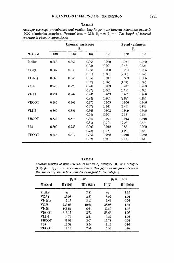
RESAMPLING INFERENCE IN REGRESSION 1291
TABLE 3
Average coverage probabilities and median lengths for nine interval estimation methods (3000 simulation samples). Nominal level = 0.95; f3) = 0; f3I = 4. The length of interval estimate is given in parentheses.
Unequal variances Equal variances 02 02
Method - 0.25 - 0.35 -0.5 - 1.0 - 0.25 - 1.0
Fieller 0.858 0.866 0.968 0.952 0.947 0.950 (0.98) (0.92) (2.48) (0.64)
VCJ(1) 0.887 0.848 0.961 0.950 0.904 0.935 (0.91) (0.89) (2.03) (0.62)
VHJ(1) 0.866 0.845 0.950 0.947 0.899 0.935 (0.87) (0.87) (1.94) (0.62)
VCJ8 0.946 0.920 0.968 0.953 0.947 0.939 (0.97) (0.90) (3.19) (0.63)
VHJ8 0.931 0.908 0.965 0.953 0.941 0.939 (0.93) (0.90) (2.69) (0.63)
VBOOT 0.886 0.902 0.973 0.955 0.956 0.946 (0.97) (0.91) (2.42) (0.64)
VLIN 0.865 0.891 0.969 0.952 0.949 0.948 (0.93) (0.90) (2.18) (0.64)
PBOOT 0.829 0.814 0.940 0.921 0.912 0.916 (0.84) (0.79) (2.05) (0.56)
PJ8 0.809 0.755 0.909 0.912 0.831 0.900 (0.78) (0.78) (1.90) (0.55)
TBOOT 0.755 0.816 0.960 0.948 0.918 0.949 (0.92) (0.90) (2.14) (0.64)
TABLE 4
Median lengths of nine interval estimates of category (II) and category (III). f30 = 0; f3I = 4; unequal variances. The figure in the parentheses is the number of simulation samples belonging to the category.
02 = -0.25 02 = - 0.35
Method II (199) III (2801) 11 (7) III (2993)
Fieller OC 3.81 oc 1.10 VCJ(1) 29.08 3.87 8.92 1.04 VHJ(1) 15.17 3.13 5.63 0.98 VCJ8 223.67 10.65 38.08 1.59 VHJ8 166.81 6.64 49.80 1.37 VBOOT 313.17 3.73 86.63 1.07 VLIN 14.75 2.91 5.82 1.02 PBOOT 55.05 3.07 17.78 0.93 PJ8 28.54 3.34 8.22 0.92 TBOOT 17.16 2.89 5.56 0.98

1292 C. F.J.WU
their intervals are quite big even in category (III) where Fieller's interval is reasonably tight but, of course, with poor coverage probability. In the other cases, the first seven methods all do reasonably well.
2. Effect of error variance heteroscedasticity. As the theory indicates, the performance is less desirable in the unequal variance case. Fieller's interval is far from being exact for /2 = - 0.25, - 0.35 and unequal variances. For equal variances Fieller's method is almost exact and the next six methods (t-inter- vals with various variance estimates) perform reasonably well even in the most nonlinear case /2 = - 0.25. The two retain-8 jackknife methods are least affected by the heteroscedasticity of variances.
3. Undercoverage of the percentile methods. This is very disappointing in view of the second-order asymptotic results on the bootstrap (Singh (1981); Beran (1982)) that are used as evidence of the superiority of the bootstrap approxi- mation over the classical t-approximation.
4. Fieller's nwthod is exact in the equal variance case even when the parameter is considerably nonlinear, but is vulnerable to error variance heteroscedastic- ity.
5. The linearization method is a winner. This is most surprising since we cannot find a theoretical justification. The intervals are consistently among the shortest, and the coverage probabilities are quite comparable to the others (except for f2 = -0.25, -0.35 and unequal variances where VCJ8 and VHJ8 are the best). The linearization method is compared favorably with Fieller's method. The former has consistently shorter intervals than the latter and the coverage probabilities are very close. For /2 = -0.25, -0.35 and unequal variances, VLIN has much shorter intervals and much higher coverage prob- abilities. Note that Fieller's intervals are unbounded in 199 (/,2 = -0.25) and 7( t2 = - 0.35) out of 3000 samples (Table 4).
6. Internal (curl) or external (hat) adjustment in jackknife variance estima- tion? In general the curl jackknife gives wider intervals than the hat jack- knife, but the coverage probabilities of the two methods are comparable. One possible explanation is that, if the /2 component of A - f in the definition of
s (4.4) is negative, it may push /2 closer to zero, resulting in a large value of as.
11. Concluding remarks and further questions. Al1hough the jackknife method has been around for a long time, the recent surge of interest in resampling inference is primarily due to Efron's (1979, 1982) contributions and his pursuasive arguments in favor of the bootstrap. In fact, there is no clear-cut choice between the two methods for bias reduction or variance estimation in the i.i.d. case. The main difference is in histogram-based interval estimation, where the delete-one jackknife is definitely inferior.
Our main contribution to the jackknife methodology is twofold: (i) emphasis on a more flexible choice of the subset size and (ii) proposal of a general weighting scheme for independent but nonexchangeable situations such as re- gression. Because of (i), interval estimators based on the jackknife histogram can be constructed. Standard results on the large sample behavior of the bootstrap

RESAMPLING INFERENCE IN REGRESSION 1293
histogram probably hold for the jackknife with a proper choice of subset size (see Wu (1985) for such results). Because of (ii), our proposed variance estimators are unbiased for homoscedastic errors and robust against heteroscedasticity. The weighting scheme is applicable to general independent situations. The scope of the jackknife methodology is substantially broadened.
Our analysis of the bootstrap gives a different picture from that of Efron (1982), which deals primarily with the i.i.d. problem. The bootstrap method seems to depend on the existence of an exchangeable component of a model. If such a component does not exist (e.g., heteroscedastic linear models, generalized linear models), it may result in serious problems such as bias and inconsistency as our examples show. It encounters similar difficulties in handling complex survey samples, where neither the independence nor the exchangeability assump- tion is satisfied (Rao and Wu (1985a)). We therefore advise against its indis- criminate use in complex situations. Important features of a problem should be taken into account in the choice of resampling methods. In fairness to the bootstrap, it is intuitively appealing, easy to program and works well when an exchangeable component exists and is bootstrapped. The last point is supported by the studies of Freedman and Peters (1984) and Carroll, Ruppert and Wu (1986). Bootstrap will undoubtedly remain a major tool in the resampling arsenal.
Several questions have been raised in the course of our study. We hope they will generate further interests and research in this area.
1. How can the subset size r in the weighted jackknife be determined? Choice of r appears to depend on computational consideration and purpose of analysis, e.g., interval estimation and bias-robustness of variance estimators.
2. The method for resampling residuals in Section 7 gives variance estimators that have better theoretical properties than the bootstrap. What resampling plans in (7.1) should be chosen? The choice depends on computational consid- eration and further theoretical aspects.
3. Is the weighted bootstrap variance estimator v* (6.12), in general, nearly unbiased as the encouraging simulation result may suggest?
4. The methods based on the bootstrap-histogram and the jackknife-histogram perform disappointingly in the simulation. Refinements of these methods are called for (e.g., Efron (1985); Loh (1987)). One obvious defect of the resample histogram is that they have shorter tails than their population counterparts. The handling of skewness may also be improper. Theoretical results that can explain small-sample behavior are needed.
5. A careful study of resampling methods for more complex problems such as those in Section 8 is needed. Are there any shortcuts for computing the weights (or approximate weights) and/or higher-order asymptotic properties? How can models with correlated errors be handled?
6. The factor (r - k + 1)/(n - r) in the weighted jackknife is used for scale adjustment. It can be applied either before or after the nonlinear transforma- tion (see (4.1) and (4.3)). What are the relative merits of the two scaling methods?

1294 C. F.J. WU
REFERENCES
ABRAMOVITCH, L. and SINGH, K. (1985). Edgeworth corrected pivotal statistics and the bootstrap. Ann. Statist. 13 116-132.
BERAN, R. (1982). Estimated sampling distributions: The bootstrap and competitors. Ann. Statist. 10 212-225.
CARROLL, R. J., RUPPERT, D. and Wu, C. F. J. (1986). Generalized least squares: Variance expansions, the bootstrap and the number of cycles. Unpublished.
DEMPSTER, A. P., LAIRD, N. M. and RUBIN, D. B. (1980). Iteratively reweighted least squares for linear regression when errors are normal/independent distributed. In Multivariate Analy- sis (P. R. Krishnaiah, ed.) 5 35-57. North-Holland, Amsterdam.
EFRON, B. (1979). Bootstrap methods: Another look at the jackknife. Ann. Statist. 7 1-26. EFRON, B. (1982). The Jackknife, the Bootstrap and Other Resampling Plans. SIAM, Philadelphia. EFRON, B. (1985). Bootstrap confidence intervals for a class of parametric problems. Biometrika 72
45-58. EFRON, B. and GONG, G. (1983). A leisurely look at the bootstrap, the jackknife and cross-validation.
Amer. Statist. 37 36-48. FAREBROTHER, R. W. (1985). Relations among subset estimators: A bibliographical note. Techno-
metrics 27 85-86. Fox, T., HINKLEY, D. and LARNTZ, K. (1980). Jackknifing in nonlinear regression. Technometrics 22
29-33. FREEDMAN, D. A. and PETERS, S. C. (1984). Bootstrapping a regression equation: Some empirical
results. J. Amer. Statist. Assoc. 79 97-106. FULLER, W. A. (1976). Introduction to Statistical Time Series. Wiley, New York. HEDAYAT, A. and WALLIS, W. D. (1978). Hadamard matrices and their applications. Ann. Statist. 6
1184-1238. HINKLEY, D. V. (1977). Jackknifing in unbalanced situations. Technometrics 19 285-292. HORN, S. D. and HORN, R. A. (1975). Comparison of estimators of heteroscedastic variances in linear
models. J. Amer. Statist. Assoc. 70 872-879. HORN, S. D., HORN, R. A. and DUNCAN, D. B. (1975). Estimating heteroscedastic variances in linear
models. J. Amer. Statist. Assoc. 70 380-385. HUBER, P. J. (1981). Robust Statistics. Wiley, New York. KISH, L. and FRANKEL, M. (1974). Inference from complex samples (with discussion). J. Roy.
Statist. Soc. Ser. B 36 1-37. LEHMANN, E. L. (1983). Theory of Point Estimation. Wiley, New York. LOH, W. Y. (1987). Calibrating confidence coefficients. J. Amer. Statist. Assoc. To appear. MCCARTHY, P. J. (1969). Pseudo-replication: Half-samples. Rev. Internat. Statist. Inst. 37 239-264. MCCULLAGH, P. (1983). Quasi-likelihood functions. Ann. Statist. 11 59-67. MCCULLAGH, P. and NELDER, J. A. (1983). Generalized Linear Models. Chapman and Hall, London. MILLER, R. G. (1974a). The jackknife-a review. Biometrika 61 1-15. MILLER, R. G. (1974b). An unbalanced jackknife. Ann. Statist. 2 880-891. NOBLE, B. (1969). Applied Linear Algebra. Prentice-Hall, New York. QUENOUILLE, M. (1956). Notes on bias in estimation. Biometrika 43 353-360. RAO, C. R. (1970). Estimation of heteroscedastic variances in linear models. J. Amer. Statist. Assoc.
65 161-172. RAO, J. N. K. (1973). On the estimation of heteroscedastic variances. Biometrics 29 11-24. RAO, J. N. K. and Wu, C. F. J. (1985a). Bootstrap inference for sample surveys. In Proc. 1984 ASA
Meeting, Section on Survey Research Methods 106-112. RAO, J. N. K. and Wu, C. F. J. (1985b). Inference from stratified samples: Second-order analysis of
three methods for nonlinear statistics. J. Amer. Statist. Assoc. 80 620-630. RUBIN, D. B. (1978). A representation for the regression coefficients in weighted least squares. ETS
Research Bulletin RB-78-1, Princeton, N.J. SHAO, J. and Wu, C. F. J. (1985). Robustness of jackknife variance estimators in linear models.
Technical Report No. 778, Univ. of Wisconsin-Madison. SINGH, K. (1981). On the asymptotic accuracy of Efron's bootstrap. Ann. Statist. 9 1187-1195.

RESAMPLING INFERENCE IN REGRESSION 1295
SUBRAHMANYAM, M. (1972). A property of simple least squares estimates. Sankhya Ser. B 34 355-356.
TUKEY, J. (1958). Bias and confidence in not quite large samples (abstract). Ann. Math. Statist. 29 614.
WEDDERBURN, R. W. M. (1974). Quasi-likelihood functions, generalized linear models and the Gauss-Newton method. Biometrika 61 439-447.
WILLIAMS, E. J. (1959). Regression Analysis. Wiley, New York. Wu, C. F. J. (1984). Jackknife and bootstrap inference in regression and a class of representations for
the LSE. Technical Report No. 2675, Mathematics Research Center, Univ. of Wisconsin-Madison.
Wu, C. F. J. (1985). Statistical methods based on data resampling. Special invited paper presented at IMS meeting in Stony Brook.
DEPARTMENT OF STATISTICS
UNIVERSITY OF WISCONSIN MADISON, WISCONSIN 53706
DISCUSSION
RUDOLF BERAN
University of California, Berkeley
My comments center on three topics: the resampling algorithm of Section 7 as a bootstrap algorithm; criteria for assessing performance of a confidence set; and robustifying jackknife or bootstrap estimates for variance and bias. It will be apparent that I do not accept several of Wu's conclusions, particularly those concerning the bootstrap. The implied criticism does not diminish the paper's merit in advancing jackknife theory for the heteroscedastic linear model.
1. The bootstrap idea is a statistical realization of the simulation concept: one fits a plausible probability model to the data and acts thereafter as though the fitted model were true. Suppose that the errors {ei} in the linear model (2. 1) are independent and that the c.d.f. of ei is F( /aj), where F has mean zero and variance one. Consistent estimates of the tail and of F are not available, in general. Nevertheless, let a ,i be an esimate of ai, such as ,n i = Iri(1 - 1/2
or air, = il(l - n-1k)-1/2, and let Fn be any c.d.f. with mean zero and variance one. The fitted model here is the heteroscedastic linear model parametrized by the estimates n3 {a,n i} and Fn. The appropriate bootstrap algorithm, which I will call the heteroscedastic bootstrap, draws samples from this fitted model.
Section 7 of the paper describes just this resampling procedure, without recognizing it as a bootstrap algorithm suitable for the heteroscedastic linear model. The two bootstrap algorithms that are discussed critically in Section 2 are not even intended for the heteroscedastic linear model. The first is designed for the homoscedastic linear model; the second for linear predictors based on multivariate i.i.d. samples (Freedman (1981)).
Let B,(1, {aI, F) and V,(f, {ai), F) be the bias and variance of g(f3n) under the heteroscedastic model described in the preceding paragraphs. The ap-