jacob a miller - connecting repositories · 2017. 12. 7. · numerical balancing in a humdi cation...
TRANSCRIPT

Numerical Balancing in a Humdification
Dehumidification Desalination System
by
Jacob A Miller
B.S., Yale University (2007)
Submitted to the Department of Mechanical Engineeringin partial fulfillment of the requirements for the degree of
Master of Science in Mechanical Engineering
at the
MASSACHUSETTS INSTITUTE OF TECHNOLOGY
September 2011
c© Massachusetts Institute of Technology 2011. All rights reserved.
Author . . . . . . . . . . . . . . . . . . . . . . . . . . . . . . . . . . . . . . . . . . . . . . . . . . . . . . . . . . . . . .Department of Mechanical Engineering
August 19, 2011
Certified by. . . . . . . . . . . . . . . . . . . . . . . . . . . . . . . . . . . . . . . . . . . . . . . . . . . . . . . . . .John H. Lienhard V
Collins Professor of Mechanical EngineeringThesis Supervisor
Accepted by . . . . . . . . . . . . . . . . . . . . . . . . . . . . . . . . . . . . . . . . . . . . . . . . . . . . . . . . .David E. Hardt
Chairman, Department Committee on Graduate Theses

2

Numerical Balancing in a Humdification Dehumidification
Desalination System
by
Jacob A Miller
Submitted to the Department of Mechanical Engineeringon August 19, 2011, in partial fulfillment of the
requirements for the degree ofMaster of Science in Mechanical Engineering
Abstract
This thesis details research on the thermal and concentration balancing of a humid-ification dehumidification desalination system. The system operates similarly to thenatural rain cycle. Seawater is heated, sprayed into an airstream to increase the air’shumidity, then pure water is condensed out of the same stream in a separate unit.These systems are typically inefficient due to entropy generation caused by mismatchbetween the temperature and humidity profiles in both the humidifier and dehumid-ifier components. Numerical models are developed for several different systems, andit is shown that for a given system with fixed inputs, entropy generation is minimizedby way of balancing; i.e., the extraction and reinjection of the water or air streamswithin the humidifier and dehumidifier to equalize the capacity rates of the streams.Several modifications to existing baseline cycles are made to reach cases of minimumentropy generation. In these cases, the performance of the system is dramaticallyimproved and the amount of energy needed to drive the system is reduced. For bothon and off-design models, the addition of multiple extractions markedly improves theperformance as compared to a baseline case with no extractions.
Thesis Supervisor: John H. Lienhard VTitle: Collins Professor of Mechanical Engineering
3

4

Acknowledgments
First and foremost, I would like to thank the entire Lienhard Lab for their knowl-
edge, support, and friendship. I learned so much in such a short period of time from
this community of brilliant students and faculty. I can only hope to encounter other
groups of this caliber as I continue my career.
I thank my advisor, John H. Lienhard V, for his invaluable guidance and for illu-
minating the importance of desalination research in the intersection of the fields of
energy, water, and sustainability. This project owes much to the quality of his advis-
ing.
As always, I am thankful for the love and encouragement from my family and friends
as I endeavored to produce a quality thesis on a strict time constraint.
Finally, I am pleased to thank GE Aviation for their funding and assistance while
completing this degree.
5

6

Contents
Abstract . . . . . . . . . . . . . . . . . . . . . . . . . . . . . . . . . . 3
Acknowledgments . . . . . . . . . . . . . . . . . . . . . . . . . . . . . 5
Table of Contents . . . . . . . . . . . . . . . . . . . . . . . . . . . . . 9
List of Figures . . . . . . . . . . . . . . . . . . . . . . . . . . . . . . . 13
List of Tables . . . . . . . . . . . . . . . . . . . . . . . . . . . . . . . 15
Nomenclature . . . . . . . . . . . . . . . . . . . . . . . . . . . . . . . 20
1 Introduction 21
1.1 Humidification Dehumidification Desalination Systems . . . . . . . . 22
1.1.1 Performance Metrics of HDH Systems . . . . . . . . . . . . . 24
1.2 A Review of Heat and Mass Exchangers . . . . . . . . . . . . . . . . 25
1.2.1 Heat Exchangers . . . . . . . . . . . . . . . . . . . . . . . . . 25
1.2.2 Heat and Mass Exchangers . . . . . . . . . . . . . . . . . . . . 27
1.3 Concept of Balancing . . . . . . . . . . . . . . . . . . . . . . . . . . . 30
1.3.1 Imbalanced HDH System . . . . . . . . . . . . . . . . . . . . . 30
1.3.2 Balanced HDH Systems . . . . . . . . . . . . . . . . . . . . . 33
1.4 Comparison to MED . . . . . . . . . . . . . . . . . . . . . . . . . . . 36
2 On-Design Humidification Dehumidification Model 39
2.1 Individual Humidifier and Dehumidifier . . . . . . . . . . . . . . . . . 40
2.2 Humidifier . . . . . . . . . . . . . . . . . . . . . . . . . . . . . . . . . 40
2.2.1 Governing Equations . . . . . . . . . . . . . . . . . . . . . . . 41
2.2.2 Results . . . . . . . . . . . . . . . . . . . . . . . . . . . . . . . 44
2.3 Dehumidifier . . . . . . . . . . . . . . . . . . . . . . . . . . . . . . . . 46
7

2.3.1 Governing Equations . . . . . . . . . . . . . . . . . . . . . . . 46
2.3.2 Results . . . . . . . . . . . . . . . . . . . . . . . . . . . . . . . 50
2.4 Combined System Model . . . . . . . . . . . . . . . . . . . . . . . . . 50
2.4.1 Zero Extraction Model . . . . . . . . . . . . . . . . . . . . . . 52
2.4.2 Single Extraction Model . . . . . . . . . . . . . . . . . . . . . 54
2.4.3 Dual Extraction Model . . . . . . . . . . . . . . . . . . . . . . 61
2.4.4 Multiple Extractions: Validating Multi-Extraction . . . . . . . 63
2.4.5 Validating On-Design Extraction Model . . . . . . . . . . . . 67
2.4.6 Impact of Effectiveness on Extraction . . . . . . . . . . . . . . 69
2.4.7 Avoiding Humidifier Temperature Crosses . . . . . . . . . . . 71
2.4.8 High GOR On-Design Cases . . . . . . . . . . . . . . . . . . . 73
2.5 Summary of On-Design HDH System . . . . . . . . . . . . . . . . . . 74
3 Off-Design Humidification Dehumidification Model 77
3.1 Finite Difference Humidifier Model . . . . . . . . . . . . . . . . . . . 78
3.1.1 Control Volume Analysis . . . . . . . . . . . . . . . . . . . . . 78
3.1.2 Determination of the Mass Transfer Coefficient . . . . . . . . 81
3.1.3 Solution of Humidifier Model . . . . . . . . . . . . . . . . . . 82
3.1.4 Humidifier Performance Evaluation . . . . . . . . . . . . . . . 84
3.1.5 Validation of Humidifier Model . . . . . . . . . . . . . . . . . 86
3.2 Finite Difference Dehumidifier Model . . . . . . . . . . . . . . . . . . 88
3.2.1 Control Volume Analysis . . . . . . . . . . . . . . . . . . . . . 89
3.2.2 Solution of Dehumidifier Model . . . . . . . . . . . . . . . . . 91
3.2.3 Dehumidifier Performance Evaluation . . . . . . . . . . . . . . 93
3.2.4 Dehumidifier Validation . . . . . . . . . . . . . . . . . . . . . 94
3.3 Full Cycle Model . . . . . . . . . . . . . . . . . . . . . . . . . . . . . 97
3.3.1 Water-Heated System Model . . . . . . . . . . . . . . . . . . . 98
3.3.2 Air-Heated System Model . . . . . . . . . . . . . . . . . . . . 101
3.4 Extractions in Off-Design Model . . . . . . . . . . . . . . . . . . . . . 102
8

4 Conclusions 107
4.1 On-Design Lessons Learned . . . . . . . . . . . . . . . . . . . . . . . 107
4.2 Off-Design Lessons Learned . . . . . . . . . . . . . . . . . . . . . . . 108
4.3 Future Work . . . . . . . . . . . . . . . . . . . . . . . . . . . . . . . . 109
4.4 Final Remarks . . . . . . . . . . . . . . . . . . . . . . . . . . . . . . . 110
A Comparison of Zero Extraction Cycles 111
Bibliography 118
9

10

List of Figures
1-1 Schematic diagram of an air heated HDH system . . . . . . . . . . . 23
1-2 Simple schematic of an air-heated CAOW HDH system . . . . . . . . 31
1-3 Unbalanced temperature profiles . . . . . . . . . . . . . . . . . . . . . 32
1-4 Unbalanced dehumidifier humidity profile . . . . . . . . . . . . . . . . 33
1-5 HDH dehumidifier with single water extraction point . . . . . . . . . 34
1-6 Fully balanced temperature profiles . . . . . . . . . . . . . . . . . . . 35
1-7 Balanced dehumidifier humidity profile . . . . . . . . . . . . . . . . . 35
1-8 Simple schematic of a MED cycle . . . . . . . . . . . . . . . . . . . . 37
1-9 Temperature and pressure per stage in an example MED plant . . . . 37
2-1 Two sub-component humidifier submodel . . . . . . . . . . . . . . . . 41
2-2 Total normalized entropy generation, humidifier submodel; εH = 0.8 . 45
2-3 Two sub-component dehumidifier submodel . . . . . . . . . . . . . . 47
2-4 Total normalized entropy generation, dehumidifier submodel; εD = 0.8 51
2-5 Air-heated CAOW HDH system without extraction . . . . . . . . . . 53
2-6 GOR vs. Mass Flow Rate Ratio for a 2 subcomponent, zero extraction
CAOW HDH Cycle . . . . . . . . . . . . . . . . . . . . . . . . . . . . 54
2-7 Air-heated CAOW HDH system with single water extraction . . . . . 56
2-8 Performance of a two subcomponent air heated cycle with water ex-
traction . . . . . . . . . . . . . . . . . . . . . . . . . . . . . . . . . . 57
2-9 Subcomponent HCR versus extraction rate for an air heated water
extraction cycle . . . . . . . . . . . . . . . . . . . . . . . . . . . . . . 58
2-10 Air-heated CAOW HDH system with single air extraction . . . . . . 59
11

2-11 Performance of a two subcomponent air heated cycle with air extraction 60
2-12 GOR vs. extraction rate for a two subcomponent water heated cycle
with water extraction . . . . . . . . . . . . . . . . . . . . . . . . . . . 61
2-13 GOR vs. extraction rate for a two subcomponent water heated cycle
with air extraction . . . . . . . . . . . . . . . . . . . . . . . . . . . . 61
2-14 Air-heated CAOW HDH system with dual air extraction . . . . . . . 62
2-15 Performance of a three subcomponent air heated cycle with air extraction 64
2-16 N Air Extractions . . . . . . . . . . . . . . . . . . . . . . . . . . . . 66
2-17 On-design validation of one versus two subcomponent models . . . . . 68
2-18 Impact of extraction on the two subcomponent HDH system model;
initially εD = εH = 0.8 . . . . . . . . . . . . . . . . . . . . . . . . . . 69
2-19 Performance of single extraction cycles at subcomponent effectiveness
εall = 0.9 . . . . . . . . . . . . . . . . . . . . . . . . . . . . . . . . . . 70
2-20 Temperature profiles of humidifiers for air-heated air extraction cycle
with GOR=7.2 . . . . . . . . . . . . . . . . . . . . . . . . . . . . . . 73
2-21 Temperature cross in humidifier for ε = 1 . . . . . . . . . . . . . . . . 75
3-1 Humidifier control volume analysis . . . . . . . . . . . . . . . . . . . 79
3-2 Linking of cells in the humidifier model . . . . . . . . . . . . . . . . . 83
3-3 Temperature and humidity profiles in the humidifier . . . . . . . . . . 85
3-4 Entropy production and effectiveness in the humidifier model . . . . . 86
3-5 Comparison of actual and calculated mass transfer coefficients . . . . 88
3-6 Control Volume of Counterflow Dehumidifier . . . . . . . . . . . . . . 89
3-7 Resistance network model for dehumidifier . . . . . . . . . . . . . . . 90
3-8 Linking of cells in the dehumidifier model . . . . . . . . . . . . . . . . 92
3-9 Temperature and humidity profiles in the dehumidifier . . . . . . . . 94
3-10 Entropy production and effectiveness in the dehumidifier model . . . 95
3-11 Peak GOR versus component size . . . . . . . . . . . . . . . . . . . . 100
3-12 Water production rate versus system size for various humidifier and
dehumidifer sizes . . . . . . . . . . . . . . . . . . . . . . . . . . . . . 101
12

3-13 Impact of water extraction on GOR and stream to stream variance . 104
A-1 Single component HDH Cycles . . . . . . . . . . . . . . . . . . . . . . 112
A-2 Zero extraction comparison for a 1, 2, and 3 subcomponent air heated
model . . . . . . . . . . . . . . . . . . . . . . . . . . . . . . . . . . . 114
13

14

List of Tables
2.1 Minimum entropy generation states from humidifier submodel . . . . 46
2.2 Minimum entropy generation states from dehumidifier submodel . . . 52
2.3 Zero extraction model input conditions for Figure 2-6 . . . . . . . . . 53
2.4 Subcomponent entropy production versus extraction rate for air heated
water extraction cycle . . . . . . . . . . . . . . . . . . . . . . . . . . 59
2.5 Two extraction model input conditions for Figure 2-15 . . . . . . . . 62
2.6 Input and output values for air-heated HDH cycle, εD = εH = 1 . . . 74
3.1 Humidifier model inputs . . . . . . . . . . . . . . . . . . . . . . . . . 84
3.2 Humidifier model validation . . . . . . . . . . . . . . . . . . . . . . . 87
3.3 Dehumidifier model inputs . . . . . . . . . . . . . . . . . . . . . . . . 93
3.4 Dehumidifier validation inputs - zero humidity case . . . . . . . . . . 96
3.5 Dehumidifier validation inputs - single exchanger case . . . . . . . . . 97
3.6 High GOR water-heated HDH cycle component data . . . . . . . . . 98
3.7 Comparison of high GOR water-heated HDH cycles . . . . . . . . . . 99
3.8 Comparison of two different air-heated HDH cycles . . . . . . . . . . 102
3.9 Impact of extraction on high GOR water-heated cycle . . . . . . . . . 103
15

16

Nomenclature
Acroynms
HDH Humidification Dehumidification
HME Heat and Mass Exchanger
ME Multi-extraction
MED Mutiple Effect Distillation
MSF Multi-Stage Flash
RO Reverse Osmosis
TTD Terminal Temperature Difference
Dimensionless Quantities
GOR Gained Output Ratio [mhfg/Q]
HCR Heat Capacity Rate ratio [Cc/Ch]
NTU Number of Transfer Units [UA/Cmin]
Pr Prandtl number [cpµ/k]
Re Reynolds number [ρvDh/µ]
RR Recovery Ratio [mpw/mw]
Sc Schmidt number [µ/ρ-DG]
Greek Symbols
α heat transfer coefficient [W/m2-K]
β mass transfer coefficient [kg/m2-s]
∆ change or difference [-]
ε effectiveness [-]
17

µ viscosity [kg/m-s]
ω humidity ratio [kg water vapor/kg dry air]
φ relative humidity [-]
ρ density [kg/m3]
Roman Symbols
z dimensionless component length [-]
H total enthalpy rate [kW]
m mass flow rate [kg/s]
Q heat transfer rate [kW]
Sgen entropy generation rate [kW/K]
A area [m2]
a specific surface area [m2/m3]
C heat capacity rate [kW/K]
cp specific heat capacity at constant pressure [kJ/kg-K]
Cf friction coefficient [-]
D diameter [m]
Dp nominal diameter of packing [m]
DG mass diffusivity in gas [m2/s]
Dh hydraulic diameter [m2]
G mass flux of gas stream [kg/m2-s]
h specific enthalpy [kJ/kg]
hfg specific enthalpy of vaporization [kJ/kg]
k thermal conductivity [W/m-K]
L mass flux of liquid stream [kg/m2-s]
m mass fraction [-]
mr mass flow rate ratio, mw/mda [-]
N number [-]
18

P absolute pressure [kPa]
s specific entropy [kJ/kg-K]
T temperature [◦C]
t thickness [m]
U overall heat transfer coefficient [W/m2-K]
V volume [m3]
V ar normalized variance [-]
z height [m]
Subscripts
a moist air
aw wall, air-side
c cold stream
d distillate
Di dehumidifier i
da dry air
dp dew point
ext extraction
G gas
h hot stream
Hi humidifier i
i inlet
inj injection
lm log mean
o oulet
pw product (pure) water
s surface
sat saturated condition
19

ss supersaturated
v vapor
w water
wb wet bulb
ww wall, water-side
int interface
max maximum
min minimum
Superscripts
a evaluated at bulk air temperature
ideal ideal condition
w evaluated at bulk water temperature
20

Chapter 1
Introduction
As the world population continues to expand and nations become wealthier and more
productive, demand for fresh water has grown. Residential, industrial, and agricul-
tural processes all consume vast quantities of water; with many of the world’s fresh
water resources already tapped, alternate solutions to acquiring this basic necessity
are under development. Desalination technology has existed for many years, from
the humble beginnings of small solar stills [1] to today’s colossal thermal desalination
plants in the Middle East and high-tech reverse osmosis plants all over the world.
Desalination is a broad term which refers to several technologies and processes that
remove salts from water, making it potable for human use. Any type of salt water can
be desalinated, from highly saline seawater to slightly brackish inland water, although
in general the greater the salt content, the more energy required to remove it. Desali-
nation is an energy intensive process and requires considerable capital expenditure,
making it far costlier than extracting fresh water from lakes, rivers, or groundwater.
Even so, use of desalination processes has skyrocketed over the last several decades
as water shortages in developing arid regions have driven demand for massive quanti-
ties of fresh water. The International Desalination Association (IDA) estimates that
there are now over 15,000 contracted desalination plants with a capacity of 71.7 billion
21

liters of drinkable water per day [2]. The online capacity is over 65.2 billion liters per
day, indicating that an additional 6.5 billion liters per day of future capacity is under
construction. The majority of plants in the Middle East employ large thermally pow-
ered processes such as multi-stage flash (MSF) and multi-effect distillation (MED)
plants. These plants are typically constructed alongside power plants to enable the
coproduction of electricity and water. The plants consume considerable amounts of
natural gas or oil to create steam which is used to generate electricity and drive the
water/salt separation process. In locations such as the United States, where fossil
fuels and construction of large plants are costlier, smaller, electrically driven reverse
osmosis (RO) desalination plants have been the systems of choice. However, there are
a variety of markets where neither of these technologies fully meets the needs of the
customer. Many new technologies are emerging from universities and corporations
to meet customers’ demands for lower cost, less energy intensive, easier to use tech-
nologies. Humidification dehumidification (HDH) desalination is one such potential
technology and it is the focus of this study.
1.1 Humidification Dehumidification Desalination
Systems
Humidification dehumidification systems have been employed for small scale desalina-
tion processes when large scale thermal systems such MSF and MED are unsuitable
for the application due to cost and size, or where there is unsuitable electrical infras-
tructure to run RO. The HDH technology is a natural evolution from the solar still
[3], and to date most systems have had a similar or slightly higher effectiveness of
water production [4]. This, in turn, means water produced by HDH has often proved
expensive [5, 6] due to the low efficiency of the separation pricess. Renewed efforts
to increase this effectiveness are ongoing [7, 8, 9, 10], and this work also analyzes a
22

method to improve the efficiency of such devices. The thermodynamic cycle utilized
in HDH technology is analogous to the natural rain cycle; just as in nature, water
vapor is created by the evaporation of liquid water and then recondensed. Therefore,
there are two major components of the HDH system: the humidifier and dehumidifier.
In this research, a direct contact counterflow humidifier is employed to humidify the
carrier gas stream. Next, an indirect contact counterflow dehumidifier recondenses
liquid water out of the humid air. In between the two components a third component,
a heater which may heat either the air or water stream, is added to drive the process.
Figure 1-1 [11] illustrates a representative HDH system configuration.
DehumidifierHumidifier
FreshWaterExit
SeawaterInlet
Heat Source
Brine Exit
Figure 1-1: Schematic diagram of an air heated HDH system
The process involves the separation of pure water from a liquid mixture, typically
23

sea or brackish water. A humidifier is employed to evaporate water into a carrier
gas. Any salt water not evaporated is rejected as brine. The moisture content of the
carrier gas is increased, and it is then passed to a dehumidifier. In the dehumidifier,
water is condensed out of the moist carrier gas and removed from the system. Heat
or work must be input between or within any of the components in the air or water
loop to drive the cycle. In summary, salt water and heat are input into the system
(as well as some small amount of electric work to power any fans and pumps, if used)
while the outputs are pure water and concentrated salt brine.
1.1.1 Performance Metrics of HDH Systems
The following parameters are typically used to describe the performance of an HDH
system.
The figure of merit that defines energy performance for HDH and other thermal
desalination systems is called the Gained Output Ratio (GOR). This parameter is
a dimensionless number that measures the effectiveness of water production and is
directly related to the amount of heat recovered within the system. Thus, a higher
GOR corresponds to a more efficient system.
GOR =mpwhfg
Qin
(1.1)
where mpw is the flow rate of the product water stream, hfg is the latent heat of
evaporation of the water, and Qin is the energy input into the system. This figure of
merit compares the amount of energy required to run the cycle with the amount of
energy required to vaporize the product water.
Another frequently measured metric is the recovery ratio (RR). The recovery ratio
is the fraction of product water to saline water input into the system:
24

RR =mpw
mw,i
(1.2)
A high recovery ratio is also desirable as more water is recovered from the inlet stream,
requiring a smaller flow (thus, a smaller pump) of inlet water.
1.2 A Review of Heat and Mass Exchangers
The HDH system consists of two main components: a humidifier and a dehumidifier.
These components are both heat and mass exchangers (HMEs), as within both com-
ponents heat is transferred between the air and water streams in order to warm or
cool the flow, and mass is transferred by way of water vapor diffusing in or out of the
air stream. In order to describe key operating paramaters of these systems, terminol-
ogy must be developed to describe a few key phenomena. Section 1.2.1 formulates
terminology for heat exchangers while Section 1.2.2 extends these concepts to heat
and mass exchangers.
1.2.1 Heat Exchangers
While the humidifier and dehumidifier utilized in HDH systems are heat and mass ex-
changers, it is useful to review the concepts behind a simple heat exchanger as many
of the definitions used in this research are derived from heat exchanger concepts. Sev-
eral methods are available to analyze a heat exchanger, but one commonly employed
method in two-stream counterflow design is the effectiveness method [12, 13]. This
approach is often used when the inlet or outlet temperatures must be calculated for
given mass flow rates and exchanger design. In the effectiveness method, exchanger
effectiveness may be characterized as the ratio of heat transferred to the ideal amount
of heat transfer which could take place in an infinitely long exchanger. The actual
amount of heat transferred between the two streams of the exchanger, assuming fixed
25

specific heats, is given by the first law of thermodynamics
Q = Ch(Th,in − Th,out) = Cc(Tc,in − Tc,out) (1.3)
where Ch = (mcp)h and Cc = (mcp)c are the capacity rates of the hot and cold streams
respectively.
The temperature difference between the two streams acts as a driving force to
propel heat from one stream to another. Any heat lost by one stream is picked up
by the other. It is assumed that in an ideal heat exchanger, the ideal amount of heat
may be transferred when one stream gives up all available heat to the opposed stream.
Thus, the system must be limited by the stream with the lowest thermal capacity rate,
Cmin. This stream, when all available heat is exchanged, changes temperature from
the inlet temperature of one stream to that of the other. Therefore, the maximum
amount of heat transferred is given by
Qmax = Cmin(Th,in − Tc,in) (1.4)
where Cmin is the capacity rate of the stream with the smallest thermal capacity.
Effectiveness, ε, then may be described as
ε =Q
Qmax
(1.5)
where the value of Q may be found from either the cold stream or hot stream, as
both are equal. The value of effectiveness is a useful way to describe the performance
of a heat exchanger. For a given effectiveness, mass flow rates, inlet hot stream
temperature, and inlet cold stream temperature, the outlet conditions may be found
via Equations 1.3, 1.4 and 1.5.
In order to optimize the performance of a heat exchanger, irreversibilities must
be minimized. If entropy generation due to irreversibilities is minimized within the
26

component, a higher component efficiency may be realized. From the control volume
form of the second law as applied to the heat exchanger, entropy generation may be
calculated in terms of the inlet and outlet states
Sgen = mc(sout − sin)c + mh(sout − sin)h
= mccp,c ln
(Tc,outTc,in
)+ mhcp,h ln
(Th,outTh,in
). (1.6)
It may be found that Sgen is minimized when the heat capacity rates are equal [14].
Thus, one further definition is useful in this analysis: the heat capacity rate ratio is
defined as [15]
HCR =Cc
Ch
=(mcp)c(mcp)h
. (1.7)
For any value of effectiveness and for fixed inlet temperatures, when HCR is equal
to unity, the non-dimensionalized entropy generation reaches a minimum [14, 16].
Consequently, this condition is said to be “balanced”. The term balanced implies
that the system is thermally equalized and the change in temperature of the hot
stream is equal to that of the cold. Both streams have a linear temperature variation
with equal slope such that the ∆T between the two is constant. As the capacity
rates change and HCR strays further from 1, entropy generation increases and the
performance of the heat exchanger suffers. Previously attainable outlet temperatures
are no longer realistic because the capacity rates have changed. Thus, a balanced
heat exchanger optimizes the performance of the system.
1.2.2 Heat and Mass Exchangers
In a heat and mass exchanger, such as either the humidifier or dehumidifier in an
HDH desalination cycle, mass is exchanged via evaporation or condensation of water,
27

respectively. Whereas the heat exchanger transfers heat by a temperature gradient
between the two streams, the driving force of a heat and mass exchanger is both
the temperature gradient and the concentration gradient. In the HDH system, the
concentration of water vapor in the air stream drives the mass transfer between the
liquid and gaseous streams. It is useful to characterize a heat and mass exchanger in
similar terms to the heat exchanger, but some modifications must be applied to the
equations introduced in Section 1.2.1 to account for mass transfer. While Equation 1.5
defines effectiveness as the ratio of heat transfer to ideal heat transfer, the analogous
equation in a heat and mass exchanger is the ratio of the actual change in total
enthalpy rate of either stream to the maximum (or ideal) change in total enthalpy
rate. Therefore, effectiveness is given as
ε =∆H
∆Hmax
(1.8)
where ∆H = mw,ihw,i − mw,ohw,o for the water stream or ∆H = mda,iha,i − mda,oha,o
for the air stream. Additionally, ∆Hmax = mw,ihw,i − (mw,ohw,o)ideal or ∆Hmax =
mda,iha,i − (mda,oha,o)ideal for the water and air streams respectively.
The ideal values of enthalpy, hidealw,o and hideala,o , are the values of enthalpy of water at
the air inlet temperature and saturated air at the inlet water temperature respectively
(where P is taken at the actual pressure conditions of the stream).
The change of terms from Q to H is driven by the necessity to include the humidity
of the air in the amount of energy transferred. Neglecting pressure variation, the
enthalpy of moist air is a function of temperature, pressure, and humidity ratio, such
that
dha = cp,adT +
(∂ha∂ω
)∣∣∣∣P,T
dω. (1.9)
It is clear that in the case of the heat exchanger, dha reduces to cp,adT because dω = 0.
28
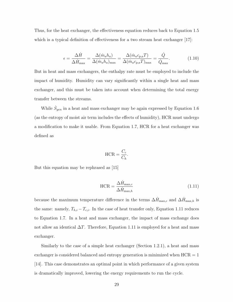
Thus, for the heat exchanger, the effectiveness equation reduces back to Equation 1.5
which is a typical definition of effectiveness for a two stream heat exchanger [17]:
ε =∆H
∆Hmax
=∆(maha)
∆(maha)max
=∆(macp,aT )
∆(macp,aT )max
=Q
Qmax
. (1.10)
But in heat and mass exchangers, the enthalpy rate must be employed to include the
impact of humidity. Humidity can vary significantly within a single heat and mass
exchanger, and this must be taken into account when determining the total energy
transfer between the streams.
While Sgen in a heat and mass exchanger may be again expressed by Equation 1.6
(as the entropy of moist air term includes the effects of humidity), HCR must undergo
a modification to make it usable. From Equation 1.7, HCR for a heat exchanger was
defined as
HCR =Cc
Ch
.
But this equation may be rephrased as [15]
HCR =∆Hmax,c
∆Hmax,h
(1.11)
because the maximum temperature difference in the terms ∆Hmax,c and ∆Hmax,h is
the same: namely, Th,i −Tc,i. In the case of heat transfer only, Equation 1.11 reduces
to Equation 1.7. In a heat and mass exchanger, the impact of mass exchange does
not allow an identical ∆T . Therefore, Equation 1.11 is employed for a heat and mass
exchanger.
Similarly to the case of a simple heat exchanger (Section 1.2.1), a heat and mass
exchanger is considered balanced and entropy generation is minimized when HCR = 1
[14]. This case demonstrates an optimal point in which performance of a given system
is dramatically improved, lowering the energy requirements to run the cycle.
29

1.3 Concept of Balancing
As noted in Section 1.2.1, a heat exchanger is thermally balanced when the heat
capacity ratio, HCR, is equal to one. While this is a well known concept for heat
exchangers, it has been recently applied to heat and mass exchangers [14] as well. To
completely balance a heat and mass exchanger, the driving force of energy transfer,
namely a combination of temperature and mass concentration difference, must be
balanced. A balanced HDH system maintains a constant driving force by maintaining
a constant difference in temperature and mass concentration between the air and
water streams of both the humidifier and the dehumidifier. In the case of HDH
desalination, the mass concentration difference is a function of the humidity of the
bulk air stream and of the interfacial region between air and water.
In order to balance the humidifier and dehumidifier, the air and water streams of
each must transfer heat between the two while the driving force within the system
is kept constant. In such a case, the temperature and mass concentration profiles
of the two streams along the length of the humidifier and dehumidifier are parallel.
In an unbalanced case, the heat flow from one stream to the other is far from ideal
because the heat capacity of one stream is dissimilar to the other. If one stream is
unable to transfer enough heat to the other, the temperature gap between the streams
widens and the system becomes less efficient. Conversely, when the heat capacity rate
between the streams is equivalent, the heat flow between the streams is optimized,
temperature and concentration divergences are eliminated, and efficiency increases.
In the following sections, a simple analysis of an unbalanced and a balanced HDH
system is presented.
1.3.1 Imbalanced HDH System
A schematic diagram of a simple HDH desalination system is presented in Figure 1-2.
An unoptimized system consists of three components: the humidifier, dehumidifier,
30

and a heater. The system in Figure 1-2 is an air heated, closed air open water system
(CAOW), though there are many permutations of such systems [7]. Cool seawater
enters at the bottom of the dehumidifier and is heated by the warm air entering at the
top in a counterflow configuration. As the air cools, pure water condenses out of the
stream and exits the component. The heated water enters the top of the humidifier
which warms and humidifies the incoming air from the bottom of the device. The
water cools, and any water that is not evaporated exits the component as brine. The
warm air is further heated in the heater between the air outlet of the humidifier and
inlet of the dehumidifier.
Figure 1-2: Simple schematic of an air-heated CAOW HDH system
A system such as the one displayed in Figure 1-2 may be optimized for components
of given effectiveness by varying such parameters as the inlet temperatures and mass
flow rates. However, it is not possible to balance both the humidifier and dehumidifier
31

(a) Dehumidifier temperature profile (b) Humidifier temperature profile
Figure 1-3: Unbalanced temperature profiles
simultaneously in this configuration. A single component may be balanced such that
HCR = 1, but this will typically leave the other component unbalanced. Figures 1-3a
and 1-3b illustrate the temperature profiles of an example case where the components
are unbalanced. As water enters the dehumidifier at 30◦C, it is gradually heated by
the air. The temperature profiles are not parallel because the capacity rates of the
streams are not matched. Therefore, water is not sufficiently heated in 1-3a and
exits the component a relatively low temperature of 50◦C. Similarly, the profiles are
not matched in the humidifier shown in 1-3b. Additionally, due to the low inlet
water temperature, the air in the humidifier does not reach a high temperature at
the oulet. This result lowers performance for two reasons: first, even if the outlet
air is saturated, the absolute humidity in the air is relatively low compared to a case
where the air leaves at a much higher temperature. This results in less vapor entering
the dehumidifier so less product water can be expected. Second, much more energy
much be added to the system by way of the heater to raise the temperature of the air
before it enters the system. As the performance metric, GOR, is a function of both
the flow rate of product water as well as the input heat, this imbalance directly (and
negatively) impacts the value of GOR.
As discussed in Section 1.2.2, the humidifier and dehumidifer in an HDH cycle
32

are heat and mass exchangers. Therefore, unlike a heat exchanger, it is not only the
temperature profiles that need to be balanced, but the concentration profiles as well.
Figure 1-4 illustrates the corresponding humidity profile derived from Figure 1-3a.
It is clear that at the component is very unbalanced as the profiles are not parallel,
particularly at the hotter end of the equipment where they diverge considerably.
Figure 1-4: Unbalanced dehumidifier humidity profile
1.3.2 Balanced HDH Systems
It has been proposed that to balance the humidifier and dehumidifier fluid from either
the air or water stream may be extracted from one one component and injected into
the other [14, 18]. An extraction may be placed at any height along the length of
the component and does not necessarily need to be injected at the same height, or
temperature (though injecting at the same temperature is favorable as it circumvents
mixing losses), in the other. By changing the heat capacity rate of the streams at any
point inside the component, the temperature and concentration gradients of the two
streams may be adjusted, forcing their profiles closer to each other in order to reduce
entropy generation at a given height within the component. For example, extracting
water from the dehumidifier per Figure 1-5a will adjust the temperature profile of
the water stream and bring it closer to a parallel arrangement with the air stream
33

temperature profile. Additionally, the extraction adjusts the concentration profiles,
though as seen in Figure 1-5b, the impact here is smaller. Nonetheless, this single
extraction point reduces the entropy generation in the component. If this combination
of extraction and injection is performed multiple times, in an arrangement known as
multi-extraction (ME), the difference between the two streams in both components
is reduced along the entire length of the device as seen in Figures 1-6a and 1-6b.
(a) Dehumidifier temperature profile (b) Dehumidifier humidity profile
Figure 1-5: HDH dehumidifier with single water extraction point
In the fully balanced system, the maximum water temperature (before heating)
has been increased from 50 to 85◦C by reducing the terminal temperature difference in
the dehumidifier [19]. It is possible to increase the temperature range with a single or
small number of extraction points, and such balancing would improve GOR. However,
this method will not have a value of GOR which matches an equivalent MED system
because there is a finite stream to stream temperature difference to drive the rate
processes. With a single extraction, the slope of the temperature profile within a
component can be improved to better match the adjacent stream, but there will still
be a large divergence of the two streams away from the system inlet, outlet, and
extraction point. Only when there are multiple extractions can the stream profiles
be forced together along the entire length of the component causing the mismatch
between the streams to reach a minimum. In this fully balanced case, the system
34

(a) Dehumidifier temperature profile (b) Humidifier temperature profile
Figure 1-6: Fully balanced temperature profiles
has a similar temperature range to a comparable MED system and, importantly, has
reduced entropy generation due to small and constant mismatch between the profiles
of each stream.
Figure 1-7: Balanced dehumidifier humidity profile
Additionally, the concentration profiles are considerably more parallel in the fully
balanced case. Per Figure 1-7, the interface humidity closely matches the humidity in
the bulk airflow. However, it is important to note that even though the temperature
profile is fully balanced, the concentration profile is not: there is still variance in
the profile, particularly at high temperatures. This result comes from the nonlinear
relationship between temperature and humidity. As temperature increases, humidity
35

increases exponentially. In fact, Thiel et. al [20] show that while the ideal case is
one where the variance in both driving forces is equal to zero, it is not possible to
achieve this state. If one driving force variance is brought to zero, the other will
have a finite, non-zero value. Thus, in Chapters 2 and 3, when cycles are created
to minimize entropy generation via extraction, the variance does not become zero in
both driving forces.
1.4 Comparison to MED
In this section, HDH technology will be put side by side with a Multiple Effect
Distillation (MED) system. A useful comparison of thermal performance is drawn in
order to illustrate the aims of thermal balancing delineated in Section 1.3.
MED consists of several consecutive chambers (effects) in which seawater is va-
porized and subsequently cooled to form pure liquid water per Figure 1-8. In a single
effect system, the input heat required to vaporize the water is equivalent to the latent
heat of evaporation, hfg, for the mass of water transformed from a liquid to gaseous
state. All of the heat input into the system is used once to evaporate the water and
there is no heat recovery. This cycle corresponds to a Gained Output Ratio (GOR)
of about 1. 1
To improve GOR, heat can be recycled from this first effect to evaporate an
additional mass of water in subsequent effects. In a typical arrangement like Figure
1-8, no additional heat supplements the downstream effects, and the heat from the
previous effect is recovered in the condenser to power the boiler of the next effect.
Thus, each effect will be at a lower temperature than the preceding, and therefore
the pressure must be reduced at each stage in order to induce vaporization. Ideally,
this process could be repeated in an infinite number of effects, but in application the
1Recall per Section 1.1.1, GOR is the figure of merit that describes HDH as well as other thermaldesalination systems and will be utilized throughout this paper to evaluate the performance ofvarious system configurations.
36

CB
CB
CB
CB
B
C
�in
Decreasing temperature, pressure
Vapor
Condensate
Brine
Figure 1-8: Simple schematic of a MED cycle
number of effects is limited by the boiling point elevation of evaporating seawater,
thermal losses, and the size of the equipment; therefore, there is a finite temperature
drop from each stage to the next. If the system is sized to produce an equivalent mass
of water in each stage, the GOR is approximately equal to the number of stages. For
instance, for the system mapped in Figure 1-9, ideally the GOR is about 13.
P [b
ar]
T sa
t[°
C]
90
30
0.9
0.0
40
N[# of stages]
1 2 3 4 5 6 7 8 9 10 11 12 13
Figure 1-9: Temperature and pressure per stage in an example MED plant
For a comparable HDH system (Figure 1-2), the cycle is not broken up into sep-
arate effects because the evaporation and condensation do not occur at a constant
37
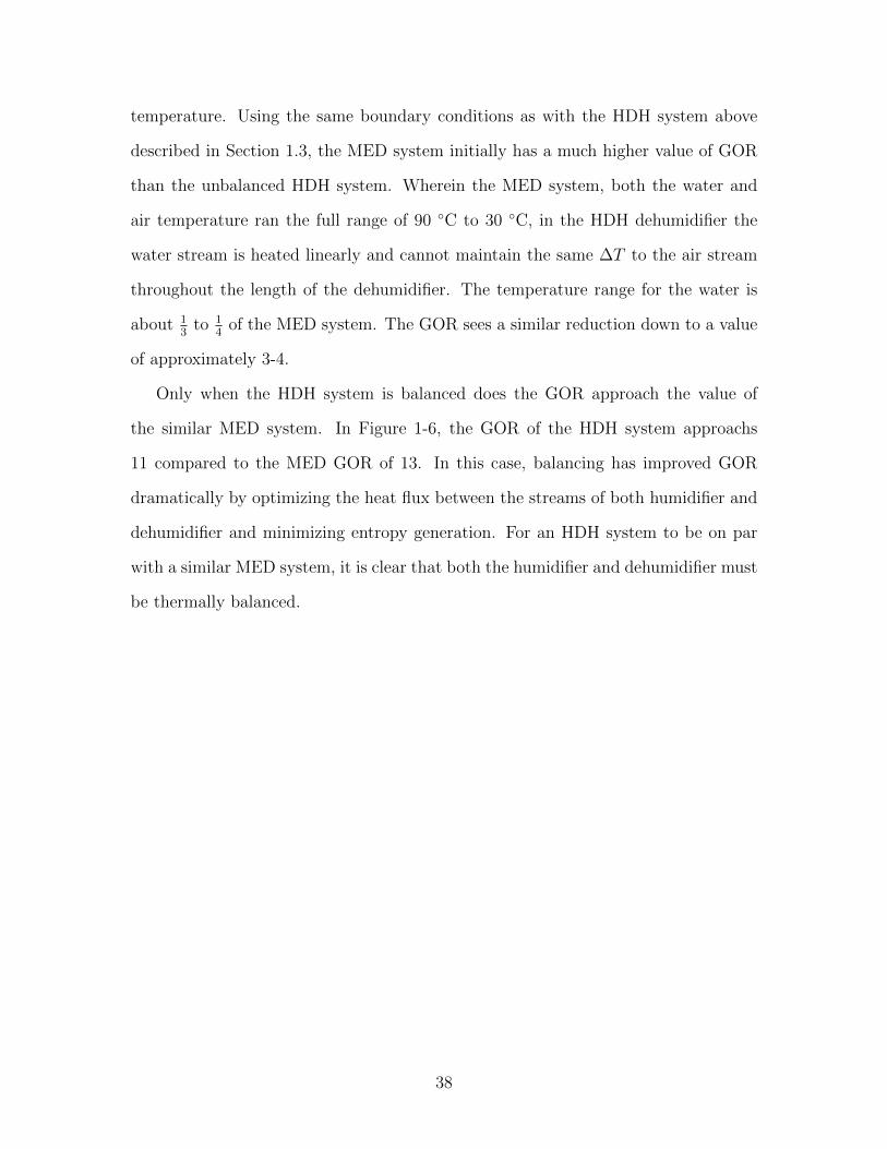
temperature. Using the same boundary conditions as with the HDH system above
described in Section 1.3, the MED system initially has a much higher value of GOR
than the unbalanced HDH system. Wherein the MED system, both the water and
air temperature ran the full range of 90 ◦C to 30 ◦C, in the HDH dehumidifier the
water stream is heated linearly and cannot maintain the same ∆T to the air stream
throughout the length of the dehumidifier. The temperature range for the water is
about 13
to 14
of the MED system. The GOR sees a similar reduction down to a value
of approximately 3-4.
Only when the HDH system is balanced does the GOR approach the value of
the similar MED system. In Figure 1-6, the GOR of the HDH system approachs
11 compared to the MED GOR of 13. In this case, balancing has improved GOR
dramatically by optimizing the heat flux between the streams of both humidifier and
dehumidifier and minimizing entropy generation. For an HDH system to be on par
with a similar MED system, it is clear that both the humidifier and dehumidifier must
be thermally balanced.
38

Chapter 2
On-Design Humidification
Dehumidification Model
In order to evaluate the impact of multi-extraction (ME) on the HDH system, two
thermodynamic cycle models have been created. These models are considered to be
on-design: they are “black-box” models that do not evaluate transport properties.
They are evaluated thermodynamically for feasability. In Chapter 3, off-design mod-
els are explored which simulate real systems utilizing transport properties. In this
chapter, first, a model that treats the humidifier and dehumidifier as distinct and
separate units was designed to evaluate the impact of ME on each component’s total
entropy production. Minimizing entropy production in each unit should in turn in-
crease total system performance when the humidifier and dehumidifier are considered
in relation to the total desalination cycle. In Section 2.4, the two separate units are
tied together with the addition of the heater to produce the complete cycle. In this
case, the entire system is included in the model and the thermal performance, in
terms of GOR, may be determined.
39

2.1 Individual Humidifier and Dehumidifier
Before creating a full system cycle, the humidifier and dehumidifier are analyzed as
individual units. While system parameters such as GOR and RR cannot be deter-
mined in this initial model (as there is no full system to evaluate), from Narayan
et al. [14] it is clear that entropy generation within the component directly impacts
performance. In this study, entropy generation will be evaluated for individual com-
ponents undergoing a single extraction or injection. The following assumptions are
made for these models:
• The cycle operates under steady state conditions.
• Pumping and blowing power is negligble.
• There are no pressure losses.
• All components are adiabatic with respect to their surroundings, i.e., heat lossis negligible.
• Kinetic and potential energy terms are not included in the energy balance.
2.2 Humidifier
In the first pass, the humidifier is “split” into two separate subcomponents per Figure
2-1. This method allows for a single extraction or injection stream to be inserted
between the two subcomponents. Each subcomponent may be analyzed individually,
or the entire humidifier may be scrutinized. With the water and air inlet states
specified (temperature, mass flow rate, humidity in the air stream) as well as the
extraction rate and the total component effectiveness, the only unknowns in the
system are the outlet temperatures and outlet mass flow rate of water (dry air mass
flow rate is assumed to be constant). These three unknowns are solved via three
equations: a first law energy balance, a mass balance on water, and the effectiveness
equation. Additionally, another first law control volume is drawn around the injection
40

site to determine the state of water entering humidifier 2. Finally, the second law is
used as a check to ensure no components are in violation of entropy production.
Figure 2-1: Two sub-component humidifier submodel
2.2.1 Governing Equations
The following are governing equations for the humidifier. Shown below are equations
for the entire humidifier (both components and injection). The same equations are
utilized for the individual subcomponents as well, with the appropriate inlet and out-
let states for each.
41

Mass Balance
The dry mass flow of air is constant through the humidifier, thus each state has an
identical mass flow rate (in kg-dry air/s). The mass flow rate of water (in kg/s) en-
tering the system is a fixed, known value, but the subsequent states are not identical
to the first. Water evaporates as it passes through each humidifier stage, reducing the
flow rate downstream. This loss of water is taken into account in Equations 2.2 and
2.4 by the mωa terms where ω is the humidity ratio of the air stream, in kg-water/kg-
dry air. Additionally, per Equation 2.3, the injection point adds (or removes) extra
water into the stream.
mda,H2,i = mda,H2,o = mda,H1,i = mda,H1,o (2.1)
mw,H1,o = mw,H1,i − (mda,H1,oωa,H1,o − mda,H1,iωa,H1,i) (2.2)
mw,H2,i = mw,H1,o + mw,inj (2.3)
mw,H2,o = mw,H2,i − (mda,H2,oωa,H2,o − mda,H2,iωa,H2,i) (2.4)
First Law Energy Balance
A control volume is drawn around the full system (both components). Energy enters
the system at the air and water inlets as well as the injection site. Energy exits the
control volume at the air and water oulets. Thermophysical pure water properties 1,
such as enthalpy, hw, come from the property correlation of Harr, Gallagher and Kell
[22]. Thermophysical properties of moist air are derived from Hyland and Wexler [23]
(similar to ASHRAE’s in [24]) and treat humid air as a binary mixture of dry air and
1All water streams in this paper are considered to be pure water for ease of calculation. Sea-water properties such as enthalpy and entropy vary by under 10% from that of pure water for thetemperature ranges evaluated in this paper [21].
42

water vapor. Specifically, ha = hda + ωhv.
0 = mw,H1,ihw,H1,i − mw,H2,ohw,H2,o + mda,H2,iha,H2,i − mda,H1,oha,H1,o + mw,injhw,inj
(2.5)
A separate control volume is drawn around the injection site in order to correctly
assess the temperature of the water immediately downstream of the injection.
mw,H1,ohw,H1,o + mw,injhw,inj = mw,H2,ihw,H2,i (Injection site) (2.6)
Second Law
The second law is calculated for the same control volume as in the first law. The
entropy generation in the humidifier, Sgen,H , is evaluated to ensure it is greater than
zero and the second law has not been violated for a given set of input conditions.
Entropy values, s, are again derived from Harr, Gallagher and Kell [22] and Hyland
and Wexler [23]. Like with enthalpy, entropy for moist air is described as a mixture
of dry air and water vapor: sa = sda + ωsv.
Sgen,H = mw,H2,osw,H2,o− mw,H1,isw,H1,i + mda,H1,osa,H1,o− mda,H2,isa,H2,i− mw,insw,inj
(2.7)
Effectiveness
Per Section 1.2.2, the effectiveness is the final equation to solve the unknown outlet
states of the system. Effectiveness compares the actual versus ideal energy transfer
for each stream. The ideal values of enthalpy, hidealw,H,o and hideala,H,o, are the values of
enthalpy of water at the air inlet temperature and saturated air at the inlet water
temperature respectively. The total humidifier effectiveness, εH , is defined as the
43

maximum of the effectiveness of the air and water streams.
Qw,H = mw,H,ihw,H,i − mw,H,ohw,H,o + mw,injhw,inj (2.8)
Qidealw,H = mw,H,ihw,H,i − mw,H,oh
idealw,H,o + mw,injhw,inj (2.9)
Qa,H = mda,H,iha,H,i − mda,H,oha,H,o (2.10)
Qideala,H = mda,H,iha,H,i − mda,H,oh
ideala,H,o (2.11)
εw,H =Qw,H
Qidealw,H
(2.12)
εda,H =Qa,H
Qideala,H
(2.13)
εH = max(εw,H , εa,H) (2.14)
2.2.2 Results
A comprehensive study was previously performed which demonstrated that the non-
dimensional entropy production is minimized and that a heat and mass exchanger
reaches a balanced state when HCR = 1 for a component of fixed energy effectiveness
[15]. In the case of analyzing the individual humidifier and dehumidifier, it was found
that this statement holds true for cases when an extraction or an injection is applied
to the component. At this state, heat flow between the air and water stream is op-
timized and entropy reaches a minimum for the given boundary conditions. With
no extraction, a certain mass flow rate ratio will balance each component separately
minimizing the entropy generation for either the humidifier or dehumidifier. How-
ever, these components do not exhibit optimized temperature profiles thus entropy
generation may be reduced by an appropriate extraction or injection.
Figure 2-2 illustrates the impact of extracting or injecting into the water stream
when total effectiveness is held at εH = 0.8. The curves are generated by varying the
mass flow rate ratio while keeping all other inputs constant. It is clear that, as within
44

the non-extraction cases, when flow is injected the normalized entropy generation is
still minimized in the balanced condition, i.e. HCR = 1. Additionally, it may be seen
that the Sgen vs. HCR curve shifts for a given injection or extraction rate such that
the normalized entropy generation may be altered. In this case, injecting flow reduces
the total normalized entropy generation at its minimum point and along the curve.
The following Table 2.1 illustrates the results from the run with the smallest entropy
generation in Figure 2-2 (namely, 60% injection rate at HCR = 1). The specified
input values (boundary conditions) are in bold while the resultant values are in plain
text.
Figure 2-2: Total normalized entropy generation, humidifier submodel; εH = 0.8
45

State Mass Flow Temperature Relative Humidity[kg/s] [◦C] [-]
W,H1,i 1.00 55.0 –W,H1,o 0.979 41.2 –INJ 0.600 46.8 –W,H2,i 1.579 43.3 –W,H2,o 1.568 38.6 –DA,H1,o 0.524 52.3 1.0DA,H1,i 0.524 42.8 1.0DA,H2,o 0.524 42.8 1.0DA,H2,i 0.524 35.0 1.0
Table 2.1: Minimum entropy generation states from humidifier submodel
2.3 Dehumidifier
Like the humidifier, the dehumidifier is “split” into two separate subcomponents per
Figure 2-3. Again, the water and air inlet states are specified (temperature, mass flow
rate, humidity in the air stream) as well as the extraction rate, the only unknowns
in the system are the outlet temperatures and outlet mass flow rate of product water
(dry air mass flow and inlet water flow rates are assumed to be constant). These
three unknowns are solved via three equations: a first law energy balance, a mass
balance, and the effectiveness equation. The second law is used as a check to ensure
no components are in violation.
2.3.1 Governing Equations
The following are governing equations for the dehumidifier. Shown below are equa-
tions for the entire dehumidifier (both components and extraction). The same equa-
tions are utilized for the individual subcomponents as well, with the appropriate inlet
and outlet states for each.
Mass Balance
The dry mass flow of air is constant through the dehumidifier, thus each state has an
46

Figure 2-3: Two sub-component dehumidifier submodel
identical mass flow rate. Unlike the humidifier where water evaporates from the water
to air stream, here the water stream is only in indirect contact with the air stream
so it does not experience a change in mass flow rate within a component. However,
the extraction point removes (or adds) extra water into the stream. A final difference
between the humidifier and dehumidifier: in the case of dehumidification, additional
equations (2.19 and 2.20) are required to calculate the generation of product water.
Here, the product water mass flow rate is found from the difference between inlet and
47

exit humidity in the air stream multiplied by the mass flow rate of the same.
mda,D1,i = mda,D1,o = mda,D2,i = mda,D2,o (2.15)
mw,D2,i = mw,D2,o (2.16)
mw,D1,i = mw,D2,o − mw,ext (2.17)
mw,D1,o = mw,D1,i (2.18)
mpw,D1 = mda,D1,iωa,D1,i − mda,D1,oωa,D1,o (2.19)
mpw,D2 = mda,D2,iωa,D2,i − mda,D2,oωa,D2,o (2.20)
First Law Energy Balance
A control volume is drawn around the full system (both components). Energy enters
the system at the air and water inlets. Energy exits the control volume at the air and
water outlets, the product water outlets, and the extraction site.
0 = mw,D2,ihw,D2,i − mw,D1,ohw,D1,o + mda,D1,iha,D1,i − mda,D2,oha,D2,o
− mpw,D1hpw,D1 − mpw,D2hpw,D2 − mw,exthw,ext
(2.21)
The enthalpy of the pure water streams leaving each dehumidifier subcomponent is
evaluated by a polynomial function created by K. Mistry [25] which calculates the
bulk temperature of the product stream as a function of air inlet and outlet wet bulb
temperatures:
Tpw,D1 = 0.0051918T 2wb,a,D1,i + 0.0027692T 2
wb,a,D1,o − 0.007417Twb,a,D1,iTwb,a,D1,o
− 0.41913Twb,a,D1,i + 1.0511Twb,a,D1,o + 61.6186
(2.22)
48

Tpw,D2 = 0.0051918T 2wb,a,D2,i + 0.0027692T 2
wb,a,D2,o − 0.007417Twb,a,D2,iTwb,a,D2,o
− 0.41913Twb,a,D2,i + 1.0511Twb,a,D2,o + 61.6186
(2.23)
These equations for temperature assume a continuous removal of condensate from the
condensing surface.
Second Law
The second law is calculated for the same control volume as in the first law. The en-
tropy generation in the dehumidifier, Sgen,D, is evaluated to ensure it is greater than
zero and that the second law has not been violated for a given set of input conditions.
Sgen,D = mw,D1,osw,D1,o − mw,D2,isw,D2,i + mda,D2,osa,D2,o − mda,D1,isa,D1,i
+ mpw,D1spw,D1 + mpw,D2spw,D2 + mw,extsw,ext
(2.24)
Effectiveness
Per Section 1.2.2, the effectiveness is the final equation to solve the unknown outlet
states of the system. Effectiveness compares the actual versus ideal energy transfer
for each stream. The ideal values of enthalpy, hidealw,D,o and hidealda,D,o, are the values of
enthalpy of water at the air inlet temperature and saturated air at the inlet water
temperature respectively. The total dehumidifier effectiveness, εD, is defined as the
49

maximum of the effectiveness of the air and water streams.
Qw,D = mw,D,ihw,D,i − mw,D,ohw,D,o − mw,exthw,ext (2.25)
Qidealw,D = mw,D,ihw,D,i − mw,D,oh
idealw,D,o − mw,exthw,ext (2.26)
Qa,D = mda,D,iha,D,i − mda,D,oha,D,o − mpw,D1hpw,D1 − mpw,D2hpw,D2 (2.27)
Qideala,D = mda,D,iha,D,i − mda,D,oh
ideala,D,o − mpw,D1hpw,D1 − mpw,D2hpw,D2 (2.28)
εw,D =Qw,D
Qidealw,D
(2.29)
εa,D =Qa,D
Qideala,D
(2.30)
εD = max(εw,D, εa,D) (2.31)
2.3.2 Results
Figure 2-4 illustrates the impact of extracting or injecting into the water stream when
total effectiveness is held at εD = 0.8. Again, as within the non-extraction cases, when
flow is extracted the normalized entropy generation is still minimized in the balanced
condition, i.e., HCR = 1. Additionally, it may be seen that the Sgen vs. HCR
curve shifts for a given injection or extraction rate such that the normalized entropy
generation may be altered. In this case, extracting flow reduces the total normalized
entropy generation at its minimum point and along the curve. The following Table
2.2 illustrates the results from the run with the smallest entropy generation in Figure
2-4 (namely, 60% extraction rate at HCR = 1). The specified input values (boundary
conditions) are in bold while the resultant values are in plain text.
2.4 Combined System Model
Thus far, both the humidifier and dehumidifier have had fixed inlet conditions and
a fixed component energy effectiveness. With these boundary conditions, it is clear
50

Figure 2-4: Total normalized entropy generation, dehumidifier submodel; εD = 0.8
that the system entropy generation is minimized at HCR = 1 and improved by way
of flow extractions and injections. The subsequent stage of modeling considers the
full system: a cycle including a linked humidifier, dehumidifier, and heater. In such
a cycle, certain inputs from the previous model are no longer fixed, such as the hu-
midifier air and water inlet temperatures, as they are derived from the respective
dehumidifier outlets. It was determined that holding the full component effective-
nesses, εH and εD, constant gave ambiguous results. This is a consequence of the
definition of effectiveness. When effectiveness is fixed but an extraction is added to
the component, the extraction has a much larger effect on the inlet and outlet streams
than it physically should due to its large impact in the effectiveness equation. If ef-
fectiveness is defined for the subcomponents, the extraction stream does not show up
in the equation. Thus, the individual components have a fixed effectiveness with no
influence from the extraction, but the full humidifier or dehumidifier is influenced by
51

State Mass Flow Temperature Relative Humidity[kg/s] [◦C] [-]
W,D1,i 0.400 46.8 –W,D1,o 0.400 56.9 –EXT 0.600 46.8 –W,D2,i 1.000 30.0 –W,D2,o 1.000 46.8 –PW,D1 0.007 68.6 –PW,D2 0.028 57.0 –DA,D1,i 0.169 70.0 1.0DA,D1,o 0.169 67.3 1.0DA,D2,i 0.169 67.3 1.0DA,D2,o 0.169 46.6 1.0
Table 2.2: Minimum entropy generation states from dehumidifier submodel
the extraction and its effectiveness changes accordingly. In the following model then,
εH1, εH2, εD1, and εD2 are held constant while εH and εD are allowed to float. Because
of this change, the extraction temperature is no longer fixed but is determined by
the effectiveness of the dehumidifiers 1 and 2. In the humidifier, the injection stream
is no longer the same temperature as the location where it is injected; rather the
downstream temperature from the injection point is solely determined by the energy
balance at the injection site.
2.4.1 Zero Extraction Model
The model (Figure 2-5) is completed by linking the humidifier air outlet to the heater
inlet, the heater outlet to the dehumidifier air inlet, and the dehumidifier water outlet
to the humidifier water inlet.
Running the full model with zero extraction yields a measure of GOR with respect
to mass flow rate ratio. With no extractions, the GOR in this system is low due
to the excess entropy generation caused by non-ideal humidifier and dehumidifier
temperature profiles. As illustrated in Figure 2-6, GOR peaks near 2.75, while from
the review of HDH technology in Section 1.4, one may expect a GOR of up to 7-8 for
52

Dehumidifier 2
Dehumidifier 1
Humidifier2
Humidifier1
Heater
WaterAir
Figure 2-5: Air-heated CAOW HDH system without extraction
State Variable ValueTop (air) temperature Ta,D1,i 70 ◦CWater inlet temperature Tw,D2,i 30 ◦CDH Effectiveness εD1,εD2 0.8H Effectiveness εH1,εH2 0.8Pressure P 101.325 kPa
Table 2.3: Zero extraction model input conditions for Figure 2-6
a fully balanced case. Input conditions for this case are illustrated in Table 2.3.
An important feature of this model to take into consideration is the fact that it
is effectively two pairs of two components (humidifier and dehumidifier) each with
an effectiveness of 0.8 per subcomponent. This is markedly different that a single
component with ε = 0.8 as energy will be transferred in the first component and then
again in the second. For this reason, GOR in this two subcomponent baseline will
necessarily be higher than in the single component case. The impact of this byproduct
of the model is discussed further in Section 2.4.5 and in Appendix A.
53

Figure 2-6: GOR vs. Mass Flow Rate Ratio for a 2 subcomponent, zero extractionCAOW HDH Cycle
2.4.2 Single Extraction Model
In order to improve the system efficiency, a single extraction is made per Figure 2-
7. Water is extracted from the dehumidifier and injected into the humidifier. The
extraction site is taken as a point between the two dehumidifier subcomponents and is
tied to a point between the two humidifier subcomponents. In this model, these points
are dictated by the assigned effectivenesses of each subcomponent. For example, the
extraction point will be at a different temperature when each subcomponent is at
ε = 0.8 than when they are at ε = 0.9. At certain values of mass flow rate ratio2
(mr), this single extraction/injection pair serves to reduce the system total entropy
2The mass flow rate ratio, mr is evaluated as the mass flow rate of water entering the dehumidifierat its coldest point (in this case, entering Dehumidifier 2) divided by the mass flow rate of air enteringthe dehumidifier at its hottest point (in this case, from the heater into Dehumidifier 1).
54

generation. Extraction rates were increased from 0 to 60% of the inlet water flow as
seen in Figure 2-83. Input conditions were held to the same as the zero extraction
model. It is clear that for mr < 1.5, extracting water has no significant impact on the
system or can even prove detrimental. Note that there is a portion of the curve that
is marked by a dashed line. These values of extraction produce a cycle that violates
the second law, so the system is unable to operate using those boundary conditions.
However, for mr > 1.5, GOR increases with increasing extraction flow. Additionally,
as seen in Figure 2-8, higher levels of GOR correspond to reduced system entropy
generation. In the water extraction case, at high levels of mr, and at higher extraction
rates, the terminal temperature difference at the hot end of the dehumidifier decreases
dramatically (29.5 to 13.2 ◦C) while the cool end is relatively unchanged (1.2 to
1.5◦C). Therefore, the balancing of the dehumidifier is greatly improved and entropy
production decreases. The balancing on the humidifier worsens (0.7 to 14.0 ◦C at the
hot end and 6.5 to 4.7 ◦C at the cool end) but the increase in entropy generation of
the humidifier is smaller than that of the dehumidifier. This consequence also impacts
the water production rate, by enabling a larger ∆ω across the dehumidifier. The total
product water generated increases, which in turn increases the GOR. Additionally,
due to the balancing, the entropy generation in the heater is reduced because the
input temperature rises while the output remains fixed. Thus, a reduced heat input
is required and GOR increases. Conversely, for low values of mr, with increasing
extraction the entropy generation gain in the humidifier outweighs the reduction in
the dehumidifier and the heater also sees an increase as opposed to a decrease. For
low mr, GOR is not improved via extraction.
Also of note is the importance of HCR. For mr = 2, as extraction increases,
GOR increases until it peaks at 2.27 at an water extraction of 68%. When the
3Extractions will be expressed as % of circuit flow. For water extractions, this value is thepercentage of inlet water flow rate. For air, it is the percentage of air flow entering the top of thedehumidifier.
55

Dehumidifier 2
Dehumidifier 1
Humidifier2
Humidifier1
Heater
WaterAirExtraction
Figure 2-7: Air-heated CAOW HDH system with single water extraction
extraction rate is zero, HCR for both dehumidifier subcomponents is far from unity,
while the humidifier subcomponents are both slightly below 1. But with increasing
extraction, HCRD1 and HCRD2 move towards 1. Dehumidifier 1 has the highest
entropy production rate of all four components. It is seen that when HCRD1 = 1
at an extraction of 68%, entropy production for this component is minimized. A
summary of entropy production values is provided in Table 2.4. It is clear that
the largest entropy producing component, Dehumidifier 1, has entropy production
minimized at HCR = 1. GOR is also maximized at this operating point as seen in
Figure 2-9 (where GOR and HCR = 1 are marked with dotted lines). The other
components reach HCR = 1 at different extraction values but it clearly Dehumidifer
1 that is driving performance. For each component, however, the respective Sgen is
minimized at HCR = 1.
Alternatively, a single air extraction can be made as illustrated in Figure 2-10. It
is interesting to note while the water extraction case showed improved performance
for mr > 1.5, the air extraction case demonstrates an opposite effect. In Figure 2-11 it
56

(a) GOR vs. extraction rate
(b) Sgen vs. extraction rate
Figure 2-8: Performance of a two subcomponent air heated cycle with water extraction
57

Figure 2-9: Subcomponent HCR versus extraction rate for an air heated water ex-traction cycle
is clear that for small values of mr, there is an extraction value that optimizes GOR.
As extraction rate is increased, the terminal temperature difference in the dehumid-
ifier improves, reducing entropy generation. The humidifier sees increased entropy
generation, but again the effect on the dehumidifier overshadows it. The heater also
has reduced entropy generation. Again, GOR increases as required heat input falls
and the product water flow rate increases. For larger values of mr, dehumidifier
performance worsens while the humidifier improves, and the heater worsens as well.
Overall, there is a net entropy increase: more heat is required to run the system and
less water is produced; therefore, GOR is reduced. Unlike water extraction, air ex-
traction can cause GOR to hit a peak such that additional extraction is detrimental
to performance. Additionally, with air extraction, values of GOR significantly higher
than the peak GOR at zero extraction are achievable: for instance, at zero extraction
58

Extraction Normalized Entropy Generation
% mw Sgen,D Sgen,D1 Sgen,D2 Sgen,H Sgen,H1 Sgen,H2
kg/s - - - - - -0 2.72×10⁻³ 2.71×10⁻³ 1.22×10⁻⁴ 7.46×10⁻⁵ 9.08×10⁻⁶ 6.86×10⁻⁵
20 1.93×10⁻³ 1.99×10⁻³ 1.53×10⁻⁴ 1.35×10⁻⁴ 9.33×10⁻⁵ 4.44×10⁻⁵
40 1.22×10⁻³ 1.33×10⁻³ 1.64×10⁻⁴ 3.56×10⁻⁴ 3.83×10⁻⁴ 3.76×10⁻⁵
60 3.12×10⁻⁴ 1.49×10⁻⁴ 1.71×10⁻⁴ 9.11×10⁻⁴ 1.42×10⁻³ 3.31×10⁻⁵
80 3.48×10⁻⁴ 7.40×10⁻⁴ 2.62×10⁻⁴ 1.04×10⁻³ 2.88×10⁻³ 2.57×10⁻⁵
Table 2.4: Subcomponent entropy production versus extraction rate for air heatedwater extraction cycle
the GOR peaked at 2.75, but at a mr of 1.25, GOR peaks at 3.4 with an extraction
rate of 30% of total airflow. Reducing mr further results in states for which GOR
appears to have grown even larger, but in actuality the 2nd law has been violated in
one or more components in the dehumidifier. Thus, these are impossible states and
the maximum GOR appears to occur closer to mr = 1.25.
Dehumidifier 2
Dehumidifier 1
Humidifier2
Humidifier1
Heater
WaterAirExtraction
Figure 2-10: Air-heated CAOW HDH system with single air extraction
Additionally, the same tests were run for an equivalent water-heated cycle with
the same top temperature and effectivenesses. As seen in Figures 2-12 and 2-13,
the same impact due to the mass flow rate ratio is observed. In brief, for the given
59

(a) GOR vs. extraction rate
(b) Sgen vs. extraction rate
Figure 2-11: Performance of a two subcomponent air heated cycle with air extraction
60

system values of mr < 1.5, air should be extracted instead of water to improve system
performance while water should be extracted for mr > 1.5. In each case, a reduction
of entropy in the dehumidifier improves GOR by reducing required heat input and
increasing water production.
Figure 2-12: GOR vs. extraction rate for a two subcomponent water heated cyclewith water extraction
Figure 2-13: GOR vs. extraction rate for a two subcomponent water heated cyclewith air extraction
2.4.3 Dual Extraction Model
The concept of extraction is now carried further by creating a two extraction model.
On the basis that the air-heated, air extraction CAOW model produced the highest
GOR for a single extraction, this model was extended to a dual extraction case. In
61

State ValueTa,D1,i 70 ◦CTw,D3,i 30 ◦CεD1,εD2,εD3 0.8εH1,εH2,εH3 0.8P 101.325 kPa
Table 2.5: Two extraction model input conditions for Figure 2-15
Figure 2-14, the dual extraction model is illustrated. There are now three subcom-
ponents each for the humidifier and dehumidifier, and 2 extraction streams between
them. There are a greater number of variables to control in the case of two extrac-
tions. The boundary conditions are controlled similarly to the previous 1 extraction
model:
Figure 2-14: Air-heated CAOW HDH system with dual air extraction
An mr of 1.5 produced the highest values of GOR. Additionally, it was deter-
mined that the highest GOR occurred when the extraction streams were counter to
62

one another. Namely, the stream toward the top (hot end) of the device was extracted
“forward”, from dehumidifier to humidifier, while the stream toward the bottom was
extracted in “reverse”, from humidifier to dehumidifier. This configuration creates
a loop of opposing flow within the main loop. Extracting flow in the same direc-
tion did little to improve GOR while extracting in opposition enhanced performance
considerably as seen in Figure 2-15.
2.4.4 Multiple Extractions: Validating Multi-Extraction
Ideally, the process of multi-extraction should be able to fully balance a humidi-
fier and dehumidifier operating in an HDH cycle [7]. To verify this hypothesis, the
process illustrated in the previous sections was expanded to create a humidifier and
dehumidifier consisting of N + 1 subcomponents and N extractions. In this study,
all variables were kept constant whilst increasing the number of extractions. With
each additional extraction, an additional subcomponent was created in the model
with a fixed effectiveness of εi = 0.8. While this procedure does have the effect of
decreasing the relative “size” of each subcomponent (discussed in Section 2.4.5), it
does allow for a very large number of extractions/injections to be analyzed. In Figure
2-16, from one to five extractions are made for three different mass flow rate ratios.
It is important to note that regardless of the number of extractions, the total amount
of flow extracted is identical in each run. For example, when N = 1, 10% of the
flow may be extracted from a single point in the dehumidifier. When N = 2, 5% is
extracted from two points, totaling 10% flow extracted from the dehumidifier. This
procedure continues for higher values of N , such that the same physical amount of
flow is extracted from the dehumidifer in each case. In Figure 2-16, several different
extracted flow schemes are evaluated for different values of mr. Values of mr were
selected to be on either side of and including mr = 1.5 as this value was optimal in
the dual extraction case presented in Section 2.4.3.
63

(a) GOR vs. extraction rate
(b) Sgen vs. extraction rate
Figure 2-15: Performance of a three subcomponent air heated cycle with air extraction
64

It is clear that there are values of extraction rate and mr which are ideal for multi-
extraction. In Figure 2-16b GOR has a near linear relationship with the number of
extractions. Overall, an increased number of extractions does appear to improve
GOR, but with diminishing returns as higher values of N . This result reflects the
hypothesis that each additional extraction will reduce stream to stream variation,
and an increasingly large number of extractions will closer resemble the ideal case.
However, in a few cases of low airflow extracted (2-16a), it appears that additional
extractions actually serve to worsen system performance.
65

(a) N Air Extractions, 10% Flow
(b) N Air Extractions, 20% Flow
(c) N Air Extractions, 50% Flow
Figure 2-16: N Air Extractions
66

2.4.5 Validating On-Design Extraction Model
While the scenarios illustrated in Sections 2.4.2, 2.4.3, and 2.4.4 do show high values
of GOR for various extraction cases, they do not directly show that for a given
system, adding an extraction improves GOR. This is a consequence of the method
of construction of the on-design model. By assigning a fixed effectiveness to each
subcomponent, the total equivalent effectiveness for the humidifier or dehumidifer
changes based on the number of subcomponents assigned to it. For further detail on
this phenomenon, refer to Appendix A.
The on-design model may still be validated, however, via a different method which
forces a two subcomponent model to mirror a single component model. Consider the
system presented in Figure 2-17a. In this case, the humidifier and dehumidifier are
each a component and each carries an effectiveness of 0.8. In previous models, adding
another subcomponent of 0.8 effectiveness increased the total effectiveness to greater
than 0.8. However, as illustrated in Figure 2-17b, a 2-subcomponent model may be
created to have a total combined effectiveness of 0.8. There exists a large number of
combinations of two subcomponents to realize this model, but just one possiblity is
shown. When no extractions or injections are present, both models in Figure 2-17
are equivalent. They share the same input and output conditions and have identical
values of performance. For example, with an inlet water temperature of 30◦C, a
maximum air temperature of 70◦C, a mass flow rate ratio of 0.85, both systems have
a GOR of 1.67. At this stage, it is certain that the two models are equivalent. Now,
extraction may be turned on to change the system performance. An air extraction
is added from the dehumidifier to the humidifier in Figure 2-17b. In Figure 2-18 it
is clear that in this case, GOR increases up until extraction reaches approximately
60% of the upstream airflow. GOR increases to nearly 2 before dropping rapidly at
higher extraction rates. Thus, we are assured that extraction can signifcantly improve
performance of a system. And unlike the models presented in previous sections, it
67

is clear that the extraction model (two subcomponents) is equivalent to the baseline
model with the exception of the extraction and injection.
Additionally Figure 2-18 illustrates the impact of extraction rate on effectiveness.
Though both components started at an effectiveness of 0.8, as the rate of extraction
increases, the overall humidifier effectiveness drops while the overall dehumidifier
effectiveness approaches 1. This is due to the definition of effectiveness: it must
include extractions and injections. At high extraction or injection rates, it rapidly
diverges from its initial value when no extractions or injections were present. This
model presents the best approximatation of a validation of the on-design experiments,
but it is still clear that an off-design model will be needed to resolve uncertainties
uncovered in the on-design studies.
(a) Single component, Total ε = 0.8 (b) Two subcomponents, Total ε = 0.8
Figure 2-17: On-design validation of one versus two subcomponent models
68

Figure 2-18: Impact of extraction on the two subcomponent HDH system model;initially εD = εH = 0.8
2.4.6 Impact of Effectiveness on Extraction
Thus far, all models in this section have had a fixed subcomponent effectiveness of
ε = 0.8. This value was chosen as an achievable target value for actual hardware.
Of interest, however, is the effect of extractions when the hardware has a different
value of effectiveness. Interesting questions could be posed: Does improving the
hardware quality affect the impact of extractions? Does GOR significantly improve
with higher quality hardware and does this improvement outweigh the cost of larger
and mostly expensive components? To assess these questions, cycles from Section
2.4.2 were rerun with higher values of subcomponent effectiveness. All other inputs
equal, effectiveness was increased from ε = 0.8 to ε = 0.9.
From Figure 2-19, it is clear that varying the subcomponent effectiveness has
a large affect on GOR. But even more significantly it becomes apparent that the
69

(a) Water heated, water extraction (b) Water heated, air extraction
(c) Air heated, water extraction (d) Air heated, air extraction
Figure 2-19: Performance of single extraction cycles at subcomponent effectivenessεall = 0.9
increase in GOR due to a single extraction is much more significant at the higher
value of effectiveness. For example, compare Figure 2-19a against Figure 2-12: in both
cases, GOR is most improved by extraction at mr = 5 and the peak GOR occurs with
an extraction of 40% of the inlet water flow rate. But for the lower effectiveness case,
GOR increases from 1.15 to 1.66, an increase of 44%. When effetiveness is increased,
GOR instead is boosted from 1.44 to 2.96: a two-fold increase. The same phenomena
is observed for the water heated air extraction cycle, particularly for mr = 1 and
mr = 2. Small increases in GOR when effectiveness = 0.8 are translated into relatively
large gains (up to 100%) for effectiveness = 0.9. Further, this effect is repeated in
70

the air heated, air extraction cycle as seen in Figure 2-19d. In the air heated cycle,
however, the majority of the cycle operating conditions violate second law so these
states are not physically achievable. Again, output conditions that violate second
law are marked by a dashed line. This analysis may be continued for even higher
values of effectiveness, but the majority of these models violate the second law so the
very high GOR cases are not achievable. However, with some manipulation, some
cases can avoid a second law violation by lowering the effectiveness on the violating
component. For instance, in Figure 2-19d, the GOR of 7.7 is not achievable due to a
second law violation in Dehumidifier 1. Lowering εD1 to 0.74 while leaving all other
effectiveness at 0.9 creates a cycle where are there are no second law violations even
for large extractions. An air extraction of 36% of the flow rate reaches a GOR of
5.19. This performance is significantly better than the baseline for this case (without
extraction, this array of components can reach a peak GOR of 4.12). In further
research, the optimization of the individual component effectivenesses to achieve high
GOR cycles that do no violate second law would be a valuable study.
It is clear that extracting in a case where the component effectivenesses are larger
has a larger and positive impact on GOR. High effectiveness corresponds to smaller
terminal temperature differences (TTDs) as well as a smaller stream to stream tem-
perature variation along the length of the components. Thus, the benefit of extracting
is greater for higher quality equipment that has smaller values of TTD.
2.4.7 Avoiding Humidifier Temperature Crosses
At this time, it should be noted that the second law control volume violations are
not the only possible thermodynamic errors that can occur with on-design system
model. In Section 2.4.6 many of the high GOR cases were the result of small terminal
temperature differences (TTDs). At small TTDs, the temperature profiles of the two
streams get considerably closer to one another. In a heat and mass exchanger, this
71

can be an issue as the temperature profiles may be non-linear due to evaporation or
condensation of water. Typically in the dehumidifier the pinch point (i.e. the smallest
∆T between the streams at a given location) occurs at one of the terminal locations
because of the shape of the air temperature profile. In the humidifier, however, the
pinch point can occur somewhere internal to the component. If the humidifier has a
small TTD, the pinch may be even smaller. In the models illustrated so far, only the
inlet and outlet temperatures are calculated. Thus, it is conceivable for models that
exhibit small TTDs, the pinch point could go to zero or even negative. A negative
pinch would imply a temperature cross; this is another violation of the second law
but does appear in the control volume approach. Therefore, full temperature profiles
were created for the humidifiers studied in Chapter 2 to locate possible temperature
crosses.
To create the temperature profiles, the inlet and outlet enthalpies for both streams
were used as end points. Then, the humidifier was divided into 100 nodes, and
assuming a constant ∆ha and ∆hw step between each node, the enthalpies were
plotted for each node within the humidifier. Assuming a constant pressure and that
the air stream remained fully saturated, the temperatures for each node could be
determined from the respective enthalpy. This method generated full temperature
profiles for the air and water stream of the humidifier. For example, in Figure 2-19d
the GOR for mr = 1.75 peaks just above 7. The humidifier temperature profiles for
this case are plotted in Figures 2-20a and 2-20b. It is clear that though the profile for
Humidifier 2 does approach a pinch of zero, the pinch remains positive (about 0.19 ◦C).
Therefore, there is no temperature cross and because this run did not violate control
volume formulation of the second law, the cycle is valid. Again, the double check
for temperature crosses is another method to verify the thermodynamic feasibility
of the cycle. All previous humidifier models in this chapter were also examined and
did not show a temperature cross. The small TTD/high GOR cycle, of all the cycles
72

examined, was the closest to a zero pinch.
(a) Humidifier 1 temperature profile (b) Humidifier 2 temperature profile
Figure 2-20: Temperature profiles of humidifiers for air-heated air extraction cyclewith GOR=7.2
2.4.8 High GOR On-Design Cases
In a separate study, it proved useful to determine the highest performance cases to
establish a goal for systems with extraction. Effectiveness was set equal to 1 for both
the total humidifier and dehumidifer. These parameters simulate a cycle that has
a components of infinite area. For most mass flow rate ratios, either the humidifier
or dehumidifier shows negative entropy generation, but for 2.10 < mr < 2.15, both
components show positive entropy generation in the control volume assessment. Table
2.6 shows some of the key operating parameters for such a cycle.
This simulation yielded extremely high performance by utilizing components of
infinite area. However, as discussed in Section 2.4.7, this system has a temperature
cross. With a TTD of zero, there is a clear temperature cross per Figure 2-21. Thus,
this design is not feasible. While the control volume first and second law are met,
the design of the counterflow heat and mass exchanger cannot meet the requirements
of such a system. Different hardware would need to be employed to build this cycle.
The off-design studies in Chapter 3 demonstrate actual high performance systems. It
73

Parameter ValueInputs
Ttop 70 ◦CTbot 30 ◦Cmr 2.15P 101.325 kPa
OutputsGOR 27.4RR 6.10%Sgen,D
mcp,min9.73×10−5
Sgen,H
mcp,min2.62×10−5
HCRD 0.999HCRH 1.861TTDD,top 0.10 ◦CTTDD,bot 0.00 ◦CTTDH,top 9.32 ◦CTTDH,bot 0.00 ◦C
Table 2.6: Input and output values for air-heated HDH cycle, εD = εH = 1
will be shown that achieving such a high effectiveness would require extremely large
components. Yet, extraction has been shown to increase overall component effective-
ness, so one goal of multi-extraction is then to achieve a high effectiveness while still
utilizing smaller equipment. This concept will be explored further in Chapter 3.
2.5 Summary of On-Design HDH System
Though the studies in this chapter do not lead to a generalized description of extrac-tion in an HDH system, several key findings were made that elucidate key aspects ofextraction:
• First, it was confirmed that driving the system toward HCR = 1 either by wayof adjusting the mass flow rate ratio, mr, or via extractions significantly reducesentropy generation, Sgen, and increases GOR.
– When the system is split into multiple subcomponents, adjusting the ex-traction rate between the components such that HCR = 1 for the compo-nents with the largest Sgen is the best method to improve performance.
– Optimally, adjusting extractions and injections to force HCR = 1 for allsubcomponents should yield an exceptionally high performance system.
74

Figure 2-21: Temperature cross in humidifier for ε = 1
• Next, for all single extraction systems, performance was optimized by extractingand injecting from the stream with the maximum capacity rate.
– For example, when mr is large and the water stream has the maximumcapacity rate, a larger performance gain was realized by extracting water.
– Conversely, a system with a small mr with air at the maximum capacityrate had improved performance when air was extracted.
• Finally, it was found that in the majority of cases, multiple extractions improvedperformance moreso than a single extraction.
– This statement is particularly true for systems with low TTD (and higheffectiveness).
– While multiple extractions produce higher performance, it was also de-termined that the first extraction typically resulted in the highest perfor-mance gain, while subsequent extractions yielded diminishing returns. Indesigning an HDH system with multiple extractions, it is clear that therewill be a trade off between the cost and the performance gain of the Nthextraction.
75

76

Chapter 3
Off-Design Humidification
Dehumidification Model
In Chapter 2, an on-design HDH system model was evaluated and it was found that
systems with multiple extractions and injections exhibit high performance, but it
proved difficult to adequately compare these systems to a fixed baseline. Upon further
investigation, it was clear that multi-extraction on-design studies were not tied to a
fixed system “size”, rather the system size would float with the number of extractions.
So while all models evaluated are physically feasible designs that may be realized in
a laboratory or production, the validation of multi-extraction to a baseline system
was inadequate in the on-design case. An off-design system model is assessed in this
chapter to better understand the impact of multi-extraction. Again, an off-design
model incorporates transport processes in addition to the thermodynamic evaluation
to more accurately simulate a real, physical system.
While the on-design system models enabled the assessment of several input and
output states (temperatures, humidity, mass flow rates, etc.) they do not allow for
the examination of a fixed size component along its complete profile. In off-design
analysis, it is possible to fix the physical size of the system and then evaluate the state
77

of the air and water streams at certain fixed locations. In this finite difference model,
high resolution of the temperature and humidity profiles is achieved by choosing a
large number of nodes in the finite difference discretization. From this analysis, a de-
tailed map of temperature and humidity within the humidifier and dehumidifier may
be established. Additionally, it is also possible to determine at what relative height
within the humidifier water is evaporated from the air, and where it is condensed in
the dehumidifier. This detailed data enables a full evaluation of humidifier and de-
humidifier performance as well as combined system performance. It also ensures that
there are no temperature crosses or other second law violations at any point within
the system. The next sections detail the underlying assumptions and mathematics in
the finite difference humidifier and dehumidifier models.
3.1 Finite Difference Humidifier Model
The humidifier selected for this model is a packed bed humidifier. Younis [26] and
Ben-Amara [27] utilized the same type of humidifier in their respective HDH systems.
The finite difference humidifier model was constructed from cooling tower analysis
performed by Kloppers [28], Klimanek and Bialecki [29], and Onda [30]. It is a 1D
counterflow cooling tower model that is formulated by a set of differential equations.
The differential equations are reproduced numerically in Engineering Equation Solver
(EES) [31] to illustrate the state of the air or water stream at a specified height within
the humidifier.
3.1.1 Control Volume Analysis
Figure 3-1a, adopted from Kloppers[28], illustrates the control volume in the fill of a
counterflow wet-cooling tower. Figure 3-1b shows the air-side control volume.
From Figure 3-1a, we define a mass balance equation where the change in humidity
78

Humidifier / Cooling Tower
Inspection Node dz
�� + ���ℎ� + �ℎ�
��ℎ�
��� 1 + � + ��ℎ� + �ℎ�
��� 1 + �ℎ�
+z
(a) Control volume of counterflow humidifier
dz
�� + ���
��
��� 1 + � + ��ℎ� + �ℎ�
��� 1 + �ℎ�
���
� �� − �� ��
+z
(b) Air-side control volume of counterflow hu-midifier
Figure 3-1: Humidifier control volume analysis
is directly proportional to the change in water mass flow
dmw
dz= mda
dω
dz(3.1)
and an energy balance equation relating the transfer of energy from the water stream
to the air
hwdmw
dz+ mw
dhwdz
= mdadhadz
. (3.2)
79

From Figure 3-1b the mass transfer equation may be expressed as
dmw
dz= β(ωw
sat − ω)dA
dz(3.3)
where β is the mass transfer coefficient in kg/m2-s, ωwsat is the humidity ratio at
saturation evaluated at the local water liquid surface temperature (assumed to be
equal to the bulk water temperature) and where
dA = aAzdz. (3.4)
a is the fill packing density (in m2
m3 ) and Az is the cross-sectional area, perpendicular
to z. Also from Figure 3-1b, the energy equation may be expressed as the latent and
sensible heat transfer from the water to the air:
mdadhadz
= [hvβ(ωwsat − ω) + α(Tw − Ta)]aAz (3.5)
where hv is the enthalpy of the water vapor (at the bulk water temperature) trans-
ferred from water to air stream and α is the heat transfer coefficient in W/m2-K.
Kloppers [28] demonstrates through manipulation of Equations 3.1, 3.2, 3.3, and
3.5 that the following differential equations may be obtained.
dhadz
=βaAz
mda
[Lef (hwa,sat − ha) + (1 − Lef )hv(ωwsat − ω) (3.6)
dω
dz=βaAz
mda
(ωwsat − ω) (3.7)
dTwdz
=1
mr
(1
cp,w
dhadz
− Twdω
dz
)(3.8)
Lef , the Lewis factor, is an representation of of the relative rate of heat and mass
transfer in the system
80
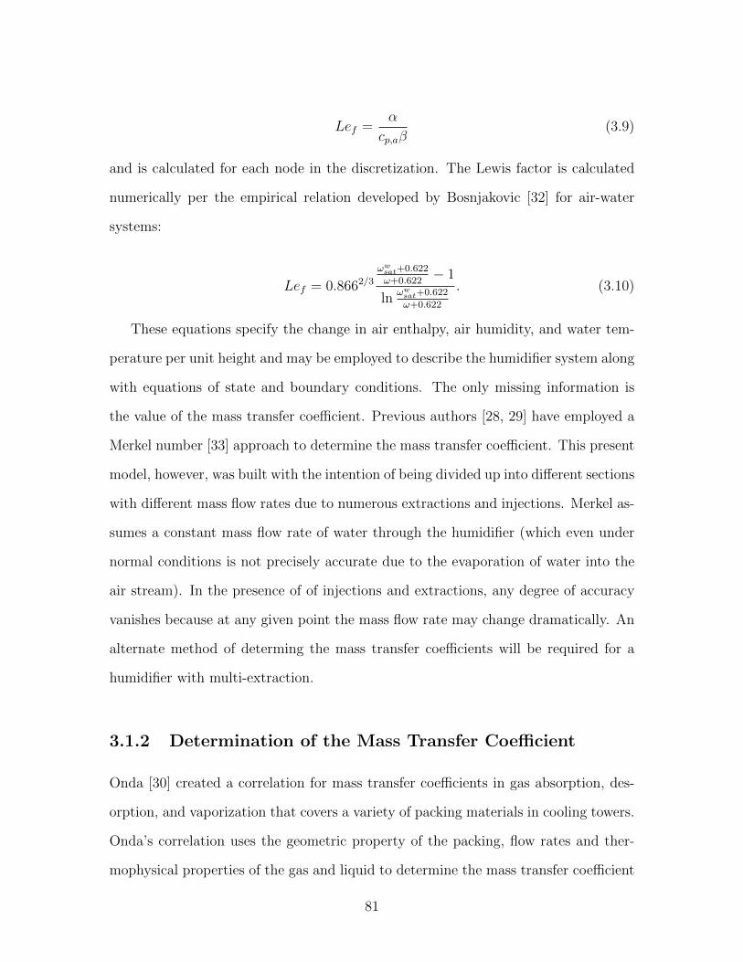
Lef =α
cp,aβ(3.9)
and is calculated for each node in the discretization. The Lewis factor is calculated
numerically per the empirical relation developed by Bosnjakovic [32] for air-water
systems:
Lef = 0.8662/3
ωwsat+0.622
ω+0.622− 1
lnωwsat+0.622
ω+0.622
. (3.10)
These equations specify the change in air enthalpy, air humidity, and water tem-
perature per unit height and may be employed to describe the humidifier system along
with equations of state and boundary conditions. The only missing information is
the value of the mass transfer coefficient. Previous authors [28, 29] have employed a
Merkel number [33] approach to determine the mass transfer coefficient. This present
model, however, was built with the intention of being divided up into different sections
with different mass flow rates due to numerous extractions and injections. Merkel as-
sumes a constant mass flow rate of water through the humidifier (which even under
normal conditions is not precisely accurate due to the evaporation of water into the
air stream). In the presence of of injections and extractions, any degree of accuracy
vanishes because at any given point the mass flow rate may change dramatically. An
alternate method of determing the mass transfer coefficients will be required for a
humidifier with multi-extraction.
3.1.2 Determination of the Mass Transfer Coefficient
Onda [30] created a correlation for mass transfer coefficients in gas absorption, des-
orption, and vaporization that covers a variety of packing materials in cooling towers.
Onda’s correlation uses the geometric property of the packing, flow rates and ther-
mophysical properties of the gas and liquid to determine the mass transfer coefficient
81

as follows:
β = ρvCRe0.7GASc
13G(adp)
−2aDG (3.11)
where
ReGA =G
aµG
(3.12)
ScG =µG
ρGDG
(3.13)
DG = 1.87 ∗ 10−10 (Ta + 273.15)2.072
P101.325
(3.14)
dp is the diameter of a packing bead, C is a geometric coefficient, 5.23 for dp > 0.015
or 2 for dp < 0.015, and DG is the diffusion coefficient from water to air (with Ta
in ◦C Celsius and P in kPa). Using this correlation enables a determination of the
mass transfer coefficient at any height within the humidifier. If directly upstream
or downstream of an extraction, the change in mass flow affects the mass transfer
coefficient. Thus, a different mass transfer coefficient is found at every node within
the discretization of the component.
3.1.3 Solution of Humidifier Model
Utilizing the set of differential equations describing the humidifier, Equations 3.6,
3.7, 3.8, as well as the Onda correlation, Equation 3.11, a finite difference model
of the humidifier may be constructed. Necessary inputs include inlet water and air
temperatures, inlet air humidity, mass flow rates of air and water, humidifier height
and cross-sectional area, packing nominal diameter, and fill specific surface area. To
solve the model, the humidifier must be divided into a number of discrete nodes and
the outlets of each node tied to the inlets of the adjacent node as shown in Figure
3-2. With this input criteria, the model is fully defined (N equations, N unknowns)
82

and may be solved. This model is a two point boundary value problem where some,
but not all, conditions are known at one point, and some conditions are known at
the other. In this case, water temperature and mass flow is known at the top of
the device while air temperature, mass flow, and humidity is known at the bottom.
These types of problems are typically solved with an iterative approach. Whereas
other authors typically solve this system of equations with an iterative mathematical
model [34], here, given appropriate guess values, the EES software [31] automatically
iterates until it finds the solution. Figure 3-3 illustrates a temperature profile for a
humidifier solved with the inputs listed in Table 3.1.
dz
dz
��,�[�]
ℎ�,�[�]
��,�[�+1]
ℎ�,�[�+1]
��,�[�]
ℎ�,�[�]
��,�[�+1]
ℎ�,�[�+1]
Node �
Node � + �
��,�[�]
ℎ�,�[�]
��,�[�+1]
ℎ�,�[�+1]
��,�[�]
ℎ�,�[�]
��,�[�+1]
ℎ�,�[�+1]
Linked Linked
+z
+z
Figure 3-2: Linking of cells in the humidifier model
83
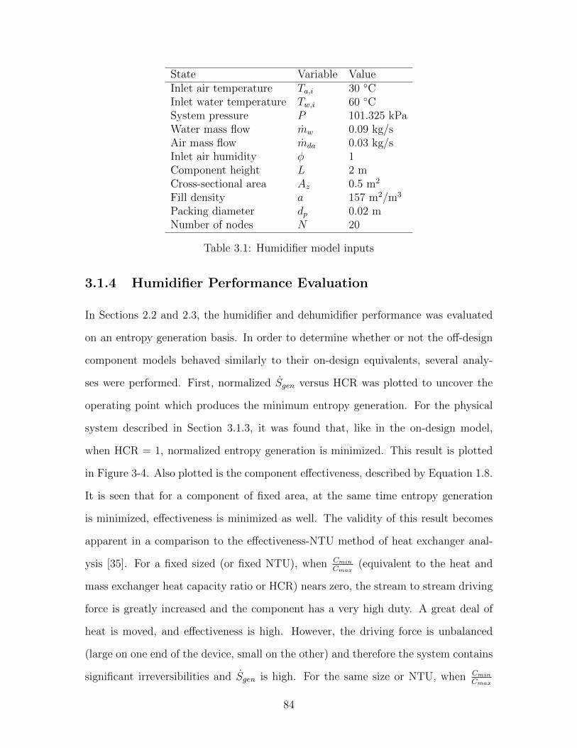
State Variable ValueInlet air temperature Ta,i 30 ◦CInlet water temperature Tw,i 60 ◦CSystem pressure P 101.325 kPaWater mass flow mw 0.09 kg/sAir mass flow mda 0.03 kg/sInlet air humidity φ 1Component height L 2 mCross-sectional area Az 0.5 m2
Fill density a 157 m2/m3
Packing diameter dp 0.02 mNumber of nodes N 20
Table 3.1: Humidifier model inputs
3.1.4 Humidifier Performance Evaluation
In Sections 2.2 and 2.3, the humidifier and dehumidifier performance was evaluated
on an entropy generation basis. In order to determine whether or not the off-design
component models behaved similarly to their on-design equivalents, several analy-
ses were performed. First, normalized Sgen versus HCR was plotted to uncover the
operating point which produces the minimum entropy generation. For the physical
system described in Section 3.1.3, it was found that, like in the on-design model,
when HCR = 1, normalized entropy generation is minimized. This result is plotted
in Figure 3-4. Also plotted is the component effectiveness, described by Equation 1.8.
It is seen that for a component of fixed area, at the same time entropy generation
is minimized, effectiveness is minimized as well. The validity of this result becomes
apparent in a comparison to the effectiveness-NTU method of heat exchanger anal-
ysis [35]. For a fixed sized (or fixed NTU), when Cmin
Cmax(equivalent to the heat and
mass exchanger heat capacity ratio or HCR) nears zero, the stream to stream driving
force is greatly increased and the component has a very high duty. A great deal of
heat is moved, and effectiveness is high. However, the driving force is unbalanced
(large on one end of the device, small on the other) and therefore the system contains
significant irreversibilities and Sgen is high. For the same size or NTU, when Cmin
Cmax
84

Figure 3-3: Temperature and humidity profiles in the humidifier
approachs 1, the variation is driving force is minimized. This corresponds to a small
amount of irreversibility and lower entropy generation. However, by minimizing the
variation is driving force, the driving force itself becomes smaller and the duty of
the component is reduced. Thus, for the same component, there is less heat transfer
and the effectiveness of the device drops. To increase effectiveness in this case, big-
ger hardware must be employed (larger NTU) to reach the larger duty. Thus, high
effectiveness hardware that has minimal entropy generation must be quite large.
Relatedly, it bears mentioning that when the size of the humidifier is increased
significantly (from H = 1 to H = 3.7 and from Az = 0.5 to Az = 1.5), the effectiveness
is increased by over 10% to 0.8 when HCR = 1. This is the typical effectiveness used
in the on-design studies in Chapter 2. In this case, the normalized entropy production
drops to 0.000241. This result differs from the on-design case presented in Figure 2-2
by only 2%. The normalized entropy generation minimized at 0.000236 for the on-
85

Figure 3-4: Entropy production and effectiveness in the humidifier model
design model with zero extractions. In Figure 3-4, the entropy production was about
three times larger at HCR = 1. Thus, to achieve the approximately 2/3 reduction
in entropy production, the humidifier size was increased by about a factor of 11x, a
considerably larger and more expensive piece of equipment.
3.1.5 Validation of Humidifier Model
The humidifier model was validated by comparing analytical results from the model
to experimental data gathered by Sharqawy and Husain [36, 37]. The humidifier code
was modified to match conditions given by Sharqawy and Husain. It was altered to
match the geometry used in the experimental studies and was given different flow
rates and temperatuers. Namely, the humidifier size was reduced to 0.6 m tall by
0.15 wide by 0.15 long with a specific fill area of 110 m2/m3. Though the data covers
both fresh and salt water runs, only runs where fresh water was used were compared
86

Sharqawy [36, 37] Present Work Errormr Ta,o Twb,o Tw,o Ta,o Twb,o Tw,o Ta,o Twb,o Tw,o
- ◦C ◦C ◦C ◦C ◦C ◦C % % %1.0 25.8 23.7 25.5 25.8 24.0 25.6 0.0% 4.8% 1.7%1.5 26.9 24.0 27.1 26.5 23.8 27.5 -8.5% -2.5% -9.3%2.0 27.6 24.5 28.2 27.1 24.6 28.4 -5.5% 1.2% -6.2%
Table 3.2: Humidifier model validation
to minimize errors due to salinity. Initially, the experimental data did not match the
model data. This mismatch was caused by the Onda correlation generating very low
( 0.001 kg/m2-s) mass transfer coefficients. When the Onda correlation was replaced
by a Merkel approach, mass transfer coefficients increased dramatically (to around
0.02-0.03 kg/m2-s) and the data correlated well as illustrated in Table 3.2. Error was
calculated as
Error =∆Tmodel − ∆Texp
∆Texp(3.15)
where ∆T is the change between inlet and outlet temperature. Error was found to
be small: typically under ±5% and no more than ±10%.
It was clear that the Onda correlation did not match experimental data for the
range of inputs employed by Sharqawy and Husain. These boundary conditions were,
however, considerably different than those employed in the humidifier model. Par-
ticularly, temperatures were very low and the size of the humidifier was quite small.
To ensure that Onda’s correlation was valid for the conditions being examined in the
HDH system, another comparison was made.
Onda’s correlation is a general correlation, and per Section 3.1.1, it is clear that the
value of β, the mass transfer coefficient, is strongly linked to the change in temperature
and humidity for a given cell. As such, a simple test was run to determine the
accuracy of β and ensure the correlation’s validity for the humidifier model. The
model was run at several values of mass flow ratio for a given set of input conditions
and the value of β computed for each case. This data was in turn compared to known
87

values of β: data from performance curves of a Brentwood CF-1900SB/MA packing
for counterflow cooling towers [38]. The performance curve gives a single value of
β for the full cooling tower. This value was found to be consistently between the
minimum and maximum values computed along the length of the humidifier in the
model. Note that in the model, a new mass transfer coefficient is found for each
cell based on the local air and water properties. While the Brentwood data tended
toward the lower range of mass transfer coefficients found in the model (see Figure
3-5), it was reasonably close to the average value for mass flow rate ratios in the
system operating range (about 1-3). Thus, the mass transfer coefficient values are
accurate for the humidifier model and model output is considered valid.
Figure 3-5: Comparison of actual and calculated mass transfer coefficients
3.2 Finite Difference Dehumidifier Model
The finite difference dehumidifier was constructed as a tube in tube model [20]. From
literature, this is similar in scope to the finned tube used by Al-Hallaj et al. [39].
88

This is not a compact dehumidifier design such as the finned tubes utilized by El-
Agouz et al. [40] or the flat-plate exchanger employed by Muller-Holst et al. [41].
It was chosen as a simple model where extraction points would be easy to locate on
a single length of tube. It is a 1D counterflow, non-contacting dehumidifier model
that is formulated by a set of differential equations. The differential equations are
reproduced numerically in Engineering Equation Solver (EES) [31] to illustrate the
state of the air or water stream at a specified height within the dehumidifier.
3.2.1 Control Volume Analysis
Figure 3-6 illustrates the control volume in the counterflow dehumidifier. From Figure
3-6, the mass balance may be described by
Dehumidifier / Condenser
Inspection Node dz
�� + ���ℎ� + �ℎ�
��ℎ�
��� 1 + � + ��ℎ� + �ℎ�
��� 1 + �ℎ�
��ℎ�
+z
Figure 3-6: Control Volume of Counterflow Dehumidifier
mdadω
dz= dmd (3.16)
while the energy balance is given by
hwdmw
dz+ mw
dhwdz
= mdadhadz
+ dmdhd. (3.17)
89

The heat and mass transfer equations for the tube in tube dehumidifier can be
derived from a simple resistor network realization. Per Figure 3-7, a series of equa-
tions derived from these resistances is utilized to determine temperatures. Resistances
emerge from the air to film convective resistance (which includes a parallel current for
latent heat moved through mass transfer), a film conductive resistance, a wall con-
ductive resistance, and a wall to water convective resistance. Additionally illustrated
in Figure 3-7 is the mass transfer resistance from film to bulk air stream.
Figure 3-7: Resistance network model for dehumidifier
dQ
dAs
= hc,a(Ta − Ti) +md
dAs
hfg (3.18)
dQ
dAs
= hc,w(Tww − Tw) (3.19)
dQ
dAs
= 2kwallD12 ln
(D2
D1
)(Taw − Tww) (3.20)
dQ
dAs
= 2kfilmD23 ln
(D3
D2
)(Tint − Taw) (3.21)
dmd
dAs
= β(xa − xint) (3.22)
It should be noted Equation 3.22 is only active for when the air side wall temperature,
90

Taw, is lower than the dewpoint temperature of the bulk airstream, Tdp. When Taw >
Tdp no condensation can occur and the flow rate of distillate, md, is zero.
Heat transfer coefficients are calculated assuming fully developed internal flow
within pipes or annuli. A new heat transfer coefficient is found for each cell based on
local fluid properties. The coefficient is given by
NuD =αDh
kf(3.23)
where Nu is the Nusselt number, Dh the hydraulic diameter of the pipe, α is the heat
transfer coefficient, and kf the thermal conductivity of the fluid exchanging heat to
the surface. In turn, the Nusselt number is calculated via the Dittus-Boelter equation
[42], a good approximation for the dehumidifier in which the bulk fluid temperature
is close to the heat transfer surface temperature and the Reynolds number is within
10,000 to 120,000:
NuD = 0.023Re45DPr
n (3.24)
where n = 0.4 for heating of the fluid (in this case, water) and n = 0.3 for cooling
(air).
The mass transfer coefficient is then calculated from the heat transfer coefficient
employing the Chilton-Colburn J-factor analogy [42].
α
ρV cpPr
23 =
Cf
2=β
VSc
23 (3.25)
3.2.2 Solution of Dehumidifier Model
Utilizing the set of differential equations describing the dehumidifier, Equations 3.16
through 3.25, a finite difference model of the dehumidifier may be constructed. Nec-
essary inputs include inlet water and air temperatures, inlet air humidity, mass flow
rates of air and water, dehumidifier height and cross sectional area. Additionally, the
91

dehumidifier must be divided into a number of discrete inspection sections and the
outlets of each cell tied to the inlets of the adjacent cell per Figure 3-8. Here, the
model is fully defined (N equations, N unknowns) and may be solved. This model
is a two point boundary problem where some conditions are known at one side of
the dehumidifier while some conditions are only known on the other side. In this
case, water temperature and mass flow is known at the bottom of the device while
air temperature, mass flow, and humidity is known at the top. These types of prob-
lems are typically solved with an iterative approach. Here, given appropriate guess
values, the EES software [31] automatically iterates until it finds the solution. Figure
3-9 illustrates temperature and humidity profiles for a dehumidifier solved with the
inputs listed in Table 3.3.
dz
��,�[�+1]
ℎ�,�[�+1]
��,�[�+1]
ℎ�,�[�+1]
��,�[�+1]
ℎ�,�[�+1]
��,�[�+1]
ℎ�,�[�+1]��[�+1]
ℎ�[�+1]
dz
��,�[�]
ℎ�,�[�]
��,�[�]
ℎ�,�[�]
��,�[�]
ℎ�,�[�]
��,�[�]
ℎ�,�[�]
��[�]
ℎ�[�]
LinkedLinked
Node �
Node � + �
+z
+z
Figure 3-8: Linking of cells in the dehumidifier model
92

State Variable ValueInlet water temperature Tw,i 30 ◦CInlet air temperature Ta,i 60 ◦CSystem pressure P 101.325 kPaWater mass flow mw 0.081 kg/sAir mass flow mda 0.03 kg/sInlet air humidity φ 1Component length L 50 mWater pipe cross-sectional area Aw 0.00011 m2
Air pipe cross-sectional area Aa 0.0019 m2
Total heat transfer area As 1.875 m2
Number of nodes N 50
Table 3.3: Dehumidifier model inputs
3.2.3 Dehumidifier Performance Evaluation
Similarly to Section 3.1.3, normalized Sgen versus HCR was plotted to determine the
operating point which produces the minimum entropy generation. For the physical
system described in Section 3.2.2, it was found that, like in the on-design model,
when HCR = 1, normalized entropy generation is minimized. This result is plotted
in Figure 3-10. Also plotted is the component effectiveness, described by Equation 1.8.
It is seen that for a component of fixed area, at the same time entropy generation
is minimized, effectiveness is minimized as well. As in Section 3.1.4, this result is
validated by the effectiveness-NTU analysis of a similar heat exchanger. Again it is
seen that to increase effectiveness larger hardware must be employed (larger NTU)
to reach a larger duty. Thus, high effectiveness hardware that has minimal entropy
generation will be quite large.
When the model is altered to operate at the same inlet conditions as the off
design dehumidifier, the normalized entropy production is 0.00464 at HCR = 1 and
εD = 0.8. This result is very similar to the on-design case presented in Figure 2-4
where the normalized entropy generation minimized at 0.00491 for the case with zero
extractions.
93

Figure 3-9: Temperature and humidity profiles in the dehumidifier
3.2.4 Dehumidifier Validation
For the humidifier, cooling tower experimental data may be leveraged to validate the
code. For the dehumidifier, however, due to the relatively simplistic and inefficient
concentric tube design, a literature review yielded no solid experimental data that
matches the conditions utilized in this model. Again, the concentric tube dehumidifier
was chosen to simplify the model, particularly with regards to adding extractions at
known locations. To validate the model, a few limiting cases were analyzed to compare
the model against known points typically found in literature. For instance, a run was
performed where the inlet air humidity was brought to zero. With completely dry
air as one stream, and water as the other, the problem reduces to a simple heat
exchanger. No condensation forms in this run, so there is no mass transfer. A run
was evaluated at the conditions in Table 3.4.
This run yielded an effectiveness of εD = 0.755 and a Cmin
Cmaxor HCR of 1. Per a
standard effectiveness-NTU model of a counterflow, concentric tube heat exchanger
[35], this effectiveness should yield NTU as
94

Figure 3-10: Entropy production and effectiveness in the dehumidifier model
NTU =ε
1 − ε. (3.26)
Thus, NTU = 3.08. To validate the model then, NTU was reproduced analytically.
First, the log mean temperature was calculated from inlet and outlet conditions of
the air and water stream:
∆Tlm =∆Thot − ∆Tcold
ln ∆Thot
∆Tcold
(3.27)
∆Tlm =(70.0 − 59.1) − (39.8 − 30.0)
ln 70.0−59.139.9−30.0
(3.28)
∆Tlm = 10.3◦C (3.29)
The log mean temperature was used to find U , the overall heat transfer coefficient
95

State Variable ValueInlet water temperature Tw,i 30 ◦CInlet air temperature Ta,i 70 ◦CSystem pressure P 101.325 kPaWater mass flow mw 0.0125 kg/sAir mass flow mda 0.05 kg/sInlet air humidity φ 0.0Component length L 100 mWater pipe cross-sectional area Aw 0.00011 m2
Air pipe cross-sectional area Aa 0.0019 m2
Total heat transfer area As 3.75 m2
Number of nodes N 50
Table 3.4: Dehumidifier validation inputs - zero humidity case
for the dehumidifier
U =Q
∆TlmAs
(3.30)
U =(1521 W)
(3.75 m2)(10.3 ◦C)(3.31)
U = 39.2 W/m2 − K (3.32)
which was then used to calculate NTU:
NTU =UA
Cmin
(3.33)
NTU =(39.2 W/m2 − K)(3.75 m2)
(50.3 W/K)(3.34)
NTU = 2.96 (3.35)
This value of NTU agrees with the original calculated value to within 4%. This result,
then, supports the validity of the dehumidifier model. Another run was performed
where mda >> mw. In this case, the temperature of the wall between the streams
stays constant at the air side temperature. The system reduces to a single stream
exchanger where
96

State Variable ValueInlet water temperature Tw,i 40 ◦CInlet air temperature Ta,i 60 ◦CSystem pressure P 101.325 kPaWater mass flow mw 0.05 kg/sAir mass flow mda 0.50 kg/sInlet air humidity φ 1.0Component length L 50 mWater pipe cross-sectional area Aw 0.00011 m2
Air pipe cross-sectional area Aa 0.0019 m2
Total heat transfer area As 1.875 m2
Number of nodes N 50
Table 3.5: Dehumidifier validation inputs - single exchanger case
ε = 1 − e−NTU (3.36)
Using the parameters found in Table 3.5, this run yielded an effectiveness of
εD = 0.9485 and per Equation 3.36, NTU = 2.967. A repeat of the mathematics laid
out in Equations 3.27, 3.30, and 3.33 yielded a log mean temperature of Tlm = 6.32, an
overall heat transfer coefficient of U = 334.8, and a calculated NTU of NTU = 3.002.
The error between estimated and calculated NTU was then under 1.2%. Again, this
limiting case lends creditability to the validity of the model.
3.3 Full Cycle Model
A full HDH system is constructed by using the humidifier model from Section 3.1 and
the dehumidifier model from Section 3.2. Some input variables are removed and the
outputs of the two models are tied together. For instance, as the cycle is a closed air
open water cycle (CAOW), the air outlet of the dehumidifier is linked to the air inlet
of the humidifier. Thus, hD,a,o = hH,a,i, mD,da,o = mH,da,i, and ωD,a,o = ωH,a,i.
97

Component Heat Transfer Area Length/Height Cross Sectional Area[m2] [m] [m2]
Dehumidifier 4.88 130 0.0019Humidifier 455 2.9 1
Table 3.6: High GOR water-heated HDH cycle component data
3.3.1 Water-Heated System Model
In constructing a water-heated model, the inlet water temperature to the humidifier
is specifed, as is the cold water inlet to the dehumidifier. Thus, the dehumidifier air
outlet is linked to the humidifier air inlet. The water streams are not linked; the
water temperature into the humidifier is specified and the dehumidifier water outlet
temperature is allowed to float. The energy input into the cycle is determined by
Qin = mw(hH,w,i − hD,w,o). (3.37)
Mistry et al. [43] described a high performance water heated HDH cycle utilizing
very high values of effectiveness. For instance, a cycle with the dehumidifier effec-
tiveness, εD = 0.96 and humidifier effectiveness, εH = 0.92 at an optimal mass flow
rate ratio had a GOR peaking near 4.9. This system was based on an on-design,
fully thermodynamic model, so component sizes were not known or given. As this
information is necessary in building a system, the off-design model developed in this
section was used to replicate the cycle and determine the feasibility of building such
a system. Representative values for the system are shown in Table 3.6. The per-
formance of the system matches very closely with the model given by Mistry [43] as
seen in Table 3.7. GOR and entropy generation values are very similar. The only key
difference between the two models are the values of effectiveness which were higher
in Mistry’s model.
In Table 3.6 it became apparent that achieving a high GOR would nominally
require a system of considerable size, particularly with regards to the humidifier. The
98

Parameter Mistry On Design[43] Off DesignGOR 4.87 4.86TTD 2.0 2.2Sgen [kW/K] 0.15 0.16mr 2.44 2.44εD 0.96 0.94εH 0.93 0.85Tmin [◦C] 30.0 30.0Tmax [◦C] 58.6 58.6
Table 3.7: Comparison of high GOR water-heated HDH cycles
humidifier used to obtain these cycle parameters was 2.9 m in height. To assess
the impact of different component sizes on GOR, an additional series of runs was
performed while varying humidifier and dehumidifier size. The results are plotted in
Figure 3-11.
In these runs, the peak GOR was obtained by varying the mass flow rate ratio, mr,
only. Peak GOR typically occurred for 1.9 < mr < 2.3. From the figure, it becomes
apparent that high GOR is a very strong function of component size. However, both
components are important factors in GOR. For a smaller humidifier of volume 1.7 m3
(cross sectional area = 1 m2, height = 1.7 m) GOR ranged from about 2.1 to 3.6 by
significantly varying the size of the dehumidifier. Based on the curvature of the data,
it does not appear that the GOR will be able to surpass much more than 4 even if an
extremely large dehumidifier is employed. These diminishing returns on component
size were also shown, in terms of water production, by Nawayseh et al. [44]. For a
large humidifier of volume 3.5 m3, GOR had a much larger range: from 2.7 to 6.9. The
presence of the larger humidifier enabled a large dehumidifier to have more impact
on GOR. Doubling the size of the dehumidifier from 1.5 m2 to 3.0 m2 nearly doubles
GOR. Thus, it is clear that larger components can yield very high performance and
reduce the energy requirements of the HDH system considerably. However, it should
be noted that in this series of runs, water production rate varied from 0.0016 kg/s
99

Figure 3-11: Peak GOR versus component size
to 0.0027 kg/s at a GOR of 2.1 and 6.9 respectively. So while the GOR more than
tripled, water production rate increased by only about 70%. Therefore, this increase
in component size is doing more to reduce Qin than increasing md. In Figure 3-
12, water production is plotted against total humidifier and dehumidifier volume. It
appears that water production rate follows a logarithmic function. For small systems,
increasing size has a large impact on the water production rate, but larger systems get
significantly diminishing returns. Increasing component size decreases the pinch at
the hot side of the dehumidifier (thereby reducing the ∆T the water must go through
in the heater, and correspondingly reducing Qin) but is not reducing the pinch at the
cold side as much (therefore ω at the cold side of the device is not as low and the
∆ω through the dehumidifier is not as large). Clearly, system size has a very strong
relationship with the amount of energy needed to run the cycle, but a weaker response
in terms of water production. In designing an HDH system, there is a considerable
100

trade off between overall performance and the amount of water production.
Figure 3-12: Water production rate versus system size for various humidifier anddehumidifer sizes
3.3.2 Air-Heated System Model
In the case of an air-heated cycle, the dehumidifier air inlet temperature is specified,
as is the cold water inlet temperature. In this case, the air stream is not linked, but
the water stream (dehumidifier outlet to humidifier inlet) is linked. The energy input
is specified by
Qin = mda(hD,da,i − hH,da,o). (3.38)
While it was possible to emulate Mistry’s water heated cycle, the air heated cy-
cle produced considerably more difficulty. For the air heated cycle, the model was
unable to replicate the high GOR cycle. This result was largely due to convergance
issues in the model when utilizing very large components (to achieve high values of
101

Parameter Mistry On Design[43] Off DesignGOR 7.76 3.14TTD 2.0 1.7Sgen [kW/K] 0.15 0.38mr 2.12 2.10εD 0.98 0.96εH 0.96 0.87Tmin [◦C] 30.0 30.0Tmax [◦C] 90.0 90.0
Table 3.8: Comparison of two different air-heated HDH cycles
effectiveness). The high levels of effectiveness were unable to be obtained utilizing
the current model. However, an air heated cycle was run that resulted in a GOR of
3.14 per Table 3.8.
3.4 Extractions in Off-Design Model
Like in the on-design model, it is possible to improve system efficiency via extractions
and injections. Using the high performance water heated cycle discussed in Section
3.3.1 as a baseline, a single water extraction is made. Water is extracted from the
dehumidifier at the local bulk water temperature of the node outlet. It is then injected
into the humidifier at the same temperature to minimize entropy generation from
mixing losses. This is modeled by removing water downstream of the oulet of a node,
and upstream of the next node. To ensure temperatures match at both the extraction
and injection sites, the nodes are iterated upon until the temperatures match. Several
extractions were made along the length of the dehumidifier to compare the impact of
extracting at a different location. Because the extraction and injection temperatures
were required to match, it was not possible to extract at the very bottom of the
dehumidifier as this water was cooler than water at any location in the humidifier. It
is possible, however, to extract near the top and middle of the component at higher
water temperatures. A compilation of extraction data is illustrated in Table 3.9. It
102

Flow extracted Extraction temperature GOR% circut flow ◦C -0% – 5.3310% 55.4 5.5010% 50.6 5.4910% 46.5 5.3210% 40.5 5.2320% 53.1 5.6520% 50.1 5.6220% 45.6 5.1420% 40.3 4.84
Table 3.9: Impact of extraction on high GOR water-heated cycle
was seen that extracting water at relatively high temperature from the dehumidifier
(extraction location at approximately 80% dehumidifier height) and injecting it very
close to the top of the humidifier (at the same temperature and therefore enthalpy)
produced a reasonably large increase in performance. Like with many of the on-
design cycles, it was also apparent that for extracting at a fixed location, there is
often an ideal extraction rate that achieved the highest GOR. In Figure 3-13, GOR
was improved to 5.4 from the baseline of 4.9 via a 40% extraction in water flow (.029
kg/s) at approximately 50 ◦C.
Also plotted in Figure 3-13 is the normalized stream to stream variance. An
important advantage of this off-design study over the on-design studies is that full
temperature and humidity profiles may be developed for the entire length of the hu-
midifier and dehumidifer. Tondeur et al. [45] proposed that the optimal method of
reducing entropy production within a contacting or separation device was to “equipar-
tition” the entropy generation such that entropy production is evenly distributed
along the length of the device. The fundamental motivation here is that in equipari-
tion, all entropy producing driving forces are uniform (specifically, the variance is
zero). Tondeur and Thiel et al. [45, 20], who recently extended this concept to HDH
dehumidifiers, show that when the variance reaches zero, entropy production is min-
imized. For both humidifiers and dehumidifiers, the driving forces in question are
103
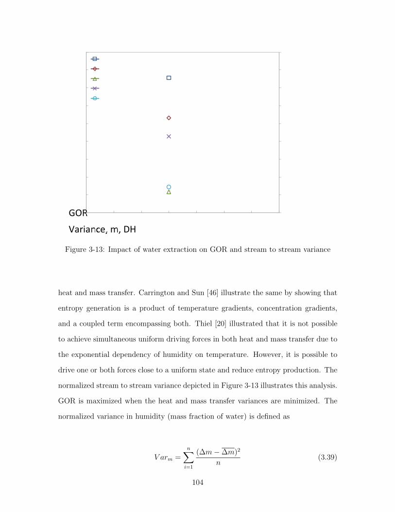
Figure 3-13: Impact of water extraction on GOR and stream to stream variance
heat and mass transfer. Carrington and Sun [46] illustrate the same by showing that
entropy generation is a product of temperature gradients, concentration gradients,
and a coupled term encompassing both. Thiel [20] illustrated that it is not possible
to achieve simultaneous uniform driving forces in both heat and mass transfer due to
the exponential dependency of humidity on temperature. However, it is possible to
drive one or both forces close to a uniform state and reduce entropy production. The
normalized stream to stream variance depicted in Figure 3-13 illustrates this analysis.
GOR is maximized when the heat and mass transfer variances are minimized. The
normalized variance in humidity (mass fraction of water) is defined as
V arm =n∑
i=1
(∆m− ∆m)2
n(3.39)
104

where
∆m =ma −mi
Average(ma −mi)(3.40)
and normalized variance in temperature is defined as
V arT =n∑
i=1
(∆T − ∆T )2
n(3.41)
where
∆T =(Ta − Ti)
Average(Ta − Ti). (3.42)
The variance is a measure of the uniformity of the stream to stream driving force.
In the case of the dehumidifier shown in Figure 3-13, the variance in humidity com-
pares the humidity of the bulk air stream to that of the air water interface of the
condensate. The variance in temperature compares the bulk air temperature to that
of the condensate interface. For the humidifier, the humidity variance comes from
the difference between bulk air and humidity at the liquid/air interface on the fill.
Temperature variance measures the bulk air temperature and interfacial temperature
on the fill. Clearly the variance in the mass transfer is the larger of the two, though
GOR appears to minimize where both variances reach a relative minimum in the de-
humidifier. For the humidifier, increasing extraction appears to increase the variance
in both m and T . This is also reflected in the HCR, which grows from 1.15 to 1.34
at 40% extraction rate. Figure 3-13 confirms that, like the on-design studies, it is
the dehumidifier that is driving the system performance more so than the humidifier.
Again similar to on-design, by extracting and balancing the dehumidifier, the humid-
ifier performance worsens. However, as seen in Figure 3-13, the variance in m and T
for the humidifier is much smaller at low extraction rates and does not become larger
than the dehumidifier until after the peak GOR value is reached. At the peak GOR,
the dehumidifier has reached a peak performance while the humidifier performance
worsens. To the right of peak GOR, the humidifier entropy generation begins to drive
105

the system performance and GOR quickly drops in response.
106

Chapter 4
Conclusions
Thermodynamic system balancing by way of multi-extraction is a clear and effective
method to increase the performance of an HDH system without necessarily changing
equipment size. While it is true that increasing the equipment size (and therefore
effectiveness) for the humidifier and dehumidifier of an HDH system is perhaps the
most straight forward method of improving system performance, for an existing sys-
tem, single or multiple fluid extractions can be made to increase performance (GOR)
considerably.
Both on and off design studies did not generate many sweeping generalizations
for multi-extraction, but many critical ideas were assessed and evaluated and highly
useful results were obtained.
4.1 On-Design Lessons Learned
• First, it was confirmed that driving the system toward HCR = 1 either by wayof adjusting the mass flow rate ratio, mr, or via extractions significantly reducesentropy generation, Sgen and increases GOR.
– When the system is split into multiple subcomponents, adjusting the ex-traction rate between the components such that HCR = 1 for the compo-nents with the largest Sgen is the best method to improve performance.
107

– Optimally, adjusting extractions and injections to force HCR = 1 for allsubcomponents should yield an exceptionally high performance system.
• Next, for all single extraction systems, performance was optimized by extractingand injecting from the stream with the maximum capacity rate.
– For example, when mr is large and the water stream has the maximumcapacity rate, a larger performance gain was realized by extracting water.
– Conversely, a system with a small mr with air at the maximum capacityrate had improved performance when air was extracted.
• Finally, it was found that in the majority of cases, multiple extractions improvedperformance moreso than a single extraction.
– This statement is particularly true for systems with low TTD (and higheffectiveness).
– While multiple extractions produce higher performance, it was also de-termined that the first extraction typically resulted in the highest perfor-mance gain, while subsequent extractions yielded diminishing returns. Indesigning an HDH system with multiple extractions, it is clear that therewill be a trade off between the cost and the performance gain of the Nthextraction.
4.2 Off-Design Lessons Learned
• Like in heat exchangers, for a fixed area component, entropy minimization oc-curs at the same cycle condition as the minimum effectiveness. Therefore, tohave a high performance system (both high effectiveness and low entropy gen-eration) the equipment utilized must be large.
• To reduce the necessary size of equipment to achieve a high GOR system, ex-tractions may be made. Adding extractions to the cycle can allow for a highersystem performance without changing the equipment size. Alternatively, in-creasing both system size and the number of extractions can generate evenhigher GOR cycles.
• High GOR cycles (of up to 6-7) are possible in the water-heated configuration.These cycles require large equipment (3-4 m tall humidifier) and will not producesignificantly more product water than a lower GOR case. However, the energyinput requirement of these cycles drops dramatically (from 1.78 to 0.94 kWthermal for a GOR of 6.90 and 2.17 respectively). This sharp reduction in heatinput could significantly rescale the size of a solar collector if the HDH is to bepowered by solar thermal energy, or could reduce the amount of steam leeched
108
from a power generation cycle to run the system. In designing an HDH system,cost of the solar collector needs to be weighed against costs of the humidifier anddehumidifier. It may be that an optimum point exists in terms of minimizingenergy intensity or maximizing water production.
• GOR is directly and strongly related to both the humidifier and dehumidifiersize. It is possible to increase the dehumidifier size, for instance, to improveGOR but as the size increases, there will be diminishing returns. Eventuallythere is no benefit from increasing dehumidifier size without increasing the hu-midifier size simultaneously.
• Extractions boost system performance by minimizing entropy generation. En-tropy generation is minimized by minimizing the variation in stream to streamhumidity and temperature profiles. While both temperature and humidity areimportant, it is the humidity that typically has the largest variation, often bya factor of 5-7x. Therefore, while both profiles should be made parallel viaextractions for optimum performance, humidity is the more desirable target.
4.3 Future Work
While numerous on and off-design cycles were analyzed in this study, a more gener-
alized relationship between performance, entropy generation, and extractions will be
developed. Key principles and ideas regarding extraction were assessed, but a quick
yet rigorous model must be created than can easily predict the optimal extraction
locations and flow rates based on any input system or cycle. This thesis showed a
significant amount of overlap between the on and off design models which validates
the theory. So while a simple thermodynamic model (on-design) would be adequate
to begin the optimization, a full off-design model with extractions is a more rigor-
ous way of evaluating real hardware. As seen in the off-design studies, some cycles
(particularly air-heated cycles) are considerably more difficult to reproduce with ac-
tual hardware. While thermodynamically feasible, some of these cycles would require
significantly more advanced hardware to meet the required heat and mass transfer
characteristics. High GOR HDH cycles with significantly smaller energy inputs have
been identified, but with a more complete multi-extraction off-design model, it is
109

likely that even higher performance systems may be obtained.
There may be an optimum design for an HDH system based on dollars per kg
of water or in terms of energy input. Increasing humidifier and dehumidifier size
in order to boost system performance requires a smaller solar collector. However,
the increase in GOR does not scale 1:1 with the amount of water production. If a
system is being evaluated in terms of water production, there likely exists a point
where increasing the system size becomes impractical because the additional amount
of water produced is insufficient to justify the cost. Conversely, if the goal of the
system is to minimize energy use per unit cost, the optimal system size would be
different. Further thermo-economic studies are required to optimize the system on a
given parameter such as production rate or energy use.
4.4 Final Remarks
While HDH systems have existed for many years, there is clearly more optimization
required to bring them up to par with other desalination systems which has been
studied, fine-tuned, and perfected over the last few decades. A basic HDH system
has comparably low performance when placed side by side with a large MED or MSF
plant. However, by way of these and other studies, it is likely that HDH systems
may be dramatically improved upon in the years to come. Though HDH may not
take the place of existing systems, there are many niche markets, particularly in the
developing world, where a small scale HDH system may be soon become competitive
with other desalination technologies.
110

Appendix A
Comparison of Zero Extraction
Cycles
As discussed in Section 2.4.5, the method by which the on-design model was con-
structed introduces some complications. Specifying the total component effectiveness
is not possible when each is built of two or more subcomponents because doing so
does not generate enough equations and conditions to fully specify the system. Ad-
ditionally, it was found that attempting to specify a total fixed effectiveness when
extractions were involved was not a valid method of analyzing the system. As found
in Chapter 3, the addition of an extraction/injection into the cycle necessarily changes
the total effectiveness of each component. Leaving the total effectiveness fixed, then,
produces a different cycle that cannot be directly compared with the previous. In-
stead, each subcomponent must have a fixed effectiveness specified. This method too
has its own ramifications. Each extraction requires one additional subcomponent.
With each additional subcomponent added in series, the overall effectiveness of the
system increases. As effectiveness directly impacts GOR, these systems will have a
higher GOR, even with the extractions turned off. Thus, as described in Section
2.4.5 each case needs to be handled individually when adding extractions to ensure
111

(a) Water heated cycle (b) Air heated cycle
Figure A-1: Single component HDH Cycles
the move from zero to one to two extractions (etc.) does not alter the performance
of the baseline until the extractions are actually turned on.
Mistry et al. [47] described several on-design models without extraction and also
at a fixed effectiveness. It was found that when a single component cycle without
extraction was run, the models produced for this thesis yielded results nearly identical
to [47] in terms of GOR versus mass flow rate ratio, mr. Figure A-1 illustrates a single
component water heated and air heated cycle each with εD = εH = 0.8. The curve
exhibits the same shape depicted by Mistry. Note that in the air heated cycle, Figure
A-1b, there is a portion of the curve that is marked by a dashed line. These values of
mr produce a cycle that violates the second law, so the system is unable to operate
using those boundary conditions.
When models with additional subcomponents are generated, however, the baseline
GOR vs. mr curve changes considerably. Figure A-2 demonstrates the impact of
increasing the number of subcomponents in the cycle model. The three models in
Figure A-2a share the same input conditions and are not subject to any extractions
or injections; this is the base case. However, the models have either one, two, or
three subcomponents in the humidifier and dehumidifer which considerably changes
the shape of the GOR vs. mr curve. The shape if the curves corresponds to the
112

individual performance of each subcomponent. For instance, each inflection point on
the GOR curves occur when one of the subcomponents’ HCR = 1. In the case of
the single subcomponent model, the inflection at mr = .7 corresponds to HCRD = 1
while the inflection at mr = 1.7 corresponds to HCRH = 1. Similarly, for the three
subcomponent model, the inflection at mr = .4 reflects HCRD1 = 1, the inflection
at mr = 1.75 reflects HCRD2 = 1, and even the small, difficult to see inflection at
mr = 1.9 corresponds to HCRH2 = 1. At these inflections, the minimum capacity rate
changes from one stream to another and the slope of the curve is altered accordingly.
The greater the number of subcomponents in the device, the higher the intial
GOR before extraction is added to the cycle. This is because each subcomponent has
a fixed effectiveness (in this case, εall = 0.8). Therefore, the first subcomponent oper-
ates at an 80% effectiveness and then feeds into a further component operating at 80%
effectiveness, and so forth. This model of the system reduces the “size” of each sub-
component further downstream. If the temperature drop through the first component
is 15 ◦C, the next component may be 10, then 5, etc. because each component is 80%
effective. This series of heat and mass exchangers totals to an equivalent effectiveness
of greater than 80%. Even when there are no extractions, the initial performance of
a three subcomponent system is far superior to a system with a single component
humidifier and dehumidifier. While such a system is still physically conceivable, it is
physically distinct from the previous system in terms of size and architecture. There-
fore, this approach is dissimilar to a laboratory or production design which would
have components of a fixed size, and then injections/extractions would be introduced
to improve the otherwise fixed design. Specifically, the multi-subcomponent method
effectively increases the size of the humidifier and dehumidifier such that each system
can not be directly compared with one another if each individual component has the
same effectiveness. Thus, an off-design analysis of the HDH system is considerably
more feasible and is discussed in Chapter 3.
113

(a) GOR comparison
(b) Effectiveness comparison
Figure A-2: Zero extraction comparison for a 1, 2, and 3 subcomponent air heatedmodel
114

Bibliography
[1] E. Delyannis, “Historic background of desalination and renewable energies,” So-lar Energy, vol. 75, no. 5, pp. 357–66, 2003.
[2] T. Pankratz, IDA Desalination Yearbook 2010-2011, section 1, p. 1. IDA Desali-nation Yearbook, Media Analytics Ltd., 2010.
[3] G. N. Tiwari, H. N. Singh, and R. Tripathi, “Present status of solar distillation,”Solar Energy, vol. 75, no. 5, pp. 367 – 373, 2003.
[4] G. P. Narayan, M. H. Sharqawy, E. K. Summers, J. H. Lienhard V, S. M. Zubair,and M. A. Antar, “The potential of solar-driven humidification-dehumidificationdesalination for small-scale decentralized water production,” Renewable and Sus-tainable Energy Reviews, vol. 14, no. 4, pp. 1187–1201, 2010.
[5] I. Houcine, M. BenAmara, A. Guizani, and M. Malej, “Pilot plant testing ofa new solar desalination process by a multiple-effect-humidification technique,”Desalination, vol. 196, no. 1-3, pp. 105 – 124, 2006.
[6] E. Chafik, “Design of plants for solar desalination using the multi-stag heat-ing/humidifying technique,” Desalination, vol. 168, pp. 55 – 71, 2004.
[7] G. P. Narayan, M. H. Sharqawy, J. H. Lienhard V, and S. M. Zubair, “Ther-modynamic analysis of humidification dehumidification desalination cycles,” De-salination and Water Treatment, vol. 16, pp. 339–353, 2010.
[8] H. Ettouney, “Design and analysis of humidification dehumidification desalina-tion process,” Desalination, vol. 183, no. 1-3, pp. 341 – 352, 2005.
[9] H. Muller-Holst, M. Engelhardt, and W. Scholkopf, “Small-scale thermal sea-water desalination simulation and optimization of system design,” Desalination,vol. 122, no. 2-3, pp. 255–262, 1999.
[10] I. Garaway and G. Grossman, “Investigation of a solar-powered desalinationsystem employing regeneration,” Desalination, vol. 197, no. 1-3, pp. 63 – 74,2006.
[11] P. N. Govindan, M. H. Elsharqawy, J. H. Lienhard V, and S. M. Zubair, “Waterseparation under reduced pressure,” 2011. US Patent number 2011/0056822 A1.
115

[12] H. Jaber and R. L. Webb, “Design of cooling towers by the effectiveness-ntumethod,” ASME Journal of Heat Transfer, vol. 111, pp. 837–843, 1989.
[13] N. P. Cheremisinoff and P. N. Cheremisinoff, Cooling towers: selection, design,and practice. Ann Arbor, MI.: Ann Arbor Science Publishers, 1981.
[14] G. P. Narayan, J. H. Lienhard V, and S. M. Zubair, “Entropy generation mini-mization of combined heat and mass transfer devices,” International Journal ofThermal Sciences, vol. 49, no. 10, pp. 2057–2066, 2010.
[15] G. P. Narayan, K. H. Mistry, M. H. Sharqawy, S. M. Zubair, and J. H. Lien-hard V, “Energy effectiveness of simultaneous heat and mass exchange devices,”Frontiers in Heat and Mass Transfer, vol. 1, no. 2, pp. 1–13, 2010.
[16] A. Bejan, Entropy generation minimization: the method of thermodynamic opti-mization of finite size systems and finite time processes. CRC Press LCL, 1996.
[17] J. H. Lienhard IV and J. H. Lienhard V, A Heat Transfer Textbook. Cambridge,MA.: Phlogiston Press, third ed., 2008.
[18] H. Muller-Holst, “Solar thermal desalination using the multiple effect humidi-fication (meh)-method,” Solar Desalination for the 21st Century, pp. 215–225,2007.
[19] R. Shah, D. Sekulic, and K. (Firm)., Fundamentals of heat exchanger design.Wiley Online Library, 2003.
[20] G. P. Thiel and J. H. Lienhard V, “Entropy generation analysis of a condenserfor use in a humidification dehumidification desalination system.” 2011.
[21] M. H. Sharqawy, J. H. Lienhard V, and S. M. Zubair, “Thermophysical propertiesof seawater: a review of existing correlations and data,” Desalination and WaterTreatment, vol. 16, no. 1-3, pp. 354–380, 2010.
[22] L. Harr, G. S. Kell, and J. S. Gallagher, “Nbs/ncr steam tables,” 1984.
[23] R. H. Hyland and A. Wexler, “Formulations for the thermodynamic properties ofthe saturated phases of h2o from173. 25 k to 473.15 k,” ASHRAE Trans, vol. 89,1983.
[24] D. Wessel, “Ashrae fundamentals handbook 2001 (si edition),” American Societyof Heating, Refrigerating, and Air-Conditioning Engineers, 2001.
[25] K. H. Mistry, “Second law analysis and optimization of humidification-dehumidification desalination cyles,” Master’s thesis, Massachusetts Institute ofTechnology.
[26] M. A. Younis, M. A. Darwish, and F. Juwayhel, “Experimental and theoreti-cal study of a humidification-dehumidification desalting system,” Desalination,vol. 94, no. 1, pp. 11–24, 1993.
116

[27] M. Ben Amara, I. Houcine, A. Guizani, and M. Maalej, “Experimental studyof a multiple-effect humidification solar desalination technique,” Desalination,vol. 170, no. 3, pp. 209–221, 2004.
[28] J. C. Kloppers, A critical evaluation and refinement of the performance predictionof wet-cooling towers. PhD dissertation, University of Stellenbosch, Departmentof Mechanical Engineering, May 2003.
[29] A. Klimanek and R. A. Bialecki, “Solution of heat and mass transfer in counter-flow wet-cooling tower fills,” International Communications in Heat and MassTransfer, vol. 36, no. 6, pp. 547–553, 2009.
[30] K. Onda, H. Takeuchi, and Y. Okumoto, “Mass transfer coefficients betweengas and liquid phases in packed columns,” Journal of Chemical Engineering ofJapan, vol. 1, no. 1, pp. 56–62, 1968.
[31] S. A. Klein, Engineering Equation Solver (EES) Version 8. 2011.
[32] F. Bosnjakovic, “Technical thermodynamics,” 1965.
[33] F. Merkel, Verdunstungskuhlung. Berlin, Germany: VDI Forschungsarbeiten,1925.
[34] S. Soufari, M. Zamen, and M. Amidpour, “Performance optimization of thehumidification-dehumidification desalination process using mathematical pro-gramming,” Desalination, vol. 237, no. 1-3, pp. 305 – 317, 2009.
[35] F. P. Incropera and D. P. Dewitt, Fundamentals of Heat and Mass Transfer,section 11.4. John Wiley & Sons, fifth ed., 2001.
[36] M. H. Sharqawy, I. S. Husain, S. M. Zubair, and J. H. Lienhard V, “Thermal per-formance evaluation of seawater cooling tower,” ASME International MechanicalEngineering Congress and Exposition, 2011. (to appear).
[37] I. Husain, “Performance evaluation of seawater counter flow cooling towers,”Master’s thesis, King Fahd University of Petroleum and Minerals, 2011.
[38] BrentwoodIndustries, “Cf-1900sb-ma performance curves,” August 2011.
[39] S. Al-Hallaj, M. M. Farid, and A. Rahman Tamimi, “Solar desalination with ahumidification-dehumidification cycle: performance of the unit,” Desalination,vol. 120, no. 3, pp. 273–280, 1998.
[40] S. A. El-Agouz and M. Abugderah, “Experimental analysis of humidificationprocess by air passing through seawater,” Energy Conversion and Management,vol. 49, no. 12, pp. 3698–3703, 2008.
[41] H. Muller-Holst, M. Engelhardt, M. Herve, and W. Scholkopf, “Solarthermalseawater desalination systems for decentralised use,” Renewable Energy, vol. 14,no. 1-4, pp. 311–318, 1998.
117

[42] F. P. Incropera and D. P. Dewitt, Fundamentals of Heat and Mass Transfer,section 6.7. John Wiley & Sons, fifth ed., 2001.
[43] K. H. Mistry, A. Mitsos, and J. H. Lienhard V, “Optimal operating conditionsand configurations for humidification-dehumidification desalination cycles,” In-ternational Journal of Thermal Sciences, vol. 50, no. 5, pp. 779–789, 2011.
[44] N. K. Nawayseh, M. M. Farid, A. A. Omar, S. M. Al-Hallaj, and A. R. Tamimi,“A simulation study to improve the performance of a solar humidification-dehumidification desalination unit constructed in jordan,” Desalination, vol. 109,no. 3, pp. 277 – 284, 1997.
[45] D. Tondeur and E. Kvaalen, “Equipartition of entropy production. an optimalitycriterion for transfer and separation processes,” Industrial & engineering chem-istry research, vol. 26, no. 1, pp. 50–56, 1987.
[46] C. Carrington and Z. Sun, “Second law analysis of combined heat and masstransfer phenomena,” International Journal of Heat and Mass Transfer, vol. 34,no. 11, pp. 2767 – 2773, 1991.
[47] K. H. Mistry, J. H. Lienhard V, and S. M. Zubair, “Effect of entropy genera-tion on the performance of humidification-dehumidification desalination cycles,”International Journal of Thermal Sciences, vol. 49, pp. 1837–1847, 2010.
118