james clerk maxwell (1831 - 1879)saeta.physics.hmc.edu/courses/p111/uploads/y2012/ch08.pdfjames...

JAMES CLERK MAXWELL (1831 - 1879)

BEYOND EQUATIONS

James Clerk Maxwell (1831 - 1879)

J. C. Maxwell was born in Edinburgh, Scot-land. He was educated at home by his mother,who died when Maxwell was eight, and then byhis father. He attended the University of Edin-burgh starting at age sixteen, and then CambridgeUniversity, starting at age nineteen. He obtaineda professorship at Aberdeen University, where hetaught for four years before he was laid off dueto a merger of two institutions. He then became aprofessor at King’s College London, where he spentfive years: this was the most productive period ofhis life.

Building upon physical concepts of Michael Faraday and others, Maxwellformulated the mathematical theory of electromagnetism, uniting electrical andmagnetic phenomena, and showing that light is an electromagnetic wave. Thisgrand unification was the most important advance in physics during the nine-teenth century. Maxwell also contributed to the development of Maxwell Boltz-mann statistics in statistical mechanics; and worked on the theory of color, theviscosity of gases, and dimensional analysis, He wrote a textbook, Theory ofHeat, and an elementary monograph, Matter and Motion.

Maxwell resigned his chair at King’s College in 1865 and returned to his hometo Edinburgh. In 1871 he was named the first Cavendish Professor at Cambridge;he remained there for seven years, building up the Cavendish Laboratory until hisdeath of cancer at the age of 48, the same form of abdominal cancer that hadkilled his mother. As of 2011, 29 Cavendish researchers have won Nobel Prizes.

In the view of many, Maxwell is the third greatest physicist of all time. Bi-ographies of the first two can be found in the first two chapters of this book.

Chapter 8

Electromagnetism

While gravity was the first of the fundamental forces to be quantified and atleast partially understood – all the way back in the 17th century – it took anadditional 200 years for physicists to unravel the secrets of a second funda-mental force, the electromagnetic force. Ironically, it is the electromagneticforce that is by far the stronger of the two, and at least as prevalent in ourdaily lives. The fact that atoms and molecules stick together to form thematter we are made of, the contact forces we feel when you touch any objectaround us, and virtually all modern technological advances of the twentiethcentury, all these rely on the electromagnetic force. In this chapter, we in-troduce the subject within the Lagrangian formalism and demonstrate somefamiliar as well as unfamiliar aspects of this fascinating fundamental forcelaw of Nature.

8.1 The Lorentz force law

In the mid-nineteenth century, the Scottish physicist James C. Maxwell(1831-1879) combined the results of many experimental observations hav-ing to do with magnets and fuzzy cats, and formulated a set of equationsdescribing a new force law, the electromagnetic force. Maxwell’s equationsin vacuum can be written in Gaussian units as

∇ ·E = 4πρ ∇×E = −1

c

∂B

∂t

∇ ·B = 0 ∇×B =4π

cJ +

1

c

∂E

∂t. (8.1)

305

CHAPTER 8. ELECTROMAGNETISM

Here E and B are the space-time dependent electric and magnetic vectorfields. Through perfect vacuum, they can relay a force between objects thatcarry an attribute called electric charge. The quantities ρ and J are thecharge density and current density of the charged stuff that is causing thecorresponding E andB fields. For example, a single, isolated, and stationarypoint particle of electric charge q located at a position r0 would be describedby

ρ = q δ3(r − r0) , J = 0 , (8.2)

where δ3(r − r0) is the three-dimensional delta function, which is infiniteat r = r0, zero elsewhere, and whose volume integral is unity as long as thelocation r0 is contained within the volume in question. The correspondingelectric and magnetic fields are obtained from Maxwell’s equations (8.1) as(with R ≡ r − r0)

E =q

|R|2R , B = 0 (8.3)

known as the Coulomb field profile. Another classical example is that ofa charge q moving with constant velocity v. At a position R away from thecharge, one gets the Biot-Savard magnetic field profile

B =qv ×RcR3

. (8.4)

Given a probe particle of mass M and electric charge Q in the presenceof electric and magnetic fields – generated by other nearby charges describedby ρ and J – the force that the probe particle feels is given by

Fem = QE +Q

cv ×B , (8.5)

known as the Lorentz force. For example, taking the environment of theprobe as consisting of the point charge q of (8.2)) and (8.3, the probe feels aforce given by

F =Qq

|r − r0|2r (8.6)

with the probe charge Q located at r and the source charge q located at r0

(see Figure 8.1).

8.1. THE LORENTZ FORCE LAW

FIG 8.1 : The electrostatic Coulomb force between two charged particles.

This force law should look very familiar. Remember that the gravitationalforce experienced by a probe mass M located at r in the vicinity of a sourcemass m at r0 is given by

F = −G M m

|r − r0|2r . (8.7)

Instead of the product −GM m in (8.7)), the strength of the electromag-netic force is tuned by the product of the charges q Q as in (8.6. The rest,the inverse square distance law, is the same. This is not a coincidence. Bothforces have a geometrical origin and are tightly constrained by similar sym-metries of Nature. In the capstone chapter of this section, we will explorethese similarities further.

Equations (8.1)) consist of eight differential equations for the six fieldstucked within E and B – sourced by some charge distribution described byρ and J . An existence and uniqueness theorem of the theory of differentialequations guarantees that, given ρ and J , equations (8.1) always determineE and B uniquely. In turn, each of the charges making up ρ and J experi-ences the Lorentz force (8.5) and evolves accordingly; which in turn changesthe electric and magnetic fields via (8.1. Hence, we have a coupled set ofdifferential equations for E, B, and the position of the charges – equationsthat are to be solved in principle simultaneously.

In practice, this is a very hard problem. Fortunately, in many practicalcircumstances there is a clear separation of roles between the charges in-


volved in the electromagnetic interactions. Some of the charges – called thesource charges – have fixed and given dynamics and can be used to com-pute the electric and magnetic fields in a region of interest: that is, given ρand J , one uses (8.1)) to find E and B. The remaining charges of interestare called probe charges. The electromagnetic fields they generate are neg-ligible compared to the ones from the source charges, and their dynamicsis described by the Lorentz force law (8.5 with given E and B backgroundfields. This approximation scheme decouples the set of differential equationsinto two separate, more tractable, sets. In this text, we focus on the secondproblem: the mechanics of probe charges in the background of given electricand magnetic fields.

The task at hand is then the following. Given some E and B fields, wewant to study the dynamics of point charges using the Lagrangian formalism.Hence, we want to incorporate the Lorentz force law (8.5)) into a Lagrangian– and hence a variational principle. We start by rewriting the backgroundelectric and magnetic fields in terms of new fields that make the underlyingsymmetries of Maxwell’s equations more apparent. From (8.1, we know thatthe magnetic field is divergenceless. This implies that we can write

B = ∇×A, (8.8)

trading the B field for a new vector field A we call the vector potential.Once again from (8.1), we have

∇×(E +

1

c

∂A

∂t

)= 0 (8.9)

which implies that we can write

E +1

c

∂A

∂t= −∇φ⇒ E = −∇φ− 1

c

∂A

∂t(8.10)

introducing a new scalar field φ which we call the scalar potential. Hence,we have traded the six fields in E and B for four fields A and φ. Thefact that we can do so is a reflection of a deep and foundational symmetryunderlying the electromagnetic force law. Given E and B, even A and φ arenot unique. We can apply the following transformations to A and φ withoutchanging E and B – and hence the force law

A→ A+∇Φ , φ→ φ− 1

c

∂Φ

∂t(8.11)

8.1. THE LORENTZ FORCE LAW

with any arbitrary function of spacetime Φ. Thus, there is even less physicalinformation in A and φ. This remarkable symmetry of the theory is calledgauge symmetry. Indeed, it is possible to derive electromagnetism basedsolely on the principles of relativity and gauge symmetry.

EXAMPLE 8-1: Fixing a gauge

The gauge symmetry (8.11) provides for a freedom in choosing a particular scalar andvector potential for a given electric and magnetic fields. That is, one may have many profilesfor the potentials correspond to one physical electromagnetic field profile. Given this freedom,it is customary to fix the gauge so as to make the manipulation of the potentials moreconvenient. For example, we may choose the static gauge

φ = 0 Static gauge (8.12)

We can see that this is always possible as follows. Imagine you start with some φ and A suchthat φ 6= 0. Then apply a gauge transformation (8.11) – which we know does not change theelectromagnetic fields and the associated physics – such that

φ′ = φ− 1

c

∂Φ

∂t= 0 . (8.13)

That is, find a function Φ such that this equation is satisfied. For any φ, this equation indeedhas a solution Φ. This is a rather strange gauge choice since it sets the electric potential tozero. But this is entirely legal. Note that it does not imply that the electric field is zero sincewe still have

E = −1

c

∂A

∂t(8.14)

in this gauge choice. Another interesting aspect of gauge fixing is that, typically, the processdoes not necessarily fix all the gauge freedom. In the case of the static gauge, we can stillapply a gauge transformation Φ0 such that

φ′ = 0→ φ′′ = 0 = φ′ − 1

c

∂Φ0

∂t= −1

c

∂Φ0

∂t(8.15)

without change the gauge condition that the electric potential is zero. We see from thisexpression that this is possible if

∂Φ0

∂t= 0 ; (8.16)

that is, if the gauge transformation function Φ0 is time independent. Hence, some of theoriginal freedom of the gauge symmetry is still left even after gauge fixing. This is known asresidual gauge freedom for obvious reasons.


Another very common gauge choice is the Coulomb gauge

∇ ·A = 0 ; (8.17)

and a Lorentz invariant version known as the Lorentz gauge

∂Aµ∂xν

ηµν = 0 . (8.18)

In the problem section, you will show that both of these conditions are possible; and in fact

they are each associated with residual gauge freedoms.

8.2 The Lagrangian for electromagnetism

Maxwell’s equations – inspired by a series of experiments – are supposedto describe a law of physics in an inertial reference frame. Given that theyimply that light propagates in vacuum with a universal speed c, Galileantransformations cannot be valid, and Lorentz transformations are establishedto link the perspectives of inertial observers. This is how relativity washistorically developed. The question we now want to address is the following:if an inertial observer O measures an electric field E and a magnetic field B,what would the electric field E′ and magnetic field B′ be as measured by anobserver O′ – moving as usual with constant velocity v along the common xor x′ axis. We assume that the transformation relating these fields is linearin the fields, much like the Lorentz transformation of four-position or four-velocity; we also assume that they are linear in the relative velocity v. Westart with expressions of the form

E′ = A1 ·E + A2 ·B , B′ = A3 ·E + A4 ·B (8.19)

with the Ai being four 3 X 3 matrices whose components can depend on vat most linearly. And we require that the Lorentz force law (8.5) fits as thelast three components of a four-force, as seen from Chapter 2. With all theseconditions in place, one finds a unique solution for the Ai’s. One can showthat, given E and B as measured by an inertial observer O, another inertialobserver O′ moving with respect to O with velocity v measures differentelectric and magnetic fields E′ and B′ given by

E′ = γ(E +

v

c×B

)+ (1− γ)

E · vv2

v (8.20)

8.2. THE LAGRANGIAN FOR ELECTROMAGNETISM

B′ = γ(B − v

c×E

)+ (1− γ)

B · vv2

v (8.21)

These rather complicated relations become more transparent when writtenin terms of φ, A and φ′, A′. Introduce a four vector

Aµ = (φ,A) (8.22)

one can show that we simply have

Aµ′ = Λµ′µAµ (8.23)

where Λµ′µ is the usual Lorentz transformation matrix of Chapter 2. Hence,the information about the electromagnetic fields is now packaged in a four-vector Aµ that transforms in a simple manner under Lorentz transformations.

All this allows us to develop a variational principle for the electromagneticforce law using Lorentz symmetry. We start with the familiar relativisticaction

S = −mc2

∫dτ = −mc2

∫dt

√1− v2

c2(8.24)

for a free point mass m. And we want to add a term to this action suchthat the particle experiences the Lorentz force law as if it had a charge Q insome background φ and A fields; and this combined action better be Lorentzinvariant1. Looking back at the Lorentz force law (8.5), noting in particularthat it is linear in the particle velocity and the background fields, we canwrite a unique Lorentz-invariant integral consistent with these statementsand Lorentz symmetry:∫

Aµηµνdxν

dτdτ . (8.25)

Adding an appropriate multiplicative constant, we get the full action

S = −mc2

∫dτ +

Q

c

∫Aµηµνdx

ν . (8.26)

1In fact, as mentioned earlier in the book, the principle of invariance of this actionunder Lorentz transformations was the guiding principle for developing relativity and theassociated Lorentz transformations. It may appear as a chicken and egg problem; inreality, one should think of the Lorentz symmetry as the fundamental requirement, andthe physical consequences as Relativity and Electromagnetism.


We then expand the second term in more detail to get

Q

c

∫Aµηµνdx

ν =Q

c

∫Aµηµν

dxν

dtdt =

Q

c

∫ (−φ c dt+A · dr

dtdt

)= Q

∫dt(−φ+A · v

c

). (8.27)

We leave it as an exercise for the reader to now check that the resultingequations of motion from (8.26) reproduce the Lorentz force law

dp

dt=

d

dt(γvmv) = Q

(E +

v

c×B

)= Fem (8.28)

We thus have a Lagrangian formulation of the electromagnetic force law.In the non-relativistic limit, the action (8.26) becomes

L =1

2mx2

i − qφ+q

cAixi (8.29)

with equations of motion

ma = qE +q

cv ×B , (8.30)

dropping terms quadratic in v/c while keeping linear terms. This set ofequations will be our focus in the next several examples.

8.3 The two-body problem, once again

We start in a familiar place: the two-body problem, now with electromagneticrather than gravitational interactions. Two point particles of masses m1 andm2, located at r1 and r2 respectively, carry electric charges q1 and q2. Let usfirst roughly estimate the relative importance of the various forces involved.Electromagnetic fields propagate with the speed of light in vacuum. Thisimplies that if the particles are moving slowly compared to the speed of light,we may think of the electromagnetic fields cast about them as propagatingvirtually instantaneously – always reflecting their instantaneous positions.The electric field E from the point charge q2 a distance r = |r1 − r2| awaygenerates a force on q1 of the order Fel = q1E ∼ q1q2/r

2. If q2 is moving witha speed v2 c while q1 is moving with v1 c, q1 experiences a magneticforce of the order of Fm ∼ q1v1B/c ∼ q1q2v1v2/c

2 r2. Let us also mention

8.3. THE TWO-BODY PROBLEM, ONCE AGAIN

that accelerating charges radiate electromagnetic energy, which can add alevel of complication. However, once again, this effect is much smaller inthe non-relativistic regime. Finally, the two masses interact gravitationallywith a force of the order of Fg ∼ Gm1m2/r

2. Putting things together, wesummarize

Fel : Fm : Fg ∼q1q2

r2:q1q2v1v2

c2r2:Gm1m2

r2. (8.31)

Since v1v2 c2, we see that the magnetic force between the charges is lessthan the electric force by a factor v2/c2. To compare the electric force tothe gravitational one, consider the case of two electrons with mass m '9× 10−28 g and charge q ' 5× 10−10 esu. We get an estimate for Fe : Fg ∼1 : 10−43... Phrasing things gently, we need not care about gravitationalforces! Gravity becomes relevant only when we are dealing with electricallyneutral matter with q = 0, like entire atoms and planets.

Thus, we need to care only about the electrostatic force acting betweenthe two point charges. We write the Lagrangian

L =1

2m1r

21 +

1

2m2r

22 − U(r) (8.32)

where U(r) = q1φ(r), with φ(r) being the scalar potential due to sourcecharge q2 at the location of the probe charge q1

φ =q2

|r1 − r2|=q2

r. (8.33)

This gives the electric potential energy

U(r) =q1q2

r. (8.34)

We now have a familiar two-body problem with a central potential! We canthen import the entire machinary developed in chapter 7. We first factor awaythe trivial center of mass motion and write a Lagrangian for the interestingrelative motion tracked by r = r1 − r2,

L =1

2µr2 − q1q2

r(8.35)

where µ = m1m2/(m1 + m2) is the reduced mass. This quickly leads to aone-dimensional problem in the radial direction with fixed energy

E =1

2µr2 + Ueff(r) (8.36)


and effective potential

Ueff(r) =l2

2µr2+q1q2

r(8.37)

where l is the conserved angular momentum. All is very similar to the prob-lem of two point masses interacting gravitationally, except for the followingimportant observations:

• If q1q2 < 0, i.e., the charges are of opposite signs, the electric forcebetween the point particles is attractive. Our entire analysis of orbitsand trajectories from the gravitational analogue goes through with thesimple substitution

−Gm1m2 → q1q2 (8.38)

in all equations. We will then find closed orbits consisting of circlesand ellipses, and open orbits consisting of parabolas and hyperbolas.For example, the radius of a stable circular orbit would be given by

rp =|Gm1m2|

2|E|→ |q1q2|

2|E|. (8.39)

For a hydrogen atom with energy |E| ' 13.6 eV, we would get rp ∼10−8 cm, a good estimate for the size of the ground state atom.

• If q1q2 > 0, the electric force is repulsive, a situation that does nothappen for gravitation. Let us then look at this case more closely.

When q1q2 > 0, the formalism developed in Chapter 7 still goes through,except we need to be careful with certain signs. For example, the orbittrajectory becomes

r =(l2/Gm1m2) (1/m1)

1 + e cos θ→ (l2/q1q2m1)

1 + e cos θ(8.40)

with the eccentricity

ε =

√1 +

2El2

(G2m21m

22)m1

→

√1 +

2El2

(q21q

22)m1

. (8.41)

8.4. COULOMB SCATTERING

FIG 8.2 : Hyperbolic trajectory of a probe scattering off a charged target.

However, since q1q2 > 0, we now see that we necessarily have E > 0, andhence

ε > 1 . (8.42)

This implies that the trajectory is necessarily hyperbolic. Obviously, witha repulsive force, we may not have bound orbits. The interesting physicsproblem is that of particle scattering.

8.4 Coulomb scattering

Consider a point charge q1 projected with some initial energy from infinityonto point charge q2 as shown in Figure 8.2. We say the repulsive elec-trostatic force from q2 scatters the probe at an angle that can be read offfrom (8.40) as

r →∞⇒ cos θ1,2 → −1

ε(8.43)

as shown in the figure. The scattering angle Θ is defined as

θ1 − θ2 = 2θ0 = π −Θ . (8.44)

We then easily get

cos Θ =2El2/m1 − q2

1q22

2El2/m1 + q21q

22

. (8.45)


It is convenient to write the angular momentum l in terms of the so-calledimpact parameter b shown in the figure. Looking at the initial configura-tion at r →∞, we have the angular momentum l given by

l = m1v0b = b√

2m1E (8.46)

where v0 is the initial speed of the probe, related to the constant energy E.We then get

cos Θ =4 b2E2 − q2

1q22

4 b2E2 + q21q

22

. (8.47)

Using the trigonometric identity

cot2 Θ

2=

(1 + cos Θ)2

(1− cos2 Θ), (8.48)

we can simplify this expression further to

cotΘ

2=

2 bE

q1q2

. (8.49)

This relation tells us the scattering deflection angle a point charge q1 expe-riences, when projected from infinity with energy E and impact parameter bonto another point charge q2. A scattering process such as this is a powerfulexperimental probe into atomic structure and was instrumental in discover-ing the constituents of atoms. Put simply, one uses the electromagnetic forceto poke into the electrically charge universe of the atom – by simply throwingcharged particles at it.

While the initial energy E of the probe can be controlled, the impactparameter b is in practice impossible to measure on a per scattering atombasis. It is then useful to describe scattering processes through a quantitycalled the scattering cross-section: we look at the change in the areawithin which a probe scatters away in relation to a change in the impactparameter, as shown in Figure 8.3. The scattering cross section σ(Θ) isdefined as the change in initial impact area per change in scattering area ona unit sphere centered at the target

σ(Θ) ≡∣∣∣∣ 2πbdb

2π sin ΘdΘ

∣∣∣∣ =b

sin Θ

∣∣∣∣ dbdΘ

∣∣∣∣ . (8.50)

8.4. COULOMB SCATTERING

FIG 8.3 : Definition of the scattering cross section in terms of change in impact area 2πbdband scattering area 2π sin ΘdΘ on the unit sphere centered at the target.

If you think of a stream of incident probe particles falling onto the targetat various unknown impact parameters b with a uniform distribution in b,σ(Θ) is then proportional to the probability of finding a scattered probe atan angle Θ on the unit sphere centered at the target. In the celebratedcase of Coulomb scattering described in this example, one gets the so-calledRutherford scattering cross section.

σ(Θ) =1

4

(q2

1q22

2E

)2

csc4 Θ

2(8.51)

As shown in Figure 8.4, this probability is sharply peaked in the forwardΘ = 0 direction. It also has a strong dependence on the charges through afourth power. σ(Θ) can be readily measured, and given E for example, usedto determine the charge of the target. A scattering process is effectively a wayto looking into atoms using charges – as we look into say neutral biologicaltissue using scattered light and a microscope.

EXAMPLE 8-2: Snell scattering

As an illustration of the concept of scattering cross section, consider the scattering of lightoff a perfectly polished bead whose surface acts like a mirror. The bead’s radius is R as shown


FIG 8.4 : The Rutherford scattering cross section. The graph shows log σ(Θ) as a functionof log Θ superimposed on actual data in scattering of protons off gold atoms.

FIG 8.5 : Scattering of light off a reflecting bead.

8.5. UNIFORM MAGNETIC FIELD

in Figure 8.5. We want to find the scattering cross section of this bead as parallel light fallson it.

We start from equation (8.50). We then need to find b(Θ) using Snell’s law. Looking atthe figure, we can read off

b(Θ) = R sin θ = R sin

(π − Θ

2

)= R sin

(Θ

2

). (8.52)

Using this in (8.50), we get

σ(Θ) =1

4bR csc

Θ

2=

1

4

bR

sin θ=

1

4R2 =

1

4π

(πR2

). (8.53)

That is the total scattering cross section is

σT =

∫ 2π

0

∫ π

0

σ(Θ) sin ΘdΘdΦ = 4π1

4π

(πR2

)= πR2 , (8.54)

which is simply the cross sectional area of the bead! As the interaction of the in-falling probe

with the target becomes longer ranged, the total scattering cross section increases: it is as if

the cross section size seen by probes expands because of the longer range of the interactions.

8.5 Uniform magnetic field

Consider a point particle of mass m moving in the background of some givenstatic magnetic field with no electric fields. The Lagrangian is then given by

L =1

2m(x2 + y2 + z2

)+q

cAixi . (8.55)

If the background magnetic field B is uniform, as in

B = Bz , (8.56)

we can write a vector potential corresponding to this magnetic field as

A =1

2B × r . (8.57)

Note that due to the gauge symmetry (8.11), this choice of A is not unique.but is convenient to use in this case. We then have

A = −1

2Byx+

1

2Bxy . (8.58)


The Lagrangian becomes

L =1

2m(x2 + y2 + z2

)− q B

2 cxy +

q B

2 cyx , (8.59)

with corresponding equations of motion

mx =q B

cy , my = −q B

cx , mz = 0 . (8.60)

The dynamics in the z direction decouples and is rather trivial. Setting initialconditions

z(0) = 0 , z(0) = Vz (8.61)

we get

z(t) = Vzt; (8.62)

hence, the particle moves with uniform speed along the z axis as a freeparticle. In the x and y directions however, we have a more interestingscenario. We can integrate the x and y equations immediately, and get

x = ω0 (y − y0) , y = −ω0 (x− x0) (8.63)

where

ω0 ≡q B

mc, (8.64)

which is called the cyclotron frequency. Here x0 and y0 are constants of inte-gration whose role will become apparent shortly. The new equations (8.63)suggest the change of variable

X ≡ x− x0 , Y ≡ y − y0 , (8.65)

to yield a somewhat simpler set of coupled equations

X = ω0Y , Y = −ω0X . (8.66)

These can be decoupled quickly by differentiating with respect to time

X = −ω20X , Y = −ω2

0Y (8.67)


(a) (b)

FIG 8.6 : (a) Top view of a charged particle in a uniform magnetic field; (b) The helicaltrajectory of the charged particle.

leading us to familiar harmonic oscillators. We now see that the point chargewould be circling in the x, y plane, about the point (x0, y0), as shown inFigure 8.6(a). If X > 0, we have Y < 0 with ω0 > 0. This implies that ifq B > 0, the circling is in the clockwise direction in the x− y plane, as seenlooking down the z axis.

Let us choose a set of convenient initial conditions: first,

Y (0) = 0⇒ X(0) = 0 (8.68)

since X = ω0Y . Next,

X(0) = R⇒ Y (0) = Vy = −ω0R (8.69)

since Y = −ω0X, where we have denoted the radius of the circular trajectoryas R. We then get trajectory

X(t) = R cos (ω0t) , Y (t) = −R sin (ω0t) . (8.70)

In the original coordinates, it is given by

x(t)− x0 = R cos (ω0t) , y(t)− y0 = −R sin (ω0t) ; (8.71)

As promised, this is a circle centered about (x0, y0), with radius R(x− x0

R

)2

+

(y − y0

R

)2

= 1 . (8.72)


Note that the radius R and initial speed Vy are not independent and we havethe relation from (8.69)

R =mcVyq B

. (8.73)

Hence, the radius of the circle is given by the initial speed in the x − yplane; the larger the B field, the tighter the radius. This means we can usethis setup to measure attributes of fundamental charged particles, such astheir charge or speed, by measuring the radius of their circular trajectoryin known uniform magnetic fields. The bubble chambers of mid-twentiethcentury were based on this simple principle. Superimposing the x, y motiononto the dynamics in the z direction, we get the celebrated spiral trajectorydepicted in Figure 8.6(b) of a charged particle in a uniform magnetic field.

EXAMPLE 8-3: Bubble chamber

The phenomenon of charges circling in uniform magnetic field was one of the first toolsused by particle physics to identify and measure properties of sub-atomic particles. Figure 8.7shows a photograph from a Bubble Chamber. Unknown charged particles enter a boximmersed in a known external magnetic field. The box is also filled with a dilute fluid thatinteracts with the particles relatively weakly – creating a trail of bubbles as they pass through.The spirals shown in the figure are actual trajectory of electrons and other more exotic sub-atomic particles! The spiral direction tells us the sign of the charge of the unknown particle.The radius of the spiral can be related to the particle’s speed

q v B = mv2

r⇒ q

mB r = v (8.74)

As the particles moves through the fluid in the box, it loses energy (and hence speed); thus

the decreasing radius of the spiral. The device can be used to measure the charge to mass

ratio q/m of many sub-atomic particles. This rather simple device spearheaded the golden age

of experimental particle physics. Unfortunately, it is rather useless for neutral particles like the

π0 meson...

EXAMPLE 8-4: Ion trapping

Imagine trapping a few ions – or even a single ion – in a small enclosure, poking it around,and observing the intricate physics within it as it reacts to external perturbations. This is


FIG 8.7

something that physicists do regularly using the electromagnetic forces that rule the realmof atomic physics. While many such situations are most interesting because of the quantumphysics they allow one to probe, the basic trapping mechanism can be understood using classicalphysics.

The task is to trap an ion of charge q using external electric and magnetic fields that wecan tune arbitrarily. The simplest setup perhaps would involve pure electrostatic fields that wecan generate by some arrangement of charges far away from the ion. This is however not thecase, as clarified by Earnshaw’s theorem: it is not possible to construct a stable stationarypoint for a probe charge using only electrostatic or only magnetostatic fields in vacuum. Tosee this for the case of electrostatic fields, consider a region of space where the ion probe is tosit and where we have some external electrostatic fields. There are no source charges in thisregion since these are far away from the trapping region. We then have ∇ ·E = 0; and usingE = −∇φ, we get Laplace’s equation for the electric potential φ

∇2φ =∂2φ

∂x2+∂2φ

∂y2+∂2φ

∂z2= 0 . (8.75)

The potential energy of the ion would then be U = qφ. For trapping the ion, we then need aminimum in this potential. This implies we would need

∂2U

∂x2> 0 ,

∂2U

∂y2> 0 ,

∂2U

∂z2> 0 . (8.76)

Looking back at Laplace’s equation, we see that this is not possible! A saddle surface is thebest one can do, and the ion would quickly find a way down the potential, running away toinfinity.

There are several ways to circumvent this unfortunate situation. One is to consider timevarying electric fields. Imagine a saddle surface that is, say, spinning fast enough that everytime the ion ventures a little down the potential, it is quickly pushed back into the middle.


Along this idea, one builds what is know as a Paul trap. We leave this case to the Problemssection of this chapter. In this example, we discuss instead the so-call Penning trap, whichinvolves both electrostatic and magnetostatic fields.

The idea of the Penning trap is to start with a uniform magnetic field

B = Bz (8.77)

which, as we now know, leads to a spiral trajectory of an ion, circling in the x− y plane withangular speed

ω0 =qB

mc. (8.78)

To confine the ion in the z direction as well, we add an electrostatic field described by theelectric potential

φ =φ0

D2

(z2 − x2 + y2

2

)(8.79)

where D is some length associated with the geometry of the setup. Note that this electricpotential satisfies, as it must, the Laplace equation

∇2φ = 0 . (8.80)

The Lagrangian for the ion of charge q then becomes

L =1

2m(x2 + y2 + z2

)− q B

2 cxy +

q B

2 cyx− q φ0

D2

(z2 − x2 + y2

2

). (8.81)

It is advantageous to switch to cylindrical coordinates ρ, θ, and z given the symmetries of thepotential. We then get

L =1

2m(ρ2 + ρ2θ2 + z2

)+q B

2 cρ2θ − q φ0

D2

(z2 − ρ2

2

). (8.82)

The dynamics in the z direction is then that of a simple harmonic oscillator

z = −ω2zz (8.83)

with

ω2z =

2 qφ0

mD2. (8.84)

Note that we would need

q φ0 > 0 (8.85)

to make sure the ion is trapped in the z direction. We also can write an energy conservationstatement

1

2mz2 +

1

2mω2

zz2 = Ez (8.86)


FIG 8.8 : The effective Penning potential. At the minimum, we have a stable circulartrajectory. In general however, the radial extent will oscillate with frequency ω0.

for some constant Ez. To see this, multiply (8.83) by z and integrate. For the θ equation ofmotion, one gets the angular momentum conservation law

mρ2θ +qB

2 cρ2 = l (8.87)

where l denotes the angular momentum constant. Instead of looking at the ρ equation ofmotion, we realize we have conservation of the Hamiltonian since ∂L/∂t = 0; we then have

H =1

2m(ρ2 + ρ2θ2 + z2

)+ q

φ0

D2

(z2 − ρ2

2

)(8.88)

for a constant H. This allows us to write an effective potential for a one dimensional problemin the radial direction ρ – akin to the central force problem we have already seen

1

2mρ2 + Ueff(ρ) = H (8.89)

Ueff(ρ) = Ez −1

2l ω0 c+

l2

2mρ2+

1

8mρ2

(ω2

0 − 2ω2z

)(8.90)

where we also eliminated θ in favor of l using (8.87). This potential is known in Figure 8.8.We then identify a minimum at ρ = ρ0

∂Ueff

∂ρ

∣∣∣∣ρ0

= 0⇒ ρ20 =

2 l

m

(ω2

0 − 2ω2z

)−1/2, (8.91)


with the curvature near the minimum given by

∂2Ueff

∂ρ2

∣∣∣∣ρ0

= m(ω2

0 − 2ω2z

)> 0 (8.92)

since typically the oscillation frequency ωz is much shorter than ω0

ωz ω0 . (8.93)

We may then write

rho0 '√

2 l

mω0. (8.94)

At this critical radius, we can look at the angular speed θ using (8.87)

θ∣∣∣ρ0

= −ω0

2+

1

2

√ω2

0 − 2ω2z ' −

ω2z

2ω0≡ −ωm (8.95)

where in the last step, we used ωz ω0. Hence, ωm ωz ω0. The ion circles at ρ0 veryslowly in the x− y plane, while oscillating a little bit faster in the z direction. To see the roleof the third frequency ω0, we note that the general trajectory implied by the effective potentialshown in Figure 8.8 involves also radial oscillation. The frequency of this oscillation is givenby (8.92)

Ueff(ρ) ' Ueff(ρ0) +1

2m(ω2

0 − 2ω2z

)(ρ− ρ0)

2. (8.96)

This means that ρ oscillates with a frequency√ω2

0 − 2ω2z ' ω0. This is the third fast

frequency in the problem, tuned by the strength of the external magnetic field.

The combined motion is shown in Figure 8.9. It involves a slow circular trajectory in the

x, y plane of large radius, on top of which we superimpose a slightly faster vertical oscillation

in the z direction; and on top of these, we superimpose fast epicycles with tight radii. This

setup can in practice achieve ion trapping that last days. But eventually, the configuration

is unstable, and other considerations, such as energy leak through electromagnetic radiation,

invalidate the analysis.

8.6 Contact forces

Consider a square block of mass M resting on an horizontal floor. Newtonianmechanics tells us that the block experiences two forces: a downward pullM gdue to gravity,and an upward push by the floor called the normal force N .A static scenario implies that N = M g, so the forces sum to zero and there

8.6. CONTACT FORCES

FIG 8.9 : The full trajectory of an ion in a Penning trap. A vertical oscillation along thez axis with frequency ωz is superimposed onto an fast oscillation of frequency ω0, while theparticle traces a large circle with characteristic frequency ωm.

is no acceleration. Hence, the normal force adjusts its strength as neededto counteract the gravitational pull M g until it matches it. If the balancesucceeds, the block stays put on the floor. If however the normal push of thefloor is insufficient because the block is too heavy, the floor disintegrates andthe block falls through.

The normal force is an example of a contact force. It arises by virtueof two objects being in physical contact with each other: in this case, theblock and the floor. Contact forces are always electromagnetic in origin. Astwo entities touch each other, the atoms at the contact interface push againsteach other through electromagnetic forces. Each of these tiny pushes may benegligible, but with 1023 atoms reinforcing the effect, we get a net, effective,macroscopic force. Hence, contact forces are not fundamental: they areforces that quantify the effect of many complicated microscopic interactionswithin a simple, effective, “phenomenological” force law. The normal force,the tension force, and the friction force are examples of such force laws.Underlying all of them we find intricate electromagnetic interactions betweenlarge numbers of constituent atoms.

EXAMPLE 8-5: A microscopic model


FIG 8.10 : The electric field from a neutral atom leaks out in a dipole pattern due to smallasymmetries in the charge distribution of the atom.

In this example, we try to see how the normal force may arise from microscopic electro-magnetic interactions at the contact interface between two bodies. We consider the scenarioof a block resting on a horizontal floor. The atoms in the block and the floor are in principleelectrically neutral. However, small asymmetries in the charge distributions within each atomtypically allows for small electric fields to leak out. The leading effect is known as the dipoleelectric field, as shown in Figure 8.10.

Focus first on the atoms in the floor, arranged in some regular horizontal lattice as shownin Figure 8.11. For simplicity, we consider a single layer of such atoms, right at the block-floorinterface;

we also assume for simplicity that the electric dipoles are all nicely aligned as shown. Theelectric dipole potential from a single atom at (x0, y0) is given by

φx0,y0(x, y, z) =q d z

((x− x0)2 + (y − y0)2 + z2)3/2

(8.97)

where d is the size of an atom; and with the total potential from the entire lattice is thengiven by

φtot(x, y, z) =∑x0,y0

φx0,y0(x, y, z) (8.98)

where the sum is over all lattice sites (x0, y0). If we think of the lattice as an array of squaresof size l, we have

x0 = n l , y0 = ml (8.99)

8.6. CONTACT FORCES

FIG 8.11 : A layer of perfectly aligned dipole at the surface of a floor on which a block is torest.

with n and m being integers. We then have

φtot(x, y, z) =

∞∑n,m=−∞

q d z

((x− n l)2 + (y −ml)2 + z2)3/2

. (8.100)

We now take the limit where the lattice spacing l is very small compared to any other lengthsof interest. Formally, we write

l→ 0 such thatq d

l2→ p . (8.101)

The idea is that, as we take the lattice spacing to zero, we take q d to zero as well so thatwe have a well-defined macroscopic density p, the electric dipole surface density of the floor.p quantifies the relevant macroscopic property of the material that the floor is made of; aquantity that we can presumably measure. We then can turn the discrete sum in (8.100) intoan integral, being careful to get the integral measure correct

l = δn l→ δx0 , l = δm l→ δy0 . (8.102)

We then can write

φtot =

∞∑n,m=−∞

l2 q d1

l2z

((x− n l)2 + (y −ml)2 + z2)3/2

=

∫ ∞−∞

q d

l2dx0dy0

z

((x− x0)2 + (y − y0)2 + z2)3/2

. (8.103)

Changing integration variable to X0 = x−x0 and Y0 = y−y0, we write the simpler expression

φtot(z) = p limL→∞

∫ L

−L

dX0dY0z

(X20 + Y 2

0 + z2)3/2

. (8.104)


Here, we have introduce a cutoff L which may be thought of as the lateral extent of the lattice:eventually, we would want to take L large compared to any other dimensions in the problem.Integrating this, we get

φtot(z) = 4 p limL→∞

cot−1

(z√

2L2 + z2

L2

). (8.105)

If we want to probe this potential very near the surface of the floor, we can think of expandingin powers of z/L: that is, we look close to the floor surface compared to the lateral extent ofthe floor – a rather reasonable setup for our purposes. We then get

φtot(z) = 2π p− 4√

2pz

L+

5√

2

3pz3

L3+ · · · . (8.106)

The corresponding electric field is

Etot(z) = −∂φtot

∂z= 4√

2p

L− 5√

2p

L

z2

L2. (8.107)

The atoms in the block resting on the floor and located near the contact interface are immersedin this dipole electric field. Using the same microscopic model for the block, the block’s atomsnear the interface consist of electric dipoles pointing toward the floor: the edge of the materialin both cases has a slight positive surface charge. Denoting the electric dipole moment perunit area of the block by P , the potential energy of the block due to the electric dipole fieldfrom the floor is given by

U = −L2 (P ·E) = +L2PEtot(z) ' 4√

2P pL− 5√

2P pz2

L. (8.108)

The total force on the block from this interface interaction would be

Fz ' −∇U = 10√

2P pz

L. (8.109)

For a given weight W of the block, a balance may be found at W = Fz at some particularz – distance between block and floor. Notice that this weight is then linear in z: if we wereto double it from say 100 N to 200 N, z would also double perhaps from ten Angstroms totwenty, which is still a negligible change microscopically. That is, we have δW/W = δz/z.Note that this conclusion is only valid for small z L.

As demonstrated through the last example, contact forces trace theirmicroscopic origin to electromagnetic forces between constituent atoms andmolecules. In the simplest systems, it may be possible to model the complexmicroscopic interactions as simple effective constraint rules at the macro-scopic level.

For example, a square block resting on the floor experiences a singleupward push from the floor called the normal force. The magnitude of thisnormal force is such that the block does not fall through the floor – as long

8.6. CONTACT FORCES

as the floor is strong enough and the box light enough. Hence, the effectof the normal force is to constraint the vertical motion of the box: it canonly move sideways and not up and down. The dynamics of the center ofmass of the box is now reduced to two degrees of freedom, from the originalthree. Similarly, the tension force in the rope of a blob pendulum implementsa constraint that assures that the ball at the end of the rope does not flyway beyond a distance equal to the length of the rope. Many more suchmicroscopic electromagnetic effects translate into statements of constraintson the degrees of freedom. In this section, we develop the technology ofsolving mechanics problem – with various types of constraints.

Consider a mechanical system parameterized by N coordinates qk, k =1 . . . N . However, due to some constraint forces, there are P algebraic rela-tions amongst these coordinates, given by

Cl(q1, q2, · · · , qN , t) = 0 (8.110)

where l = 1 · · ·P . This means we have effectively N − P generalized coordi-nates or degrees of freedom, instead of the usual N . For example, if we takethe simplest example of a block of mass m resting on a horizontal floor, westart with N = 3 coordinates x, y, z; then we specify P = 1 constraint, theequation z = 0, where z is the vertical direction and the center of mass ofthe block rests at z = 0. At this point, we have two choices. We could tryto use the P relations (8.110) to eliminate P qk’s, and write the Lagrangianin terms of N − P generalized coordinates. This is in a sense what we havebeen doing so far. For the example at hand, we would write

L =1

2m(x2 + y2 + z2

)−mg z =

1

2m(x2 + y2

). (8.111)

Alternatively, we may want to delay the constraint implementation. Thereare two good reasons for this. First, it may be difficult or inconvenient toeliminate P qks using the constraints (8.110). Second, we may be interestedin finding the constraint forces underlying these constraint relations. Forexample, we may want to find out the normal force on a block sliding alonga curved rail; when this force vanishes, the block is losing contact with therail, and we would be able to determine this critical point in the evolution.

Hence, we now focus on a method that delays implementing the con-straints in a mechanical problem, instead dealing with all N qk’s in theproblem. The complication arises because the variational formalism assumes


independent qks: the qks must not have relations amongst them. Otherwise,in the process of extremizing the action, we would get to the step

δI =

∫ (d

dt

(− ∂L∂qk

)+∂L

∂qk

)δqkdt = 0 , (8.112)

and, since the δqk’s are not independent due to (8.110), we cannot concludethat the parenthesized expression – that is the Lagrange equations of motion– are necessarily satisfied individually for every k.

Instead, let us consider the new Lagrangian defined as

L′ = L+P∑

l=1

λlCl (8.113)

where we have introduced P additional degrees of freedom labeled λl withl = 1 · · ·P , each multiplying a related constraint equation from (8.110). Forexample, with the block on a horizontal floor example, we would write

L =1

2m(x2 + y2 + z2

)−mg z + λ1z . (8.114)

We now assume that the constraint equations (8.110) are not satisfied a priori.We then have N+P degrees of freedom: N qk’s, and P λl’s. Correspondingly,we have N + P equations of motion. For the example at hand, we haveN + P = 3 + 1 = 4 variables left: x, y, z, and λ1. The equations of motionare

• P equations for the λl’s

d

dt

(∂L′

∂λl

)− ∂L′

∂λl= 0⇒ ∂L′

∂λl= 0⇒ Cl = 0 . (8.115)

These are simply the original constraints (8.110)! But they now arisedynamically through the equations of motion and need not be imple-mented from the outset. The P parameters labeled λl are called La-grange multipliers. For our simple example, we have one Lagrangemultiplier λ1 with equation of motion z = 0 as needed.

• N equations for the qk’s

d

dt

(∂L′

∂qk

)− ∂L′

∂qk= 0 . (8.116)

8.6. CONTACT FORCES

In terms of the original L, these look like

d

dt

(∂L

∂qk

)− ∂L

∂qk− λl

∂Cl∂qk

= 0 . (8.117)

Note the additional terms involving the λl’s (l is repeated and hencesummed over). We can rewrite these as

d

dt

(∂L

∂qk

)− ∂L

∂qk= Fk = λl

∂Cl∂qk

(8.118)

where we defined the generalized constraint forces Fk that essen-tially enforce the constraints onto the qk dynamics. For the block onthe horizontal floor problem, these become

mx = 0 , m y = 0 , m z = λ1 . (8.119)

How do we relate the generalized constraint forces – and hence the λ’s– to the actual forces? For every object i in the problem located atposition ri, denote the total constraint force acting on it by Fi. We alsoknow the relations ri(qk, t) that connect the position of every objectto the generalized coordinates qk. Using all this, we can relate theLagrange multipliers to the constraint forces by noting that the righthand side of the new Lagrange equations must be given by

Fk = Fi ·∂ri∂qk

= λl∂Cl∂qk

. (8.120)

The easiest way to see this is to start with Fi = −∇iU for every particlei, and apply the chain rule to write it in terms of ∂U/∂qk = Fk. Oncewe determine the Lagrange multipliers λl, we can use this relation toread off constraint forces Fi. For example, for the example at hand, wehave

λ1 = F · ∂r∂z

= Fz = N . (8.121)

Hence λ1 is the expected vertical normal force.


Before we apply this general and abstract treatment to particular exam-ples, we note that this method of constraints can easily be generalized a bitfurther. Looking back at (8.112), we see that we only need that the con-straint is in the form of a variation. That is, we can relax the constraintrelations between the δqk as long as the constraint can be added into theinfinitesimal change of the action in the form

δI =

∫ (d

dt

(− ∂L∂qk

)+∂L

∂qk+ λlalk

)δqkdt = 0 , (8.122)

for some functions alk of qk and t. That is, if the constraints on the generalizedcoordinates qk can be written in the form

alkδqk + altδt = 0 (8.123)

where alk and alt are arbitrary functions of qk and t, we can write the followingset of N + P equations of motion

d

dt

(∂L

∂qk

)− ∂L

∂qk= λlalk (8.124)

alkqk + alt = 0 . (8.125)

This is a useful generalization of the original formulation of the problem givenby (8.115)) and (8.118 because we do not necessarily have

∂alk

∂t6= ∂alt

∂qk. (8.126)

If the constraints could be written as before in terms of P algebraic relationsCl(t, q) = 0, we could write

0 = dCl =∂Cl∂qk

dqk +∂Cl∂t

dt = alkdqk + altdt (8.127)

Reading off the needed alk and alt as functions of qk and t. However, in thisspecial class of constraints, we would have

∂alk

∂t=∂alt

∂qk(8.128)

because of the commutativity of derivatives.

8.6. CONTACT FORCES

FIG 8.12 : A hoop rolling down an inclined plane without slipping.

Hence, to summarize, when dealing with a mechanics problem involvingconstraints of the form (8.123)), we may choose to delay the implementationof the constraints in an effort to extract constraint forces acting on the sys-tem. To do so, we would need to solve a set of N + P differential equationsgiven by (8.124) and (8.125). In addition to finding qk(t), this procedurealso leads to P Lagrange multipliers that can be related to constraint forcesthrough (8.120. The best way to learn this technology is once again throughexamples.

EXAMPLE 8-6: Rolling down the plane

Consider a hoop of radius R and mass M rolling down an inclined plane as shown inFigure 8.12. To describe the hoop, we may prescribe three variables: a position in twodimensions r and rotational angle θ

r = xx+ yy , θ (8.129)

where the coordinate system is set up tilted as shown in the figure for convenience. However,we know of two potential constraints. First, the hoop is prevented from falling through theincline because of the normal force. This contact force enforces the constraint

y = 0⇒ dy = 0 . (8.130)

Furthermore, if there is friction involved, the hoop may roll down without slipping. Thefrictional contact force enforces the constraint

Rdθ = dx (8.131)


At the end of the day, these two constraint suggest that the problem involves only one degreeof freedom, not three. The kinetic energy is

T =1

2M(x2 + y2

)+

1

2MR2θ2 (8.132)

while the potential energy is

V = −Mgx sinϕ . (8.133)

We may then proceed as usual by implementing the constraint from the outset. This leads tothe Lagrangian with one degree of freedom, which we may choose to be the x coordinate

L = T − V = Mx2 +Mgx sinϕ . (8.134)

The equation of motion then tells us the acceleration down the incline is

x =g

2sinϕ . (8.135)

What if we are interested in knowing the size of the friction force? We still do notcare about the normal force. This means we will implement the normal force constraint givenby (8.130)) from the outset, eliminating the y coordinate; however, we will delay implementingthe frictional constraint given by (8.131). This leaves us with two of the original coordinates,x and θ; and, a new degree of freedom, λ1, a Lagrange multiplier that will measure the sizeof the friction force. We then will need three differential equations. Looking back at (8.131)and mapping it onto the general form (8.125, we read off

a1θ = R , a1x = −1 , a1t = 0 . (8.136)

We then write the Lagrangian in terms of x and θ only

L =1

2mx2 +

1

2MR2θ2 +Mgx sinϕ ; (8.137)

and use the modified equations of motion given by (8.124). This gives for the x direction

Mx−Mg sinϕ = −λ1 = Fx . (8.138)

And for the θ direction, one gets

MR2θ = λ1R = Fθ (8.139)

We now have a set of three differential equations given by (8.138)), (8.139, and

Rθ = x (8.140)

which follows from the constraint (8.131). Solving this system of equations, we get

x =g

2sinϕ , λ1 =

Mg

2sinϕ . (8.141)

8.6. CONTACT FORCES

FIG 8.13 : Two barrels stacked on top of each other. The lower barrel is stationary, whilethe upper one rolls down without slipping.

The novelty is of course the determination of λ1, which we can now relate to the friction forceby

Fθ = λ1R =MgR

2sinϕ = F · ∂r

∂θ= F · ∂x

∂θx = FxR = τ . (8.142)

That is, the friction force M g sinϕ/2 applies a torque equal to M gR sinϕ/2. Hence,

the method of Lagrangian multipliers allowed us to selectively extract forces of constraint in a

mechanical problem without abandoning the powerful and elegant machinery of the Lagrangian

formalism.

EXAMPLE 8-7: Stacking barrels

Consider the problem of two cylindrical barrels on top of each other, as shown in Fig-ure 8.13. The bottom barrel is fixed in position and orientation, but the top one, of mass M ,is free to move. It starts slipping off from its initial position at the top, rolling down withoutslipping due to friction between the barrels. The problem is to find the point along the lowerbarrel where the top barrel loses contact with it. That is, we need to find out the momentwhen the normal force acting on the top barrel vanishes.

We are tracking the motion of the top barrel. Hence, we have a priori three variables tokeep track of, two positions r and θ, and one rotational angle ϕ

r = rr , ϕ (8.143)


where we use polar coordinates centered on the bottom barrel to track the position of the topbarrel. A normal force acting on the top barrel enforces the constraint

R+ a = r . (8.144)

If the top barrel rolls without slipping, the friction force enforces the constraint

adϕ = Rdθ (8.145)

The full kinetic energy in terms of r, θ, ϕ is then

T =1

2m(r2 + r2θ2

)+

1

2ma2ϕ2 (8.146)

with potential energy

V = mg r cos θ . (8.147)

Note that we included the rotational kinetic energy of the hoop given by (1/2)ma2ϕ2. Sincewe are only interested in the normal force, we implement the frictional constraint (8.145) fromthe outset to eliminate ϕ in favor of θ. We then get

L = T − V =1

2m(r2 + r2θ2

)+

1

2mR2θ2 −mg r cos θ (8.148)

We do not implement the normal force constraint (8.144), which we now write in canonicalform

dr = 0 . (8.149)

This means we will have three degrees of freedom: r, θ, and a Lagrange multiplier λ1 associatedwith (8.144)). We can now read off the relevant coefficients of (8.125

a1r = 1 a1θ = a1t = 0 . (8.150)

The equations of motion follow from (8.124). For the r direction, we get

mr −mrθ2 +mg cos θ = λ1 = Fr = F · ∂r∂r

= Fr = N (8.151)

while for the θ direction, we get

mr2θ +mR2θ −mgr sin θ = 0 (8.152)

The third and final equation follows from the constraint (8.144), which we now write as

r = 0 . (8.153)

We may now proceed solving this set of three differential equations. It is however slightly moreelegant to realize that we do have energy conservation in this problem. Hence, we can write

E = T + V =1

2m(

(R+ a)2θ2)

+1

2mR2θ2 +mg(R+ a) cos θ (8.154)

8.6. CONTACT FORCES

with r = R + a from the constraint and E a constant. Arranging for the initial conditionsθ(0) = 0 and θ(0) = 0, we have E = mg (R+ a). This implies

θ2 =2g (R+ a)

2R2 + a2 + 2Ra(1− cos θ) . (8.155)

From (8.151), we have

−m (R+ a) θ2 +mg cos θ = λ1 = N . (8.156)

And setting N = 0 at the moment when the top barrel loses contact with the bottom one, weget

θ2c =

g cos θcR+ a

(8.157)

where θc denotes the critical angle at which this condition is satisfied. Using (8.155), we find

cos θc =2

3 + R2

(R+a)2

. (8.158)

There are two interesting limiting cases within this expression. If the top barrel is tiny, we havea/R 1, which leads to

cos θc =1

2. (8.159)

On the other hand, taking the opposite regime a/R 1, one gets

cos θc =2

3. (8.160)

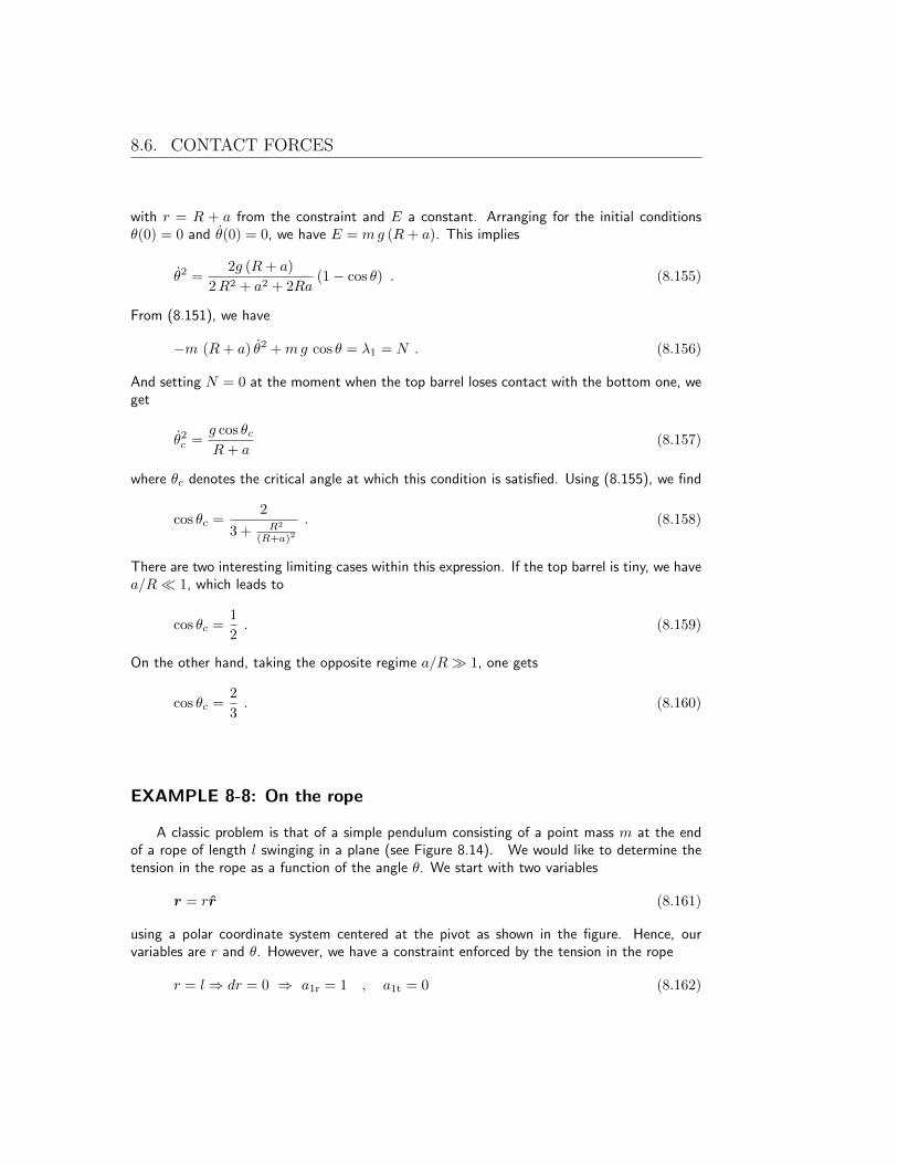
EXAMPLE 8-8: On the rope

A classic problem is that of a simple pendulum consisting of a point mass m at the endof a rope of length l swinging in a plane (see Figure 8.14). We would like to determine thetension in the rope as a function of the angle θ. We start with two variables

r = rr (8.161)

using a polar coordinate system centered at the pivot as shown in the figure. Hence, ourvariables are r and θ. However, we have a constraint enforced by the tension in the rope

r = l⇒ dr = 0 ⇒ a1r = 1 , a1t = 0 (8.162)


FIG 8.14 : A pendulum with a single constraint given by the fixed length of the rope.

which we immediately used to read off the relevant coefficients for (8.125). The kinetic energyis

T =1

2m(r2 + r2θ2

)(8.163)

while the potential energy is simply

V = −mgr cos θ . (8.164)

The Lagrangian becomes

L = T − V =1

2m(r2 + r2θ2

)+mgr cos θ (8.165)

where we keep track of both r and θ as independent degrees of freedom at the cost ofintroducing a single Lagrange multiplier λ1 associated with the constraint. The equation ofmotion for r comes from (8.124) and looks like

mr +mrθ2 −mg cos θ = λ1 = F · ∂r∂r

= Fr = T . (8.166)

While that for θ looks like

d

dt

(mr2θ

)+mgr sin θ = 0 . (8.167)

The three degrees of freedom are associated with three differential equations, where the thirdcomes of course from the constraint (8.162), which we now write as

r = 0 . (8.168)

8.6. CONTACT FORCES

This is sufficient to determine all three variables of interest. Once again, however, it is easierto use energy conservation

E = T + V =1

2ml2θ2 −mg l cos θ . (8.169)

We start with initial conditions

θ(0) = θ0 , θ(0) = 0 ⇒ E = −mg l cos θ0 . (8.170)

We then have

θ2 =2g

l(cos θ − cos θ0) . (8.171)

This allows us to find the Lagrange multiplier λ1 in terms of θ

λ1 = −mg cos θ + 2mg (cos θ − cos θ0) = −mg (cos θ − 2 cos θ0) = T , (8.172)

the tension in the rope.

CHAPTER 8

Problems

PROBLEM 8-1: Consider an infinite wire carrying a constant linear charge density λ0.Write the Lagrangian of a probe charge Q in the vicinity, and find its trajectory.

PROBLEM 8-2: Consider the oscillating Paul trap potential

U(z, r) =U0 + U1 cos Ωt

r20 + 2 z2

0

(2 z2 +

(r20 − r2

))(8.173)

written in cylindrical coordinates. (a) Show that this potential satisfies Laplace’s equation.(b) Consider a point particle of charge Q in this potential. Analyze the dynamics using aLagrangian and show that the particle is trapped.

PROBLEM 8-3: Show that the Coulomb gauge ∇ ·A = 0 is a consistent gauge condition.

PROBLEM 8-4: Find the residual gauge freedom in the Coulomb gauge.

PROBLEM 8-5: Show that the Lorentz gauge ∂µAνηµν = 0 is a consistent gauge condition.

PROBLEM 8-6: Find the residual gauge freedom in the Lorentz gauge.

PROBLEM 8-7: A particle of mass m slides inside a smooth hemispherical bowl of radiusR. Use spherical coordinates r, θ and ϕ to describe the dynamics. (a) Write the Lagrangianin generalized coordinates and solve the dynamics. (b) Repeat the exercise using a Lagrangemultiplier. What does the multiplier measure in this case?

PROBLEM 8-8: A pendulum consisting of a ball at the end of a rope swings back andforth in a two-dimensional vertical plane, with the angle θ between the rope and the verticalevolving in time. However, the rope is pulled upward at a constant rate so that the length lof the pendulum’s arm is decreasing as in dl/dt = −α ≡ constant. (a) Find the Lagrangianfor the system with respect to the angle θ. (b) Write the corresponding equations of motion.(c) Repeat parts (a) and (b) using Lagrange multipliers.

PROBLEM 8-9: A particle of mass m slides inside a smooth paraboloid of revolutionwhose surface is defined by z = αρ2, where z and ρ are cylindrical coordinates. (a) Write theLagrangian for the three dimensional system using the method of Lagrange multipliers. (b)Find the equations of motion.

PROBLEM 8-10: In certain situations, it is possible to incorporate frictional effects withoutintroducing the dissipation function. As an example, consider the Lagrangian

L = eγt(

1

2mq2 − 1

2kq2

). (8.174)

PROBLEMS

(a) Find the equation of motion for the system. (b) Do a coordinate change s = eγt/2q.Rewrite the dynamics in terms of s. (c) How would you describe the system?

PROBLEM 8-11: A massive particle moves under the acceleration of gravity and withoutfriction on the surface of an inverted cone of revolution with half angle α. (a) Find theLagrangian in polar coordinates. (b) Provide a complete analysis of the trajectory problem,mimicking what we did for the case of Newtonian potential in class. Do not integrate the finalorbit equation, but explore circular orbits in detail. (c) Repeat using Lagrange multipliers.

PROBLEM 8-12: A toy model for our expanding universe during the inflationary epochconsists of a circle of radius r(t) = r0e

ωt with our miserable lives confined on the one-dimensional world that is the circle. To probe the physics, imagine two point masses ofidentical mass m free to move on this circle without friction, connected by a spring of springconstant k and relaxed length zero, as depicted in the figure. (a) Write the Lagrangian for thetwo-particle system in terms of the common radial coordinate r and the two polar coordinatesθ1 and θ2. Do NOT implement the radial constraint r(t) = r0e

ωt yet. (b) Using a Lagrangemultiplier for the radial constraint, write four equations describing the dynamics. In process,you better show that

a1r = 1 , a1t = −ωr . (8.175)

(c) Consider the coordinate relabeling

α ≡ θ1 + θ2 , β ≡ θ1 − θ2 . (8.176)

Show that the equations of motion of part (b) for the two angle variables θ1 and θ2 can berewritten in a decoupled form as

α = C1α ; (8.177)

β = C2β + C3β ; (8.178)

where C1, C2 and C3 are constants that you will need to find.

PROBLEM 8-13: For the previous problem, (a) identify a symmetry transformation δt, δα, δβfor this system. Find the associated conserved quantity. What would you call this conservedquantity? (b) Then find α(t) and β(t) using equations (8.177) and (8.178). Use the boundaryconditions:

α(0) = α0 , α(0) = 0 , β(0) = 0 , β(0) = C , (8.179)

What is the effect of the expansion on the dynamics? NOTE: This conclusion is the same as inthe more realistic three dimensional cosmological scenario! (c) Find the force on the particlesexerted by the expansion of the universe. Write this as a function of α(t), β(t), and r(t); andthen show that its limiting form for later times in the evolution is given by

2mω2 r(t) . (8.180)

CHAPTER 8

k

k'

!

m

r

R

θ

Θ

PROBLEM 8-14:

The figure above shows a mass m connected to a spring of spring constant k along awooden track. The mass is restricted to move along this track without friction. The wholesetup is mounted on a toy wagon of zero mass resting on a track along a second frictionlessbeam. The wagon is connected by a spring of spring constant k′ to an axle about which thewhole darn thing is spinning with constant angular speed ω. The figure is a top-down view, withgravity pointing into the page, and the rest length of each spring is zero. Take a deep breathwhile reciting the Latin alphabet backwards. (a) First, write the Lagrangian of the system interms of the four variables r, θ, R, and Θ shown on the Figure, without implementing anyconstraints. (b) Identify two constraint equations. Implement the one keeping the two tracksperpendicular to each other into the result of part (a) by eliminating R. Do NOT implementthe one that spins things at constant angular speed ω. (c) Introducing a Lagrange multiplierfor the constraint having to do with the spin, write four differential equations describing thesystem. (d) Identify the force on the mass m due to the spin of the setup, and find allconditions for which this force vanishes!

PROBLEM 8-15: Consider the system shown in the figure below. The particle of massm2 moves on a vertical axis without friction and the whole contraption rotates about this axiswith a constant angular speed Ω. The frictionless joint near the top assures that the threemasses always lie in the same plane; and the rods of length a are all rigid. (HINT: Use theorigin of your coordinate system at the upper frictionless joint.) (a) Find the equation ofmotion in terms of one degree of freedom θ. (b) Using the method of Lagrange multipliers,find the torque on the masses m1 due to the rotational motion. (c) Find a static solution

PROBLEMS

a

a

a

a

m1m1

m2

frictionless joint!

!

in θ and identify the corresponding angle in terms of m1, m2, g, a, and Ω. Consider somelimits/inequalities in your result and comment on whether they make sense. (d) Is the solutionin part (c) stable? if so, what is the frequency of small oscillations about the configuration.(HINT: Use ξ = cos θ and work on the Lagrangian instead of the equation of motion.)

CHAPTER 8

james clerk maxwell (1831 - 1879)saeta.physics.hmc.edu/courses/p111/uploads/y2012/ch08.pdfjames...

Documents