jamye curry b,1 b abstract. manuscript - imstat.org · abstract. we study a rank based univariate...

BJPS - A

ccep

ted M

anusc

ript

Submitted to the Brazilian Journal of Probability and Statistics

A rank-based Cramer-von-Mises-type test for twosamples

Jamye Currya, Xin Dangb,1 and Hailin Sangb

aGeorgia Gwinnett CollegebUniversity of Mississippi

Abstract. We study a rank based univariate two-sample distribution-free test. The test statistic is the difference between the average ofbetween-group rank distances and the average of within-group rank dis-tances. This test statistic is closely related to the two-sample Cramer-von Mises criterion. They are different empirical versions of a same quan-tity for testing the equality of two population distributions. Althoughthey may be different for finite samples, they share the same expectedvalue, variance and asymptotic properties. The advantage of the newrank based test over the classical one is its ease to generalize to themultivariate case. Rather than using the empirical process approach, weprovide a different easier proof, bringing in a different perspective andinsight. In particular, we apply the Hajek projection and orthogonal de-composition technique in deriving the asymptotics of the proposed rankbased statistic. A numerical study compares power performance of therank formulation test with other commonly-used nonparametric testsand recommendations on those tests are provided.

1 Introduction

To test whether two samples come from the same or different populations,several distribution free tests such as the Kolmogorov-Smirnov test, theCramer-von Mises test and their variations have been proposed and widely

used. Let X1, X2, ..., Xmiid∼ F and Y1, Y2, ..., Yn

iid∼ G be two independentrandom samples with continuous distribution functions F and G, respec-tively. The two sample problem is to test

H0 : F = G vs Ha : F 6= G. (1)

Denote Fm and Gn as the empirical distribution functions of the two sam-ples and HN as the empirical distribution function of the combined sample,where N = m+n. The Kolmogorov-Smirnov (KS) two-sample test uses the

1Corresponding authorMSC 2010 subject classifications: 62G10, 62G20Keywords and phrases. Cramer-von Mises criterion, Hajek projection, nonparametric

test, rank, two-sample test

1imsart-bjps ver. 2014/10/16 file: "V1_Rank two sample test_BJPS".tex date: December 4, 2017

BJPS - A

ccep

ted M

anusc

ript

2

maximum distance (difference) between Fm and Gn. The classical Cramer-von Mises test statistic has the form

Tc =mn

N

∫ ∞−∞

[Fm(x)−Gn(x)]2dHN (x). (2)

This test statistic and its asymptotics have been well studied in the litera-ture, for example, Lehmann [22], Rosenblatt [27], Darling [9], Fisz [14] andAnderson [2].

Both of the KS test statistic and the Cramer-von Mises test statistic areformulated based on the empirical distributions. Baringhaus and Franz [3]studied a test statistic based on the original data. That is

mn

N{ 1

mn

m∑i=1

n∑j=1

|Xi − Yj | −1

2m2

m∑i=1

m∑j=1

|Xi −Xj | −1

2n2

n∑i=1

n∑j=1

|Yi − Yj |}.

(3)

This test statistic (3) was motivated by a conjecture considering the dis-tances between points of two types (Morgenstern, [23]) and it has a directgeneralization to the multivariate case. However, it requires an assumptionon the first moment and it is not distribution free for the univariate case(Baringhaus and Franz, [3]). It is worth to note that the test statistic (3)falls in the unified framework on energy statistics studied by Szekely andRizzo [30]. Other similar tests include [13] and [16], although they are derivedunder different motivations. Fernandez, Gamerro, and Garcıa [13] developeda statistic based on the empirical characteristic functions of the observed ob-servations. The statistic uses a weighted integral of the difference betweenthe empirical characteristic function of the two samples. Gretton et al. [16]proposed a test based on a kernel method in which the testing procedureis defined as the maximum difference in expectations over functions evalu-ated on the two samples. All of those test statistics are of the form being adifference on a measure of between-group and within-group.

In this paper, we propose a new rank based test of the same form. Nev-ertheless, it overcomes the limitations of (3). It is formulated based on theranks of two samples with respect to the combined sample HN . DenoteR(y,H) as the standardized rank of the quantity y with respect to the dis-tribution H, i.e., R(y,H) = H(y). For testing the hypothesis (1), we use the

imsart-bjps ver. 2014/10/16 file: "V1_Rank two sample test_BJPS".tex date: December 4, 2017

BJPS - A

ccep

ted M

anusc

ript

A rank based two-sample test 3

following test statistic.

T =mn

N{ 1

mn

m∑i=1

n∑j=1

|R(Xi, HN )−R(Yj , HN )|

− 1

2m2

m∑i=1

m∑j=1

|R(Xi, HN )−R(Xj , HN )|

− 1

2n2

n∑i=1

n∑j=1

|R(Yi, HN )−R(Yj , HN )|}. (4)

T is interpreted as the difference of the average of between-group rank dif-ferences and the average of within-group rank differences. A large value of Tindicates the deviation of two groups. The test based on T is distribution-freeand does not require any moment condition.

For the balanced samples (m = n), one can consider an equivalent butsimpler statistic

T ′ =1

mn

m∑i=1

n∑j=1

|R(Xi, HN )−R(Yj , HN )|. (5)

T ′ is the average of rank differences between two groups. T and T ′ areequivalent because T = nT ′ − (4n2 − 1)/(12n) when m = n.

As we will see later, the test statistic T is closely related to the classicalnonparametric Cramer-von Mises criterion Tc. They are different empiri-cal plug-in versions of the same population quantity. The rank based teststatistic and the Cramer-von Mises criterion may not be equal to each otherfor finite samples, but they are asymptotically equivalent. The advantageof the new rank based test over the classical one is its ease to generalizeto the multivariate case. Multivariate generalizations of Cramer-von Misestests have been considered by many researchers, but they are either appliedon independent data [8] or used for testing independence [15] or used inthe goodness-of-fit test of the uniform distribution on the transformed data[7]. For the rank based formulation, generalizations to the multivariate twosample problem are straightforward by applying notions of multivariate rankfunctions. In this paper, rather than using the empirical process approach,we provide a different easier proof, bringing in a different perspective andinsight. In particular, we apply the Hajek projection and orthogonal decom-position technique in deriving the asymptotics of the proposed statistic.

Some related works include Pettitt [26] and Baumgartner, Weiß, andSchindler [4]. They considered statistics of Anderson-Darling type that can


BJPS - A

ccep

ted M

anusc

ript

4

be viewed as standardized versions of Cramer-von Mises statistics. Schmidand Trede [28] utilized L1 Cramer-von Mises statistics. A rank-based repre-sentation of a L1 Cramer-von Mises statistic under a balanced size and itsgeneralizations are studied by Borroni [5]. Albers, Kallenberg and Martini [1]studied rank procedures for detecting shift alternatives with increasing shiftin the tail of the distribution. Janic-Wroblewska and Ledwina [21] considereda test based on a combination of several linear rank statistics. Related tothe rank procedures, other nonparametric tests include those based on theempirical likelihood approach. Einmahl and McKeague [12] considered teststatistics based on the empirical likelihood ratios for the goodness of fit andtwo sample problems. It has been proved that those tests are asymptoticallyequivalent to the one-sample and two sample Anderson-Darling tests. Caoand Van Keilegom [6] proposed an empirical likelihood ratio test via kerneldensity estimation. Gurevich and Vexler [17] utilized an empirical likelihoodratio test based on samples entropy.

The paper has the following structure. Section 2 presents the main results,including the formulation of the test statistic (4) and its properties. Thesimulation study is performed in Section 3. We summarize and conclude thepaper in Section 5. All proofs go to Section 6.

2 Main Results

To formulate the rank based test statistic T in (4), we first establish itspopulation version. We provide a result of the population version, from whichwe can see the relationship between our statistic and Cramer-von Misescriterion.

Theorem 2.1 Let X,X1, X2 and Y, Y1, Y2 be independent continuous ran-dom variables distributed from F and G, respectively. Let H = τF+(1−τ)Gwith 0 ≤ τ ≤ 1 be the mixture distribution. Then

E|R(X,H)−R(Y,H)|−1

2E|R(X1, H)−R(X2, H)|−1

2E|R(Y1, H)−R(Y2, H)| ≥ 0

(6)and the equality holds if and only if F = G.

The above result is based on the following identity which is obtained fromLemma 6.1 in the Appendix.

E|R(X,H)−R(Y,H)| − 1

2E|R(X1, H)−R(X2, H)| − 1

2E|R(Y1, H)−R(Y2, H)|

=

∫ ∞−∞

(F (x)−G(x))2d(τF (x) + (1− τ)G(x)). (7)


BJPS - A

ccep

ted M

anusc

ript


The result of Theorem 2.1 suggests two possible statistics for testing thehypothesis (1). The first version is the sample plug-in version of the left sideof (7). With τ = m/N and multiplying by mn/N , it is our test statistic de-fined in (4). H0 is rejected if the sample version is large, i.e., T > cα(m,n).The critical value cα(m,n) is determined by the significance level α andthe null distribution of T . The test statistic T is the difference of the aver-age of between-group rank differences and the average of within-group rankdifferences. A large value of T indicates the deviation of two groups.

The two-sample Cramer-von Mises statistic Tc in (2) is the empiricalversion of the right side of (7). Hence T and Tc are all plug-in statistics ofan equal quantity. Nevertheless, they may take different values. We shallthank one of the referees who pointed out this possibility. For example, inthe case that m = n = 2, let the two X realizations be 0 and 2 and thetwo Y realizations be 1 and 3. It is easy to see that the Cramer-von Misesstatistic has value 1

4 and the test statistic T has value 18 . Next, we will study

the properties of T .LetD be E|R(X,H)−R(Y,H)|−1

2E|R(X1, H)−R(X2, H)|−12E|R(Y1, H)−

R(Y2, H)|, and D = N/(mn)T . Then we have the following theorem.

Theorem 2.2 For m,n→∞, if m/(m+ n)→ τ , then D → D a.s.

By this theorem and Theorem 2.1, it is easy to see that our test statistic Tis consistent for the alternative Ha : F 6= G.

Theorem 2.3 Under H0, T is distribution free.

Under H0, the combined samples X1, ..., Xm, Y1, ..., Yn constitute a ran-dom sample of size N from the distribution F = G = H. So any assignmentof m numbers to X1, ..., Xm and n numbers to Y1, ..., Yn from the set of

integers {1, 2, ..., N} is equally likely, i.e. has probability

(N

m

)−1which is

independent of F . Using the fact that those number assignments have one-to-one linear relationship with the standardized ranks, T is distribution free.

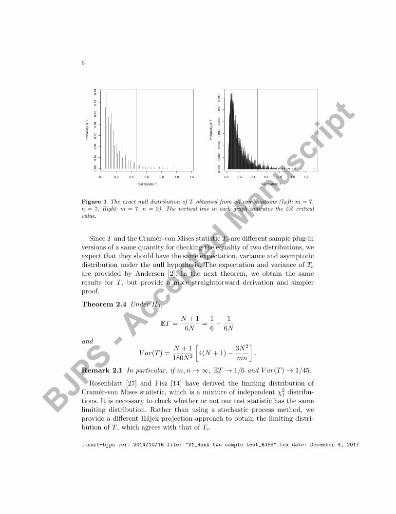
The exact null distribution of T can be found by enumeration of all possi-ble values of T by considering the N !/(m!n!) orderings of m X’s and n Y ’s.Figure 1 provides the exact null distribution of T for sample sizes m = n = 7and m = 7, n = 9 by considering all combinations. However, the exact nulldistribution is infeasible to obtain for large sample sizes because the numberof combinations increases dramatically as m and n increase. For large sam-ples, we can use Monte-Carlo method on all combinations to approximatethe null distribution. Also the limiting distribution of T can be used to de-termine the critical values of the test. Next we study asymptotic behaviorsof T .


BJPS - A

ccep

ted M

anusc

ript

6

0.0 0.2 0.4 0.6 0.8 1.0 1.2

0.0

00

.02

0.0

40

.06

0.0

80

.10

0.1

20

.14

Test Statistic T

Pro

ba

bili

ty o

f T

0.0 0.2 0.4 0.6 0.8 1.0 1.2

0.0

00

0.0

02

0.0

04

0.0

06

0.0

08

0.0

10

0.0

12

Test Statistic T

Pro

ba

bili

ty o

f T

Figure 1 The exact null distribution of T obtained from all combinations (Left: m = 7,n = 7; Right: m = 7, n = 9). The vertical line in each graph indicates the 5% criticalvalue.

Since T and the Cramer-von Mises statistic Tc are different sample plug-inversions of a same quantity for checking the equality of two distributions, weexpect that they should have the same expectation, variance and asymptoticdistribution under the null hypothesis. The expectation and variance of Tcare provided by Anderson [2]. In the next theorem, we obtain the sameresults for T , but provide a more straightforward derivation and simplerproof.

Theorem 2.4 Under H0,

ET =N + 1

6N=

1

6+

1

6N

and

V ar(T ) =N + 1

180N2

[4(N + 1)− 3N2

mn

].

Remark 2.1 In particular, if m,n→∞, ET → 1/6 and V ar(T )→ 1/45.

Rosenblatt [27] and Fisz [14] have derived the limiting distribution ofCramer-von Mises statistic, which is a mixture of independent χ2

1 distribu-tions. It is necessary to check whether or not our test statistic has the samelimiting distribution. Rather than using a stochastic process method, weprovide a different Hajek projection approach to obtain the limiting distri-bution of T , which agrees with that of Tc.


BJPS - A

ccep

ted M

anusc

ript


We obtain the first order Hajek projection T in Lemma 6.2 as

T =m∑i=1

E[T |Xi] +n∑j=1

E[T |Yj ]− (N − 1)ET,

where E[T |X1] = 16(1 + n

mN ) + 1N (1 − n

m)[F (X1) − F 2(X1)]. Under H0, Thas variance

V ar(T ) =

m∑i=1

V ar(E[T |Xi]) +

n∑j=1

V ar(E[T |Yj ])

=

[m(m− n)2

m2N2+n(m− n)2

n2N2

]V ar[F (Y1)− F 2(Y1)]

=(m− n)2

180mnN.

Clearly, V ar(T )/V ar(T )→ 0 as m,n→∞. Therefore the first order Hajekprojection is not sufficient in deriving the asymptotics of the statistic T .

To derive the asymptotics of the statistic T under the null hypothesis, itis necessary to have the second order projection T of T .

T =

m∑i=1

n∑j=1

E[T |Xi, Yj ] +∑

1≤i<j≤mE[T |Xi, Xj ]

+∑

1≤i<j≤nE[T |Yi, Yj ]−

N(N − 1)

2ET.

Since

E{E[T |X1, Y1]} = E{E[T |X1, X2]} = E{E[T |Y1, Y2]} = ET,

ET = 0. By Lemma 6.3 and Lemma 6.4, it can be examined that

Cov(E[T |Z1, Z2],E[T |Z1, Z3]) = 0,

where Z1, Z2 and Z3 are three different variables from Xi, Yj , 1 ≤ i ≤ m, 1 ≤j ≤ n, and

V ar(T ) =m4 + n4 − 2m3n− 2mn3 + 10m2n2 − 8mnN + 5n2 + 5m2

180N2mn

+m(m− 1)

2

m2 − 2mn+ 5n2

90m2N2+n(n− 1)

2

n2 − 2mn+ 5m2

90n2N2

=N2

180mn+

2

45N− N − 1

36mn− 1

18N2.


BJPS - A

ccep

ted M

anusc

ript

8

Then V ar(T )V ar(T ) → 1 as N → ∞ under the condition limN→∞m/n = 1. We

shall always assume this condition in the following analysis.Efron and Stein [11] discussed a general orthogonal decomposition of a

statistic. Here, our statistic T is decomposed as T + T + RN , where T isthe first order projection and RN is a negligible term. Hence the limitingdistribution of T is determined by the limiting distribution of T .

To determine the limiting distribution of T underH0, let h(x, y) = |F (x)−F (y)|+F (x)[1−F (x)] +F (y)[1−F (y)]− 2/3. Then h(x, y) is a degeneratekernel function since h(x, y) is symmetric and Eh(X, y) = 0. By Lemma

6.3 and Lemma 6.4, we have T =ˆT + R′N with V ar(R′N )/V ar(T ) → 0 as

N →∞ 1 and

ˆT =

1

N

m∑i=1

n∑j=1

h(Xi, Yj)−1

N

∑1≤i<j≤m

h(Xi, Xj)−1

N

∑1≤i<j≤n

h(Yi, Yj).

It is not difficult to verify that

V ar[h(Z1, Z2)] = 2/45 (8)

and Cov(h(Z1, Z2), h(Z1, Z3)) = 0, i.e., h(Z1, Z2) and h(Z1, Z3) are or-thogonal, where Z1, Z2 and Z3 are three different variables from Xi, Yj ,1 ≤ i ≤ m, 1 ≤ j ≤ n.

Now we define an operator A on the function space L2(R, F ) by

Ag∗(x) =

∫ ∞−∞

h(x, y)g∗(y)dF (y), x ∈ R, g∗ ∈ L2(R, F ).

This operator only has real eigenvalues since the kernel h(x, y) is symmetric.Let λ = λ1, λ2, · · · be the non-zero eigenvalues of the operator A obtainedby solving the equation Ag∗ = λg∗. With the substitution of u = F (x) andv = F (y), solving Ag∗ = λg∗ is equivalent to solve that∫ 1

0

{|u− v|+ u(1− u) + v(1− v)− 2

3

}g(v)dv = λg(u), (9)

where g = g∗ ◦ F−1. Taking the twice derivative with respect to u on bothsides of (9), we have the equation 2g(u) = λg′′(u). Solving it and substitut-ing back, we have the eigenvalues of A being λk = − 2

π2k2, k ∈ N and the

corresponding eigenfunctions φk(x) = cos(kπF (x)), k ∈ N. The eigenfunc-tion for the zero eigenvalue is φ0(x) = 1. Note that the eigenvalues do not

1If m = n→ ∞, R′N = 0.


BJPS - A

ccep

ted M

anusc

ript


depend on F , but the eigenfunctions {φk(x)}∞k=0 depend on F , which give a

orthonormal basis for the space L2(R, F ). Let TN =ˆT/√V ar(T ). Then we

have the following theorem.

Theorem 2.5 Under H0 and the condition limN→∞m/n = 1,

TNd−→ Z∞ = −

√45

2

∞∑k=1

λk(χ21k − 1),

where χ211, χ

212 · · · are independent χ2

1 variables and λk = − 2π2k2

, k ∈ N.Hence

(T − ET )/√V ar(T )

d−→ Z∞ = −√

45

2

∞∑k=1

λk(χ21k − 1)

since (T − ET − ˆT )/

√V ar(T )→ 0 in probability.

As expected, this asymptotical result agrees with the one for Cramer-vonMises statistic as proved with a stochastic process method in Rosenblatt[27] and Fisz [14]. This different projection approach we applied here istypically useful in U-statistic theory, but we shall emphasize that T is notan U-statistic.

d = 1 d = 2 d = 4 d = 10 d = 100

Variance ratio 0.9239 0.9819 0.9967 0.9997 1.000095% quantile 1.9298 1.9676 1.9772 1.9779 1.9780

Approximated cα(m,n) of T (α = 0.05) based on Zdm = n = 50 0.4545 0.4601 0.4617 0.4617 0.4617m = 50, n = 40 0.4545 0.4601 0.4615 0.4616 0.4616m = n = 500 0.4544 0.4600 0.4614 0.4615 0.4615m = n = 7 0.4543 0.4597 0.4610 0.4611 0.4611m = 7, n = 9 0.4540 0.4594 0.4608 0.4609 0.4609

Table 1 First part: variance ratios of Zd over Z∞ and 95% quantiles of Zd. Secondpart: approximated critical values for T . Comparing with the exact α = 0.049 critical

value 0.4643 for the case of m = n = 7 and the exact α = 0.05 critical value 0.4678 forthe case of m = 7, n = 9, the approximations are pretty accurate even under small sizes.

In practice, d = 4 or d = 10 is recommended.

In practice, we may approximate the limiting distribution by a distribu-tion of a finite linear combination of d independent χ2

1 random variables,i.e.

Zd = −√

45

2

d∑k=1

λk(χ21k − 1) =

√45

π2

d∑k=1

1

k2(χ2

1k − 1).


BJPS - A

ccep

ted M

anusc

ript

10

The accuracy of approximation depends on the choice of d. Table 1 providesratios of variance of the d mixture and that of the infinite mixture, that is,σ2(Zd)/σ

2(Z∞). Also the table lists 95% quantiles of Zd which are estimatedby the average of 10 sample quantiles each on M = 108 random samples.Those quantile values can be used to approximate the critical values cα(m,n)of T , which are given by the second part of Table 1. As we will see that evenfor small sample sizes, the approximated critical values are pretty accurateand close to the exact true values. For the case of m = n = 7, the true sizeof the test is 0.056 if the approximated critical value 0.4611 is used. For thecase of m = 7 and n = 9, the true size of the test is 0.052 if 0.4609 is used.In summary, d = 4 or d = 10 is recommended for a compromise betweencomputation and accuracy.

∆ KS W ELR ELT CT DT T

0 0.040 0.050 0.057 0.050 0.050 0.051 0.0500.041 0.047 0.031 0.047 0.048 0.048 0.049

0.25 0.162 0.228 0.182 0.224 0.226 0.191 0.2170.160 0.208 0.119 0.196 0.203 0.171 0.198

0.5 0.534 0.681 0.578 0.670 0.671 0.582 0.6520.498 0.621 0.446 0.603 0.615 0.526 0.600

0.75 0.875 0.949 0.902 0.945 0.943 0.901 0.9360.851 0.926 0.829 0.919 0.922 0.871 0.912

1 0.988 0.998 0.994 0.997 0.998 0.991 0.9960.979 0.995 0.976 0.994 0.994 0.984 0.993

Table 2 Power performance of each test with significance level α = 0.05 for the normaldistribution with location alternatives. Row 1: n = m = 50, Row 2: n = 50,m = 40

3 Simulations

By the simulation study in this section we demonstrate the performance ofthe T test. There are many nonparametric tests available for the two sampleproblem. It is by no means to conduct a comprehensive comparison. Herewe include Kolmogorov-Smirnov test (KS), Wilcoxon rank sum test (W)or Mood test (M), the empirical likelihood ratio test (ELR) proposed byGurevich anf Vexler [17], the empirical likelihood test (ELT) proposed byEinmahl and McKeague [12], Baringhaus and Franz’s Cramer test (CT), thetest studied in Fernandes et al. [13] (DT) in the study. It is necessary to notethat the CT and DT tests are not distribution-free tests, and their criticalvalues and p-values are based Monte-Carlo method on permutations in eachsample, which is implemented in the R package “cramer”. The R package


BJPS - A

ccep

ted M

anusc

ript


“dbEmpLikeGOF” is used for the ELR test in which the parameter is setto be 0.1 as suggested in [17]. The critical values of the ELT and our T testare computed through 107 random combinations on {1, ..., N}.

Various alternative distributions are considered. For each case,M = 10000iterations are computed to estimate powers by calculating the fraction of p-values less than or equal to α = 0.05 the level of significance. The MonteCarlo errors can be estimated by ±1.96

√p(1− p)/M . In particular, the size

of tests shall maintain in the interval (0.046, 0.054).


0 0.036 0.048 0.052 0.048 0.049 0.046 0.0470.045 0.054 0.036 0.054 0.055 0.051 0.054

0.25 0.130 0.163 0.124 0.160 0.158 0.142 0.1650.135 0.157 0.084 0.152 0.154 0.137 0.162

0.5 0.422 0.488 0.367 0.486 0.481 0.434 0.5010.402 0.449 0.268 0.440 0.439 0.394 0.462

0.75 0.776 0.830 0.710 0.825 0.818 0.783 0.8360.741 0.786 0.586 0.780 0.776 0.734 0.799

1 0.947 0.966 0.917 0.966 0.965 0.950 0.9710.929 0.946 0.842 0.946 0.944 0.925 0.954

Table 3 Power performance of each test with significance level α = 0.05 for the t3 withlocation alternatives. Row 1: n = m = 50, Row 2: n = 50,m = 40.

Table 2 shows the size and power performance for each test under thenormal distributions, where X1,. . . ,Xn ∼ N(0, 1) and Y1,. . . ,Ym ∼ N(∆, 1)with ∆ = 0, 0.25, 0.5, 0.75, and 1. When ∆ = 0, the KS test is undersized forboth the equal and unequal sample sizes cases; the ELR test is oversized inthe equal sample size case and seriously undersized for the sample unequalsize case; all other tests keep a desirable size. As expected, the W test is thebest among all tests since it is well-known to be powerful for the two-sampleproblem with a constant shift in location, especially when data follow logisticor normal distributions. The CT and ELT tests are comparable to W. TheT test is more powerful than the DT, KS and ELR tests. In the unequalsample size case, the W test is the best followed by the CT test. The ELTand T tests are comparable and significantly better than the DT, KS andELR tests.

The experiment is repeated for the t-distribution with 3 degrees of freedomand the result is presented in Table 3. Although the statistical power of the Ttest is the highest among all tests for all cases, its power differences with theW test or the ELT test are small so that those three tests are comparable.

Table 4 shows the power performance for the Pareto distribution, where


BJPS - A

ccep

ted M

anusc

ript

12


0 0.040 0.052 0.058 0.051 0.052 0.050 0.0510.044 0.050 0.032 0.050 0.050 0.053 0.052

0.25 0.417 0.443 0.906 0.599 0.205 0.287 0.4720.377 0.405 0.815 0.516 0.186 0.265 0.428

0.5 0.960 0.886 0.999 0.978 0.655 0.843 0.9680.940 0.859 0.998 0.958 0.598 0.798 0.948

0.75 0.999 0.989 1.000 0.999 0.945 0.993 0.9990.998 0.980 1.000 0.998 0.908 0.988 0.997

1 1.000 0.999 1.000 1.000 0.993 1.000 1.0001.000 0.998 1.000 1.000 0.988 1.000 1.000

Table 4 Power performance of each test with significance level α = 0.05 for the Paretodistributions with location alternatives. Row 1: n = m = 50, Row 2: n = 50,m = 40.

X1,. . . ,Xn ∼ Pa(2, 2) and Y1,. . . ,Ym ∼ Pa(2+∆, 2) are generated, with ∆ =0, 0.25, 0.5, 0.75, and 1. The power of the ELR test is much higher thanthat of all others. For ∆ = 0.25, the power of the ELR test is as high as90%, which is 30% higher than the second best ELT test. The T test is thethird best one. The power difference between the T test and that of the CTtest can be as large as 27% for equal sample sizes and can be as large as32% for unequal sample sizes.

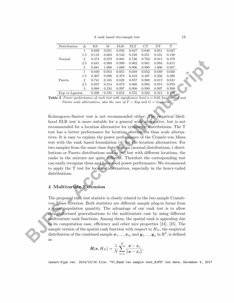
All considered tests as in the experiment for location alternatives areused for scale alternatives except the Wilcoxon test (W), as this is a test forlocation. Instead, the Mood’s test known as a scale test is used and referredto as the M test. Table 5 displays the results when Y samples of size 50 aregenerated from N(0,∆) or Pareto(2, 2∆), where ∆ = 1, 1.5, 2, 2.5, and 3. Inthe normal case, the T test does not compare favorably to all considered testsother than the KS test. It performs significantly better than the KS test,but its power is 2-5 times smaller than that of others. It is interesting to seethat the M test outperforms all tests in the normal case but it is the inferiorin the Pareto case. The T test has better performance for Pareto samplesthan for normal samples due to the heavy tails in Pareto distributions. Inthe Pareto case, all tests outperform the M test by a great margin and theCT test is the superior. As suggested by a reviewer, we add one more case inthe simulation in which X1, ..., Xn ∼ exp(1) and Y1, ..., Ym ∼ lognorm(0, 1)with sample sizes m = n = 50. The Monte Carlo powers of the seven testsare listed in Table 5. In this scenario, the T test performs better than KSand DT, but does not compare as favorably to the CT, W, ELT and ELRtests.

In general, the T test is not recommended for scale alternatives. The


BJPS - A

ccep

ted M

anusc

ript


Distribution ∆ KS M ELR ELT CT DT T

1 0.039 0.051 0.056 0.047 0.049 0.051 0.0471.5 0.118 0.663 0.542 0.238 0.251 0.431 0.138

Normal 2 0.374 0.979 0.965 0.746 0.792 0.915 0.4792.5 0.681 0.999 0.999 0.962 0.981 0.994 0.8153 0.881 1.000 1.000 0.996 0.999 1.000 0.957

1 0.040 0.054 0.055 0.049 0.052 0.049 0.0501.5 0.307 0.098 0.378 0.418 0.487 0.356 0.398

Pareto 2 0.741 0.165 0.828 0.857 0.909 0.815 0.8312.5 0.937 0.214 0.973 0.980 0.992 0.974 0.9783 0.988 0.234 0.997 0.998 0.999 0.997 0.998

Exp vs Lgnorm 0.336 0.535 0.654 0.555 0.502 0.315 0.476

Table 5 Power performance of each test with significance level α = 0.05 for Normal andPareto scale alternatives, also the case of F = Exp and G = Lognorm.

Kolmogorov-Smirov test is not recommended either. The empirical likeli-hood ELR test is more suitable for a general scale alternative, but is notrecommended for a location alternative for symmetric distributions. The Ttest has a better performance for location alternatives than scale alterna-tives. It is easy to explain the power performance of the Cramer-von Misestest with the rank based formulation (4) for the location alternatives. Fortwo samples from the same class distributions (normal distributions, t distri-butions or Pareto distributions and so on) but with different locations, theranks in the mixture are quite different. Therefore the corresponding testcan easily recognize them and have good power performance. We recommendto apply the T test for location alternatives, especially in the heavy-taileddistributions.

4 Multivariate Extension

The proposed rank test statistic is closely related to the two sample Cramer-von Mises criterion. Both statistics are different sample plug-in forms froma same population quantity. The advantage of our rank test is to allowstraightforward generalizations to the multivariate case by using differentmultivariate rank functions. Among them, the spatial rank is appealing dueto its computation ease, efficiency and other nice properties [24], [25]. Thesample version of the spatial rank function with respect to HN , the empiricaldistribution of the combined sample x1, ...,xm and y1, ...,yn in Rd, is definedas

R(x, HN ) =1

N

N∑i=1

x− zi‖x− zi‖

,


BJPS - A

ccep

ted M

anusc

ript

14

where zi = xi for i = 1, ...,m, zm+i = yi for i = 1, ..., n and ‖ · ‖ is theEuclidian distance. Then the multivariate two-sample spatial rank statistic,denoted by TM , is defined as

TM =mn

N{ 1

mn

m∑i=1

n∑j=1

‖R(xi, HN )−R(yj , HN )‖

− 1

2m2

m∑i=1

m∑j=1

‖R(xi, HN )−R(xj , HN )‖

− 1

2n2

n∑i=1

n∑j=1

‖R(yi, HN )−R(yj , HN )‖}. (10)

The test statistic TM is the difference of the average of the intra-group rankdistances and the average of the inter-group rank distances. A large value ofTM indicates the deviation of the two groups and rejects the null hypothesis.The multivariate counterpart of Theorem 2.1 states as follows.

Theorem 4.1 LetX,X1,X2 and Y ,Y 1,Y 2 be independent d-variate con-tinuous random vectors distributed from F and G, respectively. Let H =τF + (1− τ)G with 0 ≤ τ ≤ 1. Then

E‖R(X, H)−R(Y , H)‖ − 1

2E‖R(X1, H)−R(X2, H)‖

− 1

2E‖R(Y 1, H)−R(Y 2, H)‖ ≥ 0, (11)

where the equality holds if and only if F = G.

The multivariate spatial rank test based on TM loses the distribution-free property under the null hypothesis. The test relies on the permutationmethod to determine critical values or compute p-values. But the test isrobust. For example, it does not require the assumption of finite secondmoment as the Hotelling’s T 2 test. Neither it requires the assumption offinite first moment as the test (CT) considered by Baringhaus and Franz[3].

A simulation is conducted to compare performance of TM , CT and theHotelling’s T 2 under multivariate normal, t1 and Pareto distributions on Rd(d = 2, 5). Location and scatter alternatives are considered. For locationalternatives in normal and t1 distributions, the parameters of distributionsfor generating X samples of size n = 50 are µ = 0 and ΣX = I, whilefor Y samples with size m = 50 are µ = (∆, ...,∆)T and ΣY = I, where∆ = 0, 0.25, 0.5, 0.75 and 1. For Pareto distribution, X = (X1, ..., Xd)

T is


BJPS - A

ccep

ted M

anusc

ript


generated with each component Xj from Pareto(1,1) and Y = (Y1, ..., Yd)T

is generated with each component Yj from Pareto(1 + ∆, 1). R package“Hotelling” is used for the Hotelling’s T 2 test. TM and CT tests use thepermutation method to compute p-values and M = 10000 iterations arecomputed to estimate powers by calculating the fraction of p-values lessthan or equal 0.05. Results for the location alternatives are listed in Table6.

Dist Dim Method ∆ = 0 ∆ = .25 ∆ = .50 ∆ = .75 ∆ = 1

TM 0.0550 0.3000 0.8688 0.9966 1d = 2 CT 0.0556 0.3090 0.8818 0.9972 1

Hotelling 0.0518 0.3226 0.8900 0.9976 1Norm TM 0.0484 0.5178 0.9944 1 1

d = 5 CT 0.0500 0.5332 0.9958 1 1Hotelling 0.0494 0.5248 0.9942 1 1

TM 0.0538 0.1574 0.4898 0.8212 0.9644d = 2 CT 0.0596 0.0820 0.226 0.4504 0.7134

Hotelling 0.0546 0.0562 0.0934 0.136 0.2058t1 TM 0.0478 0.2382 0.7986 0.9888 0.9996

d = 5 CT 0.0546 0.0858 0.288 0.6200 0.8568Hotelling 0.0472 0.0742 0.1622 0.299 0.4608

TM 0.0492 0.3470 0.8682 0.9886 0.9998d = 2 CT 0.0560 0.1146 0.2850 0.5330 0.7298

Hotelling 0.0484 0.0986 0.1858 0.3076 0.4188Pareto TM 0.0522 0.2892 0.7942 0.9784 0.9996

d = 5 CT 0.0492 0.1142 0.2942 0.5184 0.7128Hotelling 0.0528 0.1108 0.2614 0.4462 0.6046

Table 6 Power performance of TM , CT and Hotelling tests with significance levelα = 0.05 for multivariate normal, t1 and Pareto distributions with location alternatives

with sample sizes n = m = 50.

From Table 6, three tests keep the size 5% well. Powers in d = 5 arehigher than that in d = 2 for each of three tests under all distributions. Inthe normal cases, TM performs slightly worse than the Hotelling’s test andCT. The power of TM is about 2% lower than that of the Hotelling testand 1% lower than that of CT under Ha when ∆ = 0.25 and ∆ = 0.50.However, the power gain of TM over CT and the Hotelling’s test is huge inthe t1-distributions. For ∆ = 0.25 and ∆ = 0.5, TM is about twice powerfulas CT and about triple powerful as the Hotelling test. The advantage ofour proposed TM over CT and the Hotelling’s test are even more significantin the asymmetric Parato distributions than in the t1 distributions for thelocation alternatives.

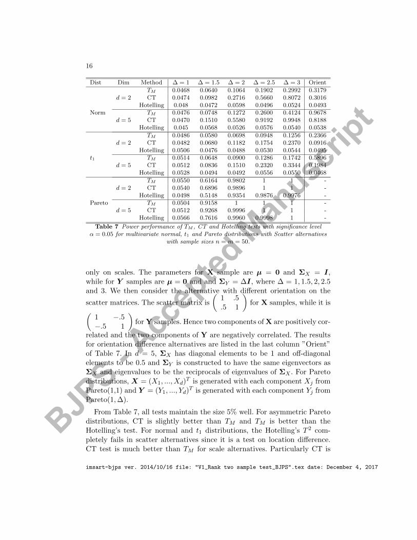
Results for scatter alternatives are listed in Table 7. For multivariate nor-mal and t1 distributions, we first consider the difference of scatter matrix


BJPS - A

ccep

ted M

anusc

ript

16

Dist Dim Method ∆ = 1 ∆ = 1.5 ∆ = 2 ∆ = 2.5 ∆ = 3 Orient

TM 0.0468 0.0640 0.1064 0.1902 0.2992 0.3179d = 2 CT 0.0474 0.0982 0.2716 0.5660 0.8072 0.3016

Hotelling 0.048 0.0472 0.0598 0.0496 0.0524 0.0493Norm TM 0.0476 0.0748 0.1272 0.2600 0.4124 0.9678

d = 5 CT 0.0470 0.1510 0.5580 0.9192 0.9948 0.8188Hotelling 0.045 0.0568 0.0526 0.0576 0.0540 0.0538

TM 0.0486 0.0580 0.0698 0.0948 0.1256 0.2366d = 2 CT 0.0482 0.0680 0.1182 0.1754 0.2370 0.0916

Hotelling 0.0506 0.0476 0.0488 0.0530 0.0544 0.0495t1 TM 0.0514 0.0648 0.0900 0.1286 0.1742 0.5896

d = 5 CT 0.0512 0.0836 0.1510 0.2320 0.3344 0.1984Hotelling 0.0528 0.0494 0.0492 0.0556 0.0550 0.0468

TM 0.0550 0.6164 0.9802 1 1 -d = 2 CT 0.0540 0.6896 0.9896 1 1 -

Hotelling 0.0498 0.5148 0.9354 0.9876 0.9976 -Pareto TM 0.0504 0.9158 1 1 1 -

d = 5 CT 0.0512 0.9268 0.9996 1 1 -Hotelling 0.0566 0.7616 0.9960 0.9998 1 -

Table 7 Power performance of TM , CT and Hotelling tests with significance levelα = 0.05 for multivariate normal, t1 and Pareto distributions with Scatter alternatives

with sample sizes n = m = 50.

only on scales. The parameters for X sample are µ = 0 and ΣX = I,while for Y samples are µ = 0 and and ΣY = ∆I, where ∆ = 1, 1.5, 2, 2.5and 3. We then consider the alternative with different orientation on the

scatter matrices. The scatter matrix is

(1 .5.5 1

)for X samples, while it is(

1 −.5−.5 1

)for Y samples. Hence two components of X are positively cor-

related and the two components of Y are negatively correlated. The resultsfor orientation difference alternatives are listed in the last column ”Orient”of Table 7. In d = 5, ΣX has diagonal elements to be 1 and off-diagonalelements to be 0.5 and ΣY is constructed to have the same eigenvectors asΣX and eigenvalues to be the reciprocals of eigenvalues of ΣX . For Paretodistributions, X = (X1, ..., Xd)

T is generated with each component Xj fromPareto(1,1) and Y = (Y1, ..., Yd)

T is generated with each component Yj fromPareto(1,∆).

From Table 7, all tests maintain the size 5% well. For asymmetric Paretodistributions, CT is slightly better than TM and TM is better than theHotelling’s test. For normal and t1 distributions, the Hotelling’s T 2 com-pletely fails in scatter alternatives since it is a test on location difference.CT test is much better than TM for scale alternatives. Particularly CT is


BJPS - A

ccep

ted M

anusc

ript


triple powerful as the TM in normal case and twice powerful in the t1 case.This result is not surprising since TM is based on the spatial ranks that losemajor information on distances or scales. However, when two scatter ma-trices of distributions are different on orientation, TM performs better thanCT, especially in t1 distribution, the power of TM is twice or triple as thatof CT.

5 Summary

The problem of testing whether two samples come from the same or differ-ent population is a classical one in statistics. In this paper, we have studieda rank-based test for the univariate two sample problem. The test statis-tic is the difference between the average of between-group rank distancesand the average of within-group rank distances. Under the null hypothesis,it is distribution free. The limiting null distribution was explored throughtechniques of Hajek projection and orthogonal decomposition. It has beenproved that the limiting distribution is not normal since the projection onone variable is insufficient to represent the variation of the test statistic.By taking the second-order projection, an operator in the functional spacewas defined and its eigenfunctions and eigenvalues were applied to derivethe limiting distribution. It is a weighted mixture of independent chi-squaredistributions with the weights being the eigenvalues of the operator. Weprovided a recommendation how to use the limiting distribution to obtaincritical values of the proposed test in practice.

The proposed rank test statistic is closely related to two sample Cramer-von Mises criterion. Both statistics are different sample plug-in forms fromthe same population quantity. We have provided a counter example to showthey are different. However, they have the same expectation, variance andlimiting distribution. The advantage of our rank test is to allow straightfor-ward generalizations to the multivariate case by using different multivariaterank functions. A continuation of this work is to study properties of themultivariate Cramer-von Mises TM test. Also the generalizations based onother multivariate rank functions deserve further investigation.

6 Proofs

The following lemma gives the expected value of the absolute differencebetween the standardized ranks of X and Y .

Lemma 6.1 Let X and Y be independent continuous random variables fromF and G, respectively. Let H = τF +(1−τ)G with 0 ≤ τ ≤ 1 be the mixture


BJPS - A

ccep

ted M

anusc

ript

18

distribution, J be the distribution of R(X,H) and K be the distributionfunction of R(Y,H). Then

E|R(X,H)−R(Y,H)| =∫ 1

0J(t)(1−K(t)) dt+

∫ 1

0K(t)(1−J(t)) dt. (12)

Proof of Lemma 6.1. Notice that

|R(X,H)−R(Y,H)|

=

∫ 1

0[I(R(X,H) ≤ s < R(Y,H)) + I(R(Y,H) ≤ s < R(X,H))] ds.

Since H is continuous and R(X,H) = H(X), R(Y,H) = H(Y ), we haveJ(x) = F ◦H−1(x), K(x) = G ◦H−1(x) for any x ∈ [0, 1], where H−1(x) =inf{u : H(u) ≥ x}. Then (12) holds by Fubini’s Theorem. �

Proof of Theorem 2.2. Define

D =1

mn

m∑i=1

n∑j=1

|R(Xi, H)−R(Yj , H)|

− 1

2m2

m∑i=1

m∑j=1

|R(Xi, H)−R(Xj , H)|

− 1

2n2

n∑i=1

n∑j=1

|R(Yi, H)−R(Yj , H)|.

Conditioning on Yj , 1 ≤ j ≤ n, by the law of large numbers,

1

m

m∑i=1

|R(Xi, H)−R(Yj , H)| − EX1 |R(X1, H)−R(Yj , H)| → 0 a.s.,

and

1

mn

m∑i=1

n∑j=1

|R(Xi, H)−R(Yj , H)|

=1

n

n∑j=1

[EX1 |R(X1, H)−R(Yj , H)|+ oa.s.(1)]

= E|R(X,H)−R(Y,H)|+ oa.s.(1).


BJPS - A

ccep

ted M

anusc

ript


By the strong law of large numbers for U -statistics [20],

1

2m2

m∑i=1

m∑j=1

|R(Xi, H)−R(Xj , H)| → 1

2E|R(X1, H)−R(X2, H)| a.s.,

and

1

2n2

n∑i=1

n∑j=1

|R(Yi, H)−R(Yj , H)| → 1

2E|R(Y1, H)−R(Y2, H)| a.s.

Then D → D a.s. as m,n→∞. Now we show D − D → 0 a.s.By Glivenko-Cantelli theorem, for m/N → τ ,

R(x,HN )→ R(x,H) a.s.

uniformly on x ∈ R. Then

|R(x,HN )−R(y,HN )| → |R(x,H)−R(y,H)| a.s.

uniformly on x, y ∈ R and therefore,

D − D =1

mn

m∑i=1

n∑j=1

{|R(Xi, HN )−R(Yj , HN )| − |R(Xi, H)−R(Yj , H)|}

− 1

2m2

m∑i=1

m∑j=1

{|R(Xi, HN )−R(Xj , HN )| − |R(Xi, H)−R(Xj , H)|}

− 1

2n2

n∑i=1

n∑j=1

{|R(Yi, HN )−R(Yj , HN )| − |R(Yi, H)−R(Yj , H)|} .

→ 0 a.s.

This completes the proof. �

Since all sample ranks are computed with respect to the combined sample,for simple presentation, we write the standardized rank R(Xi, HN ) as R(Xi).We also denote the natural rank of Xi as Ri, that is, R(Xi) = Ri/N .

Proof of Theorem 2.4. Under H0, R(Xi) and R(Yj) are identically dis-tributed from the discrete uniform distribution on {1/N, 2/N, ..., (N−1)/N, 1}for all i’s and j’s. Hence

ET

=mn

N

{E|R(X1)−R(Y1)| −

m− 1

2mE|R(X1)−R(X2)| −

n− 1

2nE|R(Y1)−R(Y2)|

}=

1

2E|R(X1)−R(X2)| =

1

2NE|R1 −R2|,


BJPS - A

ccep

ted M

anusc

ript

20

where R1 and R2 are natural ranks of X1 and X2, respectively. Under H0,R1 and R2 are two samples drawn uniformly from {1, 2, ..., N} without re-placement. Clearly,

E|R1 −R2| =1

N(N − 1)

N∑i=1

N∑j=1

|i− j| = N + 1

3. (13)

Hence ET =N + 1

6N.

Let R1, R2, R3, R4 be natural ranks of X1, X2, X3 and X4, respectively.We have

E(R1 −R2)2 =

1

N(N − 1)

N∑i=1

N∑j=1

(i− j)2 =N(N + 1)

6, (14)

E|R1 −R2||R1 −R3| =1

N(N − 1)(N − 2)

N∑i=1

∑j 6=i

∑k 6=i,j

|i− j||i− k|

=1

N(N − 1)(N − 2)

N∑i=1

N∑j=1

∑k 6=j|i− j||i− k|

=(N + 1)(7N + 4)

60, (15)

and

E|R1 −R2||R3 −R4|

=1

N(N − 1)(N − 2)(N − 3)

N∑i=1

N∑j 6=i,j=1

N∑k 6=i,j,k=1

N∑l 6=i,j,k;l=1

|i− j||k − l|

=1

N(N − 1)(N − 2)(N − 3)

N∑i=1

N∑j=1

N∑k 6=i,j,k=1

N∑l 6=i,j,k;l=1

|i− j||k − l|

=(N + 1)(5N + 4)

45. (16)

Now extending T 2 and ET 2 yields the above three types of expectationsE(R1 − R2)

2, E|R1 − R2||R1 − R3| and E|R1 − R2||R3 − R4| denoted as


BJPS - A

ccep

ted M

anusc

ript


E1, E2, E3, respectively. That is,

ET 2 =m2n2

N4

{[mn

m2n2+

2m(m− 1)

4m2+

2n(n− 1)

4n4

]E1

+

[mn(m− 1)(n− 1)

m2n2+m(m− 1)(m− 2)(m− 3)

4m4+n(n− 1)(n− 2)(n− 3)

4n4

−2mn(m− 1)(m− 2)

2m3n− 2mn(n− 1)(n− 2)

2mn3+

2m(m− 1)n(n− 1)

4m2n2

]E3

+

[m2n2 −mn−mn(m− 1)(n− 1)

m2n2+

4m(m− 1)(m− 2)

4m4+

4n(n− 1)(n− 2)

4n4

−m2n(m− 1)−mn(m− 1)(m− 2)

m3n− mn2(n− 1)−mn(n− 1)(n− 2)

mn3

]E2

}=N + 1

60N2

[3N + 3− N2

mn

].

Hence,

V ar(T ) = ET 2 − (ET )2 =N + 1

180N2

[4(N + 1)− 3N2

mn

].

�

Lemma 6.2 Under H0, E[|R(X1) − R(X2)||X1] =1

2− N − 2

N[F (X1) −

F 2(X1)],

E[|R(X2)−R(X3)||X1] =1

3+

2

N[F (X1)− F 2(X1)] and hence

E(T |X1) =1

6

(1 +

n

mN

)+

1

N

(1− n

m

)[F (X1)− F 2(X1)].

Proof of Lemma 6.2. Let R1 be the natural rank of X1 and R2 be the nat-ural rank of X2. Under H0 and given X1, R1−1 has a binomial distributionwith parameters N − 1 and F (X1), that is,

P (R1−1 = u|X1) =

(N − 1

u

)F (X1)

u[1−F (X1)]N−1−u, u = 0, 1, ..., N−1.


BJPS - A

ccep

ted M

anusc

ript

22

Given R1, R2 is uniformly distributed from {1, 2, ..., N}/{R1}. So

E(|R1 −R2||X1)

=E[E(|R1 −R2||R1)|X1] =

N∑r1=1

1

N − 1

N∑i=1,6=r1

|r1 − i|

P (R1 = r1|X1)

=1

2(N − 1)

N∑r1=1

[(N − 1)N − 2(N − 1)(r1 − 1) + 2(r1 − 1)2]P (R1 = r1|X1)

=1

2N − (N − 1)F (X1) +

1

N − 1[(N − 1)F (X1)(1− F (X1) + (N − 1)2F 2(X1)]

=1

2N − (N − 2)[F (X1)− F 2(X1)].

Let R3 be the natural rank of X3. Under H0, we have

E(|R2 −R3||X1) = E[E(|R2 −R3||R1)|X1]

=N∑

r1=1

1

(N − 1)(N − 2)

N∑i=1,i6=r1

N∑j=1,j 6=i,r1

|i− j|

P (R1 = r1|X1)

=N(N + 1)

3(N − 2)− N − 2(N − 2)[F (X1)− F 2(X1)]

N − 2

=1

3N + 2[F (X1)− F 2(X1)].

It is clear that E(T |X1) contains the above conditional expectations E[|R(X1)−R(X2)||X1] and E[|R(X2)−R(X3)||X1] denoted as E∗1 and E∗2 , respectively.Then it follows that

E(T |X1)

=mn

N

{n

mnE∗1 +

mn− nmn

E∗2 −2(m− 1)

2m2E∗1 −

(m− 1)(m− 2)

2m2E∗2 −

n(n− 1)

2n2E∗2

}=mn

N

{1

m2(E∗1 − E∗2) +

N

2mnE∗2

}=

1

6

(1 +

n

mN

)+

1

N

(1− n

m

)[F (X1)− F 2(X1)].

This complete the proof. �

The following two lemmas are on the second order projection of T .


BJPS - A

ccep

ted M

anusc

ript


Lemma 6.3 Under H0, the second order projection of T on one X variableand one Y variable is

E[T |X1, Y1]

=mnN +N2 − 7mn

6mnN+

(2m− n)(n− 1)

mnNF (X1)[1− F (X1)]

+(2n−m)(m− 1)

mnNF (Y1)[1− F (Y1)]

+ I(Y1 > X1)

{5n−m6mnN

+m− 1

mNF (Y1)−

n− 1

nNF (X1)

}+ I(Y1 < X1)

{5m− n6mnN

− m− 1

mNF (Y1) +

n− 1

nNF (X1)

}(17)

and its variance is

V ar{E[T |X1, Y1]}

=m4 + n4 − 2m3n− 2mn3 + 10m2n2 − 8mnN + 5n2 + 5m2

180N2m2n2. (18)

Proof of Lemma 6.3. In the proof of next two lemmas, we use E[S|Z1, Z2, Z1 <Z2] to denote E[SI(Z1 < Z2)|Z1, Z2] for any random variables S, Z1 andZ2. Again, let Ri be the natural rank of Xi, i = 1, 2, 3, 4. Under H0 and givenX1 < X2, (R1, R2) has trinomial distribution with parameters F (X1), F (X2)−F (X1) and 1− F (X2), i.e.,

P (R1 = u,R2 = v|X1, X2, X1 < X2) (19)

=

(N − 2

u− 1, v − u− 1, N − v

)[F (X1)]

u−1 (20)

× [F (X2)− F (X1)]v−u−1[1− F (X2)]

N−vI(X1 < X2).

Therefore,

E[|R1−R2||X1, X2, X1 < X2] = {(N − 2)[F (X2)−F (X1)] + 1}I(X1 < X2).(21)

Under H0 and given R1, R2, the natural rank R3 of X3 has discrete uni-form distribution on the set {1, 2, · · · , N}/{R1, R2}, i.e.,

P (R3 = w|R1, R2) =1

N − 2


BJPS - A

ccep

ted M

anusc

ript

24

for 1 ≤ w ≤ N , w 6= R1, R2. Therefore,

E(|R1 −R3||X1, X2, X1 < X2)

= E[E(|R1 −R3||R1 < R2)|X1, X2, X1 < X2]

= E

1

N − 2

∑1≤i<R1

(R1 − i) +∑

R1<i≤N,i6=R2

(i−R1)

|X1, X2, X1 < X2

= E

(N2 +N − 2NR1 + 2R2

1 − 2R2

2(N − 2)|X1, X2, X1 < X2

)=

{N + 1

2− (N − 3)F (X1)[1− F (X1)]− F (X2)

}I(X1 < X2). (22)

The last equality (22) is from (19), the conditional distribution of (R1, R2).By a similar calculation,

E(|R1 −R3||X1, X2, X1 > X2)

=

{N − 1

2− (N − 3)F (X1)[1− F (X1)] + F (X2)

}I(X1 > X2). (23)

We also have

E(|R3 −R4||X1, X2, X1 < X2)

= E[E(|R3 −R4||R1 < R2)|X1, X2, X1 < X2]

= E

1

(N − 2)(N − 3)

∑1≤i,j≤N,i,j 6=R1,R2

|i− j||X1, X2, X1 < X2

=

{N − 1

3+ 2F (X1)[1− F (X1)] + 2F (X2)[1− F (X2)]

}I(X1 < X2).

(24)

Again, the last equality (24) is from (19), the conditional distribution of(R1, R2). Now let R1, R2 be the natural rank of X1 and Y1 respectively. R3

and R4 be the natural ranks of two other different Xi or Yj , 1 < i ≤ m, 1 <


BJPS - A

ccep

ted M

anusc

ript


j ≤ n. By the definition of T as in (4),

N

mnE[T |X1, Y1, X1 < Y1] =

1

mn{E[|R(X1)−R(Y1)||X1, Y1, X1 < Y1]

+ (n− 1)E(|R(X1)−R(Y2)||X1, Y1, X1 < Y1)

+ (m− 1)E(|R(X2)−R(Y1)||X1, Y1, X1 < Y1)

+ (m− 1)(n− 1)E(|R(X2)−R(Y2)||X1, Y1, X1 < Y1)}

− 1

2m2{2(m− 1)E(|R(X1)−R(X2)||X1, Y1, X1 < Y1)

+(m− 1)(m− 2)E(|R(X2)−R(X3)||X1, Y1, X1 < Y1)}

− 1

2n2{2(n− 1)E(|R(Y1)−R(Y2)||X1, Y1, X1 < Y1)

+(n− 1)(n− 2)E(|R(Y2)−R(Y3)||X1, Y1, X1 < Y1)}

=1

mnNE(|R1 −R2||X1, Y1, X1 < Y1)

+n−mm2nN

E(|R1 −R3||X1, Y1, X1 < Y1)

+m− nmn2N

E(|R2 −R3||X1, Y1, X1 < Y1)

+mnN + 6mn− 2N2

2m2n2NE(|R3 −R4||X1, Y1, X1 < Y1).

By (21), (22), (23) and (24), we have

E[T |X1, Y1, X1 < Y1] = I(Y1 > X1)

{1

N2{(N − 2)[F (Y1)− F (X1)] + 1}

+n−mmN2

{N + 1

2− (N − 3)F (X1)[1− F (X1)]− F (Y1)

}+m− nnN2

{N − 1

2− (N − 3)F (Y1)[1− F (Y1)] + F (X1)

}+mnN + 6mn− 2N2

2mnN2

{N − 1

3+ 2F (X1)[1− F (X1)] + 2F (Y1)[1− F (Y1)]

}}.

Hence

E[T |X1, Y1, X1 < Y1]

= I(Y1 > X1)

{mnN +N2 − 7mn+ 5n−m

6mnN

+(2m− n)(n− 1)

mnNF (X1)[1− F (X1)] +

(2n−m)(m− 1)

mnNF (Y1)[1− F (Y1)]

+m− 1

mNF (Y1)−

n− 1

nNF (X1)

}.


BJPS - A

ccep

ted M

anusc

ript

26

A similar calculation gives

E[T |X1, Y1, X1 > Y1]

= I(Y1 < X1)

{mnN +N2 − 7mn+ 5m− n

6mnN

+(2m− n)(n− 1)

mnNF (X1)[1− F (X1)] +

(2n−m)(m− 1)

mnNF (Y1)[1− F (Y1)]

−m− 1

mNF (Y1) +

n− 1

nNF (X1)

}.

Therefore (17) holds.

Let U1, U2 be i.i.d. uniform random variables on [0, 1], then

V ar{E[T |X1, Y1]

= V ar

{(2m− n)(n− 1)

mnNU1(1− U1) +

(2n−m)(m− 1)

mnNU2(1− U2)

+ I(U2 > U1)

{5n−m6mnN

+m− 1

mNU2 −

n− 1

nNU1

}+I(U2 < U1)

{5m− n6mnN

− m− 1

mNU2 +

n− 1

nNU1

}}.

Therefore (18) holds. This completes the proof. �

The following lemma gives the second order projection of T on two Xvariables or two Y variables.

Lemma 6.4 Under H0, the projection of T on two X variables is

E[T |X1, X2]

=n

N

{mN + 6n−m

6mn+m− 2n

mn[F (X1)(1− F (X1)) + F (X2)(1− F (X2))]

− 1

m|F (X2)− F (X1)|

}. (25)

The variance of the projection is

V ar{E[T |X1, X2]} =m2 − 2mn+ 5n2

90m2N2. (26)


BJPS - A

ccep

ted M

anusc

ript


The projection of T on two Y variables is

E[T |Y1, Y2]

=m

N

{nN + 6m− n

6mn+n− 2m

mn[F (Y1)(1− F (Y1)) + F (Y2)(1− F (Y2))]

− 1

n|F (Y2)− F (Y1)|

}.

The variance of the projections is

V ar{E[T |Y1, Y2]} =n2 − 2mn+ 5m2

90n2N2. (27)

Proof of Lemma 6.4. By symmetry, we only need prove the results for theprojection on two X variables. By the definition of T as in (4), under thenull hypothesis,

E[T |X1, X2, X1 < X2]

=mn

N

{2

m2NE[|R1 −R3||X1, X2, X1 < X2]

+2

m2NE[|R2 −R3||X1, X2, X1 < X2]

+mN − 6n

2m2nNE[|R3 −R4||X1, X2, X1 < X2]

− 1

m2NE[|R1 −R2||X1, X2, X1 < X2]

}.

By (21), (22), (23) and (24), we have

E[T |X1, X2, X1 < X2]

=n

N

{mN + 6n−m

6mn+m− 2n

mn[F (X1)(1− F (X1)) + F (X2)(1− F (X2))]

− 1

m[F (X2)− F (X1)]

}I(X1 < X2).

By symmetry, we have (25). Let U1, U2 be i.i.d. uniform random variableson [0, 1], then

V ar{E[T |X1, X2]}

=n2

N2V ar

{m− 2n

mn[U1(1− U1) + U2(1− U2)]−

1

m|U2 − U1|

}=m2 − 2mn+ 5n2

90m2N2.


BJPS - A

ccep

ted M

anusc

ript

28


In the following we provide a lemma which is useful in deriving the asymp-totics of the test statistic T .

Lemma 6.5 Let Sn(X1, X2, · · · , Xn) be a function of n independent ran-dom variables with decomposition Sn = Mn+Rn. If E(Rn) = Cov(Mn, Rn) =0 for any n and V ar(Sn)/V ar(Mn)→ 1 as n→∞, then |Rn|/

√V ar(Sn)→

0 in L2 norm and therefore |Rn|/√V ar(Sn)→ 0 in probability.

Proof of Lemma 6.5.

E[R2n/V ar(Sn)] =

E[(Sn − ESn)− (Mn − EMn)]2

V ar(Sn)

=V ar(Sn) + V ar(Mn)− 2E(Sn − ESn)(Mn − EMn)

V ar(Sn)

=V ar(Sn) + V ar(Mn)− 2E(Mn − EMn)2 − 2ERn(Mn − EMn)

V ar(Sn)

=V ar(Sn)− V ar(Mn)

V ar(Sn)= 1− V ar(Mn)/V ar(Sn)→ 0.

�

The above Lemma 6.5 is a result of Hajeck projection technique. See Hajekand Sidak [18] and Hettmansperger and McKean [19] for details.

Proof of Theorem 2.5. We can write h(x, y) =∑∞

k=1 λkφk(x)φk(y), where{φk(·)} are the orthonormal eigenfunctions corresponding to the eigenvalues{λk}, see Dunford and Schwartz [10], Serfling [29]. Since Eh(X, y) = 0 and

0 = V ar{E[h(X,Y )|Y ]} =∞∑k=1

λ2k(Eφk(X))2V ar(φk(Y )).

Therefore, E(φk(X)) = 0 for all k ≥ 1 and V ar[h(X,Y )] = Eh2(X,Y ) =∑∞k=1 λ

2k. By (8),

∞∑k=1

λ2k = V ar[h(X,Y )] = 2/45.

The above results can also be confirmed by λk = − 2π2k2

, φk(x) = cos kπF (x), k ∈N. DenoteWmk(X) = 1√

m

∑mi=1 φk(Xi),Wnk(Y ) = 1√

n

∑nj=1 φk(Yj), Zmk(X) =


BJPS - A

ccep

ted M

anusc

ript


1m

∑mi=1 φ

2k(Xi), Znk(Y ) = 1

n

∑nj=1 φ

2k(Yj). Define TNK by

√V ar(T )TNK =

1

N

m∑i=1

n∑j=1

K∑k=1

λkφk(Xi)φk(Yj)

− 1

N

∑1≤i<j≤m

K∑k=1

λkφk(Xi)φk(Xj)−1

N

∑1≤i<j≤n

K∑k=1

λkφk(Yi)φk(Yj).

Then

√V ar(T )TNK =

√mn

N

K∑k=1

λkWmk(X)Wnk(Y )

− m

N

K∑k=1

λk2

{W 2mk(X)− Zmk(X)

}− n

N

K∑k=1

λk2

{W 2nk(Y )− Znk(Y )

}.

(28)

Applying the argument as in Serfling [29], page 197, |EeixTN − EeixTNK | ≤|x|[E(TN − TNK)2]1/2]. It is easy to see that

E(TN − TNK)2 =

(mn

N2+m(m+ 1) + n(n− 1)

2N2

)1

V ar(T )

∞∑k=K+1

λ2k

= [45

2+ o(1)]

∞∑k=K+1

λ2k ≤ 23∞∑

k=K+1

λ2k.

For a given ε > 0 and fixed x, we can choose and fix K to be large enoughso that

|x|(23∞∑

k=K+1

λ2k)1/2 < ε.

Then we have |EeixTN − EeixTNK | < ε for all N . By (28), Theorem 2.4 andthe condition limN→∞

mn = 1, we may write

TNK =

√45

2

K∑k=1

λk{−[Wnk(X)−Wnk(Y )]2/2 + Znk(X)/2 + Znk(Y )/2

}+ rN .

It is easy to see that rN → 0 in probability. Let χ21k be iid χ2

1 random vari-

ables. Denote UK =√452

∑Kk=1 λk(−χ2

1k + 1) and U =√452

∑∞k=1 λk(−χ2

1k +1). Since EWmk(X) = EWnk(Y ) = 0 andWmk(X),Wnk(Y ) are orthonormal,then the random vector {(Wmk(X) −Wnk(Y ))/

√2}Kk=1 ⇒ N(0, IK×K) by


BJPS - A

ccep

ted M

anusc

ript

30

the Linderberg-Levy central limit theorem, Zmk(X) → 1 and Znk(Y ) → 1for 1 ≤ k ≤ K by the strong law of large numbers. Hence TNK ⇒ UKas n → ∞ and E(eixTNK ) − E(eixUK )| < ε for all N . By the same argu-ment as in [29], |E(eixUK ) − E(eixU )| < ε for all N . Then together with|EeixTN − EeixTNK | < ε, we have |EeixTN − EeixU | → 0 as N → ∞. There-

fore, TN ⇒ −√452

∑∞k=1 λk(χ

21k − 1), where χ2

11, χ212 · · · are independent χ2

1

variables. Since V ar(T )/V ar(T )→ 1, we have (T −ET − ˆT )/

√V ar(T )→ 0

in probability. Then by Lemma 6.5,

(T − ET )/√V ar(T )⇒ −

√45

2

∞∑k=1

λk(χ21k − 1).


Proof of Theorem 4.1. Let µ be the uniform distribution on the surfaceof the unit ball Sd−1 = {a ∈ Rd : ‖a‖ = 1}. From Theorem 2.1, we have

E|R(aTX, Ha)−R(aTY , Ha)| − 1

2E|R(aTX1, H

a)−R(aTX2, Ha)|

− 1

2E|R(aTY 1, H

a)−R(aTY 2, Ha)| ≥ 0

for each a ∈ Sd−1, where Ha = τF a + (1− τ)Ga with F a and Ga being thedistributions of aTX and aTY respectively. Integration of a with respectto µ obtains (11). Equality holds if and only if for µ-almost all a ∈ Sd−1the distributions of aTX and aTY coincide. For each t ∈ R the functionsE exp(itaTX) and E exp(itaTY ) with a ∈ Sd−1 are continuous. Thus, equal-ity in (11) holds if and only ifX and Y have the same characteristic function,hence have the same distribution. �

References

[1] Albers, W., Kallenberg, W.C.M. and Martini, F. (2001). Data-driven rank tests forclasses of tail alternatives. J. Am. Stat. Assoc., 96(454), 685-696.

[2] Anderson, T.W. (1962). On the distribution of the two-sample Cramer-von Misescriterion. Ann. Math. Statist., 33(3), 1148-1159.

[3] Baringhaus, L. and Franz, C. (2004). On a new multivariate two-sample test. J. Mul-tivariate Anal., 88, 190–206.

[4] Baumgartner, W., Weiß, P., and Schindler, H. (1998). A nonparametric test for thegeneral two sample problem. Biometrics, 54, 1129-1135.

[5] Borroni, C.G. (2001). Some notes about the nonparametric tests for the equality oftwo populations. Test, 10(1), 147-159.


BJPS - A

ccep

ted M

anusc

ript


[6] Cao, R. and Van Keilegom, I. (2006). Empirical likelihood tests for two-sample prob-lems via nonparametric density estimation. Can. J. Stat., 34(1), 61-77.

[7] Chiu, S. and Liu, K. (2009). Generalized Cramer-von Mises goodness-of-fit tests formultivariate distributions. Comput. Stat. Data An., 53, 3817-3834.

[8] Cotterill, D. and Csorgo, M. (1982). On the limiting distribution of and critical valuesfor the multivariate Cramer-von Misese Statistic. Ann. Stat., 10(1), 233-244.

[9] Darling, D.A. (1957). The Kolomogorov-Smirnov, Cramer-von Mises tests. Ann. Math.Stat., 28(4), 823-838.

[10] Dunford, N. and Schwartz, J.T. (1963). Linear operators Part II: Spectral theory. Selfadjoint operators in Hilbert space. John Wiley & Sons, New York-London.

[11] Efron, B. and Stein, C. (1978). The jackknife estimate of variance. Technical ReportNo. 40, Division of Biostatistics, Stanford University.

[12] Einmahl, J. and McKeague, I. (2003). Empirical likelihood based hypothesis testing.Bernoulli, 9(2), 267-290.

[13] Fernandez, V., Jimenez Gamerro, M. and Munoz Garcıa, J. (2008). A test for thetwo-sample problem based on empirical characteristic functions. Comput. Stat. DataAn., 52, 3730-3748.

[14] Fisz, M. (1960). On a result by M. Rosenblatt concerning the von Mises - SmirnovTest. Ann. Math. Stat., 31(2), 427-429.

[15] Genest, C., Quessy, J.F. and Remillard, B. (2007). Asymptotic local efficiency ofCramer-von Mises tests for multivariate independence. Ann. Stat., 35(1), 166-191.

[16] Gretton, A., Borgwardt, K.M., Rasch, M.J., Scholkopf, B. and Smola, A. (2008). Akernel method for the two-sample problem, J. Mach. Learn. Res., 1, 1-10.

[17] Gurevich, G. and Vexler, A. (2011). A two-sample empirical likelihood ratio testbased on samples entropy. Stat. Comput., 21, 657-670.

[18] Hajek, J. and Sidak, Z. (1967). Theory of Rank Tests, Academic Press.

[19] Hettmansperger, T.P. and McKean, J.W. (2010). Robust Nonparametric StatisticalMethods, 2nd edition, Chapman & Hall.

[20] Hoeffding, W. (1961). The strong law of large numbers for U-statistics. Inst. Statist.Univ. of North Carolina, Mimeo Report, No. 302

[21] Janic-Wroblewska A. and Ledwina, T. (2000). Data driven rank test for two-sampleproblem. Scand. J. Stat., 27 (2), 281-297.

[22] Lehmann, E.L. (1951). Consistency and unbiasedness of certain nonparametric tests.Ann. Math. Stat., 22, 165-179.

[23] Morgenstern, D. (2001). Proof of a conjecture by Walter Deuber concerning thedistances between points of two types in Rd, Discrete Math., 226, 347-349.

[24] Mottonen J., Oja, H. and Tienari J. (1997). On the efficiency of multivariate spatialsign and rank tests. Ann. Stat., 25, 542-552.

[25] Oja, H. (2010). Multivariate Nonparametric Methods with R: An Approach Based onSpatial Signs and Ranks. Springer, New York.

[26] Pettitt, A.N. (1976). A two-sample Anderson-Darling rank statistic. Biometrika,63(1), 161-168.

[27] Rosenblatt, M. (1952). Limit theorems associated with variants of the von Misesstatistic. Ann. Math. Stat., 23, 617-623.

[28] Schmid, F. and Trede, M. (1995). A distribution free test for the two sample problemfor general alternatives. Comput. Stat. Data An., 20, 409-419.


BJPS - A

ccep

ted M

anusc

ript

32

[29] Serfling, R. (1980). Approximation Theorems of Mathematical Statistics, Wiley.

[30] Szekely, G.J. and Rizzo, M.L. (2013). Energy statistics: A class of statistics based ondistances. J. Stat. Plan. Infer., 143, 1249-1272.

Address of Jamye CurrySchool of Science & Technology,Georgia Gwinnett College,Lawrenceville, GA 30043, USA.E-mail: [email protected]

Address of Xin Dang and Hailin SangDepartment of Mathematics,University of Mississippi,University, MS 38677, USA.E-mail: [email protected]; [email protected]


jamye curry b,1 b abstract. manuscript - imstat.org · abstract. we study a rank based univariate...

Documents