japanese environmental children's study and data-driven e
TRANSCRIPT

Building a search engine to find environmental factors associated with
disease and health
Chirag J PatelIEA-WCE 2017 Symposium
Saitama, Japan8/20/17
[email protected]@chiragjp
www.chiragjpgroup.org
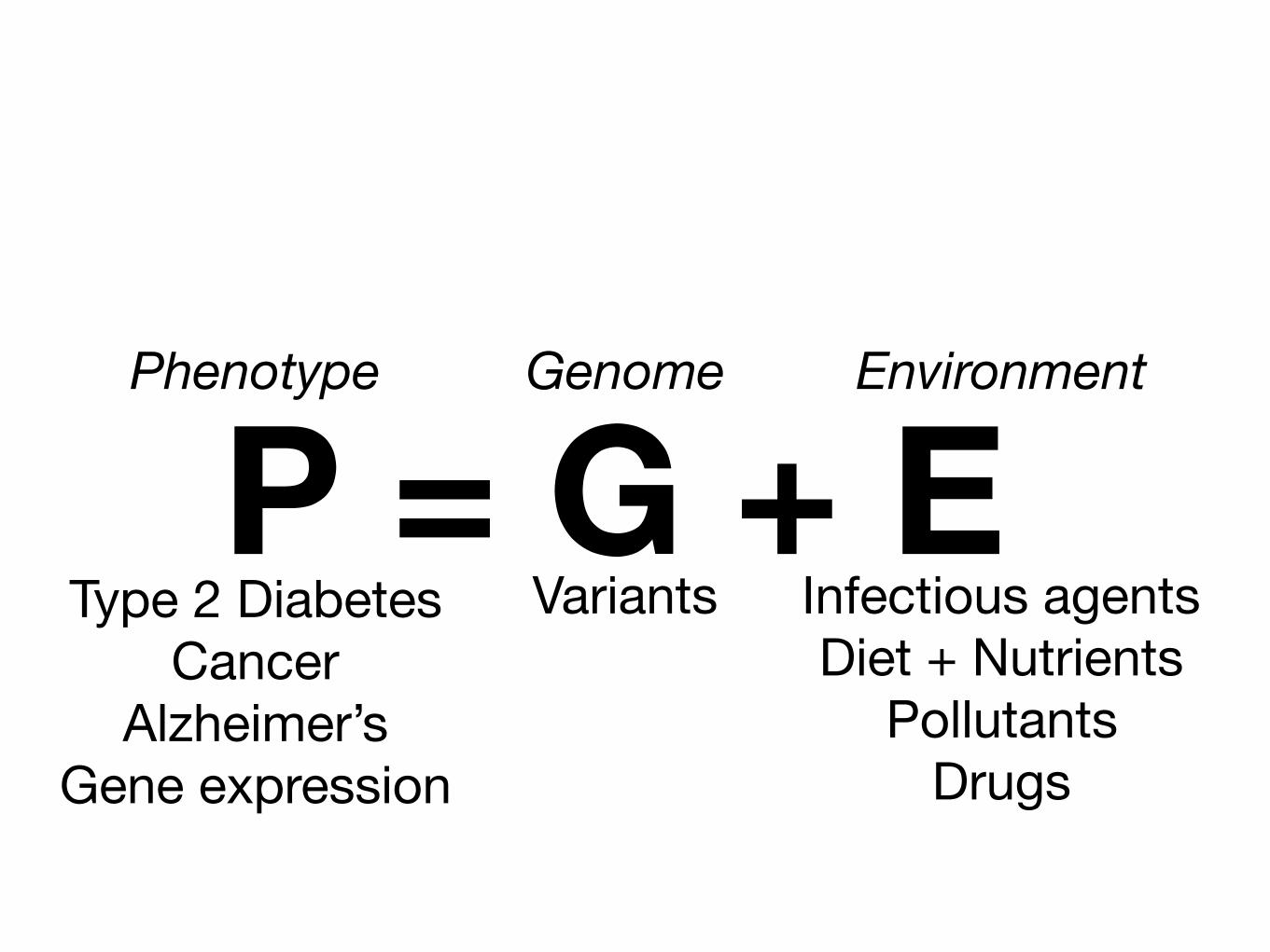
P = G + EType 2 Diabetes
CancerAlzheimer’s
Gene expression
Phenotype Genome
Variants
Environment
Infectious agentsDiet + Nutrients
PollutantsDrugs

We are great at G investigation!
2,940 (as of 6/1/17) 36,066 G-P associations
Genome-wide Association Studies (GWAS)https://www.ebi.ac.uk/gwas/
G

Nothing comparable to elucidate E influence!
E: ???
We lack high-throughput methods and data to discover new E in P…

A similar paradigm for discovery should existfor E!
Why?
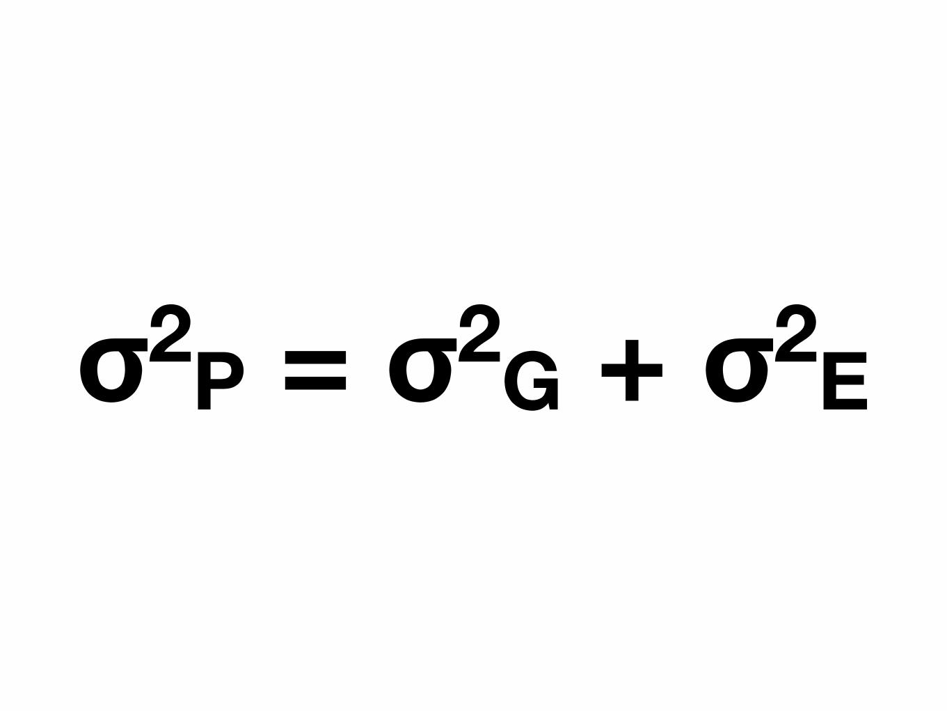
σ2P = σ2G + σ2E
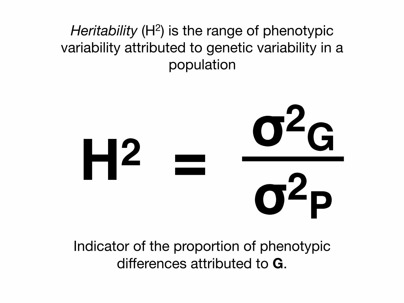
σ2Gσ2P H2 =
Heritability (H2) is the range of phenotypic variability attributed to genetic variability in a
population
Indicator of the proportion of phenotypic differences attributed to G.

Eye colorHair curliness
Type-1 diabetesHeight
SchizophreniaEpilepsy
Graves' diseaseCeliac disease
Polycystic ovary syndromeAttention deficit hyperactivity disorder
Bipolar disorderObesity
Alzheimer's diseaseAnorexia nervosa
PsoriasisBone mineral density
Menarche, age atNicotine dependence
Sexual orientationAlcoholism
LupusRheumatoid arthritis
Crohn's diseaseMigraine
Thyroid cancerAutism
Blood pressure, diastolicBody mass index
DepressionCoronary artery disease
InsomniaMenopause, age at
Heart diseaseProstate cancer
QT intervalBreast cancer
Ovarian cancerHangoverStrokeAsthma
Blood pressure, systolicHypertensionOsteoarthritis
Parkinson's diseaseLongevity
Type-2 diabetesGallstone diseaseTesticular cancer
Cervical cancerSciatica
Bladder cancerColon cancerLung cancerLeukemia
Stomach cancer
0 25 50 75 100Heritability: Var(G)/Var(Phenotype) Source: SNPedia.com
G estimates for burdensome diseases are low and variable: massive opportunity for high-throughput E discovery
Type 2 Diabetes
Heart Disease
Autism (50%???)

Eye colorHair curliness
Type-1 diabetesHeight
SchizophreniaEpilepsy
Graves' diseaseCeliac disease
Polycystic ovary syndromeAttention deficit hyperactivity disorder
Bipolar disorderObesity
Alzheimer's diseaseAnorexia nervosa
PsoriasisBone mineral density
Menarche, age atNicotine dependence
Sexual orientationAlcoholism
LupusRheumatoid arthritis
Crohn's diseaseMigraine
Thyroid cancerAutism
Blood pressure, diastolicBody mass index
DepressionCoronary artery disease
InsomniaMenopause, age at
Heart diseaseProstate cancer
QT intervalBreast cancer
Ovarian cancerHangoverStrokeAsthma
Blood pressure, systolicHypertensionOsteoarthritis
Parkinson's diseaseLongevity
Type-2 diabetesGallstone diseaseTesticular cancer
Cervical cancerSciatica
Bladder cancerColon cancerLung cancerLeukemia
Stomach cancer
0 25 50 75 100Heritability: Var(G)/Var(Phenotype) Source: SNPedia.com
G estimates for complex traits are low and variable: massive opportunity for high-throughput E discovery
σ2E : Exposome!
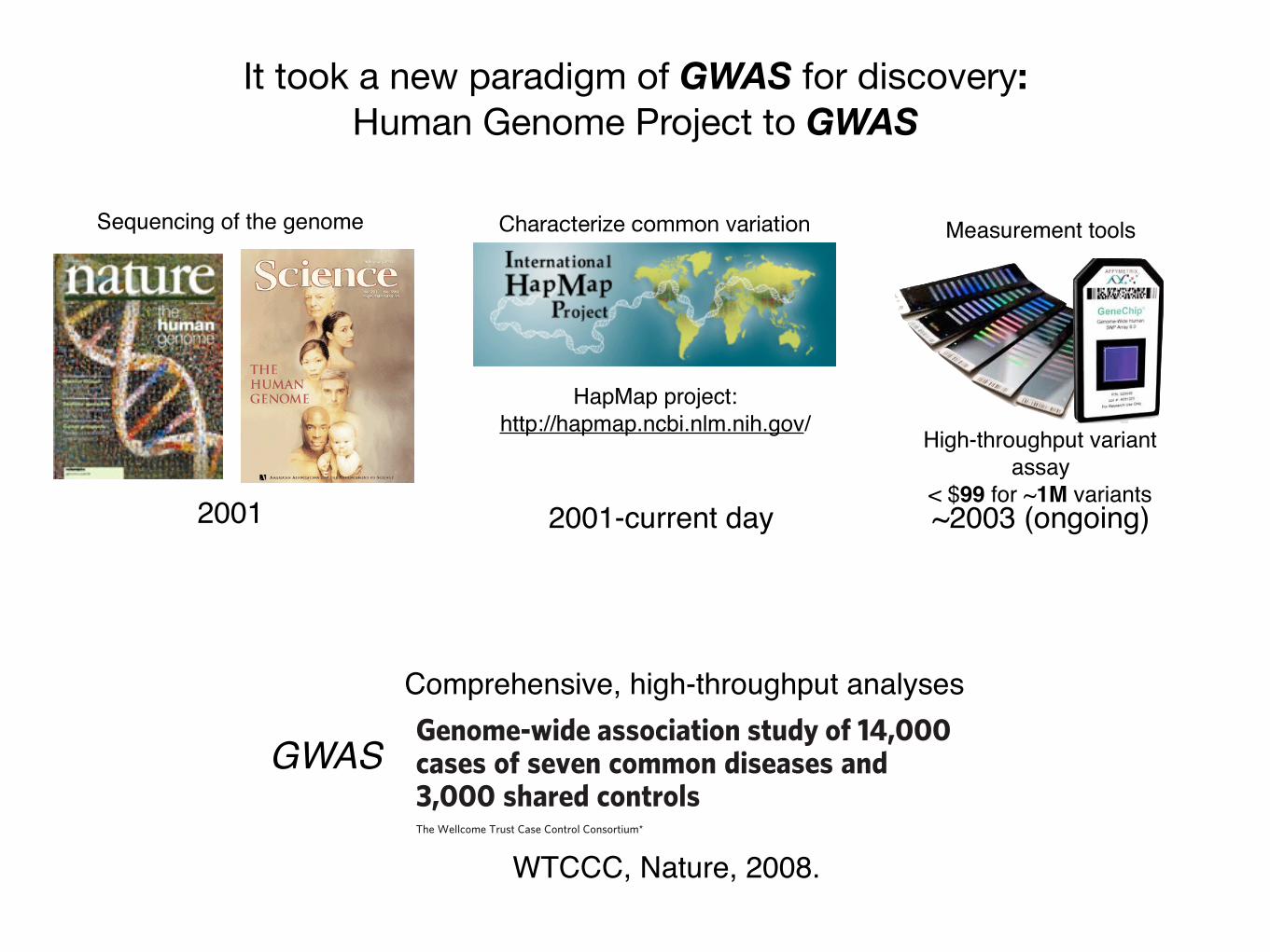
It took a new paradigm of GWAS for discovery: Human Genome Project to GWAS
Sequencing of the genome
2001
HapMap project:http://hapmap.ncbi.nlm.nih.gov/
Characterize common variation
2001-current day
High-throughput variant assay
< $99 for ~1M variants
Measurement tools
~2003 (ongoing)
ARTICLES
Genome-wide association study of 14,000cases of seven common diseases and3,000 shared controlsThe Wellcome Trust Case Control Consortium*
There is increasing evidence that genome-wide association (GWA) studies represent a powerful approach to theidentification of genes involved in common human diseases.We describe a joint GWAstudy (using the Affymetrix GeneChip500KMapping Array Set) undertaken in the British population, which has examined,2,000 individuals for each of 7 majordiseases and a shared set of ,3,000 controls. Case-control comparisons identified 24 independent association signals atP, 53 1027: 1 in bipolar disorder, 1 in coronary artery disease, 9 in Crohn’s disease, 3 in rheumatoid arthritis, 7 in type 1diabetes and 3 in type 2 diabetes. On the basis of prior findings and replication studies thus-far completed, almost all of thesesignals reflect genuine susceptibility effects. We observed association at many previously identified loci, and foundcompelling evidence that some loci confer risk for more than one of the diseases studied. Across all diseases, we identified alarge number of further signals (including 58 loci with single-point P values between 1025 and 53 1027) likely to yieldadditional susceptibility loci. The importance of appropriately large samples was confirmed by the modest effect sizesobserved at most loci identified. This study thus represents a thorough validation of the GWA approach. It has alsodemonstrated that careful use of a shared control group represents a safe and effective approach to GWA analyses ofmultiple disease phenotypes; has generated a genome-wide genotype database for future studies of common diseases in theBritish population; and shown that, provided individuals with non-European ancestry are excluded, the extent of populationstratification in the British population is generally modest. Our findings offer new avenues for exploring the pathophysiologyof these important disorders. We anticipate that our data, results and software, which will be widely available to otherinvestigators, will provide a powerful resource for human genetics research.
Despite extensive research efforts for more than a decade, the geneticbasis of common humandiseases remains largely unknown. Althoughthere have been some notable successes1, linkage and candidate geneassociation studies have often failed to deliver definitive results. Yetthe identification of the variants, genes and pathways involved inparticular diseases offers a potential route to new therapies, improveddiagnosis and better disease prevention. For some time it has beenhoped that the advent of genome-wide association (GWA) studieswould provide a successful new tool for unlocking the genetic basisof many of these common causes of humanmorbidity andmortality1.
Three recent advances mean that GWA studies that are powered todetect plausible effect sizes are now possible2. First, the InternationalHapMap resource3, which documents patterns of genome-wide vari-ation and linkage disequilibrium in four population samples, greatlyfacilitates both the design and analysis of association studies. Second,the availability of dense genotyping chips, containing sets of hundreds ofthousands of single nucleotide polymorphisms (SNPs) that providegood coverage of much of the human genome, means that for the firsttimeGWAstudies for thousandsof cases andcontrols are technically andfinancially feasible. Third, appropriately large and well-characterizedclinical samples have been assembled for many common diseases.
The Wellcome Trust Case Control Consortium (WTCCC) wasformed with a view to exploring the utility, design and analyses ofGWA studies. It brought together over 50 research groups from theUK that are active in researching the genetics of common humandiseases, with expertise ranging from clinical, through genotyping, to
informatics and statistical analysis. Here we describe the main experi-ment of the consortium: GWA studies of 2,000 cases and 3,000 sharedcontrols for 7 complex human diseases of major public health import-ance—bipolar disorder (BD), coronary artery disease (CAD), Crohn’sdisease (CD), hypertension (HT), rheumatoid arthritis (RA), type 1diabetes (T1D), and type 2 diabetes (T2D). Two further experimentsundertaken by the consortium will be reported elsewhere: a GWAstudy for tuberculosis in 1,500 cases and 1,500 controls, sampled fromThe Gambia; and an association study of 1,500 common controls with1,000 cases for each of breast cancer, multiple sclerosis, ankylosingspondylitis and autoimmune thyroid disease, all typed at around15,000 mainly non-synonymous SNPs. By simultaneously studyingseven diseases with differing aetiologies, we hoped to develop insights,not only into the specific genetic contributions to each of the diseases,but also into differences in allelic architecture across the diseases. Afurther major aim was to address important methodological issues ofrelevance to all GWA studies, such as quality control, design and ana-lysis. In addition to our main association results, we address several ofthese issues below, including the choice of controls for genetic studies,the extent of population structure within Great Britain, sample sizesnecessary to detect genetic effects of varying sizes, and improvements ingenotype-calling algorithms and analytical methods.
Samples and experimental analyses
Individuals included in the study were living within England,Scotland and Wales (‘Great Britain’) and the vast majority had
*Lists of participants and affiliations appear at the end of the paper.
Vol 447 |7 June 2007 |doi:10.1038/nature05911
661Nature ©2007 Publishing Group
WTCCC, Nature, 2008.
Comprehensive, high-throughput analyses
GWAS

What is a Genome-Wide Association Study (GWAS)?: Data-driven search for G factors in P
Methods), and excluded 153 individuals on this basis. We nextlooked for evidence of population heterogeneity by studying allelefrequency differences between the 12 broad geographical regions(defined in Supplementary Fig. 4). The results for these 11-d.f. testsand associated quantile-quantile plots are shown in Fig. 2. Wide-spread small differences in allele frequencies are evident as anincreased slope of the line (Fig. 2b); in addition, a few loci showmuchlarger differences (Fig. 2a and Supplementary Fig. 6).
Thirteen genomic regions showing strong geographical variationare listed in Table 1, and Supplementary Fig. 7 shows theway in whichtheir allele frequencies vary geographically. The predominant patternis variation along a NW/SE axis. The most likely cause for thesemarked geographical differences is natural selection, most plausiblyin populations ancestral to those now in the UK. Variation due toselection has previously been implicated at LCT (lactase) and majorhistocompatibility complex (MHC)7–9, andwithin-UKdifferentiationat 4p14 has been found independently10, but others seem to be newfindings. All but three of the regions contain known genes. Aside from
evolutionary interest, genes showing evidence of natural selection areparticularly interesting for the biology of traits such as infectious dis-eases; possible targets for selection include NADSYN1 (NAD synthe-tase 1) at 11q13, which could have a role in prevention of pellagra, aswell as TLR1 (toll-like receptor 1) at 4p14, for which a role in thebiology of tuberculosis and leprosy has been suggested10.
There may be important population structure that is not wellcaptured by current geographical region of residence. Presentimplementations of strongly model-based approaches such asSTRUCTURE11,12 are impracticable for data sets of this size, and wereverted to the classical method of principal components13,14, using asubset of 197,175 SNPs chosen to reduce inter-locus linkage disequi-librium. Nevertheless, four of the first six principal componentsclearly picked up effects attributable to local linkage disequilibriumrather than genome-wide structure. The remaining two componentsshow the same predominant geographical trend from NW to SE but,perhaps unsurprisingly, London is set somewhat apart (Supplemen-tary Fig. 8).
The overall effect of population structure on our associationresults seems to be small, once recent migrants from outsideEurope are excluded. Estimates of over-dispersion of the associationtrend test statistics (usually denoted l; ref. 15) ranged from 1.03 and1.05 for RA and T1D, respectively, to 1.08–1.11 for the remainingdiseases. Some of this over-dispersion could be due to factors otherthan structure, and this possibility is supported by the fact that inclu-sion of the two ancestry informative principal components as cov-ariates in the association tests reduced the over-dispersion estimatesonly slightly (Supplementary Table 6), as did stratification by geo-graphical region. This impression is confirmed on noting thatP values with and without correction for structure are similar(Supplementary Fig. 9). We conclude that, for most of the genome,population structure has at most a small confounding effect in ourstudy, and as a consequence the analyses reported below do notcorrect for structure. In principle, apparent associations in the fewgenomic regions identified in Table 1 as showing strong geographicaldifferentiation should be interpreted with caution, but none arose inour analyses.
Disease association results
We assessed evidence for association in several ways (see Methods fordetails), drawing on both classical and bayesian statistical approaches.For polymorphic SNPs on the Affymetrix chip, we performed trendtests (1 degree of freedom16) and general genotype tests (2 degrees offreedom16, referred to as genotypic) between each case collection andthe pooled controls, and calculated analogous Bayes factors. Thereare examples from animal models where genetic effects act differentlyin males and females17, and to assess this in our data we applied a
−log
10(P
)
0
5
10
15
Chromosome
22 X212019181716151413121110987654321
3020
20
100
0
40
80
60
40
100
Obs
erve
d te
st s
tatis
tic
Expected chi-squared value
a
b
Figure 2 | Genome-wide picture of geographic variation. a, P values for the11-d.f. test for difference in SNP allele frequencies between geographicalregions, within the 9 collections. SNPs have been excluded using the projectquality control filters described inMethods. Green dots indicate SNPs with aP value,13 1025. b, Quantile-quantile plots of these test statistics. SNPs atwhich the test statistic exceeds 100 are represented by triangles at the top ofthe plot, and the shaded region is the 95% concentration band (seeMethods). Also shown in blue is the quantile-quantile plot resulting fromremoval of all SNPs in the 13 most differentiated regions (Table 1).
Table 1 | Highly differentiated SNPs
Chromosome Genes Region (Mb) SNP Position P value
2q21 LCT 135.16–136.82 rs1042712 136,379,576 5.54 3 10213
4p14 TLR1, TLR6, TLR10 38.51–38.74 rs7696175 386,43,552 1.51 3 10212
4q28 137.97–138.01 rs1460133 137,999,953 4.43 3 10208
6p25 IRF4 0.32–0.42 rs9378805 362,727 5.39 3 10213
6p21 HLA 31.10–31.55 rs3873375 31,359,339 1.07 3 10211
9p24 DMRT1 0.86–0.88 rs11790408 866,418 4.96 3 10207
11p15 NAV2 19.55–19.70 rs12295525 19,661,808 7.44 3 10208
11q13 NADSYN1, DHCR7 70.78–70.93 rs12797951 70,820,914 3.01 3 10208
12p13 DYRK4,AKAP3,NDUFA9,RAD51AP1,GALNT8
4.37–4.82 rs10774241 45,537,27 2.73 3 10208
14q12 HECTD1,AP4S1,STRN3 30.41–31.03 rs17449560 30,598,823 1.46 3 10207
19q13 GIPR,SNRPD2,QPCTL,SIX5,DMPK,DMWD,RSHL1,SYMPK,FOXA3
50.84–51.09 rs3760843 50,980,546 4.19 3 10207
20q12 38.30–38.77 rs2143877 38,526,309 1.12 3 10209
Xp22 2.06–2.08 rs6644913 2,061,160 1.23 3 10207
Properties of SNPs that show large allele frequency differences between samples of individuals from 12 regions across Great Britain. Regions showing differentiated SNPs are givenwith details of theSNPwith the smallest P value in each region for differentiation on the 11-d.f. test of differences in SNP allele frequencies between geographical regions, within the 9 collections. Cluster plots for theseSNPs have been examined visually. Signal plots appear in Supplementary Information. Positions are in NCBI build-35 coordinates.
NATURE |Vol 447 |7 June 2007 ARTICLES
663Nature ©2007 Publishing Group
WTCCC Nature, 2007
AA Aa aacase
control
Robust, transparent, and comprehensive search for G in P
Methods), and excluded 153 individuals on this basis. We nextlooked for evidence of population heterogeneity by studying allelefrequency differences between the 12 broad geographical regions(defined in Supplementary Fig. 4). The results for these 11-d.f. testsand associated quantile-quantile plots are shown in Fig. 2. Wide-spread small differences in allele frequencies are evident as anincreased slope of the line (Fig. 2b); in addition, a few loci showmuchlarger differences (Fig. 2a and Supplementary Fig. 6).
Thirteen genomic regions showing strong geographical variationare listed in Table 1, and Supplementary Fig. 7 shows theway in whichtheir allele frequencies vary geographically. The predominant patternis variation along a NW/SE axis. The most likely cause for thesemarked geographical differences is natural selection, most plausiblyin populations ancestral to those now in the UK. Variation due toselection has previously been implicated at LCT (lactase) and majorhistocompatibility complex (MHC)7–9, andwithin-UKdifferentiationat 4p14 has been found independently10, but others seem to be newfindings. All but three of the regions contain known genes. Aside from
evolutionary interest, genes showing evidence of natural selection areparticularly interesting for the biology of traits such as infectious dis-eases; possible targets for selection include NADSYN1 (NAD synthe-tase 1) at 11q13, which could have a role in prevention of pellagra, aswell as TLR1 (toll-like receptor 1) at 4p14, for which a role in thebiology of tuberculosis and leprosy has been suggested10.
There may be important population structure that is not wellcaptured by current geographical region of residence. Presentimplementations of strongly model-based approaches such asSTRUCTURE11,12 are impracticable for data sets of this size, and wereverted to the classical method of principal components13,14, using asubset of 197,175 SNPs chosen to reduce inter-locus linkage disequi-librium. Nevertheless, four of the first six principal componentsclearly picked up effects attributable to local linkage disequilibriumrather than genome-wide structure. The remaining two componentsshow the same predominant geographical trend from NW to SE but,perhaps unsurprisingly, London is set somewhat apart (Supplemen-tary Fig. 8).
The overall effect of population structure on our associationresults seems to be small, once recent migrants from outsideEurope are excluded. Estimates of over-dispersion of the associationtrend test statistics (usually denoted l; ref. 15) ranged from 1.03 and1.05 for RA and T1D, respectively, to 1.08–1.11 for the remainingdiseases. Some of this over-dispersion could be due to factors otherthan structure, and this possibility is supported by the fact that inclu-sion of the two ancestry informative principal components as cov-ariates in the association tests reduced the over-dispersion estimatesonly slightly (Supplementary Table 6), as did stratification by geo-graphical region. This impression is confirmed on noting thatP values with and without correction for structure are similar(Supplementary Fig. 9). We conclude that, for most of the genome,population structure has at most a small confounding effect in ourstudy, and as a consequence the analyses reported below do notcorrect for structure. In principle, apparent associations in the fewgenomic regions identified in Table 1 as showing strong geographicaldifferentiation should be interpreted with caution, but none arose inour analyses.
Disease association results
We assessed evidence for association in several ways (see Methods fordetails), drawing on both classical and bayesian statistical approaches.For polymorphic SNPs on the Affymetrix chip, we performed trendtests (1 degree of freedom16) and general genotype tests (2 degrees offreedom16, referred to as genotypic) between each case collection andthe pooled controls, and calculated analogous Bayes factors. Thereare examples from animal models where genetic effects act differentlyin males and females17, and to assess this in our data we applied a
−log
10(P
)
0
5
10
15
Chromosome
22 X212019181716151413121110987654321
3020
20
100
0
40
80
60
40
100
Obs
erve
d te
st s
tatis
tic
Expected chi-squared value
a
b
Figure 2 | Genome-wide picture of geographic variation. a, P values for the11-d.f. test for difference in SNP allele frequencies between geographicalregions, within the 9 collections. SNPs have been excluded using the projectquality control filters described inMethods. Green dots indicate SNPs with aP value,13 1025. b, Quantile-quantile plots of these test statistics. SNPs atwhich the test statistic exceeds 100 are represented by triangles at the top ofthe plot, and the shaded region is the 95% concentration band (seeMethods). Also shown in blue is the quantile-quantile plot resulting fromremoval of all SNPs in the 13 most differentiated regions (Table 1).
Table 1 | Highly differentiated SNPs
Chromosome Genes Region (Mb) SNP Position P value
2q21 LCT 135.16–136.82 rs1042712 136,379,576 5.54 3 10213
4p14 TLR1, TLR6, TLR10 38.51–38.74 rs7696175 386,43,552 1.51 3 10212
4q28 137.97–138.01 rs1460133 137,999,953 4.43 3 10208
6p25 IRF4 0.32–0.42 rs9378805 362,727 5.39 3 10213
6p21 HLA 31.10–31.55 rs3873375 31,359,339 1.07 3 10211
9p24 DMRT1 0.86–0.88 rs11790408 866,418 4.96 3 10207
11p15 NAV2 19.55–19.70 rs12295525 19,661,808 7.44 3 10208
11q13 NADSYN1, DHCR7 70.78–70.93 rs12797951 70,820,914 3.01 3 10208
12p13 DYRK4,AKAP3,NDUFA9,RAD51AP1,GALNT8
4.37–4.82 rs10774241 45,537,27 2.73 3 10208
14q12 HECTD1,AP4S1,STRN3 30.41–31.03 rs17449560 30,598,823 1.46 3 10207
19q13 GIPR,SNRPD2,QPCTL,SIX5,DMPK,DMWD,RSHL1,SYMPK,FOXA3
50.84–51.09 rs3760843 50,980,546 4.19 3 10207
20q12 38.30–38.77 rs2143877 38,526,309 1.12 3 10209
Xp22 2.06–2.08 rs6644913 2,061,160 1.23 3 10207
Properties of SNPs that show large allele frequency differences between samples of individuals from 12 regions across Great Britain. Regions showing differentiated SNPs are givenwith details of theSNPwith the smallest P value in each region for differentiation on the 11-d.f. test of differences in SNP allele frequencies between geographical regions, within the 9 collections. Cluster plots for theseSNPs have been examined visually. Signal plots appear in Supplementary Information. Positions are in NCBI build-35 coordinates.
NATURE |Vol 447 |7 June 2007 ARTICLES
663Nature ©2007 Publishing Group
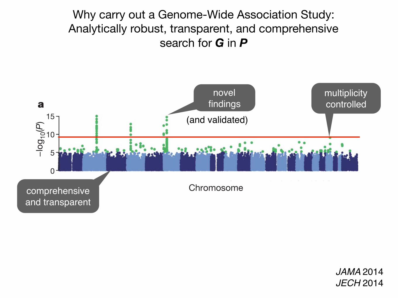
comprehensive and transparent
multiplicity controlled
novel findings
(and validated)
JAMA 2014JECH 2014
Why carry out a Genome-Wide Association Study: Analytically robust, transparent, and comprehensive
search for G in P
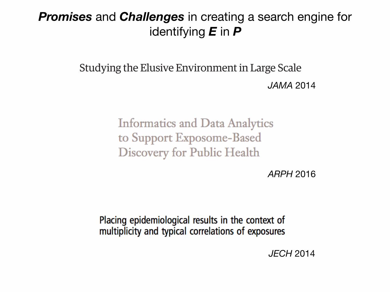
Promises and Challenges in creating a search engine for identifying E in P
Copyright 2014 American Medical Association. All rights reserved.
Studying the Elusive Environment in Large Scale
It is possible that more than 50% of complex disease riskis attributed to differences in an individual’s environment.1
Air pollution, smoking, and diet are documented environ-mental factors affecting health, yet these factors are buta fraction of the “exposome,” the totality of the exposureload occurring throughout a person’s lifetime.1 Investigat-ing one or a handful of exposures at a time has led to ahighly fragmented literature of epidemiologic associa-tions. Much of that literature is not reproducible, and se-lective reporting may be a major reason for the lack of re-producibility. A new model is required to discoverenvironmental exposures associated with disease whilemitigating possibilities of selective reporting.
To remedy the lack of reproducibility and concerns ofvalidity, multiple personal exposures can be assessed si-multaneously in terms of their association with a condi-tion or disease of interest; the strongest associations canthen be tentatively validated in independent data sets(eg, as done in references 2 and 3).2,3 The main advan-tages of this process include the ability to search the listof exposures and adjust for multiplicity systematically andreport all the probed associations instead of only the mostsignificant results. The term “environment-wide associa-tion studies” (EWAS) has been used to describe this ap-proach (an analogy to genome-wide association stud-ies). For example, Wang et al4 screened more than 2000chemicals in serum to discover endogenous exposures as-sociated with risk for cardiovascular disease.
There are notable hurdles in analyzing “big” environ-mental data. These same problems affect epidemiologyof 1-risk-factor-at-a-time, but in EWAS their prevalence be-comes more clearly manifest at large scale. When study-ing hundreds and thousands of exposures, tens and hun-dreds of associations often emerge that pass conventionalstatistical thresholds. Yet most of these seemingly statis-ticallyrobustassociationsarecorrelatesonly,notcausalas-sociations. Reverse causality and confounding may under-lie most of the observed strong correlations.
Based on the enormous number of potential interre-lated correlations between multiple environmental expo-sures (depicted by edges in the Figure), it is uncertainwhether there was ever any reasonable hope for tradi-tionalepidemiologytouserationalthinking,biologicalplau-sibility, or some other reasoning to select and documentrisk exposures one at a time. For example, smoking (mea-sured by cotinine levels) is clearly harmful, but it is also cor-related with dozens of other exposures (Figure, A). Seem-ingly harmful associations of these exposures with diversehealth outcomes may simply be attributable to their cor-relation with smoking. Pollutants such as mercury(Figure, B) or cadmium (Figure, C) may have multiple cor-relations with diverse seemingly “healthy” nutrients andother exposures. Moreover, any intervention that tries toinfluence one exposure node may inadvertently influ-ence many others that are correlated. For example, from
the EWAS vantage point, intervening on β-carotene(Figure, D) seems a futile exercise given its complex rela-tionship with other nutrients and pollutants.
Giventhiscomplexity,howcanstudiesofenvironmen-tal risk move forward? First, EWAS analyses should be ap-plied to multiple data sets, and consistency can be formallyexaminedforallassessedcorrelations.Second,thetempo-ral relationship between exposure and changes in healthparameters may offer helpful hints about which of the sig-nals are more than simple correlations. Third, standardizedadjustedanalyses, inwhichadjustmentsareperformedsys-tematically and in the same way across multiple data sets,may also help. This is in stark contrast with the currentmodel,wherebymostepidemiologicstudiesusesingledatasetswithoutreplicationaswellasnon–time-dependentas-sessments, and reported adjustments are markedly differ-ent across reports and data sets, even those performed bythe same team (different approaches increase validity butmust be reconciled and assimilated).
However, eventually for most environmental cor-relates, there may be unsurpassable difficulty establish-ing potential causal inferences based on observationaldata alone. Factors that seem protective may some-times be tested in randomized trials. The complexity ofthe multiple correlations also highlights the challengethat intervening to modify 1 putative risk factor also mayinadvertently affect multiple other correlated factors.Even when a seemingly simple intervention is tested inrandomized trials (affecting a single risk factor among themany correlations), the intervention is not really simple.In essence what is tested are multiple perturbations offactors correlated with the one targeted for interven-tion. This means that randomized trials of interven-tions on putative protective environmental exposures(eg, diet or lifestyle) should be repeated in diverse popu-lations for which the interrelated correlations might bedifferent, before considered widely generalizable.
The EWAS model can be extended and improved.To capture time dependence, investigations must ac-commodate measurement of multiple environmental ex-posures at different times in the lifespan, particularly indevelopment, and new analytical methods must be ableto capture the complex temporal relationship betweenmultiple exposures and future disease risk.5 Second, littleis known about how environment interacts with the ge-nome. The current literature on gene-environment in-teraction is highly fragmented, nonsystematic, and sub-ject to selective reporting, suggesting the need forinterdisciplinary gene-environment–wide associationstudies.6 In addition, quality of measurements will dic-tate the breadth of any environmental research effort.However, quantitative and inexpensive methods to mea-sure many environmental factors in a high-throughputmanner (unlike genetic chips) are lacking. Mirroring theevolution of genomic measurements, this may change.
VIEWPOINT
Chirag J. Patel, PhDCenter for BiomedicalInformatics, HarvardMedical School,Boston, Massachusetts.
John P. A. Ioannidis,MD, DScStanford PreventionResearch Center,Department of HealthResearch and Policy,Department ofMedicine, StanfordUniversity School ofMedicine, Stanford,California, Departmentof Statistics, StanfordUniversity School ofHumanities andSciences, Stanford,California, andMeta-ResearchInnovation Center atStanford (METRICS),Stanford, California.
CorrespondingAuthor: John P. A.Ioannidis, MD, DSc,Stanford University,1265 Welch Rd, MSOBX306, Stanford, CA94305 ([email protected]).
Opinion
jama.com JAMA June 4, 2014 Volume 311, Number 21 2173
Copyright 2014 American Medical Association. All rights reserved.
Downloaded From: http://jama.jamanetwork.com/ by a Harvard University User on 06/03/2014
JAMA 2014
ARPH 2016
JECH 2014
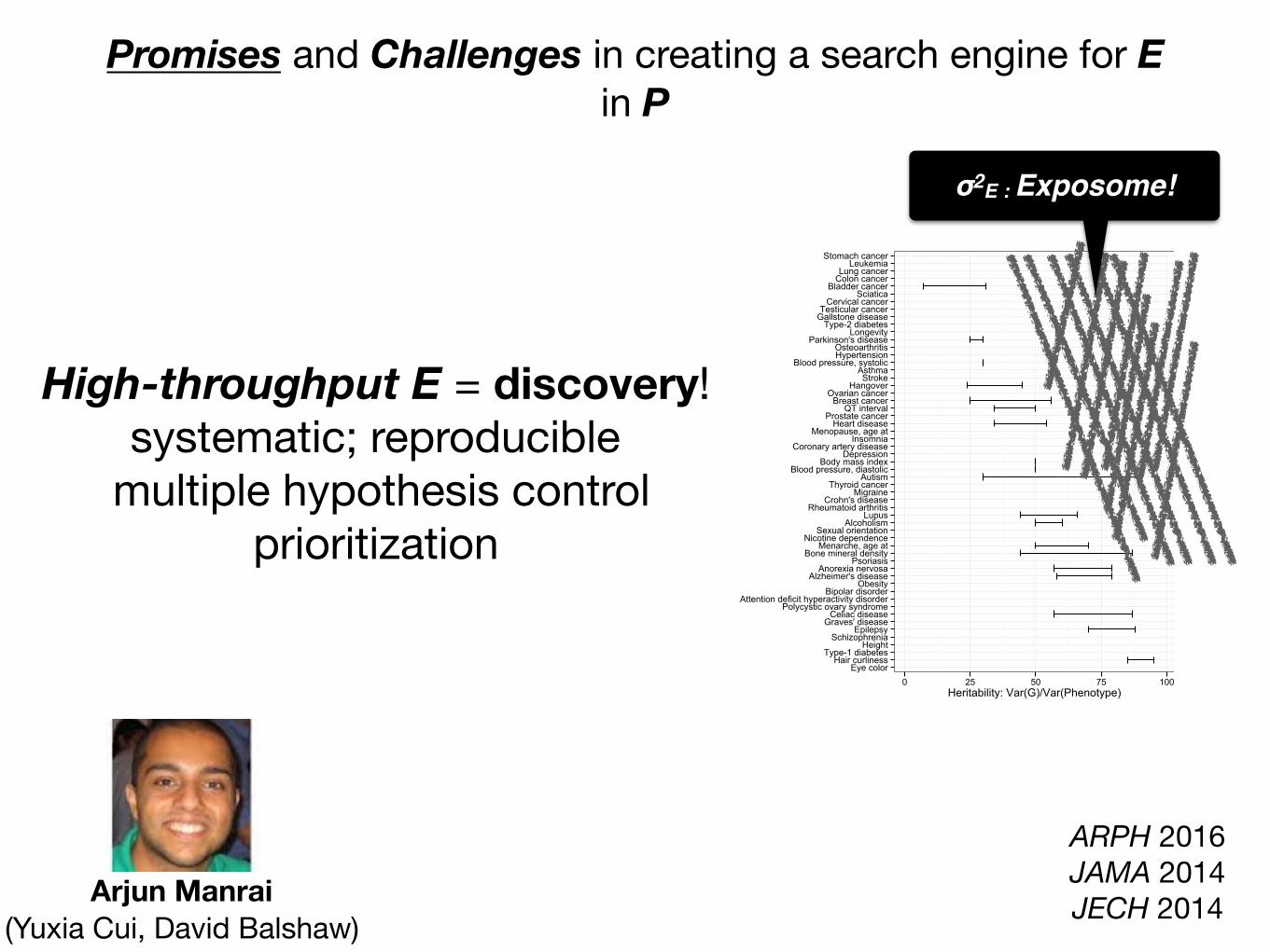
Promises and Challenges in creating a search engine for E in P
High-throughput E = discovery!systematic; reproducible
multiple hypothesis controlprioritization
Eye colorHair curliness
Type-1 diabetesHeight
SchizophreniaEpilepsy
Graves' diseaseCeliac disease
Polycystic ovary syndromeAttention deficit hyperactivity disorder
Bipolar disorderObesity
Alzheimer's diseaseAnorexia nervosa
PsoriasisBone mineral density
Menarche, age atNicotine dependence
Sexual orientationAlcoholism
LupusRheumatoid arthritis
Crohn's diseaseMigraine
Thyroid cancerAutism
Blood pressure, diastolicBody mass index
DepressionCoronary artery disease
InsomniaMenopause, age at
Heart diseaseProstate cancer
QT intervalBreast cancer
Ovarian cancerHangoverStrokeAsthma
Blood pressure, systolicHypertensionOsteoarthritis
Parkinson's diseaseLongevity
Type-2 diabetesGallstone diseaseTesticular cancer
Cervical cancerSciatica
Bladder cancerColon cancerLung cancerLeukemia
Stomach cancer
0 25 50 75 100Heritability: Var(G)/Var(Phenotype)
Arjun Manrai (Yuxia Cui, David Balshaw)
ARPH 2016JAMA 2014JECH 2014
σ2E : Exposome!

Examples of exposome-driven discovery machinery, or EWASs
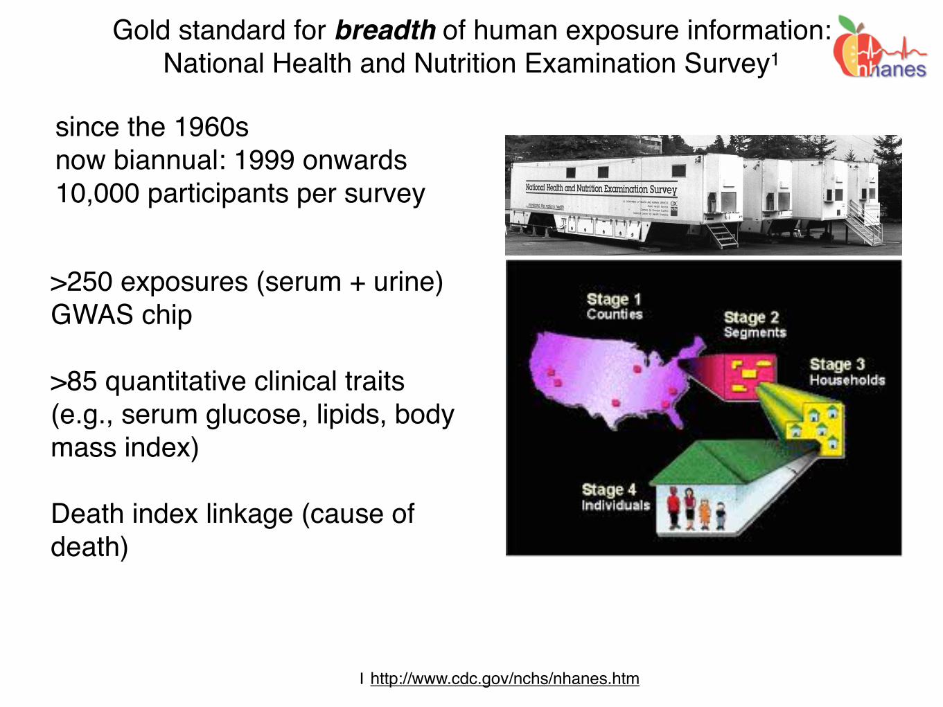
Gold standard for breadth of human exposure information: National Health and Nutrition Examination Survey1
since the 1960snow biannual: 1999 onwards10,000 participants per survey
Introduction
The National Health and Nutrition Examination Survey (NHANES) is a program of studiesdesigned to assess the health and nutritional status of adults and children in the United States. The survey is unique in that it com-bines interviews and physical examinations. NHANES is a major program of the National Center for Health Statistics (NCHS). NCHS is part of the Centers for Disease Control and Prevention (CDC) and has the responsibility for producing vital and health statistics for the Nation.
The NHANES program began in the early 1960s and has been conducted as a series of sur-veys focusing on different population groups or health topics. In 1999, the survey became a con-tinuous program that has a changing focus on a variety of health and nutrition measurements to meet emerging needs. The survey examines a nationally representative sample of about 5,000 persons each year. These persons are located in counties across the country, 15 of which are visited each year.
The NHANES interview includes demographic, socioeconomic, dietary, and health-related questions. The examination component consists of medical, dental, and physiological measure-ments, as well as laboratory tests administered by highly trained medical personnel.
Findings from this survey will be used to de-termine the prevalence of major diseases and risk factors for diseases. Information will be used to assess nutritional status and its associ-ation with health promotion and disease pre-vention. NHANES findings are also the basis for national standards for such measurements as height, weight, and blood pressure. Data from this survey will be used in epidemiologi-cal studies and health sciences research, which help develop sound public health policy,
direct and design health programs and services, and expand the health knowl-edge for the Nation.
Survey Content
As in past health examination surveys, data will be collected on the prevalence of chron-ic conditions in the population. Estimates for previously undiagnosed conditions, as well as those known to and reported by respon-dents, are produced through the survey. Such information is a particular strength of the NHANES program.
Risk factors, those aspects of a person’s life-style, constitution, heredity, or environment that may increase the chances of developing a certain disease or condition, will be examined. Smoking, alcohol consumption, sexual practices, drug use, physical fitness and activity, weight, and dietary intake will be studied. Data on certain aspects of reproductive health, such as use of oral contraceptives and breastfeeding practices, will also be collected.
The diseases, medical conditions, and health indicators to be studied include:
• Anemia• Cardiovascular disease• Diabetes• Environmental exposures• Eye diseases• Hearing loss• Infectious diseases• Kidney disease• Nutrition• Obesity• Oral health• Osteoporosis
The sample for the survey is selected to represent the U.S. population of all ages. To produce reli-able statistics, NHANES over-samples persons 60 and older, African Americans, and Hispanics.
Since the United States has experienced dramatic growth in the number of older people during this century, the aging population has major impli-cations for health care needs, public policy, and research priorities. NCHS is working with public health agencies to increase the knowledge of the health status of older Americans. NHANES has a primary role in this endeavor.
All participants visit the physician. Dietary inter-views and body measurements are included for everyone. All but the very young have a blood sample taken and will have a dental screening. Depending upon the age of the participant, the rest of the examination includes tests and proce-dures to assess the various aspects of health listed above. In general, the older the individual, the more extensive the examination.
Survey Operations
Health interviews are conducted in respondents’ homes. Health measurements are performed in specially-designed and equipped mobile centers, which travel to locations throughout the country. The study team consists of a physician, medical and health technicians, as well as dietary and health interviewers. Many of the study staff are bilingual (English/Spanish).
An advanced computer system using high-end servers, desktop PCs, and wide-area networking collect and process all of the NHANES data, nearly eliminating the need for paper forms and manual coding operations. This system allows interviewers to use note-book computers with electronic pens. The staff at the mobile center can automatically transmit data into data bases through such devices as digital scales and stadiometers. Touch-sensi-tive computer screens let respondents enter their own responses to certain sensitive ques-tions in complete privacy. Survey information is available to NCHS staff within 24 hours of collection, which enhances the capability of collecting quality data and increases the speed with which results are released to the public.
In each location, local health and government officials are notified of the upcoming survey. Households in the study area receive a letter from the NCHS Director to introduce the survey. Local media may feature stories about the survey.
NHANES is designed to facilitate and en-courage participation. Transportation is provided to and from the mobile center if necessary. Participants receive compensation and a report of medical findings is given to each participant. All information collected in the survey is kept strictly confidential. Privacy is protected by public laws.
Uses of the Data
Information from NHANES is made available through an extensive series of publications and articles in scientific and technical journals. For data users and researchers throughout the world, survey data are available on the internet and on easy-to-use CD-ROMs.
Research organizations, universities, health care providers, and educators benefit from survey information. Primary data users are federal agencies that collaborated in the de-sign and development of the survey. The National Institutes of Health, the Food and Drug Administration, and CDC are among the agencies that rely upon NHANES to provide data essential for the implementation and evaluation of program activities. The U.S. Department of Agriculture and NCHS coop-erate in planning and reporting dietary and nutrition information from the survey.
NHANES’ partnership with the U.S. Environ-mental Protection Agency allows continued study of the many important environmental influences on our health.
• Physical fitness and physical functioning• Reproductive history and sexual behavior• Respiratory disease (asthma, chronic bron- chitis, emphysema)• Sexually transmitted diseases • Vision
1 http://www.cdc.gov/nchs/nhanes.htm
>250 exposures (serum + urine)GWAS chip
>85 quantitative clinical traits (e.g., serum glucose, lipids, body mass index)
Death index linkage (cause of death)

Gold standard for breadth of exposure & behavior data: National Health and Nutrition Examination Survey
Nutrients and Vitaminsvitamin D, carotenes
Infectious Agentshepatitis, HIV, Staph. aureus
Plastics and consumablesphthalates, bisphenol A
Physical Activitye.g., stepsPesticides and pollutants
atrazine; cadmium; hydrocarbons
Drugsstatins; aspirin
What E are associated with aging: all-cause mortality and
telomere length?
Int J Epidem 2013Int J Epidem 2016

How does it work?: Searching for exposures and behaviors associated with all-
cause mortality.
NHANES: 1999-2004National Death Index linked mortality
249 behaviors and exposures (serum/urine/self-report)
NHANES: 1999-2001N=330 to 6008 (26 to 655 deaths)
~5.5 years of followup
Cox proportional hazardsbaseline exposure and time to death
False discovery rate < 5%
NHANES: 2003-2004N=177 to 3258 (20-202 deaths)
~2.8 years of followup
p < 0.05
Int J Epidem 2013
?
Variance explained (R2):Proportion of variance in death correlated with E
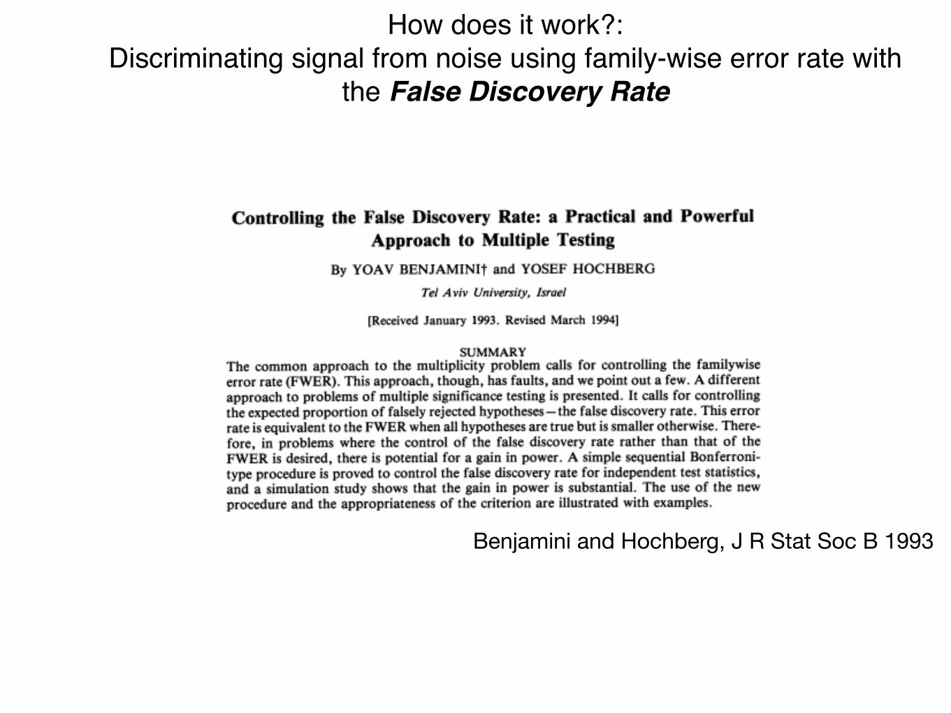
How does it work?: Discriminating signal from noise using family-wise error rate with
the False Discovery Rate
Benjamini and Hochberg, J R Stat Soc B 1993

Noble, Nature Biotech 2009
Adjusted Hazard Ratio
-log10(pvalue)
0.4 0.6 0.8 1.0 1.2 1.4 1.6 2.0 2.4 2.8
02
46
8
1
2
3
45
67
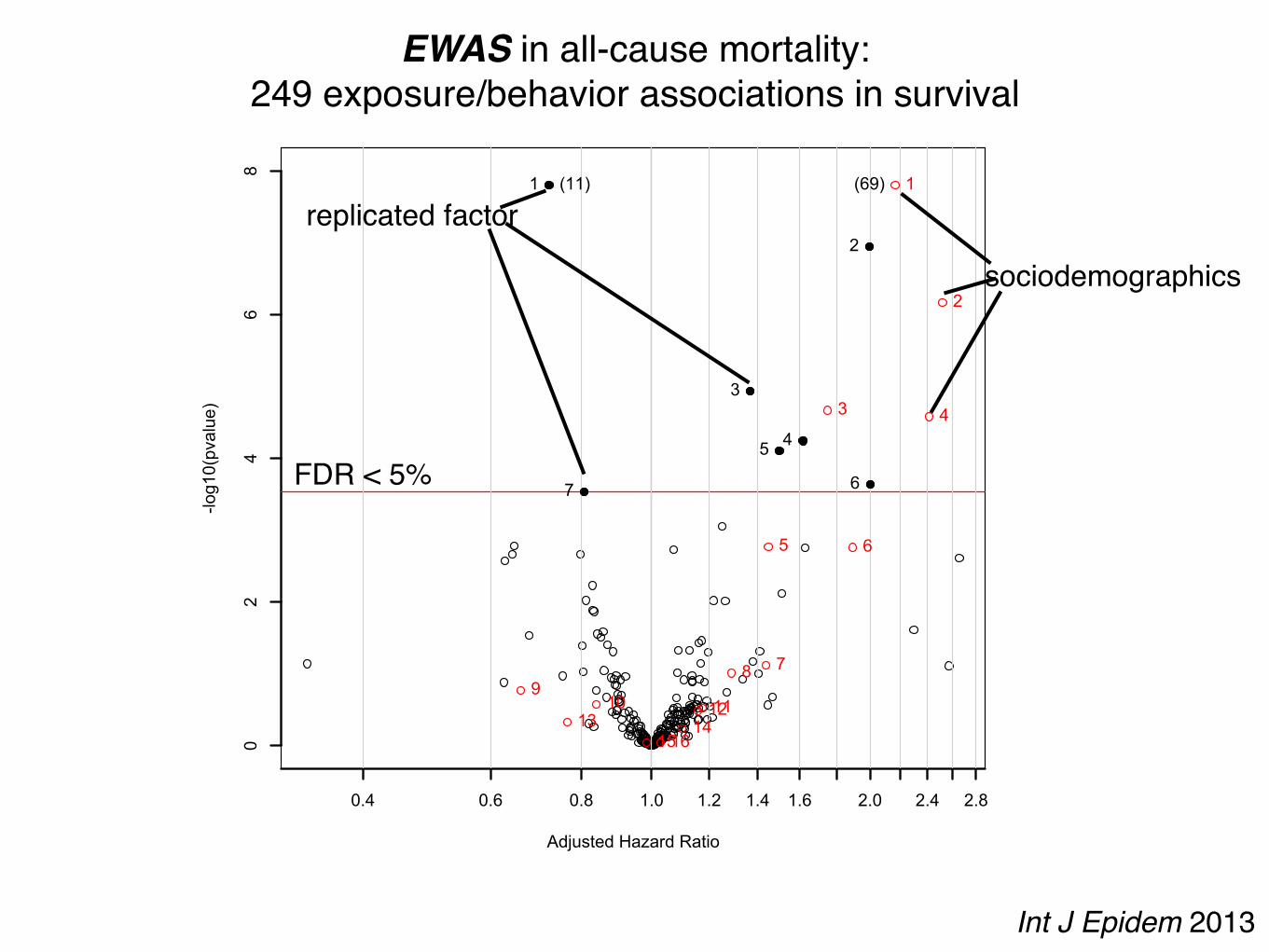
1 Physical Activity2 Does anyone smoke in home?3 Cadmium4 Cadmium, urine5 Past smoker6 Current smoker7 trans-lycopene
(11) 1
2
3 4
5 6
789
10 111213 141516
1 age (10 year increment)2 SES_13 male4 SES_05 black6 SES_27 SES_38 education_hs9 other_eth10 mexican11 occupation_blue_semi12 education_less_hs13 occupation_never14 occupation_blue_high15 occupation_white_semi16 other_hispanic
(69)
EWAS in all-cause mortality:249 exposure/behavior associations in survival
FDR < 5%
sociodemographics
replicated factor
Int J Epidem 2013

Adjusted Hazard Ratio
-log10(pvalue)
0.4 0.6 0.8 1.0 1.2 1.4 1.6 2.0 2.4 2.8
02
46
8
1
2
3
45
67
1 Physical Activity2 Does anyone smoke in home?3 Cadmium4 Cadmium, urine5 Past smoker6 Current smoker7 trans-lycopene
(11) 1
2
3 4
5 6
789
10 111213 141516
1 age (10 year increment)2 SES_13 male4 SES_05 black6 SES_27 SES_38 education_hs9 other_eth10 mexican11 occupation_blue_semi12 education_less_hs13 occupation_never14 occupation_blue_high15 occupation_white_semi16 other_hispanic
(69)
EWAS identifies factors associated with all-cause mortality:Volcano plot of 249 associations
age (10 years)
income (quintile 2)
income (quintile 1)male
black income (quintile 3)
any one smoke in home?
Multivariate cox (age, sex, income, education, race/ethnicity, occupation [in red])
serum and urine cadmium[1 SD]
past smoker?current smoker?serum lycopene
[1SD]
physical activity[low, moderate, high activity]*
*derived from METs per activity and categorized by Health.gov guidelines R2 ~ 2%
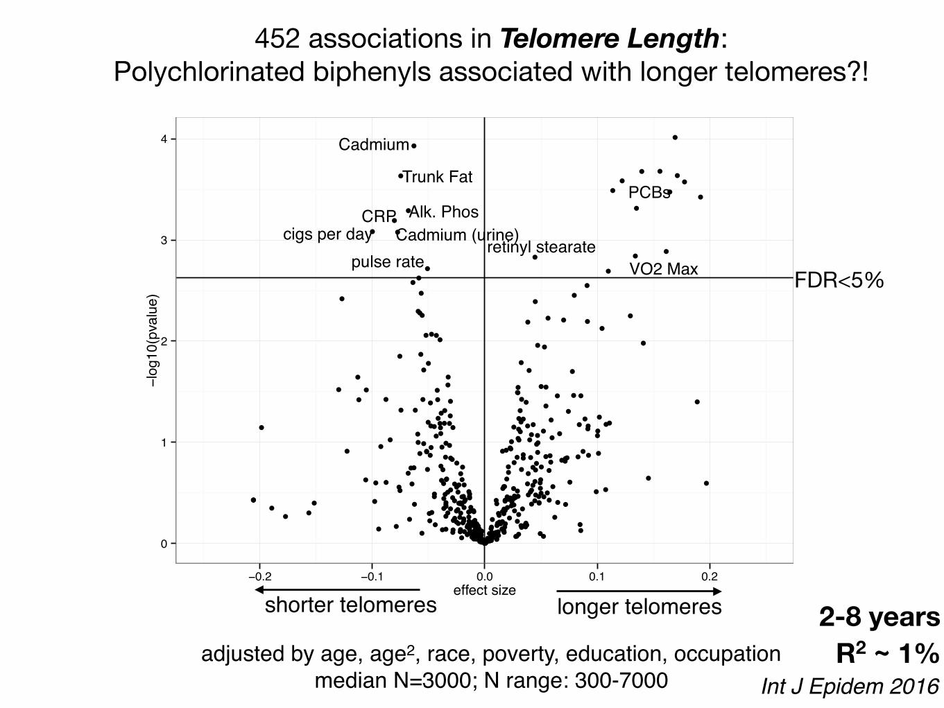
452 associations in Telomere Length: Polychlorinated biphenyls associated with longer telomeres?!
Int J Epidem 2016
0
1
2
3
4
−0.2 −0.1 0.0 0.1 0.2effect size
−log
10(p
valu
e)
PCBs
FDR<5%
Trunk Fat
Alk. PhosCRP
Cadmium
Cadmium (urine)cigs per dayretinyl stearate
R2 ~ 1%
VO2 Maxpulse rate
shorter telomeres longer telomeres
adjusted by age, age2, race, poverty, education, occupationmedian N=3000; N range: 300-7000
2-8 years
20 more examples:https://paperpile.com/shared/PtvEae
diabetespreterm birth
incomeblood pressure
lipidskidney diseasetelomere length
mortality

E+ E-
diseased
non-diseased
?
Versus
It is possible to capture E in high-throughput to create biomedical hypotheses using tools such as EWAS
candidates comprehensive
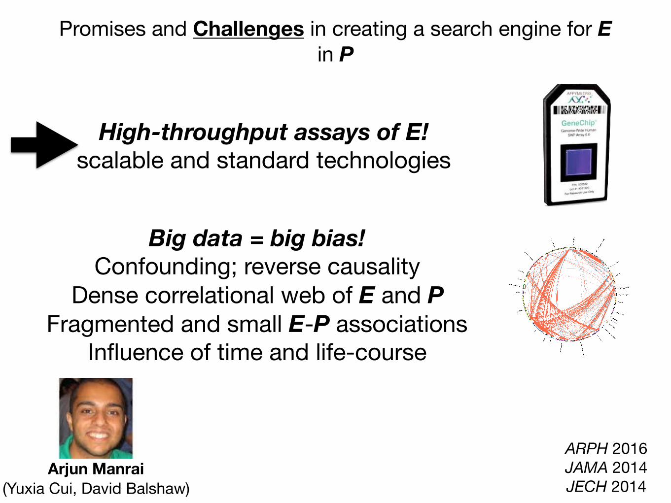
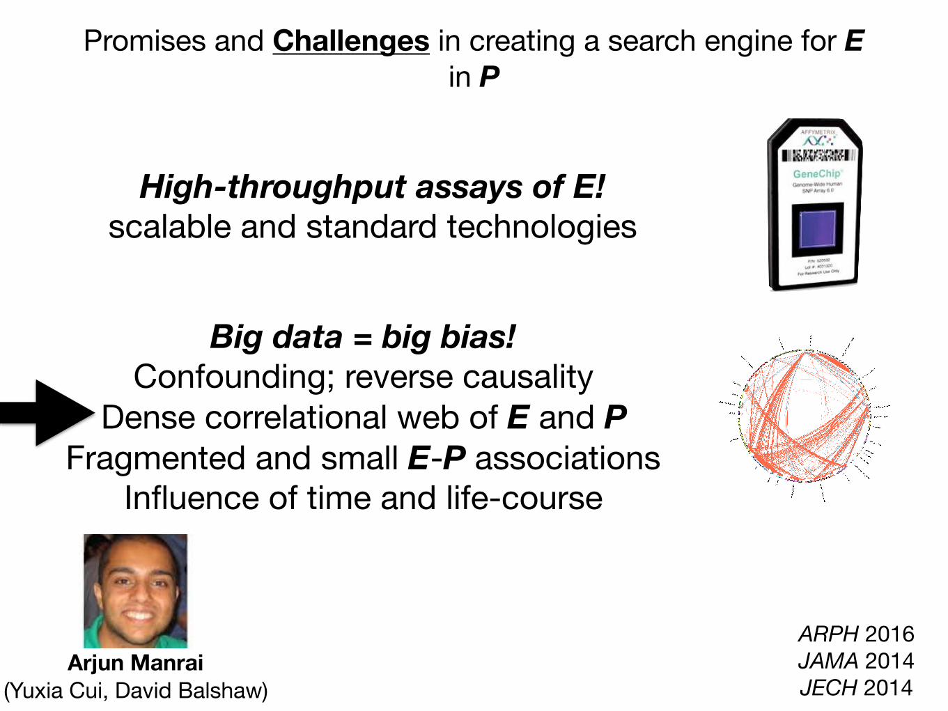
Promises and Challenges in creating a search engine for E in P
High-throughput assays of E!scalable and standard technologies
ARPH 2016JAMA 2014JECH 2014
Big data = big bias! Confounding; reverse causality
Dense correlational web of E and P Fragmented and small E-P associations
Influence of time and life-course
Arjun Manrai (Yuxia Cui, David Balshaw)

Challenge to scale absolute E due to heterogeneity and large dynamic range.
Rappaport et al, EHP 2015
Untargeted
Targeted

Promises and Challenges in creating a search engine for E in P
High-throughput assays of E!scalable and standard technologies
ARPH 2016JAMA 2014JECH 2014
Big data = big bias! Confounding; reverse causality
Dense correlational web of E and P Fragmented and small E-P associations
Influence of time and life-course
Arjun Manrai (Yuxia Cui, David Balshaw)
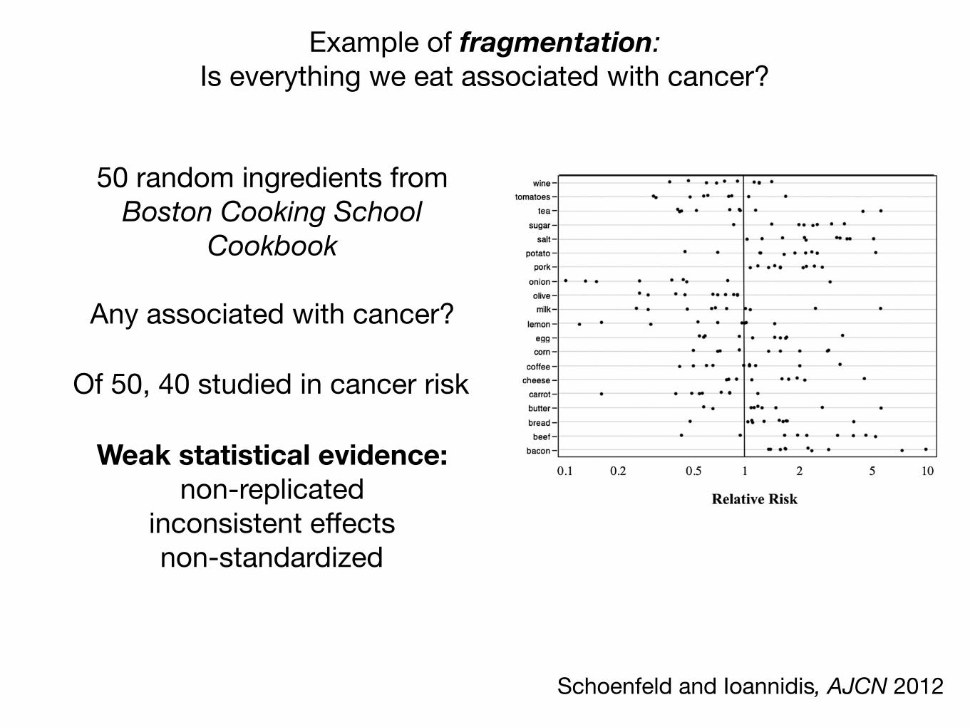
Example of fragmentation: Is everything we eat associated with cancer?
Schoenfeld and Ioannidis, AJCN 2012
50 random ingredients from Boston Cooking School
Cookbook
Any associated with cancer?
The effect estimates are shown in Figure 1 by malignancytype or by ingredient for the 20 ingredients for which $10 ar-ticles were identified. Gastrointestinal malignancies were themost commonly studied (45%), followed by genitourinary(14%), breast (14%), head and neck (9%), lung (5%), and gy-necologic (5%) malignancies.
The distribution of standardized (z) scores associated withP values was bimodal, with peaks corresponding to nominallystatistically significant results and a trough in the middle cor-responding to the sparse nonsignificant results (Figure 2, leftpanel). The bimodal peaks and middle trough pattern were evenmore prominent for results reported in the abstracts: 62% of thenominally statistically significant effect estimates were reported
in abstracts, whereas most (70%) of the nonsignificant resultsappeared only in the full text and not in the abstracts (P, 0.0001).
Meta-analyses
Thirty-six relevant effect estimates were obtained from meta-analyses (see Supplementary Table 2 under “Supplemental data”in the online issue). Author conclusions and the respective effectestimates are summarized in Table 1.
Thirty-three (92%) of the 36 estimates pertained to comparisonsof the lowest with the highest levels of consumption, but most ofthese meta-analyses combined studies that had different exposurecontrasts. For example, one meta-analysis (39) combined studies
FIGURE 1. Effect estimates reported in the literature by malignancy type (top) or ingredient (bottom). Only ingredients with$10 studies are shown. Threeoutliers are not shown (effect estimates .10).
4 of 8 SCHOENFELD AND IOANNIDIS
Of 50, 40 studied in cancer risk
Weak statistical evidence: non-replicated
inconsistent effectsnon-standardized

Are all the drugs we take associated with cancer?
Sci Reports 2016
Associated all (~500) drugs prescribed in entire population of Sweden(N=9M) with time to cancer
Assessed 2 modeling techniques (Cox and case-crossover)
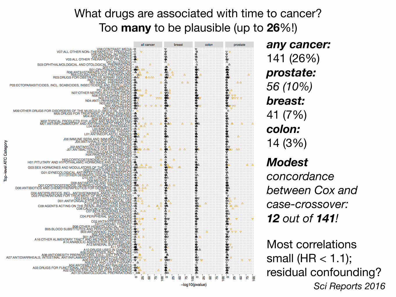
any cancer: 141 (26%)prostate: 56 (10%) breast: 41 (7%)colon: 14 (3%)
What drugs are associated with time to cancer?Too many to be plausible (up to 26%!)
Sci Reports 2016
Modest concordance between Cox and case-crossover: 12 out of 141!
Most correlations small (HR < 1.1); residual confounding?
Promises and Challenges in creating a search engine for E in P
High-throughput assays of E!scalable and standard technologies
ARPH 2016JAMA 2014JECH 2014
Big data = big bias! Confounding; reverse causality
Dense correlational web of E and P Fragmented and small E-P associations
Influence of time and life-course
Arjun Manrai (Yuxia Cui, David Balshaw)
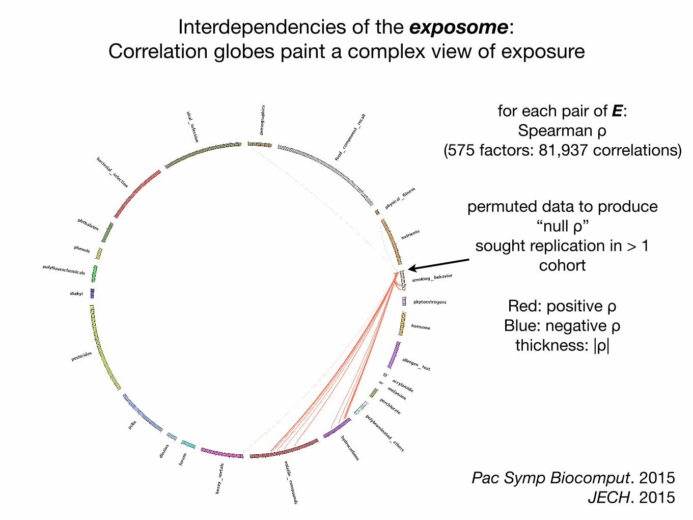
Interdependencies of the exposome: Correlation globes paint a complex view of exposure
Red: positive ρBlue: negative ρ
thickness: |ρ|
for each pair of E:Spearman ρ
(575 factors: 81,937 correlations)
permuted data to produce“null ρ”
sought replication in > 1 cohort
Pac Symp Biocomput. 2015JECH. 2015
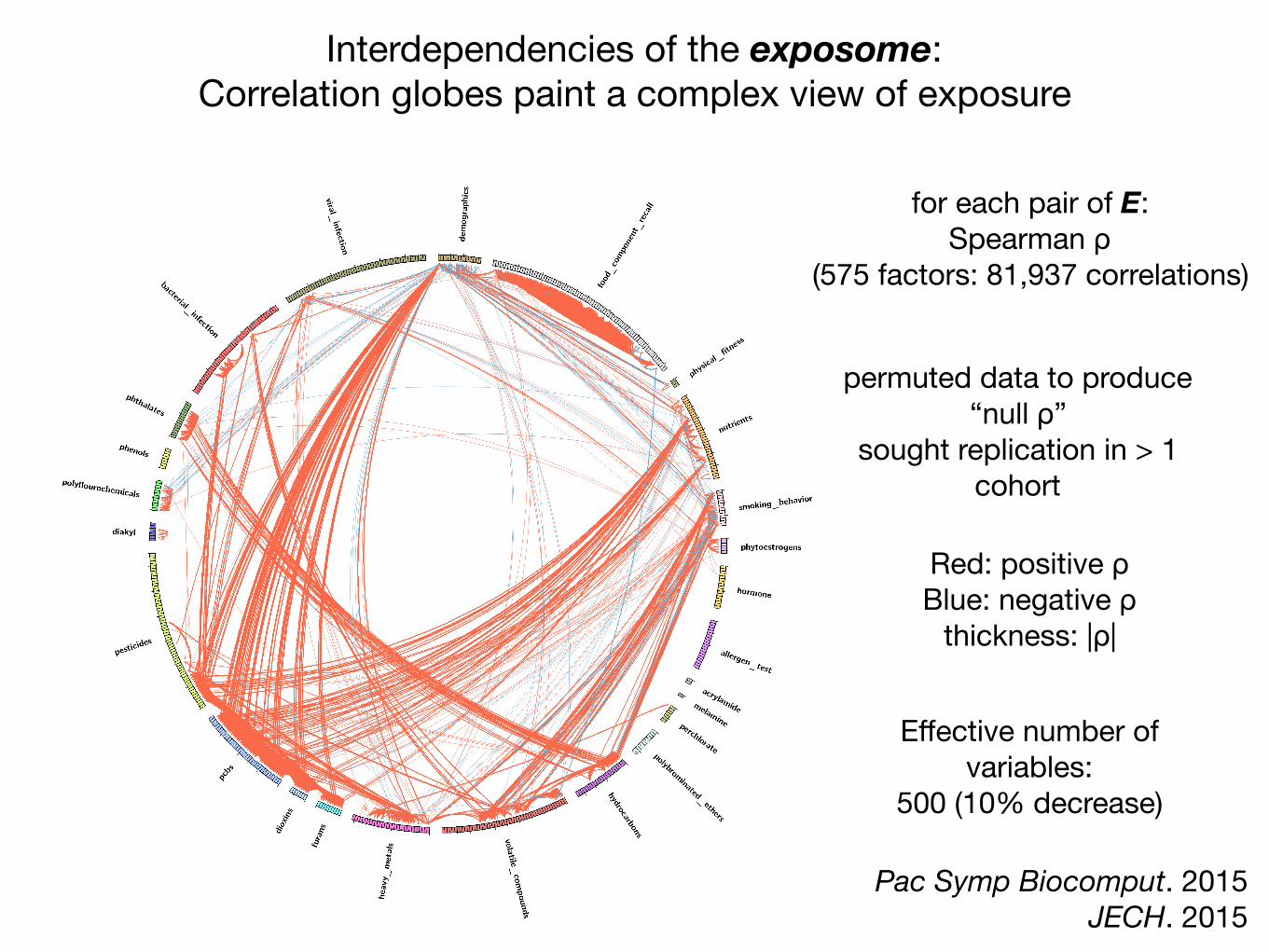
Red: positive ρBlue: negative ρ
thickness: |ρ|
for each pair of E:Spearman ρ
(575 factors: 81,937 correlations)
Interdependencies of the exposome: Correlation globes paint a complex view of exposure
permuted data to produce“null ρ”
sought replication in > 1 cohort
Pac Symp Biocomput. 2015JECH. 2015
Effective number of variables:
500 (10% decrease)
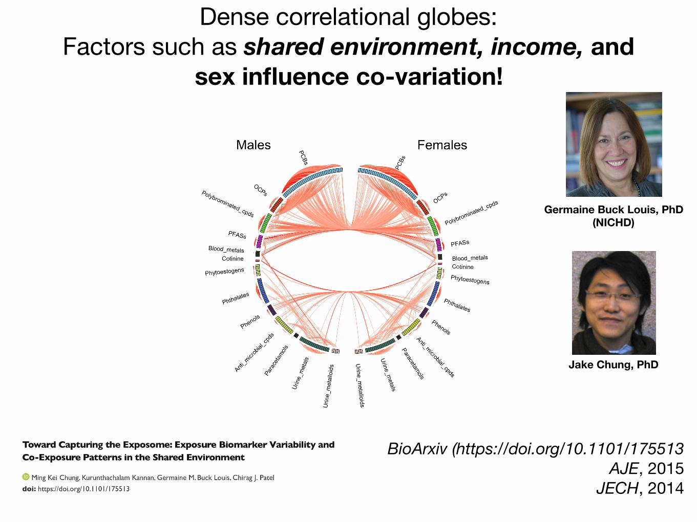
Dense correlational globes:Factors such as shared environment, income, and
sex influence co-variation!
BioArxiv (https://doi.org/10.1101/175513 AJE, 2015
JECH, 2014
Jake Chung, PhD
Germaine Buck Louis, PhD (NICHD)

Browse these and 82 other phenotype-exposome globes! http://www.chiragjpgroup.org/exposome_correlation

Does my single association between E and P matter?
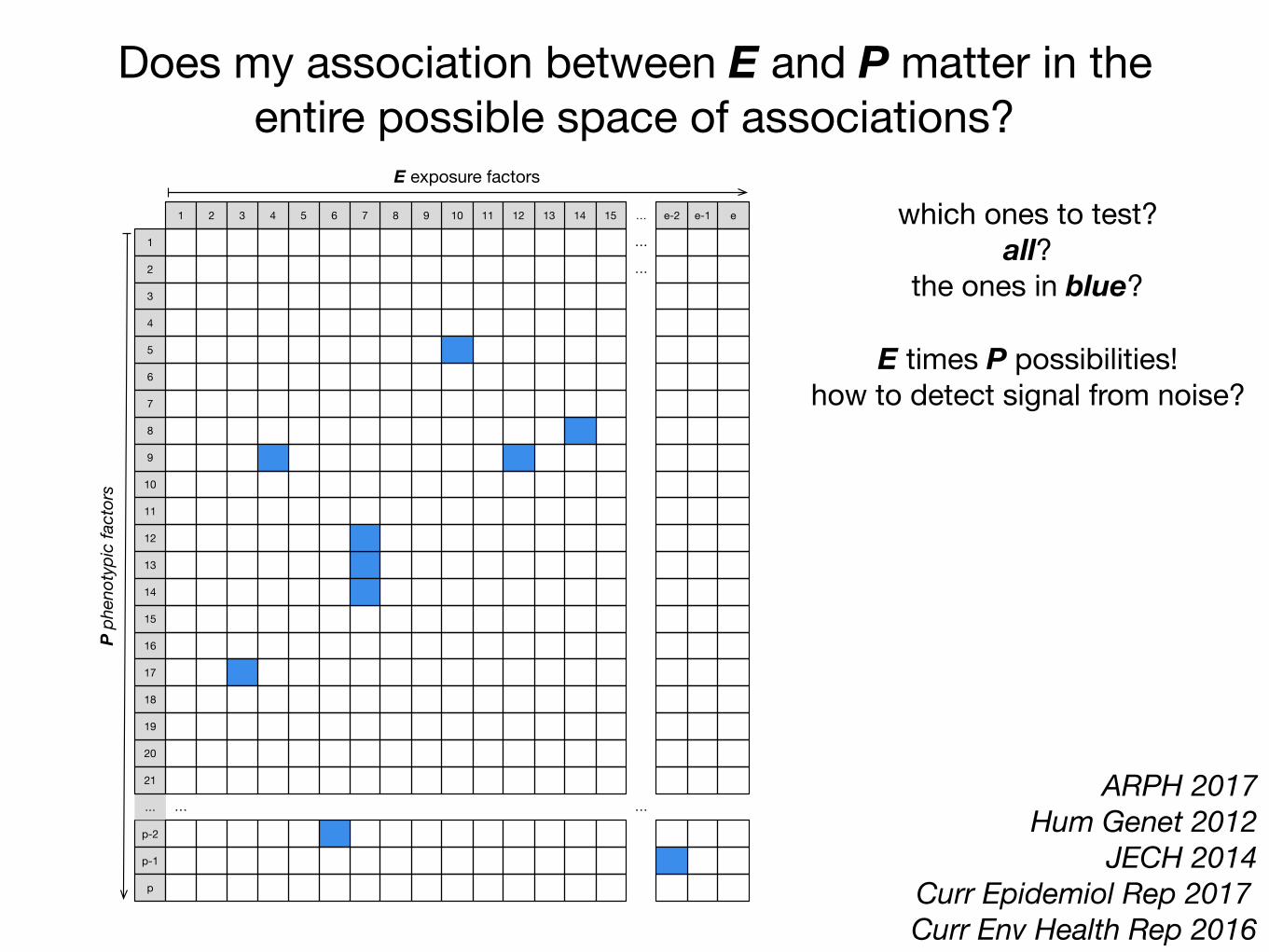
Does my association between E and P matter in the entire possible space of associations?
ARPH 2017 Hum Genet 2012
JECH 2014 Curr Epidemiol Rep 2017 Curr Env Health Rep 2016
p-2
20
8
1
6
18
7
10
…
p-1
12
2
5
9
4
16
21
11
13
3
17
14
19
p
15
6 101 1482 7 …1311 12 e54 153 9 e-1e-2
…
…
…
…
E exposure factors
P ph
enot
ypic
fact
ors
which ones to test?all?
the ones in blue?
E times P possibilities!how to detect signal from noise?
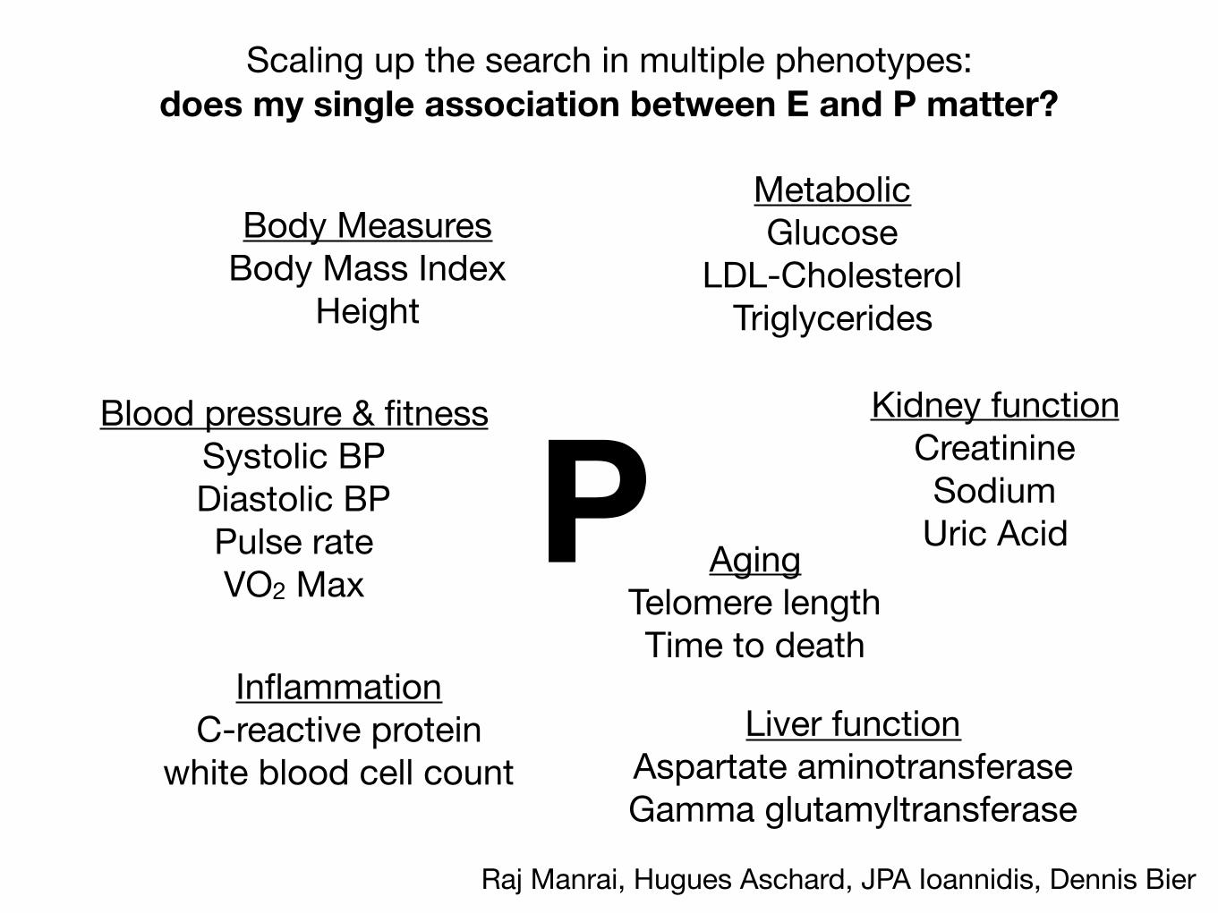
P
Scaling up the search in multiple phenotypes:does my single association between E and P matter?
Body MeasuresBody Mass Index
Height
Blood pressure & fitnessSystolic BPDiastolic BPPulse rateVO2 Max
MetabolicGlucose
LDL-CholesterolTriglycerides
InflammationC-reactive protein
white blood cell count
Kidney functionCreatinineSodium
Uric Acid
Liver functionAspartate aminotransferaseGamma glutamyltransferase
AgingTelomere lengthTime to death
Raj Manrai, Hugues Aschard, JPA Ioannidis, Dennis Bier

Creation of a phenotype-exposure association map: A 2-D view of 209 phenotype by 514 exposure associations
> 0< 0
Association Size:
504 E exposure and diet indicators × 209 clinical trait phenotypes NHANES 1999-2000, 2001-2002, 2005-2006, …, 2011-2012 (8)
Median N: 150-5000 per survey
~83,092 E-P associations! significant associations (FDR < 5%)
adjusted by age, age2, sex, race, income
Raj Manrai, Hugues Aschard, JPA Ioannidis, Dennis Bier
209
phe
noty
pes
514 exposures

83,092 total associations between E and P 12,237 significant associations (6%, in yellow):
Average association size: <1% for 1SD change in E
7%
percent change for 1 SD increase
-6%

Alpha-carotene
Alcohol
Vita
min
E a
s al
pha-
toco
pher
olBeta-carotene
Caffeine
Calcium
Carbohydrate
Cholesterol
Copper
Beta-cryptoxanthin
Folic
aci
dFo
late
, DFE
Food
fola
teD
ieta
ry fi
ber
Iron
Energy
Lycopene
Lute
in +
zea
xant
hin
MFA
16:
1M
FA 1
8:1
MFA
20:
1Magnesium
Tota
l mon
ouns
atur
ated
fatty
aci
dsMoisture
Niacin
PFA
18:
2P
FA 1
8:3
PFA
20:
4P
FA 2
2:5
PFA
22:
6To
tal p
olyu
nsat
urat
ed fa
tty a
cids
Phosphorus
Potassium
Protein
Retinol
SFA
4:0
SFA
6:0
SFA
8:0
SFA
10:
0S
FA 1
2:0
SFA
14:
0S
FA 1
6:0
SFA
18:
0Selenium
Tota
l sat
urat
ed fa
tty a
cids
Tota
l sug
ars
Tota
l fat
Theobromine
Vita
min
A, R
AE
Thiamin
Vita
min
B12
Riboflavin
Vita
min
B6
Vita
min
CV
itam
in K
Zinc
No
Sal
tO
rdin
ary
Sal
ta-Carotene
Vita
min
B12
, ser
umtrans-b-carotene
cis-b-carotene
b-cryptoxanthin
Fola
te, s
erum
g-tocopherol
Iron,
Fro
zen
Ser
umC
ombi
ned
Lute
in/z
eaxa
nthi
ntrans-lycopene
Fola
te, R
BC
Ret
inyl
pal
mita
teR
etin
yl s
tear
ate
Retinol
Vita
min
Da-Tocopherol
Daidzein
o-Desmethylangolensin
Equol
Enterodiol
Enterolactone
Genistein
Est
imat
ed V
O2m
axP
hysi
cal A
ctiv
ityD
oes
anyo
ne s
mok
e in
hom
e?To
tal #
of c
igar
ette
s sm
oked
in h
ome
Cotinine
Cur
rent
Cig
aret
te S
mok
er?
Age
last
sm
oked
cig
aret
tes
regu
larly
# ci
gare
ttes
smok
ed p
er d
ay w
hen
quit
# ci
gare
ttes
smok
ed p
er d
ay n
ow#
days
sm
oked
cig
s du
ring
past
30
days
Avg
# c
igar
ette
s/da
y du
ring
past
30
days
Sm
oked
at l
east
100
cig
aret
tes
in li
feD
o yo
u no
w s
mok
e ci
gare
ttes.
..nu
mbe
r of d
ays
sinc
e qu
itU
sed
snuf
f at l
east
20
times
in li
fedr
ink
5 in
a d
aydr
ink
per d
ayda
ys 5
drin
ks in
yea
rda
ys d
rink
in y
ear
3-fluorene
2-fluorene
3-phenanthrene
1-phenanthrene
2-phenanthrene
1-pyrene
3-be
nzo[
c] p
hena
nthr
ene
3-be
nz[a
] ant
hrac
ene
Mon
o-n-
buty
l pht
hala
teM
ono-
pht
hala
teM
ono-
cycl
ohex
yl p
htha
late
Mon
o-et
hyl p
htha
late
Mon
o- p
htha
late
Mon
o--h
exyl
pht
hala
teM
ono-
isob
utyl
pht
hala
teM
ono-
n-m
ethy
l pht
hala
teM
ono-
pht
hala
teM
ono-
benz
yl p
htha
late
Cadmium
Lead
Mer
cury
, tot
alB
ariu
m, u
rine
Cad
miu
m, u
rine
Cob
alt,
urin
eC
esiu
m, u
rine
Mer
cury
, urin
eIo
dine
, urin
eM
olyb
denu
m, u
rine
Lead
, urin
eP
latin
um, u
rine
Ant
imon
y, u
rine
Thal
lium
, urin
eTu
ngst
en, u
rine
Ura
nium
, urin
eB
lood
Ben
zene
Blo
od E
thyl
benz
ene
Blo
od o
-Xyl
ene
Blo
od S
tyre
neB
lood
Tric
hlor
oeth
ene
Blo
od T
olue
neB
lood
m-/p
-Xyl
ene
1,2,3,7,8-pncdd
1,2,3,7,8,9-hxcdd
1,2,3,4,6,7,8-hpcdd
1,2,3,4,6,7,8,9-ocdd
2,3,7,8-tcdd
Beta-hexachlorocyclohexane
Gamma-hexachlorocyclohexane
Hexachlorobenzene
Hep
tach
lor E
poxi
deMirex
Oxychlordane
p,p-DDE
Trans-nonachlor
2,5-
dich
loro
phen
ol re
sult
2,4,
6-tri
chlo
roph
enol
resu
ltPentachlorophenol
Dimethylphosphate
Diethylphosphate
Dimethylthiophosphate
PCB66
PCB74
PCB99
PCB105
PCB118
PC
B13
8 &
158
PCB146
PCB153
PCB156
PCB157
PCB167
PCB170
PCB172
PCB177
PCB178
PCB180
PCB183
PCB187
3,3,4,4,5,5-hxcb
3,3,4,4,5-pncb
3,4,4,5-tcb
Per
fluor
ohep
tano
ic a
cid
Per
fluor
ohex
ane
sulfo
nic
acid
Per
fluor
onon
anoi
c ac
idP
erflu
oroo
ctan
oic
acid
Per
fluor
ooct
ane
sulfo
nic
acid
Per
fluor
ooct
ane
sulfo
nam
ide
2,3,7,8-tcdf
1,2,3,7,8-pncdf
2,3,4,7,8-pncdf
1,2,3,4,7,8-hxcdf
1,2,3,6,7,8-hxcdf
1,2,3,7,8,9-hxcdf
2,3,4,6,7,8-hxcdf
1,2,3,4,6,7,8-hpcdf
Measles
Toxoplasma
Hep
atiti
s A
Ant
ibod
yH
epat
itis
B c
ore
antib
ody
Hep
atiti
s B
Sur
face
Ant
ibod
yH
erpe
s II
Albumin, urineUric acidPhosphorusOsmolalitySodiumPotassiumCreatinineChlorideTotal calciumBicarbonateBlood urea nitrogenTotal proteinTotal bilirubinLactate dehydrogenase LDHGamma glutamyl transferaseGlobulinAlanine aminotransferase ALTAspartate aminotransferase ASTAlkaline phosphotaseAlbuminMethylmalonic acidPSA. totalProstate specific antigen ratioTIBC, Frozen SerumRed cell distribution widthRed blood cell countPlatelet count SISegmented neutrophils percentMean platelet volumeMean cell volumeMean cell hemoglobinMCHCHemoglobinHematocritFerritinProtoporphyrinTransferrin saturationWhite blood cell countMonocyte percentLymphocyte percentEosinophils percentC-reactive proteinSegmented neutrophils numberMonocyte numberLymphocyte numberEosinophils numberBasophils numbermean systolicmean diastolic60 sec. pulse:60 sec HRTotal CholesterolTriglyceridesGlucose, serumInsulinHomocysteineGlucose, plasmaGlycohemoglobinC-peptide: SILDL-cholesterolDirect HDL-CholesterolBone alkaline phosphotaseTrunk FatLumber Pelvis BMDLumber Spine BMDHead BMDTrunk Lean excl BMCTotal Lean excl BMCTotal FatTotal BMDWeightWaist CircumferenceTriceps SkinfoldThigh CircumferenceSubscapular SkinfoldRecumbent LengthUpper Leg LengthStanding HeightHead CircumferenceMaximal Calf CircumferenceBody Mass Index
-0.4 -0.2 0 0.2 0.4
Value
050
100
150
Color Keyand Histogram
Count
phen
otyp
es
exposures
+- EWAS-derived phenotype-exposure association map: A 2-D view of connections between P and E

Alpha-carotene
Alcohol
Vita
min
E a
s al
pha-
toco
pher
olBeta-carotene
Caffeine
Calcium
Carbohydrate
Cholesterol
Copper
Beta-cryptoxanthin
Folic
aci
dFo
late
, DFE
Food
fola
teD
ieta
ry fi
ber
Iron
Energy
Lycopene
Lute
in +
zea
xant
hin
MFA
16:
1M
FA 1
8:1
MFA
20:
1Magnesium
Tota
l mon
ouns
atur
ated
fatty
aci
dsMoisture
Niacin
PFA
18:
2P
FA 1
8:3
PFA
20:
4P
FA 2
2:5
PFA
22:
6To
tal p
olyu
nsat
urat
ed fa
tty a
cids
Phosphorus
Potassium
Protein
Retinol
SFA
4:0
SFA
6:0
SFA
8:0
SFA
10:
0S
FA 1
2:0
SFA
14:
0S
FA 1
6:0
SFA
18:
0Selenium
Tota
l sat
urat
ed fa
tty a
cids
Tota
l sug
ars
Tota
l fat
Theobromine
Vita
min
A, R
AE
Thiamin
Vita
min
B12
Riboflavin
Vita
min
B6
Vita
min
CV
itam
in K
Zinc
No
Sal
tO
rdin
ary
Sal
ta-Carotene
Vita
min
B12
, ser
umtrans-b-carotene
cis-b-carotene
b-cryptoxanthin
Fola
te, s
erum
g-tocopherol
Iron,
Fro
zen
Ser
umC
ombi
ned
Lute
in/z
eaxa
nthi
ntrans-lycopene
Fola
te, R
BC
Ret
inyl
pal
mita
teR
etin
yl s
tear
ate
Retinol
Vita
min
Da-Tocopherol
Daidzein
o-Desmethylangolensin
Equol
Enterodiol
Enterolactone
Genistein
Est
imat
ed V
O2m
axP
hysi
cal A
ctiv
ityD
oes
anyo
ne s
mok
e in
hom
e?To
tal #
of c
igar
ette
s sm
oked
in h
ome
Cotinine
Cur
rent
Cig
aret
te S
mok
er?
Age
last
sm
oked
cig
aret
tes
regu
larly
# ci
gare
ttes
smok
ed p
er d
ay w
hen
quit
# ci
gare
ttes
smok
ed p
er d
ay n
ow#
days
sm
oked
cig
s du
ring
past
30
days
Avg
# c
igar
ette
s/da
y du
ring
past
30
days
Sm
oked
at l
east
100
cig
aret
tes
in li
feD
o yo
u no
w s
mok
e ci
gare
ttes.
..nu
mbe
r of d
ays
sinc
e qu
itU
sed
snuf
f at l
east
20
times
in li
fedr
ink
5 in
a d
aydr
ink
per d
ayda
ys 5
drin
ks in
yea
rda
ys d
rink
in y
ear
3-fluorene
2-fluorene
3-phenanthrene
1-phenanthrene
2-phenanthrene
1-pyrene
3-be
nzo[
c] p
hena
nthr
ene
3-be
nz[a
] ant
hrac
ene
Mon
o-n-
buty
l pht
hala
teM
ono-
pht
hala
teM
ono-
cycl
ohex
yl p
htha
late
Mon
o-et
hyl p
htha
late
Mon
o- p
htha
late
Mon
o--h
exyl
pht
hala
teM
ono-
isob
utyl
pht
hala
teM
ono-
n-m
ethy
l pht
hala
teM
ono-
pht
hala
teM
ono-
benz
yl p
htha
late
Cadmium
Lead
Mer
cury
, tot
alB
ariu
m, u
rine
Cad
miu
m, u
rine
Cob
alt,
urin
eC
esiu
m, u
rine
Mer
cury
, urin
eIo
dine
, urin
eM
olyb
denu
m, u
rine
Lead
, urin
eP
latin
um, u
rine
Ant
imon
y, u
rine
Thal
lium
, urin
eTu
ngst
en, u
rine
Ura
nium
, urin
eB
lood
Ben
zene
Blo
od E
thyl
benz
ene
Blo
od o
-Xyl
ene
Blo
od S
tyre
neB
lood
Tric
hlor
oeth
ene
Blo
od T
olue
neB
lood
m-/p
-Xyl
ene
1,2,3,7,8-pncdd
1,2,3,7,8,9-hxcdd
1,2,3,4,6,7,8-hpcdd
1,2,3,4,6,7,8,9-ocdd
2,3,7,8-tcdd
Beta-hexachlorocyclohexane
Gamma-hexachlorocyclohexane
Hexachlorobenzene
Hep
tach
lor E
poxi
deMirex
Oxychlordane
p,p-DDE
Trans-nonachlor
2,5-
dich
loro
phen
ol re
sult
2,4,
6-tri
chlo
roph
enol
resu
ltPentachlorophenol
Dimethylphosphate
Diethylphosphate
Dimethylthiophosphate
PCB66
PCB74
PCB99
PCB105
PCB118
PC
B13
8 &
158
PCB146
PCB153
PCB156
PCB157
PCB167
PCB170
PCB172
PCB177
PCB178
PCB180
PCB183
PCB187
3,3,4,4,5,5-hxcb
3,3,4,4,5-pncb
3,4,4,5-tcb
Per
fluor
ohep
tano
ic a
cid
Per
fluor
ohex
ane
sulfo
nic
acid
Per
fluor
onon
anoi
c ac
idP
erflu
oroo
ctan
oic
acid
Per
fluor
ooct
ane
sulfo
nic
acid
Per
fluor
ooct
ane
sulfo
nam
ide
2,3,7,8-tcdf
1,2,3,7,8-pncdf
2,3,4,7,8-pncdf
1,2,3,4,7,8-hxcdf
1,2,3,6,7,8-hxcdf
1,2,3,7,8,9-hxcdf
2,3,4,6,7,8-hxcdf
1,2,3,4,6,7,8-hpcdf
Measles
Toxoplasma
Hep
atiti
s A
Ant
ibod
yH
epat
itis
B c
ore
antib
ody
Hep
atiti
s B
Sur
face
Ant
ibod
yH
erpe
s II
Albumin, urineUric acidPhosphorusOsmolalitySodiumPotassiumCreatinineChlorideTotal calciumBicarbonateBlood urea nitrogenTotal proteinTotal bilirubinLactate dehydrogenase LDHGamma glutamyl transferaseGlobulinAlanine aminotransferase ALTAspartate aminotransferase ASTAlkaline phosphotaseAlbuminMethylmalonic acidPSA. totalProstate specific antigen ratioTIBC, Frozen SerumRed cell distribution widthRed blood cell countPlatelet count SISegmented neutrophils percentMean platelet volumeMean cell volumeMean cell hemoglobinMCHCHemoglobinHematocritFerritinProtoporphyrinTransferrin saturationWhite blood cell countMonocyte percentLymphocyte percentEosinophils percentC-reactive proteinSegmented neutrophils numberMonocyte numberLymphocyte numberEosinophils numberBasophils numbermean systolicmean diastolic60 sec. pulse:60 sec HRTotal CholesterolTriglyceridesGlucose, serumInsulinHomocysteineGlucose, plasmaGlycohemoglobinC-peptide: SILDL-cholesterolDirect HDL-CholesterolBone alkaline phosphotaseTrunk FatLumber Pelvis BMDLumber Spine BMDHead BMDTrunk Lean excl BMCTotal Lean excl BMCTotal FatTotal BMDWeightWaist CircumferenceTriceps SkinfoldThigh CircumferenceSubscapular SkinfoldRecumbent LengthUpper Leg LengthStanding HeightHead CircumferenceMaximal Calf CircumferenceBody Mass Index
-0.4 -0.2 0 0.2 0.4
Value
050
100
150
Color Keyand Histogram
Count
phen
otyp
es
exposures
+-
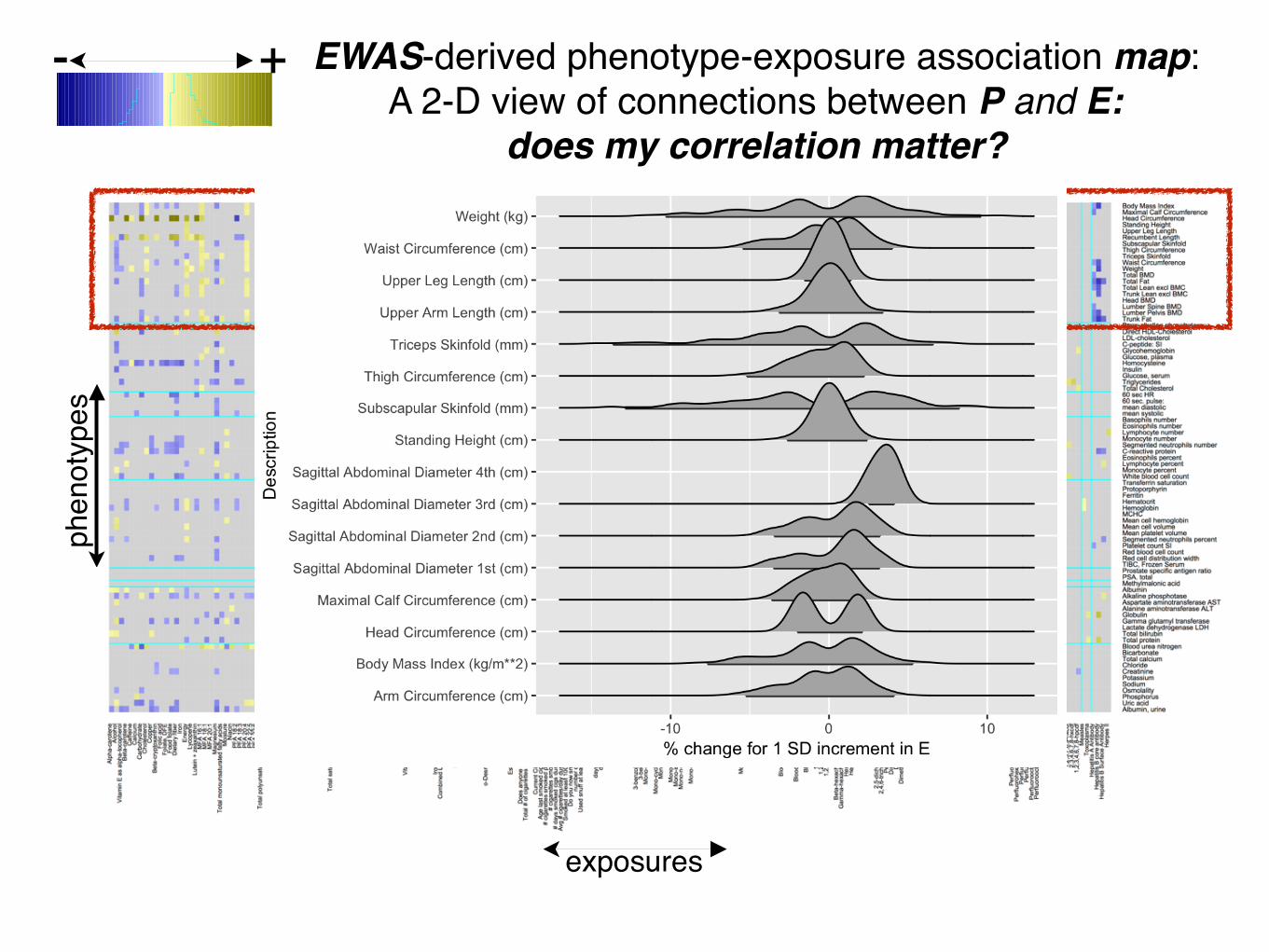
nutrients
BMI,
wei
ght,
BMD
met
abol
ic
rena
l fun
ctio
npcbs
met
abol
ic
bloo
d pa
ram
eter
s
hydrocarbons
EWAS-derived phenotype-exposure association map: A 2-D view of connections between P and E
R2: ~1-40% (average of 20%)

Alpha-carotene
Alcohol
Vita
min
E a
s al
pha-
toco
pher
olBeta-carotene
Caffeine
Calcium
Carbohydrate
Cholesterol
Copper
Beta-cryptoxanthin
Folic
aci
dFo
late
, DFE
Food
fola
teD
ieta
ry fi
ber
Iron
Energy
Lycopene
Lute
in +
zea
xant
hin
MFA
16:
1M
FA 1
8:1
MFA
20:
1Magnesium
Tota
l mon
ouns
atur
ated
fatty
aci
dsMoisture
Niacin
PFA
18:
2P
FA 1
8:3
PFA
20:
4P
FA 2
2:5
PFA
22:
6To
tal p
olyu
nsat
urat
ed fa
tty a
cids
Phosphorus
Potassium
Protein
Retinol
SFA
4:0
SFA
6:0
SFA
8:0
SFA
10:
0S
FA 1
2:0
SFA
14:
0S
FA 1
6:0
SFA
18:
0Selenium
Tota
l sat
urat
ed fa
tty a
cids
Tota
l sug
ars
Tota
l fat
Theobromine
Vita
min
A, R
AE
Thiamin
Vita
min
B12
Riboflavin
Vita
min
B6
Vita
min
CV
itam
in K
Zinc
No
Sal
tO
rdin
ary
Sal
ta-Carotene
Vita
min
B12
, ser
umtrans-b-carotene
cis-b-carotene
b-cryptoxanthin
Fola
te, s
erum
g-tocopherol
Iron,
Fro
zen
Ser
umC
ombi
ned
Lute
in/z
eaxa
nthi
ntrans-lycopene
Fola
te, R
BC
Ret
inyl
pal
mita
teR
etin
yl s
tear
ate
Retinol
Vita
min
Da-Tocopherol
Daidzein
o-Desmethylangolensin
Equol
Enterodiol
Enterolactone
Genistein
Est
imat
ed V
O2m
axP
hysi
cal A
ctiv
ityD
oes
anyo
ne s
mok
e in
hom
e?To
tal #
of c
igar
ette
s sm
oked
in h
ome
Cotinine
Cur
rent
Cig
aret
te S
mok
er?
Age
last
sm
oked
cig
aret
tes
regu
larly
# ci
gare
ttes
smok
ed p
er d
ay w
hen
quit
# ci
gare
ttes
smok
ed p
er d
ay n
ow#
days
sm
oked
cig
s du
ring
past
30
days
Avg
# c
igar
ette
s/da
y du
ring
past
30
days
Sm
oked
at l
east
100
cig
aret
tes
in li
feD
o yo
u no
w s
mok
e ci
gare
ttes.
..nu
mbe
r of d
ays
sinc
e qu
itU
sed
snuf
f at l
east
20
times
in li
fedr
ink
5 in
a d
aydr
ink
per d
ayda
ys 5
drin
ks in
yea
rda
ys d
rink
in y
ear
3-fluorene
2-fluorene
3-phenanthrene
1-phenanthrene
2-phenanthrene
1-pyrene
3-be
nzo[
c] p
hena
nthr
ene
3-be
nz[a
] ant
hrac
ene
Mon
o-n-
buty
l pht
hala
teM
ono-
pht
hala
teM
ono-
cycl
ohex
yl p
htha
late
Mon
o-et
hyl p
htha
late
Mon
o- p
htha
late
Mon
o--h
exyl
pht
hala
teM
ono-
isob
utyl
pht
hala
teM
ono-
n-m
ethy
l pht
hala
teM
ono-
pht
hala
teM
ono-
benz
yl p
htha
late
Cadmium
Lead
Mer
cury
, tot
alB
ariu
m, u
rine
Cad
miu
m, u
rine
Cob
alt,
urin
eC
esiu
m, u
rine
Mer
cury
, urin
eIo
dine
, urin
eM
olyb
denu
m, u
rine
Lead
, urin
eP
latin
um, u
rine
Ant
imon
y, u
rine
Thal
lium
, urin
eTu
ngst
en, u
rine
Ura
nium
, urin
eB
lood
Ben
zene
Blo
od E
thyl
benz
ene
Blo
od o
-Xyl
ene
Blo
od S
tyre
neB
lood
Tric
hlor
oeth
ene
Blo
od T
olue
neB
lood
m-/p
-Xyl
ene
1,2,3,7,8-pncdd
1,2,3,7,8,9-hxcdd
1,2,3,4,6,7,8-hpcdd
1,2,3,4,6,7,8,9-ocdd
2,3,7,8-tcdd
Beta-hexachlorocyclohexane
Gamma-hexachlorocyclohexane
Hexachlorobenzene
Hep
tach
lor E
poxi
deMirex
Oxychlordane
p,p-DDE
Trans-nonachlor
2,5-
dich
loro
phen
ol re
sult
2,4,
6-tri
chlo
roph
enol
resu
ltPentachlorophenol
Dimethylphosphate
Diethylphosphate
Dimethylthiophosphate
PCB66
PCB74
PCB99
PCB105
PCB118
PC
B13
8 &
158
PCB146
PCB153
PCB156
PCB157
PCB167
PCB170
PCB172
PCB177
PCB178
PCB180
PCB183
PCB187
3,3,4,4,5,5-hxcb
3,3,4,4,5-pncb
3,4,4,5-tcb
Per
fluor
ohep
tano
ic a
cid
Per
fluor
ohex
ane
sulfo
nic
acid
Per
fluor
onon
anoi
c ac
idP
erflu
oroo
ctan
oic
acid
Per
fluor
ooct
ane
sulfo
nic
acid
Per
fluor
ooct
ane
sulfo
nam
ide
2,3,7,8-tcdf
1,2,3,7,8-pncdf
2,3,4,7,8-pncdf
1,2,3,4,7,8-hxcdf
1,2,3,6,7,8-hxcdf
1,2,3,7,8,9-hxcdf
2,3,4,6,7,8-hxcdf
1,2,3,4,6,7,8-hpcdf
Measles
Toxoplasma
Hep
atiti
s A
Ant
ibod
yH
epat
itis
B c
ore
antib
ody
Hep
atiti
s B
Sur
face
Ant
ibod
yH
erpe
s II
Albumin, urineUric acidPhosphorusOsmolalitySodiumPotassiumCreatinineChlorideTotal calciumBicarbonateBlood urea nitrogenTotal proteinTotal bilirubinLactate dehydrogenase LDHGamma glutamyl transferaseGlobulinAlanine aminotransferase ALTAspartate aminotransferase ASTAlkaline phosphotaseAlbuminMethylmalonic acidPSA. totalProstate specific antigen ratioTIBC, Frozen SerumRed cell distribution widthRed blood cell countPlatelet count SISegmented neutrophils percentMean platelet volumeMean cell volumeMean cell hemoglobinMCHCHemoglobinHematocritFerritinProtoporphyrinTransferrin saturationWhite blood cell countMonocyte percentLymphocyte percentEosinophils percentC-reactive proteinSegmented neutrophils numberMonocyte numberLymphocyte numberEosinophils numberBasophils numbermean systolicmean diastolic60 sec. pulse:60 sec HRTotal CholesterolTriglyceridesGlucose, serumInsulinHomocysteineGlucose, plasmaGlycohemoglobinC-peptide: SILDL-cholesterolDirect HDL-CholesterolBone alkaline phosphotaseTrunk FatLumber Pelvis BMDLumber Spine BMDHead BMDTrunk Lean excl BMCTotal Lean excl BMCTotal FatTotal BMDWeightWaist CircumferenceTriceps SkinfoldThigh CircumferenceSubscapular SkinfoldRecumbent LengthUpper Leg LengthStanding HeightHead CircumferenceMaximal Calf CircumferenceBody Mass Index
-0.4 -0.2 0 0.2 0.4
Value
050
100
150
Color Keyand Histogram
Count
phen
otyp
es
exposures
+- EWAS-derived phenotype-exposure association map: A 2-D view of connections between P and E:
does my correlation matter?
EWAS-derived phenotype-exposure association map: A 2-D view of connections between P and E:
does my correlation matter?
Alpha-carotene
Alcohol
Vita
min
E a
s al
pha-
toco
pher
olBeta-carotene
Caffeine
Calcium
Carbohydrate
Cholesterol
Copper
Beta-cryptoxanthin
Folic
aci
dFo
late
, DFE
Food
fola
teD
ieta
ry fi
ber
Iron
Energy
Lycopene
Lute
in +
zea
xant
hin
MFA
16:
1M
FA 1
8:1
MFA
20:
1Magnesium
Tota
l mon
ouns
atur
ated
fatty
aci
dsMoisture
Niacin
PFA
18:
2P
FA 1
8:3
PFA
20:
4P
FA 2
2:5
PFA
22:
6To
tal p
olyu
nsat
urat
ed fa
tty a
cids
Phosphorus
Potassium
Protein
Retinol
SFA
4:0
SFA
6:0
SFA
8:0
SFA
10:
0S
FA 1
2:0
SFA
14:
0S
FA 1
6:0
SFA
18:
0Selenium
Tota
l sat
urat
ed fa
tty a
cids
Tota
l sug
ars
Tota
l fat
Theobromine
Vita
min
A, R
AE
Thiamin
Vita
min
B12
Riboflavin
Vita
min
B6
Vita
min
CV
itam
in K
Zinc
No
Sal
tO
rdin
ary
Sal
ta-Carotene
Vita
min
B12
, ser
umtrans-b-carotene
cis-b-carotene
b-cryptoxanthin
Fola
te, s
erum
g-tocopherol
Iron,
Fro
zen
Ser
umC
ombi
ned
Lute
in/z
eaxa
nthi
ntrans-lycopene
Fola
te, R
BC
Ret
inyl
pal
mita
teR
etin
yl s
tear
ate
Retinol
Vita
min
Da-Tocopherol
Daidzein
o-Desmethylangolensin
Equol
Enterodiol
Enterolactone
Genistein
Est
imat
ed V
O2m
axP
hysi
cal A
ctiv
ityD
oes
anyo
ne s
mok
e in
hom
e?To
tal #
of c
igar
ette
s sm
oked
in h
ome
Cotinine
Cur
rent
Cig
aret
te S
mok
er?
Age
last
sm
oked
cig
aret
tes
regu
larly
# ci
gare
ttes
smok
ed p
er d
ay w
hen
quit
# ci
gare
ttes
smok
ed p
er d
ay n
ow#
days
sm
oked
cig
s du
ring
past
30
days
Avg
# c
igar
ette
s/da
y du
ring
past
30
days
Sm
oked
at l
east
100
cig
aret
tes
in li
feD
o yo
u no
w s
mok
e ci
gare
ttes.
..nu
mbe
r of d
ays
sinc
e qu
itU
sed
snuf
f at l
east
20
times
in li
fedr
ink
5 in
a d
aydr
ink
per d
ayda
ys 5
drin
ks in
yea
rda
ys d
rink
in y
ear
3-fluorene
2-fluorene
3-phenanthrene
1-phenanthrene
2-phenanthrene
1-pyrene
3-be
nzo[
c] p
hena
nthr
ene
3-be
nz[a
] ant
hrac
ene
Mon
o-n-
buty
l pht
hala
teM
ono-
pht
hala
teM
ono-
cycl
ohex
yl p
htha
late
Mon
o-et
hyl p
htha
late
Mon
o- p
htha
late
Mon
o--h
exyl
pht
hala
teM
ono-
isob
utyl
pht
hala
teM
ono-
n-m
ethy
l pht
hala
teM
ono-
pht
hala
teM
ono-
benz
yl p
htha
late
Cadmium
Lead
Mer
cury
, tot
alB
ariu
m, u
rine
Cad
miu
m, u
rine
Cob
alt,
urin
eC
esiu
m, u
rine
Mer
cury
, urin
eIo
dine
, urin
eM
olyb
denu
m, u
rine
Lead
, urin
eP
latin
um, u
rine
Ant
imon
y, u
rine
Thal
lium
, urin
eTu
ngst
en, u
rine
Ura
nium
, urin
eB
lood
Ben
zene
Blo
od E
thyl
benz
ene
Blo
od o
-Xyl
ene
Blo
od S
tyre
neB
lood
Tric
hlor
oeth
ene
Blo
od T
olue
neB
lood
m-/p
-Xyl
ene
1,2,3,7,8-pncdd
1,2,3,7,8,9-hxcdd
1,2,3,4,6,7,8-hpcdd
1,2,3,4,6,7,8,9-ocdd
2,3,7,8-tcdd
Beta-hexachlorocyclohexane
Gamma-hexachlorocyclohexane
Hexachlorobenzene
Hep
tach
lor E
poxi
deMirex
Oxychlordane
p,p-DDE
Trans-nonachlor
2,5-
dich
loro
phen
ol re
sult
2,4,
6-tri
chlo
roph
enol
resu
ltPentachlorophenol
Dimethylphosphate
Diethylphosphate
Dimethylthiophosphate
PCB66
PCB74
PCB99
PCB105
PCB118
PC
B13
8 &
158
PCB146
PCB153
PCB156
PCB157
PCB167
PCB170
PCB172
PCB177
PCB178
PCB180
PCB183
PCB187
3,3,4,4,5,5-hxcb
3,3,4,4,5-pncb
3,4,4,5-tcb
Per
fluor
ohep
tano
ic a
cid
Per
fluor
ohex
ane
sulfo
nic
acid
Per
fluor
onon
anoi
c ac
idP
erflu
oroo
ctan
oic
acid
Per
fluor
ooct
ane
sulfo
nic
acid
Per
fluor
ooct
ane
sulfo
nam
ide
2,3,7,8-tcdf
1,2,3,7,8-pncdf
2,3,4,7,8-pncdf
1,2,3,4,7,8-hxcdf
1,2,3,6,7,8-hxcdf
1,2,3,7,8,9-hxcdf
2,3,4,6,7,8-hxcdf
1,2,3,4,6,7,8-hpcdf
Measles
Toxoplasma
Hep
atiti
s A
Ant
ibod
yH
epat
itis
B c
ore
antib
ody
Hep
atiti
s B
Sur
face
Ant
ibod
yH
erpe
s II
Albumin, urineUric acidPhosphorusOsmolalitySodiumPotassiumCreatinineChlorideTotal calciumBicarbonateBlood urea nitrogenTotal proteinTotal bilirubinLactate dehydrogenase LDHGamma glutamyl transferaseGlobulinAlanine aminotransferase ALTAspartate aminotransferase ASTAlkaline phosphotaseAlbuminMethylmalonic acidPSA. totalProstate specific antigen ratioTIBC, Frozen SerumRed cell distribution widthRed blood cell countPlatelet count SISegmented neutrophils percentMean platelet volumeMean cell volumeMean cell hemoglobinMCHCHemoglobinHematocritFerritinProtoporphyrinTransferrin saturationWhite blood cell countMonocyte percentLymphocyte percentEosinophils percentC-reactive proteinSegmented neutrophils numberMonocyte numberLymphocyte numberEosinophils numberBasophils numbermean systolicmean diastolic60 sec. pulse:60 sec HRTotal CholesterolTriglyceridesGlucose, serumInsulinHomocysteineGlucose, plasmaGlycohemoglobinC-peptide: SILDL-cholesterolDirect HDL-CholesterolBone alkaline phosphotaseTrunk FatLumber Pelvis BMDLumber Spine BMDHead BMDTrunk Lean excl BMCTotal Lean excl BMCTotal FatTotal BMDWeightWaist CircumferenceTriceps SkinfoldThigh CircumferenceSubscapular SkinfoldRecumbent LengthUpper Leg LengthStanding HeightHead CircumferenceMaximal Calf CircumferenceBody Mass Index
-0.4 -0.2 0 0.2 0.4
Value
050
100
150
Color Keyand Histogram
Count
phen
otyp
es
exposures
+-
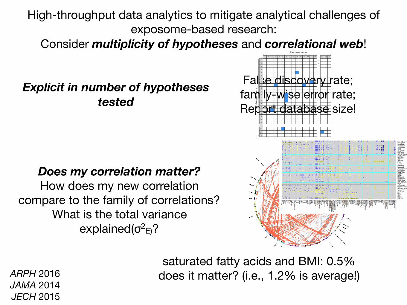
High-throughput data analytics to mitigate analytical challenges of exposome-based research:
Consider multiplicity of hypotheses and correlational web!
Does my correlation matter? How does my new correlation
compare to the family of correlations?What is the total variance
explained(σ2E)?
saturated fatty acids and BMI: 0.5%does it matter? (i.e., 1.2% is average!)
ρ
ARPH 2016 JAMA 2014 JECH 2015
Explicit in number of hypotheses tested
False discovery rate; family-wise error rate;Report database size!
p-2
20
8
1
6
18
7
10
…
p-1
12
2
5
9
4
16
21
11
13
3
17
14
19
p
15
6 101 1482 7 …1311 12 e54 153 9 e-1e-2
…
…
…
…
E exposure factors
P ph
enot
ypic
fact
ors
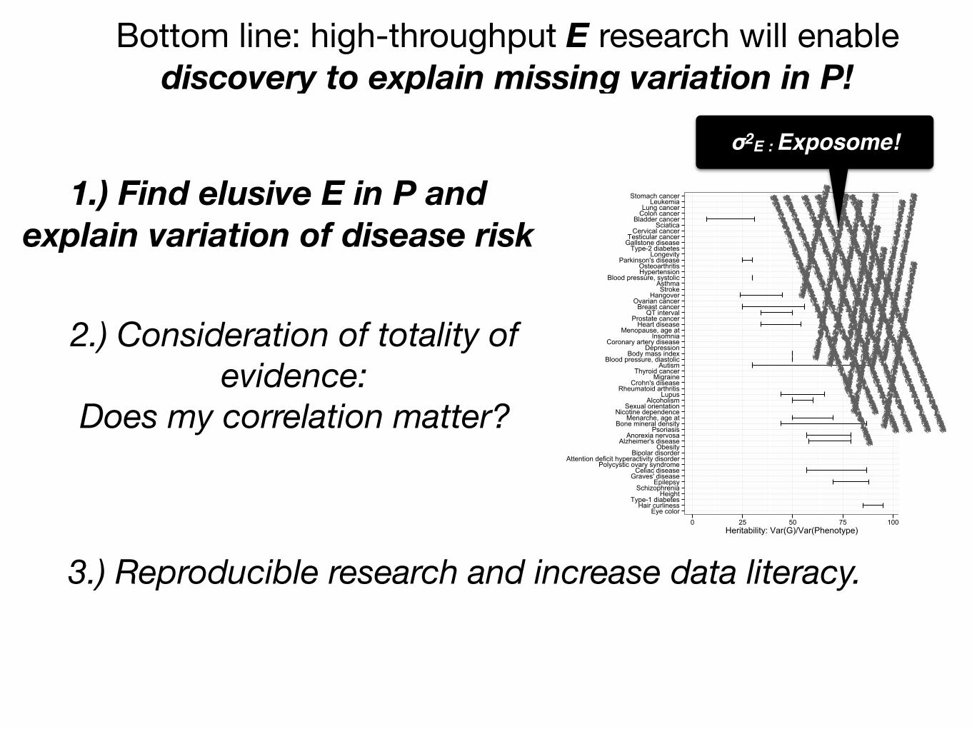
Bottom line: high-throughput E research will enable discovery to explain missing variation in P!
1.) Find elusive E in P and explain variation of disease risk
2.) Consideration of totality of evidence:
Does my correlation matter?
3.) Reproducible research and increase data literacy.
Eye colorHair curliness
Type-1 diabetesHeight
SchizophreniaEpilepsy
Graves' diseaseCeliac disease
Polycystic ovary syndromeAttention deficit hyperactivity disorder
Bipolar disorderObesity
Alzheimer's diseaseAnorexia nervosa
PsoriasisBone mineral density
Menarche, age atNicotine dependence
Sexual orientationAlcoholism
LupusRheumatoid arthritis
Crohn's diseaseMigraine
Thyroid cancerAutism
Blood pressure, diastolicBody mass index
DepressionCoronary artery disease
InsomniaMenopause, age at
Heart diseaseProstate cancer
QT intervalBreast cancer
Ovarian cancerHangoverStrokeAsthma
Blood pressure, systolicHypertensionOsteoarthritis
Parkinson's diseaseLongevity
Type-2 diabetesGallstone diseaseTesticular cancer
Cervical cancerSciatica
Bladder cancerColon cancerLung cancerLeukemia
Stomach cancer
0 25 50 75 100Heritability: Var(G)/Var(Phenotype)
σ2E : Exposome!
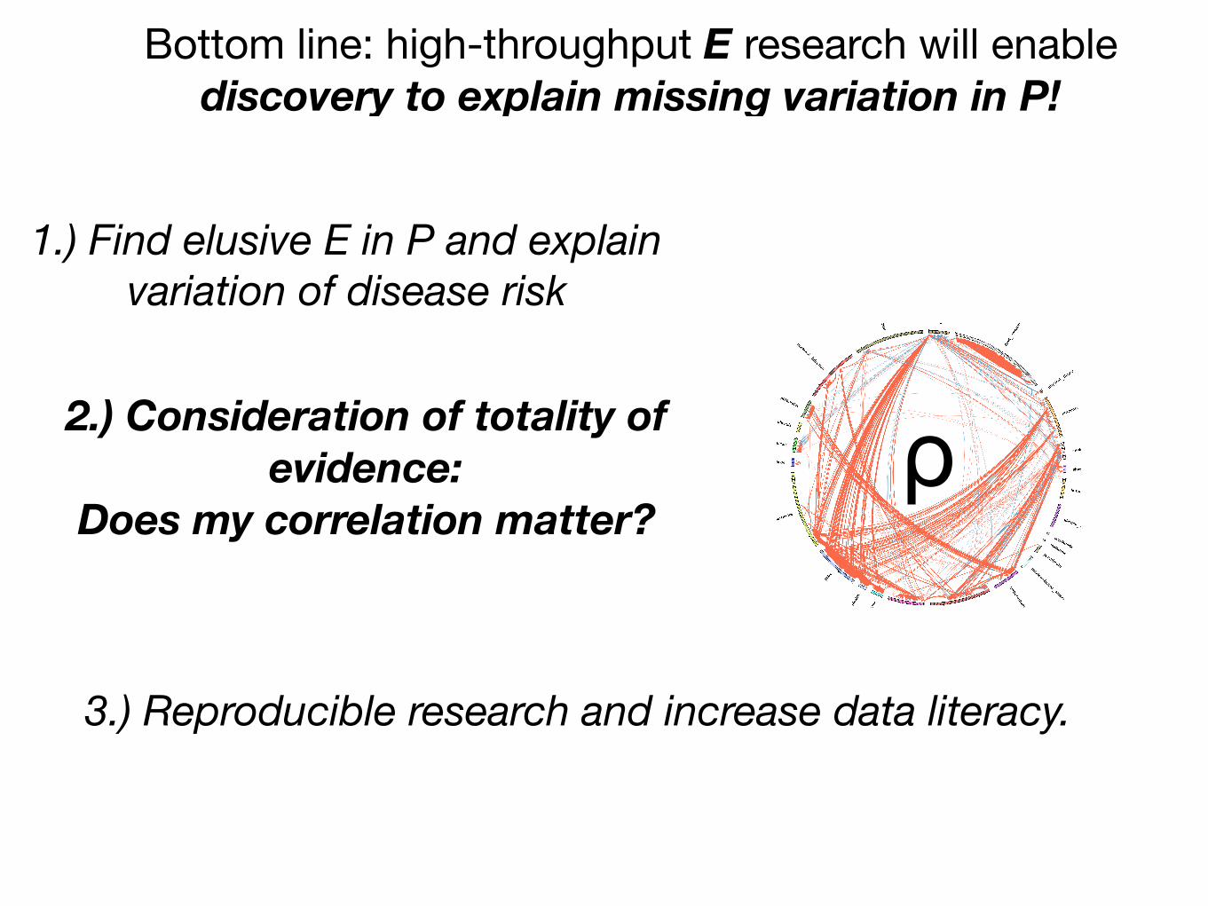
Bottom line: high-throughput E research will enable discovery to explain missing variation in P!
1.) Find elusive E in P and explain variation of disease risk
2.) Consideration of totality of evidence:
Does my correlation matter?
3.) Reproducible research and increase data literacy.
ρ
Bottom line: high-throughput E research will enable discovery to explain missing variation in P!
1.) Find elusive E in P and explain variation of disease risk
2.) Consideration of totality of evidence:
Does my correlation matter?
3.) Reproducible research and increase data literacy.

http://chiragjpgroup.org/exposome-analytics-course
Nam PhoPlease contact me for help or project ideas!

Designing a new children’s study:(1) Increase sample sizes and make data publicly available
(2) Measure G to discover role of E in P
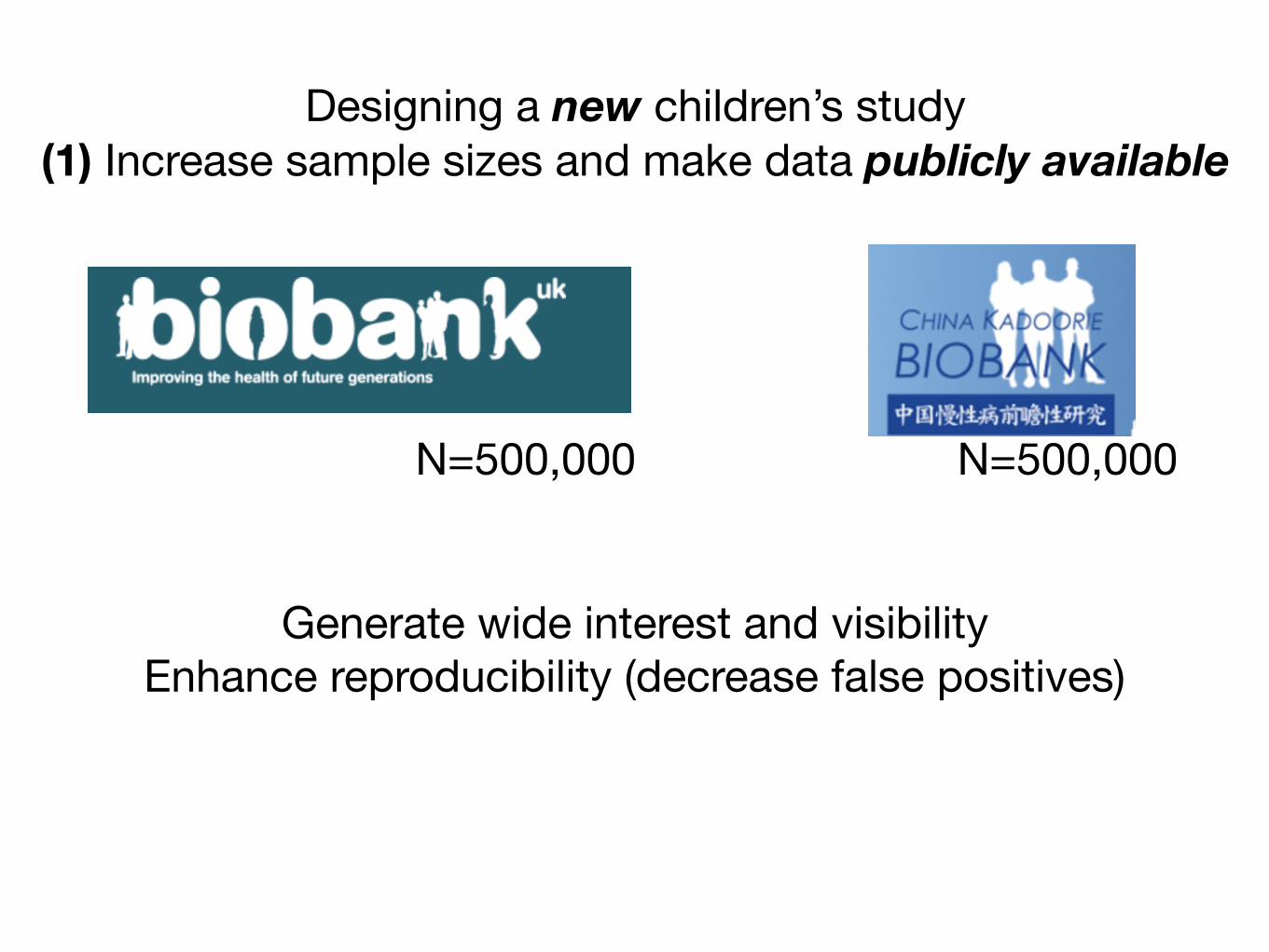
Designing a new children’s study(1) Increase sample sizes and make data publicly available
N=500,000 N=500,000
Generate wide interest and visibilityEnhance reproducibility (decrease false positives)
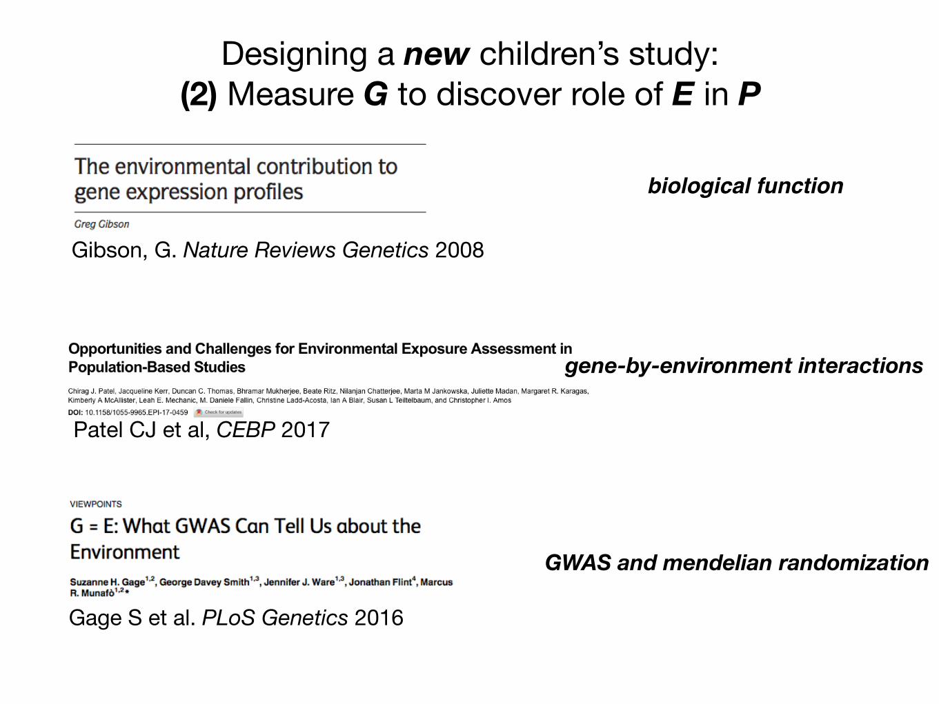
Designing a new children’s study:(2) Measure G to discover role of E in P
Patel CJ et al, CEBP 2017
Gibson, G. Nature Reviews Genetics 2008
biological function
Gage S et al. PLoS Genetics 2016
GWAS and mendelian randomization
gene-by-environment interactions
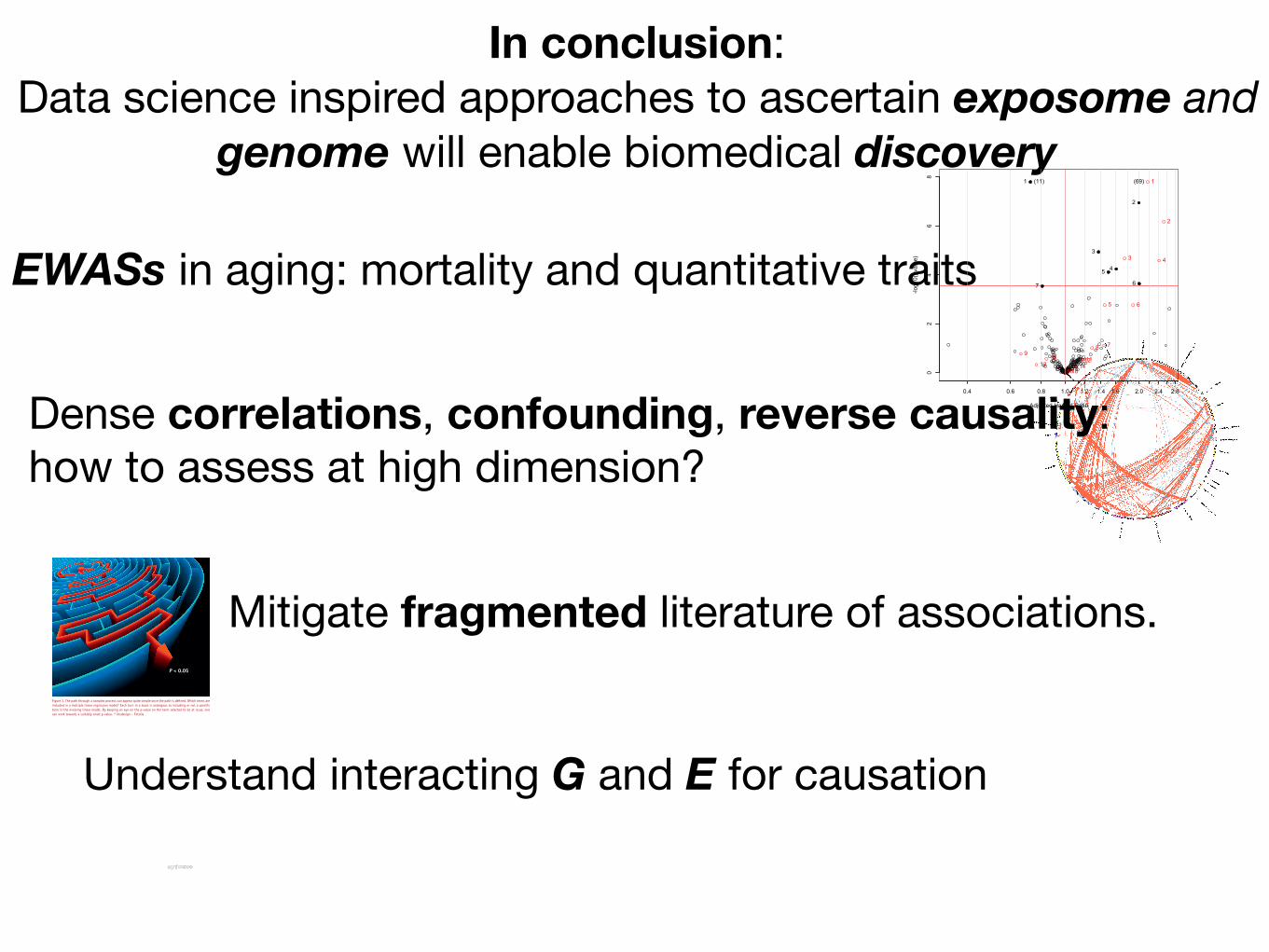
In conclusion:Data science inspired approaches to ascertain exposome and
genome will enable biomedical discovery
Dense correlations, confounding, reverse causality: how to assess at high dimension?
Understand interacting G and E for causation
Mitigate fragmented literature of associations.
september2011 119
Multiple modelling
This problem is akin to – but less well recognised and more poorly understood than – multiple testing. For example, consider the use of linear regression to adjust the risk levels of two treatments to the same background level of risk. There can be many covariates, and each set of covariates can be in or out of the model. With ten covariates, there are over 1000 possible models. Consider a maze as a metaphor for modelling (Figure 3). The red line traces the correct path out of the maze. The path through the maze looks simple, once it is known. Returning to a linear regression model, terms can be put into and taken out of a regression model. Once you get a p-value smaller than 0.05, the model can be frozen and the model selection justified after the fact. It is easy to justify each turn.
The combination of multiple testing and multiple modelling can lead to a very large search space, as the example of bisphenol A in Box 3 shows. Such large search spaces can give small, false positive p-values somewhere within them. Unfortunately, authors and consumers are often like a deer caught in the headlights and take a small p-value as indicating a real effect.
How can it be fixed? A new, combined strategy
It should be clear by now that more than small-scale remedies are needed. The entire system of observational studies and the claims that are made from them is no longer functional, nor is it fit for purpose. What can be done to fix this broken system? There are no principled
ways in the literature for dealing with model selection, so we propose a new, composite strategy. Following Deming, it is based not upon the workers – the researchers – but on the production system managers – the funding agencies and the editors of the journals where the claims are reported.
We propose a multi-step strategy to help bring observational studies under control (see Table 2). The main technical idea is to split the data into two data sets, a modelling data set and a holdout data set. The main operational idea is to require the journal to accept or reject the paper based on an analysis of the modelling data set without knowing the results of applying the methods used for the modelling set on the holdout set and to publish an addendum to the paper giving the results of the analysis of the holdout set. We now cover the steps, one by one.
1 The data collection and clean-up should be done by a group separate from the analysis group. There can be a tempta-tion on the part of the analyst to do some exploratory data analysis during the data clean up. Exploratory analysis could lead to model selection bias.
Box 2. Publication bias
There is general recognition that a paper has a much better chance of acceptance if something new is found. This means that, for publication, the claim in the paper has to be based on a p-value less than 0.05. From Deming’s point of view5, this is quality by inspection. The journals are placing heavy reliance on a statistical test rather than examination of the methods and steps that lead to a conclusion. As to having a p-value less than 0.05, some might be tempted to game the system10 through multiple testing, multiple modelling or unfair treatment of bias, or some combination of the three that leads to a small p-value. Researchers can be quite creative in devising a plausible story to fit the statistical finding.
2 The data cleaning team creates a modelling data set and a holdout set and gives the modelling data set, less the item to be predicted, to the analyst for examination.
P < 0.05
Figure 3. The path through a complex process can appear quite simple once the path is defined. Which terms are included in a multiple linear regression model? Each turn in a maze is analogous to including or not a specific term in the evolving linear model. By keeping an eye on the p-value on the term selected to be at issue, one can work towards a suitably small p-value. © ktsdesign – Fotolia
Table 2. Steps 0–7 can be used to help bring the observational study process into control. Currently researchers analysing observational data sets are under no effective oversight
Step Process / Action
0 Data are made publicly available
1 Data cleaning and analysis separate
2 Split sample: A, modelling; and B, holdout (testing)
3 Analysis plan is written, based on modelling data only
4 Written protocol, based on viewing predictor variables of A
5 Analysis of A only data set
6 Journal accepts paper based on A only
7 Analysis of B data set gives Addendum
EWASs in aging: mortality and quantitative traits
Adjusted Hazard Ratio
-log10(pvalue)
0.4 0.6 0.8 1.0 1.2 1.4 1.6 2.0 2.4 2.8
02
46
8
1
2
3
45
67
1 Physical Activity2 Does anyone smoke in home?3 Cadmium4 Cadmium, urine5 Past smoker6 Current smoker7 trans-lycopene
(11) 1
2
3 4
5 6
789
10 111213 141516
1 age (10 year increment)2 SES_13 male4 SES_05 black6 SES_27 SES_38 education_hs9 other_eth10 mexican11 occupation_blue_semi12 education_less_hs13 occupation_never14 occupation_blue_high15 occupation_white_semi16 other_hispanic
(69)
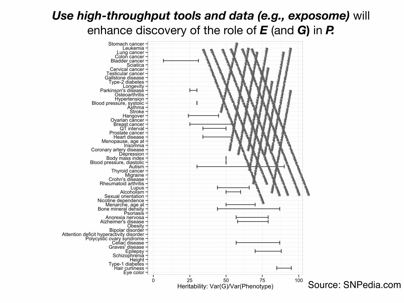
Eye colorHair curliness
Type-1 diabetesHeight
SchizophreniaEpilepsy
Graves' diseaseCeliac disease
Polycystic ovary syndromeAttention deficit hyperactivity disorder
Bipolar disorderObesity
Alzheimer's diseaseAnorexia nervosa
PsoriasisBone mineral density
Menarche, age atNicotine dependence
Sexual orientationAlcoholism
LupusRheumatoid arthritis
Crohn's diseaseMigraine
Thyroid cancerAutism
Blood pressure, diastolicBody mass index
DepressionCoronary artery disease
InsomniaMenopause, age at
Heart diseaseProstate cancer
QT intervalBreast cancer
Ovarian cancerHangoverStrokeAsthma
Blood pressure, systolicHypertensionOsteoarthritis
Parkinson's diseaseLongevity
Type-2 diabetesGallstone diseaseTesticular cancer
Cervical cancerSciatica
Bladder cancerColon cancerLung cancerLeukemia
Stomach cancer
0 25 50 75 100Heritability: Var(G)/Var(Phenotype) Source: SNPedia.com
Use high-throughput tools and data (e.g., exposome) will enhance discovery of the role of E (and G) in P.

raj (ex officio) chirag “the better” adam grace danielle yeran
sivateja jake kajalalan
RagGroup Data Science Team:2 post-docs, 3 PhD, 2 MS, 1 HS, 2 visiting
PhD: systems biology, integrative genomicsMS: statistics (HSPH)
Post-docs: biology, medicine, and mathematics
nam

Harvard DBMI Susanne ChurchillNathan PalmerSophia MamousetteSunny AlvearMichal Preminger
Chirag J [email protected]
@chiragjpwww.chiragjpgroup.org
NIH Common FundBig Data to Knowledge
AcknowledgementsRagGroup Nam Pho Jake Chung Kajal Claypool Arjun Manrai Chirag Lakhani Adam BrownDanielle RasoolyAlan LeGoallecSivateja Tangirala
IEA-WCE 2017 symposium Shoji Nakayama
Junya Kasamatsu Ministry of Environment (Japan)
Mentioned Collaborators Isaac KohaneJohn IoannidisDennis BierHugo Aschard