jason ashley taylor - auburn university
TRANSCRIPT
ONLINE IN-SITU ESTIMATION OF NETWORK PARAMETERS UNDER INTERMITTENT
EXCITATION CONDITIONS
Except where reference is made to the work of others, the work described in this dissertation is my own or was done in collaboration with my advisory committee. This dissertation does not
include proprietary or classified information.
Jason Ashley Taylor
Certificate of Approval:
Charles A. Gross S. Mark Halpin, Chair Professor Professor Electrical and Computer Engineering Electrical and Computer Engineering R. M. Nelms George Flowers Professor Interim Dean Electrical and Computer Engineering Graduate School

ONLINE IN-SITU ESTIMATION OF NETWORK PARAMETERS UNDER INTERMITTENT
EXCITATION CONDITIONS
Jason Ashley Taylor
A Dissertation
Submitted to
the Graduate Faculty of
Auburn University
in Partial Fulfillment of the
Requirements for the
Degree of
Doctor of Philosophy
Auburn, Alabama August 9, 2008

iii
ONLINE IN-SITU ESTIMATION OF NETWORK PARAMETERS UNDER INTERMITTENT
EXCITATION CONDITIONS
Jason Ashley Taylor
Permission is granted to Auburn University to make copies of this dissertation at its discretion, upon request of individuals or institutions at their expense. The author
reserves all publication rights.
Signature of Author
Date of Graduation

iv
VITA
Jason Ashley Taylor, son of Charles and Virginia Taylor, was born November 25,
1975 in Biloxi, Mississippi. He received B.S. and M.S. degrees in Electrical Engineering
from Mississippi State University in 2000 and 2002. He worked as a Power Systems
Engineer at Electrotek Concepts from 2002 to 2004 before pursing a Ph.D. in Electrical
Engineering. While at Auburn University, he worked as an Assistant Instructor, Teaching
Assistant, and Graduate Research Assistant.

v
DISSERTATION ABSTRACT
ONLINE IN-SITU ESTIMATION OF NETWORK PARAMETERS UNDER INTERMITTENT
EXCITATION CONDITIONS
Jason Taylor
Doctor of Philosophy, August 9, 2008 (M.S. Mississippi State University, 2002) (B.S. Mississippi State University, 2000)
176 Typed Pages
Directed by S. Mark Halpin
Online in-situ estimation of network parameters is a potential tool to evaluate
electrical network and conductor health. The integration of the physics-based models
with stochastic models can provide important diagnostic and prognostic information.
Correct diagnoses and prognoses using the model-based techniques therefore depend
on accurate estimations of the physical parameters. As artificial excitation of the
modeled dynamics is not always possible for in-situ applications, the information
necessary to make accurate estimations can be intermittent over time. Continuous
online estimation and tracking of physics-based parameters using recursive least-
squares with directional forgetting is proposed to account for the intermittency in the

vi
excitation. This method makes optimal use of the available information while still
allowing the solution to following time-varying parameter changes. Computationally
efficient statistical inference measures are also provided to gauge the confidence of
each parameter estimate. Additionally, identification requirements of the methods
and multiple network and conductor models are determined. Finally, the method is
shown to be effective in estimating and tracking parameter changes in both the DC
and AC networks as well as both time and frequency domain models.

vii
ACKNOWLEDGEMENTS
I wish to express my appreciation to my advisor, Dr. Mark Halpin, for his shared
experience, guidance, and patience. I would also like to acknowledge the significant
contributions from my committee members, Dr. Mark Nelms and Dr. Charles Gross,
whose instruction and advice proved invaluable throughout my academic endeavors.
Additionally, I thank my family and friends for their support and encouragement in
completing this work. Most importantly, the author wishes to recognize the contributions
of his best friend and wife Robin. Her never ending encouragement and support provided
both foundation and motivation to accomplish such an undertaking. Thank you.

viii
Style manual:
IEEE Editorial Style Manual
The Chicago Manual of Style, University of Chicago Press
Computer software:
Microsoft Word
Microsoft Excel
MATLAB
PSPICE

ix
TABLE OF CONTENTS
LIST OF FIGURES ................................................................................................................ xii
LIST OF TABLES ................................................................................................................. xv
NOMENCLATURE............................................................................................................... xvi
CHAPTER 1 Introduction.................................................................................................. 1
CHAPTER 2 Literature Review ........................................................................................ 6
2.1. Electrical Machine and Transformer Condition Monitoring ................................ 9
2.2. Cable Diagnostic Methods.................................................................................. 12
2.3. Cable Parameter Estimations Methods............................................................... 16
CHAPTER 3 Recursive Parameter Estimation................................................................ 19
3.1. Identifiability ...................................................................................................... 20
3.2. Recursive Least-Squares..................................................................................... 24
3.2.1. Directional Forgetting ................................................................................ 34
3.2.2. Variable Directional Forgetting.................................................................. 37
3.2.3. Covariance Resetting.................................................................................. 39
3.2.4. Multivariable Solutions .............................................................................. 41
3.3. Model and Parameter Validation ........................................................................ 42
3.3.1. Margins of Error ......................................................................................... 43
3.3.2. Multicollinearity Tests ............................................................................... 46
3.3.3. Residual Analysis ....................................................................................... 48
x
3.4. Measurement Noise ............................................................................................ 50
3.4.1. Quantization and Sampling Rate................................................................ 51
3.4.2. Filtering ...................................................................................................... 52
3.5. Normalization ..................................................................................................... 53
CHAPTER 4 Two-Condcutor Models............................................................................. 55
4.1. Short Transmission Line Model ......................................................................... 58
4.2. Nominal Pi Circuit Model .................................................................................. 61
4.2.1. SISO Model ................................................................................................ 64
4.2.2. MISO Model............................................................................................... 66
4.2.3. SISO/MISO Model..................................................................................... 68
4.2.4. Shunt Conductance..................................................................................... 69
4.3. Model Evaluations .............................................................................................. 70
4.4. Summary............................................................................................................. 92
CHAPTER 5 Multiple Conductor Models....................................................................... 93
5.1. Identifiability .................................................................................................... 101
5.2. Model Evaluations ............................................................................................ 106
5.2.1. Series Element Model .............................................................................. 110
5.2.2. Shunt Element Model ............................................................................... 121
5.2.3. Full Parameter Model ............................................................................... 122
5.3. Summary........................................................................................................... 126
CHAPTER 6 Frequency-Domain Models ...................................................................... 128
6.1. Line Models ...................................................................................................... 128
6.2. Thevenin Equivalent......................................................................................... 130
6.2.1. Time-Domain ........................................................................................... 131
6.2.2. Frequency-Domain................................................................................... 133
6.3. Parameter Estimate Accuracy........................................................................... 136
6.4. Model Evaluations ............................................................................................ 138
6.5. Summary........................................................................................................... 145

xi
CHAPTER 7 Conclusions.............................................................................................. 146
7.1. Summary........................................................................................................... 146
7.2. Future Work...................................................................................................... 148
Bibliography ................................................................................................................... 150
xii
LIST OF FIGURES
Figure 1-1. Continuous Online Diagnostic and Prognostic Monitor .................................. 4
Figure 2-1. Model Reference Approach ............................................................................. 7
Figure 2-2. Prognosis Technical Approaches [5] ............................................................... 8
Figure 3-1. Condition Monitor Parameter Estimation and Validation Block................... 43
Figure 4-1. Distributed Parameter Line ............................................................................ 56
Figure 4-2. Short Transmission Line Circuit Model......................................................... 58
Figure 4-3. Two-Conductor Mutually Coupled Circuit.................................................... 62
Figure 4-4. Nominal Pi Equivalent Circuit ....................................................................... 64
Figure 4-5. Single-Phase Test Circuit.............................................................................. 71
Figure 4-6. Test Case Voltages and Currents ................................................................... 73
Figure 4-8. SISO/MISO Model Parameter Estimates during a Load Change. ................. 74
Figure 4-9. Parameter Estimates with 32-Bit Quantization Error..................................... 75
Figure 4-10. Parameter Estimates with 16-Bit Quantization Error and λc = 0.999. ......... 76
Figure 4-11. Parameter Estimates for Step Change in R. ................................................. 77
Figure 4-12. Parameter Estimates for Step Change in C. ................................................. 77
Figure 4-13. MIMO Model Parameter Estimates ............................................................ 79
Figure 4-14. 95% Confidence Margins of Error.............................................................. 79
Figure 4-15. MISO Model Parameter Estimates using RLS/DF ..................................... 80
xiii
Figure 4-16. 95% Confidence Margins of Error.............................................................. 81
Figure 4-17. Prediction Error Autocorrelation.................................................................. 81
Figure 4-18. Sending End Voltage and Current Waveforms........................................... 82
Figure 4-19. Parameter Estimates using RLS................................................................... 83
Figure 4-20. Parameter Estimates using RLS/DF............................................................. 83
Figure 4-21. Parameter Estimates using RLS/DF............................................................ 84
Figure 4-22. Parameter Estimates using RLS.................................................................. 85
Figure 4-23. Parameter Estimates using RLS/VDF......................................................... 86
Figure 4-24. DC Signals for a Switching DC Load......................................................... 89
Figure 4-25. Parameter Estimates using RLS/DF............................................................ 91
Figure 4-26. Parameter Estimates using RLS................................................................... 91
Figure 5-1. Multiple Conductor Line Model .................................................................... 94
Figure 5-2. Four-Conuctor Line Model ............................................................................ 99
Figure 5-3. Single Line Diagram of the Three-Phase Test System ................................ 108
Figure 5-4. Test System Voltage and Current Waveforms............................................. 111
Figure 5-5. Multi-conductor Parameter Estimates.......................................................... 113
Figure 5-6. 95% Confidence Margins of Error............................................................... 113
Figure 5-7. A-Phase Correlation Matrices ...................................................................... 114
Figure 5-8. Multi-conductor Parameter Estimates.......................................................... 115
Figure 5-9. B-Phase Correlation Matrix ......................................................................... 116
Figure 5-10. Multi-conductor Parameter Estimates........................................................ 117
Figure 5-11. 95% Confidence Margins of Error............................................................. 117
Figure 5-12. Parameter Estimates using RLS/DF........................................................... 118
xiv
Figure 5-13. Correlation Matrix for A-phase Estimations.............................................. 119
Figure 5-14. 95% Margins of Error ................................................................................ 119
Figure 5-15. Parameter Estimates using RLS................................................................. 120
Figure 5-16. Parameter Estimates using RLS (Upper) and 95% Confidence Margins
of Error (Lower)............................................................................................. 122
Figure 5-17. Parameter Estimates using RLS/DF........................................................... 124
Figure 5-18. 95% Confidence Margins of Error............................................................. 125
Figure 5-19. Parameter Estimates using RLS/DF........................................................... 126
Figure 6-1. Thevenin Equivalent Circuit for hth Order Harmonic Frequency ................ 134
Figure 6-2. Frequency-Domain Thevenin Equivalent Estimation Method .................... 136
Figure 6-3. Single-Phase Test Network .......................................................................... 139
Figure 6-4. Network Transfer Impedances Seen at Bus 3 .............................................. 140
Figure 6-5. Input-Output Phasor Components at 60 Hz ................................................. 141
Figure 6-6. 60 Hz Thevenin Equivalent Parameter Estimates........................................ 143
Figure 6-7. Covariance Matrix Diagonals ...................................................................... 143
Figure 6-8. Input-Output Phasor Components at 300 Hz ............................................... 144
Figure 6-9. 300 Hz Thevenin Equivalent Parameter Estimates...................................... 145
xv
LIST OF TABLES
Table 3-1. Recursive Least-Squares Methods .................................................................. 40
Table 3-2. Time Domain Per-Unit Base Relationships .................................................... 54
Table 4-1. Test System Per-Unit Bases ............................................................................ 72
Table 4-2. 95% Univariate Confidence Intervals ............................................................. 88
Table 5-1. Four-Conductor Example Parameters ........................................................... 107
Table 5-2. Test System Per-Unit Bases .......................................................................... 108
Table 5-3. Voltage Fourier Components for Balanced Conditions ................................ 111
Table 5-4. Current Fourier Components for Balanced Conditions................................. 111
Table 5-5. Voltage Fourier Components for Unbalanced Conditions ............................ 112
Table 5-6. Current Fourier Components for Unbalanced Conditions............................. 112
Table 6-1. Thevenin Equivalent Circuit Data ................................................................. 140
Table 6-2. Test System Events........................................................................................ 141

xvi
NOMENCLATURE
Vector-Matrix Notation
a: Scalar
A: Matrix
a~ : Vector
a : Complex Scalar
A : Matrix of complex values
a~ : Vector of complex values
AR: Real component of a complex number
AI: Imaginary component of a complex number
Solution Variables
cov(θ ): Matrix of parameter estimate covariances
C: Correlation matrix
e: Residual error
I: Identity matrix
J(θ ): Sum of the squared residuals
k: Discrete time index

xvii
L~ : Parameter update gain vector
n: Number of measurements over time
p: Number of unknown parameters
P: Covariance matrix
Pjj: Jth diagonal of the covariance matrix
q: Quantization step size
R: Information matrix
Rjj: Jth diagonal of the information matrix
SIF: Standard deviation influence factor
T0: Exponential delay time constant
VIF: Variance inflation factor
ε : Prediction error
θ~ : Unknown parameter vector
λ: Exponential forgetting factor
ρ : Differential operator dtd
ϕ~ : Regressor vector
Φ : Regressor matrix
σ 2: Residual error variance
Model Variables
C: Capacitance
G: Shunt conductance

xviii
i: Instantaneous current
I : Frequency-domain phasor current
L: Inductance
R: Resistance
s: Laplacian operator
t: Instantaneous time
T: Sampling period
u: Input regressor
v: Instantaneous voltage
V : Frequency-domain phasor voltage
y: Dependent variable / Output variable
Abbreviations and Acronyms
CI: Confidence Interval
DF: Directional forgetting
FFT: Fast Fourier transform
MIMO: Multiple-input multiple-output models
MISO: Multiple-input single-output models
PE: Persistence of excitation
RLS: Recursive least-squares
RLS/DF: Recursive least-squares with directional forgetting
RLS/VDF: Recursive least-squares with variable directional forgetting

xix
SISO: Single-input single-output models
TF: Transfer function method

1
CHAPTER 1
INTRODUCTION
Recent trends in large vehicular design indicate an increased reliance on electrical
networks for power delivery. Whether the vehicle is a naval ship, space shuttle, or space
station, networks are typically characterized by low to medium voltages and known
system configurations. Poor performance, undesired operation, or faults in these networks
can severely degrade or even damage the system. In many networks, little indication of a
potentially harmful disturbance or failure is given until an event actually occurs.
Furthermore, disturbances such as weak connections, temporary faults, and changing
environmental conditions are difficult to diagnose using offline tests. As a result,
continuous in-situ monitoring of the network provides better information from which to
evaluate the network’s health.
Assuming continuous in-situ monitoring (evaluation in the normal operating
environment), online diagnostic evaluation can be achieved through direct analysis of
measured waveforms and through estimation of characteristic parameters. In the first
approach, measured voltage and current waveforms are compared to known “good”
waveforms or metrics to evaluate network conditions such as open and short-circuits. In
the second approach, parameters characterizing the network’s physical properties can be
2
estimated from measured “input-output” data. By defining model structures in terms of
known physical relationships, also known as “gray box” models, the estimated
parameters can be compared to known acceptable ranges. As the monitoring is
continuous, trending of estimates can distinguish normal changes from problematic
conditions. Therefore, parameter identification and tracking provides an approach from
which to evaluate both diagnostic and prognostic health.
Many online and offline diagnostic methods apply known external stimuli in order to
excite particular dynamic responses [1]. These stimuli are typically tailored to a particular
application and require some physical means by which to induce or inject the signals.
However, controlling the input stimuli artificially is an unappealing option for a vehicle
electrical network. The required stimulus is either too harmful for online applications, as
with over-voltage tests, or too specific to be easily implemented for a wide variety of
equipment and network configurations. Furthermore, the extra space and weight required
to generate and inject the stimuli is prohibitive in mobile applications. For these reasons,
passive monitoring of the network will be evaluated. The term passive is used here to
indicate that no control or influence is exerted over the system inputs.
Still, without actively controlling the input stimuli there is no guarantee that the
measured waveforms contain sufficiently “rich” information to base the parameter
estimates. As richness of the information depends upon the system’s normal and
abnormal operation, sufficient excitation of the modeled dynamics will potentially vary
over time. Under the assumption of passive monitoring, accurate estimation of the

3
characteristic network parameters requires a method that efficiently utilizes intermittently
available information.
The goal of this research is to identify and develop parameter estimation techniques
which are suitable to the estimation of network parameters given passive monitoring of
network elements in their operating environment. Once the approximations of the
characteristic parameters are available, statistical analysis of these values over time
provides diagnostic and prognostic measures of network health. The parameter estimates
are therefore the foundation of the network health monitoring device illustrated in Figure
1-1. Accuracy of the parameter estimates will obviously have a profound influence over
the performance of the diagnostic and prognostic measures. Recursive least-squares
techniques are selected to fit the parameter estimates to the measured data as these
algorithms are numerically efficient and provide fast accurate estimates. Given their
importance to the condition monitoring method, the criteria and conditions under which
the algorithms provide accurate estimations are examined in detail in Chapter 3.
Additionally, statistical inference measures are provided to gauge the level of confidence
in the estimates.
In order to be effective, the method represented in Figure 1-1 requires monitoring the
network conditions over extended periods to ensure sufficient information concerning the
dynamics is observed. Intuitively, the more information a data set contains about a
modeled dynamic, the better the parameter estimate and consequently the diagnostic and
prognostic measures. While system disturbances impact the estimates by increasing the
dynamic content, the system is not intended as a fast acting protection device. In other

4
words, the monitoring system’s purpose is to observe the slow time varying parameter
changes in an attempt to predict future disturbances. Additionally, the observations
provide for prognostic evaluation via resulting parameter estimates as well as
examination of the measurements themselves. However, the parameter identification
procedures are not intended to be quick enough to provide fast acting protection from
faults and other disturbances.
Source System/Load
Measured Waveforms
Voltages
Currents
Parameter Estimation & Identification Algorithm
Monitored Device
Model-Based Diagnosis and Prognosis
Historical Measurement Data &
Signature Analysis
Data Reporting and Monitor Control
Filtering and A/D Conversion
System Monitoring Device
Figure 1-1. Continuous Online Diagnostic and Prognostic Monitor

5
As indicated in Figure 1-1, the estimations are reliant upon measurement type and
location, accurate measurement and quantization, in addition to the parameter
identification algorithm. However, another key factor is the model selected to represent
the monitored element’s physical characteristics. It is assumed that the physical
characteristics of the monitored network elements (single conductor and multiple
conductor cables, etc.) are describable by linear differential equations. The identifiability
requirements of potential two-conductor line models are examined in Chapter 4 along
with the ability of the identification algorithms. These findings are then extrapolated
further to branches with multiple conductors in Chapter 5. Additionally, the identifiability
requirements of the network connected elements using frequency-domain measurement
are examined in Chapter 6. While the derived models mostly consider wiring or cables,
other networked equipment can be approached in the same manner as long as an accurate
linear model can be specified. The parameter estimation algorithms and statistical
inference measures were implemented in MATLAB and validated using test data
generated in PSPICE.

6
CHAPTER 2
LITERATURE REVIEW
Condition monitoring is the use of advanced technologies in order to determine
equipment condition and potentially predict failure. Methods of conditioning monitoring
have been researched and successfully implemented in areas such as industrial
applications and transportation. Regardless of the application, these methods share a
common goal of detection and diagnosis of unacceptable changes in system parameters,
also known as process faults. Accurate assessment of the monitored device’s health is
therefore dependent on the ability to correctly detect and interpret characteristic
parameters changes.
In general, fault detection and diagnosis approaches are divided into two categories:
direct analysis methods and model-based methods. Direct analysis methods apply
techniques such as logic reasoning, reflectometry, and signature analysis directly to the
monitored or observed values. In contrast, model-based methods use the observations in
combination with mathematical models to generate quantitative values which can also be
analytically evaluated [2]. As Simani et al. stated in [3], “If a fault occurs, the residual
signal (i.e. the difference between the real system and model behavior) can be used to
diagnose and isolate the malfunction.” The generation of the residual signal using a
7
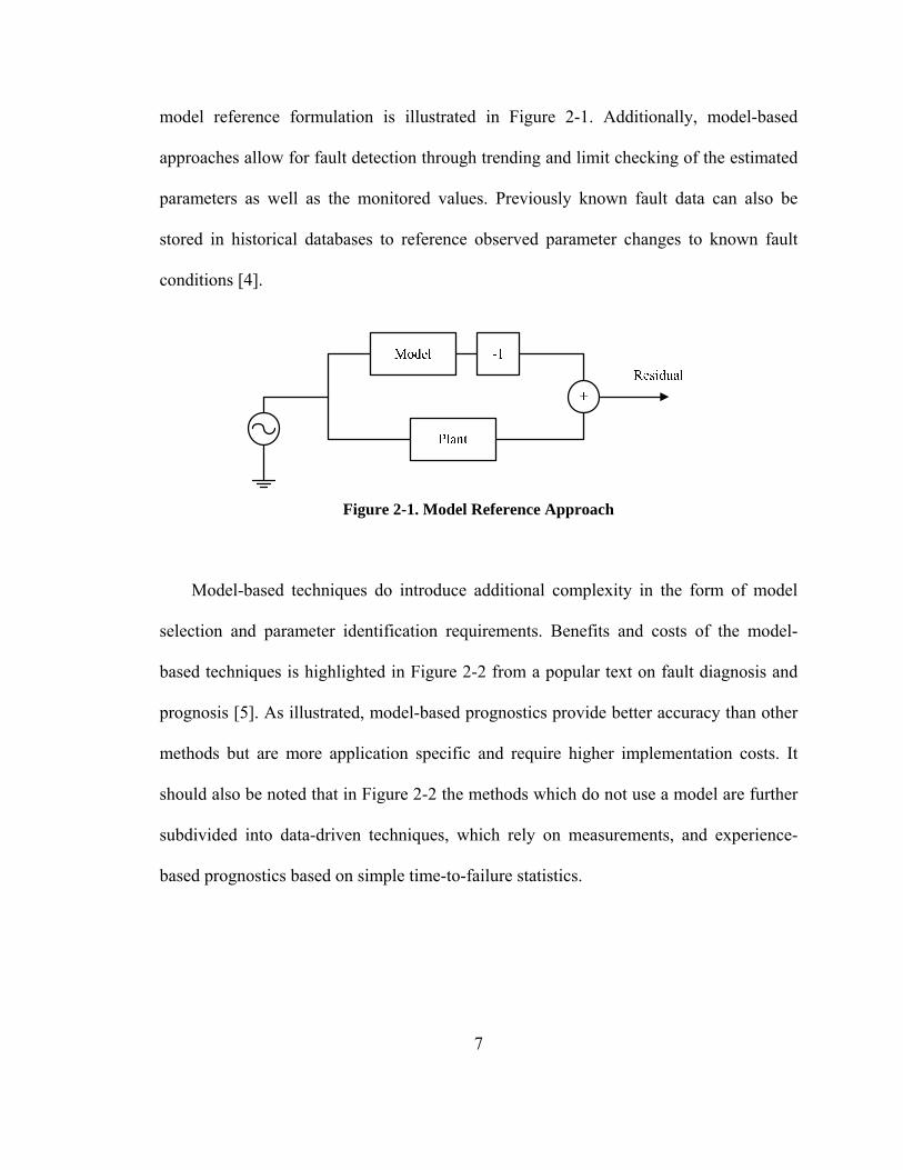
model reference formulation is illustrated in Figure 2-1. Additionally, model-based
approaches allow for fault detection through trending and limit checking of the estimated
parameters as well as the monitored values. Previously known fault data can also be
stored in historical databases to reference observed parameter changes to known fault
conditions [4].
Figure 2-1. Model Reference Approach
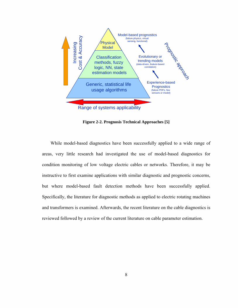
Model-based techniques do introduce additional complexity in the form of model
selection and parameter identification requirements. Benefits and costs of the model-
based techniques is highlighted in Figure 2-2 from a popular text on fault diagnosis and
prognosis [5]. As illustrated, model-based prognostics provide better accuracy than other
methods but are more application specific and require higher implementation costs. It
should also be noted that in Figure 2-2 the methods which do not use a model are further
subdivided into data-driven techniques, which rely on measurements, and experience-
based prognostics based on simple time-to-failure statistics.
8
Range of systems applicability
Incr
easi
ngC
ost &
Acc
urac
y
Classification methods, fuzzy logic, NN, state
estimation models
PhysicalModel
Generic, statistical life usage algorithms
Experience-basedPrognostics(failure PDFs, few sensors or model)
Evolutionary or trending models
(data-driven, feature-based correlation)
Model-based prognostics(failure physics, virtual
sensing, functional) Prognostic approach
Figure 2-2. Prognosis Technical Approaches [5]
While model-based diagnostics have been successfully applied to a wide range of
areas, very little research had investigated the use of model-based diagnostics for
condition monitoring of low voltage electric cables or networks. Therefore, it may be
instructive to first examine applications with similar diagnostic and prognostic concerns,
but where model-based fault detection methods have been successfully applied.
Specifically, the literature for diagnostic methods as applied to electric rotating machines
and transformers is examined. Afterwards, the recent literature on the cable diagnostics is
reviewed followed by a review of the current literature on cable parameter estimation.
9
2.1. ELECTRICAL MACHINE AND TRANSFORMER CONDITION MONITORING
A large body of research has focused on condition monitoring of rotating electric
machines due to the high mechanical and electrical stress involved and the potential for
catastrophic failure. Given their importance in industry, much of the literature has been
directed towards induction motors. A comprehensive bibliography of induction motor
condition monitoring methods was given in [6] and a good overview of fault detection in
induction motors using signature analysis was provided in [7]. Background of
implemented model-based methods can be found in [8, 9]. Additionally, a comparison
between signature analysis methods and model-based methods for induction motor fault
diagnostics was recently examined by Harihara et al. in [10]. For the given methods and
selected models, Harihara et al. were able to show that the probability of false alarms was
reduced by 40% when using the model-based solution. Furthermore, in a study performed
by Nasiri et al. [11], tracking of modeled parameter estimates was shown to be a useful
indicator of rotor fault conditions.
Model-based condition monitoring has been proposed for other machine types as
well, for example [7, 12, 13]. In [12], a method was introduced for the offline diagnostic
testing of electromechanical actuators to replace current hydraulic/pneumatic actuators in
aircraft. The method represented the actuator’s brushless DC motor using a set of
physically based discrete time transfer functions. Through perturbations introduced into
the control signal, system identification techniques were used to estimate the physical
parameters from the observed voltage, current, and rotor speed changes. Test bed
evaluations demonstrated the method to be capable of accurately estimating key physical

10
parameters including resistance, inductance, and rotor inertia. A supervisory system using
fuzzy logic was then shown to be successful at diagnosing potential faults from the
estimated parameter changes.
In recent decades, significant research into electrical-based diagnostics of power
transformers has also been conducted. A technique which received a great deal of
attention is the transfer function (TF) method which derived multiple transfer function
models from input-output measurements. Malewski and Poulin first proposed the use of
transfer functions in 1988 to account for difficulties in obtaining comparable historic
voltage and current waveform data [14]. As transfer functions are independent of the
applied impulse, the historical transfer functions could be generated without requiring the
a consistent input stimuli. Mechanical deformations in the winding arising from short-
circuits and mechanical stresses during installation could then be detected by comparing
measured TF models to accepted reference models [15].
Initially transfer functions were generated through the application of broadband
pulses and time-domain measurements. The transfer functions were then determined as
the ratio of the Fourier transformed input-output measurements. A second method
determined the transfer function directly in the frequency domain by using a variable
frequency sinusoid. At each frequency, phasor input and output measurements describe
the transfer function at that particular frequency. Hence, the transfer function was
measured by sweeping the frequency of the sinusoidal input across the desired bandwidth
and recording the quotient between the phasor input and output at each frequency. The
frequency-domain approach has gained prominence in offline tests because it eliminates

11
signal-to-noise ratio, frequency resolution, and aliasing issues associated with the time-
domain approach [15]. However, the time-domain approach was often utilized as the
default method for online applications where the input stimuli could not be controlled.
Leibfried and Feser examined both online and offline tests for in service power
transformers in [16]. On-site “offline” test inputs were applied by switching the high
voltage side of the transformer in and out of service to create impulses. In contrast,
“online” tests used transients induced by some external network event. Some of the
difficulties expressed by Leibfried and Feser for the on-site tests were the requirements of
identical tap-changer settings and similar temperatures in order to produce comparable
transfer functions. In addition, reflected traveling waves from the interconnected network
could potentially bias the transfer function estimation. In principle, reflected waveforms
observed in input will not change the model estimate; however, reflections in the
observed outputs may be misinterpreted as changes in the transformer. Wimmer and
Feser revisited this issue and proposed limiting the calculation of the transfer function
from single waveform peaks [17].
The simplest use of the TF method is a pass-fail test. If the measured transfer
function is in agreement with the reference model, typically generated directly after it is
manufactured, then no defect can be detected. However, if the measured TF deviates
substantially from the reference, the transformer is deemed faulty and removed from
service. This simple comparison, however, does not provide any information about what
specific defect may have occurred. This limitation was pointed out by Leibfried and Feser
who noted at the time that, “there is no reliable information about the relationship

12
between changes – mechanical or dielectric – of the winding assembly and their effect on
the transfer function” [16].
Transfer functions are black-box models or models which do not contain a-priori
knowledge of the underlying physical relationships. Recent endeavors have concentrated
on correlating physical relationships with the transfer function in an effort to provide
detailed fault diagnostics. A sensitivity test of the transfer function was performed by
Mikkelson et al. in [18] which showed that physical changes in the oil, core, and winding
insulation influenced the overall shape of the transfer function. A similar study was
performed by Rahimpour et al. [19] that showed correlation between transfer function
changes and a model of physical displacement in the transformer windings. In
Rahimpour’s model, the parameters were determined analytically based on known
physical relationships not through monitored conditions and parameter estimation
techniques. While research in this area is ongoing, the lack of technical articles using
parameter estimation techniques to determine physics-based parameters is demonstrative
of the difficulties involved with proper model selection and subsequent estimation of
characteristic parameters.
2.2. CABLE DIAGNOSTIC METHODS
One of the simplest electrical cable tests is to measure the resistance of the cable. If
the measured resistance is too high it is an indication that the wire is not connected or
open circuited. Measurement of the capacitance or inductance can also be used to
determine the length of the wire by comparing the cable’s known distributed capacitance

13
and inductance with the calculated values. As the lumped capacitance and inductance
increase with the length of the wire, smaller than expected values can be used to
approximate location of the open or short circuit fault. However, errors can occur in these
fault locations estimation whenever the distributed parameter values are not constant over
the length of the wire. Additionally, these tests cannot be performed while the wire is in
use.
In electrical networks, identification and protection of large abrupt faults is generally
well understood. Slowly occurring or incipient faults are more difficult to detect and
diagnose given the many factors involved. Experiences with incipient faults in cable
splices led to the development of the fault specific relay detector described in [20]. The
incipient faults resulted from accumulation of water in cable splices which eventually
lead to an arcing event. The arc caused the water to evaporate but the resulting
combination of pressure and moisture also cleared the fault. The whole process of arcing
and self-clearing occurred within less that a quarter-cycle (4.16ms) which was
insufficient to cause the overcurrent protection to operate. Due to the continued
degradation of the splice, the frequency of these events tends to increase over time. The
developed relay operation depends on a known relationship between the disturbance and
its symptoms. In particular, the disturbance is characterized by flashovers at the voltage
peaks, quarter-cycle overcurrents, and an increasing frequency of occurrence. Once these
characteristics are observed, the relay acts by operating protection equipment or signaling
an operator. Detection of other types of incipient faults in this manner would require
similar a-priori knowledge. While most research utilizing signature analysis techniques

14
tends to concentrate on the diagnostic of medium and high voltage cables, reflectometry
techniques have recently been investigated for the detection and location of faults in
aircraft wiring [21-25]. However, these methods do not use model-based techniques and
currently can only detect existing faulted conditions.
A few recent studies have focused on incipient fault location in distribution networks
in the United Kingdom. In [26] the transient voltage and current waveforms are recorded
by a digital disturbance recorder. Assuming known cable impedance characteristics, the
fault location was either extrapolated from measurements at multiple locations or through
measured transient impedances. Experiences and common causes of incipient faults in
underground low voltage networks were also explored by Walton in [27]. While Walton
indicated that waveform analysis was used successfully to identify incipient fault
locations, he also pointed out the need for online condition assessment.
Another application where cable condition assessment has received strong interest is
within nuclear power plants. Exposure of cables to harsh environmental conditions in
these plants raised interest in condition monitoring of low voltage cable insulation.
Concerns over how to assess the aging and degradation of insulation have led to the
requirement of long-term studies of cable materials in nuclear power plants by
IEEE/ANSI Standard 383 [28]. Additionally, a detailed summary of aging factors and
tests for electrical cables was published by the U.S. Office of Nuclear Regulatory
Research in 1996 [29]. Non-electrical tests receiving recent attention include ultrasonic
impulse, nuclear magnetic resonance, and optical techniques [30-32]. While new
electrical-based tests have not been introduced, recent work has restated the effectiveness

15
of traditional electrical tests in diagnosing aging and degradation in insulation material.
Sun et al. showed insulation resistive changes are correlated with changes in the
mechanical and physical properties of ethylene propylene rubber (EPR) due to thermal
aging [33]. Hsu et al. went further to show that EPR resistance changes were also
correlated with moisture-related degradation [34]. This was a key finding as the lower
dielectric stresses associated with low voltage cables could not provide the same
indicators of moisture degradation as higher voltage conductor tests.
For 4 kV to 500 kV voltage levels, small discharges known as partial discharges
(PD) can occur in small gas voids or cavities between the insulation and conductor. These
voids result from manufacturing imperfections or insulation deterioration and are a useful
indicator of the insulation’s integrity. Numerous studies and methods have been proposed
for both offline and online detection of partial discharges in medium and high voltage
cables [35-46]. For low voltage cables, partial discharge, also known as corona
resistance, is not expected to be significant due to the low dielectric stress. According to
IEEE Standard 141-1993, “Although corona resistance is a property associated with
cables over 600 V, in a properly designed and manufactured cable, damaging corona is
not expected to be present at operating voltage.” Nonetheless, an offline PD test was
proposed by Steiner and Martzloff [47] for low-voltage cables. In their paper, Steiner and
Martzloff recognized that low voltage cable insulation was not designed to limit PD, and
discharges would occur along the entire length of the cable during over voltage
conditions. They used statistical analyses to identify the increased partial discharge
activity associated with the damaged portions of the insulation. While successful at

16
identifying the damaged locations, test voltages an order of magnitude higher than rated
were required to achieve sufficient PD. Offline partial discharge tests for motors and
other low voltage equipment were also investigated in [48, 49]. Once more, potentially
damaging voltage levels were required by these tests in order to initiate the occurrence of
partial discharges.
2.3. CABLE PARAMETER ESTIMATIONS METHODS
Typically, estimation of cable or line parameters is performed deductively. Identified
physical relationships in the form of tables or mathematical equations are used to relate
known characteristics to modeled equivalents. That is to say, a cable’s parameters are
deduced from assumed characteristics such as conductor and dielectric material,
conductor configuration, and length. Deductive reasoning, however, is only as good as
the accuracy of assumed characteristics. In most cases the assumed characteristics are
sufficient. However, when considering changes over time, such as environmental
conditions, faults, and insulation degradation, general assumptions concerning the cable
properties may not be sufficient. Additionally, every factor influencing a cable’s
parameters may not be known or accounted for by deductive reasoning. Experimental
evaluations performed by Yu et al., for instance, recently showed that the metallic
chassis’ influence on vehicular power cables parameters was not accounted for in most
lab tests or models [50]. Inductively determining the parameters from in-situ
measurements may be a more viable alternative.

17
Parameters can be estimated using either steady-state or dynamic measurements.
However, the information provided by particular measurements types may not be
sufficient to identify the desired characteristics. For instance, in a DC network inductive
and capacitive values cannot be estimated from steady-state measurements, but these
values can be estimated if dynamic measurements are available for the same network.
Thus, effective condition monitoring requires agreement between the available
information and modeled parameters.
Modern energy management systems utilize telemetered measurements at a large
number of locations in the network. The majority of recorded information consists of
steady-state magnitudes. As the complete description of a sinusoidal waveform requires
both the magnitude and phase angle, the estimation of AC line parameters from
magnitude only measurements is generally not possible. However, new measurement
techniques utilizing global positioning systems (GPS) provides the ability to measure the
phase angles of the steady-state measurement as well [51]. Calculation of the line
parameters using synchronized measurements is examined in [52, 53].
Estimation of the cable parameters using actual waveforms or dynamic
measurements has typically been done in offline tests. Harmonic impedance
measurements of building distribution cables, for example, was performed by Du and
Yuan in [54] by injecting harmonic currents into shorted cables. Using the measurements
generated in the lab, transfer functions illustrating changes in resistance and inductance
as a function of harmonic order were created. Yet, the application of these test
measurements to diagnostic measures was not discussed.

18
Applying model-based techniques to cable diagnostics provides a potential avenue to
increase the accuracy of the condition monitoring. Additionally, model-based techniques
can be implemented online which is an advantage over many traditional cable diagnostic
methods. While model-based diagnostics have been successfully applied to electric
machines and transformers, little research has applied the techniques to cables and other
network elements. Effective condition monitoring using model-based techniques,
however, hinges upon accurate estimation of the desired parameters which can be heavily
influenced by the availability of relevant information. The ability to accurately estimate
characteristics parameters when the necessary excitation is intermittent over time
provides a key first step in implementing a condition monitoring method using passive
monitoring.

19
CHAPTER 3
RECURSIVE PARAMETER ESTIMATION
The recursive least-squares (RLS) solution is a popular and effective means of
estimating linear model parameters in online applications. RLS has all the statistical
properties of a least-squares solution, but its recursive formulation also efficiently
updates the solution when provided new measurements. By exponentially forgetting or
discounting past information, the recursive least-squares formulation can track time-
varying solutions by placing less weight on past measurements. However, exponential
forgetting also means the retained information, or excitation, can vary with time as well.
When the excitation is not artificially regulated, the solution accuracy is completely
dependent on the system providing necessary levels of excitation.
In this chapter, the ability of recursive least-squares methods to estimate and track
parameters under intermittent excitation conditions is investigated. Multiple methods are
presented and evaluated for their abilities to estimate and track time-varying parameters.
Recognizing the accuracy of the solution depends on the uncontrolled excitation,
statistical measures that indicate the level of confidence in the estimates is also presented.
Finally, other factors that will influence the accuracy of the solution such as measurement
noise are addressed.

20
3.1. IDENTIFIABILITY
Identifiability addresses the question of whether modeled parameters can be
accurately identified (estimated) given an infinite amount of noise-free data. It can be
shown that model identifiability is dependent on the solution method, the model structure,
and the measured input-output data [55]. It is assumed that the modeled element’s
dynamics can be represented by linear regression shown in (3.1); where the unknown
parameter vector, θ~ , is related to the current model output, y, and past input-output
measurements contained in the regressor vector, ( )kϕ~ . The variable k is used as a discrete
time index where k indicates the most recent sample, k-1 the previous measurement set,
and so on. Measurement noise and other sources of errors are represented by residual
error, e, which is assumed to be white noise with zero mean and a defined variance, σ 2.
( ) ( ) ( ) )(~~ kekkky T += θϕ (3.1)
The vector-matrix form of (3.1) is given in 2(3.2); where y~ is the vector of observed
output variables, Φ contains past input-output vectors, and θ~ is a vector containing the
unknown parameters. If there are n measurements and p unknown parameters, the n x p
matrix Φ contains n vectors as shown in (3.3) with each vector ϕ~ containing p regressors
or past input-output measurements for that particular instant in time.
ey += θ~~ Φ (3.2)

21
( )( )
( )⎥⎥⎥⎥⎥
⎦
⎤
⎢⎢⎢⎢⎢
⎣
⎡
+−
−=
1~
1~~
nk
kk
T
T
T
ϕ
ϕϕ
MΦ (3.3)
A model is termed identifiable provided the estimate for the unknown parameter
vector, θ~ , always converges to a single solution. In this case the estimate is said to be
consistent and the solution is unique. Provided a large enough sample set, the over-
determined set of equations in 2(3.2) can be used to formulate parameter estimates which
predict the system output. Hence, the goal is to find a solution which minimizes the
residuals or the difference between the estimated and measured outputs. One such
approach is to minimize the sum of the squared residuals shown in the cost function (3.4)
using the classic least-squares method provided in 2(3.5).
( ) ( ) ( )( )∑+−=
−=k
nki
T iyiJ1
2~~21 θϕθ (3.4)
{ } yTT ~~ Φ ΦΦ 1-
=θ (3.5)
However, in cases where the matrix ΦΤΦ is singular, a unique solution for the
parameter estimates cannot be determined. Therefore, identifiability of the linear model is
coupled to the non-singularity of the least-squares solution or more specifically the
matrix ΦΤΦ. The matrix ΦΤΦ becomes singular whenever the modeled dynamics are not
contained in the measurements. Depending on the viewpoint, singularity is the result of

22
the particular measurements not containing sufficient information about the modeled
dynamics, or the selected model contains more dynamics than the system is capable of
generating.
Assuming a regression model where the regressors are composed purely of past
inputs, a finite impulse response (FIR) model can be defined completely in terms of past
inputs as shown in (3.6). The dimensions of Φ are determined by the total number of
equations used in the least squares solution, n, and the number of unknown parameters to
be estimated, p.5
⎥⎥⎥⎥
⎦
⎤
⎢⎢⎢⎢
⎣
⎡
+−−−
−−−−−
=
)1()(
)3()2()()2()1(
pnkunku
kukupkukuku
LL
MOM
M
L
Φ (3.6)
ΦΤΦ is then simply the sum of the products of the inputs as shown in 2(3.7) which is a
square p x p matrix. Therefore, the inputs must contain sufficient excitation to guarantee
ΦΤΦ will be of full rank, also known as the excitation condition [56].
⎥⎥⎥⎥⎥⎥⎥⎥⎥⎥
⎦
⎤
⎢⎢⎢⎢⎢⎢⎢⎢⎢⎢
⎣
⎡
+−−−−−
−−−−−
−−−−−−−
=
∑∑
∑∑
∑∑∑
==
==
===
n
i
n
i
n
i
n
i
n
i
n
i
n
i
T
pikupikuiku
ikuikuiku
pikuikuikuikuiku
1
2
1
1
2
1
111
2
)1()()(
)1()1()(
)()()1()()(
LL
MOM
M
L
ΦΦ (3.7)

23
Let us assume a simple case where the input, u, is a constant nonzero value for all
instances of time. For this input, all the entries in (3.6) are identical and 2(3.7) is rank one.
Thus, a constant nonzero input provides enough information to derive the DC gain but
not enough excitation to determine higher order dynamics.
Conversely, singularity of ΦΤΦ can result when the model is over-parameterized or
contains more independent parameters than the actual system. In this case, some of the
modeled parameters cannot be excited and subsequently estimated. For example, assume
the plant in (3.8) represents the true plant dynamics [57].
( )1)()1()( 101 −++−−= kubkubkyaky (3.8)
Now assume that a higher order model (3.9) is selected to determine the parameters from
the input and output. The “^” is used here to distinguish estimates from true values.
( ) ( )2ˆ1ˆ)(ˆ)2(ˆ)1(ˆ)( 21021 −+−++−−−−= kubkubkubkyakyaky (3.9)
The regressor vector for the model is then
[ ])2()1()()2()1()(~ −−−−−−= kukukukykyk Tϕ (3.10)
Examination of (3.8) indicates that the regressors in (3.10) will be linearly related as
defined by 0)1(~~ =+kTϕα where [ ]101 01~ bba−=α .
This linear relationship between the regressors means that at least one column in
(3.6) can be expressed as a linear combination of the other columns. Consequently, both
Φ and ΦΤΦ are rank deficient or singular. The singularity of (3.7) again results in a non-
24
unique minimum solution to the least-squares method. Informally, the dynamics of the
system do not warrant the over complexity of the model, and multiple solutions can be
found which provide an identical output response to the given set of data.
Conversely, it should be noted that a model which does not represent all the
parameters cannot be expected to converge to the unique or “true” parameters.
Obviously, a model which does not include all of the dynamics cannot accurately predict
the output, and a converged solution cannot guarantee correspondence of θ~ with the
“true” values. In this case, the unmodeled dynamics will show up in the residuals
violating the assumption that the residuals error is white noise. In fact, residual whiteness
tests are commonly employed to check for unmodeled characteristics and potential bias in
the estimates. Additionally, the excitation conditions discussed here are not limited to
FIR models. The regressors can be defined by any combination of past inputs and outputs
without alteration to the overall conclusions.
3.2. RECURSIVE LEAST-SQUARES
For online applications, the standard least-squares solution is not the most efficient
method for updating the solution as new measurements become available. In fact,
updating the least-squares solution for each new measurement would require solving
(3.5) using all the available past data. As time goes to infinity, the computational and
storage burdens become unacceptable. Additionally, tracking parameters as they slowly
change over time requires newer data to be more heavily weighted in the solution than
older data. While weighted least-squares could be used, it would also increase the
25
computation times required. Fortunately, the least-squares estimate can be expressed in a
recursive form, thus reducing computation time and allowing for efficient weighting of
the past data.
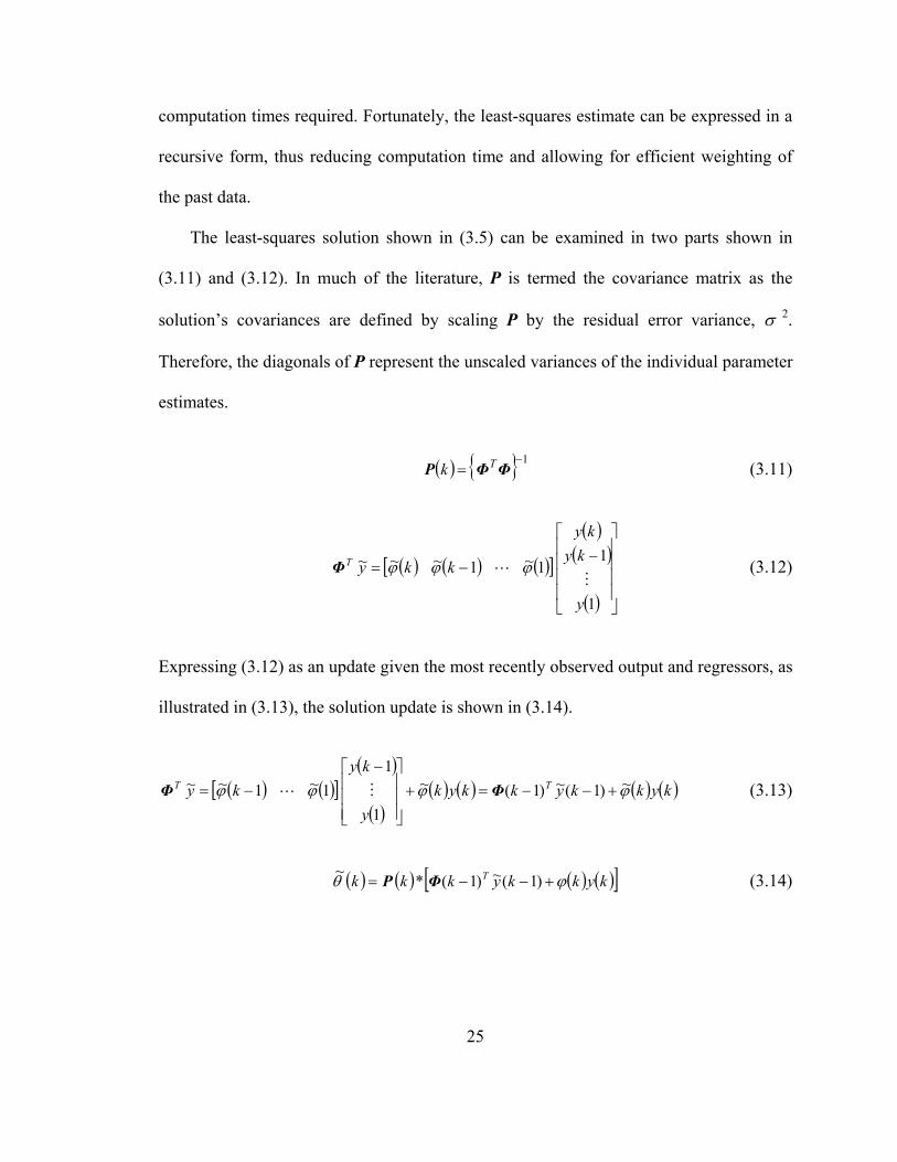
The least-squares solution shown in (3.5) can be examined in two parts shown in
(3.11) and (3.12). In much of the literature, P is termed the covariance matrix as the
solution’s covariances are defined by scaling P by the residual error variance, σ 2.
Therefore, the diagonals of P represent the unscaled variances of the individual parameter
estimates.
( ) { } 1−= ΦΦP Tk (3.11)
( ) ( ) ( )[ ]
( )( )
( ) ⎥⎥⎥⎥
⎦
⎤
⎢⎢⎢⎢
⎣
⎡−
−=
1
11~1~~~
y
kyky
kkyT
ML ϕϕϕΦ (3.12)
Expressing (3.12) as an update given the most recently observed output and regressors, as
illustrated in (3.13), the solution update is shown in (3.14).
( ) ( )[ ]( )
( )( ) ( ) ( ) ( )kykkykkyk
y
kyky TT ϕϕϕϕ ~)1(~)1(~
1
11~1~~ +−−=+
⎥⎥⎥
⎦
⎤
⎢⎢⎢
⎣
⎡ −−= ΦΦ ML (3.13)
( ) ( ) ( ) ( )[ ]kykkykkk T ϕθ +−−= )1(~)1(*~ ΦP (3.14)
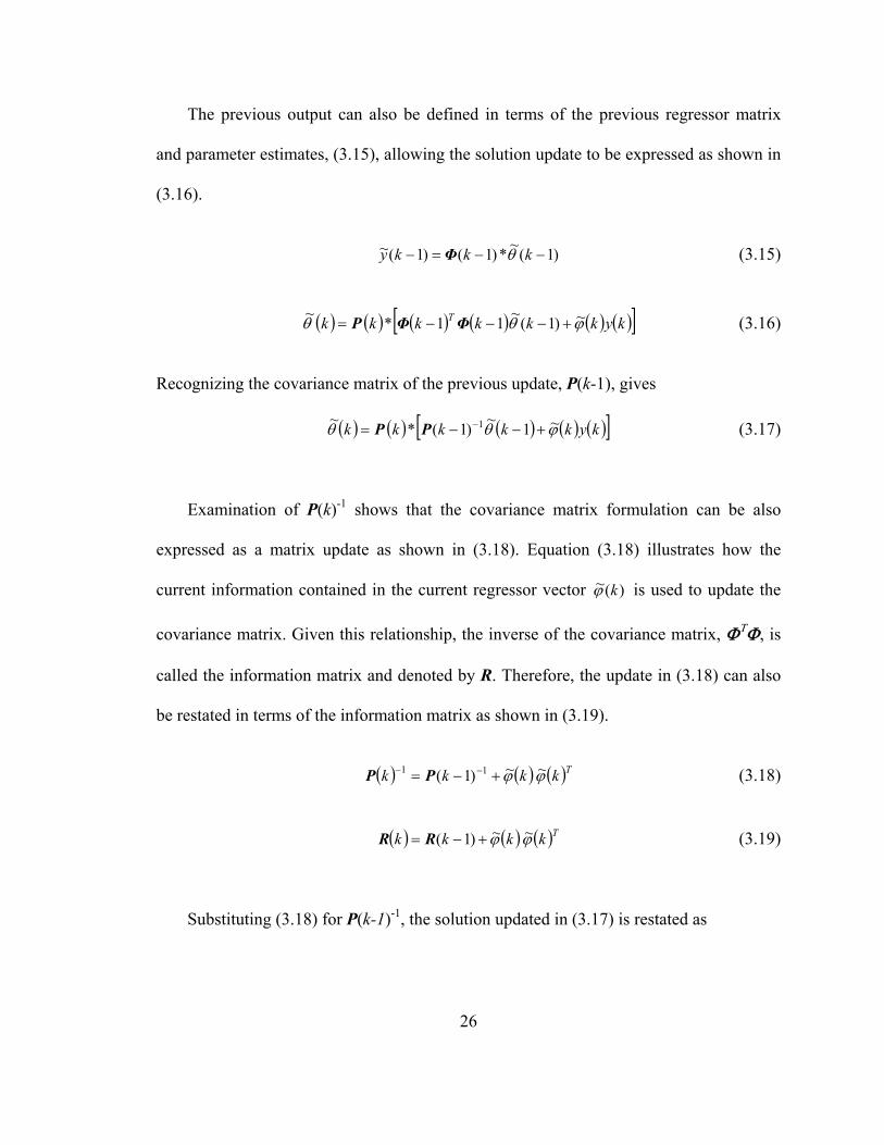
26
The previous output can also be defined in terms of the previous regressor matrix
and parameter estimates, (3.15), allowing the solution update to be expressed as shown in
(3.16).
)1(~*)1()1(~ −−=− kkky θΦ (3.15)
( ) ( ) ( ) ( ) ( ) ( )[ ]kykkkkkk T ϕθθ ~)1(~11*~+−−−= ΦΦP (3.16)
Recognizing the covariance matrix of the previous update, P(k-1), gives
( ) ( ) ( ) ( ) ( )[ ]kykkkkk ϕθθ ~1~)1(*~ 1 +−−= −PP (3.17)
Examination of P(k)-1 shows that the covariance matrix formulation can be also
expressed as a matrix update as shown in (3.18). Equation (3.18) illustrates how the
current information contained in the current regressor vector )(~ kϕ is used to update the
covariance matrix. Given this relationship, the inverse of the covariance matrix, ΦΤΦ, is
called the information matrix and denoted by R. Therefore, the update in (3.18) can also
be restated in terms of the information matrix as shown in (3.19).
( ) ( ) ( )Tkkkk ϕϕ ~~)1( 11 +−= −− PP (3.18)
( ) ( ) ( )Tkkkk ϕϕ ~~)1( +−= RR (3.19)
Substituting (3.18) for P(k-1)-1, the solution updated in (3.17) is restated as
27
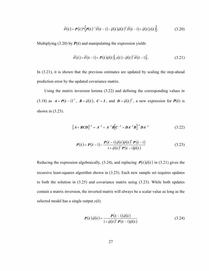
( ) ( ) ( ) ( ) ( ) ( ) ( ) ( ) ( )[ ]kykkkkkkkk T ϕθϕϕθθ ~1~~~1~*~ 1 +−−−= −PP . (3.20)
Multiplying (3.20) by P(k) and manipulating the expression yields
( ) ( ) ( ) ( ) ( ) ( ) ( ){ }1~~~1~~−−+−= kkkykkkk T θϕϕθθ P . (3.21)
In (3.21), it is shown that the previous estimates are updated by scaling the step-ahead
prediction error by the updated covariance matrix.
Using the matrix inversion lemma (3.22) and defining the corresponding values in
(3.18) as ( ) 11 −−= kPA , ( )kϕ~=B , IC = , and ( )Tkϕ~=D , a new expression for P(k) is
shown in (3.23).
[ ] [ ] 1111111 DABDACBAABCDA −−−−−−− ++=+ (3.22)
( ) ( ) ( ) ( ) ( ) ( )( ) ( ) ( )kkk
kkkkkk T
T
ϕϕϕϕ
~1~11~~11
−+
−−−−=
PPPPP (3.23)
Reducing the expression algebraically, (3.24), and replacing ( ) ( )kk ϕ~P in (3.21) gives the
recursive least-squares algorithm shown in (3.25). Each new sample set requires updates
to both the solution in (3.25) and covariance matrix using (3.23). While both updates
contain a matrix inversion, the inverted matrix will always be a scalar value as long as the
selected model has a single output y(k).
( ) ( ) ( ) ( )( ) ( ) ( )kkk
kkkk T ϕϕϕϕ ~1~1
~1~−+
−=
PPP (3.24)

28
( ) ( ) ( ) ( )( ) ( ) ( )
( ) ( ) ( )[ ]1~~~1~1
~11~~−−
−+
−+−= kkky
kkkkkkk T
T θϕϕϕ
ϕθθP
P (3.25)
The recursive least-squares solution is commonly expressed as three update calculations
as presented in (3.26) through (3.28). The matrix I in (3.28) is the p x p identity matrix.
As the vector ( )kL~ is used to scale the prediction error before updating the estimates, as
shown in (3.26), it is commonly termed the parameter update gain.
( ) ( ) ( ) ( ) ( ) ( ){ } 1~1~1~1~ −−+−= kkkkkkL T ϕϕϕ PP (3.26)
( ) ( ) ( )( )1~)(~)()(~1~~−−+−= kkkykLkk T θϕθθ (3.27)
( ) ( ) ( )( ) ( )1~~−−= kkkLIk T PP ϕ (3.28)
Before the first iteration, both the covariance matrix and unknown parameter guesses
in θ~ must be set to initial values. If prior knowledge concerning the parameters is not
available, the initial values of θ~ can be set to zero. As magnitudes in P(0) reflect the
level of confidence of the current solution, P(0) is typically initialized with large
diagonals values. The large covariance matrix results in large prediction errors gains as
defined by (3.26) and large step changes in the solution. Provided sufficiently exciting
data is available, the prediction error scaling will decrease along with the covariance
matrix as the estimates converge to a solution.
It is important to note that as the number of sample measurements goes to infinity,
the uncertainty in the parameter estimates will decrease as long as sufficiently exciting

29
measurements are available. This decrease in uncertainty is governed by the dyadic
product used to update the information matrix shown in (3.19). Therefore, both P(k) and
( )kL~ will either trend towards zero or remain unchanged depending on the level of
information contained in ( )kϕ~ . Furthermore, the covariance matrix will tend towards zero
even in the presence of Gaussian noise. However, the decreasing gain also means the
method will become increasingly less sensitive to prediction errors. As a consequence the
RLS method will eventually be unable to follow or track parameter changes. This is
easily demonstrated by introducing a zero matrix for P(k) in (3.21). Clearly in this case,
updates to the parameter estimates will not occur regardless of the prediction errors.
To permit tracking parameter changes it is necessary to discount or forget past data.
This can be done through an exponential forgetting factor λ [56], where 0 < λ ≤1 and λ=1
corresponds to recursive least-squares without any discounting. The effect of including
the forgetting factor in the solution is shown through the updated cost function in
(3.29). For values of λ less than 1, the past residuals are exponentially decreased by a rate
determined by λ until their influence is negligible, thus emphasis is placed on recent
measurements. Therefore, inclusion of the forgetting factor in the least-squares solution is
equivalent to a weighted least-squares formulation.
( ) ( ) ( )( )∑+−=
− −=k
kmi
Tik iyiJ1
2~~21 θϕλθ (3.29)
The discounting of past information can also be expressed in terms of the
information matrix update given in (3.30). During each update of the information matrix,
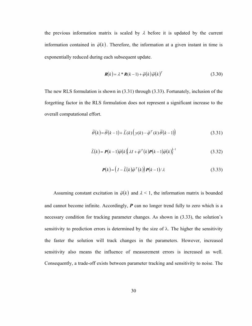
30
the previous information matrix is scaled by λ before it is updated by the current
information contained in ( )kϕ~ . Therefore, the information at a given instant in time is
exponentially reduced during each subsequent update.
( ) ( ) ( )Tkkkk ϕϕλ ~~)1(* +−= RR (3.30)
The new RLS formulation is shown in (3.31) through (3.33). Fortunately, inclusion of the
forgetting factor in the RLS formulation does not represent a significant increase to the
overall computational effort.
( ) ( ) ( )( )1~)(~)()(~1~~−−+−= kkkykLkk T θϕθθ (3.31)
( ) ( ) ( ) ( ) ( ) ( ){ } 1~1~~1~ −−+−= kkkIkkkL T ϕϕλϕ PP (3.32)
( ) ( ) ( )( ) ( ) λϕ /1~~−−= kkkLIk T PP (3.33)
Assuming constant excitation in ( )kϕ~ and λ < 1, the information matrix is bounded
and cannot become infinite. Accordingly, P can no longer trend fully to zero which is a
necessary condition for tracking parameter changes. As shown in (3.33), the solution’s
sensitivity to prediction errors is determined by the size of λ. The higher the sensitivity
the faster the solution will track changes in the parameters. However, increased
sensitivity also means the influence of measurement errors is increased as well.
Consequently, a trade-off exists between parameter tracking and sensitivity to noise. The

31
selection of λ will therefore need to be performed on an ad-hoc basis to ensure necessary
tracking capabilities are provided without undue sensitivity to noise.
The discounting rate can be selected based on the desired exponential-decay time
constant, T0, and the time between measurements, T, using the relationship shown in
(3.34). This approach requires prior knowledge about the nature of the parameter changes
and acceptable tracking rates. For instance, approximately four to five time constants are
required to converge to the new solution after an abrupt step change in a parameter.
Therefore, lower values of λ should be expected. However, in the case of slowly varying
parameter changes, larger values of λ will provide less sensitivity to measurement noise
while retaining the ability to track the parameter changes. As model-based diagnostic and
prognostic evaluations are not meant to facilitate fast acting protection, selecting λ as
0.99 or higher is expected to provide sufficient tracking capabilities.
( )λln−=
TTo (3.34)
It can be shown the time constant in terms of the number of samples N is
approximated by (3.35) for values of λ close to one. One study states that (3.35)
represents the rectangular sliding window size necessary to approximate the solution
provided by the exponentially discounted window [58]. However, a common rule of
thumb is to approximate the “memory” of the estimator as twice the time constant given
in (3.35) [56].
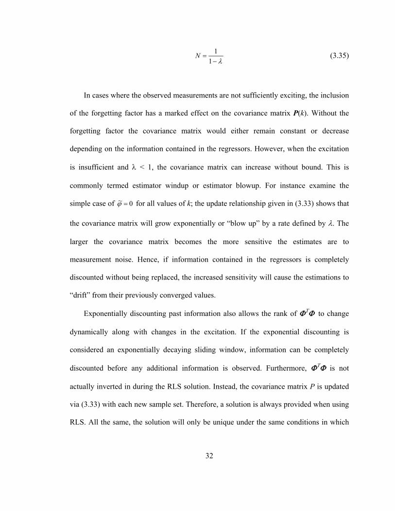
32
λ−
=1
1N (3.35)
In cases where the observed measurements are not sufficiently exciting, the inclusion
of the forgetting factor has a marked effect on the covariance matrix P(k). Without the
forgetting factor the covariance matrix would either remain constant or decrease
depending on the information contained in the regressors. However, when the excitation
is insufficient and λ < 1, the covariance matrix can increase without bound. This is
commonly termed estimator windup or estimator blowup. For instance examine the
simple case of 0~ =ϕ for all values of k; the update relationship given in (3.33) shows that
the covariance matrix will grow exponentially or “blow up” by a rate defined by λ. The
larger the covariance matrix becomes the more sensitive the estimates are to
measurement noise. Hence, if information contained in the regressors is completely
discounted without being replaced, the increased sensitivity will cause the estimations to
“drift” from their previously converged values.
Exponentially discounting past information also allows the rank of ΦΤΦ to change
dynamically along with changes in the excitation. If the exponential discounting is
considered an exponentially decaying sliding window, information can be completely
discounted before any additional information is observed. Furthermore, ΦΤΦ is not
actually inverted in during the RLS solution. Instead, the covariance matrix P is updated
via (3.33) with each new sample set. Therefore, a solution is always provided when using
RLS. All the same, the solution will only be unique under the same conditions in which

33
the covariance matrix is non-singular. Obviously, these excitation properties of RLS with
exponential forgetting are a concern when the excitation is intermittent.
When applying recursive solutions the excitation condition is known as the
persistence of excitation. Persistence of excitation simply means that the signal contains
sufficient excitation to keep the information matrix from becoming singular over infinite
time. A signal u is termed persistently exciting (PE) of order n if it results in the n x n
ΦΤΦ matrix being full rank. As the information matrix’s dimension equals the number of
unknown parameters, a unique solution is only determined when the signal’s PE equals
the number unknown parameters. It is important to note that the number of unknown
parameters directly determines the required level of excitation.
Excitation in the regressors can be examined by the dynamic content contained in the
observed waveforms. For example, it can be shown that a step function is PE order of 1
while a signal containing k sinusoids is PE of order 2k [56]. Therefore, a possible test for
sufficient excitation might be to use Fourier analysis to determine the number of nonzero
sinusoids in the measurements and compare this to the number of parameters to be
estimated. Another test would be to determine the rank of the information matrix.
Parameters could then be updated only if the excitation is sufficient to estimate all the
modeled parameters. Such methods are known in the controls literature as conditional
updating methods.
A rank deficient covariance matrix indicates that incoming information is not equally
distributed among the parameter space. While some dimensions of the parameter space
may be excited, or contain new data, other dimensions may not. Conditional updating
34
methods do not take advantage of the available information as they only update the
covariance matrix when information exists in all dimensions of the parameter space. If
the covariance matrix is not bounded, however, estimator windup will occur in the
unexcited region of the parameter space. A method which bounds the covariance matrix
in all dimensions while still updating the excited regions represents a more efficient use
of the available information.
3.2.1. DIRECTIONAL FORGETTING
Numerous methods have been proposed to address covariance windup, typically
through enforcement of some type of upper bound on the covariance matrix. One of the
earliest solutions varies the forgetting factor as a function of the prediction error and the
excitation [59]. During periods of low excitation, when limited information is being
received, the forgetting factor is forced towards unity to limit the loss of past information
and bound the covariance matrix. In [60] resetting of the covariance matrix during low
periods of excitation was proposed. However, both variable forgetting (VF) and resetting
methods are applied equally in all directions of the parameter space regardless of the
distribution of information.
In contrast, directional forgetting (DF) methods only discount past data in those
directions in which newer data is available. This means the parameters associated with
newer information can be updated without causing estimator windup to occur in the other
parameters. Initial methods of direction forgetting were given in [61, 62]. However, these
methods did not bound the covariance matrix from below [63-65]. Consequently, the

35
originally proposed directional forgetting method’s covariance matrix could trend fully to
zero causing in the method to lose its ability to track parameter changes.
Analogous to directional forgetting, a method was proposed in [66] which uses the
eigenvectors of the information matrix to determine the directional distribution of the
information. Individual forgetting factors were then assigned to the eigenvalues to ensure
upper and lower bounds were enforced upon the covariance matrix. As individual
forgetting factors were allocated to each eigenvector (dimension), discounting of the past
information was performed selectively in each direction of the parameter space.
Accordingly, this method was termed “selective” forgetting (SF) and was shown to be
effective when estimating time-varying parameters which vary at different rates [67]. As
the eigen-structure must be calculated for every new sample, a good deal of computation
effort was required by the method.
A new directional forgetting algorithm was proposed in [68, 69] that determines
what dimensions of the parameter space can be safely discounted through decomposition
of the information matrix. This method has been shown to have the benefit of bounding
the covariance matrix from above (preventing estimator windup) and below (preventing
loss of tracking). Additionally, the algorithm does not require calculation of the
eigenvalues and eigenvectors as performed by the SF method. The algorithm decomposes
the information matrix into two parts as shown in (3.36), R1(k-1) which contains the
information orthogonal to the new information and R2(k-1) which contains the
information projected onto the parameter space of the current excitation. Exponential
forgetting is only applied to the portion of the information matrix in the same parameter
36
space as the current excitation. Consequently, information associated with a particular
parameter is only discounted when newer information is available. This is highly
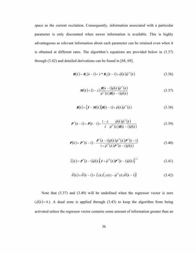
advantageous as relevant information about each parameter can be retained even when it
is obtained at different rates. The algorithm’s equations are provided below in (3.37)
through (3.42) and detailed derivations can be found in [68, 69].
( ) ( ) ( ) ( ) ( )kkkkk Tϕϕλ ~~1*1 21 +−+−= RRR (3.36)
( ) ( ) ( ) ( ) ( )( ) ( ) ( )kkk
kkkk T
T
ϕϕϕϕλ ~1~~~11
−−
−=R
RM (3.37)
( ) ( )[ ] ( ) ( ) ( )kkkkk Tϕϕ ~~1 +−−= RMIR (3.38)
( ) ( ) ( ) ( )( ) ( ) ( )kkk
kkkk T
T
ϕϕϕϕ
λλ
~1~~~111*
−−
+−=−R
PP (3.39)
( ) ( ) ( ) ( ) ( ) ( )( ) ( ) ( )kkk
kkkkkk T
T
ϕϕϕϕ
~1~11~~11 *
***
−+−−
−−=P
PPPP (3.40)
( ) ( ) ( ) ( ) ( ) ( ){ } 1** ~1~~1~ −−+−= kkkkkkL T ϕϕϕ PIP (3.41)
( ) ( ) ( )( )1~)(~)()(~1~~−−+−= kkkykLkk T θϕθθ (3.42)
Note that (3.37) and (3.40) will be undefined when the regressor vector is zero
( ( ) 0~ =kϕ ). A dead zone is applied through (3.43) to keep the algorithm from being
activated unless the regressor vector contains some amount of information greater than an

37
assumed noise level α. When the test in (3.43) is satisfied, the DF method is altered by
(3.44) and (3.45). Therefore, discounting will not occur when the measurements contain
only noise.
( ) αϕ ≤k~ (3.43)
0)( =kM (3.44)
( ) ( )11* −=− kk PP (3.45)
3.2.2. VARIABLE DIRECTIONAL FORGETTING
An interesting design consideration arises when considering long-term passive
monitoring requirements. Specifically, how much weight should be applied to older data
when significant gaps exist between periods of sufficient excitation or when significantly
abrupt parameter changes occur? Suppose that after converging to the “true” solution,
new information about a parameter is unavailable for a long period of time. During this
time the actual value of the parameter varies slowly but significantly from the last
parameter estimate. When the excitation returns to that parameter space the change will
appear as an abrupt step change in the estimation and the estimates will be biased until
the past information is replaced.
As past information is discounted only as new information becomes available, the
actual rate at which past data is discounted is a function of λ as well as a function of the
rate at which newer information becomes available. Therefore, it is more convenient to

38
consider the retained information in terms of the equivalent memory size as defined
(3.35) versus a time constant. For example, an equivalent memory size of 200 data points
results when λ is 0.99. When an abrupt parameter change occurs, 200 new relevant data
points will need to be observed before the all past information is discounted. As a result,
directional forgetting may exhibit slower parameter tracking capabilities compared to
standard exponential forgetting. However, this assumes the excitation is sufficient to
overcome estimator windup and the influence of measurement errors when using
standard exponential forgetting.
One option to account for abrupt parameter changes is to dynamically alter the
memory size by adjusting λ. The amount of past data retained in the calculations is then
determined by how well the model predicts current observations. When the prediction
error (3.46) is larger than a set tolerance, λ is set to a low value then exponentially
increased. As the information which triggered the high prediction error may not exist in
subsequent observation, λ is exponentially increased back to its original set-point. This
allows increased discounting to occur in any parameter space associated with incoming
information.
( ) ( ) ( ) ( ){ }1~~ −−= kkkyk T θϕε (3.46)

39
3.2.3. COVARIANCE RESETTING
Another option is to simply remove all the past data when a large abrupt step-change
occurs. Given indications that the model is inadequately predicting the observations (i.e.
the error in (3.46) is larger than a set tolerance) the covariance matrix P could be reset to
its initial value P=α*I; where α is a large scalar value and I is the identity matrix.
Resetting the covariance matrix indicates that there is little confidence in the current
estimations and essentially restarts the estimation process using the current parameter
estimates as the initial starting point. When P (and consequently R) is reset the past
information for every parameter is lost, and all of the parameters estimates will deviate
from their previously converged values until sufficient excitation for each parameter is
again obtained. Obviously, covariance resetting represents a drastic response. In cases
where the excitation is extremely intermittent, resetting the covariance matrix will keep
past data from biasing the estimates over longer periods of time.
Other system identification methods and methods to prevent estimator windup exist
and a detailed examination of these methods can be found in [55]. Determination of
which method to use should be based on the complexity of the model and the expected
excitation. A summary of the various recursive estimation variations discussed here are
presented in Table 3-1 along with a brief discussion of potential applications as well as
pros and cons.
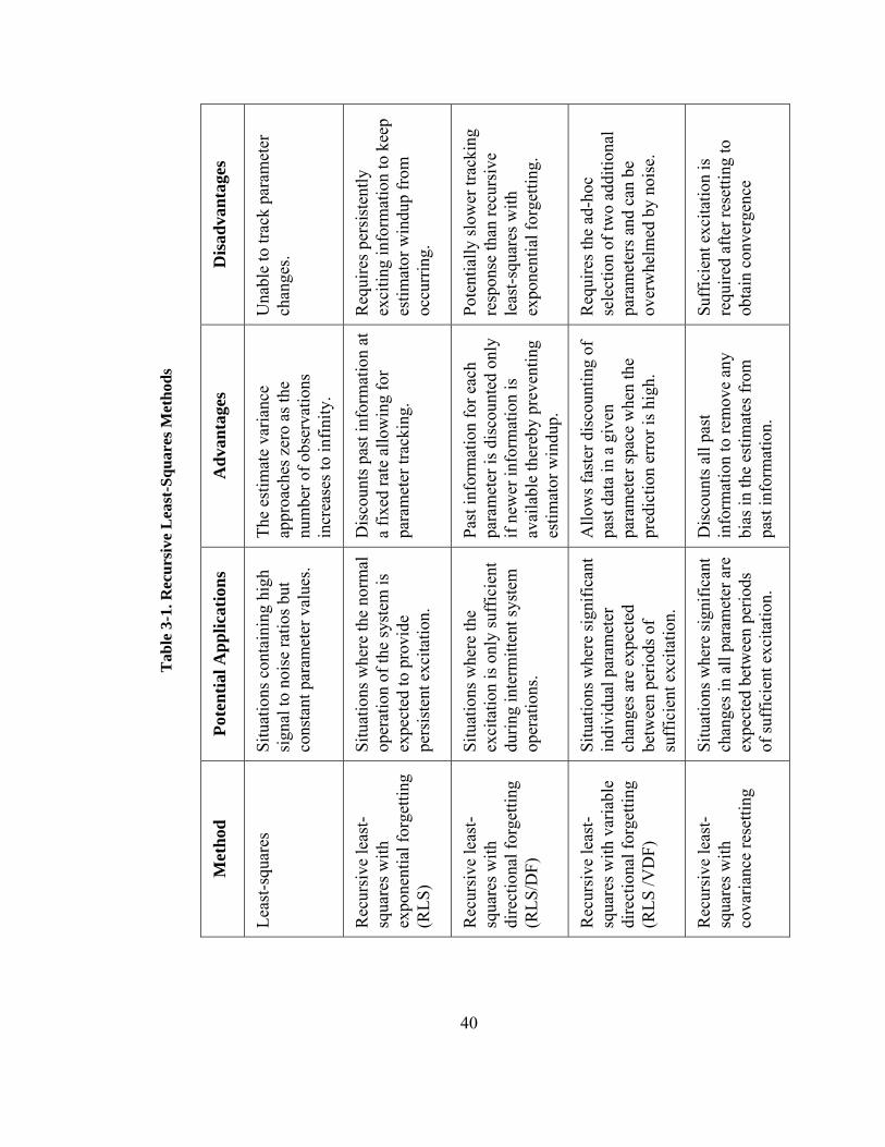
40
Dis
adva
ntag
es
Una
ble
to tr
ack
para
met
er
chan
ges.
Req
uire
s per
sist
ently
ex
citin
g in
form
atio
n to
kee
p es
timat
or w
indu
p fr
om
occu
rrin
g.
Pote
ntia
lly sl
ower
trac
king
re
spon
se th
an re
curs
ive
leas
t-squ
ares
with
ex
pone
ntia
l for
getti
ng.
Req
uire
s the
ad-
hoc
sele
ctio
n of
two
addi
tiona
l pa
ram
eter
s and
can
be
over
whe
lmed
by
nois
e.
Suff
icie
nt e
xcita
tion
is
requ
ired
afte
r res
ettin
g to
ob
tain
con
verg
ence
Adv
anta
ges
The
estim
ate
varia
nce
appr
oach
es z
ero
as th
e nu
mbe
r of o
bser
vatio
ns
incr
ease
s to
infin
ity.
Dis
coun
ts p
ast i
nfor
mat
ion
at
a fix
ed ra
te a
llow
ing
for
para
met
er tr
acki
ng.
Past
info
rmat
ion
for e
ach
para
met
er is
dis
coun
ted
only
if
new
er in
form
atio
n is
av
aila
ble
ther
eby
prev
entin
g es
timat
or w
indu
p.
Allo
ws f
aste
r dis
coun
ting
of
past
dat
a in
a g
iven
pa
ram
eter
spac
e w
hen
the
pred
ictio
n er
ror i
s hig
h.
Dis
coun
ts a
ll pa
st
info
rmat
ion
to re
mov
e an
y bi
as in
the
estim
ates
from
pa
st in
form
atio
n.
Pote
ntia
l App
licat
ions
Situ
atio
ns c
onta
inin
g hi
gh
sign
al to
noi
se ra
tios b
ut
cons
tant
par
amet
er v
alue
s.
Situ
atio
ns w
here
the
norm
al
oper
atio
n of
the
syst
em is
ex
pect
ed to
pro
vide
pe
rsis
tent
exc
itatio
n.
Situ
atio
ns w
here
the
exci
tatio
n is
onl
y su
ffic
ient
du
ring
inte
rmitt
ent s
yste
m
oper
atio
ns.
Situ
atio
ns w
here
sign
ifica
nt
indi
vidu
al p
aram
eter
ch
ange
s are
exp
ecte
d be
twee
n pe
riods
of
suff
icie
nt e
xcita
tion.
Situ
atio
ns w
here
sign
ifica
nt
chan
ges i
n al
l par
amet
er a
re
expe
cted
bet
wee
n pe
riods
of
suff
icie
nt e
xcita
tion.
Tab
le 3
-1. R
ecur
sive
Lea
st-S
quar
es M
etho
ds
Met
hod
Leas
t-squ
ares
R
ecur
sive
leas
t-sq
uare
s with
ex
pone
ntia
l for
getti
ng
(RLS
)
Rec
ursi
ve le
ast-
squa
res w
ith
dire
ctio
nal f
orge
tting
(R
LS/D
F)
Rec
ursi
ve le
ast-
squa
res w
ith v
aria
ble
dire
ctio
nal f
orge
tting
(R
LS /V
DF)
Rec
ursi
ve le
ast-
squa
res w
ith
cova
rianc
e re
setti
ng
41
3.2.4. MULTIVARIABLE SOLUTIONS
The presented recursive formulations are applicable to models where a single output
is specified. However, the formulations are also applicable to models with multiple inputs
and multiple outputs (MIMO models). One approach is to divide the model into
individual multiple input single output (MISO) models which are fitted to the data
separately using the previously derived techniques. Conversely, it can be recognized that
the multiple inputs are shared by each MISO model signifying that the regressors are
shared by each model. If each model is weighted equally in the overall cost function, only
(3.31) must be updated to account for the increased dimensions as denoted in (3.47)
where θ(k) contains multiple parameter vectors. For m outputs, θ(k) is a p x m matrix and
( )ky~ is a 1 x m vector containing the output variables.
( ) ( ) ( )( )1~~~1 −−+−= k(k)(k)y(k)Lkk T θθθ ϕ (3.47)
While the multivariable formulation appears more efficient than solving the
individual MISO models, the parameter vectors composing θ(k) are still independent
from each other. The same unknown modeled in multiple locations of θ(k) will have
multiple independent solutions. Additionally, the multivariable solution requires that each
of the MISO models share the same regressors. Consequently, the MIMO model may not
represent the most optimal form to estimate the desired parameters. However, the
multivariable models should be considered in cases where these limitations are not a
significant factor.

42
3.3. MODEL AND PARAMETER VALIDATION
As previously noted, the RLS algorithm always provides a solution regardless of the
current or past level of excitation. Because the excitation is not artificially regulated,
there is no assurance that the current estimation set is representative of the true
parameters. More specifically, without sufficient past excitation the collected information
may not be adequate for satisfactory convergence. In response, statistical inference
measures were implemented to validate or judge the level of confidence in the parameter
estimates. Additional tests are also introduced to quantify the regressors’ linear
independence. Finally, model validation through residual analysis is discussed.
The statistical measures will be useful in the diagnosis and prognosis sections of the
condition monitor and will be stored along with the estimates, θ~ , as shown in Figure 3-1.
Both the unknown estimates and the statistical measures are determined using the
sampled measurements (v1(k), i1(k), ...) which are filtered and normalized (v1 (k)*, i1(k)*,
...) before applying the solution method. The stored statistical measures include the
prediction error, ε, determined by the solution method as well as the variance of the
unknown parameter estimates, σ 2, and the calculated confidence intervals (CI) which are
determined from the covariance matrix, P, and ε. Other forms of expressing the estimates
accuracy, such as margins or error, could be stored instead of the confidence intervals.

43
Normalization &
Filtering
Recursive Parameter Estimation
w/ Forgetting
Statistical Evaluations
Analogue to Digital Conversion
Model-BasedDiagnosis
andPrognosis
v1(k), i1(k), ….
2, CI
v1(k)*, i1(k)*, ….
P
θ~
Figure 3-1. Condition Monitor Parameter Estimation and Validation Block
3.3.1. MARGINS OF ERROR
Statistical inference about the parameter estimates requires knowledge about the
estimate variance. As previously noted, the actual matrix of covariances for the parameter
estimates is found by scaling P by noise variance as indicated in (3.48).
( ) P2cov σθ = (3.48)
While P is readily available from the recursive least-squares formulations, the error or
noise variance, σ 2, is not. Revisiting (3.1), σ 2 is the variance of the residuals between the
true and predicted output values for a particular estimated parameter set. One possible
approach is to recalculate the residual errors for each new parameter solution and re-

44
estimate the variance. This approach represents a large computation burden and requires
the storage of a large amount of past regressor data. If the parameters are assumed
constant, both the residual and prediction error variances are equal to the noise variance.
Thus, σ 2 can be approximated using the prediction error instead.
The sample variance of the prediction error can be estimated using (3.49).
( ) ( ) ( ) ( )[ ]∑−
−=N
k
T NkkyN
N1
2 ~*~1ˆ θϕσ (3.49)
Taking into account that the number of samples N used to estimate the parameters is
defined by (3.35), the sample variance can be rewritten as shown in (3.50).
( ) ( ) ( ) ( )[ ] ( ) ( )[ ]∑−
−
−+−=1
1
22 1~*~ˆN
k
T NNkkyN ελθϕσ (3.50)
When the parameter estimates θ(N) are constant over a sufficient period of time, the
predictions errors, ε, over this period are good predictors of the residuals. In this case,
(3.50) can be restated in a recursive form with the past estimates discounted in the same
manner as the parameter estimates. Therefore, the approximation of σ 2 can change over
time in a manner similar to the parameter estimations.
( ) ( ) ( ) ( )[ ]NNN 222 11ˆˆ ελσλσ −+−= (3.51)
Furthermore, it was shown in [70, 71] that the estimations of the residual from the
prediction errors could be improved by accounting for the past information contained in
45
P. The final version of the residual variance estimate is given in (3.52). The forgetting
factor used in (3.52) is the same value used to discount the observed information.
( ) ( ) ( ) ( ) ( ) ( )[ ] ( ) ( ) ( )[ ]1~~*~~1*11ˆˆ 22 −−−−+−= kkkykkkkk TT θϕϕϕλσλσ P (3.52)
The noise variance estimate of (3.52) can be used in (3.48) to estimate the variance
and covariance values necessary to determine the confidence intervals. Assuming the
error is zero mean white noise and insignificant correlation between the parameters, the
100(1-α)% confidence interval for each parameter can be estimated using (3.53), where n
and p are again the number of observations and unknown parameters respectively and Pjj
is the jth diagonal term in the covariance matrix. The parameter estimations follow a chi-
squared distribution [72] and the Student-t value with n-p degrees of freedom is chosen to
scale the interval. Recalling that the number of observations used by the calculations is
governed by the forgetting factor, the value of n is approximated as five times the
memory size defined in (3.35).
( ) jjj Ppnt σαθ ˆ*;2/1 −−± (3.53)
However, the univariate confidence interval in (3.53) only addresses the hypothesis
that a particular parameter’s true value is contained within the interval. A more
conservative hypothesis is whether all the intervals simultaneously contain their
respective true values. In other words, what confidence space simultaneously contains the
model’s true parameters for a specified confidence level? Bonferroni confidence intervals
46
are the simplest simultaneous test to account for the joint evaluation of multiple
parameters as this approach divides the confidence level (1-α) by the number of
parameters to be estimated, as seen in (3.54). Accordingly, the Bonferroni confidence
intervals are easily calculated and provide a conservative interval range. The benefit of
the Bonferroni confidence intervals as applied to online synchronous machine parameter
estimation was recently examined in [73].
jjj Ppnp
t σαθ ˆ*;2/1⎟⎟⎠
⎞⎜⎜⎝
⎛−
−± (3.54)
The added/subtracted value in (3.54) is termed the margin of error which is often
reported in lieu of an actual confidence interval. During the online application, the
margins of error could be tested against preset tolerances to decide whether an estimate is
sufficiently accurate to warrant action or storage for later evaluation. However, in order
for the confidence intervals to accurately reflect upon the accuracy of the estimations, the
assumption that the residuals are white noise must still be satisfied.
3.3.2. MULTICOLLINEARITY TESTS
It was previously shown that identifiability is determined by the singularity or non-
singularity of the information matrix, R = ΦΤΦ. Intrinsically, singularity of the matrix is
determined by the linear independence of the regressors which form the columns of Φ.
Therefore, the level of excitation is decreased whenever linear dependence or
multicollinearity exists between the regressors. A multiple regression statistic known as
47
the variance inflation factor (VIF) is a commonly used indicator of linear dependence
between multiple variables. Typically, the VIF is defined in the form shown in (3.55)
where the jth column of Φ is denoted by jΦ~ .
( )j
Tj
jj VIFΦΦ
= ~~*var2σθ (3.55)
Revisiting (3.7), it can be seen that j
Tj ΦΦ ~~ is the jth diagonal of the information
matrix R. Additionally, a parameter estimate’s variance is given by the jth diagonal of
(3.48). Therefore, (3.55) can be simplified to the form shown in (3.56). Recalling that P
and R are inverses, the VIF reflects the degree in which a diagonal in P is increased due
to nonzero off-diagonals in the information matrix. For example when R is diagonal, Rjj
and Pjj are direct inverses and the value of VIF must be one. Conversely when perfect
linear dependence exists between the regressors, both Pjj and VIFj are infinite.
jj
jjj RVIFP 1*= (3.56)
While the variance inflation factor is a useful diagnostic, the square root of the VIF
is more functional because it directly specifies how the standard error, and consequently
the confidence interval, is enlarged by the multicollinearity. In [74] this value is termed
the standard-error inflation factor (SIF) and its calculation is given in (3.57). An obvious

48
benefit of the SIF is the required data is already generated by the recursive algorithms.
Storage of the SIF will be a valuable offline tool for evaluating a model’s effectiveness.
jjjjj RPSIF = (3.57)
While the SIF is a good indicator of multicollinearity, it does not indicate which
regressor terms are strongly correlated. While examining the model identifiability
requirements, collinearities between the regressors are established through examination
of the correlation matrix. The correlation matrix is determined by scaling the entries in P
by the associated standard deviations as indicated in (3.58). The off-diagonal entries of
the correlation matrix indicate the level of correlation that exists between the regressors;
values close to one indicate a strong positive correlation while values close to negative
one indicate a strong negative correlation.
⎥⎥⎥⎥⎥⎥
⎦
⎤
⎢⎢⎢⎢⎢⎢
⎣
⎡
⎥⎥⎥⎥⎥⎥
⎦
⎤
⎢⎢⎢⎢⎢⎢
⎣
⎡
=
pppp P
PP
P
PP
1
1
1
**
1
1
1
22
11
22
11
OOPC (3.58)
3.3.3. RESIDUAL ANALYSIS
Whether the chosen model sufficiently represents the true characteristics of the
device is a subjective question of validation. A simple evaluation is whether the estimated
parameters are physically viable. For example, a negative resistance model would be a

49
red flag to revisit the selected model. Another useful validation test is to inspect the
confidence intervals to determine if a modeled parameter could be removed from the
model. For example, a confidence interval which consistently crosses zero might indicate
that a variable could be removed from the model. However, an unmodeled variable could
bias the estimates when conditions change. This selection is often described as a trade off
between model flexibility and parsimony [55]. Simply put, the model can be flexible and
better at explaining more of the dynamics (reducing bias), or the number of parameters
can be reduced which typically reduces the variance (fewer parameters reduces the
potential for multicollinearity). In fact, large standard deviations may be a sign of an
over-defined model.
As previously noted, the confidence intervals proposed in the previous section are
dependent on the residuals being zero mean white noise. Otherwise, the residuals contain
additional content which could be modeled. Consequently, non-white residuals are a sign
of inaccuracy in the model structure. Model validation is a process that is best achieved
offline when necessary corrections are easier to recognize and implement. Some general
solutions to non-white residuals are:
1. Modify the model structure to account for any unmodeled physical dynamics,
2. Modify the model and/or solution method to include an error model (i.e.
extended least squares),
3. Filter the extra dynamic content, or
4. Deem the bias to be at an acceptable level for the given application.

50
While there are numerous tests which could be applied to evaluate the residuals’
whiteness (autocorrelation, Durbin-Watson test, etc.) each test requires significant
calculations and data storage to recalculate the residuals at each time step. Moreover,
temporary dynamic residual content arising from parameter changes and subsequent
tracking could also be interpreted falsely by an automated test. The proposed online
model validations are limited to the parameter feasibility and confidence intervals
mentioned earlier. However, the historical data portion of Figure 1-1 could be used to
periodically generate whiteness test reports if desired.
Assuming that a sufficiently representative model is utilized, analysis of the residuals
between the measured and predicted output could provide valuable diagnostic
information. For example, a model reference approach as shown in Figure 2-1 could be
used to indicate when the device operates in a manner which cannot be accounted for by
the model. Therefore, storage and evaluation of the prediction error in (3.46) should be
considered along with the parameter estimates.
3.4. MEASUREMENT NOISE
Any parameter estimate cannot be more accurate than the data used in the
approximation. Increasing the memory size can reduce the influence of noise but results
in slower tracking of time-varying parameters. Measurement noise also influences the
confidence interval estimates by increasing the noise variance in (3.48). To some extent,
the amount of measurement noise is determined by the method used to collect the sample

51
data. Hence, common filtering and quantization design criteria which affect the accuracy
of the estimates require examination.
3.4.1. QUANTIZATION AND SAMPLING RATE
As shown in Figure 1-1, the proposed parameter online diagnostic monitor requires
discrete measurements provided by an analog-to-digital converter. Assuming the analog
signal can take on any value, the resulting quantization error is typically considered
uniformly distributed white noise with the probability density shown in (3.59). The limits
of the uniform distribution are defined by the incremental step size q used by the A/D
process while the step size is determined by the number of bits, n, used in the A/D
process and the full scale over which the analog values are discretized minmax rrr −=Δ .
This relationship is illustrated in (3.60). While the actual noise variance σ 2 is dependent
on many factors, in general larger measurement noise will result in larger noise variance.
Therefore, the noise variance, and hence the estimate variance, can be improved by
increasing the number of bits used in the A/D process.
( ) ( )⎪⎭
⎪⎬⎫
⎪⎩
⎪⎨⎧ ≤≤−
=otherwise
qkeqkep
022; (3.59)
n
rq
2
Δ= (3.60)

52
The sampling rate of the A/D conversion also influences the estimates by determining
the content contained in the sample observations. To keep from aliasing the sample data
the sampling frequency should be twice the highest expected frequency. As the frequency
content cannot be known ahead of time, anti-aliasing filters are necessary to ensure
frequency content above the Nyquist frequency is not contained in the sample data.
Potentially, any sampling rate could then be implemented as long as sufficient filtering is
applied, though sampling at lower frequencies will potentially capture less information.
In general, the measurements should be sampled as fast and with as much accuracy as
hardware will allow.
3.4.2. FILTERING
As noted in the previous sections, filtering is an important component of the
parameter estimation procedure. Proper filter selection prevents aliasing and reduces the
noise variance. However, identical filters must be applied to every measurement to keep
from artificially biasing the input-output relationship. While filtering can be viewed as
biasing estimates toward a particular frequency range, it can be shown that when identical
filters are applied to each measurement the input-output relationships are unaltered.
Consequently, filter design issues such as ripple in the pass band are not a significant
concern. Therefore, filters characterized by sharper transitions between the passband and
stopbands, such as high order Chebyshev filters, can be used.
Given some of the gathered information may result from transient events whose
frequency content cannot be predicted, sampling at a high rate alone cannot guarantee

53
aliasing will not occur. Thus, anti-aliasing filters must be implemented by analog devices
before the measurements are fed into the A/D device. However, additional digital
filtering can be applied as needed. For example, digital filters may be needed to remove
unmodeled content from the observations not removed by the anti-aliasing filters. This is
an important design consideration as any unmodeled content will bias the parameter and
confidence interval estimates. Therefore, filter design must be performed for each
monitoring device considering the model’s dynamic characteristics.
3.5. NORMALIZATION
Measured input-output data and the parameters estimates themselves will typically
exist in different scales. Significantly dissimilar scales are a concern as they can result in
numerical errors during the estimation process. One solution is to normalize or per-
unitize the input-output data, and consequently the estimations, by scaling the data using
carefully chosen bases. Each data type (voltage, current, time, etc.) shares a single base
value and any physical relationships between these data types must be enforced.
In the time domain the per-unit bases for the physical or electrical parameters can be
expressed in terms of v, i, and t [75]. The relationships between v-i-t bases and the bases
representing the physical parameters are provided in Table 3-2. It is necessary that three
of the bases shown in Table 3-2 be specified. All unspecified bases will be determined
using the relationships given in the fourth column of Table 3-2. However, care must be
taken to ensure the selected bases fully span all three dimensions of v-i-t. Other bases
could be introduced given additional measurement types and model configurations.

54
Table 3-2. Time Domain Per-Unit Base Relationships
Base Quantity Units v-i-t Relationship
Vbase Voltage Voltage (v) v Ibase Current Amperes (A) i tbase Time Seconds (s) t Sbase Power Volt-Amperes (VA) vi Rbase Resistance Ohms (Ω) v/i Lbase Inductance Henries (H) vt/i Cbase Capacitance Farads (F) it/v
Proper base selection is essential when utilizing RLS with directional forgetting.
Projecting the information matrix onto a parameter space which is overly skewed will
result in numerical errors that influence the convergence and tracking abilities of the
method. Specifically, past information associated with the smaller scaled regressors will
not accurately be projected onto the space parallel to the incoming information. Hence,
discounting of past information associated with these regressors will be limited. As such,
base selection can intentionally or inadvertently influence parameter tracking when
directional forgetting is used.
55
CHAPTER 4
TWO-CONDCUTOR MODELS
As mentioned in section 3.1, parameter identifiability is dependent on the solution
method, the model structure, and the measured input-output data. Model-based
diagnostics of network health is therefore reliant upon the available measurements and
selected model as much as the estimation algorithm. In this chapter estimation of two
conductor electrical parameters is evaluated using time-domain measurements. The
identifiability requirements of multiple conductors using time-domain measurements are
subsequently evaluated in Chapter 4. Finally, estimation of network parameters using
frequency-domain observations is examined in Chapter 5.
The distributed parameter model or incremental model for a two-conductor line is
shown in Figure 4-1. The model represents a single conductor using either a second
conductor or a common ground plane as the return. Examples of the common grounds in
vehicular applications include military and commercial aircraft which commonly use the
metal hull as a return to reduce weight of the aircraft. In either case, the return path is
modeled by an equivalent conductor model. As shown, the voltages and currents at the
sending and receiving ends are related through incremental values of the resistance and
inductance as well as the shunt conductance and capacitance. While a resistance and

56
inductance is associated with each conductor, these terms are modeled by an equivalent
single resistance and inductance as shown in Figure 4-1. As the length of the increment,
∆x, increases, the corresponding parameter values also increase. For long spans (or high
frequency content), accuracy of the line model can be improved by using multiple
sections of the distributed parameter model of Figure 4-1 connected in series. While
distributed parameter estimation techniques are available, estimation of distributed
parameters is computationally costly making them an undesirable option for an online
application.
In many applications a lumped parameter model accurately represents the electrical
characteristics of the entire line. In lumped parameter models the distributed parameters
are collected or “lumped” together into a finite model represented by an ordinary
differential equation. However, line length and frequency content must be considered to
ensure that the selected model accurately represents the electrical characteristics.
)(tvs
( )tis
x xx Δ+
( )tir
)(tvr
Figure 4-1. Distributed Parameter Line

57
Specifying the line length by d, hyperbolic functions, (4.1) and (4.2), can be
determined which relate the voltage and current relationships defined in Figure 4-1, [76,
77]. As frequency cannot be assumed constant, the equations are given here in terms of
the Laplacian operator, s. The presented parameter estimation techniques cannot yet be
applied as the equations are nonlinear. However given assumptions about line length and
frequency content, equivalent lumped parameter models can be developed which satisfy
the linear constraints of the least-squares parameter estimation techniques.
( )( )( ) ( ) ( )( ) ( )( )( ) ( )sIsCGsLRd*
sCGsLRsVsCGsLRd*(s)V rrs ++
++
+++= sinhcosh (4.1)
( )( ) ( )( )( ) ( ) ( )( )( ) ( )sIsCGsLRd*sVsCGsLRd*
sLRsCG(s)I rrs +++++
++
= coshsinh (4.2)
The conductor’s electrical parameters are dependent on many factors including
conductor size, insulation/jacketing, as well as environmental conditions. Literature and
standards relating to electrical parameter models can be found in [1, 78-85]. In the
following sections the models are based on specified assumptions concerning equivalent
lumped parameter models from (4.1) and (4.2). It is expected that other models can be
selected which satisfy specific circumstances based on prior knowledge of the
conductors, available measurements, and network operation.
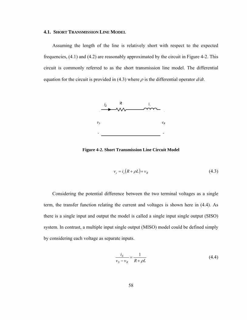
58
4.1. SHORT TRANSMISSION LINE MODEL
Assuming the length of the line is relatively short with respect to the expected
frequencies, (4.1) and (4.2) are reasonably approximated by the circuit in Figure 4-2. This
circuit is commonly referred to as the short transmission line model. The differential
equation for the circuit is provided in (4.3) where ρ is the differential operator d/dt.
Figure 4-2. Short Transmission Line Circuit Model
( ) Rss vLRiv ++= ρ (4.3)
Considering the potential difference between the two terminal voltages as a single
term, the transfer function relating the current and voltages is shown here in (4.4). As
there is a single input and output the model is called a single input single output (SISO)
system. In contrast, a multiple input single output (MISO) model could be defined simply
by considering each voltage as separate inputs.
LRvv
i
RS
S
ρ+=
−1 (4.4)

59
Because the proposed monitoring method uses sampled data, discrete-time models
are required. The bilinear transform (4.5) is used to approximate the continuous-time
behavior because it preserves model stability and does not exhibit aliasing in the
frequency response. The bilinear approximation can cause warping in the frequencies
close to the Nyquist frequency. However, as long as sufficient filtering is imposed and
sampling period, T, is small, the approximation of the continuous-time system should be
sufficiently accurate. Selecting y = is and u = vs-vr , the resulting difference equation is
shown in (4.6), where k is again used to indicate the current sample. In this case, the
output is selected to keep the transfer function from being improper, but this is not a
requirement for selecting the model’s form.
( )( )1
12+−
=zz
Ts (4.5)
( ) ( ) ( ) ( )1221
22−
+−
−−+
++
= kyLRTLRTku
LRTTku
LRTTky (4.6)
The three coefficients in (4.6) can be reduced by collecting the common parameter
terms as shown in (4.7). The new regressor vector is composed of two newly defined
terms (4.8) and is a function of both the input and output.
( ) ( ) ( )[ ] ( )1221
21
−+−
−−++
= kyLRTLRTkTukTu
LRTky (4.7)
( ) ( )
⎥⎦
⎤⎢⎣
⎡−−
−+=
)1(1
)(~ky
kTukTukTϕ (4.8)
60
In order to find a solution using linear regression techniques, the model must be
considered “linear in the parameters.” Linear in the parameters implies the unknown
coefficients are not functions of each other or raised to any power. Clearly, the
coefficients are not linear in terms of the R and L parameters but can be redefined or
reparameterized with respect to the parameters to be estimated. The reparameterized
model is given in (4.9) and (4.10).
LRTLRTD
LRTD
22
21
2
1
+−
=
+=
(4.9)
( ) ( ) ( )( )[ ] ( )[ ]11 21 −−+−+= kyDkukuDky (4.10)
There is a penalty for reparameterizing the model. Specifically, the physical
relationships designated in (4.9) between R and L are not enforced by the estimation
procedure. In other words, the parameters D1 and D2 are determined merely on how well
the curve fit of (4.10) models the observed input-output data. Nevertheless if the model is
a good physical representation of the line and a unique solution is found for the
parameters, the estimated parameters provide good approximations of the physics-based
parameters. That is, R and L can be approximated from the D1 and D2 using the
relationships given in (4.11). Reparameterization can lead to unidentifiable parameters if
a mapping does not exist between the estimated and physics-based parameters. In these
instances, diagnosis and prognosis measures could be based on the estimated coefficients.

61
1
2
1
2
141
121
DD
L
DD
TR
−⎟⎠⎞
⎜⎝⎛=
+⎟⎠⎞
⎜⎝⎛=
(4.11)
Reparameterization of this model can be avoided though a different selection of
which variable to model as the output as shown in (4.12) and (4.13). While this model
contains a derivative in the regressors, the numerical sensitivity to measurement errors is
not any better or worse than that associated with the reparameterization. Additionally,
models that permit the direct estimation of the physics-based parameters are intuitively
easier to analyze. In contrast, the variances of R and L using (4.11) are dependent on
nonlinear relationships between the variances of D1 and D2. When possible, direct
estimation of the physics-based parameters is preferred.
LRi
vvuy
S
RS ρ+=−
= (4.12)
( ) ( ) ( ) ( )[ ] ( )⎥⎦⎤
⎢⎣⎡ −−+−+=−+ )1()(*211 kukuT
LkukuRkyky (4.13)
4.2. NOMINAL PI CIRCUIT MODEL
A two-conductor line model is presented in Figure 4-3 with both conductors
retaining their individual resistance and inductance terms. Additionally, the model
includes the shunt capacitance (equally divided at the two ends of the line) as well as
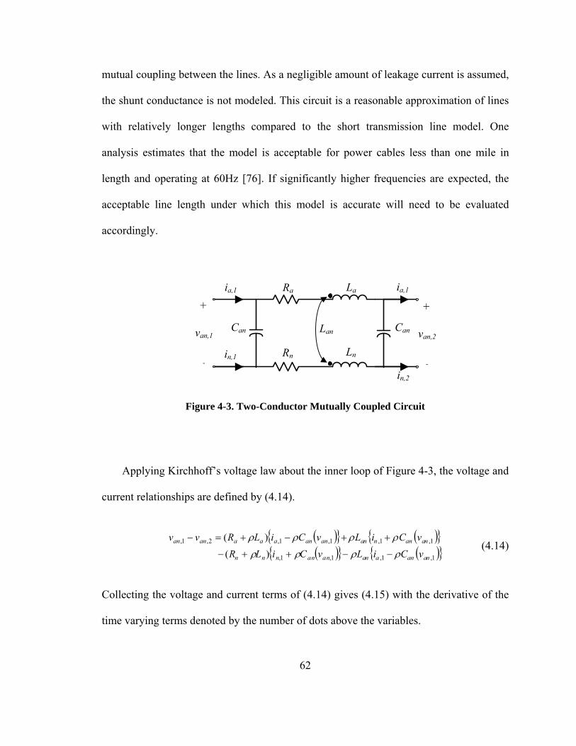
62
mutual coupling between the lines. As a negligible amount of leakage current is assumed,
the shunt conductance is not modeled. This circuit is a reasonable approximation of lines
with relatively longer lengths compared to the short transmission line model. One
analysis estimates that the model is acceptable for power cables less than one mile in
length and operating at 60Hz [76]. If significantly higher frequencies are expected, the
acceptable line length under which this model is accurate will need to be evaluated
accordingly.
ia,1 Ra La ia,1
Can
Rn Ln
Lan
in,1
in,2
+
van,1
-
Can
+
van,2
-
Figure 4-3. Two-Conductor Mutually Coupled Circuit
Applying Kirchhoff’s voltage law about the inner loop of Figure 4-3, the voltage and
current relationships are defined by (4.14).
( ){ } ( ){ }( ){ } ( ){ }1,1,1,1,
1,1,1,1,2,1,
)()(
naananananannn
naannnaananaaaanan
vCiLvCiLRvCiLvCiLRvv
ρρρρ
ρρρρ
−−++−
++−+=− (4.14)
Collecting the voltage and current terms of (4.14) gives (4.15) with the derivative of the
time varying terms denoted by the number of dots above the variables.

63
[ ] [ ] ( ) ( )
( ) ( ) ⎥⎦
⎤⎢⎣
⎡−−⎥
⎦
⎤⎢⎣
⎡−+
⎥⎦
⎤⎢⎣
⎡+−−+⎥
⎦
⎤⎢⎣
⎡+−−=−
••
•••
1,1,
1,1,1,1,2,1, 2
nannaana
naannaanannaannnaaanan
iLLiLL
vLLLCvRRCiRiRvv (4.15)
Assuming current injected into either conductor is equal in magnitude but opposite in
sign (i.e. 1,1, na ii −= ), equation (4.15) reduces to (4.16). As indicated in (4.16), the
resistance and inductances were lumped together in order to reduce the number of
unknowns. While the individual conductor parameters cannot be determined
independently, the overall health can still be gauged by estimating of the equivalent
parameters. More importantly, by reducing the number of unknown parameters the
required excitation is reduced accordingly. The reduced two-conductor model can now be
represented by the nominal pi equivalent circuit presented in Figure 4-4; the terminal
voltages and currents were renamed to reduce notation. This circuit could also be derived
from the distributed parameter model of (4.1) and (4.2).
( )[ ] ( ) ( )
( ) ⎥⎦
⎤⎢⎣
⎡−+−
⎥⎦
⎤⎢⎣
⎡+−⎥
⎦
⎤⎢⎣
⎡−+++=−
••
••
1,
1,1,1,2,1,
2
2
naLC
annaan
anRC
naanaL
annaaR
naanan
vLLLC
vRRCiLLLiRRvv
444 3444 21
443442144 344 2143421
(4.16)

64
Figure 4-4. Nominal Pi Equivalent Circuit
It is initially assumed that voltage and current measurements on either end of the line
are available. The vector matrix relationship between the currents and voltages in the
circuit are defined by matrix 3(4.17). As with the short transmission line model, any of the
currents or voltages can be considered as the output or dependent variable.
⎥⎦
⎤⎢⎣
⎡
⎥⎥⎥⎥
⎦
⎤
⎢⎢⎢⎢
⎣
⎡
−+
−+
+−+
+=⎥⎦
⎤⎢⎣
⎡
R
S
R
S
vv
CLRLR
LRC
LRii
ρρρ
ρρ
ρ11
11
(4.17)
4.2.1. SISO MODEL
A SISO model was generated by subtracting the two rows of 3(4.17) and treating the
resulting voltage difference and current summation as single measurements. As shown in
3(4.18), selection of these input-output relations results in the cancellation of the R and L
terms. The bilinear transform was again employed to derive the equivalent difference
equation presented in (4.20).

65
[ ] ( ) ( ) [ ]RsRSRSRS
RS vvCC
vC
vLR
vvLR
vvii +=+++−
−+−
=− ρρρρρ 11
(4.18)
Cvvii
uy
RS
RS ρ=+−
= (4.19)
( ) ( ) ( )( )⎥⎦⎤
⎢⎣⎡ −−=−+ 121)( kukuT
Ckyky (4.20)
Another SISO model can be examined by writing the equations as the difference
between the voltage terms (or sum of the currents) as shown in (4.21). While the R and L
parameters are contained in the model, evaluation of (4.21) indicates they cannot be
directly estimated.
22 ++
+=
+−
=ρρ
ρRCLC
LRiivv
uy
RS
RS (4.21)
Utilizing the same process used previously to derive the simplified regression model, the
regressor model for this SISO model is given in (4.22) and (4.23).
( )
( ) ( ) ( ){ }( ) ( ){ }
( ) ( ){ }
( ){ } ⎥⎥⎥⎥⎥⎥
⎦
⎤
⎢⎢⎢⎢⎢⎢
⎣
⎡
−−−−
−−−−−−
−+−+
⎥⎦⎤
⎢⎣⎡=
22*)2(4)1(82214
222*212*
1 2
2
kyTkyky
kykyTkukuT
kukukuT
RCLCLRkyααααα
(4.22)
2224 TRCLC ++=α (4.23)

66
In this model, five parameters must be estimated before the three physical quantities can
be approximated, but the consequences of the reparameterization are more severe than
just increasing the required excitation. That is to say, if the excitation is ever insufficient
to determine the third parameter (1/α) all the physics-based parameter approximations
will be inaccurate. Clearly, this interdependence is unacceptable. The limitations of this
model highlight the benefits of selecting a model that permits the physics-based
parameters to be directly estimated. Other input-output combinations were investigated
but with similar shortcomings.
4.2.2. MISO MODEL
While a MIMO model could be derived from 3(4.17), the resulting model would not
permit direct estimation of R or L. The transfer function relationships in (4.17) are
therefore examined as individual MISO models. One possible MISO model is presented
in (4.24) which defines relationship between the terminal voltages and sending end
current injection shown in Figure 4-4.
RSs vLR
vCLR
i ⎟⎟⎠
⎞⎜⎜⎝
⎛+−
+⎟⎟⎠
⎞⎜⎜⎝
⎛+
+=
ρρ
ρ11 (4.24)
Selecting y= vR, u1= vS, and u2= iS, the corresponding difference equation is expressed in
4(4.25). The regressors for the model, (4.26) through (4.29), are expressed in terms of the
input-output observations and the reparameterized coefficients are expressed in terms of
the physical parameters as shown in (4.30). The receiving end voltage was selected as the

67
dependent variable, as it provided the least amount of reparameterization of the estimated
coefficients. Reparameterization of the coefficients was unavoidable, however, and
results in a model requiring a minimum 4th order excitation. While the excitation
requirement appears large at first, other forms of the model can be shown to require no
less than 5th order excitation.
( ) ( ) ( ) ( ) ( ) ( )[ ] ( ) ( ) ( ) ( )[ ]TkkkkDDDD
kukukukykyky
43214321
111
*
212212
ϕϕϕϕ=
−−−−−−+−+ (4.25)
( ) ( ) ( ) ( )241841212121 −+−−= ku
Tku
Tku
Tkϕ (4.26)
( ) ( ) ( )222112 −−= ku
Tku
Tkϕ (4.27)
( ) ( ) ( ) ( )212 2223 −−−−−= kukukukϕ (4.28)
( ) ( ) ( )222224 −+−= ku
Tku
Tkϕ (4.29)
LDRDRCDLCD ==== 4321 (4.30)
The unavoidable reparameterization of the physics-based parameters is not without
repercussions. Most importantly, the physical relationships designated in 4(4.30) are not
enforced. As a result, the capacitance is unidentifiable. While a secondary calculation can
be performed to approximate C, the accuracy of the approximation depends on the
accuracy of the individual parameter estimates. Additionally, there are two potential

68
approximations of C each requiring separate statistical evaluation. Therefore, the
estimates for the RC and LC parameters were treated as the final results required by the
proposed monitoring method. Rewriting (4.17) so that the MISO models use the two
current measurements results in similar reparameterization issues except, in this case, the
resistance and inductance will be unidentifiable.
As the algebraic relationships between the estimated coefficients are known, not
enforcing these relationships could be viewed as not taking advantage of all the available
information. Constraints could possibly be introduced to enforce the known physical
relationships. However, the resulting constraints are nonlinear and would require a
nonlinear optimization method.
4.2.3. SISO/MISO MODEL
The number of parameters in 4(4.25) can be reduced further when voltage and current
measurements at both ends of the line are available. In these cases, 4(4.20) is used to first
update the estimate of C which is subsequently used in 4(4.25) to reduce the unknowns to
R and L. The updated MISO model is provided in (4.31) through 4(4.33) with the most
recent update of C shown in the regressors. Given its dependence, the MISO portion of
the model requires an accurate estimation of C. In most cases the actual shunt capacitance
is relatively small compared to other parameters. As long as the error variance associated
with the estimate of C is not too great, its influence on the other estimates should be
minimal. If the shunt capacitance is negligible, (4.31) can be shown to be equivalent to
the short transmission line model of (4.13).

69
( ) ( ) ( ) ( ) ( ) ( )[ ] ( ) ( )[ ]TkkLR
kukukukykyky
21
111
*
212212
ϕϕ=
−−−−−−+−+ (4.31)
( ) ( ) ( ) ( )
( ) ( ) ( )212
222*
222
111
−−−−−⎭⎬⎫
⎩⎨⎧ −−=
kukuku
kuT
kuT
kCkϕ (4.32)
( ) ( ) ( ) ( ) ( )
( ) ( )222
24184*
22
1212122
−+−
⎭⎬⎫
⎩⎨⎧ −+−−=
kuT
kuT
kuT
kuT
kuT
kCkϕ (4.33)
Not only does this two-tier method directly estimate the physics-based parameters, it
also reduces the minimum excitation to 2nd order. Therefore if both voltages and currents
are available, the parameters can be estimated given only the fundamental frequency.
However, when one of the currents is unavailable, the loss of information supplied from
the measurement must be offset by doubling the minimum required excitation.
4.2.4. SHUNT CONDUCTANCE
Shunt conductance can be included in the nominal pi circuit model if leakage
currents through the dielectric material are expected, or if it is a key measure of the
cable’s health. Inclusion of this parameter does not significantly influence the general
form of the models previously developed. However, it does introduce an additional
parameter which increases the excitation requirement in some models. For instance, the
SISO model difference equation is easily updated to include the shunt conductance as
70
shown in (4.34). Comparison with (4.20) shows that the only significant change is an
increase of the required persistence of excitation to 2nd order.
( ) ( ) ( )( )[ ] ( ) ( )( )⎥⎦⎤
⎢⎣⎡ −−+−+=−+ 1211)( kukuT
CkukuGkyky (4.34)
Similarly, the MISO model can be updated to include the shunt conductance.
However, this update does not alter the regressor portion of the model. Therefore,
equations (4.25) through (4.29) will remain the same. However, the redefined parameters
are now given by (4.35). Note that an accurate approximation of the shunt conductance
using this model not only relies on an accurate estimation of D2 but the accuracy of the
other three parameters as well.
LDRDGLRCDLCD ==+== 4321 (4.35)
4.3. MODEL EVALUATIONS In order to evaluate the estimation techniques and derived models, test data was
generated in PSPICE using the single-phase two bus system shown in Figure 4-5. The
nominal pi circuit model, connecting bus 1 and bus 2, represents one hundred feet of two
conductor 14-AWG cable characterized by R = 505 mΩ, L = 33.47 μH, and C = 0.895
pF. The load is represented by a constant impedance and the source is modeled by a 120
V 60 Hz voltage source with an internal impedance of 1 Ω. It should be noted that while
the fundamental frequency was chosen as 60 Hz, other fundamental frequencies would
provide the same order of excitation and therefore similar results. However, different

71
operating frequencies necessitate different sampling criteria and possibly model
structures.
Figure 4-5. Single-Phase Test Circuit
Gaussian white noise with variance σ 2 = 50x10-6 was introduced into the recorded
values to signify noise induced into the measurements before quantization. The values
were then quantized based on equivalent 16-bit data acquisition (DAQ) hardware set to
quantize the voltage and current on [-200, 200] V and [-20, 20] A ranges. While these
factors were chosen arbitrarily, changes to either are expected to influence the estimates
accordingly. It is recognized that steps to reduce both factors are key design criteria when
implementing the monitoring method.
Finally, before it is used by the solution algorithm, the measurement data is per-
unitized using the bases given in Table 4-1. The voltage, current, and time bases were
chosen to provide relatively uniform regressors values, while the parameter bases were
subsequently determined using the relationships defined in Table 3-2. While the voltage
base was selected to match the rated fundamental voltage, the current base is not as easily
selected given load variations. Therefore, a base of 10 A was heuristically selected to
emphasize the regressors associated with the resistance and inductance parameters of the

72
MISO model. The selection was made based on experience which indicated that during
low periods of excitation the R and L parameters show more signs of convergence than
the RC and LC estimates. Finally, the time base was selected to counter the radian
frequency scaling which occurs in the derivative terms. While the per-unit base values
were chosen based on the expected content in the fundamental frequency, varying
loading conditions, harmonics, and other system conditions will all influence the size of
the parameter space spanned by the regressors. Therefore, selection of the base values
must be done on an ad-hoc basis. Dynamic adjustments of the bases can be implemented
by the monitoring controller, but would require re-initializing the estimation algorithm.
Table 4-1. Test System Per-Unit Bases
Base Units Vbase 120 (V) Ibase 10 (A) tbase 2.653 (ms) Sbase 120 (VA) Rbase 120 (Ω) Lbase 318.3 (mH)Cbase 22.10 (μF)
In each of the following cases, the sampling period was fixed at T = 100 μs and a
forgetting factor of λ = 0.99 were specified in the MATLAB code implementing the
parameter estimation techniques. Additionally, the unknown parameter vector θ~ was set
to zero and the diagonals in P set to large values (1x10⁴) to indicate little confidence in
the initial values in θ~ . The SISO/MISO model combination was examined first to

73
illustrate the influence of measurement noise and λ. As the normal operation of the test
system was sufficient to meet the model’s excitation requirements, RLS with standard
exponential forgetting was used.
In order to evaluate the performance of the proposed method during abrupt changes
in the observations, a significant step change in the load was examined. The observed
voltage and current waveforms, during the load change, are illustrated in Figure 4-6. As
shown in Figure 4-7, the parameter estimates, using (4.20) and 4(4.31), quickly converge
to the true solutions, indicated by the dashed lines, but are not significantly influenced by
the load change. As the network change did not represent a change to the modeled
parameters, the extra excitation slightly improves the estimates.
Figure 4-6. Test Case Voltages and Currents
(a) Sending End and (b) Receiving End

74
Figure 4-7. SISO/MISO Model Parameter Estimates during
a Load Change.
As previously noted, parameter estimate accuracy is dependent on the measurement
noise. To illustrate the sensitivity, the test was performed again but with a 32-bit
quantization. The lower quantization error decreased the variance in each parameter
estimate as shown in Figure 4-8. However, the capacitance estimation is especially
sensitive to the noise given its dependence on the current differential between the line
terminals. This current is small by nature (as is the capacitance) which can be easily
overwhelmed by the noise contained in the two measurements. This is an inherent
difficulty when estimating the capacitance in general indicating the level of accuracy
required.

75
Figure 4-8. Parameter Estimates with 32-Bit Quantization
Error.
The sensitivity to measurement errors is also influenced by the equivalent memory
size determined by the forgetting factor. When the forgetting factor of the SISO model
was increased to 0.999, representing an order of magnitude increase to the equivalent
memory size, the variance was reduced significantly, as shown in Figure 4-9. As R and L
are estimated by a model with the original setting for λ, their potential tracking ability
was not altered but their variance was still reduced through their dependence on the
estimate of C.
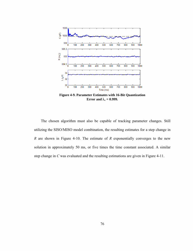
76
Figure 4-9. Parameter Estimates with 16-Bit Quantization
Error and λc = 0.999.
The chosen algorithm must also be capable of tracking parameter changes. Still
utilizing the SISO/MISO model combination, the resulting estimates for a step change in
R are shown in Figure 4-10. The estimate of R exponentially converges to the new
solution in approximately 50 ms, or five times the time constant associated. A similar
step change in C was evaluated and the resulting estimations are given in Figure 4-11.

77
Figure 4-10. Parameter Estimates for Step Change in R.
Figure 4-11. Parameter Estimates for Step Change in C.

78
Recursive parameter estimation using the MISO model is evaluated in the same
manner as with the SISO/MISO evaluations. The model contains four parameters which
increases the required excitation to a minimum 4th order. To stress the MISO model’s
increased identifiability requirements, the parameters were first estimated using RLS with
standard exponential forgetting and the same load change used before. The estimated
parameters are provided in Figure 4-12. Until the transient from the load change occurs,
the 60Hz signal alone does not provide sufficient excitation for convergence of the
estimates to occur. However during the transient, the excitation temporarily increases and
the solution converges to the true values. Nonetheless, after the transient decays the
exciting information is eventually discounted and the parameters drift from the converged
solution. Note that both the mean and variance of the parameter estimates are affected.
The loss of information was also indicated by the 95% confidence margins or error
shown in Figure 4-13. The values in Figure 4-13 represent the margin or error which
contains the true solution with confidence level of 95%. During the transient, the
confidence interval decreased significantly but increases once the information was
discounted. The principle factors in the changing confidence intervals were similar trends
in the covariance matrix diagonals. As P increased, the increased sensitivity to noise gave
rise to increased estimate variance as seen in Figure 4-12. Given the lack of constant
excitation in this scenario, some form of estimator windup prevention is clearly desirable.
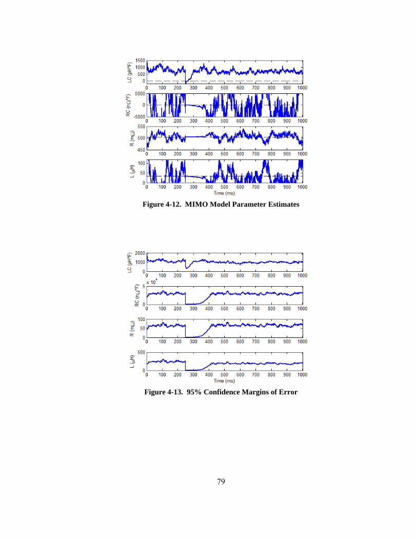
79
Figure 4-12. MIMO Model Parameter Estimates
Figure 4-13. 95% Confidence Margins of Error
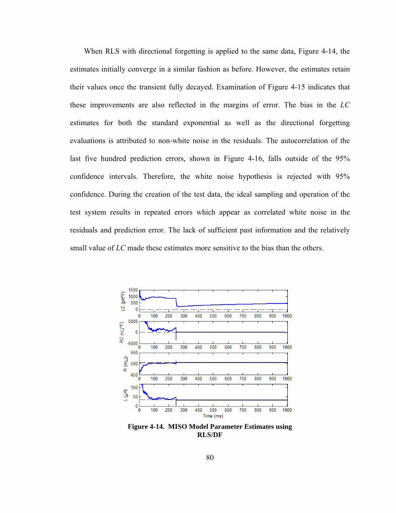
80
When RLS with directional forgetting is applied to the same data, Figure 4-14, the
estimates initially converge in a similar fashion as before. However, the estimates retain
their values once the transient fully decayed. Examination of Figure 4-15 indicates that
these improvements are also reflected in the margins of error. The bias in the LC
estimates for both the standard exponential as well as the directional forgetting
evaluations is attributed to non-white noise in the residuals. The autocorrelation of the
last five hundred prediction errors, shown in Figure 4-16, falls outside of the 95%
confidence intervals. Therefore, the white noise hypothesis is rejected with 95%
confidence. During the creation of the test data, the ideal sampling and operation of the
test system results in repeated errors which appear as correlated white noise in the
residuals and prediction error. The lack of sufficient past information and the relatively
small value of LC made these estimates more sensitive to the bias than the others.
Figure 4-14. MISO Model Parameter Estimates using
RLS/DF

81
Figure 4-15. 95% Confidence Margins of Error
Figure 4-16. Prediction Error Autocorrelation

82
The information contained in the switching transient increases the excitation of the
dynamics well beyond the 4th order excitation required by the MISO model. In order to
show that accurate parameter estimates can be made given the minimum required
excitation, the next example used a 5th harmonic current injection to temporarily increase
the excitation to 4th order. The harmonic is injected at the load starting at 250 ms and for
a period of 500 ms. No other system or load changes occur during this time. Voltage and
current waveforms before and after the start of the harmonic injection are shown in
Figure 4-17 to illustrate the change in the measured waveforms. As shown in Figure 4-18,
the RLS solution quickly converged during the harmonic injection due to the increased
excitation. However, the estimates again drift once the additional excitation is removed.
In contrast, the RLS with directional forgetting shows no signs of drifting estimates as
seen in Figure 4-19. It is also interesting to note that information observed during the
harmonic injection results in the estimate of LC being less sensitive to bias than in Figure
4-14.
Figure 4-17. Sending End Voltage and Current Waveforms
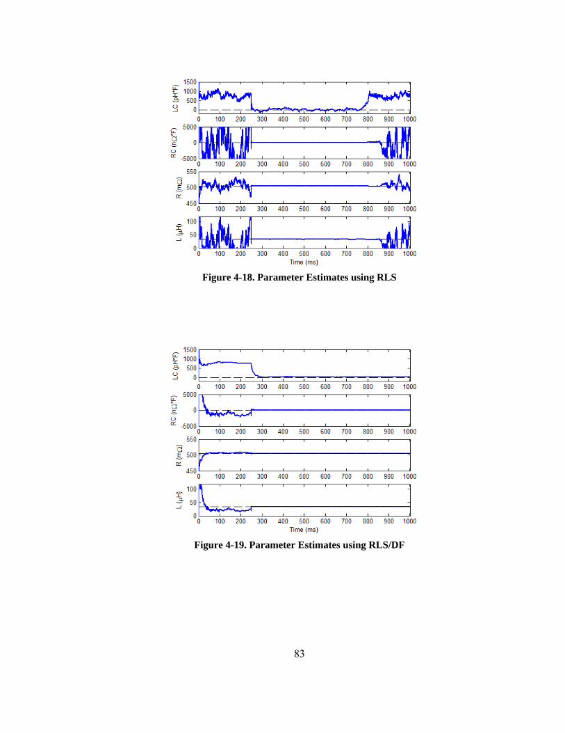
83
Figure 4-18. Parameter Estimates using RLS
Figure 4-19. Parameter Estimates using RLS/DF
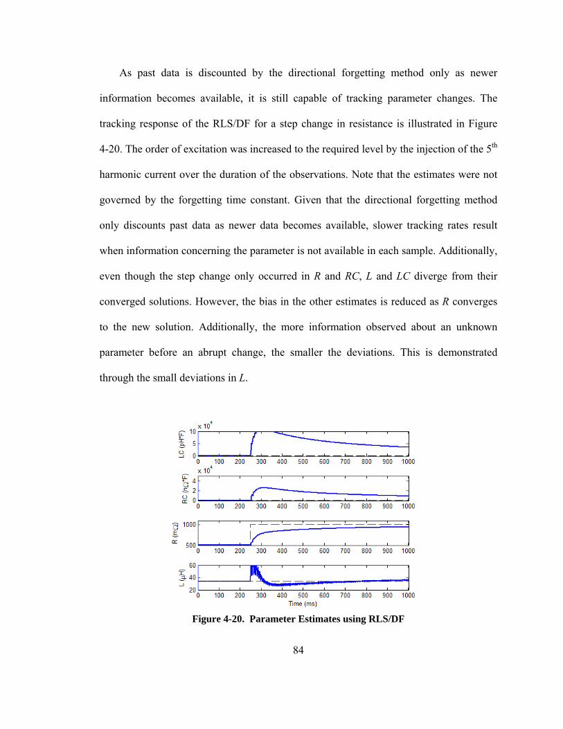
84
As past data is discounted by the directional forgetting method only as newer
information becomes available, it is still capable of tracking parameter changes. The
tracking response of the RLS/DF for a step change in resistance is illustrated in Figure
4-20. The order of excitation was increased to the required level by the injection of the 5th
harmonic current over the duration of the observations. Note that the estimates were not
governed by the forgetting time constant. Given that the directional forgetting method
only discounts past data as newer data becomes available, slower tracking rates result
when information concerning the parameter is not available in each sample. Additionally,
even though the step change only occurred in R and RC, L and LC diverge from their
converged solutions. However, the bias in the other estimates is reduced as R converges
to the new solution. Additionally, the more information observed about an unknown
parameter before an abrupt change, the smaller the deviations. This is demonstrated
through the small deviations in L.
Figure 4-20. Parameter Estimates using RLS/DF

85
The parameter estimates using RLS with standard forgetting for the same dataset is
provided in Figure 4-21. Note that similar deviations in the parameters estimated
occurred using this method as well. Obviously, tracking the parameter changes using
directional forgetting takes considerably longer when compared to the standard method
of discounting. Nevertheless, in situations where the excitation is intermittent in nature
the prevention of parameter drift greatly outweighs a faster tracking ability. Still, for
certain applications it may be sufficient to estimate the parameters with RLS and then
only retain estimates whose margins of error satisfy predetermined tolerances.
Figure 4-21. Parameter Estimates using RLS
The tracking response of the directional forgetting method to the abrupt change
might be improved by varying λ in response to the prediction error. The results when
variable directional forgetting, as discussed in section 3.2.2, was applied to the dataset are

86
shown in Figure 4-22. As λ is no longer constant it is also provided in Figure 4-22. As
shown, dynamically altering the memory size allowed the solution to more quickly track
the parameter changes. Notice the variance of L is also significantly larger than in Figure
4-20 due to the increased discounting of information relevant to this parameter.
Figure 4-22. Parameter Estimates using RLS/VDF
Model selection should consider many factors such as the necessary parameters for
accurate condition monitoring and the expected parameter magnitudes relative to the
noise levels and/or measurement accuracy. The capacitance associated with short spans
of wire is particularly difficult to estimate due to its relatively small value. This was seen

87
not only in the SISO/MISO model combination, but also in the MISO results which
indicate the estimates of RC and LC are far from ideal.
If the estimation of a particular parameter is unnecessary, or unfeasible, one option is
to reduce the model order by discarding the parameter. Removing the variable from the
model not only reduces the required level of excitation but also reduces variance in the
parameter estimates due to parsimony. On the other hand, this does not mean that just any
parameter can be removed from the model without consequence. In fact, any unmodeled
content will end up in the residuals of the least-squares solution violating the assumption
that the residuals consist of white noise. The non-white signals in the residuals will in
turn result in biased parameter estimates as well as inaccurate variance estimates.
Multiple models could be estimated in parallel if different models are expected to
offer better estimations during varying conditions. A comparison of the 95% confidence
intervals for three model types is given in Table 4-2; the SISO/MISO model combination,
the MISO model alone, and the short transmission line model (RL). Each model’s
parameters were estimated using one second of data containing the fundamental and 5th
harmonic waveforms. While the results in Table 4-2 are not meant to be statistically
conclusive, the results do support earlier conclusions. For example, the SISO model
(which has the benefit of the additional information from the 2nd current measurement)
provides the most accurate means to estimate the capacitance. Obviously the wide
variances associated with the estimates of RC and LC will result in a low level of
confidence if either is used to approximate C. Moreover, the confidence intervals for both
RC and LC cross zero which indicates that these parameters can potentially be removed

88
from the model. Another interpretation would be that the margin of error is larger than
the estimate itself. Actually, the margins of error for these parameters are nearly twice the
estimates. Consequently, very little if any bias is present when the capacitance terms are
removed as seen by the results for the short transmission line model (RL) model.
However, the estimates of RC and LC are not without merit as the capacitance could
increase over time to a level where its dynamic contributions were no longer negligible.
If this were the case, it would be very important to have the capacitance modeled as not
to introduce bias into the estimations. Including the capacitance did not show signs of
significantly increasing the other parameter variances.
Table 4-2. 95% Univariate Confidence Intervals
R (mΩ) L (μH) C (nF) RC (nΩF) LC (pHF)
Low High Low High Low High Low High Low High
SISO/MISO 504.99 505.01 33.47 33.48 0.790 1.085 NA NA NA NA
MISO 504.90 505.00 33.42 33.59 NA NA -5.983 13.320 -11.84 39.32
RL 504.94 505.03 33.40 33.63 NA NA NA NA NA NA
The techniques are also applicable to DC networks. While constant DC values only
provide a 1st order excitation, i.e. sufficient excitation to estimate the line resistance,
transient events increase the excitation to sufficient levels to estimate other model
parameters. If we assume that these events will not occur with any predictable regularity,
directional forgetting should provide better estimates than standard directional forgetting.
In order to examine how well the directional forgetting algorithm handles periods of low

89
excitation between short bursts of high excitation, a case consisting of a periodically
switched RL load connected to a 24 V DC system is evaluated. The observed voltage and
currents at both ends of the line are presented in Figure 4-23 and the same example line
of the previous simulations is assumed to connect the load to the 24 V source. During the
estimations, base values of Vbase = 24 V, Ibase = 10 A, and Tbase = 10 μs were used to
normalize the measurements. The values were again heuristically chosen in an attempt to
provide regressors whose magnitudes would be within the same general range.
Figure 4-23. DC Signals for a Switching DC Load
(a) Sending End and (b) Receiving End
For this example, the sampling period was increased to 10 μs in order to better
observe the faster dynamics of the transient while the forgetting factor was left at λ =
0.99. While the switching transients increase the excitation, they also contain frequencies

90
higher than the Nyquist frequency. For that reason, anti-aliasing filters were introduced
during the generation of the test data. Identical second order low-pass filters with 5 kHz
cutoff frequencies were used as the anti-aliasing filters for each measurement. The high
sampling frequency also results in five thousand samples being observed between each
switching transient. Even though the transients occur at fixed intervals, the resulting
excitation can still be considered intermittent in nature.
The parameter estimations for the short transmission line model using the RLS/DF
algorithm are given in Figure 4-24. As expected, during the steady-state periods only
information concerning the resistance is available and this parameter quickly converges
to its “true” value. However, during the transient periods the dynamics associated with
the inductor are excited and the estimate begins to approach a converged solution. While
the switching transients in the example are equally spaced this is not a requirement as the
directional forgetting algorithm clearly shows no signs of estimate drift during the low
excitation periods.
In contrast, the solution using standard discounting, as shown in Figure 4-25, clearly
drifts during each period of low excitation. The estimates using directional forgetting also
show indications of improving over time. This improvement can be attributed to the
retention of the relevant information during each event whereas the standard method
steadily discounts information as time progresses. For instance, based on the time
constant approximation of (3.35) and the selected forgetting factor, the information
gained during the transient is completely discounted after 500 samples. Given that there
is an order of magnitude more samples between the transients, there is ample time for the
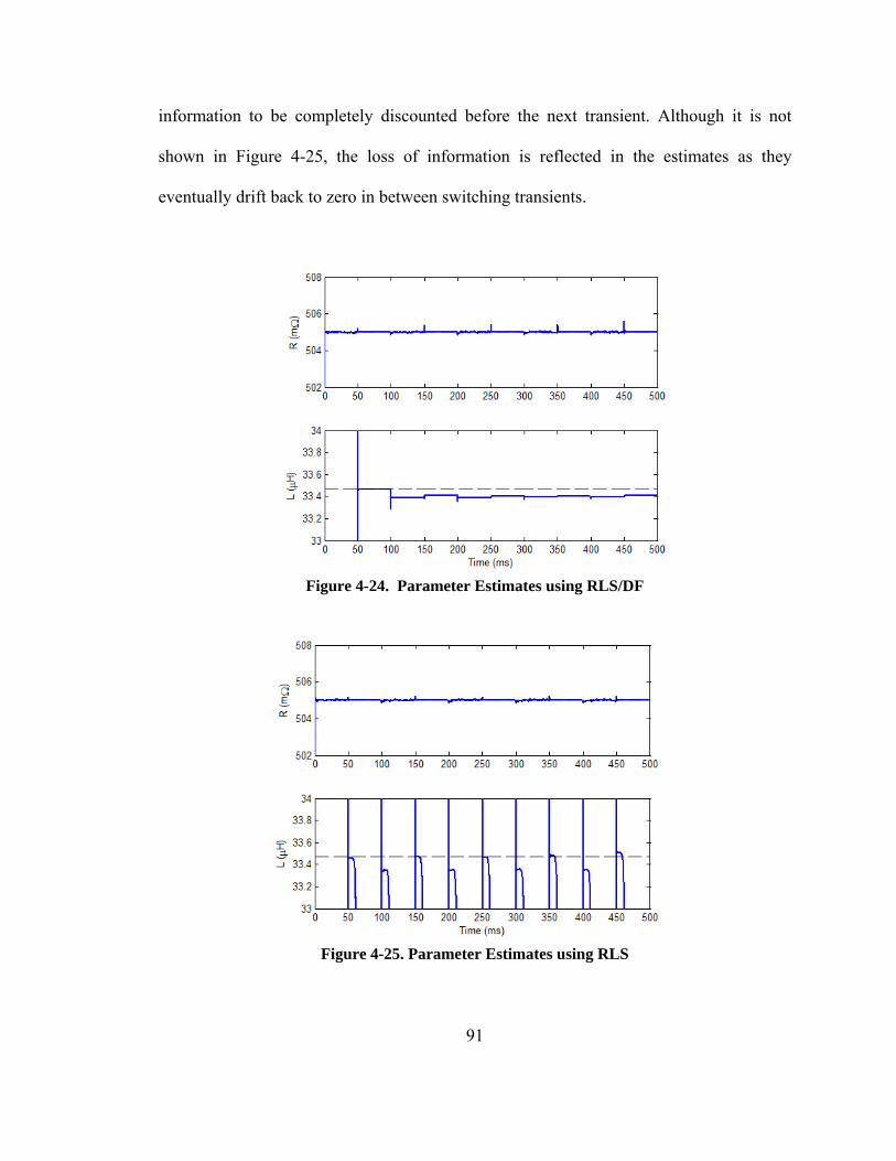
91
information to be completely discounted before the next transient. Although it is not
shown in Figure 4-25, the loss of information is reflected in the estimates as they
eventually drift back to zero in between switching transients.
Figure 4-24. Parameter Estimates using RLS/DF
Figure 4-25. Parameter Estimates using RLS

92
4.4. SUMMARY
In cases where the excitation is intermittently sufficient, directional forgetting is
clearly a better alternative to standard exponential discounting. The method has been
shown to provide accurate solutions of two-conductor wiring physical-based parameters
under intermittent conditions while retaining the ability to track parameter changes.
Accuracy of the physically-based parameter estimates was also shown to be dependent
upon the measurement type, measurement noise, as well as the model formulation. The
level of accuracy was gauged by recursively calculated margins of error which are not
only easily calculated but necessary to interface the estimates with stochastic prognosis
techniques. The same techniques as applied to multiple conductor models are examined
in the next chapter. While the multiple conductor models are innately more complex, the
conclusions derived in this chapter concerning the effectiveness of the parameter
estimation techniques still hold true.
93
CHAPTER 5
MULTIPLE CONDUCTOR MODELS
In this chapter the identifiability requirements of multiple conductor network
elements are examined. The presented models are based on general assumptions
concerning conductor characteristics and the availability of time-domain measurements.
Due to the additional interactions that exist between conductors in close proximity, the
models and identifiability requirements in this chapter represent an increased complexity
compared to the models of the previous chapter. The identifiability requirements are
examined under the assumption of intermittent excitation, as the identifiability
requirements are intended to facilitate the monitoring method described in Chapter 1.
Lines with more than two conductors can be approached in a similar fashion as two-
conductor lines except for the obvious increase to the number of required measurements
and unknown parameters. A multiple conductor model including mutual coupling and
capacitance between conductors 1 through n is shown in Figure 5-1. It is assumed that the
nth conductor models the return path, whether it is a neutral conductor, shield, vehicle
hull, or combination of the three. Given voltage measurements at both ends of the
conductors and currents at only one side, the relationships between the measured values
and the unknown parameters values can be described by (5.1) and (5.2). In the matrix of

94
(5.1) the diagonals represent the total capacitance connected to the node (i.e., C11 =
C12+C1n+..., C22 = C12+C2n+..., etc.). However, measurement using the equipotential
reference depicted in Figure 5-1 is not practical in many applications. It is also beneficial
to reduce the number of unknown parameters by lumping the neutral’s parameters in with
the other conductors.
⎥⎥⎥⎥⎥
⎦
⎤
⎢⎢⎢⎢⎢
⎣
⎡
⎥⎥⎥⎥
⎦
⎤
⎢⎢⎢⎢
⎣
⎡
−−
−−−−
−
⎥⎥⎥⎥⎥
⎦
⎤
⎢⎢⎢⎢⎢
⎣
⎡
=
⎥⎥⎥⎥⎥
⎦
⎤
⎢⎢⎢⎢⎢
⎣
⎡
1,
1,2
1,1
21
22212
11211
1,
1,2
1,1
*
*2
*1
nnnnn
n
n
nnv
vv
dtd
CCC
CCCCCC
i
ii
i
ii
MOM
L
MM (5.1)
⎥⎥⎥⎥⎥
⎦
⎤
⎢⎢⎢⎢⎢
⎣
⎡
⎥⎥⎥⎥
⎦
⎤
⎢⎢⎢⎢
⎣
⎡
+
⎥⎥⎥⎥⎥
⎦
⎤
⎢⎢⎢⎢⎢
⎣
⎡
⎥⎥⎥⎥
⎦
⎤
⎢⎢⎢⎢
⎣
⎡
=
⎥⎥⎥⎥⎥
⎦
⎤
⎢⎢⎢⎢⎢
⎣
⎡
−
−−
*
*2
*1
21
22212
11211
*
*2
*1
22
11
2,1,
2,21,2
2,11,1
nnnnn
n
n
nnnnn i
ii
dtd
LLL
LLLLLL
i
ii
R
RR
vv
vvvv
M
L
MOM
L
MOM (5.2)
L12
L11
L1n
R11
R22
L2n
L22
LnnRnn
C12
C1nC2n
2
n
i1*v1,11
v2,1
vn,1
v1,2
v2,2
vn,2
C12
C2nC1n
i2*
in*
i1,1
i2,1
in,1
Figure 5-1. Multiple Conductor Line Model

95
By subtracting the last equation in (5.2) from the rest of the rows, the voltages are
redefined as between the individual phases and the neutral, as shown in (5.3), eliminating
the need for the equipotential plane shown in Figure 5-1.
⎥⎥⎥⎥⎥
⎦
⎤
⎢⎢⎢⎢⎢
⎣
⎡
⎥⎥⎥⎥
⎦
⎤
⎢⎢⎢⎢
⎣
⎡−−−−−−
+
⎥⎥⎥⎥⎥
⎦
⎤
⎢⎢⎢⎢⎢
⎣
⎡
⎥⎥⎥⎥
⎦
⎤
⎢⎢⎢⎢
⎣
⎡−−
=
⎥⎥⎥⎥
⎦
⎤
⎢⎢⎢⎢
⎣
⎡−−
*
*2
*1
2222112
1212111
*
*2
*1
22
11
2,21,2
2,11,1
0000000 n
nnnnn
nnnnn
n
nn
nn
nn
nn
i
ii
dtdLLLLLL
LLLLLL
i
ii
RRRR
vvvv
M
L
MOM
L
M
L
MOM(5.3)
Kirchhoff’s current law states that at every instant in time the sum of the currents across
any cut-set equals zero. Hence, the currents (and their derivatives) sum to zero and the
bottom row of (5.4) can be set to one.
⎥⎥⎥⎥⎥
⎦
⎤
⎢⎢⎢⎢⎢
⎣
⎡
⎥⎥⎥⎥
⎦
⎤
⎢⎢⎢⎢
⎣
⎡−−−−−−
+
⎥⎥⎥⎥⎥
⎦
⎤
⎢⎢⎢⎢⎢
⎣
⎡
⎥⎥⎥⎥
⎦
⎤
⎢⎢⎢⎢
⎣
⎡−−
=
⎥⎥⎥⎥
⎦
⎤
⎢⎢⎢⎢
⎣
⎡−−
*
*2
*1
2222112
1212111
*
*2
*1
22
11
2,21,2
2,11,1
1111110 n
nnnnn
nnnnn
n
nn
nn
nn
nn
i
ii
dtdLLLLLL
LLLLLL
i
ii
RRRR
vvvv
M
L
MOM
L
M
L
MOM (5.4)
Finally, through matrix and vector manipulations, it can be shown that (5.4) reduces to
(5.5).
⎥⎥⎥⎥⎥
⎦
⎤
⎢⎢⎢⎢⎢
⎣
⎡
⎥⎥⎥⎥
⎦
⎤
⎢⎢⎢⎢
⎣
⎡
−+−−+−−+
−−+−+−−+−−+−−+−+
+
⎥⎥⎥⎥⎥
⎦
⎤
⎢⎢⎢⎢⎢
⎣
⎡
⎥⎥⎥⎥
⎦
⎤
⎢⎢⎢⎢
⎣
⎡
+
++
=
⎥⎥⎥⎥⎥
⎦
⎤
⎢⎢⎢⎢⎢
⎣
⎡
−
−−
*
*2
*1
2211
222222112
112112111
*
*2
*1
22
11
2,1,
2,21,2
2,11,1
2
22
NNnnnNNNnnnnNNnnnnN
NnnnnNnnnnnnn
NnnnnNnnnnnnn
NnnNNnnnn
nnnnnn
nnnnnn
NnNn
nn
nn
i
ii
dtd
LLLLLLLLLLL
LLLLLLLLLLLLLLLLLLLLLL
i
ii
RRRR
RRRRRRRR
vv
vvvv
M
L
MOMM
L
M
L
MOM
L
M
(5.5)
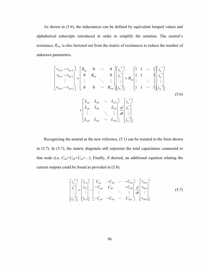
96
As shown in (5.6), the inductances can be defined by equivalent lumped values and
alphabetical subscripts introduced in order to simplify the notation. The neutral’s
resistance, Rnn, is also factored out from the matrix of resistances to reduce the number of
unknown parameters.
⎥⎥⎥⎥⎥
⎦
⎤
⎢⎢⎢⎢⎢
⎣
⎡
⎥⎥⎥⎥
⎦
⎤
⎢⎢⎢⎢
⎣
⎡
+
⎥⎥⎥⎥⎥
⎦
⎤
⎢⎢⎢⎢⎢
⎣
⎡
⎥⎥⎥⎥
⎦
⎤
⎢⎢⎢⎢
⎣
⎡
+
⎥⎥⎥⎥⎥
⎦
⎤
⎢⎢⎢⎢⎢
⎣
⎡
⎥⎥⎥⎥
⎦
⎤
⎢⎢⎢⎢
⎣
⎡
=
⎥⎥⎥⎥
⎦
⎤
⎢⎢⎢⎢
⎣
⎡
−
−−
*
*
*
*
*
*
*
*
*
2,1,
2,1,
2,1,
111
111111
00
0000
N
b
a
NNbNaN
bNbbab
aNabaa
N
b
a
nn
N
b
a
NN
bb
aa
NnNn
bnbn
anan
i
ii
dtd
LLL
LLLLLL
i
ii
R
i
ii
R
RR
vv
vvvv
M
L
MOM
L
M
L
MOM
L
M
L
MOM
L
M
(5.6)
Recognizing the neutral as the new reference, (5.1) can be restated in the form shown
in (5.7). In (5.7), the matrix diagonals still represent the total capacitance connected to
that node (i.e. Caa=Cab+Can+...). Finally, if desired, an additional equation relating the
current outputs could be found as provided in (5.8).
⎥⎥⎥⎥⎥
⎦
⎤
⎢⎢⎢⎢⎢
⎣
⎡
⎥⎥⎥⎥
⎦
⎤
⎢⎢⎢⎢
⎣
⎡
−−
−−−−
−
⎥⎥⎥⎥⎥
⎦
⎤
⎢⎢⎢⎢⎢
⎣
⎡
=
⎥⎥⎥⎥⎥
⎦
⎤
⎢⎢⎢⎢⎢
⎣
⎡
1,
1,
1,
1,
1,
1,
*
*
*
Nn
bn
an
NNbNaN
bNbbab
aNabaa
N
b
a
N
b
a
v
vv
dtd
CCC
CCCCCC
i
ii
i
ii
M
L
MOM
L
MM (5.7)

97
⎥⎥⎥⎥⎥
⎦
⎤
⎢⎢⎢⎢⎢
⎣
⎡
⎥⎥⎥⎥
⎦
⎤
⎢⎢⎢⎢
⎣
⎡
−−
−−−−
−
⎥⎥⎥⎥⎥
⎦
⎤
⎢⎢⎢⎢⎢
⎣
⎡
=
⎥⎥⎥⎥⎥
⎦
⎤
⎢⎢⎢⎢⎢
⎣
⎡
2,
2,
2,
*
*
*
2,
2,
2,
Nn
bn
an
NNbNaN
bNbbab
aNabaa
N
b
a
N
b
a
v
vv
dtd
CCC
CCCCCC
i
ii
i
ii
M
L
MOM
L
MM (5.8)
Substituting (5.7) into (5.6) and collecting like regressors, the linear regression model for
the multiple conductor line can be written as (5.9).
⎥⎥⎥⎥
⎦
⎤
⎢⎢⎢⎢
⎣
⎡
⎥⎥⎥⎥
⎦
⎤
⎢⎢⎢⎢
⎣
⎡
−
−−
⎥⎥⎥⎥
⎦
⎤
⎢⎢⎢⎢
⎣
⎡
+
⎥⎥⎥⎥
⎦
⎤
⎢⎢⎢⎢
⎣
⎡
⎥⎥⎥⎥
⎦
⎤
⎢⎢⎢⎢
⎣
⎡
−
−−
⎥⎥⎥⎥
⎦
⎤
⎢⎢⎢⎢
⎣
⎡
+
++
+
⎥⎥⎥⎥
⎦
⎤
⎢⎢⎢⎢
⎣
⎡
⎥⎥⎥⎥
⎦
⎤
⎢⎢⎢⎢
⎣
⎡
+
⎥⎥⎥⎥
⎦
⎤
⎢⎢⎢⎢
⎣
⎡
⎥⎥⎥⎥
⎦
⎤
⎢⎢⎢⎢
⎣
⎡
+
⎥⎥⎥⎥
⎦
⎤
⎢⎢⎢⎢
⎣
⎡
⎥⎥⎥⎥
⎦
⎤
⎢⎢⎢⎢
⎣
⎡
=
⎥⎥⎥⎥
⎦
⎤
⎢⎢⎢⎢
⎣
⎡
−
−−
1,
1,
1,
2
2
1,
1,
1,
1,
1,
1,
1,
1,
1,
1,
1,
1,
2,1,
2,1,
2,1,
111
111111
00
0000
Nn
bn
an
NNbNaN
bNbbab
aNabaa
NNbNaN
bNbbab
aNabaa
Nn
bn
an
NNbNaN
bNbbab
aNabaa
nnNNnnnn
nnnnbbnn
nnnnnnaa
N
b
a
NNbNaN
bNbbab
aNabaa
N
b
a
nn
N
b
a
NN
bb
aa
NnNn
bnbn
anan
v
vv
dtd
CCC
CCCCCC
LLL
LLLLLL
v
vv
dtd
CCC
CCCCCC
RRRR
RRRRRRRR
i
ii
dtd
LLL
LLLLLL
i
ii
R
i
ii
R
RR
vv
vvvv
M
L
MOM
L
L
MOM
L
M
L
MOM
L
L
MOM
L
M
L
MOM
L
M
L
MOM
L
M
L
MOM
L
M
(5.9)
As the number of conductors increase, so do the number of unknowns in each model.
However, it can be shown that when modeling N>2 conductors, equation (5.9) requires N
less parameters than the line model of Figure 5-1.
The equivalent model for a four conductor cable is provided in Figure 5-2.
Examining the equations individually, as done during the two-conductor model analyses,
each phase can be evaluated using individual MISO models. Note that the individual
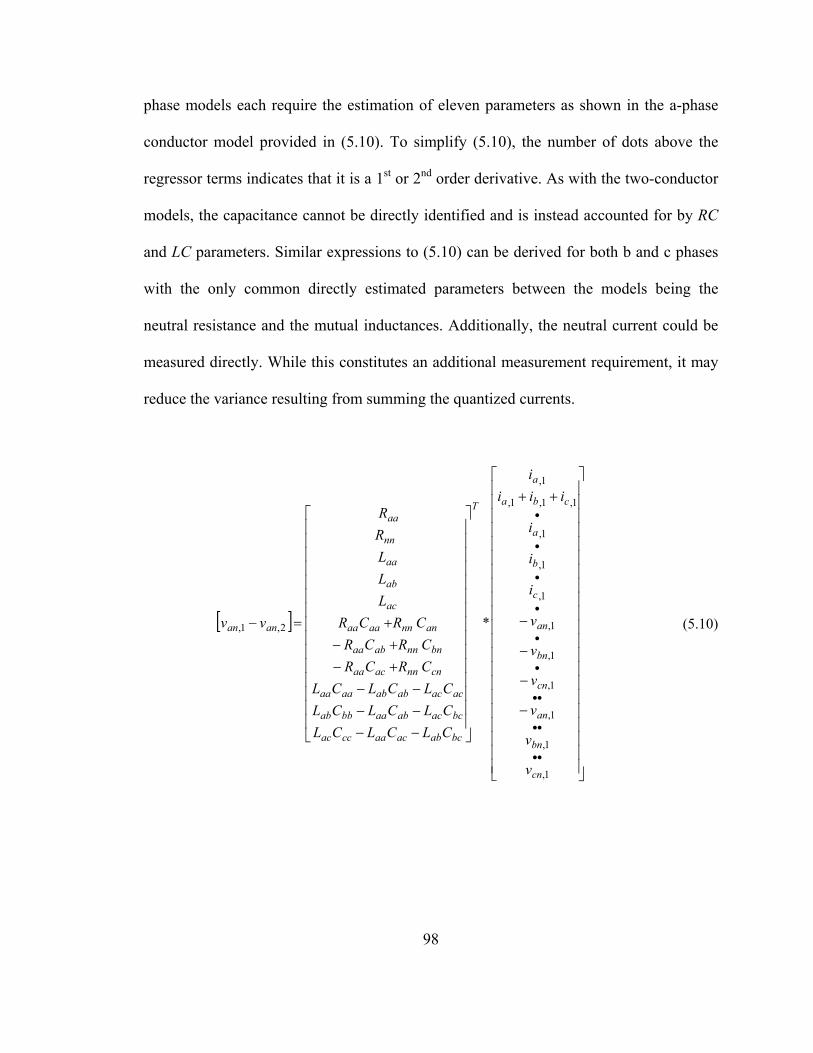
98
phase models each require the estimation of eleven parameters as shown in the a-phase
conductor model provided in (5.10). To simplify (5.10), the number of dots above the
regressor terms indicates that it is a 1st or 2nd order derivative. As with the two-conductor
models, the capacitance cannot be directly identified and is instead accounted for by RC
and LC parameters. Similar expressions to (5.10) can be derived for both b and c phases
with the only common directly estimated parameters between the models being the
neutral resistance and the mutual inductances. Additionally, the neutral current could be
measured directly. While this constitutes an additional measurement requirement, it may
reduce the variance resulting from summing the quantized currents.
[ ]
⎥⎥⎥⎥⎥⎥⎥⎥⎥⎥⎥⎥⎥⎥⎥⎥⎥⎥⎥⎥⎥
⎦
⎤
⎢⎢⎢⎢⎢⎢⎢⎢⎢⎢⎢⎢⎢⎢⎢⎢⎢⎢⎢⎢⎢
⎣
⎡
−
−
−
−
++
⎥⎥⎥⎥⎥⎥⎥⎥⎥⎥⎥⎥⎥⎥⎥
⎦
⎤
⎢⎢⎢⎢⎢⎢⎢⎢⎢⎢⎢⎢⎢⎢⎢
⎣
⎡
−−−−−−
+−+−
+=−
••
••
••
•
•
•
•
•
•
1,
1,
1,
1,
1,
1,
1,
1,
1,
1,1,1,
1,
2,1, *
cn
bn
an
cn
bn
an
c
b
a
cba
a
T
bcabacaaccac
bcacabaabbab
acacababaaaa
cnnnacaa
bnnnabaa
annnaaaa
ac
ab
aa
nn
aa
anan
v
v
v
v
v
v
i
i
i
iiii
CLCLCLCLCLCLCLCLCL
CRCRCRCR
CRCRLLLRR
vv (5.10)

99
Figu
re 5
-2. F
our-
Con
ucto
r L
ine
Mod
el

100
Numerous other model configurations can be derived based on various conductor
configurations and characteristic assumptions. If the mutual coupling is assumed to be
equal in each phase, the unknowns can be reduced by modeling the mutual coupling by a
single term, Lm. Additionally, given current and voltage measurements at both ends of the
conductors, the capacitances could be determined independently of the resistance and
inductance terms as indicated by the three-phase model shown in (5.11). Equation (5.11)
was derived using the relationships in (5.7) and (5.8).
⎥⎥⎥
⎦
⎤
⎢⎢⎢
⎣
⎡
+++
⎥⎥⎥
⎦
⎤
⎢⎢⎢
⎣
⎡
−−−−−−
=⎥⎥⎥
⎦
⎤
⎢⎢⎢
⎣
⎡
−−−
2,1,
2,1,
2,1,
2,1,
2,1,
2,1,
cncn
bnbn
anan
ccbcac
bcbbab
acabaa
cc
bb
aa
vvvvvv
dtd
CCCCCCCCC
iiiiii
(5.11)
While the multi-conductor models are considerably more complex, the estimation
algorithms remain unchanged. The same generalized conclusions concerning
convergence, estimator drift, and parameter tracking equally apply to the multi-conductor
models as to the two-conductor models. However, interactions between the conductors
results in linearly dependent regressors for most system conditions. Hence, identification
of the modeled parameters requires more than sufficient harmonic content. It should also
be noted that additional models could be produced as long as the derived models are
linear.
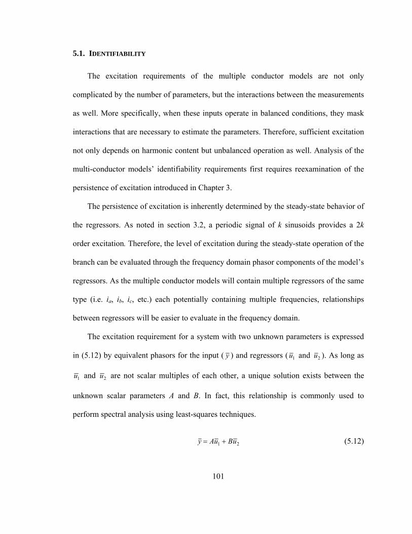
101
5.1. IDENTIFIABILITY
The excitation requirements of the multiple conductor models are not only
complicated by the number of parameters, but the interactions between the measurements
as well. More specifically, when these inputs operate in balanced conditions, they mask
interactions that are necessary to estimate the parameters. Therefore, sufficient excitation
not only depends on harmonic content but unbalanced operation as well. Analysis of the
multi-conductor models’ identifiability requirements first requires reexamination of the
persistence of excitation introduced in Chapter 3.
The persistence of excitation is inherently determined by the steady-state behavior of
the regressors. As noted in section 3.2, a periodic signal of k sinusoids provides a 2k
order excitation. Therefore, the level of excitation during the steady-state operation of the
branch can be evaluated through the frequency domain phasor components of the model’s
regressors. As the multiple conductor models will contain multiple regressors of the same
type (i.e. ia, ib, ic, etc.) each potentially containing multiple frequencies, relationships
between regressors will be easier to evaluate in the frequency domain.
The excitation requirement for a system with two unknown parameters is expressed
in (5.12) by equivalent phasors for the input ( y ) and regressors ( 1u and 2u ). As long as
1u and 2u are not scalar multiples of each other, a unique solution exists between the
unknown scalar parameters A and B. In fact, this relationship is commonly used to
perform spectral analysis using least-squares techniques.
21 uBuAy += (5.12)

102
Multi-phase power systems are typically operated as near to balanced conditions as
possible. However, balanced operation actually limits the excitation in the measurements.
Consider the estimation of three unknowns using three phasor measurements, 1u , 2u , and
3u . If only a single frequency is considered, only two equations – the real and imaginary
portions of (5.13) – can be written relating these three parameters. As an infinite number
of regressor vector combinations will provide the predicted output vector, a unique
solution cannot be determined.
321 uCuBuAy ++= (5.13)
If an additional sinusoid is included, the number of equations appears to increase to a
sufficient level as indicated in (5.14).
αωαωαωαω
ωωωω
,uC,uB,uAy,uC,uB,uAy
321
321
++=++=
(5.14)
However, if the phasors are related through a scalar, as shown in (5.15), the number of
effective equations reduces to two.
⎥⎥⎥⎥
⎦
⎤
⎢⎢⎢⎢
⎣
⎡
=
⎥⎥⎥⎥
⎦
⎤
⎢⎢⎢⎢
⎣
⎡
αω
αω
αω
αω
ω
ω
ω
ω
,u,u,u
y
x*
,u,u,u
y
3
2
1
3
2
1 (5.15)
Consequently, balanced operation will always limit the persistence of excitation to 2nd
order regardless of the number of harmonics or phases involved. The conditions under
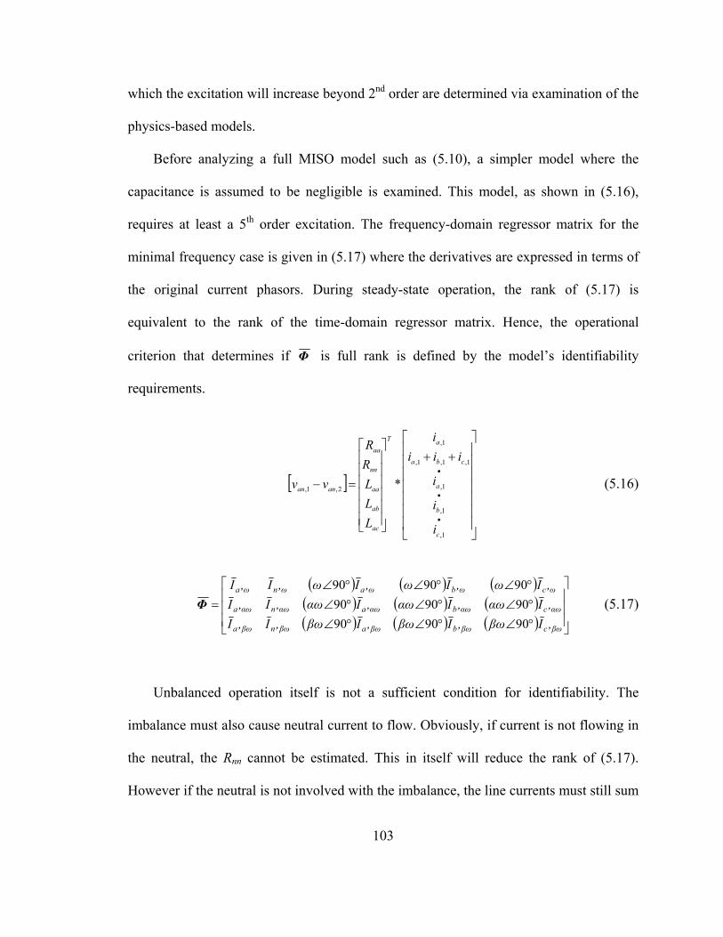
103
which the excitation will increase beyond 2nd order are determined via examination of the
physics-based models.
Before analyzing a full MISO model such as (5.10), a simpler model where the
capacitance is assumed to be negligible is examined. This model, as shown in (5.16),
requires at least a 5th order excitation. The frequency-domain regressor matrix for the
minimal frequency case is given in (5.17) where the derivatives are expressed in terms of
the original current phasors. During steady-state operation, the rank of (5.17) is
equivalent to the rank of the time-domain regressor matrix. Hence, the operational
criterion that determines if Φ is full rank is defined by the model’s identifiability
requirements.
[ ]
⎥⎥⎥⎥⎥⎥⎥
⎦
⎤
⎢⎢⎢⎢⎢⎢⎢
⎣
⎡++
⎥⎥⎥⎥⎥⎥
⎦
⎤
⎢⎢⎢⎢⎢⎢
⎣
⎡
=−
•
•
•
1,
1,
1,
1,1,1,
1,
2,1, *
c
b
a
cba
aT
ac
ab
aa
nn
aa
anan
i
i
i
iiii
LLLRR
vv (5.16)
( ) ( ) ( )
( ) ( ) ( )( ) ( ) ( ) ⎥
⎥⎥
⎦
⎤
⎢⎢⎢
⎣
⎡
°∠°∠°∠°∠°∠°∠°∠°∠°∠
=
βωcβωbβωaβωnβωa
αωcαωbαωaαωnαωa
ωcωbωaωnωa
,Iβω,Iβω,Iβω,I,I,Iαω,Iαω,Iαω,I,I,Iω,Iω,Iω,I,I
909090909090909090
Φ (5.17)
Unbalanced operation itself is not a sufficient condition for identifiability. The
imbalance must also cause neutral current to flow. Obviously, if current is not flowing in
the neutral, the Rnn cannot be estimated. This in itself will reduce the rank of (5.17).
However if the neutral is not involved with the imbalance, the line currents must still sum

104
to zero. Thus, the line currents are linearly dependent by definition. The imbalance must
therefore result from either a fault or load that allows current to flow into the neutral.
Neutral +current alone is also not a sufficient condition either as a balanced fault only
provides a 3rd order excitation.
Excitation requirements for a capacitance only model, such as (5.11), are similar in
nature to that of (5.16). The voltage regressors must contain sufficient harmonic content
as well linear independence in order to provide the necessary excitation. The equivalent
regressor matrix for this model is shown in (5.18). Again, linear dependence between the
regressors is governed by unbalanced system operation that results in current in the
neutral. When no voltage drop occurs in the neutral, the voltages in (5.18) are forced to
sum to zero. Consequently, (5.11)and (5.16) share the same general identifiability
requirements.
( )( ) ( )( ) ( )( )( )( ) ( )( ) ( )( ) ⎥
⎥⎦
⎤
⎢⎢⎣
⎡
−°∠−°∠−°∠−°∠−°∠−°∠
=αωcn,cn,αωbn,bn,αωan,an,
ωcn,cn,ωbn,bn,ωan,an,
,VVα,VVαVVα,VV,VVVV
212121
212121
909090901901901
Φ (5.18)
Models such as (5.10), which consider both the series and shunt terms, will
obviously increase both the required harmonic content as well as the complexity of the
imbalance required. Linear independence between the regressors is additionally
challenging for (5.10) as some type of underlying physical relationship will potentially
exist between the current and voltage based regressors. The associated regressor matrix
for the full model of (5.10) is given in (5.19) through (5.23). The fundamental frequency
term ω was factored out of the derivative terms in order to simplify the expressions.
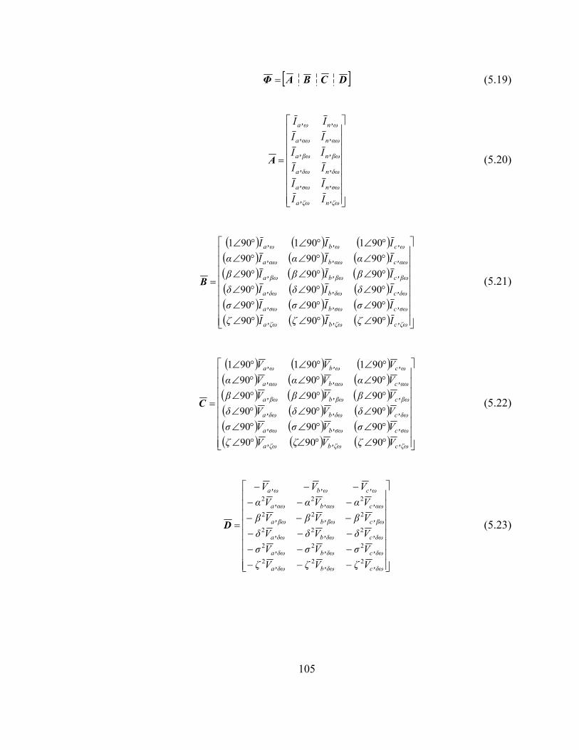
105
[ ]DCBAΦ = (5.19)
⎥⎥⎥⎥⎥⎥⎥⎥
⎦
⎤
⎢⎢⎢⎢⎢⎢⎢⎢
⎣
⎡
=
ζωnζωa
σωnσωa
δωnδωa
βωnβωa
αωnαωa
ωnωa
,I,I,I,I,I,I,I,I,I,I,I,I
A (5.20)
( ) ( ) ( )( ) ( ) ( )( ) ( ) ( )( ) ( ) ( )( ) ( ) ( )( ) ( ) ( ) ⎥
⎥⎥⎥⎥⎥⎥⎥
⎦
⎤
⎢⎢⎢⎢⎢⎢⎢⎢
⎣
⎡
°∠°∠°∠°∠°∠°∠°∠°∠°∠°∠°∠°∠°∠°∠°∠°∠°∠°∠
=
ζωcζωbζωa
σωcσωbσωa
δωcδωbδωa
βωcβωbβωa
αωcαωbαωa
ωcωbωa
,Iζ,Iζ,Iζ,Iσ,Iσ,Iσ,Iδ,Iδ,Iδ,Iβ,Iβ,Iβ,Iα,Iα,Iα,I,I,I
909090909090909090909090909090901901901
B (5.21)
( ) ( ) ( )( ) ( ) ( )( ) ( ) ( )( ) ( ) ( )( ) ( ) ( )( ) ( ) ( ) ⎥
⎥⎥⎥⎥⎥⎥⎥
⎦
⎤
⎢⎢⎢⎢⎢⎢⎢⎢
⎣
⎡
°∠°∠°∠°∠°∠°∠°∠°∠°∠°∠°∠°∠°∠°∠°∠°∠°∠°∠
=
ζωcζωbζωa
σωcσωbσωa
δωcδωbδωa
βωcβωbβωa
αωcαωbαωa
ωcωbωa
,Vζ,Vζ,Vζ,Vσ,Vσ,Vσ,Vδ,Vδ,Vδ,Vβ,Vβ,Vβ,Vα,Vα,Vα,V,V,V
909090909090909090909090909090901901901
C (5.22)
⎥⎥⎥⎥⎥⎥⎥⎥
⎦
⎤
⎢⎢⎢⎢⎢⎢⎢⎢
⎣
⎡
−−−−−−−−−−−−−−−
−−−
=
δωcδωbδωa
δωcδωbδωa
δωcδωbδωa
βωcβωbβωa
αωcαωbαωa
ωcωbωa
,Vζ,Vζ,Vζ,Vσ,Vσ,Vσ,Vδ,Vδ,Vδ,Vβ,Vβ,Vβ,Vα,Vα,Vα
,V,V,V
222
222
222
222
222
D (5.23)
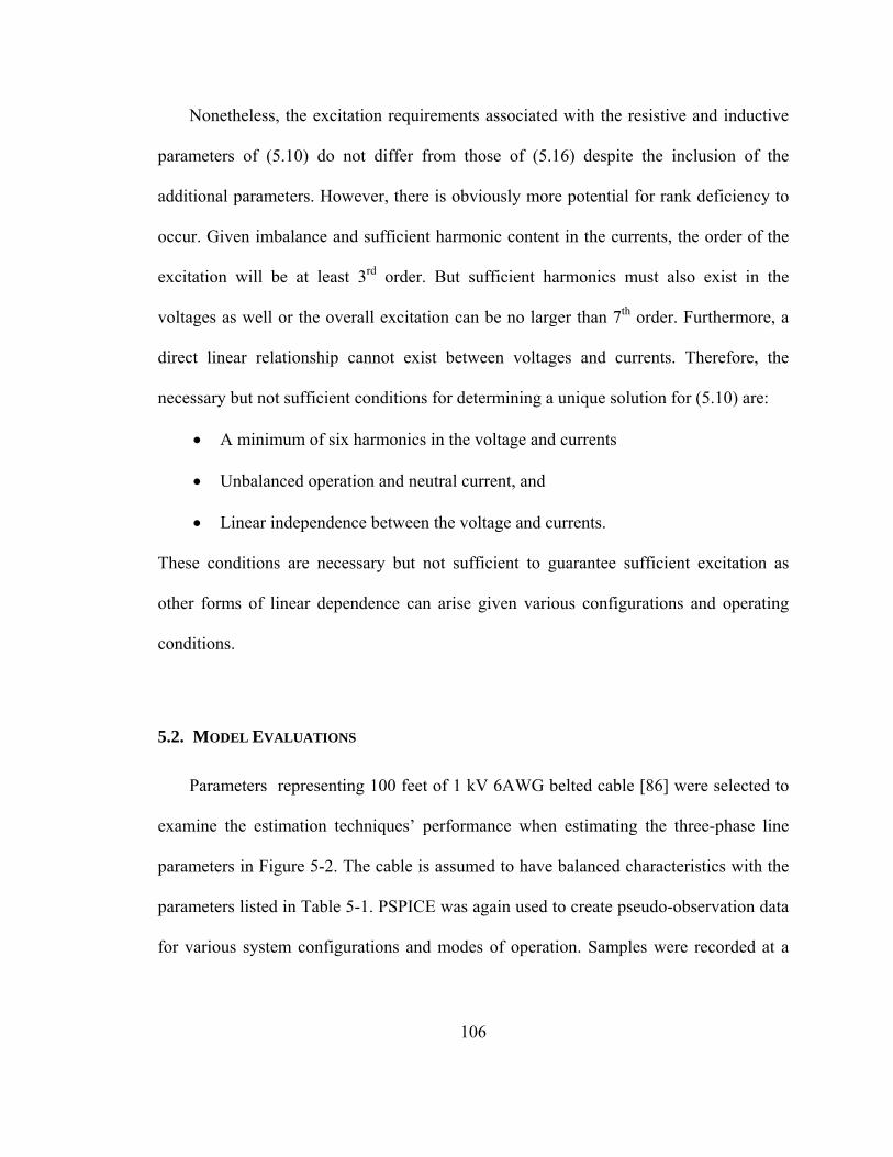
106
Nonetheless, the excitation requirements associated with the resistive and inductive
parameters of (5.10) do not differ from those of (5.16) despite the inclusion of the
additional parameters. However, there is obviously more potential for rank deficiency to
occur. Given imbalance and sufficient harmonic content in the currents, the order of the
excitation will be at least 3rd order. But sufficient harmonics must also exist in the
voltages as well or the overall excitation can be no larger than 7th order. Furthermore, a
direct linear relationship cannot exist between voltages and currents. Therefore, the
necessary but not sufficient conditions for determining a unique solution for (5.10) are:
• A minimum of six harmonics in the voltage and currents
• Unbalanced operation and neutral current, and
• Linear independence between the voltage and currents.
These conditions are necessary but not sufficient to guarantee sufficient excitation as
other forms of linear dependence can arise given various configurations and operating
conditions.
5.2. MODEL EVALUATIONS
Parameters representing 100 feet of 1 kV 6AWG belted cable [86] were selected to
examine the estimation techniques’ performance when estimating the three-phase line
parameters in Figure 5-2. The cable is assumed to have balanced characteristics with the
parameters listed in Table 5-1. PSPICE was again used to create pseudo-observation data
for various system configurations and modes of operation. Samples were recorded at a
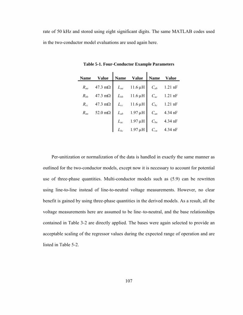
107
rate of 50 kHz and stored using eight significant digits. The same MATLAB codes used
in the two-conductor model evaluations are used again here.
Table 5-1. Four-Conductor Example Parameters
Name Value Name Value Name Value
Raa 47.3 mΩ Laa 11.6 μH Cab 1.21 nF
Rbb 47.3 mΩ Lbb 11.6 μH Cac 1.21 nF
Rcc 47.3 mΩ Lcc 11.6 μH Cbc 1.21 nF
Rnn 52.0 mΩ Lab 1.97 μH Can 4.34 nF
Lac 1.97 μH Cbn 4.34 nF
Lbc 1.97 μH Ccn 4.34 nF
Per-unitization or normalization of the data is handled in exactly the same manner as
outlined for the two-conductor models, except now it is necessary to account for potential
use of three-phase quantities. Multi-conductor models such as (5.9) can be rewritten
using line-to-line instead of line-to-neutral voltage measurements. However, no clear
benefit is gained by using three-phase quantities in the derived models. As a result, all the
voltage measurements here are assumed to be line–to-neutral, and the base relationships
contained in Table 3-2 are directly applied. The bases were again selected to provide an
acceptable scaling of the regressor values during the expected range of operation and are
listed in Table 5-2.

108
Table 5-2. Test System Per-Unit Bases
Base Units Vbase 200 (v) Ibase 20 (A) tbase 2.653 (ms) Sbase 4,000 (VA)Rbase 10 (Ω) Lbase 26.53 (mH)Cbase 265.3 (μF)
The test system is illustrated by Figure 5-3. The three-phase source is modeled by a
set of balanced three-phase voltage sources each with an internal impedance of 3 Ω
connected in grounded wye. The large internal resistance was selected to insure a
sufficient amount of the harmonic currents produced by the rectifier would translate into
voltage harmonics. A three-phase diode bridge rectifier was selected as the load to ensure
enough harmonic content was generated to achieve the necessary excitation conditions.
Figure 5-3. Single Line Diagram of the Three-Phase Test
System
The harmonic currents produced by the rectifier during normal conditions can be
approximated by dividing the fundamental rms current, 1I , by the harmonic number, h, as

109
shown in (5.24) where h = 5, 7, 11, etc. and the even and triplen harmonics are zero. The
chosen 50 kHz sampling rate, however, has a Nyquist frequency of 25 kHz and any
discernable harmonics above this frequency will cause aliasing in the sampled
measurements. Given the small physical values to be estimated, any aliasing can result in
significant bias in the estimations which must be avoided. For the 60 Hz system in Figure
5-3, the first harmonic produced by the rectifier beyond the Nyquist is the 421st harmonic
(25.26 kHz) which is approximately 421hI . While the harmonics beyond the Nyquist
are small in comparison to the fundamental, they must be small enough to not be
detectable from the measurement noise. The quantization error, (3.59), could be used to
determine whether the normally generated harmonics have a strong signal-to-noise ratio
and would be expected to influence the measurements. However, this process cannot
account for transients or other operating conditions which increase the harmonic
magnitudes. Additionally, accurately estimating the small parameter values requires
minimizing the measurement noise which increases the likelihood of detecting these
higher frequencies. Therefore, when designing the monitoring device either the sampling
rate must be set high enough to insure harmonics above the Nyquist frequency cannot be
observed or anti-aliasing filters should be introduced to remove the higher frequency
content. In this case, 2nd order low pass filters with 10 kHz corner frequencies were
introduced during simulation in PSPICE to limit aliasing.
h
II h
1≈ (5.24)

110
The parameter estimation techniques used are exactly the same as those applied for
the two-conductor models. All the conclusions about the estimation techniques’
parameter tracking abilities, convergence, and estimator windup apply to the multi-
conductor models. The main concern with the multi-conductor models then is the
increased difficulties with achieving sufficient excitation.
5.2.1. SERIES ELEMENT MODEL
It is convenient to begin by examining the characteristics of a simple model such as
(5.16). In this case, neither the simulations nor the model included the conductor’s shunt
capacitances. As discussed in the previous section, excitation is limited to 2nd order
during balanced three-phase conditions regardless of the harmonic content. To achieve
independence between the regressors, a 1 Ω resistive fault is introduced at the load
between the a-phase and neutral conductors. The voltage and current waveforms before
and after the fault is introduced, at 250 ms, are given in Figure 5-4. The Fourier series
rms voltages and currents before and after the fault are also provided in Table 5-3
through Table 5-6.

111
Figure 5-4. Test System Voltage and Current Waveforms
(a) Before and (b) After the Fault
Table 5-3. Voltage Fourier Components for Balanced Conditions
HarmonicFourier
Component Phase (Deg)Fourier
Component Phase (Deg)Fourier
Component Phase (Deg)
1 111.51 -1.04 111.51 -121.10 111.51 119.005 6.29 -5.12 6.30 114.70 6.31 -125.107 3.13 -7.37 3.13 -127.30 3.13 112.7011 1.97 168.60 1.97 -71.48 1.97 48.6813 1.40 166.60 1.40 46.46 1.40 -73.4117 0.77 -17.48 0.77 102.50 0.77 -137.4019 0.61 -19.25 0.61 -139.50 0.61 100.70
Phase A Phase B Phase C
Table 5-4. Current Fourier Components for Balanced Conditions
HarmonicFourier
Component Phase (Deg)Fourier
Component Phase (Deg)Fourier
Component Phase (Deg)
1 9.81 -1.10 9.81 -121.10 9.81 118.905 2.07 174.52 2.07 -65.50 2.07 54.507 1.03 172.26 1.03 52.20 1.03 -67.7011 0.65 -12.00 0.65 107.96 0.65 -132.0413 0.46 -14.20 0.46 -134.22 0.46 105.7917 0.25 161.54 0.25 -78.50 0.25 41.5019 0.20 159.54 0.20 39.50 0.20 -80.46
Phase A Phase B Phase C

112
Table 5-5. Voltage Fourier Components for Unbalanced Conditions
HarmonicFourier
Component Phase (Deg)Fourier
Component Phase (Deg)Fourier
Component Phase (Deg)
1 30.94 -1.10 115.33 -125.00 115.33 123.005 1.04 -5.40 2.23 161.50 2.23 -171.507 0.77 172.40 3.01 -64.94 3.02 50.6711 0.37 -12.00 0.79 175.70 0.79 162.1013 0.23 -14.02 0.48 166.60 0.48 167.5017 0.11 161.60 0.84 56.68 0.84 -91.1719 0.17 -20.38 0.40 -172.20 0.40 134.30
Phase A Phase B Phase C
Table 5-6. Current Fourier Components for Unbalanced Conditions
HarmonicFourier
Component Phase (Deg)Fourier
Component Phase (Deg)Fourier
Component Phase (Deg)
1 35.72 -1.10 9.16 -107.33 9.17 105.155 0.36 174.36 0.72 -19.30 0.71 8.407 0.26 -8.00 0.98 113.83 0.98 -129.2111 0.13 167.34 0.25 -5.30 0.25 -19.0013 0.08 165.38 0.16 -14.80 0.15 -13.6017 0.04 -19.20 0.27 -124.32 0.27 87.2119 0.06 158.52 0.13 6.60 0.13 -47.80
Phase A Phase B Phase C
Using RLS with directional forgetting resulted in the parameter estimations given in
Figure 5-5. Before the fault is applied the excitation is insufficient to result in
convergence to a unique solution. Once imbalance is introduced, however, the excitation
rises to sufficient levels for the estimates to converge to their actual values. Additionally,
the margins of error for the estimates, shown in Figure 5-6, indicate a strong level of
confidence for the estimates. It is interesting to note that the resistance, Raa, can be
determined even before the imbalance is introduced. While the individual solutions for
each inductance parameters cannot be determined during balanced conditions, their
influence is still accounted for in the estimates. Analysis of the parameter estimates
during this period confirms that estimates are approximately Laa-Lab ≈ Laa-Lac ≈ 9.64 μH
which is easily shown to be the equivalent positive-sequence inductance.
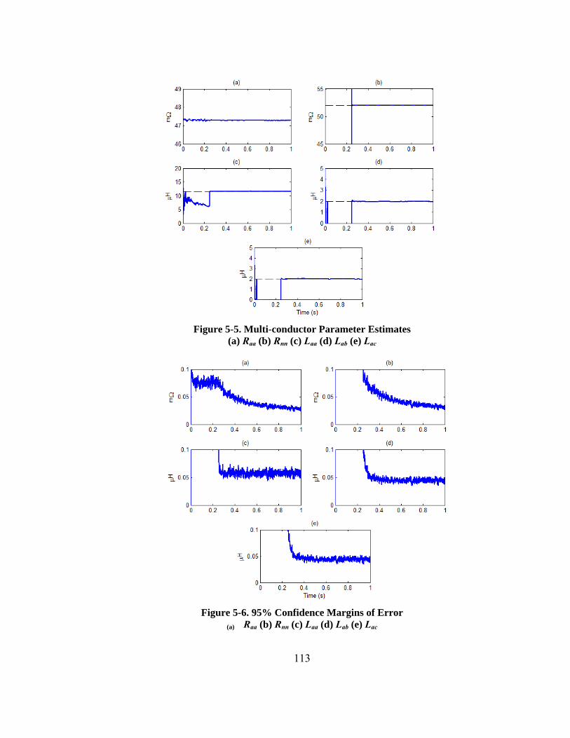
113
Figure 5-5. Multi-conductor Parameter Estimates
(a) Raa (b) Rnn (c) Laa (d) Lab (e) Lac
Figure 5-6. 95% Confidence Margins of Error
(a) Raa (b) Rnn (c) Laa (d) Lab (e) Lac
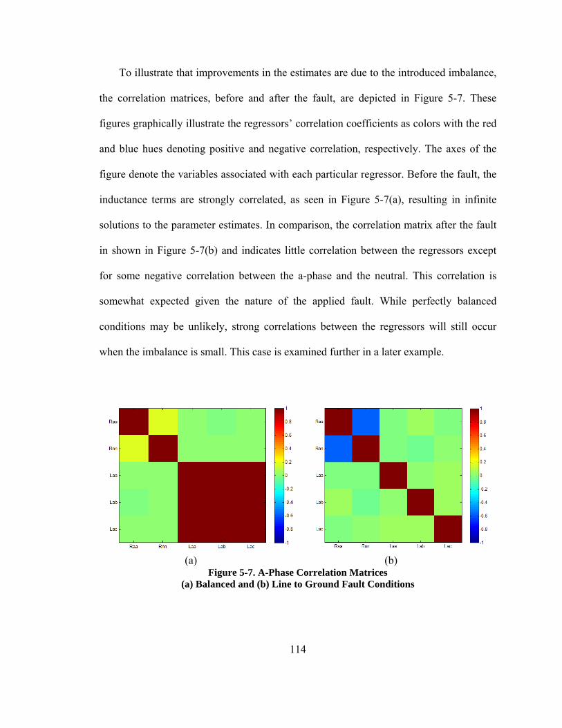
114
To illustrate that improvements in the estimates are due to the introduced imbalance,
the correlation matrices, before and after the fault, are depicted in Figure 5-7. These
figures graphically illustrate the regressors’ correlation coefficients as colors with the red
and blue hues denoting positive and negative correlation, respectively. The axes of the
figure denote the variables associated with each particular regressor. Before the fault, the
inductance terms are strongly correlated, as seen in Figure 5-7(a), resulting in infinite
solutions to the parameter estimates. In comparison, the correlation matrix after the fault
in shown in Figure 5-7(b) and indicates little correlation between the regressors except
for some negative correlation between the a-phase and the neutral. This correlation is
somewhat expected given the nature of the applied fault. While perfectly balanced
conditions may be unlikely, strong correlations between the regressors will still occur
when the imbalance is small. This case is examined further in a later example.
(a) (b)
Figure 5-7. A-Phase Correlation Matrices (a) Balanced and (b) Line to Ground Fault Conditions

115
As previously noted, models for both b and c phases can be written that are similar in
form to (5.10) and can each be estimated using the same sampled data. To illustrate, b-
phase parameter estimates, using the same data as before, are plotted in Figure 5-8. The
estimation of the parameters for the b-phase models using the same data set is important
as it proves the disturbance does not have to occur in a modeled phase. As expected, the
correlation between the b-phase and neutral current is not significant during the fault as
illustrated by the covariance matrix displayed in Figure 5-9.
Figure 5-8. Multi-conductor Parameter Estimates
(a) Rbb (b) Rnn (c) Lbb (d) Lab (e) Lbc
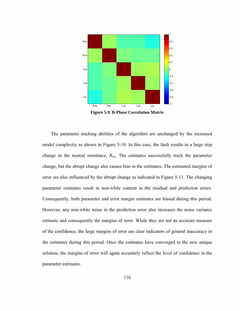
116
Figure 5-9. B-Phase Correlation Matrix
The parameter tracking abilities of the algorithm are unchanged by the increased
model complexity as shown in Figure 5-10. In this case, the fault results in a large step
change in the neutral resistance, Rnn. The estimates successfully track the parameter
change, but the abrupt change also causes bias in the estimates. The estimated margins of
error are also influenced by the abrupt change as indicated in Figure 5-11. The changing
parameter estimates result in non-white content in the residual and prediction errors.
Consequently, both parameter and error margin estimates are biased during this period.
However, any non-white noise in the prediction error also increases the noise variance
estimate and consequently the margins of error. While they are not an accurate measure
of the confidence, the large margins of error are clear indicators of general inaccuracy in
the estimates during this period. Once the estimates have converged to the new unique
solution, the margins of error will again accurately reflect the level of confidence in the
parameter estimates.
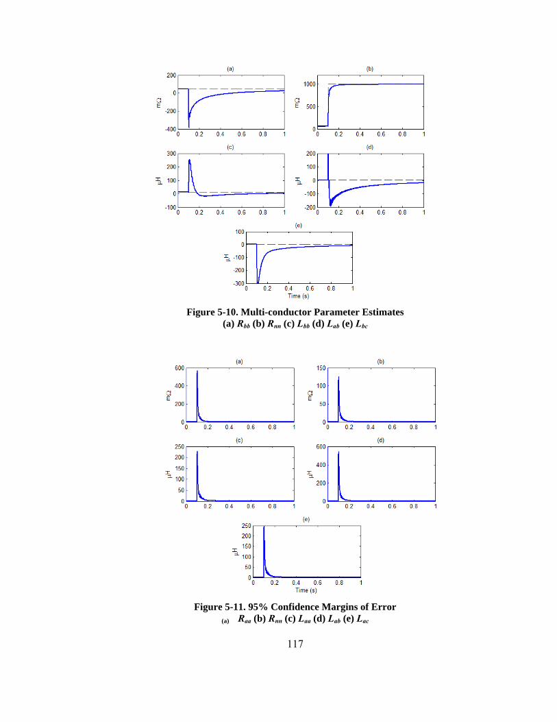
117
Figure 5-10. Multi-conductor Parameter Estimates
(a) Rbb (b) Rnn (c) Lbb (d) Lab (e) Lbc
Figure 5-11. 95% Confidence Margins of Error
(a) Raa (b) Rnn (c) Laa (d) Lab (e) Lac

118
In the next example the excitation provided from a small single phase load is
examined. Instead of the 1 Ω fault, a 20 Ω single phase load is introduced to the a-phase
terminals. Additionally, the load is already in service at the start of the observations.
Therefore, the estimates do not benefit from extra excitation induced by a switching
transient. The resulting parameter estimates are shown in Figure 5-12. As with the line-
to-ground fault example, Raa quickly converged. Yet, the level of independent excitation
provided by the load is not as great as the faulted case, as shown by the correlation matrix
in Figure 5-13. Consequently, the calculated estimations do not converge as quickly. The
influence of multicollinearity is also seen in the margins of error, shown in Figure 5-14,
which are an order of magnitude larger than those in Figure 5-6.
Figure 5-12. Parameter Estimates using RLS/DF
(a) Rcc (b) Rnn (c) Lcc (d) Lac (e) Lbc

119
Figure 5-13. Correlation Matrix for A-phase Estimations
Figure 5-14. 95% Margins of Error (a) Rcc (b) Rnn (c) Lcc (d) Lac (e) Lbc
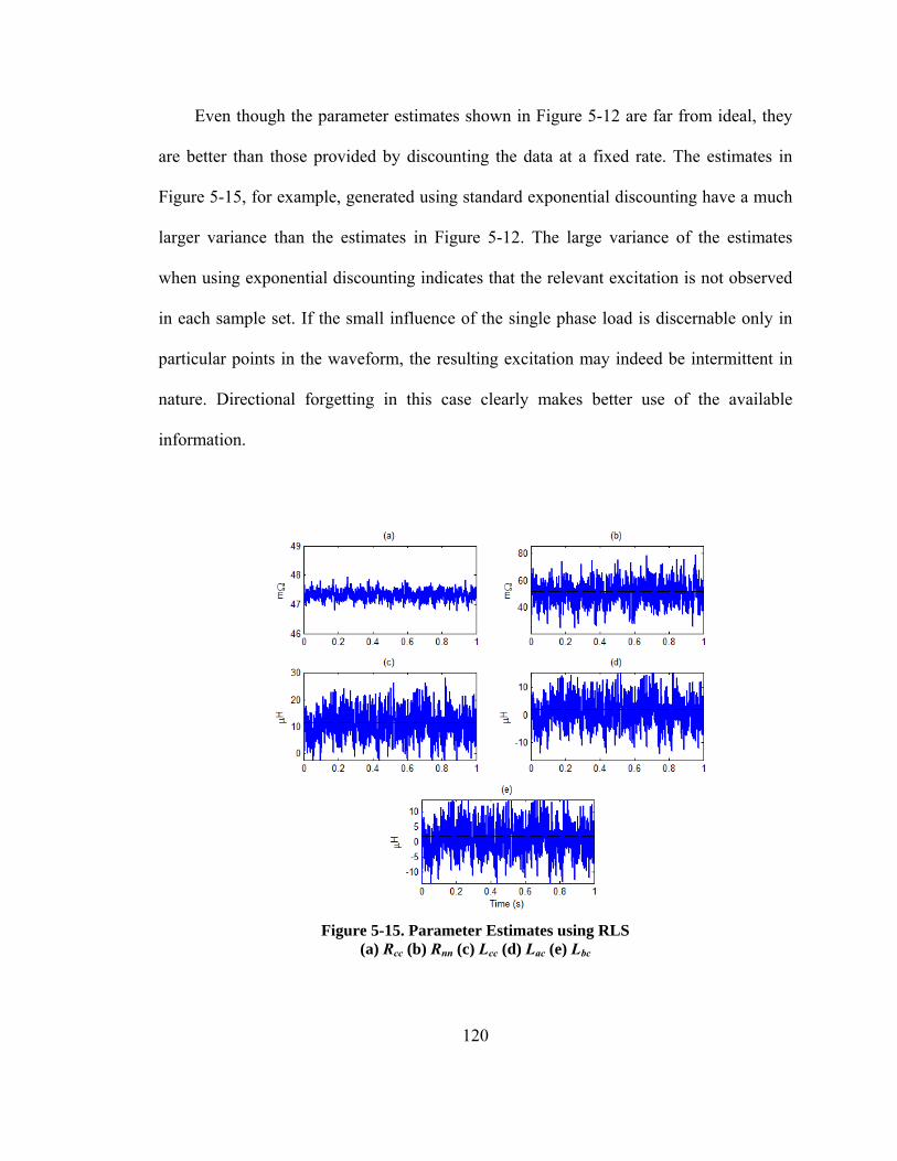
120
Even though the parameter estimates shown in Figure 5-12 are far from ideal, they
are better than those provided by discounting the data at a fixed rate. The estimates in
Figure 5-15, for example, generated using standard exponential discounting have a much
larger variance than the estimates in Figure 5-12. The large variance of the estimates
when using exponential discounting indicates that the relevant excitation is not observed
in each sample set. If the small influence of the single phase load is discernable only in
particular points in the waveform, the resulting excitation may indeed be intermittent in
nature. Directional forgetting in this case clearly makes better use of the available
information.
Figure 5-15. Parameter Estimates using RLS
(a) Rcc (b) Rnn (c) Lcc (d) Lac (e) Lbc

121
5.2.2. SHUNT ELEMENT MODEL
Before returning to the complete four-conductor model of Figure 5-2, estimation of
the capacitances via (5.11) is examined. Estimating capacitance in multiphase lines
displays the same difficulties expressed earlier for the two-conductor models. Namely,
accurate estimation of the relatively small capacitances is influenced by the accuracy of
the measurements. In this example, the PSPICE model was updated to include the
capacitances as well as the resistive and inductive values denoted in Table 5-2 and the
test data was generated using the identical line-to-neutral fault scenario as before. The
ensuing parameter estimates along with each estimated margins of error are documented
in Figure 5-16. As expected, the estimates do not converge until the application of the
fault. Even after the fault occurs, the margins of error do not indicate a strong degree of
confidence in the estimates. In particular, the margins of error for Cab and Cac indicate
little confidence in the estimates. Statistically, it cannot be concluded that these values
are not indeed zero. In diagnostic terms, however, this could also be interpreted as
negligible values. As before, improving the capacitance estimations requires either
reducing the measurement noise or increasing λ.
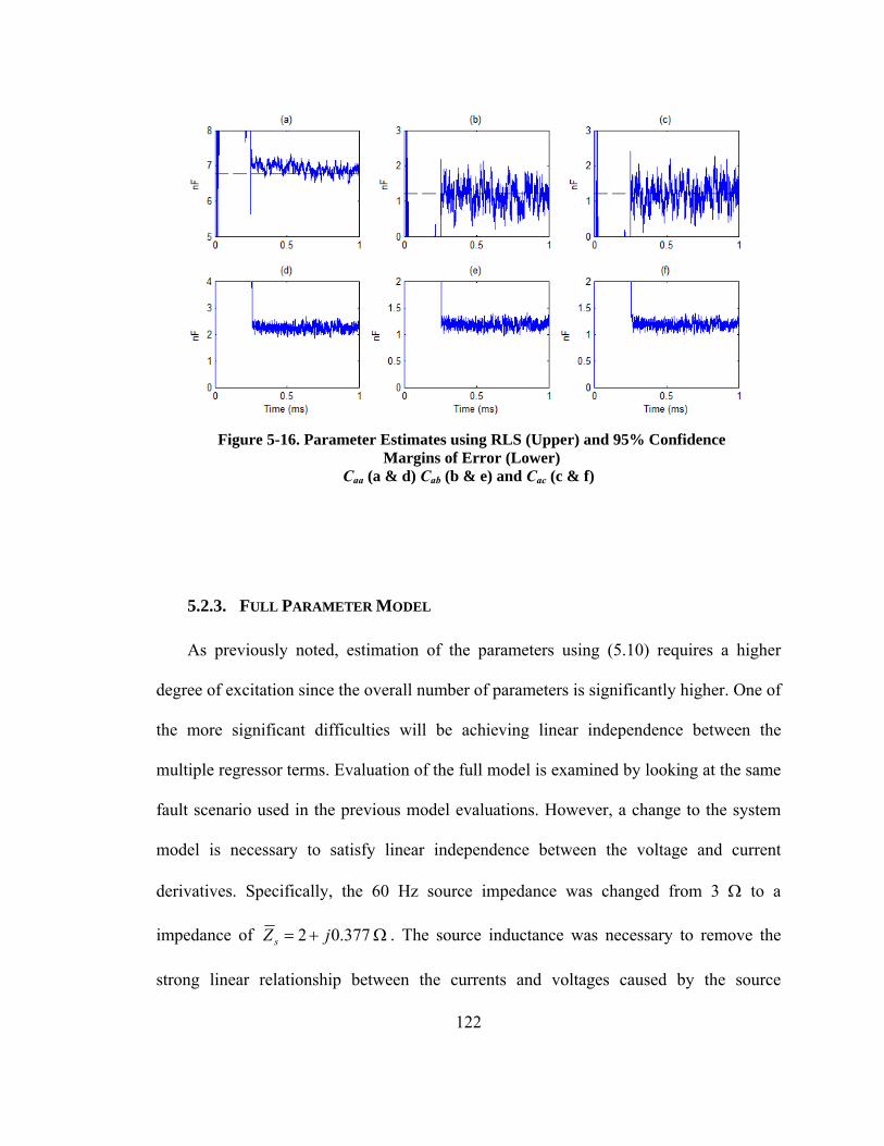
122
Figure 5-16. Parameter Estimates using RLS (Upper) and 95% Confidence
Margins of Error (Lower) Caa (a & d) Cab (b & e) and Cac (c & f)
5.2.3. FULL PARAMETER MODEL
As previously noted, estimation of the parameters using (5.10) requires a higher
degree of excitation since the overall number of parameters is significantly higher. One of
the more significant difficulties will be achieving linear independence between the
multiple regressor terms. Evaluation of the full model is examined by looking at the same
fault scenario used in the previous model evaluations. However, a change to the system
model is necessary to satisfy linear independence between the voltage and current
derivatives. Specifically, the 60 Hz source impedance was changed from 3 Ω to a
impedance of Ω+= 377.02 jZs . The source inductance was necessary to remove the
strong linear relationship between the currents and voltages caused by the source

123
resistance. The resulting parameters estimates are shown in Figure 5-17 and the
corresponding margins of error are shown in Figure 5-18. The results demonstrate many
of the expected difficulties with the model including the fact that the RC and LC terms do
not converge to acceptable values. Still, once the fault occurs, the resistance and
inductance estimates converge to within acceptable ranges. The large margins of error in
Figure 5-18 are an indication that many of the parameters estimated by the full model
may be unnecessary. Therefore, the same parameter set is used to fit the model in (5.16).
As shown in Figure 5-19, the estimates using this model show little signs of bias due to
minimal influence of the capacitances.

124
Figure 5-17. Parameter Estimates using RLS/DF
(a) Raa (b) Rnn (c) Laa (d) Lab (e) Lac (f) RaaCaa+RnnCnn (g) -RaaCab+RnnCbn (h) -RaaCac+RnnCcn (i) LaaCaa-LabCab-LacCac (j) LabCbb-LaaCab-LacCbc
(k) LacCcc-LaaCac-LabCbc

125
Figure 5-18. 95% Confidence Margins of Error
(a) Raa (b) Rnn (c) Laa (d) Lab (e) Lac (f) RaaCaa+RnnCnn (g) -RaaCab+RnnCbn (h) -RaaCac+RnnCcn (i) LaaCaa-LabCab-LacCac (j) LabCbb-
LaaCab-LacCbc (k) LacCcc-LaaCac-LabCbc
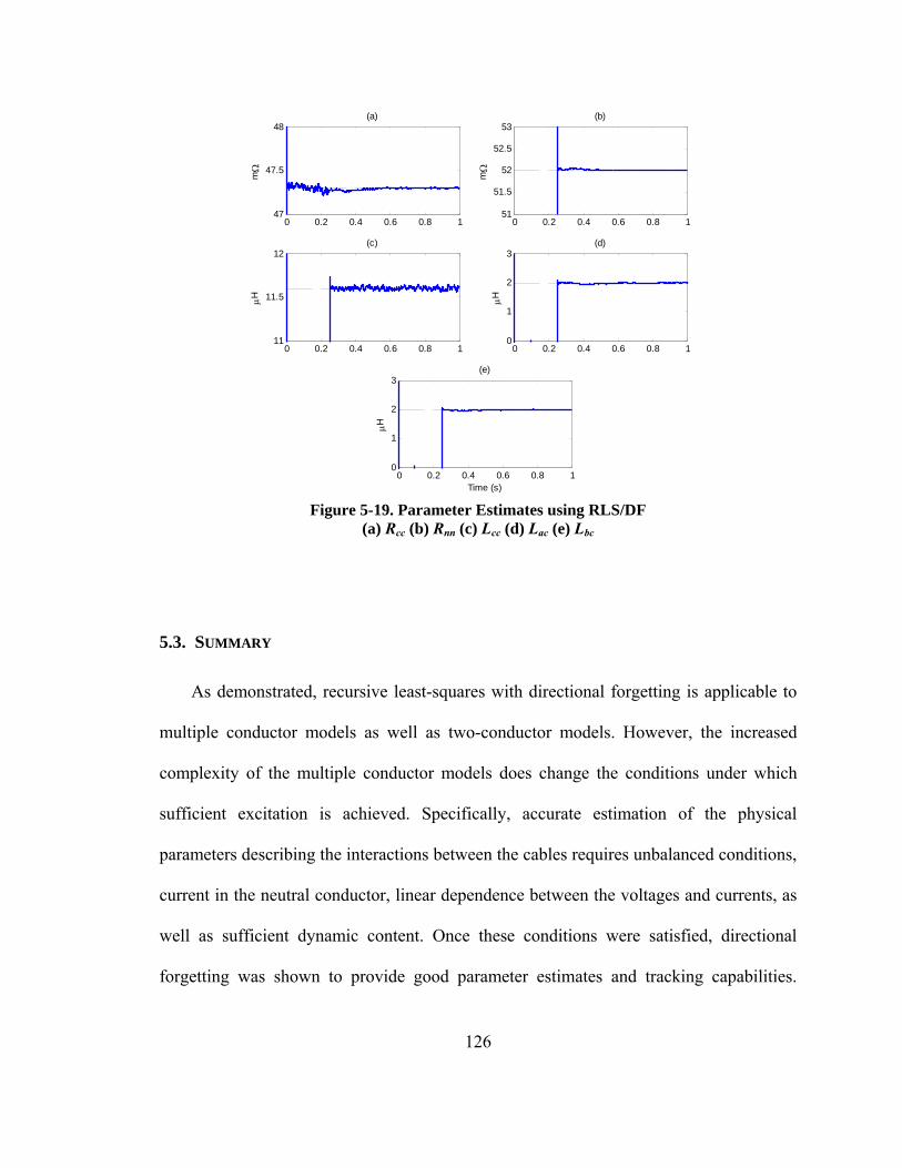
126
0 0.2 0.4 0.6 0.8 147
47.5
48(a)
mΩ
0 0.2 0.4 0.6 0.8 151
51.5
52
52.5
53(b)
mΩ
0 0.2 0.4 0.6 0.8 111
11.5
12(c)
μH
0 0.2 0.4 0.6 0.8 10
1
2
3(d)
μH
0 0.2 0.4 0.6 0.8 10
1
2
3(e)
Time (s)
μH
Figure 5-19. Parameter Estimates using RLS/DF
(a) Rcc (b) Rnn (c) Lcc (d) Lac (e) Lbc
5.3. SUMMARY
As demonstrated, recursive least-squares with directional forgetting is applicable to
multiple conductor models as well as two-conductor models. However, the increased
complexity of the multiple conductor models does change the conditions under which
sufficient excitation is achieved. Specifically, accurate estimation of the physical
parameters describing the interactions between the cables requires unbalanced conditions,
current in the neutral conductor, linear dependence between the voltages and currents, as
well as sufficient dynamic content. Once these conditions were satisfied, directional
forgetting was shown to provide good parameter estimates and tracking capabilities.

127
Directional forgetting was also shown to provide good estimates when the intermittency
is increased by strong correlations between the measurements, as evidenced in Figure
4-12. The proposed methods show good results using time-domain measurements and
models of both two and multiple conductor models. Estimation of network parameter
using frequency-domain measurements and models is examined in Chapter 6.

128
CHAPTER 6
FREQUENCY-DOMAIN MODELS
The estimation and tracking techniques utilized in the time domain models are
equally applicable to frequency-domain models. In fact, sufficient excitation can be more
difficult to achieve in the steady-state frequency domain as the excitation cannot be
increased through additional harmonic content. Consequently, excitation can only occur
through changes in the phasor values over time. While the nature of the excitation is
different between time-domain and frequency domain, the requirements of the estimation
methods are unchanged. In this chapter, estimation of network characteristics using
frequency-domain measurements is examined. While the line parameters can be
indentified using frequency-domain measurements, estimation and tracking of the
Thevenin equivalent provides the most benefit by allowing monitoring of network
characteristics even with limited measurements.
6.1. LINE MODELS
An equivalent frequency domain model can be derived for all of the time-domain
models presented in Chapters 4 and 5. The two-conductor MISO model equivalent is
provided in (6.1) - (6.4). There are still four unknown parameters, the real and imaginary
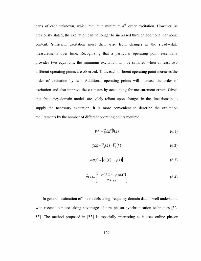
129
parts of each unknown, which require a minimum 4th order excitation. However, as
previously stated, the excitation can no longer be increased through additional harmonic
content. Sufficient excitation must then arise from changes in the steady-state
measurements over time. Recognizing that a particular operating point essentially
provides two equations, the minimum excitation will be satisfied when at least two
different operating points are observed. Thus, each different operating point increases the
order of excitation by two. Additional operating points will increase the order of
excitation and also improve the estimates by accounting for measurement errors. Given
that frequency-domain models are solely reliant upon changes in the time-domain to
supply the necessary excitation, it is more convenient to describe the excitation
requirements by the number of different operating points required.
( )k(k)(k)y Tθϕ~~= (6.1)
( ) ( )kVkV(k)y SR −= (6.2)
( ) ( )[ ]kIkV(k) SST =ϕ~ (6.3)
( ) ( ) ( )⎥⎦
⎤⎢⎣
⎡
++−
=jXR
LCjRCk ωωθ
2~ (6.4)
In general, estimation of line models using frequency domain data is well understood
with recent literature taking advantage of new phasor synchronization techniques [52,
53]. The method proposed in [53] is especially interesting as it uses online phasor
130
measurements to determine both the positive and zero sequence impedances.
Furthermore, the excitation requirements mirror those determined for the multi-conductor
models. Specifically, synchronized phasor measurements obtained during ground faults
were needed to estimate the zero sequence impedance and mutual coupling terms.
Estimation of the models in [53] was performed using least-squares, (3.5), and a
minimal number of measurements. Tracking capabilities could be added by using RLS
with some form of discounting as the estimation method. Recalling that parameter drift
(estimator windup) is a function of solution method and not the data type, retention of
sufficiently exciting information is still an important issue. This is especially true for line
models at frequencies other than the fundamental where the excitation is dependent on
factors such as harmonic injections and system configuration. As repeated measurement
of the same operating conditions does not provide additional information at any
frequency, intermittency can occur even at the fundamental frequency. In general,
directional forgetting RLS is beneficial to any online automated application where the
excitation is potentially intermittent.
6.2. THEVENIN EQUIVALENT
Measurements at both terminals of a branch in the network are not always possible;
however, some form of evaluating the network health is still desirable. In these cases,
tracking the Thevenin equivalent provides potentially useful information about the
network or device. Before examining steady-state approaches using frequency domain

131
measurements it is enlightening to first examine estimation of the Thevenin equivalent in
the time domain.
6.2.1. TIME-DOMAIN
Time-domain information can be used to estimate the Thevenin equivalent at each
frequency, but the estimates are interdependent on the selected impedance model. For
example, assume that the time-domain model in (6.5) is used to model the fundamental
frequency Thevenin equivalent using time-domain voltage and current measurements (v
and i). In this case, it is assumed that the R and L components are adequate to represent
the Thevenin impedances over all observed frequencies. Additionally, a and b parameters
are introduced to estimate the real and imaginary parts of the open-circuit voltage through
the inclusion of the cos(ωt) and sin(ωt) regressors where ω is the radian frequency for the
modeled voltage source. In this formulation the reference angle is defined by cos(ωt) and
the phase angle of the terminal voltage can be found by estimating the terminal voltage
phasor using (6.6).
[ ] ( ) ( )[ ]TttiibaLRv ωω sincos* &= (6.5)
[ ] ( ) ( )[ ]TIR ttVVv ωω sincos*= (6.6)
When a constant fundamental frequency current and voltage are observed, the
excitation is insufficient to provide a converged solution. If the excitation is increased by
a transient or harmonic, the Thevenin equivalent can be estimated. However, if the
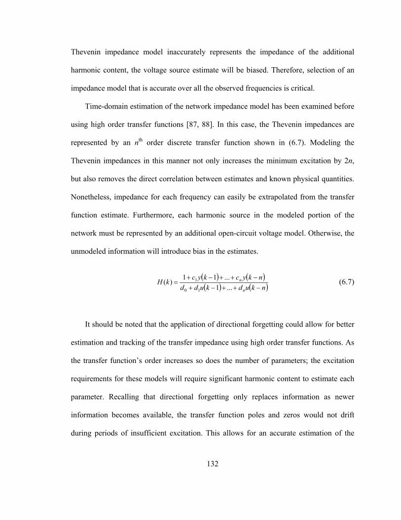
132
Thevenin impedance model inaccurately represents the impedance of the additional
harmonic content, the voltage source estimate will be biased. Therefore, selection of an
impedance model that is accurate over all the observed frequencies is critical.
Time-domain estimation of the network impedance model has been examined before
using high order transfer functions [87, 88]. In this case, the Thevenin impedances are
represented by an nth order discrete transfer function shown in (6.7). Modeling the
Thevenin impedances in this manner not only increases the minimum excitation by 2n,
but also removes the direct correlation between estimates and known physical quantities.
Nonetheless, impedance for each frequency can easily be extrapolated from the transfer
function estimate. Furthermore, each harmonic source in the modeled portion of the
network must be represented by an additional open-circuit voltage model. Otherwise, the
unmodeled information will introduce bias in the estimates.
( ) ( )( ) ( )nkudkudd
nkyckyckHn
n
−++−+−++−+
=...1
...11)(10
1 (6.7)
It should be noted that the application of directional forgetting could allow for better
estimation and tracking of the transfer impedance using high order transfer functions. As
the transfer function’s order increases so does the number of parameters; the excitation
requirements for these models will require significant harmonic content to estimate each
parameter. Recalling that directional forgetting only replaces information as newer
information becomes available, the transfer function poles and zeros would not drift
during periods of insufficient excitation. This allows for an accurate estimation of the
133
transfer impedance even when the chosen model is over-parameterized. Thus, higher
order models could be used to improve the results in [87]. However, it is unclear how the
past information might bias the general shape of the transfer impedance when network
changes occur and an incomplete harmonic spectrum is available.
Unmodeled frequencies could be filtered from the observations to eliminate the
influence of the transfer impedance model. For instance, all but the fundamental
frequency could theoretically be removed from the data used to fit the model in (6.5). In
this case, sufficient excitation is only achieved by changes in the fundamental frequency
content. Note that there are four unknown parameters but two are associated with
regressors representing steady-state values. At least one outside change in the current
regressor terms is required for sufficient excitation. This formulation is analogous to a
frequency domain approach.
6.2.2. FREQUENCY-DOMAIN
While estimation of the Thevenin equivalent is possible in the time domain, there are
several reasons why it may be an unattractive approach:
• Difficulties in defining an accurate model,
• Design and implementation of multiple filters,
• Availability of time-domain measurements, and
• Measurements must be sampled at a fixed rate
An alternative is to use steady-state phasor measurements to independently estimate the
Thevenin equivalent at each frequency. In this approach, methods for providing the
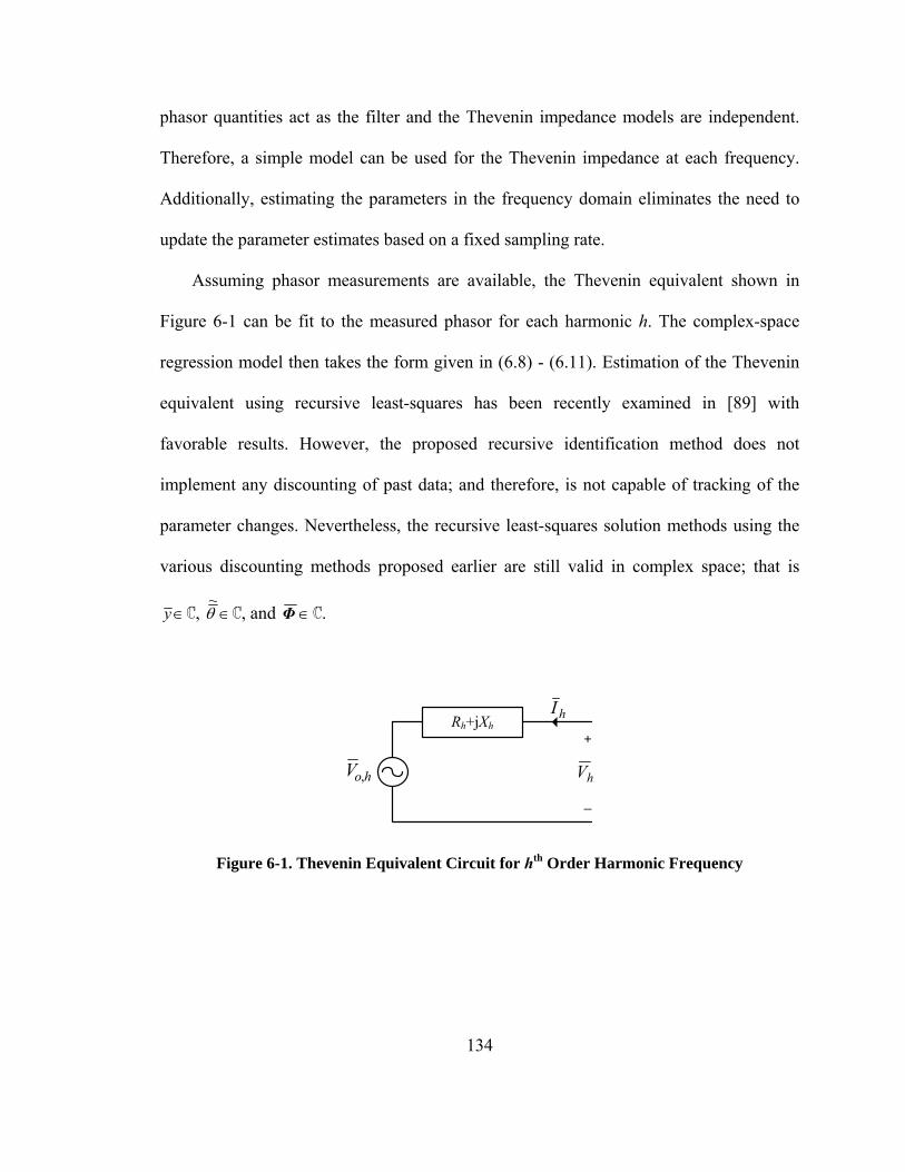
134
phasor quantities act as the filter and the Thevenin impedance models are independent.
Therefore, a simple model can be used for the Thevenin impedance at each frequency.
Additionally, estimating the parameters in the frequency domain eliminates the need to
update the parameter estimates based on a fixed sampling rate.
Assuming phasor measurements are available, the Thevenin equivalent shown in
Figure 6-1 can be fit to the measured phasor for each harmonic h. The complex-space
regression model then takes the form given in (6.8) - (6.11). Estimation of the Thevenin
equivalent using recursive least-squares has been recently examined in [89] with
favorable results. However, the proposed recursive identification method does not
implement any discounting of past data; and therefore, is not capable of tracking of the
parameter changes. Nevertheless, the recursive least-squares solution methods using the
various discounting methods proposed earlier are still valid in complex space; that is
∈y ℂ, ∈θ~
ℂ, and ∈Φ ℂ.
Rh+jXh+
_
hoV ,
hI
hV
Figure 6-1. Thevenin Equivalent Circuit for hth Order Harmonic Frequency
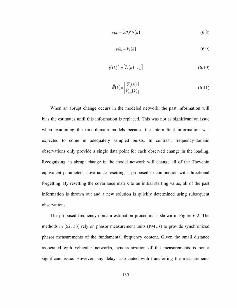
135
( )k(k)(k)y Tθϕ~~= (6.8)
( )kV(k)y h= (6.9)
( )[ ]hhT ckIk =)(~ϕ (6.10)
( ) ( )( )⎥⎦
⎤⎢⎣
⎡=
kVkZ
ko,h
hθ~
(6.11)
When an abrupt change occurs in the modeled network, the past information will
bias the estimates until this information is replaced. This was not as significant an issue
when examining the time-domain models because the intermittent information was
expected to come in adequately sampled bursts. In contrast, frequency-domain
observations only provide a single data point for each observed change in the loading.
Recognizing an abrupt change in the model network will change all of the Thevenin
equivalent parameters, covariance resetting is proposed in conjunction with directional
forgetting. By resetting the covariance matrix to an initial starting value, all of the past
information is thrown out and a new solution is quickly determined using subsequent
observations.
The proposed frequency-domain estimation procedure is shown in Figure 6-2. The
methods in [52, 53] rely on phasor measurement units (PMUs) to provide synchronized
phasor measurements of the fundamental frequency content. Given the small distance
associated with vehicular networks, synchronization of the measurements is not a
significant issue. However, any delays associated with transferring the measurements
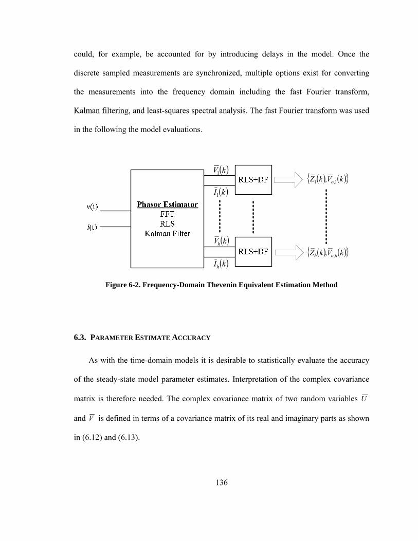
136
could, for example, be accounted for by introducing delays in the model. Once the
discrete sampled measurements are synchronized, multiple options exist for converting
the measurements into the frequency domain including the fast Fourier transform,
Kalman filtering, and least-squares spectral analysis. The fast Fourier transform was used
in the following the model evaluations.
( )kV1
( )kI1
( )kVh
( )kIh
( ) ( ){ }kVkZ o 1,1 ,
( ) ( ){ }kVkZ hoh ,,
Figure 6-2. Frequency-Domain Thevenin Equivalent Estimation Method
6.3. PARAMETER ESTIMATE ACCURACY
As with the time-domain models it is desirable to statistically evaluate the accuracy
of the steady-state model parameter estimates. Interpretation of the complex covariance
matrix is therefore needed. The complex covariance matrix of two random variables U
and V is defined in terms of a covariance matrix of its real and imaginary parts as shown
in (6.12) and (6.13).

137
( ) ( ) ( ) ( ) ( )( )IRRIIIRR VUVUjVUVUV,U ,cov,cov,cov,covcov +++= (6.12)
( ) ( ) ( ) ( ) ( )
( ) ( ) ( ) ( )( ) ( ) ( ) ( )
( ) ( ) ( ) ( ) ⎥⎦
⎤⎢⎣
⎡−−−−
+⎥⎦
⎤⎢⎣
⎡++++
=
RIIRRI
IRRIRI
IRIIRR
IIRRIR
VVVUVUVUVUUU
j
VVVUVUVUVUUU
V,U
varvar,cov,cov,cov,covvarvar
*
varvar,cov,cov,cov,covvarvar
cov (6.13)
The least-squares matrices P and R are positive definite, so the diagonal terms of the
covariance matrix are always positive real values. If (6.13) is also positive definite, the
variance of the real and imaginary parts of the complex random variables U and V must
be equal. The covariance matrix shown in (6.13) also demonstrates that the real diagonal
entries of P are indicative of the variance of only the complex random variable associated
with each regressor. Additionally, it agrees with a common definition of the complex
random variable variance given in (6.14). Therefore, the real numbers contained in the
diagonal entries of P directly indicate the variance of the phasor magnitude as defined by
(6.15).
[ ]( ) [ ]( )[ ] )var()var(*)var( *IR zzZEZZEZEZ +=−−= (6.14)
( ) ( ) ( )( ) ( ) ( ) 22
211
2
2var2varvar
2var2varvar
PVVV
PUUU
IR
IR
σ
σ
===
=== (6.15)
The prediction error is also a complex random variable. The residual variance can
still be estimated using (3.52) but the variance of the real and imaginary portions of the
prediction error must be determined separately as shown in (6.16) and (6.17). The
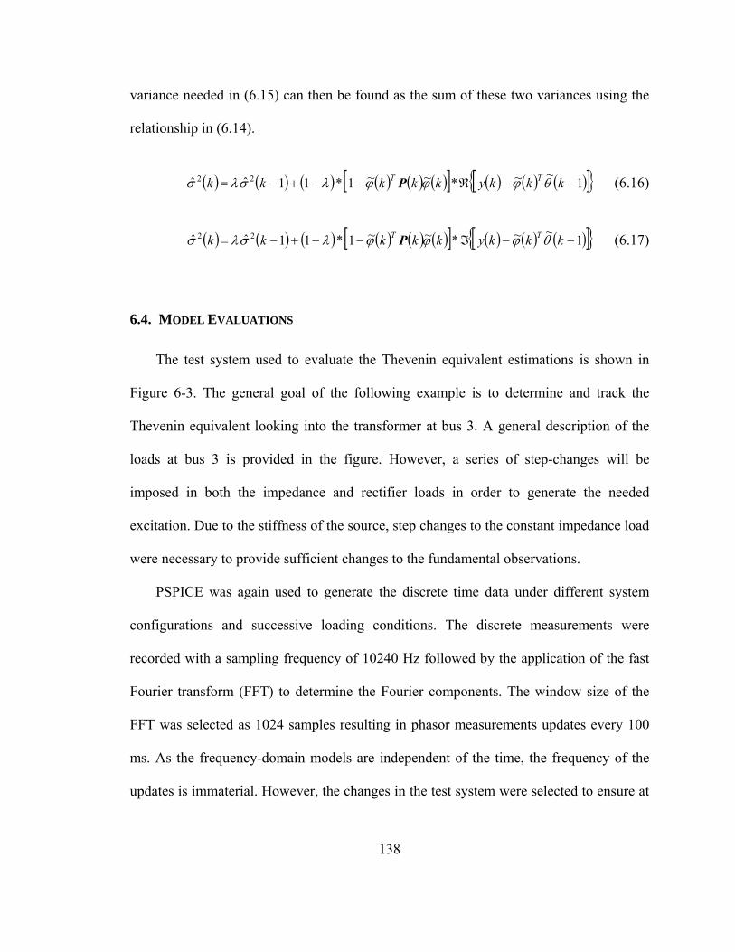
138
variance needed in (6.15) can then be found as the sum of these two variances using the
relationship in (6.14).
( ) ( ) ( ) ( ) ( ) ( )[ ] ( ) ( ) ( )[ ]{ }1~~*~~1*11ˆˆ 22 −−ℜ−−+−= kkkykkkkk TT θϕϕϕλσλσ P (6.16)
( ) ( ) ( ) ( ) ( ) ( )[ ] ( ) ( ) ( )[ ]{ }1~~*~~1*11ˆˆ 22 −−ℑ−−+−= kkkykkkkk TT θϕϕϕλσλσ P (6.17)
6.4. MODEL EVALUATIONS
The test system used to evaluate the Thevenin equivalent estimations is shown in
Figure 6-3. The general goal of the following example is to determine and track the
Thevenin equivalent looking into the transformer at bus 3. A general description of the
loads at bus 3 is provided in the figure. However, a series of step-changes will be
imposed in both the impedance and rectifier loads in order to generate the needed
excitation. Due to the stiffness of the source, step changes to the constant impedance load
were necessary to provide sufficient changes to the fundamental observations.
PSPICE was again used to generate the discrete time data under different system
configurations and successive loading conditions. The discrete measurements were
recorded with a sampling frequency of 10240 Hz followed by the application of the fast
Fourier transform (FFT) to determine the Fourier components. The window size of the
FFT was selected as 1024 samples resulting in phasor measurements updates every 100
ms. As the frequency-domain models are independent of the time, the frequency of the
updates is immaterial. However, the changes in the test system were selected to ensure at

139
least ten sample points of the same phasors were generated for each change in the
loading. The equivalent memory size was also decreased, by fixing λ = 0.9, to
sufficiently test the directional forgetting algorithm.
Figure 6-3. Single-Phase Test Network
Evaluation of parameter tracking ability is tested by alteration of the Thevenin
equivalent via the switched capacitor located at bus 1. The capacitor is switched into
service during the simulation corresponding to reactive compensation at the substation. A
frequency scan of the transfer impedance looking into the network with and without the
capacitor in service is shown in Figure 6-4. While the diode rectifier generates numerous
odd harmonics, it is not necessary to fit a model for every harmonic. Instead, only those
harmonic frequencies listed in Table 6-1, along with their relevant Thevenin equivalent
values, are evaluated.
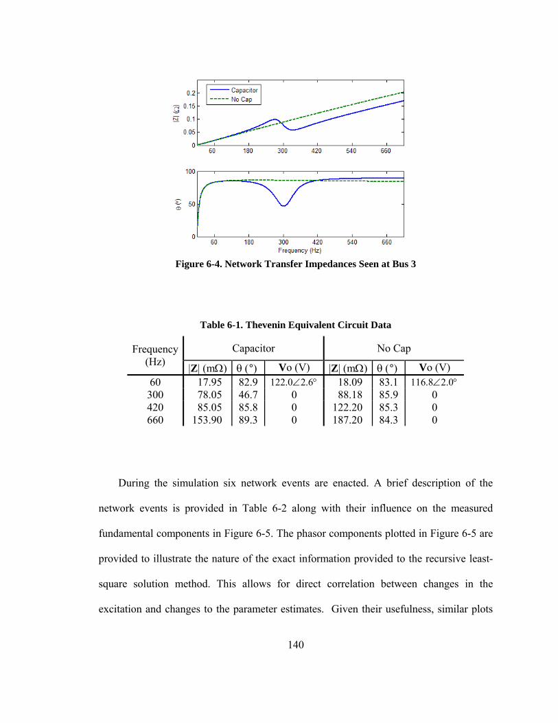
140
Figure 6-4. Network Transfer Impedances Seen at Bus 3
Table 6-1. Thevenin Equivalent Circuit Data
Capacitor No Cap Frequency (Hz) |Z| (mΩ) θ (°) Vo (V) |Z| (mΩ) θ (°) Vo (V) 60 17.95 82.9 °∠ 6.20.122 18.09 83.1 °∠ 0.28.116300 78.05 46.7 0 88.18 85.9 0 420 85.05 85.8 0 122.20 85.3 0 660 153.90 89.3 0 187.20 84.3 0
During the simulation six network events are enacted. A brief description of the
network events is provided in Table 6-2 along with their influence on the measured
fundamental components in Figure 6-5. The phasor components plotted in Figure 6-5 are
provided to illustrate the nature of the exact information provided to the recursive least-
square solution method. This allows for direct correlation between changes in the
excitation and changes to the parameter estimates. Given their usefulness, similar plots

141
will be provided for each harmonic model evaluated. The terminal voltage, V , is used as
the reference for each harmonic and therefore VI is zero at each instant and not plotted.
Table 6-2. Test System Events
Event # Description 1 Switching in of Load 2 2 Three successive increases to Load 3 3 Step increase in Load 2 4 Switching in of capacitor at Bus 1 5 Removal of Load 2 6 Three successive decreases to Load 3
Figure 6-5. Input-Output Phasor Components at 60 Hz
Estimation of the complex space model (6.8)-(6.11) was performed using RLS with
directional forgetting and covariance resetting. Resetting the covariance matrix was
selected to occur whenever the prediction error was larger than 20%. Tracking small

142
variations in the Thevenin equivalent was provided for by selecting a value for λ of 0.99.
The resulting parameter estimates are illustrated in Figure 6-6.
As expected, the estimates do not start to show signs of convergence until the second
operating point. Still, the inaccuracy resulting from the flat start and the initial
insufficient conditions results in a large prediction error causing the resetting of the
covariance matrix as indicated in Figure 6-7. The next event to occur consists of step
changes in the rectifier load which increases the real power demand of the rectifier.
However, the resetting of the covariance matrix results in little confidence in the current
parameter estimates at this point. Therefore, when changes occur only in IR but not in II,
as shown in Figure 6-5, the past excitation is insufficient to provide a good estimate of the
Thevenin equivalent. Effectively, the regressor II is constant over all the retained
observations and therefore linearly dependent with the constant voltage source regressors.
Consequently, the Thevenin impedance is interpreted as being entirely real as indicated
by the angle of the estimated impedance. This suggests that this method cannot be
applied to estimate the Thevenin equivalent seen by a purely real or inductive load. Still
when the inductive load increases during event #3, the change is observed in both phasor
components. As a result, the excitation contained in all the regressors is sufficient for the
solution to converge to reasonable estimates.
The estimates are accurate until the Thevenin equivalent is altered by the capacitor
switching at bus 1. The abrupt change in the network model results in a large prediction
error which again triggers the resetting of the covariance matrix. By discounting all of the
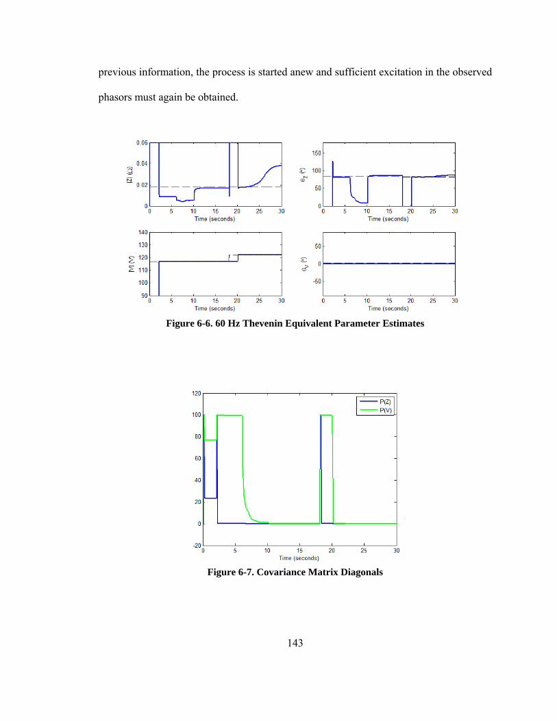
143
previous information, the process is started anew and sufficient excitation in the observed
phasors must again be obtained.
Figure 6-6. 60 Hz Thevenin Equivalent Parameter Estimates
Figure 6-7. Covariance Matrix Diagonals

144
The same test system and procedures were applied to the 5th harmonic (300Hz)
measurements shown in Figure 6-8. Examination of the phasor components at this
frequency indicates that the changes in load 2 have very little influence on the 5th
harmonic content. Hence, rectifier load changes are the sole source of excitation for the
Thevenin equivalent model at this frequency. Nonetheless, the Thevenin equivalent
estimations shown in Figure 6-9 demonstrate that the method provides good estimation
and tracking properties in response to the load changes. Note that estimations accurately
reflect the lack of a voltage source at this frequency in the modeled network. Similar
examples can be generated for any of the harmonics observed in the network.
Figure 6-8. Input-Output Phasor Components at 300 Hz

145
Figure 6-9. 300 Hz Thevenin Equivalent Parameter Estimates
6.5. SUMMARY
Continuous online estimation of the Thevenin equivalent provides a powerful tool
from which to characterize the network and system components. This is especially true
when only terminal measurements are available for some devices. The proposed
frequency-domain methods have been shown to provide good parameter estimation and
tracking abilities under the intermittent conditions. The parameter estimation methods
given in Chapter 3 were also shown to require minimal changes when applied to complex
numbers. Depending of the available measurements, the frequency-domain and time-
domain parameter estimation techniques can provide sufficiently accurate estimates
needed to monitor the health of not only individual devices but the overall network health
as well.

146
CHAPTER 7
CONCLUSIONS
Parameter estimation techniques suitable to online estimation and tracking of
network parameters under the assumed monitoring procedures have been presented. As
the excitation is uncontrolled but must be sufficient to determine the characteristics of
interest, the presented recursive least-squares methods were examined under the
assumption that the excitation is intermittently spaced over time. These techniques have
shown good estimation and tracking properties under the assumed conditions and will
serve as the foundation for subsequent development of online model-based condition
monitors. As the nature of the intermittency is also intrinsically linked to the chosen
model, the techniques were evaluated and shown to be effective for multiple models in
both the time and frequency domains.
7.1. SUMMARY
The recursive least-squares techniques were presented and examined in detail in
Chapter 3. In order to follow time-varying parameters, the estimation method must
discount past data in favor of more recently sampled information. The recursive least-
squares method augmented with directional forgetting was proposed to provide better

147
retention of the intermittent information while still providing tracking capabilities.
Variable directional forgetting and covariance resetting were also introduced to increase
tracking capabilities of the method when large abrupt parameter changes occur.
As sufficient excitation cannot be guaranteed by the monitoring method, statistical
measures in the form of confidence intervals, multicollinearity tests, and residual analysis
were introduced to gauge the accuracy of the estimates. Additionally, the online statistical
measures were designed to require minimal additional computation effort. The accuracy
of the estimation is also intrinsically tied to the accuracy of the sample data. Design
criteria for the filtering and the A/D conversion process governing the accuracy of the
estimation algorithms were also documented.
Identifiability of the modeled parameters is not only determined by the solution
method and the observed sample measurements but by the model as well. The
identifiability requirements of two-conductor lines were examined in Chapter 4. Standard
models representing different assumptions about the line and available measurements
were developed in forms allowing for direct and accurate approximation of the desired
physics-based parameters. The proposed identification algorithms and models were
evaluated through MATLAB calculations using test data generated in PSPICE. The
algorithms were shown to be effective in estimating and tracking the physics-based
parameters even under intermittent conditions.
The ability to estimate and track physics-based parameters of multiple conductor
network elements was evaluated in Chapter 5. It was shown that the interaction between
the multiple conductors could result in strong multicollinearity. The additional excitation

148
criteria required to overcome these linear dependencies was also identified and
documented. The parameter estimation algorithms were shown to provide accurate
estimation and tracking characteristics for the developed multi-conductor models. In
addition, directional forgetting was shown to provide better estimates than traditional
discounting methods when strong multicollinearity existed between the regressors.
The parameter estimation algorithms were are also applicable to frequency-domain
models as demonstrated in Chapter 6. As excitation in the frequency-domain is dependent
upon external changes to the system, intermittency will arise whenever these changes do
not occur frequently with respect to the sampling rate. It was shown that the proposed
methods again provided the desired characteristics by estimating and tracking Thevenin
equivalent parameters using steady-state phasor measurements.
7.2. FUTURE WORK
The parameter estimation and statistical techniques presented here represent the
initial investigations into a model-based monitoring method. The next steps will be to
develop and identify performance metrics from which to base the diagnoses and
prognoses. These performance metrics can be developed by integrating the physical
models with stochastic modeling techniques [5]. Incorporation of the model-based
techniques will also be necessary to provide a complete health monitoring device.
Additionally, future work could examine extending the developed techniques to nonlinear
devices.

149
Another area of consideration is applying the benefits of directional forgetting to
applications where more accurate models are needed. For instance, errors in the network
model of power system state-estimators are known to influence the state estimations, as
examined in [90]. A real-time recursive parameter estimation technique to improve the
network estimates was proposed in [91]. This method used Kalman filters to estimate and
track changes in the network impedances over time. Future work could investigate
whether recursive least-squares with directional forgetting provides a better alternative
than Kalman filtering.
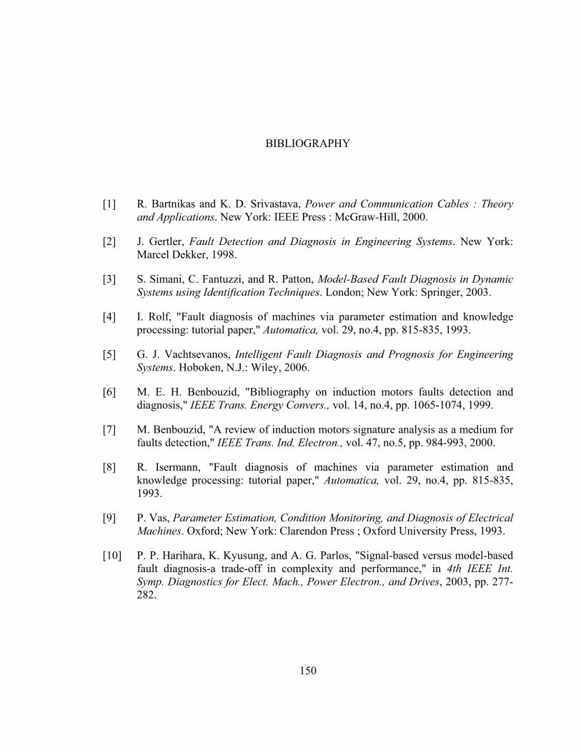
150
BIBLIOGRAPHY
[1] R. Bartnikas and K. D. Srivastava, Power and Communication Cables : Theory and Applications. New York: IEEE Press : McGraw-Hill, 2000.
[2] J. Gertler, Fault Detection and Diagnosis in Engineering Systems. New York: Marcel Dekker, 1998.
[3] S. Simani, C. Fantuzzi, and R. Patton, Model-Based Fault Diagnosis in Dynamic Systems using Identification Techniques. London; New York: Springer, 2003.
[4] I. Rolf, "Fault diagnosis of machines via parameter estimation and knowledge processing: tutorial paper," Automatica, vol. 29, no.4, pp. 815-835, 1993.
[5] G. J. Vachtsevanos, Intelligent Fault Diagnosis and Prognosis for Engineering Systems. Hoboken, N.J.: Wiley, 2006.
[6] M. E. H. Benbouzid, "Bibliography on induction motors faults detection and diagnosis," IEEE Trans. Energy Convers., vol. 14, no.4, pp. 1065-1074, 1999.
[7] M. Benbouzid, "A review of induction motors signature analysis as a medium for faults detection," IEEE Trans. Ind. Electron., vol. 47, no.5, pp. 984-993, 2000.
[8] R. Isermann, "Fault diagnosis of machines via parameter estimation and knowledge processing: tutorial paper," Automatica, vol. 29, no.4, pp. 815-835, 1993.
[9] P. Vas, Parameter Estimation, Condition Monitoring, and Diagnosis of Electrical Machines. Oxford; New York: Clarendon Press ; Oxford University Press, 1993.
[10] P. P. Harihara, K. Kyusung, and A. G. Parlos, "Signal-based versus model-based fault diagnosis-a trade-off in complexity and performance," in 4th IEEE Int. Symp. Diagnostics for Elect. Mach., Power Electron., and Drives, 2003, pp. 277-282.

151
[11] A. Nasiri, J. Poshtan, M. H. Kahaei, and F. Taringoo, "A new scheme in model-based fault detection in three-phase induction motors," in Proc. IEEE Int. Conf. on Mechatronics, 2004, pp. 19-24.
[12] R. Dixon and A. W. Pike, "Application of condition monitoring to an electromechanical actuator: a parameter estimation based approach," Computing & Control Engineering Journal, vol. 13, no.2, pp. 71-81, 2002.
[13] M. A. Awadallah and M. M. Morcos, "Stator-winding fault diagnosis of PM brushless DC motor drives," in Large Eng. Syst. Conf. on Power Eng., 2002, pp. 147-152.
[14] R. Malewski and B. Poulin, "Impulse testing of power transformers using the transfer function method," IEEE Trans. Power Del., vol. 3, no.2, pp. 476-489, 1988.
[15] L. Satish and S. K. Sahoo, "An effort to understand what factors affect the transfer function of a two-winding transformer," IEEE Trans. Power Del., vol. 20, no.2, pp. 1430-1440, 2005.
[16] T. Leibfried and K. Feser, "Monitoring of power transformers using the transfer function method," IEEE Trans. Power Del., vol. 14, no.4, pp. 1333-1341, 1999.
[17] R. Wimmer and K. Feser, "Calculation of the transfer function of a power transformer with online measuring data," in 2nd Int. Conf, on Advances in Processing, Testing, and Application of Dielectric Materials, Wroclaw, Poland 2004.
[18] S. D. Mikkelsen, J. Bak-Jensen, and J. T. Sorensen, "Sensitivity of identified transfer functions in transformer diagnosis," in Proc. Electrical Electronics Insulation Conf. and Electrical Manufacturing & Coil Winding Conf., Chicago, 1993, pp. 533-537.
[19] E. Rahimpour, J. Christian, K. Feser, and H. Mohseni, "Transfer function method to diagnose axial displacement and radial deformation of transformer windings," IEEE Trans. Power Del., vol. 18, no.2, pp. 493-505, 2003.
[20] L. A. Kojovic and C. W. Williams, Jr., "Sub-cycle detection of incipient cable splice faults to prevent cable damage," in IEEE Power Eng. Soc. Summer Meeting, 2000, pp. 1175-1180 vol. 2.
[21] C. Furse, Y. Chung Chung, R. Dangol, M. Nielsen, G. Mabey, and R. Woodward, "Frequency-domain reflectometry for on-board testing of aging aircraft wiring," IEEE Trans. Electromagn. Compat., vol. 45, no.2, pp. 306-315, 2003.

152
[22] C. Furse, P. Smith, M. Safavi, and C. Lo, "Feasibility of spread spectrum sensors for location of arcs on live wires," IEEE Sensors J., vol. 5, no.6, pp. 1445-1450, 2005.
[23] P. Smith, C. Furse, and J. Gunther, "Analysis of spread spectrum time domain reflectometry for wire fault location," IEEE Sensors J., vol. 5, no.6, pp. 1469-1478, 2005.
[24] V. Taylor and M. Faulkner, "Line monitoring and fault location using spread spectrum on power line carrier," IEEE Proc. Generation, Transmission and Distribution, vol. 143, no.5, pp. 427-434, 1996.
[25] P. Tsai, L. Chet, Y. Chung, and C. Furse, "Mixed-signal reflectometer for location of faults on aging wiring," IEEE Sensors J., vol. 5, no.6, pp. 1479-1482, 2005.
[26] S. L. Horton and N. G. Luijk, "Low Voltage Fault Detection and Localisation Using Topas 1000 Disturbance Recorder," Electric Power Quality and Utilization, vol. II, no.1, pp. 27-32, 2006.
[27] C. M. Walton, "Incipient fault detection and management of underground LV networks," in 16th Int. Conf. and Exhibition Electricity Distribution, 2001, p. 5 pp. vol.3.
[28] "IEEE standard for qualifying class 1E electric cables and field splices for nuclear power generating stations," IEEE Standard 383-2003, 2004.
[29] M. Subudhi, "Literature review of environmental qualification of safety-related electric cables: Summary of past work. Volume 1," Nuclear Regulatory Commission, Washington, DC, NUREG/CR-6384-Vol.1, Apr. 1996.
[30] Y. Takezawa, J. Katagiri, and H. Shoji, "Application of optical diagnosis to aged low-voltage cable insulation in nuclear plants," in Conf. on Electrical Insulation and Dielectric Phenomena Annu. Report 2004, pp. 290-293.
[31] C. Cornelissen and A. Schnettler, "Non-destructive diagnostic facilities for cable systems," in Proc. IEEE Int. Symp. on Elect. Insulation, 2002, pp. 557-560.
[32] E. Watanabe, T. Moriya, and M. Yoshizawa, "Ultrasonic visualization method of electrical trees formed in organic insulating materials," IEEE Trans. Dielectr. Electr. Insul., vol. 5, no.5, pp. 767-773, 1998.
[33] Y. Sun, S. Luo, K. Watkins, and C. P. Wong, "Electrical approach to monitor the thermal oxidation aging of carbon black filled ethylene propylene rubber," Polymer Degradation and Stability, vol. 86, no.2, pp. 209-215, 2004.

153
[34] Y. T. Hsu, K. S. Chang-Liao, T. K. Wang, and C. T. Kuo, "Monitoring the moisture-related degradation of ethylene propylene rubber cable by electrical and SEM methods," Polymer Degradation and Stability, vol. 91, no.10, pp. 2357-2364, 2006.
[35] E. A. Vendrusculo and J. A. Pomilio, "Power cable parameters estimation in long distance driving of electrical machines," in Int. Conf. Elect. Mach. and Drives, 1999, pp. 410-412.
[36] N. Ahmed and N. Srinivas, "The noise effect in conducting on-line partial discharge testing in distribution-class cables," in Conf. Elect. Insulation and Dielectric Phenomena Annu. Report, 1998, pp. 319-322 vol. 1.
[37] N. H. Ahmed and N. N. Srinivas, "On-line partial discharge detection in cables," IEEE Trans. Dielectr. Electr. Insul., vol. 5, no.2, pp. 181-188, 1998.
[38] E. Gulski, B. R. Hamerling, F. J. Wester, J. J. Smit, E. A. Groot, and P. Schikarski, "Insulation condition assessment of medium voltage power cables using on-site pd detection and analysis techniques," in 16th Int. Conf. and Exhibition Electricity Distribution, 2001, pp. 84-84.
[39] B. R. Hamerling, F. J. Wester, E. Gulski, J. J. Smit, and E. R. S. Groot, "Fundamental aspects of on-line PD measurements on distribution power cables," in Proc. IEEE 7th Int. Conf. on Solid Dielectrics, 2001, pp. 408-411.
[40] N. Srinivas, N. Ahmed, and G. Raju, "On line measurement of partial discharges," in Conf. on Electrical Insulation and Dielectric Phenomena Annu. Report 2000, pp. 678-681 vol.2.
[41] W. Wang, S. Zhao, B. Cang, and L. En-Heng, "The study of on-line PD detector in power cable," in Proc. 6th Int. Conf. on Properties and Applications of Dielectric Materials, 2000, pp. 177-180 vol.1.
[42] N. Ahmed and N. Srinivas, "On-line versus off-line partial discharge testing in power cables," in Proc. Transmission and Distribution Conf. and Expo., 2001, pp. 865-870 vol.2.
[43] N. Ahmed and N. Srinivas, "Can the operating conditions of the cable system effect the data of the field PD testing?," in Conf. Elect. Insulation and Dielectric Phenomena, 2001, pp. 311-314.
[44] H. E. Orton, "Diagnostic testing of in-situ power cables: an overview," in Transmission and Distribution Conf. and Exhibition, 2002, pp. 1420-1425 vol.2.

154
[45] G. J. Paoletti and A. Golubev, "Partial discharge theory and technologies related to medium-voltage electrical equipment," IEEE Trans. Ind. Appl., vol. 37, no.1, pp. 90-103, 2001.
[46] Q. Su and K. Sack, "New techniques for on-line partial discharge measurements," in Proc. IEEE Int. Multi-Topic Conf., 2001, pp. 49-53.
[47] J. P. Steiner and F. D. Martzloff, "Partial discharges in low-voltage cables," in Conf. Rec. of IEEE Int. Symp. on Electrical Insulation, 1990, pp. 149-152.
[48] W. Pfeiffer, "Partial-discharge testing of components for low-voltage equipment," IEEE Trans. Elect. Insul., vol. 26, no.2, pp. 247-257, 1991.
[49] D. Bogh, J. Coffee, G. Stone, and J. Custodio, "Partial-discharge-inception testing on low-voltage motors," IEEE Trans. Ind. Appl., vol. 42, no.1, pp. 148-154, 2006.
[50] S. Yu, W. Li, B. Zhang, J. He, and Y. Huang, "Analysis of cable parameters on the real chassis by measurement," in 17th Int. Zurich Symp. Electromagnetic Compatibility, 2006, pp. 73-76.
[51] N. Damir, V. Khoi, C. Virgilio, S. Srdjan, and B. Miroslav, "Benefits of synchronized-measurement technology for power-grid applications," in 40th Annual Hawaii Int. Conf. Syst. Sciences, Hawaii, 2007, pp. 118-118.
[52] R. E. Wilson, G. A. Zevenbergen, D. L. Mah, and A. J. Murphy, "Calculation of transmission line parameters from synchronized measurements," Electric Power Components and Systems, vol. 27, no.12, pp. 1269-1278, 1999.
[53] I. Kim and R. K. Aggarwal, "A study on the on-line measurement of transmission line impedances for improved relaying protection," Int. J. Elect. Power & Energy Syst., vol. 28, no.6, p. 359, 2006.
[54] Y. Du and J. Burnett, "Experimental investigation into harmonic impedance of low-voltage cables," IEE Proc. Generation, Transmission and Distribution, vol. 147, no.6, pp. 322-328, 2000.
[55] L. Ljung, System Identification: Theory for the User. Upper Saddle River, NJ: Prentice Hall PTR, 1999.
[56] K. J. Åström and B. Wittenmark, Adaptive Control. Reading, Mass.: Addison-Wesley, 1995.
[57] G. A. Sullivan, "Adaptive control with an expert system based supervisory level," NASA, Washington, DC, NAS 1.26:192742; NASA-CR-192742; RPI-CIRSSE-115, Aug. 1991.
155
[58] B. Porat, "Second-order equivalence of rectangular and exponential windows in least-squares estimation of Gaussian autoregressive processes," IEEE Trans. Acoust., Speech, Signal Process., vol. 33, no.5, pp. 1209-1212, 1985.
[59] T. R. Fortescue, L. S. Kershenbaum, and B. E. Ydstie, "Implementation of self-tuning regulatiors with variable forgetting factors," Automatica, vol. 17, no.6, pp. 831-835, 1981.
[60] M. E. Salgado, G. C. Goodwin, and R. H. Middleton, "Modified least squares algorithm incorporating exponential resetting and forgetting," Int. J. Control, vol. 47, no.2, pp. 477-491, 1988.
[61] T. Hägglund, "Recursive estimation of slowly time-varying parameters," in IFAC Symp. Identification and Sys. Parameter Identification, York, 1985, pp. 1137-1142.
[62] R. Kulhavy, "Restricted exponential forgetting in real-time identification," Automatica, vol. 23, no.5, pp. 589-600, 1987.
[63] S. Bittanti, P. Bolzern, and M. Campi, "Adaptive identification via prediction-error directional forgetting factor: convergence analysis," Int. J. Control, vol. 50, no.6, pp. 2407-2421, 1989.
[64] S. Bittanti, P. Bolzern, and M. Campi, "Convergence and exponential convergence of identification algorithms with directional forgetting factor," Automatica, vol. 26, no.5, pp. 929-932, 1990.
[65] R. Kulhavy and M. B. Zarrop, "On a general concept of forgetting," Int. J. Control, vol. 58, no.4, pp. 905-924, 1993.
[66] J. E. Parkum, N. K. Poulsen, and J. Holst, "Recursive forgetting algorithms," Int. J. Control, vol. 55, no.1, pp. 109-128, 1992.
[67] A. Vahidi, A. Stefanopoulou, and H. Peng, "Recursive least squares with forgetting for online estimation of vehicle mass and road grade: theory and experiments," Vehicle System Dynamics, vol. 43, no.1, pp. 31 - 55, 2005.
[68] L. Cao and H. Schwartz, "A directional forgetting algorithm based on the decomposition of the information matrix," Automatica, vol. 36, pp. 1725-1731, 2000.
[69] L. Cao and H. M. Schwartz, "A decomposition method for positive semidefinite matrices and its application to recursive parameter estimation," SIAM J. on Matrix Analysis and Applications, vol. 22, no.4, pp. 1095-1111, 2001.
156
[70] L. Ljung and T. Söderström, Theory and Practice of Recursive Identification. Cambridge, Mass.: MIT Press, 1983.
[71] G. Avanzolini, P. Barbini, and G. Cevenini, "Two new algorithms for tracking arterial parameters in nonstationary noise conditions," IEEE Trans. Biomed. Eng., vol. 42, no.3, pp. 313-317, 1995.
[72] V. Krishnan, Probability and Random Processes. Hoboken, N.J.: Wiley-Interscience, 2006.
[73] E. Kyriakides and G. T. Heydt, "Calculating confidence intervals in parameter estimation: a case study," IEEE Trans. Power Del., vol. 21, no.1, pp. 508-509, 2006.
[74] J. Fox and G. Monette, "Generalized Collinearity Diagnostics," J. of the American Statistical Association, vol. 87, no.417, pp. 178-183, 1992.
[75] P. M. Anderson, A. A. Fouad, and E. Institute of Electrical and Electronics, Power System Control and Stability. Piscataway, N.J.: IEEE Press; Wiley-Interscience, 2003.
[76] IEEE Standard 399-1997 - IEEE recommended practice for industrial and commercial power systems analysis, 1998
[77] C. A. Gross, Power System Analysis. New York: Wiley, 1986.
[78] ANSI/IEEE Standard 575-1988,IEEE guide for the application of sheath-bonding methods for single-conductor cables and the calculation of induced voltages and currents in cable sheaths, 1987
[79] IEC Standard 60287 - Electric cables - calculation of the current rating, I. E. Commission, 1994
[80] IEEE Standard 1143-1994 - IEEE guide on shielding practice for low voltage cables, 1995
[81] G. J. Anders, Rating of Electric Power Cables : Ampacity Computations for Transmission, Distribution, and Industrial Applications. New York: Institute of Electrical and Electronics Engineers, 1997.
[82] O. I. Gilbertson, Electrical Cables for Power and Signal Transmission. New York: John Wiley, 2000.
[83] IEEE Standard 835-1994 - IEEE Standard Power Cable Ampacity Tables, 1994

157
[84] G. J. Anders, Rating of Electric Power Cables in Unfavorable Thermal Environment. Hoboken, N.J.: Wiley, 2005.
[85] W. A. Thue, Electrical Power Cable Engineering. New York: Marcel Dekker, 1999.
[86] A. B. B. E. S. T. Institute, Electrical Transmission and Distribution Reference Book. Raleigh, N.C.: ABB Electric Systems Technology Institute, 1997.
[87] A. A. Girgis, J. Qiu, and R. B. McManis, "A time-domain approach for distribution and transmission network modeling," IEEE Trans. Power Del., no.1, pp. 365-371, 1990.
[88] A. A. Girgis, W. H. Quaintance, III, J. Qiu, and E. B. Makram, "A time-domain three-phase power system impedance modeling approach for harmonic filter analysis," IEEE Trans. Power Del., vol. 8, no.2, pp. 504-510, 1993.
[89] S. Cobreces, P. Rodriguez, D. Pizarro, F. J. Rodriguez, and E. J. Bueno, "Complex-space recursive least squares power system identification," in IEEE Power Electron. Specialists Conf., 2007, pp. 2478-2484.
[90] P. Zarco and A. G. Exposito, "Power system parameter estimation: a survey," IEEE Trans. Power Syst., vol. 15, no.1, pp. 216-222, 2000.
[91] I. W. Slutsker, S. Mokhtari, and K. A. Clements, "Real time recursive parameter estimation in energy management systems," IEEE Trans. Power Syst., vol. 11, no.3, pp. 1393-1399, 1996.