Improving Multi-class Text Classification with Naive Bayes

by

Jason D. M. Rennie

B.S. Computer ScienceCarnegie Mellon University, 1999

Submitted to the Department of Eleectrical Engineering and Computer Science inPartial Fufillment of the Requirements for the Degree of

Master of Science in Electrical Engineering and Computer Science

at theMassachusetts Institute of Technology

September 2001

c©2001 Massachusetts Institute of Technology. All rights reserved.

Signature of Author . . . . . . . . . . . . . . . . . . . . . . . . . . . . . . . . . . . . . . . . . . . . . . . . . . . . . . . . . . . . . . .Department of Electrical Engineering and Computer Science

September 10, 2001

Certified by: . . . . . . . . . . . . . . . . . . . . . . . . . . . . . . . . . . . . . . . . . . . . . . . . . . . . . . . . . . . . . . . . . . . . . . .Tommi Jaakkola

Assistant Professor of Electrical Engineering and Computer ScienceThesis Supervisor

Accepted by: . . . . . . . . . . . . . . . . . . . . . . . . . . . . . . . . . . . . . . . . . . . . . . . . . . . . . . . . . . . . . . . . . . . . . .Arthur C. Smith

Chairman, Committee on Graduate StudentsDepartment of Electrical Engineering and Computer Science

Improving Multi-class Text Classificationwith Naive Bayes

byJason D. M. Rennie

Submitted to the Department of Electrical Engineering and Computer Scienceon September 10, 2001, in partial fulfillment of the

requirements for the degree ofMaster of Science

Abstract

There are numerous text documents available in electronic form. More and moreare becoming available every day. Such documents represent a massive amount ofinformation that is easily accessible. Seeking value in this huge collection requiresorganization; much of the work of organizing documents can be automated throughtext classification. The accuracy and our understanding of such systems greatlyinfluences their usefulness. In this paper, we seek 1) to advance the understandingof commonly used text classification techniques, and 2) through that understanding,improve the tools that are available for text classification. We begin by clarifyingthe assumptions made in the derivation of Naive Bayes, noting basic properties andproposing ways for its extension and improvement. Next, we investigate the qualityof Naive Bayes parameter estimates and their impact on classification. Our analysisleads to a theorem which gives an explanation for the improvements that can befound in multiclass classification with Naive Bayes using Error-Correcting OutputCodes. We use experimental evidence on two commonly-used data sets to exhibit anapplication of the theorem. Finally, we show fundamental flaws in a commonly-usedfeature selection algorithm and develop a statistics-based framework for text featureselection. Greater understanding of Naive Bayes and the properties of text allows usto make better use of it in text classification.

Thesis Supervisor: Tommi JaakkolaTitle: Assistant Professor of Electrical Engineering and Computer Science

2

Contents

1 Introduction 7

2 Naive Bayes 92.1 ML Naive Bayes . . . . . . . . . . . . . . . . . . . . . . . . . . . . . . 92.2 MAP Naive Bayes . . . . . . . . . . . . . . . . . . . . . . . . . . . . . 112.3 Expected Naive Bayes . . . . . . . . . . . . . . . . . . . . . . . . . . 122.4 Bayesian Naive Bayes . . . . . . . . . . . . . . . . . . . . . . . . . . . 122.5 Bayesian Naive Bayes Performs Worse In Practice . . . . . . . . . . . 132.6 Naive Bayes is a Linear Classifier . . . . . . . . . . . . . . . . . . . . 152.7 Naive Bayes Outputs Are Often Overconfident . . . . . . . . . . . . . 16

3 Analysis of Naive Bayes Parameter Estimates 183.1 Consistency . . . . . . . . . . . . . . . . . . . . . . . . . . . . . . . . 183.2 Bias . . . . . . . . . . . . . . . . . . . . . . . . . . . . . . . . . . . . 193.3 Variance . . . . . . . . . . . . . . . . . . . . . . . . . . . . . . . . . . 193.4 The Danger of Imbalanced Class Training Data . . . . . . . . . . . . 22

4 Error-correcting Output Coding 244.1 Introduction . . . . . . . . . . . . . . . . . . . . . . . . . . . . . . . . 244.2 Additive Models . . . . . . . . . . . . . . . . . . . . . . . . . . . . . . 25

4.2.1 The relation to boosting . . . . . . . . . . . . . . . . . . . . . 254.3 The Support Vector Machine . . . . . . . . . . . . . . . . . . . . . . . 264.4 Experiments . . . . . . . . . . . . . . . . . . . . . . . . . . . . . . . . 26

4.4.1 The success and failure of Naive Bayes . . . . . . . . . . . . . 284.4.2 Multiclass error is a function of binary performance . . . . . . 294.4.3 Non-linear loss does not affect ECOC performance . . . . . . . 33

5 Feature Selection 345.1 Information Gain . . . . . . . . . . . . . . . . . . . . . . . . . . . . . 345.2 Hypothesis Testing . . . . . . . . . . . . . . . . . . . . . . . . . . . . 355.3 The Generalization Advantage of Significance Level . . . . . . . . . . 355.4 The Undesirable Properties of IG and HT . . . . . . . . . . . . . . . 365.5 Simple Discriminative Feature Selection . . . . . . . . . . . . . . . . . 365.6 A New Feature Selection Framework . . . . . . . . . . . . . . . . . . 37

3

6 Conclusion 39

A Data Sets 40

4

List of Figures

2-1 The document generation model . . . . . . . . . . . . . . . . . . . . . 10

3-1 The distribution and variance of log(1 +Nk) . . . . . . . . . . . . . . 203-2 Classification output variance . . . . . . . . . . . . . . . . . . . . . . 21

4-1 A comparison of multiclass classification schemes . . . . . . . . . . . 284-2 Binary error is a poor indicator of multiclass performance . . . . . . . 294-3 Multiclass vs. binary performance . . . . . . . . . . . . . . . . . . . . 304-4 One-vs-all multiclass error vs. ROC breakeven . . . . . . . . . . . . . 31

5-1 A new statistics-based framework for feature selection . . . . . . . . . 37

5

List of Tables

2.1 Bayesian Naive Bayes classification results . . . . . . . . . . . . . . . 142.2 Maximum term frequency for Bayesian and MAP Naive Bayes . . . . 142.3 MAP Naive Bayes produces overconfident posteriors . . . . . . . . . . 16

3.1 20 Newsgroup words with high log-odds ratio . . . . . . . . . . . . . 22

4.1 ECOC multiclass performance . . . . . . . . . . . . . . . . . . . . . . 274.2 Binary confusion matrix . . . . . . . . . . . . . . . . . . . . . . . . . 294.3 ECOC binary performance . . . . . . . . . . . . . . . . . . . . . . . . 324.4 Linear loss function is as effective as hinge . . . . . . . . . . . . . . . 32

6

Chapter 1

Introduction

There are numerous text documents available in electronic form. More are becomingavailable constantly. The Web itself contains over a billion documents. Millionsof people send e-mail every day. Academic publications and journals are becomingavailable in electronic form. These collections and many others represent a massiveamount of information that is easily accessible. However, seeking value in this hugecollection requires organization. Many web sites offer a hierarchically-organized viewof the Web. E-mail clients offer a system for filtering e-mail. Academic communitiesoften have a Web site that allows searching on papers and shows an organizationof papers. However, organizing documents by hand or creating rules for filtering ispainstaking and labor-intensive. This can be greatly aided by automated classifiersystems. The accuracy and our understanding of such systems greatly influencestheir usefulness. We aim 1) to advance the understanding of commonly used textclassification techniques, and 2) through that understanding, to improve upon thetools that are available for text classification.

Naive Bayes is the de-facto standard text classifier. It is commonly used in practiceand is a focus of research in text classification. Chakrabarti et al. use Naive Bayesfor organizing documents into a hierarchy for better navigation and understandingof what a text corpus has to offer [1997]. Frietag and McCallum use a Naive Bayes-like model to estimate the word distribution of each node of an HMM to extractinformation from documents [1999]. Dumais et al. use Naive Bayes and other textclassifiers to automate the process of text classification [1998]. That Naive Bayes isso commonly used is an important reason to gain a better understanding of it. NaiveBayes is a tool that works well in particular cases, but it is important to be ableto identify when it is effective and when other techniques are more appropriate. Athorough understanding of Naive Bayes also makes it easier to extend Naive Bayesand/or tune it to a particular application.

There has been much work on Naive Bayes and text classification. Lewis givesa review of the use of Naive Bayes in information retrieval [Lewis, 1998]. Unliketext classification, information retrieval practitioners usually assume independencebetween features and ignore word frequency and document-length information. Themultinomial model used for text classification is different and must be treated assuch. Domingos and Pazzani discuss conditions for when Naive Bayes is optimal

7

for classification even when its probability assessments are incorrect [Domingos andPazzani, 1996]. Domingos and Pazzani clarify this point and show simple cases ofwhen Naive Bayes is optimal for classification. Analysis of Naive Bayes like thework of Domingos and Pazzani is important, but little such work exists. Bergerand Ghani individually ran experiments using ECOC with Naive Bayes. Both foundthat they were able to improve performance over regular Naive Bayes [Berger, 1999;Ghani, 2000]. But, neither adequately explains why regular Naive Bayes performspoorly compared to ECOC. Yang and Pedersen conduct an empirical study of featureselection methods for text classification [Yang and Pedersen, 1997]. They give anevaluation of five different feature selection techniques and provide some analysis oftheir differences. But, there is still need for better understanding of what makesa good feature selection method. Yang and Pedersen say that common terms areinformative for text classification, but there are certainly other factors at work.

The application of Naive Bayes to multiclass text classification is still not wellunderstood. An important factor affecting the performance of Naive Bayes is thequality of the parameter estimates. Text is special since there is a large numberof features (usually 10,000 or more) and many features that provide informationfor classification will occur only a handful of times. Also, poor estimates due toinsufficient examples in one class can affect the classifier as a whole. We approachthis problem by analyzing the bias and variance of Naive Bayes parameter estimates.

Naive Bayes is suited to perform multiclass text classification, but there is reasonto believe that other schemes (such as ECOC and multiclass boosting) can yieldimproved performance using Naive Bayes as a component. Regular Naive Bayes canbe more efficient than these schemes, so it is important to understand when theyimprove performance and when they merely add inefficient baggage to the multiclasssystem. We show how ECOC can yield improved performance over regular NaiveBayes and give experimental evidence to back our claims.

The multitude of words that can be found in English (and other languages) oftendrives practitioners to reduce their number through feature selection. Feature selec-tion can also improve generalization error by eliminating features with poor parameterestimates. But, the interaction between feature selection algorithms and Naive Bayesis not well understood. Also, commonly used algorithms have properties that are notappropriate for multiclass text classification. We point out these flaws and suggest anew framework for text feature selection.

8

Chapter 2

Naive Bayes

When someone says “Naive Bayes,” it is not always clear what is meant. McCallumand Nigam clarify the picture by defining two different Naive Bayes “event models”and provide empirical evidence that the multinomial event model should be preferredfor text classification [1998]. But, there are multiple methods for obtaining the pa-rameter estimates. In the interest of clarity, we carefully step through the multinomialderivation of Naive Bayes and distinguish between variations within that model. Wealso present a fully Bayesian derivation of Naive Bayes, that, while not new, has yet tobe advertised as an algorithm for text classification. Through a careful presentation,we hope to clarify the basis of Naive Bayes and to give insight into how it can beextended and improved.

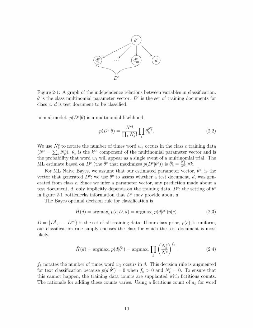
To simplify our work, we assume that for each class, c ∈ {1, . . . ,m}, there is an(unknown) parameter vector, θc, which generates documents independently. Somedocuments are observed as being part of a particular class (known as training docu-ments and designated with Dc); others are test documents. This model is depicted infigure 2-1. We further assume that the generation model is a multinomial and ignoredocument length concerns.

2.1 ML Naive Bayes

One formulation of Naive Bayes is to choose the parameters that produce the largestlikelihood for the training data. One then makes predictions using the estimatedparameter vector, θc. This method has obvious flaws and includes strong assumptionsabout the generation of data. For example, any feature that does not occur in thetraining data for a class is assumed to not occur in any document generated by thatclass. However, this method, known as Maximum Likelihood (ML) can be effectivein practice and is efficient to implement. It is used regularly in other domains. Wecall the multinomial version of this ML Naive Bayes.

The ML parameter for class c is

θc = argmaxθ p(Dc|θ). (2.1)

Dc is the training data for class c and θc is the class c parameter vector for a multi-

9

ONMLHIJKθc

wwpppppppppppppppp

�����������

�� ��????????

GFED@ABCdc1 · · · ONMLHIJKdcm GFED@ABCd

Dc

Figure 2-1: A graph of the independence relations between variables in classification.θ is the class multinomial parameter vector. Dc is the set of training documents forclass c. d is test document to be classified.

nomial model. p(Dc|θ) is a multinomial likelihood,

p(Dc|θ) =N c!∏kN

ck !

∏k

θNck

k . (2.2)

We use N ck to notate the number of times word wk occurs in the class c training data

(N c =∑

kNck). θk is the kth component of the multinomial parameter vector and is

the probability that word wk will appear as a single event of a multinomial trial. TheML estimate based on Dc (the θc that maximizes p(Dc|θc)) is θck =

Nck

Nc ∀k.

For ML Naive Bayes, we assume that our estimated parameter vector, θc, is thevector that generated Dc; we use θc to assess whether a test document, d, was gen-erated from class c. Since we infer a parameter vector, any prediction made about atest document, d, only implicitly depends on the training data, Dc; the setting of θc

in figure 2-1 bottlenecks information that Dc may provide about d.The Bayes optimal decision rule for classification is

H(d) = argmaxc p(c|D, d) = argmaxc p(d|θc)p(c). (2.3)

D = {D1, . . . , Dm} is the set of all training data. If our class prior, p(c), is uniform,our classification rule simply chooses the class for which the test document is mostlikely,

H(d) = argmaxc p(d|θc) = argmaxc∏k

(N ck

N c

)fk. (2.4)

fk notates the number of times word wk occurs in d. This decision rule is augmentedfor text classification because p(d|θc) = 0 when fk > 0 and N c

k = 0. To ensure thatthis cannot happen, the training data counts are supplanted with fictitious counts.The rationale for adding these counts varies. Using a fictitious count of ak for word

10

wk (a =∑

k ak), we arrive at the modified decision rule,

H(d) = argmaxc∏k

(N ck + akN c + a

)fk. (2.5)

Uniform fictitious counts (ai = aj ∀i, j) across all words are often used. A commonchoice is ak = 1.

2.2 MAP Naive Bayes

ML Naive Bayes leaves something to be desired because it does not include the frame-work to explain the fictitious counts. As a result, we do not know what the fictitiouscounts represent. We would like to know what assumptions about parameter estima-tion underpins their inclusion in the decision rule. For this, we turn to a generaliza-tion of ML estimation, Maximum A Posteriori (MAP) estimation. MAP estimationproduces the “fictitious counts” thorough a particular choice of parameter prior dis-tribution. Except for the change in the way we estimate parameters, MAP NaiveBayes is identical to ML Naive Bayes. We still select a “best” parameter vector, θc

and use that vector for classification.For MAP estimation, we estimate the parameter vector according to

θc = argmaxθ p(θ|Dc) = argmaxθ p(Dc|θ)p(θ), (2.6)

where p(θ) is the parameter prior term. MAP estimation is a generalization of MLestimation; ML is MAP with p(θ) = C (C is the appropriate constant). We choosethe Dirichlet as the general form of the prior. It has hyper-parameters{αk}, αk > 0(α =

∑k αk). The density of the Dirichlet is

p(θ) = Dir(θ|{αk}) =Γ(α)∏k Γ(αk)

∏k

θαk−1k . (2.7)

Γ(x) is the Gamma function. It satisfies Γ(x+1) = xΓ(x) and Γ(1) = 1. Γ(n+1) = n!for n ∈ {0, 1, 2, . . . }. A valuable property of the Dirichlet is that it is the the conjugateprior to the multinomial distribution. This makes the posterior distribution Dirichlet,

p(θ|Dc) =p(Dc|θ)p(θ)p(Dc)

= Dir(θ|{N ck + αk}). (2.8)

Setting θk =Nck+αk−1

Nc+α−V maximizes this expression (for αk ≥ 1). V is the size of thevocabulary. Setting αk = ak + 1 gives us the “fictitious counts” in equation 2.5without any ad hoc reasoning. The MAP derivation makes clear that the fictitiouscounts represent a particular prior distribution on the parameter space. In particular,the common choice of ak = 1 ∀i represents a prior distribution in which more uniformparameters (e.g. θk = 1

V∀i) are preferred.

11

2.3 Expected Naive Bayes

The MAP NB decision rule is commonly used, but it is sometimes derived in a differentway [Chakrabarti et al., 1997] [Ristad, 1995]. Instead of maximizing some aspect ofthe data, an expected value of the parameter is used,

θck = E[θck|N ck ] =

∫θp(θ|N c

k)dθ =

∫θp(N c

k |θ)p(θ)p(N c

k)dθ. (2.9)

θck is the estimate of the parameter θck. Nck is the number of times word wk appears

in class c training documents. With a uniform prior, we get the MAP NB decisionrule with ak = 1 ∀k,

E[θck|N ck ] =

N ck + 1

N c + V. (2.10)

V is the size of the vocabulary. Maximizing the posterior with a prior that prefersuniform parameters (αk = 2 ∀k) gives us the same parameter estimates as when auniform prior and expected values are used.

2.4 Bayesian Naive Bayes

MAP Naive Bayes chooses a particular parameter vector, θc, for classification. Thissimplifies the derivation, but bottlenecks information about the training data forclassification. An alternative approach is to use a distribution of parameters based onthe data. This complicates the derivation somewhat since we don’t evaluate p(d|c,D)as p(d|θc). Instead, we integrate over all possible parameters, using p(θ|Dc) as ourbelief that a particular set of parameters generated Dc.

As in ML & MAP Naive Bayes, we start with the Bayes optimal decision rule,

H(d) = argmaxc p(c|D, d) = argmaxc p(d|c,D)p(c). (2.11)

We expand p(d|c,D) to

p(d|c,D) =

∫p(d|θ)p(θ|Dc)dθ. (2.12)

p(d|θ) = f !∏k fk!

∏k θ

fkk is the multinomial likelihood. We expand the posterior via

Bayes’ Law, p(θ|Dc) = p(Dc|θ)p(θ)p(Dc)

and use the Dirichlet prior, as we did with MAPNaive Bayes. This gives us a Dirichlet posterior,

p(θ|Dc) = Dir(θ|{αi +N ci }) =

Γ(α +N c)∏i Γ(αi +N c

i )

∏i

θNci +αi−1

i . (2.13)

12

Substituting this into equation 2.11 and selecting p(c) = 1m

, we get

H(d) = argmaxcΓ(α +N c)∏i Γ(αi +N c

i )

∏i Γ(N c

i + αi + fi)

Γ(N c + α + f). (2.14)

This fully Bayesian derivation is distinct from the MAP and ML derivations, butit shares similarities. In particular, if we make the approximations

Γ(α +N c)

Γ(α +N c + f)≈ 1

(α +N c)fand

∏i Γ(αi +N c

i + fi)∏i Γ(αi +N c

i )≈∏i

(αi +N ci )fi , (2.15)

we get a decision rule very similar to that of MAP Naive Bayes,

H(d) = argmaxc∈C∏k

(αk +N c

k

α +N c

)fk. (2.16)

The lone difference is that MAP Naive Bayes uses different Dirichlet hyper-parametersto achieve this rule.

Bayesian Naive Bayes is distinct from MAP Naive Bayes in its decision rule.As shown above, modifications can be made to make the two identical, but thosemodifications are not generally appropriate. In fact, the modifications exhibit thedifferences between MAP and Bayesian Naive Bayes. Compared to MAP, BayesianNaive Bayes over-emphasizes words that appear more than once in a test document.Consider binary (+1,−1) classification with N+1 = N−1. Let d be a test documentin which the word wk appears twice. The contribution for wk in MAP Naive Bayes is(ak +N c

k)2; the similar contribution for wk in Bayesian Naive Bayes is (αk +N c

k)(αk +N ck + 1). The Bayesian term is larger even though other terms are identical. The

difference is greater for a word that occurs more frequently.

2.5 Bayesian Naive Bayes Performs Worse In Prac-

tice

On one of the two data sets that we tried, we found that Bayesian NB (with a Dirichletprior and αk = 1 ∀k) performed worse than MAP NB (using a Dirichlet prior andαk = 2 ∀k). This is not a sign that the Bayesian derivation is bad—far from it.The poor empirical performance is rather an indication that the Dirichlet prior is apoor choice or that the Dirichlet hyper-parameter settings are not well chosen. Wellestimated hyper-parameters, or a different prior, such as the Dirichlet process, mayyield better performance for Bayesian NB [Ferguson, 1973]. We show the empiricaldifference and give statistics exhibiting the conditions where classification differencesoccur.

We conducted classification experiments on the 20 Newsgroups and Industry Sec-tor data sets. Table 2.1 shows empirical test error averaged over 10 test/train splits.See appendix A for a full description of the data sets and the preparations used for

13

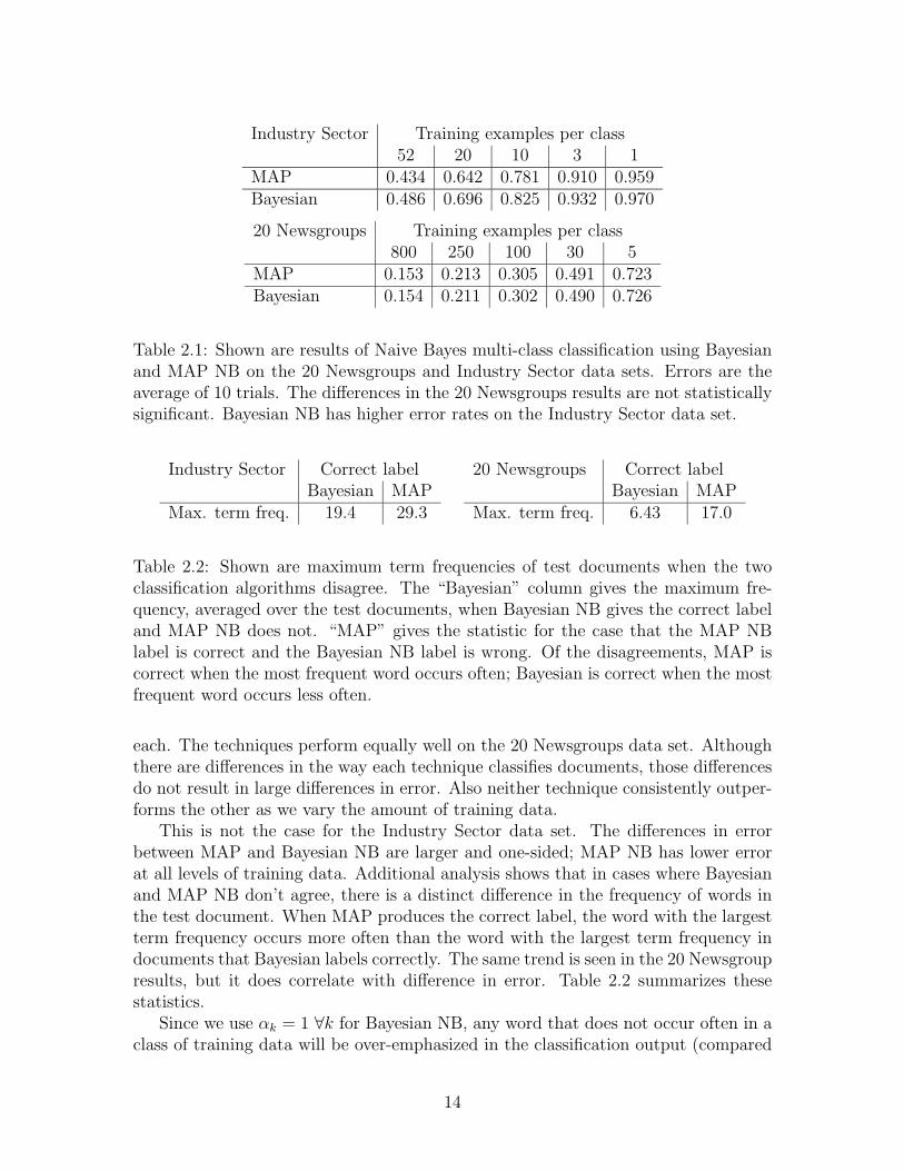
Industry Sector Training examples per class52 20 10 3 1

MAP 0.434 0.642 0.781 0.910 0.959Bayesian 0.486 0.696 0.825 0.932 0.970

20 Newsgroups Training examples per class800 250 100 30 5

MAP 0.153 0.213 0.305 0.491 0.723Bayesian 0.154 0.211 0.302 0.490 0.726

Table 2.1: Shown are results of Naive Bayes multi-class classification using Bayesianand MAP NB on the 20 Newsgroups and Industry Sector data sets. Errors are theaverage of 10 trials. The differences in the 20 Newsgroups results are not statisticallysignificant. Bayesian NB has higher error rates on the Industry Sector data set.

Industry Sector Correct labelBayesian MAP

Max. term freq. 19.4 29.3

20 Newsgroups Correct labelBayesian MAP

Max. term freq. 6.43 17.0

Table 2.2: Shown are maximum term frequencies of test documents when the twoclassification algorithms disagree. The “Bayesian” column gives the maximum fre-quency, averaged over the test documents, when Bayesian NB gives the correct labeland MAP NB does not. “MAP” gives the statistic for the case that the MAP NBlabel is correct and the Bayesian NB label is wrong. Of the disagreements, MAP iscorrect when the most frequent word occurs often; Bayesian is correct when the mostfrequent word occurs less often.

each. The techniques perform equally well on the 20 Newsgroups data set. Althoughthere are differences in the way each technique classifies documents, those differencesdo not result in large differences in error. Also neither technique consistently outper-forms the other as we vary the amount of training data.

This is not the case for the Industry Sector data set. The differences in errorbetween MAP and Bayesian NB are larger and one-sided; MAP NB has lower errorat all levels of training data. Additional analysis shows that in cases where Bayesianand MAP NB don’t agree, there is a distinct difference in the frequency of words inthe test document. When MAP produces the correct label, the word with the largestterm frequency occurs more often than the word with the largest term frequency indocuments that Bayesian labels correctly. The same trend is seen in the 20 Newsgroupresults, but it does correlate with difference in error. Table 2.2 summarizes thesestatistics.

Since we use αk = 1 ∀k for Bayesian NB, any word that does not occur often in aclass of training data will be over-emphasized in the classification output (compared

14

to MAP NB). But, our choice of {αk} corresponds to a prior. αk = 1 corresponds toa preference for uniform parameter vectors—vectors where all words have the sameprobability. This isn’t a reasonable prior for English or other languages. A moreappropriate prior would cause only novel words to be over-emphasized.

The poor performance by Bayesian NB is not a fault of the classification algorithm,but rather a sign that our choice of prior or model is poor. The Bayesian derivationprovides us with a classification rule that directly incorporates information from thetraining data and may be more sensitive to our choice of prior. Future work to betterour choice of model and prior should improve the performance of Bayesian NB.

2.6 Naive Bayes is a Linear Classifier

MAP Naive Bayes is known to be a linear classifier. In the case of two classes, +1and −1, the classification output is

h(d) = logp(d|θ+1)p(+1)

p(d|θ−1)p(−1)(2.17)

= logp(+1)

p(−1)+∑k

fk

(log

ak +N+1k

a+N+1− log

ak +N−1k

a+N−1

)= b+

∑k

wkfk, (2.18)

where h(d) > 0 corresponds to a +1 classification and h(d) < 0 corresponds to a−1 classification. We use wk to represent the linear weight for the kth word in thevocabulary. This is identical in manner to the way in which logistic regression andlinear SVMs score documents. Logistic regression classifies according to

p(y = +1|x,w) = g(b+∑k

wkxk), (2.19)

where p(y = +1|x,w) > 0.5 is a +1 classification and p(y = +1|x,w) < 0.5 is a −1classification. g(z) = (1 + exp(−z))−1. Similarly, the linear SVM classifies accordingto h(x) = b +

∑k wkxk, assigning class +1 for h(x) > 0 and class −1 for h(x) < 0.

Hence, all three algorithms are operationally identical in terms of how they classifydocuments. The only difference is in the way in which their weights are trained.

This similarity extends to multi-class linear classifiers. Softmax is the standardextension of logistic regression to the linear case. Given a multi-class problem withclasses {1, . . . ,m}, Softmax computes

zi = bi +∑k

wikxk (2.20)

for each class and assigns probabilities p(y = i|x,w) = exp(zi)∑j exp(zj)

. The class with

the largest zi and hence the largest probability is declared the label for example x.

15

(a)

percentile min. posterior0% 0.0501211% 0.9648622% 0.9998733% 1.0000044% 1.0000055% 1.0000066% 1.0000077% 1.0000088% 1.0000099% 1.00000

(b)

percentile # digits11% 116% 220% 324% 428% 531% 635% 738% 840% 9

Table 2.3: Shown are maxcp(c|D, d) values produced by MAP Naive Bayes on 20Newsgroup data. (a) shows the smallest value at each of 11 percentile levels. NaiveBayes produced a value of 1 on a majority of the test data. (b) shows the percentileat which rounding any posterior to the given number of digits would produce a valueof 1. The posteriors tend to 1 rapidly.

Similarly the MAP Naive Bayes decision rule is

H(d) = argmaxi p(d|θci) (2.21)

= argmaxi∑k

log p(ci) + fk logak +N i

k

a+N i= argmaxi

(bi +

∑k

wikfk

). (2.22)

Hence, Naive Bayes and Softmax are operationally identical. The extension of thelinear SVM to multi-class also shares this form. The only distinction between thesealgorithms is in the way their weights are trained.

2.7 Naive Bayes Outputs Are Often Overconfident

Consider a pair of unfair coins. Each comes up heads 60% of the time. When wecount only the times that both coins show the same side, heads appears 69% of thetime. Coins which marginally show heads 90% of the time are heads 99% of the timewhen both coins show the same side. Consider casting a spell over our 90% headscoins so that the second coin always lands on the same side as the first. If we nowmodel the two coins as being independent and observe a large number of flips, wewould estimate that when both coins land on the same side, heads shows 99% of thetime. In fact, the probability of such an event is only 90%. The same effect occurs inMAP Naive Bayes.

It is rare that words serve as exact duplicates of each other, such as in our coinexample. However, distinguishing between 20 classes requires a mere 2 word vocab-ulary and 5 terms per document for correct classification; all remaining information

16

about the class variable is either noisy or redundant. Text databases frequently have10,000 to 100,000 distinct vocabulary words; documents often contain 100 or moreterms. Hence, there is great opportunity for duplication.

To get a sense of how much duplication there is, we trained a MAP Naive Bayesmodel with 80% of the 20 Newsgroups documents. We produced p(c|d,D) (posterior)values on the remaining 20% of the data and show statistics on maxc p(c|d,D) intable 2.3. The values are highly overconfident. 60% of the test documents are assigneda posterior of 1 when rounded to 9 decimal digits. Unlike logistic regression, NaiveBayes is not optimized to produce reasonable probability values. Logistic regressionperforms joint optimization of the linear coefficients, converging to the appropriateprobability values with sufficient training data. Naive Bayes optimizes the coefficientsone-by-one. It produces realistic outputs only when the independence assumptionholds true. When the features include significant duplicate information (as is usuallythe case with text), the posteriors provided by Naive Bayes are highly overconfident.

17

Chapter 3

Analysis of Naive Bayes ParameterEstimates

Having an understanding of how MAP Naive Bayes parameter estimates affect clas-sification is important. The quality of the parameter estimates directly affects per-formance. We show that Naive Bayes estimates are consistent; we then investigatetheir behavior for finite training data by analyzing their bias and variance. The biasin the estimate is a direct product of the prior and tends monotonically toward zerowith more training data. The variance peaks when a word is expected to occur 1-2times in the training data and falls off thereafter. This analysis shows that insufficienttraining examples in one class can negatively affect overall performance. The varianceas a whole is the sum of the variances of the individual components. If a single classvariance is large, the overall variance is also high.

3.1 Consistency

MAP Naive Bayes estimates a vector of parameters, θc for the multinomial model.Each individual parameter, θck, is the estimated probability of word wk appearing in aparticular position of a class c document. Let {αk} be the parameters of the Dirichletprior (α =

∑k αk), ak = αk−1 (a =

∑k ak) and let N c

k be the number of occurrencesof word wk in the training documents (N c =

∑kN

ck). Then the MAP estimate for

wk is

θck =ak +N c

k

a+N c. (3.1)

A basic desirable property of parameter estimates is consistency, or the conver-gence of the estimates to the true values when the amount of data used to make theestimates grows large. Cover and Thomas describe the method of types as a way todescribe properties of empirical distributions [Cover and Thomas, 1991]. Let X be amultinomial random variable with parameters {θck}. Let pX represent the distributionof the parameters. Let pY represent the empirical distribution when N c samples aretaken from X resulting in counts of {N c

k}. Then, our MAP estimates are θck =ak+Nc

k

a+Nc .

18

The probability of observing such counts and hence the probability of making suchestimates is

p(θc|θc) =N c!∏kN

ck !

∏k

(θck)Nk =

N c!∏kN

ck !

2−N(H(pY )+D(pY ||pX)), (3.2)

The mean of our estimate is

θck =ak +N cθcka+N c

, (3.3)

which goes to θck as N c →∞. The variance of our estimate is

σ2c,k =

N cθk(1− θck)(a+N c)2

, (3.4)

which goes to zero as N c → ∞. Hence, MAP estimates are consistent; in the limit,they are unbiased and have zero variance. So, as the size of the observed data growslarge, our estimates converge to the true parameters.

3.2 Bias

Since we never have infinite training data in practice, it is more important to under-stand the behavior of estimates for finite training data. For a particular number ofobserved words, N c, the bias in the estimate for word wk is

bias(θck) =ak +N cθcka+N c

− θck =ak − aθcka+N c

(3.5)

Hence, for words where θck >aka

, the expected estimate is smaller and for θck <aka

, theexpected estimate is larger than the true value. This is a natural consequence of thechoice of a Dirichlet prior. Also, bias lessens as the amount of training data growslarge.

3.3 Variance

The variance of a parameter estimate yields little insight into the effect estimateshave on classification. Since Naive Bayes is a linear classifier, a more useful variancequantity to examine is the variance of each individual term in the classification output.Let fk be the frequency of word k in the test document (f =

∑k fk). Then

zc = −f log(a+N c) +∑k

fk log(ak +N ck) (3.6)

is the classification score for class c. The assigned class is the one with the largestscore. The individual terms of the sum are independent (assuming N c to not be

19

a)

0

0.05

0.1

0.15

0.2

0.25

0.3

0 0.5 1 1.5 2 2.5 3

Pro

babi

lity

mas

s

log(1+N_k)

b)

0

0.05

0.1

0.15

0.2

0.25

0.3

100 1000 10000 100000 1e+06

Var

(log(

1+N

_k))

N

Figure 3-1: (a) is a plot of the pmf of log(1 +Nk) for θck = 0.0002 where N = 10000.(b) plots the variance of log(1 + Nk) for θck = 0.0002 as we vary N . Note the x-axislog scale. var(log(1 + Nk)) peaks when the word is expected to occur 1-2 times. (b)is representative of all θcks. The plot of var(log(1 +Nk)) peaks near θck = 1/N and hasthe same shape as the one shown.

fixed), so

var(zi) =∑k

f 2kvar(log(ak +N i

k)). (3.7)

We assume the {fk} to be fixed and that the {N ck} may vary. The variance of an

individual term is

var(log(ak +N ik)) = E[(log(ak +N i

k)2]− E[log(ak +N i

k)]2. (3.8)

Treating each Nk as a binomial with parameter θck, we get

E[log(ak +N ik)] =

∑n

log(ak + n)

(N

n

)(θck)

n (1− θck)(N−n). (3.9)

Although equation 3.9 is not difficult to compute, we approximate Nk as a Poissonwith λ = θck and use Stirling’s formula for n! to arrive at

E[log(ak +N ik)] =

Nθck log(2)

exp(Nθck)+

N∑n=2

log(ak + n)√2πn

exp(n(1 + log(Nθck)− log n)−Nθck).

(3.10)

We use this formula for the graphs that we present. The Poisson approximation isgood for θck << 1, which is generally the case in text.

Figure 3-1 shows plots of the the pmf and variance for a word with θck = 0.0002.var(log(1 +Nk)) is maximized when wk is expected to occur 1-2 times in the trainingdata. This does not incorporate fk; a word that occurs 1-2 times in the training data

20

0

0.0005

0.001

0.0015

0.002

0.0025

0.003

1e-06 1e-05 0.0001 0.001 0.01 0.1

f_k

var(

log(

1+N

_k))

\theta

Figure 3-2: Shown is the per-word variance contribution to the classification outputfor N = 1000000, f = 300 and various values of θck . We assume that fk = fθck.Although var(log(1 +Nk)) is largest for θck = 0.000001, larger values of θck yield largerper-word variance contributions.

for class c is unlikely to occur in test documents generated from class c. However,figure 3-1 does give us the ability to compare variances across classes. Let θ+1

k = 0.02and θ−1

k = 0.0002 be the true parameters for wk for the classes +1 and −1. If thetraining data for both classes consists of 10,000 words, N+1 = N−1 = 10, 000 thenthe wk contribution to the variance of the classification output will be much greaterfor class −1 than for class +1.

Figure 3-2 shows the variance contribution of individual tokens assuming thatfk = fθck. Words with the largest θck contribute the largest variance to the classifi-cation output. fk ≈ fθck is only reasonable for class-independent words and for testdocuments drawn from class c. Words with large θck values often contribute the great-est amount of variance to classification outputs, but, a word with small θck can easilycontribute a great deal of variance if wk occurs frequently in the test document.

We can glean from figure 3-1 the effect of additional training data on classification.It is widely believed that additional training data improves classification. The plotof the variance of log(1 +Nk) shows that for every word, there is a point after whichthe variance contribution for that word diminishes with additional training data.Once that point is passed for most words, the overall variance in the classificationoutput decreases monotonically. Before this point, output variance may increase withadditional training data, but when the amount of training data is relatively small, biasis a significant factor. For N = 1000 and a word with θck = 0.00002, the estimate may

be θck = 0.0001, five times the actual parameter value. When the amount of trainingdata is very small, bias plays a greater role in affecting classification performance.Our analysis of variance shows that after a point variance decreases monotonicallyfor each word. This lessening of variance contributes to improved classification as thenumber of training examples increases.

21

category word log-odds ratio θkalt.atheism atheism 0.013 0.0040comp.graphics jpeg 0.037 0.0073comp.os.ms-windows.misc windows 0.043 0.020comp.sys.ibm.pc.hardware scsi 0.033 0.012comp.sys.mac.hardware mac 0.024 0.012comp.windows.x window 0.024 0.0091misc.forsale sale 0.018 0.0076rec.autos car 0.043 0.017rec.motorcycles bike 0.045 0.010rec.sport.baseball baseball 0.016 0.0057rec.sport.hockey hockey 0.037 0.0078sci.crypt clipper 0.033 0.0058sci.electronics circuit 0.010 0.0031sci.med patients 0.011 0.0029sci.space space 0.035 0.013soc.religion.christian god 0.035 0.018talk.politics.guns gun 0.028 0.0094talk.politics.mideast armenian 0.039 0.0057talk.politics.misc stephanopoulos 0.024 0.0034talk.religion.misc god 0.011 0.011

Table 3.1: For each category in the 20 Newsgroups dataset, the word with the highestlog odds ratio. A larger score indicates a word which is commonly found in thespecified category, but rarely found in other categories. Words with high log oddsratios are good discriminants for the one vs. all problem.

3.4 The Danger of Imbalanced Class Training Data

An observation we can make from figure 3-1 is that classes with little observed trainingdata (e.g. 5 documents of 200 words each, N = 1000) yield high-variance outputs.Few words that are useful for classification have θck > 0.01. Table 3.1 gives a list offrequent, class-predictive words for the 20 Newsgroups data set. It gives a sense ofthe frequency with which words occur. The table shows the word with the greatestlog-odds ratio for each class in the 20 Newsgroups data set. We define a log-oddsratio as

LogOdds(wk|ci) = p(wk|ci) logp(wk|ci)p(wk|¬ci)

= θik logθik∑j 6=i θ

jk

. (3.11)

Words with high log-odds ratio occur unusually frequently in class i and occur oftenwithin that class.

For N = 1000, words with θck ∈ (0.01, 0.0001) correspond to var(log(1 + Nk)) ≥

22

0.05, all relatively large variances. In contrast, when N = 10000, var(log(1 +Nk)) <0.01 for θck = 0.01. Larger amounts of observed data yield even smaller variances forwords that occur frequently. Hence, if one class has little training data, its variancemay be much greater than other classes.

Theorem 3.4.1 Consider a two-class (+1, −1) classification problem. Letz+1(d) = log p(d|θ+1)p(+1) and z−1(d) = log p(d|θ−1)p(−1). Assume that var(z+1(d)) >var(z−1(d)). Then 2var(z+1(d)) > var(h(d)) > var(z+1(d)).

Proof: h(d) = log p(d|θ+1)p(+1)− log p(d|θ−1)p(−1) (as given in equation 2.18).Since the two terms are independent, the variance of h(d) is the sum of the variancesof the two terms. 2

If one class has much higher variance than other classes, that variance will domi-nate the variance of the overall classification outputs. Ample training data will yieldestimates that contribute little variance to the overall output; a dearth of examplesin one class will contribute great variance. Hence, the performance of a Naive Bayesclassifier can easily be dictated by the class with the smallest number of examples.The benefit that Naive Bayes receives from additional training data is marginal if thedata is not distributed evenly across the classes.

23

Chapter 4

Error-correcting Output Coding

Error-correcting output coding (ECOC) is an approach for solving multiclass catego-rization problems originally introduced by Dietterich and Bakiri [1991]. It reduces themulticlass problem to a group of binary classification tasks and combines the binaryclassification results to predict multiclass labels. Others have experimentally shownthat ECOC can improve text classification with Naive Bayes [Ghani, 2000] [Berger,1999]. Here, we give detailed results on the 20 Newsgroups and Industry Sector datasets. We explain how our parameter estimate analysis predicts the success and failureof (MAP) Naive Bayes and its use in conjunction with ECOC. Certain ECOC classi-fiers outperform Naive Bayes. The performance of the binary classifiers in the ECOCscheme has a great impact on multiclass performance. Those that perform well donot suffer from too few examples and have relatively good binary performance. Addi-tionally, we experiment with a linear loss function and find that it yields performancecomparable to that of the best non-linear loss function that we tried. This is evidencethat text classification using a bag-of-words representation is a linear problem. Notethat throughout this section when we say “Naive Bayes,” we are referring to MAPNaive Bayes with Dirichlet hyper-parameters αk = 2 ∀k.

4.1 Introduction

R is the code matrix. It defines the data splits which the binary classifier is to learn.Ri· is the ith row of the matrix and defines the code for class i. R·j is the jth column ofthe matrix and defines a split for the classifier to learn. R ∈ {−1,+1}m × {−1,+1}lwhere m is the number of classes and l is the number of partitionings (or lengthof each code). In a particular column, R·j, −1 and +1 represent the assignmentof the classes to one of two partitions. For this work, we use three different ma-trices, the one-vs-all (OVA) matrix, where each column has one +1 and is other-wise filled with −1 entries, the Dense matrix, where entries are independently de-termined by flipping a fair coin, assigning +1 for heads and −1 for tails and BCHcodes, a matrix construction technique that yields high column- and row-separation[Ghani, 2000]. We use the BCH codes that Ghani has made available on-line athttp://www.cs.cmu.edu/∼rayid/ecoc.c

24

Let (f1, . . . , fl) be the classifiers trained on the partitionings indicated in the codematrix. Furthermore, let g : < → < be the chosen loss function. Then, the multiclassclassification of a new example, x is

argminc∈{1,...,m}

l∑i=1

g(fi(x)Rci). (4.1)

Allwein et al. give a full description of the code matrix classification framework andgive loss functions for various models [2000]. We use “hinge” loss, g(z) = (1 − z)+,for the SVM, since that is the loss function for which the SVM is optimized. Unlikethe SVM, Naive Bayes does not optimize a loss function. However, we find that thehinge loss function yields lower error than the 0/1 and logistic loss functions, so weuse the hinge loss for our Naive Bayes ECOC classifier as well.

4.2 Additive Models

ECOC resides within a greater class of models known as additive models. An additivemodel for classification has the form

argminc∈{1,...,m}

l∑i=1

wific(x), (4.2)

where fic(x) is an arbitrary function of the data and the wi are weights. ECOC usesuniform (wi = 1 ∀i) weights. The name comes from the fact that the final outputis determined by a (weighted) summing of outputs of possibly non-linear functions.All algorithms which determine their final output by voting fall into this class ofalgorithms. In fact, an effective way to make use of a collection of experts is to havethem vote. This is very similar to how ECOC works. It creates a handful of experts,each of which specializes at partitioning the set of classes in a particular way. ECOCallows each expert to vote for the set of classes within which it believes the exampleto lie. With non-binary loss functions, these votes are weighted by the confidenceof the expert. The additive aspect imposes a linear constraint on the final output.This restricts the expressiveness of the output (as a function of the experts), but alsotempers the final output. However, there is no overall constraint on the expressivenessof the classifier (so long as the experts are sufficiently expressive).

4.2.1 The relation to boosting

Some algorithms, such as logistic regression, softmax, the linear SVM, its multiclassextension and MAP Naive Bayes are trivially additive models because they are linearclassifiers. The loss function in ECOC may make it non-linear even when the individ-ual classifiers are linear. Another model which is a non-linear additive model is boost-ing. Boosting shares a similarity with ECOC: it is composed of separately-trainedbinary classifiers. The original formulation of boosting, AdaBoost, was designed to

25

perform only binary classification [Freund and Schapire, 1999]. AdaBoost composesbinary classifiers which are experts at different parts of the example space by trainingeach classifier with a different weighted set of examples. In the multiclass case, thecreation of experts can be done by partitioning according to class and/or weight-ing the individual examples. ECOC only specifies a partitioning according to class,whereas multiclass boosting schemes (such as AdaBoost.OC and AdaBoost.ECC)specify partitionings of both the classes and the example space [Freund and Schapire,1996] [Guruswami and Sahal, 1999]. Multiclass boosting and ECOC are closely re-lated: multiclass boosting is an extension of ECOC. Multiclass boosting specifies aparticular binary learner (although the underlying weak learner is unspecified) andimposes weights on the loss output of each binary learner. Also, multiclass boost-ing algorithms train binary classifiers as a function of previous classifiers. This isnot usually done with ECOC. However, a main thrust of Boosting is its creation ofvarious meaningful binary sub-problems. In the multiclass case, ECOC does this bypartitioning examples according to class. The classes give meaningful locations inwhich to draw boundaries. It is not clear that multiclass boosting schemes offer anyadvantage over a strong binary classifier being used with ECOC.

4.3 The Support Vector Machine

The Support Vector Machine is a classifier, originally proposed by Vapnik, that finds amaximal margin separating hyperplane between two classes of data [1995]. There arenon-linear extensions to the SVM, but Yang found the linear kernel to outperformnon-linear kernels in text classification. In our own informal experiments, we alsofound that linear performs at least as well as non-linear kernels. Hence, we onlypresent linear SVM results. We use the SMART ‘ltc’ transform and use the SvmFupackage for running experiments [Rifkin, 2000].

We introduce the SVM and show results on the SVM to contrast the Naive Bayesperformance. The SVM is known to perform well in the case of imbalanced trainingdata, whereas theorem 3.4.1 gives us reason to believe that Naive Bayes does nothandle imbalanced training data well. The SVM results give us a baseline with whichto grade Naive Bayes’ performance.

4.4 Experiments

Table 4.1 shows the results of our ECOC experiments. Appendix A describes thepreparations we used for each data set. All of our results are averaged over 10 randomtrain/test splits of the data. The SVM consistently performs better than Naive Bayesas the binary classifier of an ECOC scheme. But, the degree of difference dependsboth on the matrix type and the data set.

26

20 Newsgroups 800 250 100 30SVM NB SVM NB SVM NB SVM NB

OVA 0.131 0.146 0.167 0.199 0.214 0.277 0.311 0.445Dense 15 0.142 0.176 0.193 0.222 0.251 0.282 0.366 0.431BCH 15 0.145 0.169 0.196 0.225 0.262 0.311 0.415 0.520Dense 31 0.135 0.168 0.180 0.214 0.233 0.276 0.348 0.428BCH 31 0.131 0.153 0.173 0.198 0.224 0.259 0.333 0.438Dense 63 0.129 0.154 0.171 0.198 0.222 0.256 0.326 0.407BCH 63 0.125 0.145 0.164 0.188 0.213 0.245 0.312 0.390

Industry Sector 52 20 10 3SVM NB SVM NB SVM NB SVM NB

OVA 0.072 0.357 0.176 0.568 0.341 0.725 0.650 0.885Dense 15 0.119 0.191 0.283 0.363 0.461 0.542 0.738 0.805BCH 15 0.106 0.182 0.261 0.352 0.438 0.518 0.717 0.771Dense 31 0.083 0.145 0.216 0.301 0.394 0.482 0.701 0.769BCH 31 0.076 0.140 0.198 0.292 0.371 0.462 0.676 0.743Dense 63 0.072 0.135 0.189 0.279 0.363 0.453 0.674 0.745BCH 63 0.067 0.128 0.176 0.272 0.343 0.443 0.653 0.734

Table 4.1: Above are results of multiclass classification experiments on the 20 News-groups (top) and Industry Sector (bottom) data sets. The top row of each tableindicates the number of documents/class used for training. The second row indicatesthe binary classifier. The far left column indicates the multiclass technique. Entriesin the table are classification error. We thank Ryan Rifkin for providing us with theSVM results.

27

0.15

0.3

0.680025010030

Cla

ssifi

catio

n er

ror

Number of training examples

20 Newsgroups Classification Error

BCHOVA

NB

0.1

0.2

0.4

0.8

3 10 20 52

Cla

ssifi

catio

n er

ror

Number of training examples

Industry Sector Classification Error

BCHOVA

NB

Figure 4-1: Shown are multiclass errors for three different classification algorithms.OVA refers to ECOC with the one-vs-all matrix. BCH refers to ECOC with theBCH-63 matrix. Naive Bayes is used as the binary classifier for both OVA and BCHin this plot. NB refers to regular Naive Bayes. Note that OVA and NB follow similartrends; OVA outperforms NB by a small margin. BCH greatly outperforms OVA andNB on Industry Sector but only marginally outperforms them on 20 Newsgroups.Note the log scale on both axes.

4.4.1 The success and failure of Naive Bayes

Figure 4-1 compares the performance of ECOC/OVA with regular NB and ECOC/BCH.Note that across both data sets, the performance of ECOC/OVA and regular NB fol-lows a consistent pattern across different train set sizes: regular NB consistentlyperforms slightly worse than ECOC/OVA. This harkens back to Berger’s claim thatECOC/OVA classification with Naive Bayes is very similar to regular Naive Bayesclassification [Berger, 1999]. In fact, the “one” components of the binary classifiersare simply the individual components of the regular Naive Bayes classifier. OVA addsoutputs to compare against (the “all”). This additional information allows OVA tooutperform NB somewhat. OVA is innately tied to the performance of regular NaiveBayes. But, what causes regular Naive Bayes to perform poorly?

To understand the performance of regular Naive Bayes, we return to theorem 3.4.1.Theorem 3.4.1 gives us the intuition that a regular Naive Bayes classifier is only goodas its worst component. Also, since additional training examples reduce variancein a Naive Bayes classifier, the class with the fewest examples is likely to dictatethe performance of the overall classifier. Unlike 20 Newsgroups, the training data inIndustry Sector is not even across classes. The class with the fewest training exampleshas 12. The class with the most has 52 training examples. For the “52” and “20”training levels, some classes use fewer than 52 and 20 training examples, respectively.This correlates well with the improved performance of ECOC/BCH in figure 4-1. TheBCH matrix shows the greatest gains over OVA and NB when the largest numberof training examples is used. This is the case where there is the largest disparityin number of training examples used for different classes and is also the case wheretheorem 3.4.1 is most applicable.

28

0.02

0.04

0.08

0.16

0.32

80025010030

Cla

ssifi

catio

n er

ror

Number of training examples per class

20 Newsgroups OVA Performance

NB Binary ErrorNB Multi Error

0.01

0.02

0.04

0.08

0.16

0.32

0.64

3 10 20 52

Cla

ssifi

catio

n er

ror

Number of training examples per class

Industry Sector OVA Performance

NB Binary ErrorNB Multi Error

Figure 4-2: Multiclass error improves as the number of training examples increases,but binary error improves marginally for Industry Sector and degrades for 20 News-groups. Shown is the performance of ECOC with OVA and Naive Bayes as thebinary classifier. Since the OVA binary classifiers have a lop-sided example distribu-tion, guessing achieves a binary error of 0.05 for 20 Newsgroups and 0.01 for IndustrySector. Binary error is only loosely tied to binary classifier strength. Note the logscale on both axes.

Guess+1 −1

True +1 tp fnLabel −1 fp tn

Table 4.2: The performance of a binary classifier can be described with a 2x2 confusionmatrix, as shown. Two letters describe each entry. “t” stands for true. “f” is false.“p” is positive. “n” is negative. The detection rate is tp/(tp+fn). The false alarmrate is fn/(tp+fn). The miss rate is fp/(tn+fp). ROC breakeven is the average of thealarm and miss rates when the difference between them is minimized.

4.4.2 Multiclass error is a function of binary performance

The performance of an ECOC classifier is affected by a number of factors: (1) bi-nary classifier performance, (2) independence of the binary classifiers, and (3) theloss function. Of these, we find binary performance to be the most influential inmulticlass text classification. We use error to measure multiclass performance. How-ever, we avoid binary error as a measure of binary performance. Figure 4-2 showswhy. Additional training examples yields improved multiclass error, but binary errorrises and then falls using 800 training examples/class on the 20 Newsgroups dataset. The OVA matrix partitions examples very unevenly, assigning most examplesto a single class. Hence, error mainly judges the classifiers performance on examplesof that class. A better measure is one that evenly weights performance on the twoclasses. We propose ROC breakeven as such a measure. Table 4.2 shows terms usedto describe the output of a classifier. We define the ROC breakeven as the average of

29

0.1

0.2

0.4

80025010030

Err

or/R

OC

Bre

akev

en

Number of training examples per class

20 Newsgroups BCH Performance

SVM ROCNB ROC

SVM Multi ErrorNB Multi Error

0.05

0.1

0.2

0.4

0.83 10 20 52

Err

or/R

OC

Bre

akev

en

Number of training examples per class

Industry Sector BCH Performance

SVM ROCNB ROC

SVM Multi ErrorNB Multi Error

Figure 4-3: Shown is a comparison between ROC breakeven and multiclass error ofECOC using a BCH-63 matrix and the SVM and Naive Bayes as the binary classifier.We see that ROC breakeven largely dictates multiclass error. Trends in the ROCbreakeven curves are reflected in the multiclass error curves. The maximum numberof examples/class is used. Note the log scale on both axes.

the miss and false alarm rates at the point where the difference between false alarmrate and the miss rate is minimum. Note that unlike precision-recall breakeven, theROC breakeven is always achievable. We achieve different rates by modifying the biasterm of the classifier. ROC breakeven selects the bias such that the classifier performsas well on examples of class +1 as examples of class −1. ROC breakeven allows usto better judge the strength of a binary classifier when the example distribution isuneven. When the example distribution is even, ROC breakeven is nearly identicalto binary error.

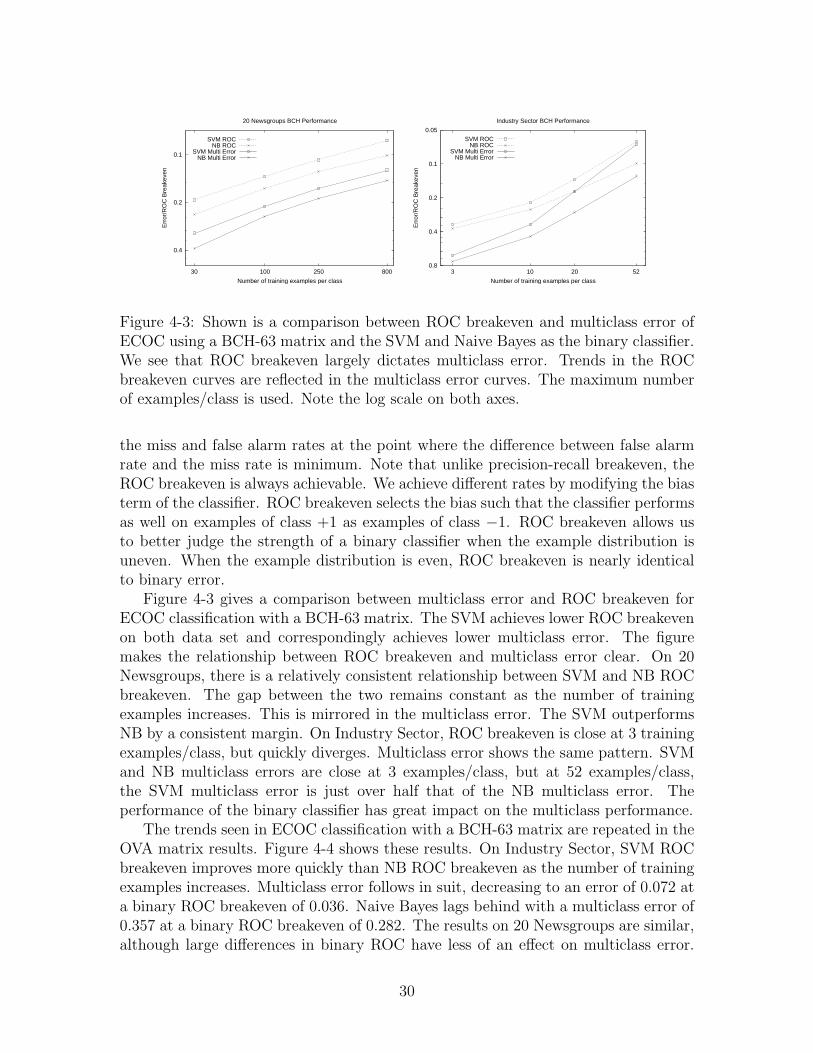
Figure 4-3 gives a comparison between multiclass error and ROC breakeven forECOC classification with a BCH-63 matrix. The SVM achieves lower ROC breakevenon both data set and correspondingly achieves lower multiclass error. The figuremakes the relationship between ROC breakeven and multiclass error clear. On 20Newsgroups, there is a relatively consistent relationship between SVM and NB ROCbreakeven. The gap between the two remains constant as the number of trainingexamples increases. This is mirrored in the multiclass error. The SVM outperformsNB by a consistent margin. On Industry Sector, ROC breakeven is close at 3 trainingexamples/class, but quickly diverges. Multiclass error shows the same pattern. SVMand NB multiclass errors are close at 3 examples/class, but at 52 examples/class,the SVM multiclass error is just over half that of the NB multiclass error. Theperformance of the binary classifier has great impact on the multiclass performance.

The trends seen in ECOC classification with a BCH-63 matrix are repeated in theOVA matrix results. Figure 4-4 shows these results. On Industry Sector, SVM ROCbreakeven improves more quickly than NB ROC breakeven as the number of trainingexamples increases. Multiclass error follows in suit, decreasing to an error of 0.072 ata binary ROC breakeven of 0.036. Naive Bayes lags behind with a multiclass error of0.357 at a binary ROC breakeven of 0.282. The results on 20 Newsgroups are similar,although large differences in binary ROC have less of an effect on multiclass error.

30

0.05

0.1

0.2

0.4

80025010030

Err

or/R

OC

Bre

akev

en

Number of training examples per class

20 Newsgroups One-vs-all Performance

SVM ROCNB ROC

SVM Multi ErrorNB Multi Error

0.04

0.08

0.16

0.32

0.64

3 10 20 52

Err

or/R

OC

Bre

akev

en

Number of training examples per class

Industry Sector One-vs-all Performance

SVM ROCNB ROC

SVM Multi ErrorNB Multi Error

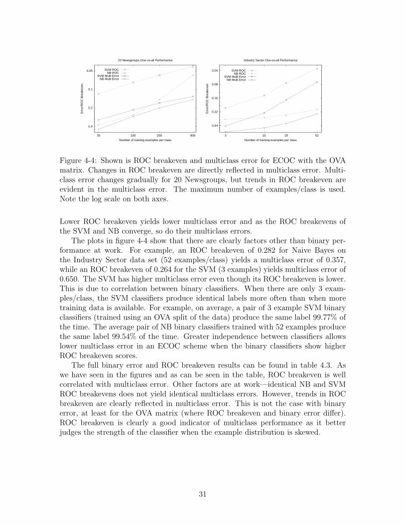
Figure 4-4: Shown is ROC breakeven and multiclass error for ECOC with the OVAmatrix. Changes in ROC breakeven are directly reflected in multiclass error. Multi-class error changes gradually for 20 Newsgroups, but trends in ROC breakeven areevident in the multiclass error. The maximum number of examples/class is used.Note the log scale on both axes.

Lower ROC breakeven yields lower multiclass error and as the ROC breakevens ofthe SVM and NB converge, so do their multiclass errors.

The plots in figure 4-4 show that there are clearly factors other than binary per-formance at work. For example, an ROC breakeven of 0.282 for Naive Bayes onthe Industry Sector data set (52 examples/class) yields a multiclass error of 0.357,while an ROC breakeven of 0.264 for the SVM (3 examples) yields multiclass error of0.650. The SVM has higher multiclass error even though its ROC breakeven is lower.This is due to correlation between binary classifiers. When there are only 3 exam-ples/class, the SVM classifiers produce identical labels more often than when moretraining data is available. For example, on average, a pair of 3 example SVM binaryclassifiers (trained using an OVA split of the data) produce the same label 99.77% ofthe time. The average pair of NB binary classifiers trained with 52 examples producethe same label 99.54% of the time. Greater independence between classifiers allowslower multiclass error in an ECOC scheme when the binary classifiers show higherROC breakeven scores.

The full binary error and ROC breakeven results can be found in table 4.3. Aswe have seen in the figures and as can be seen in the table, ROC breakeven is wellcorrelated with multiclass error. Other factors are at work—identical NB and SVMROC breakevens does not yield identical multiclass errors. However, trends in ROCbreakeven are clearly reflected in multiclass error. This is not the case with binaryerror, at least for the OVA matrix (where ROC breakeven and binary error differ).ROC breakeven is clearly a good indicator of multiclass performance as it betterjudges the strength of the classifier when the example distribution is skewed.

31

20 Newsgroups 800 250 100 30SVM NB SVM NB SVM NB SVM NB

OVA/Error 0.015 0.039 0.021 0.027 0.03 0.042 0.044 0.049OVA/ROC 0.043 0.059 0.059 0.146 0.078 0.262 0.118 0.375BCH/Error 0.079 0.101 0.105 0.121 0.135 0.151 0.194 0.224BCH/ROC 0.081 0.101 0.108 0.127 0.138 0.163 0.193 0.237

Industry Sector 52 20 10 3SVM NB SVM NB SVM NB SVM NB

OVA/Error 0.003 0.008 0.005 0.009 0.007 0.009 0.009 0.010OVA/ROC 0.036 0.282 0.075 0.378 0.141 0.428 0.264 0.473BCH/Error 0.062 0.100 0.137 0.176 0.218 0.253 0.347 0.376BCH/ROC 0.063 0.099 0.137 0.175 0.219 0.253 0.348 0.378

Table 4.3: Shown are binary errors and ROC breakeven points for the binary classifierstrained according to the matrix columns. Results for the Dense matrix are omittedsince they are nearly identical to the BCH results. Table entries are averaged over allmatrix columns and 10 train/test splits. Error is a poor judge of classifier strengthfor the OVA matrix. Error increases with more examples on 20 Newsgroups. Notethat error and ROC breakeven numbers are very similar for the BCH matrix.

20 Newsgroups Hinge LinearOVA/SVM 0.131 0.131OVA/NB 0.146 0.146BCH 63/SVM 0.125 0.126BCH 63/NB 0.145 0.144

Industry Sector Hinge LinearOVA/SVM 0.072 0.072OVA/NB 0.357 0.357BCH 63/SVM 0.067 0.067BCH 63/NB 0.128 0.127

Table 4.4: Shown are multiclass errors on two data sets and a variety of ECOCclassifiers. Errors are nearly identical between the hinge and linear loss functions.Although ECOC provides opportunity for non-linear decision rules through the lossfunction, the use of a non-linear loss function provides no practical benefit.

32

4.4.3 Non-linear loss does not affect ECOC performance

Another factor which can greatly impact ECOC multiclass error is the loss function.We use the hinge function for our experiments, g(z) = (1−z)+, which exhibits a non-linearity at z = 1. Using this loss function allows ECOC to express functions thatlinear classifiers, such as Naive Bayes and the linear SVM, cannot express. However,the fact that ECOC is non-linear does not provide empirical benefit, at least in ourexperiments. Table 4.4 shows results of experiments that we ran to compare thehinge loss function to a trivial linear loss function, g(z) = −z. We find practically nodifference in multiclass error compared to using the hinge loss function. The resultswe show use the maximum number of training examples (up to 52/class for IndustrySector and 800/class for 20 Newsgroups), but results are similar when fewer trainingexamples are used. The confidence information contributed by the loss function isimportant for text classification, but non-linearity provides no practical benefit. Thelinear loss function yields a completely linear system (since both our NB and SVMclassifiers are linear). This contributes evidence that text classification with bag-of-words representation is a linear problem.

33

Chapter 5

Feature Selection

Feature selection is an essential part of text classification. Document collections have10,000 to 100,000 or more unique words. Many words are not useful for classification.Restricting the set of words that are used for classification makes classification moreefficient and can improve generalization error. We describe how the application of In-formation Gain to feature selection for multiclass text classification is fundamentallyflawed and compare it to a statistics-based algorithm which exhibits similar difficul-ties. A text feature selection algorithm should select features that are likely to bedrawn from a distribution which is distant from a class-neutral distribution. Neitherof the two algorithms do this. We describe a framework for feature selection thatencapsulates this notion and exposes the free parameters which are inherent in textfeature selection. Our framework provides a basis for new feature selection algorithmsand clarifies the intent and design of such algorithms.

5.1 Information Gain

Information gain (IG) is a commonly used score for selecting words for text clas-sification [Joachims, 1997; McCallum and Nigam, 1998; Yang and Pedersen, 1997;Mitchell, 1997]. It is derived from information theoretic notions. For each word,IG measures the entropy difference between the unconditioned class variable and theclass variable conditioned on the presence or absence of the word,

IG = H(C)−H(C|Wk) =∑c∈C

∑wk∈{0,1}

p(c, wk) logp(c|wk)p(c)

. (5.1)

This score is equivalent to the mutual information between the class and word vari-ables, IG = I(C;Wk). Hence, this score is sometimes called mutual information. Theprobabilities correspond to individual word occurrences. wk = 1 corresponds to theoccurrence of word wk. wk = 0 corresponds to the occurrence of some other word.We treat every token in the data as a binomial event and estimate the probabilities inequation 5.1 via maximum likelihood. Let f ck be the number of occurrences of word

34

wk in class c (fk =∑

c fck). Let N c =

∑k f

ck (N =

∑cN

c). Then

IG =∑c∈C

f ck/N logf ck/fkN c/N

+ (N c − f ck)/N log(N c − f ck)/(N − fk)

N c/N. (5.2)

For feature selection, IG is computed for every word and words with larger scores areretained.

5.2 Hypothesis Testing

A desirable property of a feature is for its distribution to be highly dependent on theclass. Words that occur independent of the class give no information for classifica-tion. A natural approach to developing a metric for filtering features is to determinewhether each word has a class-independent distribution and to eliminate the word ifit has such a distribution. In statistics, the problem of determining whether data isgenerated from a particular distribution is known as hypothesis testing. One proposesa model and parameters and ranks data according to its likelihood.

For text feature selection, we call this feature selection score HT. We consider asingle word, wk, and treat its fk appearances in the training data as fk draws from amultinomial where each event is a class label. Our hypothesized parameters are p ={N c/N}. These parameters correspond to word occurrence being irrelevant of class,i.e. θ1

k = · · · = θmk in the multinomial model. Our test statistic, which determines theordering of data, is the difference in log-likelihoods between a maximum likelihoodestimate, p = {f ck/fk}, and the hypothesized parameters,

HT (p, p) = 2[l(p)− l(p)] = 2∑c

f ck logf ck/fkN c/N

. (5.3)

HT > 0 always and larger HT values correspond to data that is less likely to havebeen generated by the proposed model. We keep words with large HT values anddiscard words with small HT values. Note that this score is similar to the IG score.

5.3 The Generalization Advantage of Significance

Level

It is common for feature selection to be performed in terms of the number of features.For example, when using the IG score, one does not usually select an IG cutoff andeliminate all words with IG score less than that. Rather, one ranks words by their IGscore and retains the top N scoring words. However, the number of words that shouldbe retained for a particular application varies by data set. For example, McCallumand Nigam found that the best multinomial classification accuracy for the 20 News-groups data set was achieved using the entire vocabulary (62,000+ words) [1998]. Incontrast, they found that the best multinomial performance on the “interest” cate-

35

gory of the Reuters data set was achieved using about 50 words. An advantage ofthe HT score is that the number of words to be selected can be specified in terms ofa significance level. Let HTcut be the chosen cutoff HT score. The significance levelcorresponding to HTcut is

SL = Pr{HT (p, p) ≥ HTcut| p is a sample estimate of p}. (5.4)

p is fixed; p is variable. SL = 0.10 selects words with empirical distributions that oc-cur in only 10% of draws from the hypothesis distribution; selected words are atypicalof the class-neutral distribution. This is more intuitive than simply selecting an HTor IG cutoff and may allow generalization across different data sets and conditions.Using significance level to choose a number of words for feature selection gives aneasy-to-interpret understanding of what words are retained.

5.4 The Undesirable Properties of IG and HT

The application of IG and HT to text classification ignores critical aspects of text.Most words occur sparsely and only provide information when they occur. IG expectsa word to provide information when it does not occur. Both IG and HT have atendency to give higher scores to words that occur more often. For example, ifp = {1/2, 1/2}, p = {2/5, 3/5} and fk = 10000, HT ≈ 201.3. More than 99.9% ofdraws from p have a HT score less than 201.3. However, words which are devoid ofclass information have such empirical distributions. They are given a high score byIG and HT because they provide a significant reduction in entropy and there is littlechance that they could have been drawn from the hypothesis distribution. The factthat the true distribution is probably very close to the hypothesized distribution isignored by IG and HT. A word that occurs just a few times (e.g. fk = 7) can neverhave a high IG or HT score because its non-occurrences provide little information andsince the most extreme empirical distribution is a relatively common draw from thehypothesis distribution. For example, the chance of observing p = {1, 0} or p = {0, 1}from 7 draws of a multinomial with parameters p = {1/2, 1/2} is 2/27 ≈ 0.0156.

The appearance of a single word can sometimes be used to predict the class (e.g.“Garciaparra” in a “baseball” document). However, a non-appearance is rarely in-formative (e.g. “Garciaparra” won’t appear in all “baseball” documents). A textfeature selection algorithm should retain words whose appearance is probably highlypredictive of the class. In this sense, we want words that are discriminative.

5.5 Simple Discriminative Feature Selection

A simple score for selecting discriminative features is

S = argmaxc p(c|wk), (5.5)

36

p = {1/2,1/2}

p = {1,0}

εp = {2/3,1/3}

p = {8/9,1/9}

p = {5/6,1/6}

Figure 5-1: Our new feature selection framework views text feature selection as aproblem of finding words (their empirical distribution represented by p) which areunlikely to have a true distribution, p, within ε of the class independent distribution,p. The dashed arrows point to distributions from which p could have been drawn.

where p(c|wk) is the probability of the class being c given the appearance of wordwk. This gives the largest score to words which only appear in a single class. If sucha word appears in a document, we know without a doubt what class that documentbelongs to. We cannot find p(c|wk), but we can make an estimate of it based on p.A MAP estimate with Dirichlet {αc = 2} prior gives us

S = argmaxcf ck + 1

fk +m. (5.6)

The setting of these hyper-parameters encode a preference for the uniform distribu-tion, but there is no reason to believe that other choices are not more appropriate.The choice of prior is important as it serves as a measure of confidence for the empir-ical distribution. If the prior is a Dirichlet that prefers the class-neutral distributionover all others, {αc = cN c/N}, the estimate of p for a word lies on the line connectingp and p. The prior dictates how close to p the estimate is for a given number of draws.

5.6 A New Feature Selection Framework

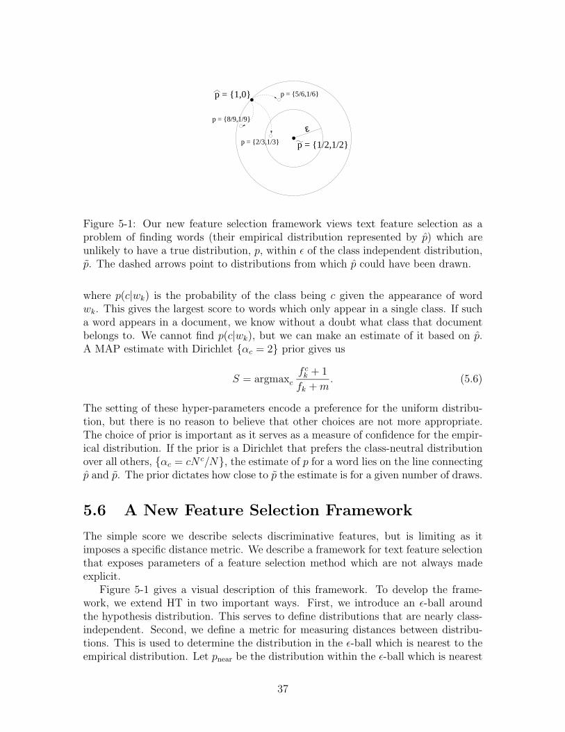
The simple score we describe selects discriminative features, but is limiting as itimposes a specific distance metric. We describe a framework for text feature selectionthat exposes parameters of a feature selection method which are not always madeexplicit.

Figure 5-1 gives a visual description of this framework. To develop the frame-work, we extend HT in two important ways. First, we introduce an ε-ball aroundthe hypothesis distribution. This serves to define distributions that are nearly class-independent. Second, we define a metric for measuring distances between distribu-tions. This is used to determine the distribution in the ε-ball which is nearest to theempirical distribution. Let pnear be the distribution within the ε-ball which is nearest

37

to p. HT judges the possibility of p being drawn from p. In the new framework,we evaluate the probability of p being drawn from pnear. We select words that arelikely to have distributions outside of the ε-ball—distributions which are far fromthe class-independent distribution. So, the new feature selection framework has asparameters

• ε, to define a set of distributions close to p,

• a metric, d(p, q), to determine pnear, and

• a significance level, SL, for comparing empirical and true distributions.

As before, we use a hypothesis test score to define significance level,

NHT (p, pnear) = 2[l(p)− l(pnear)]. (5.7)

Given a cutoff choice for NHT, the significance level is defined as

SL = Pr{NHT (p, pnear) > NHTcut| p is a sample estimate of pnear}. (5.8)

A word (p) is selected iff NHT (p, pnear) > NHTcut where NHTcut is defined by thechosen significance level and pnear is the distribution in the ε-ball that is closest to p(defined by d(p, pnear)). Since words with empirical distributions near p are discarded,a smaller cutoff and larger significance level can be used. Thus, NHT will includemore discriminative words than IG or HT for the same number of selected features.

This new framework exposes the fundamental parameters variables in a text fea-ture selection scheme where only word appearances are used. ε compensates for thefact that words are not truly drawn from a multinomial by eliminating words thatare close to the class-neutral distribution. SL allows the user to select the amount ofevidence required to show that a word is not drawn from a class-neutral distribution.d(p, q) defines the closeness of two distributions and specifies (along with ε) to whichdistribution empirical distributions should be compared. This new framework selectswords that are likely to be drawn from a discriminative distribution. Unlike HT andIG, it accounts for the fact that text is not a multinomial and empirical distributionsthat are close to the class-neutral distribution are unlikely to be informative withrespect to the class variable.

38

Chapter 6

Conclusion

The focus of this thesis has been the application of Naive Bayes to multiclass text clas-sification and has resulted in several new insights. Our parameter estimate analysisshows that Naive Bayes performs poorly when one class has relatively few examples.We also empirically showed that ECOC performance is mainly a result of binaryperformance. When the binary classifiers in ECOC have sufficient examples, ECOCperforms much better than regular Naive Bayes. Furthermore, we showed that acommonly-used text feature selection algorithm is not good for multiclass text clas-sification because it judges words by their non-appearances and has a bias to wordsthat appear often. We proposed to select features by whether or not their distributionis discriminative and gave a framework which exposes the free parameters in such ascheme.

In terms of future work, the choice of the prior can greatly affect classification,especially for words with few observations, but its choice is not well understood. Bet-ter selection of the prior may lead to improved classification performance. Moreover,we along with others have observed that linear classifiers perform as well or betterthan non-linear classifiers on text classification with a bag-of-words representation.Determining whether this is generally true and understanding why this is the case isimportant. In our ECOC experiments, the performance of a particular matrix var-ied by data set and the amount of training data. Additional gains may be possibleby developing algorithms to successively tune the columns of the ECOC matrix tothe specific problem. We also envision to be able to use unlabeled data with EM tocounter the limiting effect of classes with only a few labeled examples.

39

Appendix A

Data Sets

For our experiments, we use two different commonly used data sets [McCallum andNigam, 1998; Slonim and Tishby, 1999; Berger, 1999; Ghani, 2000].We use McCal-lum’s rainbow to pre-process the documents [1996].

20 Newsgroups is a data set collected and originally used for text classificationby Lang [1995b] [Lang, 1995a]. It contains 19,974 non-empty documents evenly dis-tributed across 20 categories, each representing a newsgroup. We remove all headers,UU-encoded blocks and words which occur only once in the data. The vocabularysize is 62061. We randomly select 80% of documents per class for training and theremaining 20% for testing. This is the same pre-processing and splitting as McCallumand Nigam used in their 20 Newsgroups experiments [McCallum and Nigam, 1998].

The Industry Sector data is a collection of corporate web pages organized intocategories based on what a company produces or does [Nigam, 2000]. There are 9619non-empty documents and 105 categories. We remove headers, prune stoplist wordsand words that occur only once. We include HTML for our experiments. However,we find that regular Naive Bayes and ECOC with OVA and Naive Bayes do betterwhen HTML is first removed. The difference does not change our conclusions, butis of note. Our vocabulary size is 55197. We randomly select 50% of documents perclass for training and the remaining 50% for testing. We create subsets of the trainingset to observe the effects of varying amounts of training data. This is similar to thepre-processing and splitting as Ghani used in his Industry Sector experiments [Ghani,2000]. The only difference is that Ghani excluded HTML in his pre-processing.

Text classification experiments often include a feature selection step which mayimprove classification. McCallum and Nigam performed feature selection experimentson a modified version of the Industry Sector data set and the 20 Newsgroups dataset; in neither case did feature selection significantly improve classification [1998].In our own experiments, we found information gain feature selection to not improveclassification. We use the full vocabulary for all of our experiments.

40

Bibliography

[Allwein et al., 2000] Erin L. Allwein, Robert E. Schapire, and Yoram Singer. Re-ducing multiclass to binary: A unifying approach for margin classifiers. Journal ofMachine Learning Research, 1:113–141, 2000.

[Berger, 1999] Adam Berger. Error-correcting output coding for text classification. InProceedings of IJCAI-99 Workshop on Machine Learning for Information Filtering,Stockholm, Sweeden, 1999.

[Chakrabarti et al., 1997] Soumen Chakrabarti, Byron Dom, Rakesh Agrawal, andPrabhakar Raghavan. Using taxonomy, discriminants and signatures for navigatingin text databases. In Proceedings of the 23rd VLDB Conference, 1997.

[Cover and Thomas, 1991] Thomas Cover and Joy Thomas. Elements of InformationTheory. John Wiley & Sons, Inc., 1991.

[Dietterich and Bakiri, 1991] Tom G. Dietterich and Ghulum Bakiri. Error-correctingoutput codes: A general method for improving multiclass inductive learning pro-grams. In Proceedings of the Ninth National Conference on Artificial Intelligence,pages 572–577, Anaheim, CA, 1991. AAAI Press.

[Domingos and Pazzani, 1996] Pedro Domingos and Michael Pazzani. Beyond inde-pendence: conditions for the optimality of the simple bayesian classifier. In Pro-ceedings of the Thirteenth International Conference on Machine Learning (ICML),1996.

[Dumais et al., 1998] Susand Dumais, John Platt, David Heckerman, and MehranSahami. Inductive learning algorithms and reepresentations for text classification.In Seventh International Conference on Information and Knowledge Management,1998.

[Ferguson, 1973] T. S. Ferguson. A bayesian analysis of some nonparametric prob-lems. Annals of Statistics, pages 209–230, 1973.

[Freund and Schapire, 1996] Yoav Freund and Robert E. Schapire. Experiments witha new boosting algorithm. In Proceedings of the Thirteenth International Confer-ence on Machine Learning, 1996.

41

[Freund and Schapire, 1999] Yoav Freund and Robert E. Schapire. A short introduc-tion to boosting. Journal of Japanese Society for Artificial Intelligence, 14(5):771–780, 1999.

[Frietag and McCallum, 1999] Dayne Frietag and Andrew McCallum. Informationextraction with hmms and shrinkage. In Proceedings of the AAAI’99 Workshop onMachine Learning for Information Extraction, 1999.

[Ghani, 2000] Rayid Ghani. Using error-correcting codes for text classification. InProceedings of the Seventeenth International Conference on Machine Learning,2000.

[Guruswami and Sahal, 1999] Venkatesan Guruswami and Amit Sahal. Multiclasslearning, boosting and error-correcting codes. In Proceedings of the Twelfth AnnualConference on Computational Learning Theory, 1999.

[Joachims, 1997] Thorsten Joachims. Text categorization with support vector ma-chines: Learning with many relevant features. Technical report, University ofDortmund, Computer Science Department, 1997.

[Lang, 1995a] Ken Lang. 20 newsgroups. http://www.ai.mit.edu/people/jrennie/20Newsgroups,1995.

[Lang, 1995b] Ken Lang. Newsweeder: Learning to filter netnews. In Proceedings ofthe Twelfth International Conference on Machine Learning, pages 331–339, 1995.

[Lewis, 1998] David D. Lewis. Naive (bayes) at forty: the independence assumption ininformation retrieval. In Proceedings of the Tenth European Conference on MachineLearning, 1998.

[McCallum and Nigam, 1998] Andrew McCallum and Kamal Nigam. A comparisonof event models for naive bayes text classification. In Proceedings of the AAAI-98workshop on Learning for Text Categorization, 1998.

[McCallum, 1996] Andrew Kachites McCallum. Bow: A toolkit for sta-tistical language modeling, text retrieval, classification and clustering.http://www.cs.cmu.edu/∼mccallum/bow, 1996.

[Mitchell, 1997] Tom Mitchell. Machine Learning. McGraw-Hill Companies, Inc.,1997.

[Nigam, 2000] Kamal Nigam. Industry sector data. http://www.cs.cmu.edu/∼TextLearning/datasets.html, 2000.

[Rifkin, 2000] Ryan Rifkin. Svmfu. http://five-percent-nation.mit.edu/SvmFu/,2000.

[Ristad, 1995] Eric Svwn Ristad. A natural law of succession. Technical ReportCS-TR-495-95, Princeton University, 1995.

42

[Slonim and Tishby, 1999] Noam Slonim and Naftali Tishby. Agglomerative informa-tion bottleneck. In Neural Information Processing Systems 12 (NIPS-99), 1999.

[Vapnik, 1995] Vladimir Vapnik. The Nature of Statistical Learning Theory. Springer-Verlag, 1995.

[Yang and Pedersen, 1997] Yiming Yang and J. O. Pedersen. A comparitive studyon feature selection in text categorization. In Proceedings of the Fourteenth Inter-national Conference on Machine Learning, 1997.

43