jason modisette, energy solutions jerry modisette, consultant … · 2017-06-25 · jerry...

Energy Solutions International - Energy Solutions, Delivered

Physics of Pipeline Flow Jason Modisette, Energy Solutions Jerry Modisette, Consultant for Energy Solutions 2003 This paper is copyrighted to the Pipeline Simulation Interest Group and has been re-printed with the permission of PSIG.

Energy Solutions International All Rights Reserved www.energy-solutions.comEnergy Solutions International All Rights Reserved www.energy-solutions.com

World leaders in pipeline management.

ABSTRACT

This paper discusses the current understanding of aspects of the physics of fluid flow in pipelines relevant to pipeline flow simulations. Topics include fluid properties, the laminar/turbulent transition, friction (including methods of drag reduction), energy flow and dissipation, and the effect of more than one phase in the pipeline. Practical issues are described in terms of fundamental physics, as contrasted with an empirical approach.

INTRODUCTION

Flow through tubes was the subject of some of the earliest attempts to understand the physics of fluid flow. Reynolds’ original experiments on turbulence were done with ink streams in water flowing in tubes. Steady-state axial laminar flow in a cylinder is one of the few fluid flow problems for which an exact solution of the fundamental flow equations can be found. Flow in pipelines is usually analyzed by numerical simulations based on a special case of the Navier-Stokes equations for fluid flow, in which the viscous stresses are consolidated into a friction force term based partly on physics and partly on empirical results. The Navier-Stokes equations are essentially expressions of the conservation of mass and momentum. Only in recent years has the flow and dissipation of energy been added to such simulations. There remain substantial shortcomings in the understanding of the laminar-turbulent transition and in the definition and effect of varying fluid properties. The understanding of pipeline hydraulic operations involves forces, motion, and energy transformations, which are the elements of what we call the physics of pipeline flow. Our objective in this paper is to present a review of the current state of this understanding, including some of its history, and calling attention to notable deficiencies.

WHO CARES ABOUT THE PHYSICS?

It is possible to design, build, and operate a pipeline using rules of thumb and practical experience, with no reference to the underlying fundamentals. We believe this approach is fraught with hazard, because pipelines and their modes of operation vary a great deal. The physics do not vary, although there are some things not well understood. Knowing what isn’t understood is also useful. So, pipeliners should care about the physics.

FLUID PROPERTIES – LIQUIDS VS. GASES

An unfortunate, in our opinion, development in the practice of pipeline simulation has been a tendency to treat gas and liquid pipelines separately, even though the flow equations and the numerical methods are the same. With an appropriate equation of state and minor adjustments in time and distance steps, a good simulator can be used for either gases or liquids. Devices, on the other hand, especially pumps, compressors, and throttling valves, behave differently for liquids and gases.

Energy Solutions International Whitepaper

2



Liquids and gases have different macroscopic properties arising from the fundamental differences in the two types of fluid. It is a strength of the pipe flow equations, which are essentially expressions of the conservation of the fundamental quantities, mass, momentum, and energy, that the same equations and methods work for both. On a molecular level, the major difference between liquids and gases is that liquid molecules are always in contact with their nearest neighbors, while gas molecules are separated except during collisions. This difference produces large differences in three macroscopic properties: density, compressibility and viscosity. At atmospheric conditions, liquids are typically three orders of magnitude denser than gases. At most pipeline pressures, the difference is less, but still large. At very high pipeline pressures, the density of a typical hydrocarbon gas approaches the density of the liquid form of the hydrocarbon, and the distinction between gas and liquid disappears. Gases are more compressible than liquids for the simple reason that compressing a gas reduces the space between the molecules, while compressing a liquid involves squeezing the molecules themselves. Since liquid molecules are in contact with their nearest neighbors, when a liquid is compressed the individual molecules are deformed so as to jostle them into more compact structures. When a gas is compressed, reducing their space between the molecules does not require that they be deformed. A liquid resists compression more than a gas because the collective force required to deform a liquid’s molecules is greater than the increased collision rate with the container wall that produces increased pressure in a gas. The relationship between the pressure, temperature, and density of a fluid is called the Equation of State. Equations of state for pipeline fluids are discussed in detail in Reference 1. Both liquids and gases resist shear flow; this resistance is the phenomenon we call viscosity. Shear flow refers to parallel flow in which the flow speed varies across the flow, as illustrated below:

For liquids, the resistance to shear flow is caused by the molecules rubbing against one another. For gases, migration of fast molecules into the slower stream (and vice versa) due to random molecular motion causes this resistance as the migrating molecules come to equilibrium with their new environment. In both cases, the viscosity is caused by a transfer of momentum-along-the-stream across the stream; this illustrates a principle that we see repeatedly in pipeline physics: that momentum can be transferred either by one part of the system


3



exerting a force on another part (as in the case of liquid viscosity) or by momentum-carrying bodies moving from one part of the system to another (as in the case of gas viscosity). There are several practical results of these differences, from a pipeline point of view: • The higher density of liquids makes the effect of elevation changes greater than for gases, since the

change in hydrostatic head due to an elevation change is proportional to the density of the fluid. • The higher resistance of liquids to compression makes changes propagate faster, and makes inertial

phenomena, such as water hammer, larger. • The compressibility of gases makes heating or cooling due compression/expansion work a significant

factor in the energy balance of gases. • The higher viscosity of liquids makes the laminar/turbulent transition more important (and a source of more

difficulty) for liquids. • The different behaviors of the viscosity make temperature effects qualitatively different. For example, for a

constant mass flow, the frictional resistance to gas flow goes up as the temperature rises, while the frictional resistance to liquid flow goes down.

These important practical differences will be discussed in more detail as we get into describing the related phenomena.

KINEMATICS

THE FLUID ELEMENT Analysis of what exactly is going on in a pipeline must begin with the choice of which part of the system to examine. The pipeline as a whole includes not only the transported fluid but also pipe walls, the surrounding soil, compressors or pumps, and other equipment. We will examine only the fluid itself at this point; however, we still must choose which part of the fluid to look at. The easiest system to analyze is a thin slice of fluid taken across a vertical cross-section of the pipe, which will be called the fluid element (Figure 1). This slice is chosen to have an infinitesimal length dx so that all properties of the fluid can change only linearly from the upstream side of the slice to the downstream side. However, in the figure it is drawn with finite width for clarity. The total of all gas or liquid in a pipeline is just a series of these slices stacked like a roll of coins. The interesting properties of the fluid are the pressure, temperature, and flow velocity. The fluid density and viscosity can be computed from the pressure and temperature by look-up tables or empirical equations based on experiment. The fluid element at distance x from the start of the pipe is chosen so as to have pressure

, velocity , and so on at its center. (See Appendix I for variable definitions). This element also

has a local pressure gradient (rate of change of pressure with distance

)(xP )(xv

x ) of dxdP , a local velocity gradient

of dxdv , etc. Since each fluid element has deliberately been defined to be very short, the pressure at the

downstream side of the fluid element at x is dxxdPdxxP )(2/1)( + , and higher order terms such as

22

dxPd can be ignored. This is a nice property of infinitesimal distances like the thickness of the fluid


4



element dx. Similarly, the pressure at the upstream side of the element is dxxdPdxxP )(2/1)( − , and

the average pressure across the element is . )(xP COORDINATE SYSTEMS This article will mostly treat the fluid flow in the pipe as one-dimensional, meaning that for a given x the fluid properties and values of the dynamic variables are the same at any radial distance from the center of the pipe. While this isn't true, the effects caused by radial variations can be included entirely inside the friction factor (for single-phase flow, which is the only sort considered here). Pipes often run up and down hills, the elevation at

x will be called and therefore the local slope will be )(xz dxdz .

FORCES AND MOTION

The small volume of fluid shown in Figure 1 must conserve mass, momentum, and energy. This means that the net flow of each of these quantities into the fluid element (net flow meaning the total flow in minus the total flow out) must equal the rate of buildup of that quantity inside the element. The justification for this is the most straightforward for conservation of mass: all mass in this system exists in the form of molecules of fluid, and molecules don't just appear or disappear: if a molecule flows into the fluid element, it must either still be there at a later time or it must have flowed out again. If the pipe diameter at x , the location of the fluid element, is the cross-sectional area is )(xD

4)()(

2xDxA π=

and the rate at which mass flows into the element is

)()()()( xvxAxxQ upupup ρ=

where the upstream density and velocity are

dxddxxxupρρρ

21)()( −=

dxdvdxxvxvup 2

1)()( −=

and the downstream quantities are

)()()()( xvxAxxQ dndndn ρ=

with downstream density and velocity defined

dxddxxxdnρρρ

21)()( +=

dxdvdxxvxvdn 2

1)()( +=

The total volume of the fluid element at x is dxxAxV )()( =

and the mass contained within it is just that volume multiplied by the average density )(xρ )()()( xdxxAxmass ρ=


5



The conservation law stated above for mass can be written in terms of these variables that over a time interval dt,

),(),(),(),( txdtQtxdtQtxmassdttxmass dnup −+=+

which, with a little algebra, dividing both sides by , leads to the differential form of the conservation

of mass,

dxdtxA )(

0)(=+

dxvd

dtd ρρ

This exact mathematical reasoning can be used to generate similar equations for conservation of momentum and energy. FORCES ON A FLUID ELEMENT Just as the net number of molecules (and therefore the mass) flowing into a fluid element over a time interval must equal the buildup of mass in that element over that interval, the net momentum carried into the interval must equal the buildup of momentum. However, as we saw earlier in the discussion of viscosity, momentum has one major difference from mass in this respect: momentum can enter and leave the fluid element not only by being carried in and out by molecules, but also by flowing in and out as forces. A force is equivalent to a flow of momentum. There are a number of important forces in a pipe. The first is the force of pressure: the molecules outside the fluid element in the upstream direction are bouncing around due to their thermal energy (and bouncing with a much higher velocity than the average forward velocity of the overall flow) and they are bouncing into the molecules in the fluid element, pushing them downstream. Similarly, the molecules outside the downstream boundary are bouncing off molecules inside the element, pushing the fluid inside the element upstream. The upstream force due to this bouncing is

( ) )()( xAxPxF upup =

where the pressure at the upstream side of the element is

⎟⎠⎞

⎜⎝⎛−=

dxdPdxxPxPup 2

1)()(

and the downstream force is

( ) )()( xAxPxF dndn =

where the downstream pressure is

⎟⎠⎞

⎜⎝⎛+=

dxdPdxxPxPdn 2

1)()(

so the net force from pressure is

dxdPxdxAxFxF dnup )()()( −=−

which is proportional to the pressure gradient at x .


6



Note that this source of momentum transfer is NOT the same as momentum being carried into our out of the fluid element by the molecules flowing through it; that term must be accounted for separately in the conservation of momentum. A second force on the fluid element is the force of friction with the pipe wall. If in reality all the fluid throughout the cross-section of the pipe flowed at the same velocity for a given value of )(xv x , then the one-

dimensional approximation could be kept here, but it doesn't. For laminar pipe flow, the velocity profile changes quadratically with radius between a maximum value at the center of the pipe and zero at the wall; in turbulent flow, there are complicated turbulent eddies but the average velocity is constant except for a laminar boundary layer near the wall, in which it rapidly drops to zero. Since the laminar flow problem can be solved exactly, the friction force can be shown to be

)()()()()()( xDxvxvxxdxfxFfric πρ−=

where is the average fluid velocity (averaged over the cross-section of the pipe). This average is

the same as the one-dimensional defined earlier, so this foray into multiple dimensions can now be

terminated.

)(xv )(xv)(xv

The laminar friction factor (also obtained from the exact solution) is:

)Re(64)( xxf =

where Re is the Reynolds number for the flow,

)()()()()Re(

xxDxvxx

µρ

=

For turbulent flow, the same form of the friction force function may be used, but the friction factor is different. It is much larger, and the Reynolds number dependence is different. Pipe wall roughness also has an effect. No exact solution for the turbulent friction factor has been found. A widely used correlation partly based on the physics is the Colebrook-White friction factor. Sometimes adjustments in the friction factor are required to make the resulting pressure drop/flow correlation correspond to data. In real-time simulations common practice is to make adjustments automatically using a feedback algorithm, which also takes into account possible measurement errors. This process is usually referred to as tuning. The final external source of momentum (force) is that due to gravity. Unlike the pressure gradient force and the frictional force, which were “pushing” on the borders of the fluid element, the force of gravity always pushes the entire contents of the fluid element straight down. This downwards force can be broken up into a component parallel to the pipe and a component perpendicular to the pipe. The pipe wall pushes back against the perpendicular component, which cancels it out. The parallel component, however, does exert a net force on the fluid,

dxdzgxmassxFgrav )()( −=

or, writing out the earlier definition for the mass contained in the fluid element,


7



dxdzdxxgAxxFgrav )()()( ρ=

Therefore the net force on the fluid element, including both friction and gravity, is

⎢⎣⎡−=

dzdzxgAxdxxFnet )()()( ρ ⎥⎦

⎤−−dxdPxAxDxvxvxxf )()()()()()( πρ

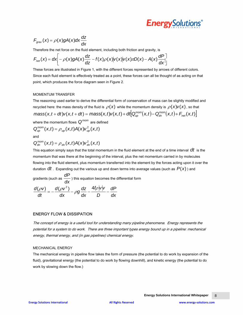
These forces are illustrated in Figure 1, with the different forces represented by arrows of different colors. Since each fluid element is effectively treated as a point, these forces can all be thought of as acting on that point, which produces the force diagram seen in Figure 2. MOMENTUM TRANSFER The reasoning used earlier to derive the differential form of conservation of mass can be slightly modified and recycled here: the mass density of the fluid is )(xρ while the momentum density is )()( xvxρ , so that

=++ ),(),( dttxvdttxmass ( ) ( )[ ]),(,,),(),( txFtxQtxQdttxvtxmass netmomdn

momup +−+

where the momentum flows are defined momQ),()(),(),( 2 txvxAtxtxQ upup

momup ρ=

and

),()(),(),( 2 txvxAtxtxQ dndnmomdn ρ=

This equation simply says that the total momentum in the fluid element at the end of a time interval is the momentum that was there at the beginning of the interval, plus the net momentum carried in by molecules flowing into the fluid element, plus momentum transferred into the element by the forces acting upon it over the duration . Expanding out the various up and down terms into average values (such as ) and

gradients (such as

dt

dt )(xP

dxdP

) this equation becomes the differential form

dxdP

Dvvf

dxdzg

dxvd

dtvd

−−−−=ρ

ρρρ 4)()( 2

ENERGY FLOW & DISSIPATION

The concept of energy is a useful tool for understanding many pipeline phenomena. Energy represents the potential for a system to do work. There are three important types energy bound up in a pipeline: mechanical energy, thermal energy, and (in gas pipelines) chemical energy. MECHANICAL ENERGY The mechanical energy in pipeline flow takes the form of pressure (the potential to do work by expansion of the fluid), gravitational energy (the potential to do work by flowing downhill), and kinetic energy (the potential to do work by slowing down the flow.)


8



Since expansion of a liquid is small, the pressure energy contained in the liquid might at first also seem to be unimportant. However, a small change in volume in a liquid is associated with a large change in pressure. This means that a small degree of compression of a liquid can put the same amount of mechanical energy into it as much greater compression of a gas. In both gas and liquid pipelines pressure is the means for transmitting the energy from the compressor or pump down the pipeline. The gravitational energy depends on the fluid density and the elevation. For liquid pipelines with large elevation changes, managing the gravitational energy can be a major activity, while for a gas pipeline with small elevation changes gravitational energy may be insignificant. The kinetic energy of fluid motion is insignificant in the normal operation of a pipeline. However, in the case of a leak, the kinetic energy of fluid motion in the hole usually determines the leak rate, directly in the case of a liquid, and indirectly in the case of a gas. THERMAL ENERGY Thermal energy is the energy of motion of the molecules, including translation, vibration, and rotation. Liquid molecules have little translational or rotational energy. Vibration, including the collective vibrations of neighboring molecules, is the principal molecular motion in a liquid. In a gas the molecules are moving at a high speed and, depending on the structure of the molecule, the gas molecules may be rotating and vibrating. Thermal energy is important because mechanical energy is converted into thermal energy through compression and friction, and thermal energy is converted into mechanical energy through expansion. The treatment of thermal energy in pipeline simulations is discussed in detail in reference 2. THERMODYNAMICS Thermodynamics is the field of physics concerned with the conversions between thermal and mechanical energy, and with the limitations on these conversions due to the fundamental nature of entropy, which is described below. Many thermodynamic quantities have been defined which have associated laws. Two such quantities are of concern to us: entropy and enthalpy. The change in the entropy of a system is usually of more importance than the absolute value. The change in entropy is the heat added or lost divided by the absolute temperature of the system. The second law of thermodynamics says that the total change in entropy in a system during any process cannot be negative. In a pipeline, mechanical energy is converted into heat by work against friction. This heat is added to the fluid, so that the entropy change is positive. The second law of thermodynamics says that this process never reverses itself, with the frictional heat doing work to move the fluid against the pressure gradient. This conforms to our observations. Enthalpy is the thermal energy plus the pressure energy. Enthalpy is a useful concept because a compressible fluid exchanges mechanical energy with its environment when it expands or is compressed. It may also exchange thermal energy. Thinking in terms of the enthalpy lets one implicitly take the environmental interactions into account in an energy balance.


9



A completely insulated pipeline flows at constant enthalpy. The work against friction comes from the thermal and pressure energy of the fluid. This energy goes into the fluid as heat, so that the enthalpy gained in the form of thermal energy equals the thermal and pressure energy lost. For an ideal gas, flow at constant enthalpy is at constant temperature. For a liquid, the temperature increases. For real gases, the temperature decreases. These differences are because of the differences in the forces between the molecules, which are part of the chemical energy. CHEMICAL ENERGY Energy flow in liquid pipelines can be described without recourse to chemical energy, but in gases that part of the system's energy bound up in long-range intermolecular interactions leads to the Joule-Thompson Effect, which is a significant contributing factor to fluid temperature during expansion or decompression. We will call the energy that represents potential of long-range intermolecular forces to do work during expansion of the fluid "chemical energy". The difference between chemical energy and pressure is that all the effects of pressure come from the fluid molecules whacking into each other, and would be unchanged if the molecules were tiny billiard balls (of the molecules’ mass) instead of molecules. Chemical energy is important because as a gas expands rapidly, the molecules must fight attractive forces between them, and use up some of the system's thermal energy in the process. This results in cooling of the gas as it expands. This effect is most dramatic during rapid expansion such as in a gas line rupture, during which the gas near the rupture can become so cold that it makes the pipe walls brittle. In some gases and some temperatures, the intermolecular forces can be repulsive rather than attractive, which leads to heating as the gas expands - this is never the case in natural gas pipelines, however. An ideal gas does not exhibit Joule-Thompson cooling because it IS assumed to be made of tiny billiard balls, and therefore there are no interactions between the particles other than billiard-ball-like collisions.

THERMODYNAMIC CYCLES

One way to look at the energy flow in a system is the thermodynamic cycle. A thermodynamic cycle is a graph of the relation between two thermodynamic quantities as the process goes around its cycle. Strictly speaking, a pipeline doesn’t go through a cycle. We will consider a pseudo cycle going from one station’s suction to the next station’s suction. The variables that produce the most illustrative cycle are pressure and volume. The work for any part of the cycle is the area under the PV curve for that part of the cycle. The net work done during the cycle is the area inside the cycle on the graph. In a pipeline work is done on the fluid by pumps or compressors, while the fluid does work against friction. Gravitational work may be by or on the fluid, depending on whether the pipe is going uphill or downhill.


10



Figure 3 shows an idealized thermodynamic cycle for a level gas pipeline. The cycle is idealized because the suction pressures, temperatures, and volumes are the same at two consecutive stations. The compression cycle is isentropic, which is a reasonably accurate if there are no interstage coolers. The expansion cycle includes work against friction, heat loss to the ground, and the Joule-Thomson effect. There is a large belly in the expansion curve due to the high discharge temperature, which causes a large heat loss to the ground. The volume of the gas actually decreases in the pipe immediately downstream of the compressor station; the heat lost to the ground causes more compression than the dropping pressure causes expansion. Figure 4 shows a somewhat more realistic thermodynamic cycle, which includes a discharge cooler. Much of the heat that was lost to the ground in the simple cycle is now lost in the discharge cooler.

TURBULENCE

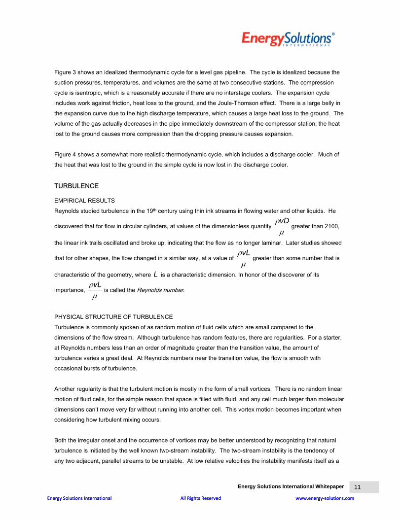
EMPIRICAL RESULTS Reynolds studied turbulence in the 19th century using thin ink streams in flowing water and other liquids. He

discovered that for flow in circular cylinders, at values of the dimensionless quantity µρvD

greater than 2100,

the linear ink trails oscillated and broke up, indicating that the flow as no longer laminar. Later studies showed

that for other shapes, the flow changed in a similar way, at a value of µρvL

greater than some number that is

characteristic of the geometry, where is a characteristic dimension. In honor of the discoverer of its

importance,

L

µρvL

is called the Reynolds number.

PHYSICAL STRUCTURE OF TURBULENCE Turbulence is commonly spoken of as random motion of fluid cells which are small compared to the dimensions of the flow stream. Although turbulence has random features, there are regularities. For a starter, at Reynolds numbers less than an order of magnitude greater than the transition value, the amount of turbulence varies a great deal. At Reynolds numbers near the transition value, the flow is smooth with occasional bursts of turbulence. Another regularity is that the turbulent motion is mostly in the form of small vortices. There is no random linear motion of fluid cells, for the simple reason that space is filled with fluid, and any cell much larger than molecular dimensions can’t move very far without running into another cell. This vortex motion becomes important when considering how turbulent mixing occurs. Both the irregular onset and the occurrence of vortices may be better understood by recognizing that natural turbulence is initiated by the well known two-stream instability. The two-stream instability is the tendency of any two adjacent, parallel streams to be unstable. At low relative velocities the instability manifests itself as a


11



continuous wave at the interface. These waves can be seen on water, sometimes in cloud formations, and in waving flags. Even though a flag is not made of a fluid, the freedom of the cloth to move in a lateral direction permits waves to travel down the flag. (The restriction on motion in the wind direction produces the difference in velocity driving the instability.) Even the onset of turbulence can be seen in a flag’s motion. If the wind velocity is high enough, the end of the flag will curl, in an attempt to move in a vortex. Of course, vortex rotation cannot be completed because of the constraint of the cloth, but the continued attempts eventually tatter the end of the flag. LAMINAR-TURBULENT TRANSITION The quantitative details of the laminar turbulent transition are not well understood. Empirical relations are available that are reasonably good; at Reynolds numbers near the laminar region the results are uncertain. If a pipeline is operated very quietly with a smooth inlet, then it is possible to have laminar flow well above the transition Reynolds number. The laminar flow is unstable, and may be triggered into turbulence by small disturbances.

DRAG REDUCTION

Over about the last fifty years, a variety of techniques for reducing frictional drag in pipeline flow have been found. The two main methods that have seen actual use in the field are solutions of polymers and lubricated flows. Before getting into the complex mechanisms behind these two forms of drag reduction, it is helpful to examine the action of laminar boundary layers in more detail. ROLE OF LAMINAR BOUNDARY LAYER The onset of turbulence occurs when turbulent eddies become more effective at resisting shear motion than viscosity. Eddies resist shear by transporting faster-moving fluid across the stream and dumping it among slower-moving fluid and vice versa. This procedure can dissipate shear motion in direct proportion to: 1. How far across the flow fluid is moved (the eddy size) and

2. How quickly fluid is carried from one region to another (the eddy velocity).

The size of the largest eddies is comparable to the diameter of the pipe, and the eddy velocity is proportional to the flow velocity. The product of eddy size and eddy velocity gives an effective "eddy viscosity" analogous to the kinematic viscosity of a gas caused by thermal (Brownian) motion, which is proportional to the mean free path of the molecules (which is how far a typical molecule is carried across the flow by thermal motion) and the thermal velocity of the molecules (which is how quickly molecules are carried across the flow). The Reynolds number of a flow is, within a constant, the ratio of the eddy viscosity to the kinematic viscosity. Of course, eddies cannot penetrate the pipe wall. This means that very close to the wall, the eddy viscosity is reduced because eddies can't carry fluid as far across the stream. The Reynolds number of flow close to the


12



wall is thus less than the mid-stream Reynolds number, and approaches zero at the surface of the wall. At low Reynolds numbers flow is laminar, so there is always a boundary layer of laminar flow at the wall. The wall of a pipe is never perfectly smooth. Pipe flow occurs with much less drag if the wall irregularities are entirely contained within the laminar boundary layer ("smooth-pipe turbulent flow") than if they extend out of the boundary layer and interact with the turbulent eddies ("rough-pipe turbulent flow"). The most common modern method of pipeline drag reduction, which is the use of dilute solutions of very long polymers, is based on reducing the interaction of the wall irregularities with the turbulent vortices in rough-pipe turbulent flow. LONG-CHAIN POLYMERS In 1946, while investigating mechanisms for the breakdown of solutions of very-high-molecular-weight polymers in turbulent flow, Toms [Reference 3] noticed a startling effect: as the concentration of the heavy, viscous polymer increased, the frictional drag actually declined. This was the opposite of the expected effect, which is that adding a highly viscous component to a flowing fluid increases the viscosity and makes the frictional drag worse. The cause of this behavior, which is known as the Toms phenomenon, is still not perfectly understood. It only occurs during rough-pipe flow, when the wall roughness extends above the laminar boundary layer; it's accompanied by the creation of a second boundary layer on top of the laminar sub-layer, called the "elastic layer". In this elastic layer, some mechanisms for energy transfer between eddies of different scales are suppressed. This has the effect of reducing the drag from turbulent eddies interacting with wall roughness. As the concentration of drag reducer increases, the elastic layer grows thicker until eventually it fills the pipe (at which point further addition of drag reducer has no effect.) Strangely, the drag reduction does keep increasing even after the thickness of the elastic layer has exceeded the characteristic scale of the roughness. Polymer drag reducer is now commercially available for use in both crude and product pipelines. In the last decade, another type of drag reducer based on cationic surfactants has been found which acts in a similar manner. The polymer drag reducers become less effective as the long molecules (often having molecular weights in the millions) are broken up in the turbulence of the flow and as they go through pumps. Surfactant drag reducers are made of much smaller molecules that form weakly bound (compared to molecular bonds) structures which spontaneously re-form after being disrupted in a pump, so for the first time they allow this sort of drag reduction in circulating flows LONGITUDINAL GROOVES Longitudinal grooves also reduce drag by eliminating the smaller turbulent eddies. Another way of looking at the effect is to consider the grooves as small pipes themselves. The Reynolds number is very low because of the small diameter, and so the flow in the groove is laminar even though the flow in the main body of the pipe is turbulent. The interaction of the flow with the surface roughness takes place largely within the groove.


13



OIL AND WATER The pressure added by pumps to fluid flowing in a pipeline is balanced by the wall-shear stresses in the fluid. If there are two immiscible fluids flowing together with very different viscosities (e.g. water and a heavy crude oil) then if the water can somehow be induced to flow in the high-shear outer region of the pipe and the crude in the inner region, the required pumping pressures are just what would be required to pump pure water at the same total flow rate. This can be better understood by noting that the high-viscosity core of oil is much more resistant to shears that the annulus of water, and so the necessary shear implied by the fact that the water exactly at the boundary of the pipe must be still (as was discussed above) will occur almost entirely inside the annulus of water, with the core of oil moving almost like a solid floating in the flowing water. As it happens, a mixture of oil and water with oil that is either heavier or lighter than the water naturally arranges itself into a core of oil and an annulus of water. This also occurs if the fluid starts out as an emulsion, in which case the core contains an emulsion of with higher oil content and the annulus pure water. The mechanism by which the core forms and “levitates”, that is, moves off the wall to the center of the pipe, is not perfectly understood.

CONCLUSIONS

We have reviewed the physics of pipeline flow from the microscopic viewpoint of the forces and energy flows in a fluid element, and from a macroscopic viewpoint of the overall energy flow. The physics is understood well enough that it is possible to produce accurate simulations based on fundamental laws, with the caveat that there may be errors in special situations, such as the laminar-turbulent transition zones due to the effects of instabilities or of influences not quantifiable or even not fully defined.


14



REFERENCES

1. Modisette, Jerry L. Equations of State PSIG 2000

2. Modisette, Jason P. Pipeline Thermal Models PSIG 2002

3. Toms, B. A. On Early Experiments on Drag Reduction in Polymers, PHYSICS OF FLUIDS (1977) 20, 10,11,S3-S5.


15



FIGURES

Figure 1 – Forces on a Cross-section of Fluid


16



Figure 2 – Force Diagram for a Point Fluid Element


17



Figure 3 – Pipeline Thermodynamic Cycle

Cycle

Pipeline Thermodynamic Cycle

300

400

500

600

700

800

900

1000

1100

700 900 1100 1300 1500 1700 1900

Volume, cu ft/mole

Pres

sure

, psi

a

CompressionExpansion


18



Figure 4 – Pipeline Thermodynamic Cycle with Discharge Cooling

Pipeline Thermodynamic Cycle - w. Discharge Cooling

300

400

500

600

700

800

900

1000

1100

700 1200 1700 2200

Volume, cu ft/mole

Pres

sure

, psi

a

CompressionExpansionCooling


19


jason modisette, energy solutions jerry modisette, consultant … · 2017-06-25 · jerry...

Documents