jay james j. o'brien

The Effects of El Nino on Rainfall and Firein Florida

Catherine Stephens Jones, Jay F. Shriver andJames J. O'Brien

El Nino is only one phase of a larger ocean-atmospherecirculation termed the Southern Oscillation (SO). A complementaryphase of EINino known as La Nina or El Viejo constitutes the otherphase of the SO. The SO is the dominant mode of interannualvariability in the tropics. Several parameters exhibit interannualvariability and all have a center region in which the SO accounts forthe major portion of the parameter's variance (Philander 1990).Surface pressure, sea surface temperatures and convective zones arcsuch parameters. Interannual fluctuations in the sea surface ternperature (SST) are noted to be a maximum between 10 degrees northand south in the central and eastern equatorial Pacific.

An El Nino event, or warm anomaly, is referred to as a low S().Meanwhile. a high SO, known also as a cold anomaly, constitutes LaNina. This phase is characterized by lower than normal SST due tointense trade winds which upwell cold water to the surface in theeastern tropical Pacific (Philander 1985). The Intertropical Convergence Zone (ITCZ) and South Pacific Convergence Zone (SPCZ)diverge on either side of the equator and less rainfall is observedover equatorial South America and the eastern Pacific. This coldanomaly is a relatively new discovery and the specific years of LaNma are not agreed upon. On the other hand, general criteria existfor warm anomalies and these events are agreed upon. For thepurpose of this study, the classification of warm and cold anomaliesis taken from Yuri Volkov and Boris Kalashnikov's list (1990) andfrom the Galapagos Islands sea level data since sea level data is

Ms. Jones and Mr. Shriver are graduates of the Department of Meteorology, FloridaState University, Dr. O'Brien is Professor of Meteorology and Head of the university'sCenter for Oceanic and Atmospheric Prediction, Tallahassee, FL 32306

55

Jones, Shriver, and O'Brien Effects of El Nino

directly related to temperature anomalies. Warm temperatureanomalies are indicative of high sea level pressures and conversely,cold anomalies indicate low sea level pressure. By this classification,warm anomalies exist when sea surface temperature and precipitation increase in the eastern equatorial Pacific, sea surface leveldifferences between the eastern and western equatorial Pacificdecreases, and the zonal component of the southern trade windsdecreases in the Pacific.

The term EI Nino originally implied an annual weak warmcurrent running southward annually off the coast of Ecuador.Currently the term is associated with extended periods of unusuallywarm SST's occurring periodically off the western coast of SouthAmerica and in the central and eastern tropical Pacific. These eventsoccur approximately every three to seven years off the western coastof Peru and Ecuador and exhibit temperatures several degrees abovenormal (O'Brien 1987). Major ocean currents regulate the transportof heat. Busalacchi and O'Brien (1980) investigated the seasonalresponse to surface currents in the tropical Pacific. Similarly, Wrytki(1975) described the seasonal traits of the equatorial currents in thetropics. A basic comprehension of the seasonal variations of equatorial currents, specifically in the eastern tropical Pacific, is essential tobetter understand EI Nino events which involve intense disturbances of those seasonal variations.

As stated previously, ocean heating plays a significant role in thegeneration of warm anomalies referred to as EI Nino. The westernequatorial Pacific Ocean is the source of an EI Nino event. In thePacific Ocean the ITCZ, the SPCZ and the convective zone across themaritime continent in the western tropical Pacific are importantregions of heating (Philander 1985). During an El Nino event, theITCZ and the SPCZ are displaced toward the equator. Philanderclaims SST's influence the movement of the convergence zones. Thesummer seaSOI1 of the western Pacific in the Northern Hemisphere,where SST's are the warmest, is witness to a strong ITCZ while thewinter season in the Northern Hemisphere (summer in the SouthernHemisphere) experiences a strong influence of the SPCZ and a weakITCZ. The ITCZ is at the southernmost position in March and Apriland at the northernmost position between August and September atapproximately 10 - 15 degrees of latitude north. The occurrence ofwarm anomalies is most favorable early in the year, when the rTCZis in its southern most position and the SST's are generally at aseasonal maximum. Even small variations in the position of theseconvergent zones can heavily affect the rainfall in certain areas.

56

The Florida Geographer

Likewise, the convective zones around equatorial Africa and Centraland South America, again under the influence of SST, somewhatcontrol rainfall patterns. Given high SST's, warm, moist air rises andcreates greater convection around the equator which produces morerainfall.

Another trait of El Nino also related to the SST is the fluctuationof the trade winds. A relationship between equatorial ocean currentsand the trade winds is important when forecasting El Nino events.Most knowledge of this correlation is obtained from dynamic heightand sea level analyses within the tropics (Busalacchi and O'Brien1985). l\ large change in atmospheric pressure between the easternsubtropical Pacific and the maritime lands of Australia and Indonesia generate easterly trade winds (McPhaden and Picaut 1990).Warm surface waters are generally related to a lessening of the tradewinds. Westerly wind stress anomalies, caused by the relaxation ofthe trades in the central and eastern equatorial Pacific, generateKelvin waves (Graham and White 1988). These Kelvin wavesreinforce the SST anomaly in this region by decreasing the depth(thickness) or the warm water in the western tropical Pacific and byincreasing the depth in the eastern tropical Pacific. A clash of thetrades over the warm water produces a line of heavy convection andclouds, thereby influencing precipitation patterns.

Thus, an EI Nino event results from warm SST anomalies. Thesewarm SST's are continuous for at least four months and at three ormore coastal stations. El Nino events also result from a relaxation ofthe trade winds in the central and eastern tropical Pacific. Thisrelaxation leads to the convergence of the ITCZ and the SPCZaround the equator. Low surface pressure over the southeasterntropical Pacific and large amounts of precipitation are also noticedduring an El Nino event.

For many years, El Nino was viewed only as a destructiveoccurrence (Philander 1990). However, this research indicates an ElNifio event actually brings relief to Florida while its counterpart, anEI Viejo, or La Nina, event yields negative results in Florida. Theauthors will examine the relationship between the amount ofrainfall in an EI Nino event and the number of acres burned acrossFlorida. Such a correlation could help prevent the destruction ofland by better predicting the dryness or wetness of a season.

In addition to fire management, a correlation could be of ecological importance. Fires are a cause of economic loss and also of basicecological processes which are likely to change with future climates.The impact of local ecological processes in ecosystems could dimin-

57


f'

ish if a connection between fire and climate is substantiated sincesome systems are regulated by fire frequency and intensity. Arelationship between fire and climate could also help predict futurevegetation (Sweetnam and Betancourt 1990).

Douglas and Englehart (1981) concluded heavy rainfall events inthe equatorial Pacific during autumn are frequently followed by wetwinters in the southern United States. They also concluded thatheavy precipitation in Florida is the result of a strong low-latitudeflow across North America and an increase in frontal activity in theGulf of Mexico. Meteorologists refer to this strong flow as thesubtropicaJ jet stream. When the subtropical jet stream is shifted, alow pressure center is located over Mexico and the convective zoneis shifted to the Gulf of Mexico, and includes Cull coastal states ofthe United States. Normally, a high pressure center sits off thewestern coast of Mexico and California, keeping Florida drier in thewinter.

Sweetnam and Betancourt (1990) conducted a similar study ofthe southwestern United States using fire data from 1905 to 1989.Research showed that large areas of burn after dry springs wererelated to the high phase of the Southern Oscillation (SO), acceptedas being associated with the La Nina phase of the SO. Meanwhile,small areas of burn after wet springs were associated with El Ninoevents. Sweetnam and Betancourt (1990) concluded the relationshipto be the strongest during the extreme phases of the SC).

Brenner (1990) examined monthly wildfires in Florida and theirrelationship to anomalous SSTs and sea level pressures. A simplestatistical analysis confirms such a relationship. Early personalcontact by Brenner with the authors led to this pi-lper. In this study,empirical orthogonal function analysis is applied to fire data fromeach Florida county and rainfall data in 22 cities in order to determine the variance of the spatial and temporal patterns in the data.The significant, repetitive patterns are compared to the sea levelpattern off the Galapagos Island which is indicative of El Ninoevents.

Method

Empirrcal orthogonal function analysis (E()F) is a purely statistical method of examining data and is used frequently in handlingmeteorological and climatic data (Preisendorfer 1988). Physicalinterpretation of the results are necessary. An empirical orthogonal

58


function is a linear function dependent in this case on space (the 67counties in Florida) and time (108 months of fire data from the years(1981-1989). One linear separable function of the data set is:

D(s,t) =(;(s)f1(t)Where G(s) represents the spatial function and H(t) represents thetemporal function. The first principal component is the linearfunction which has the maximum possible variance. The secondprincipal component is the linear function with the maximumvariance subject to being uncorrelated with the first principalcomponent and so forth (Joliffe 1981). The total data set is definedby the data matrix (0):

o =(dsT)Where for example, s ranges from 1 to 67, representing the 67counties throughout Florida, and t ranges from 1 to 108, representing the number of the month of data acquired. A space by spacecorrelation matrix (C) is formed by collapsing the initial temporalcomponents of the original function:

In order to calculate the variance, the correlation matrix is dividedby the number of points (N). A twelve month moving average waslater carried out to filter large twelve month variances and to isolatesignificant and repetitive modes. Only 97 temporal componentsremain after this statistical filter. The diagonal (trace) of the newcorrelation matrix now represents the variance for each of the 67counties in Florida. The remaining values in the matrix represent thesample covariances for the various counties.

The sum of the diagonal (the trace of C) is equal to the sum of theeigenvalues which is also equal to the sum of the squared variances(See Kim). Because C is symmetric, all of the values are real. Startingwith the largest eigenvalue, the eigenvalue is divided by the trace ofC to determine the percentage of total variance in the eigenvectorassociated with the maximum eigenvalue. The usefulness of thisstatistical method depends on how much of the total variance isaccounted for by the first few eigenvalues (Moore 1974).

Eigenvalue coefficients are extracted from the two most significant modes and the temporal components were calculated (Figures 3and 4). The 67 eigenvector coefficients are likewise extracted from

59

Jones, Shriver, and O'Brien Effects of £1 Nino

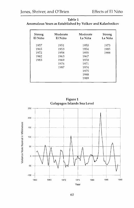
Table 1Anomalous Years as Established by Volkov and Kalashnikov

Strong Moderate Moderate StrongEl Nino £1 Nino La Nina La Nina

1957 1951 1950 19731965 1953 1954 19851972 1958 1955 19881982 1963 19671983 1969 1970

1976 19711987 1974

197519881989

Figure 1Galapagos Islands Sea Level

c

C1jEozE£Q)oc::::(0

~

-100 -l-----+-----------IL-------+------+--------f-------j

1960 1965 1970

60

1975

Year

1980 1985 1990


Figure 2Variance from Normal Monthly Rainfall

-10 -l- -----r----- -- 1- ------1----- --r----- -T-1950 1955 1960 1965 1970 1975

---r------ ---T-1980 1985 1990

U)

a>CD.~CQ)

0.~

roE0z 0E~~ -2cn::l

~-4

-6 -1------- -1---------1----

1950 1955 1960

6---,---------···

--- r------- ------ -1 ------r------ ----T

1965 1970 1975 1980 1985 1990

2

o

-2

-4

-6

1950

-----1---------- -- ----------r---1960 1965 1970

61

---r-------- --19"75 1980 1990


the two most significant modes. and are plotted to form the spatialcomponents (Figure 5 and 6). Eighty-eight percent of the variancewas detected within these two significant modes.

Rotational EOF analysis often follows the above process. Rotational analysis is based on a linear rotation around the axes. However, unrotated solutions are easier to extract maximal variance fromthe data; they have spatial and temporal orthogonality, and are alsoinsensitive to the number of principal components (Richman 1986)The method of unrotated EOF's is good for situations in which puredata reduction is desired, but the method may hinder the ability toisolate individual modes of variation. Rotational analysis was notperformed as rotation of the principal components would havealtered the pattern very little.

The same method was applied to the monthly rainfall data. Thespatial components are the 22 sites across Florida while the temporal components are 360 months of rainfall totals. The first twosignificant modes comprised 55 percent of the variance as comparedto 88 percent in the fire data.

Figure 3Empirical Orthogonal Function Analysis of Fire Data

for Time Series 1

! 000:: ]~ --_.-I=-=I-=-~r~--------[~- -.i 0015t----I~---~-~--+---.----l- --~f 001 -t-----T--- -t----l------------- f- -- -1i 0005 -------i--- ~--t-- -- ---I

<5z 0--

E I,g I

§ -0005 ~--~ , I I I I i

-0.01 +---- -.-------..----1--- ------- .. -- ------+--- ..---- ----- .. -1------------------1-----11980 1982 1984 1986 1988 1990

62

Percentage of TotalCounty Area

0 ··004 - 0

o 0- .004

C .004 - .0 10

• .0 10- .030

• Greater than .030


Data

The Galapagos sea level data were measured by several gaugesput together by Klau s Wyrtki. The data encompasses the year 19591989. To h ighlight the interannual variability, a 12 month movingaverage was used . A comparison of Wyrtki's data and the list of coldand w arm anomalies as classified by Volkov and Kalashnikov (Table1) helps determine a relationship between the anomalous years andthe Florida data .

The initial data set to be examined which included the number offires and the number of acres burned in each county for a period of108 months was provided by Florida's Division of Forestry. 111edata were normalized by county acreage so that the county size did

Figure 4Variance from Normal of Total County Area Burned

for Time Series 1

, ,-- ···- ···-----·----- -..- ·-·- -- -- --·..·--- ·------ --·1

(--( -T--l---r-;-r'-) I<> 1.. J.-, \. ~'--rt--.5?1-r- -- '.-"--""---'- IJ ' ~ - - , ' -"',J:;,~ r t:: . xt -:

" ~~;-~, ~ - . I

'\{ I

I

L... . ._._. . .

63


not bias the sta tistics, Rainfall data were obtained through the stateclimatologist for a 30-year period. Twenty -two sites were selectedas an appropriate representation of the various regions in the state.

First, a mean plot of the total number of acres burned over the108 months was constructed. This figure indicated areas of littleburn in 1983 and in 1987, years of known EI Nino events. Meanwhile, data for 1985 indicated an above normal fire year and data for1989 showed a record year for acres being burned. These are years ofanti-EI Nino events according to the table from Volkov andKalashnikov. The Galapagos sea level data (Figure 1) also indicatesthese years to be anti-El NU10 years.

Anomalies of monthly rainfall plots of three particular cities,Apalachicola, Tampa, and Tarniami (Figure 2) are very similar to theGalapagos data. A11 three of the sites show a marked increase inrainfall during the years of strong El Nines -1957/1965/1982 and1983. Moreover, the strong EI Viejo years of 1973 and 1985 arerepresented by below normal rainfall in each of these cities. Thus,the data appear believable on first examination.

Figure 5Empirical Orthogonal Function Analysis of Fire Data

for Time Series 2

I-_._---------1---- --------'--------j

I-----t----- -,._-- -,---- t -

I IL------ -t-- '

I . +I

--------,----- --r----- -----!

----- -----------1

i

-------.,"---{----_---- 11 --

I---1'--- -1---------------

!

o

0.004 --,------------ ----

0.002

0.006 --

0.010 -

Q)u

~ -0.002

~

CDQ.l

<>- 0.008C:Joo(U

~oQ)

0>roCQ)t::'Q)

CL

.SroEozEE

-0004

1980 1982 1984 1986

i

1990

64


Although the first two rainfall eigenmodes represent about onehalf the variance, it is sufficient to show the monthly totals ofrainfall for these three cities . In essence, a combination of the spatialand temporal components is being displayed. The number of firesand acres burned is a consequence of the amount of rainfall received. By showing the eigenmodes of the fire data, readers shouldrealize these patterns are indicative of the rainfall data as well.

Together, the first two statistical modes of fire data account for 88percent of the variance. At first glance, a relationship appearsevident. The first significant temporal mode (Figure 3) accounts for72.62 percent of the variance in the data and is closely related to theGalapagos Island sea level plot. Peaks in the sea level correspond to

Figure 6Variance from Normal of Total County Area Burned

for Time Series 2

Percentage of Total County Area

D - 004 - 0

D 0-004

l[TI .004 - .010

• .010-.030

• Greater than .030

.,." .

65


El Nino years (particularly 1982-83 and 1987), which correspond to alow number of acres burned.

Meanwhile, the most notable valleys in the sea level plot (1985and 1989) correspond to the peaks in the first time series. Coldanomalies with large numbers of acres burned occurred in theseyears. The spatial mode must be examined with the temporal modein order to yield an overall picture. The product of the spatial andtemporal modes produces the percentage the county burned. Thefirst spatial pattern (Figure 6) shows a strong influence in southernFlorida. The southwestern tip and two northeastern counties exhibitanomalous values relative to the rest of the pattern.

The second time series (Figure 4), which accounts for only 16.75percent of the variance, also exhibits a peak in 1985 and two valleysin 1983 and 1987. However, another peak is noticeable in 1981 and avalley in 1989.

The first temporal mode accounts mostly for the EI Viejo and thesevere burning in 1989. This mode accounts only slightly for the EIViejo in 1985. The second temporal mode combined with the firstmode shows the influence of a strong El Nino period in 1982-83 anda strong El Viejo in 1985. Since the variance percentages of the 67modes should sum to one, Saine compensation is likely to beoccurring in this second mode. For example, a large peak is observedin mode 1 in 1989, while a large valley is noticed in mode 2.

Examination of the second spatial mode (Figure 6) also indicatesa relationship of acres burned to El Nino events. In this mode centralFlorida experiences the most burning while very little burning isobserved in the Panhandle. Combined with the second temporalmode, twelve percent of each of the counties in central Floridawhich exhibited the strongest influence are burned. Again, theextreme southwestern and a couple of northeastern counties areoutliers to the pattern. These counties are mostly unincorporated.For example, the southwestern region of Florida consists mainly ofthe Everglades National Park and the Big Cypress National Preserve. The northeastern counties are comprised mainly of forestsand wetlands, including part of the Okefenokee National WildlifeRefuge.

When examining the temporal and spatial modes together, thefirst mode represents the 1989 El Viejo which is most apparentacross southern Florida with some of the 1985 EI Viejo noticeable inthe northeast portion of Florida. The second mode represents the1985 El Viejo across much of central florida and in a few counties inthe Panhandle. Southern and central Florida experienced the most

66

burning while the Panhandle of Florida experienced little burningduring both of these events in 1985 and in 1989. Baker and Monroecounties are anomalous in both modes. However, the overall patternis strong enough to conclude a definite relationship exists betweenan E1 Nino/El Viejo event and the numbers of acres burned.

Possible anomalies in the aforementioned areas In,ly be causedby the location. More moisture along the Panhandle counties ofFlorida from the Gulf of Mexico could prevent fires in these counties.

Summary

Statistical analysis of rainfall and fire data across Florida indicates two recurring spatial and temporal patterns which account for88 percent of the variance in the number of acres burned per yearand 55 percent of the variance in the amount of rainfall, In a strongEI Nino phase, warm SST's exist off the coast of Ecuador whileFlorida experiences a cool, wet winter in which fewer acres areburned. In contrast, more acres are burned during an El Viejo phasewhich is related to warm, dry winters in Florida. This relationship ismost prevalent during the extreme phases of the Southern Oscillation. Large anomalies existed in the years 1983, 1985,1987, and 1989in which strong or moderate phases of the S() occurred. The warmEl Nino anomalies in 1983 and 1987 produced very little burningand extremely wet winters. Cool E1 Viejo anomalies in 1985 and 1989produced a record number of acres burned in Florida as a result oflittle rainfall. Based on the two spatial patterns of the fire data,southern Florida exhibits the strongest relationship to EI NinolE1Viejo events while the western panhandle indicates very littlecorrelation. Spatially, northern Florida, particularly the Panhandle,received more rainfall than the other areas. However, all regionsshowed a significant increase in rainfall during the EI Nino years.

Although the number of fires and acres burned are a result of theamount of rainfall, statistical analysis shows that the rainfall data isa good indicator of El Nino events, while the fire data is moresignificant to the E1 Viejo events.

The fire data do not cover an extensive period of time since priorto 1980 records were listed by districts. Analysis may change with alonger time series. However, the results are conclusive for the nineyear period analyzed with rainfall and fire data. A relationship existsamong the amount of rainfall received, the number of acres burnedin Florida, and E1 Nino events. Therefore, better prediction of such

67

]011es, Shriver, and O'Brien Effects of El Nino

events will help prevent the destruction of wildlife areas andnational fores ts.

References

Barnett, T., N., Graham, M. Cane, S. Zebiak, S. Dolan, J. O'Brien, andD. Legler (1988) "On the Prediction of the El Nino of 1986-1987,"Science 241: 192-196.

Brenner, James (1991) "Southern Oscillation Anomalies and TheirRelationship to Wildfire Activities in Florida," lnternationa! journal ofWildland Fire 1: 73-78.

Douglas, Arthur V., and Phillip Englehart (1981) "On a StatisticalRelationship Between Autumn Rainfall in the Central Equatorial'Pacific and Subsequent Winter Precipitation in Florida," Monthly-Weather Reoieio 109: 2377-2382.

Graham, Nicholas E., and Warren B. White (1988) "The El NU10Cycle - A Natural Oscillator of the Pacific Ocean-AtmosphereSystem," Science 240: 1293-1301.

Inoue, Masarnichi, and James J. O'Brien (1987) "Interannual Variability in the Tropical Pacific for the Period 1979-1982," journal ofGeophysical Research 92: 11671-11679.

Jolliffe, Ian T. (1986) Principal Component Analysis. New York:Springer -Verlag.

Johnson, Mark A'I and James O'Brien (1990) "The Northeast PacificOcean Response to the 1982-83 £1 Nino," journal of GeophysicalResearch 95: 7155-7166.

McPhaden, M.J., and J.Picaut (1990) /lEI Nino-Southern OscillationDisplacements of the Western Equatorial Pacific Warrn Pool." Science250: 1385-1388.

Moore, Dennis (1974) "Ernp ir ical Orthogonal Functions - A NonStatistical View," Mode 1Jot Line Ncui» No. 67.

lY13rien, James J. (19H7) "Using Supercomputers to Understand andForecast El Nino," ETA SystenlS Publication Vol 4, NO.2.

68


Philander, S.G. (1985) "El Nino and La Nina," Journal of the Atmospheric Sciences 42: 2652-2662.

Philander, S.G. (1990) EI Nino, LaNina and the Southern Oscillation.San Diego: Academic Press.

Preisendorfer, Rudolph W. (1988) Principal Component Analysis inMeteorology and Oceanography. New York: Elsevier Science PublishingCo. pp. 1-89.

Richman, Michael B. (1986) "Rotation of Principal Components,"Journal of Clilnatology 6: 293-335.

Sweetnam, Thomas W., and Julio Betancourt (1990) "Fire-SouthernOscillation Relations in the Southwestern United States," Science249: 1017-1020.

Tolmazin, David (1985) Elementsof Dynarnic Oceanography. Boston:Allen and Unwin.

Wyrtki K. (1975) "El Nino. The Dynamic Response of the EquatorialPacific Ocean to Atmospheric Forcing." Journal of Physical Oceanography 5: 572-584.

Zebiak, Stephen E., and Mark A. Cane (1987) "A Model E1NmoSouthern Oscillation." Monthly Weather Reoieto 115: 2262-2278.

Acknowledgments

This research was supported by NASA grants NGT 50653, NGT30056, and NAGW-985. Without this support, this research wouldhave been a difficult task. Research grants from the Physical Oceanography Section and Climate Group of the National Science Foundation supported James O'Brien. We thank Jim Brenner for the firedata, Klaus Wyrtki, University of Hawaii, for the sea-level data, andTom Gleeson, Florida State University Climate Center, for therainfall datao

69

digitstaff

Text Box

jay james j. o'brien

Documents