1

On the integration of m-dimensional expectation operators

James D. Turner1 and Ahmad Bani Younes2 Submitted to:

Jer-Nan Juang Astrodynamics Symposium

Texas A&M University, College Station, TX, June 24-26, 2012

Abstract

Multivariable estimation theory has as part of its foundation the need for computing expectation values

of state variables. A common assumption is that the governing statistics are governed by Gaussian

random variables. It is well known that odd ordered expectation values vanish. Several approaches

have been proposed for computing 4th, 6th, 8th, and higher order expectation values‎1-‎4. For example,

Isserlis’ or Wick’s theorems provide a formula that theoretically allows one to compute higher-order

moments of a multivariate normal distribution in terms of its covariance matrix. In 1918 Isserlis proved

the following theorem by mathematical induction, given: 1 2, , nx x is a zero mean multivariate

normal random vector, then

1 2 2

1 2 2 1 0

n i j

n

E x x x E x x

E x x x

(1)

where the notation means summing over all distinct ways of partitioning 1 2, , nx x into pairs;

yielding

12 1 !! 2 1 !/ 2 1 ! 1*3*5*7*...*(2 1)nn n n n

terms in the sum. Isserlis provided explicit formulas for computing the expectation operators through

4th order. The main contribution of this paper is the presentation of a symbolic computational method

for generating closed-form solutions for arbitrary order expectation operators using only elementary

calculus tools. Closed –form solutions are provided for two cases: (1) non-zero mean, and (2) zero mean

applications. The symbolic results are validated by introducing an n-dimensional spherical coordinate

transformation, where the radial part of the integral and all of the (n-1)-dimensional solid angle tensor

integrals are evaluated in closed-form. The analytical formulations are useful for two significant

applications: (1) statistical moment propagation for nonlinear models using tensor state transition series

1 Research Professor, Aerospace Engineering, Texas A&M University, College Station, Texas,

turner@aero.tamu.edu, Fellow AAS, Associate Fellow AIAA 2 PhD Candidate, Aerospace Engineering, Texas A&M University, College Station, Texas, olalahmad@gmail.com

(Preprint) AAS 12-641

2

expansion methods, and (2) sum of Gaussians approximations for approximating probability distribution

functions.

Multivariate normal random vector probability density function: The goal of this analysis is to

analytically integrate tensor-based expectation functions of m-dimensional multivariate normal

distributions defined by

1 /21/2/2

0, 2tx R xm

xN R R e

(2)

where R denotes the covariance matrix and the mean is assumed to vanish (see APPENDIX C for the

case where the mean does not vanish). The standard probability modeling assumption is that the

distribution of Eq. (2) is normalized as follows

1 /21/2/2

1 22 1;tx R xm m m

mR e dx dx dx dx dx

(3)

where the integral is assumed to be evaluated over the m-dimension volume. The 1st order expectation

operator is given by

1 /21/2/2

2 0tx R xm mE R e dx

x x (4)

and the 2nd order expectation operator is given by

1 /21/2/2

2tx R xm mE R e dx R

xx xx (5)

Generalized Integral Expectation Calculations: New applications in nonlinear uncertainty modeling

methods are creating a need for computing additional higher-order expectation integrals of the form:

1

1

1

/21/2/2

/21/2/2

/21/2/2

2

2

2

t

t

t

x R xm m

x R xm m

x R xm m

E R e dx

E R e dx

E R e dx

xxxx xxxx

xxxxxx xxxxxx

xxxxxxxx xxxxxxxx

(6)

The main contribution of this paper is the development of two independent methods for validating

closed-form solution for the tensor expectation operators listed above. The first method exploits

computer-aided algebra tools for developing closed-form expressions for the tensor elements of

expectation operators, by differentiating a known integral w.r.t. a parameter. The second method

introducing a change of variables that replaces the original state space vector with an m-dimension

spherical coordinate transformation, where the both the radial and angular parts of the integrals are

evaluated in closed-form. Numerical examples are presented that validate the proposed solution

3

approaches. These ideas are generalized in the APPENDIX C to handle the case that the mean value is

non-zero.

A. Symbolic Algorithm

Closed-form solutions are obtained by invoking a standard trick from calculus; namely, computing

derivatives of integrals with respect to parameters to create related integrals of interest. These ideas

are first developed for the scalar case and then generalized for the matrix-vector case. To this end,

assume that that one has available the following scalar Gaussian integral:

2

2( ) 4

s

ax sx aI s e dx ea

(7)

First we transform the integral to get the required functional dependence for the Gaussian probability

integral definition. To this end, let a = 1/(2r), yielding

2

2( /(2 ) ) 22s r

x r sxI s e dx re

Normalizing the integral by 12 r

and evaluating the limit s => 0, leads to

2( /(2 ))

0

1 1limit 1

2 2

x r

s

I s e dxr r

which recovers the standard Gaussian integral normalization. Two addition facts must be true for Eq. (7)

to be useful. First, the 1st moment integral must vanish. Second, the 2nd moment integral must equal

the covariance. The first moment integral calculation is confirmed by taking the first derivative of the

Eq. (7) w.r.t. s, and evaluating the limit as s =>0,yielding

2

2

2

2

( /(2 ) ) 3/2 2

( /(2 )) 1/2 2

00

2

1 1limit 0

2 2

s r

x r sx

s r

x r

ss

dI sxe dx r se

ds

dI sxe dx r se

dsr r

which is the expected result. The second moment calculation is confirmed by taking two derivatives of

Eq. (7) w.r.t s, and evaluating the limit as s=>0, yielding

4

2

2

2

2

2 2

2 2 22 ( /(2 ) )

2 2

2

2 ( /(2 )) 5/2 2 3/2 22

0

3/2 2 2 2

0

2

1 1 2limit

2 2 2

s r

x r sx

s r

x r

s

s r s r

s

d I s d ex e dx r

ds ds

d I sx e dx r s r e

dsr r r

r s e re r

which has recovered the expected covariance. As a result, one can conclude that Eq. (7) provides a

useful representation for carrying out Gaussian probability integral calculations. The next section

generalizes these results for the case where x and s denote mx1 vectors, and r denotes an mxm

covariance matrix.

Calculation for the Matrix-Vector Generalization of a Scalar Gaussian Integral: The matrix-vector

generalization of Eq. (7) is assumed to be given by:

1( )t tA mI e dx

x x s x

s (8)

To simplify the quadratic term, one introduces the change of variables 1/2z A x , leading to

1 1/2 1/2( ) ( )t t t tA m mI e dx e A dz

x x s x z z s A z

s (9)

where

1/21/2 1/2dxx A z dx dz A dz A dz

dz

Completing the square one obtains

1/2 1/21/2

1/2 1/2

/41/2 1/2( )

1/2 /4

1/2/2 /4

tt

t t

tt

t

A A Am m

A AA m

m A

I e A dz A e dz

A e e dz

A e

z s/2 z s/2 s sz z s A z

z s/2 z s/2s s

s s

s

(10)

where the final integral is evaluated as product of m uncoupled scalar integrals

1/2 1/2 2/2

1 1

tt

i

m mA A m m m

ii i

e dz e dy e dy

z s/2 z s/2 yy y

5

Comparing Eqs. (3) and (10) it is obvious that 1 1 / 2 2A R A R , leading to

1 1/2 /2 2 /4( )

1/2 1/2/2 /2/2 /2 /2

2

2 2

tt t

t t

m RR 2 m

m mm R R

I e dx R e

R e R e

s sx x/ s x

s s s s

s (11)

Next, one needs to confirm that Eq. (11) generates the expected 0th, 1st, and 2nd order expectation

integrals.

Test the Integral Normalization Condition: Normalizing the integral with the coefficient of Eq. (2) leads

to

1 1/2/2( ) /2

1/2/2 /2

2

2

t t t

t

mR 2 m R

m R

I e dx R e

R I e

x x/ s x s s

s s

s

s

(12)

Evaluating the limit of Eq. (12) as all components of s =>0, one obtains

1/2/2 /2

0 0

limit 2 limittm R

mxmR I e I

s s

s s

s (13)

which recovers the normalization for the multivariable Gaussian distribution function. Higher-order

expectation operators are evaluated by computing partial derivatives w.r.t. scalar components of s and

evaluating the limit of the partial derivative calculation as all of the components of s =>0.

Validate the Mean Calculation: Taking one scalar partial derivatives of Eq. (12) with respect to the ith

component of s, yields

1( ) /21/2/2

1/2/2 /2

2

2

t t t

t

R 2 Rmm

i i i

m R

ij j

I e edx R

s s s

R R s e

x x/ s x s s

s s

s

(14)

taking the limit as all of the components of s =>0 confirms the expected vanishing of the 1st order

expectation integral.

Validate the Covariance Calculation: Taking two scalar partial derivatives of Eq. (12) w.r.t. the ith and jth

components of s, yields

12 2 ( ) 2 /21/2/2

1/2/2 /2

2

2

t t t

t

R 2 Rmm

i j i j i j

m R

ir r jq q ij

I e edx R

s s s s s s

R R s R s R e

x x/ s x s s

s s

s

(15)

6

Multiplying by the normalization for the multivariable Gaussian distribution function leads to

1

21/2 1/2/2 /2 ( ) /22 2

tt tm m R 2 m R

i j ir r jq q ij

i j

IR R x x e dx R s R s R e

s s

x x/ s x s s

s (16)

and evaluating this limit as s=>0, one obtains

1

21/2 1/2/2 /2 ( )

0

limit 2 2tm m R 2 m

i j ij

i j

IR R x x e dx R

s s

x x/

s

s (17)

which analytically recovers the expected covariance matrix for the 2nd order expectation operator.

These results now lay the foundation for computing higher-order expectation operators.

4th and 6th Order Expectation Integrals Calculations: Repeated partial differentiation of the integral of

Eq. (6), w.r.t. the components of s yield the desired integral expectation operator values. A fourth-order

expectation operator is evaluated as follows:

1

41/2 1/2/2 /2 ( )

0

4 /2

0

limit 2 2

limit

t

t

m m R 2 m

i j k l

i j k l

R

i j k l

ij kl ik jl il jk

IR R x x x x e dx

s s s s

e

s s s s

r r r r r r

x x/

s

s s

s

s

(18)

This result was derived by very different statistical arguments by Isserlis‎1 in 1916. Note that this result

implies:

i j k l i j k l i k j l i l j kE x x x x E x x E x x E x x E x x E x x E x x (19)

A sixth-order expectation operator is computed as

1

61/2 1/2/2 /2 ( )

0

6 /2

0

limit 2 2

limit

t

t

m m R 2 m

i j k l m n

i j k l m n

Rs

i j k l m n

ij kl mn ik jl mn il jk mn

ij km ln ik jm ln im jk ln

ij kn lm ik jn lm

IR R x x x x x x e dx

s s s s s s

e

s s s s s s

r r r r r r r r r

r r r r r r r r r

r r r r r r

x x/

s

s

s

s

in jk lm

il jm kn il jn km in jl km

im jn kl in jm kl

r r r

r r r r r r r r r

r r r r r r

(20)

7

In 1918 Isserlis‎2 suggested that this result would be true as defined by the theorem of Eq. (1), but he did

not present any explicit expansion for the tensor components. Note that this result implies the

following

i j k l m n i j k l m n i k j l m n i l j k m n

i j k m l n i k j m l n i m j k l n

i j k n l m i k j n l

E x x x x x x E x x E x x E x x E x x E x x E x x E x x E x x E x x

E x x E x x E x x E x x E x x E x x E x x E x x E x x

E x x E x x E x x E x x E x x E x x

m i n j k l

i l j m k n i l j n k k i n j l k m

i m j n k l i n j m k l

mE x x E x x E x x

E x x E x x E x x E x x E x x E x x E x x E x x E x x

E x x E x x E x x E x x E x x E x x

(21)

Higher-order expectation operators are similarly handled. These results have been obtained by using

the computer-aided algebra system MACYSMA 2.4, where the final symbolic results are converted into

FORTRAN executable outputs. Symbolic calculations have been performed for 4th- through 10th order

expectation integral calculations. Table 1 summaries the complexity of the calculations performed. The

number of terms reported in the 3rd column confirms Isserlis‎2 1918 prediction for the number of terms

encountered (MACYSMA symbolic utilities were used to count the number of terms appearing the

symbolically generated partial derivative expression). The calculations required < 4 secs for computing

1st-10th order calculations, using a decktop PC. The computer-aided symbolic script used for the

MACSYMA calculations is presented in APPENDIX A.

8

Table 1: Computational Complexity of Expectation Operator Partial Derivatives

Partial Derivative Order Number of Terms before Limit*

Number of Terms after Limit^

Number of Terms In each Product

2

i j

I

s s

s 2 1 1

4

i j k l

I

s s s s

s 10 3 2

6

i j k l m n

I

s s s s s s

s 76 15 3

8

i j k l m n p q

I

s s s s s s s s

s 764 105 4

10

i j k l m n p q v w

I

s s s s s s s s s s

s 9496 945 5

* 1

!1 2 ,2 (2 1)!!; ( , )

!( )!

n

k

nSize n C n k k C n r

r n r

^ Size(n) = (2n-1)!!

B. Numerical Methods

To validate the symbolically generated results a numerical method is now developed that transforms the

multi-dimension expectation integrals into a form that can be solved in closed-form by introducing an

m-dimension spherical coordinate transformation. Both the radial and angular parts of the solution are

expressed in closed form in terms of beta and gamma functions.

Change-of-Variables: The evaluation is simplified by transforming the integrals to m-dimension

spherical domains. To this end we introduce the coordinate transformation

1/2 1/2

1/21/2 /2 1/2 /2

/ 2 2

2 2 2m m

z R x x R dz

xdx dz R dz R dz R dz

z

(22)

where several rules for simplifying determinants have been introduced. The m-dimensional spherical

coordinate system is defined as

9

1 1 2 2 1

1 2 1

1

sin sin sin sin

sin sin sin cos , 2 1

cos

m m

k m k m k

m

x r

x r k m

x r

(23)

For example, when m = 4 the equations reduce to

1 1 2 3

2 1 2 3

3 1 2

4 1

sin sin sin

sin sin cos

sin cos

cos

x r

x r

x r

x r

(24)

The Jacobian of the transformation is given by

1 1, , , m

Jr

x (25)

2 3 11

1 2 2sin sin sin sinm m m km

k mJ r

(26)

where the m-dimensional element of solid angle is given by

2 3 1

1 2 2 1 2 1sin sin sin sinm m m k

m k m md d d d

(27)

The m-dimensional integral is expressed as

2

1

0 0 0 0

;m m m

mI dx dx r drd

(28)

Assuming that the argument of the Integral involves a tensor of the form :n

n

t xx x and introducing

(29) the coordinate transformation of Eq. (22), one obtains

2

2

1

0 0 0 0

m n r

mI r e dr d

(30)

where all of the integrals are evaluated in closed-form. The r-part of the integral can be shown to be:

/ 22

r

n mI

(31)

10

where denotes the classical gamma function. The remaining integrals only involve trig functions.

Integral Normalization: Check the integral normalization

1

22

/21/2/2 /2 1

0 0 0 0

2tx R xm n m r m

mR e dx e r dr d

(32)

where the determinant identity has been used: 1/21/2R R to simplify the equation. Assume that m =

4 and evaluate the integrals, leading to

2

2

1 2

0 0 0 0

1; 2

2

r m

me r dr d

(33)

Introducing Eq. (33) into Eq. (32) one obtains

1

22

/21/2/2 /2 1

0 0 0 0

2 2

2

1* *2 1

2

tx R xm n m r m

mR e dx e r dr d

(34)

which confirms the required normalization condition.

Covariance calculation: Introducing the change of variables of Eq. (22) into E[xx], leads to

1/2 1/2/2 1/2 1/2 /2

/2 1/2 1/2

/2 1/2 1/2

2 ) 2 2 2

2

2

t

t

t

m z z m m

m z z m

m z z m

E R R R e R dz

R R e dz

R R e dz

xx z z

z z

z z

(35)

which reduces to

2

/2 1/2 1/2

0 0 0

2

22

2

m

m

m

E R R d

xx y y (36)

where

11

1 1 2 2 1

1 2 1

1

sin sin sin sin

sin sin sin cos , 2 1

cos

m m

k m k m k

m

y

y k m

y

(37)

where the r-term has been removed from the m-dimensional spherical coordinates. The remaining solid

angle integral is evaluated in closed-form symbolically

2

1/2

0 0 0

mI y R y d

(38)

For the case of m = 4, we obtain

2

2 1/2 1/2 1/2 1/23

22 2

E R R R R R

xx (39)

which recovers the expected covariance matrix.

Quartic Expectation:

1 /21/2/2

1/2 1/2/2 /2 1/2 1/2 1/2 1/2 /2

4/2 /2 1/2 1/2 1/2 1/2

2

4/2 /2 1/2 1/2 1/2 1/2

0 0 0

2

2 2 2 2 2 2

2

22

2

t

t

t

Rm m

m m m m

m m

m

m

E R e dx

R R R R R e R dz

R R R R e dz

n m

R R R R d

x x

z z

z z

xxxx xxxx

z z z z

z z z z

y y y y

(40)

The evaluation of the solid angle integral is defined by

1/2 1/2 1/2 1/2

1/2 1/2 1/2 1/2

1/2 1/2 1/2 1/2

2

0 0 0

2

, , , , , , , ,

0

, , ,

0 0

2

, , , ,

0 0 0

,

m

ip p jq q kr r lw w mijkl

ip jq kr l p q rw mw

I R R R R d

I R y R y R y R y d

R R R dy yR y y

y y y y

(41)

12

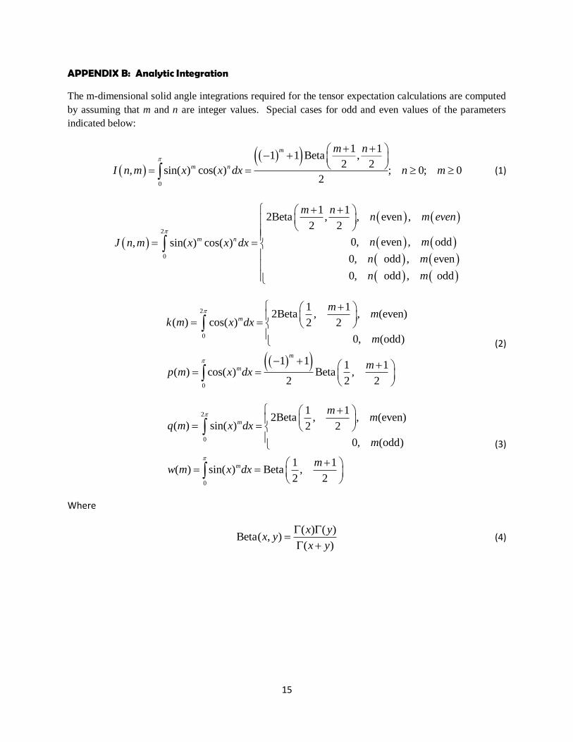
All of the angular integrals can be evaluated by table lookup, using the closed-form integrals presented

in APPENDIX B.

C. Applications

Several numerical results will be presented to demonstrate the effectiveness of the proposed symbolic

and numerical multi-dimensional Gaussian expectation operators. These examples are revisited to

demonstrate the state and the covariance uncertainty propagation for nonlinear problems5-7.

Unforced Duffing Oscillator: In this example the initial uncertainty in the state vector is propagated in time by employing first-through-fourth order of State Transition Tensor, see Figure 1. Initially, the uncertainty forms circular regimes, then it deforms based on the trajectory behavior. The state equation

is given by 3

1 2 2 1 1;x x x x x , where 1 0 1 2 0 2~ 0, 0.15 ; ~ 0, 0.15x t N x t N

Figure 1: 4th

order uncertainty propagation.

Two- Body Problem: Unperturbed Keplerian motion is governed by an inverse square gravity field. For

object motions near Earth the equation of motion is defined by3

E

r

r r , where the inertial vector of

position coordinates from the Earth center, r and μE, denote the gravitational parameters of the Earth. Bold face letters denote vectors and the corresponding unboldened letters have denote the magnitudes of these vectors, that is to say, r = |r|. The covariance propagation uncertainty is viewed in Figure 2.

Figure 2: Covaraiance propagation using State Transition Tensor Series

13

References:

1. Isserlis, L., On Certain Probable Errors and Correlation Coefficients of Multiple Frequency

Distributions with Skew Regression, Biometrika, Vol. 11, 1916, pp. 185-190. JSTOR 2331846.

2. Isserlis, L., On a formula for the product-moment coefficient of any order of a normal frequency

distribution in any number of variables, Biometrika, Vol. 12, 1918, pp. 134-139.

3. Wick, G.C., The Evaluation of the Collision Matrix, Phys. Rev. Vol. 80, 1950, pp. 268-272.

4. Michalowicz, J.V., Nichols, J.M., Bucholtz, F., and Olson, C.C., An Isserlis’ Theorem for Mixed

Gaussian Variables: Application to the Auto-Bispectral Density, J. Stat. Phys, Vol. 136, 2009, pp. 89-

102.

5. Turner, J. D., Majji, M., and Junkins, J. L., “Keynote Paper: High Accuracy trajectory and Uncertainty

Propagation Algorithm for Long-Term Asteroid Motion Prediction,” Presented to International

Conference on Computational and Experimental Engineering & Sciences, Nanjing, China, 17-21 April

2001.

6. Bani Younes, A. H., Turner, J. D., Majji, M., and Junkins, J. L., “High-Order Uncertainty propagation

Enabled by Computational Differentiation ,” Presented to 6th International Conference on

Automatic Differentiation will be held in Fort Collins, CO, July 23 - 27, 2012.

7. Majji, M., Junkins, J.L., Turner, J.D.:"A high order method for estimation of dynamic systems" J.

Astronaut. Sci. 56(3), (July–September, 2008).

14

APPENDIX A: Symbolic Macsyma Code

The successful generation of symbolic partial derivatives builds on exploiting the observations

2 3

, , , , , ,

, , , , ,; ; 0

t

k j j k j j

k j j k l

k k l k l m

R R RR R

s s s s s s

s s / 2 s ss

where only the second term survives after the evaluation of the limit condition as s=>0.

kill(all);

/*

.....Define gradient operators for multidimensional integrals

s Denotes nx1 vector

r Denotes nxn matrix (Covariance)

rs* Denotes nx1 vector where rs* = R(*,:)*S(:)

rab Denotes 1x1 scalar where rab = R(a,b)

Note:

Math model for Integrals is given by

integ( x x ...x *exp( -xt*inv(R)*x,x,-inf,inf) =

i j k

n

d exp( st*R*s ) d

--------------- = -----------integ( exp-xt*inv(R)*x + st*x )

ds ds ...ds ds ds ...ds

i j k i j k

NOTE: Partials w.r.t. S(*)

=============================================================

copyright(c) 2012 James D. Turner

*/

order:10;

var:[i,j,k,l,m,n,p,q,v,w,f,h];

par:makelist( concat( rs, part(var,ii)),ii,1,order);

save:par;

/*

.....Define partial derivative calculations */

for ii:1 thru order do (

/* Define partial derivatives w.r.t. exponential arg list */

apply( gradef, [strsd2, part(var,ii), part(par,ii) ] ),

/* Define second partial derivatives */

for jj: 1 thru order do

( apply( gradef, [ concat( rs, part(var,ii) ) , part(var,jj), concat( r, part(var,ii), part(var,jj) ) ] ) )

);

/*=============================*/

/*

.....Change of Variables to recover tensor components: s = 0 limit */

cv:[strsd2 =0];

junk:makelist( part(save,ii)=0,ii,1,order );

cv:append(cv,junk);

/*

.....Compute multidimensional gaussian integral partials by differentiation */

for ii: 1 thru order do ( if ii = 1 then pd:exp(strsd2),

pd:diff(pd,var[ii]), junk:count_ops(pd),

print(" "), print("ii,pd=",ii, junk), print(" "),

junk:ev(pd,cv),/*.....Evaluate Limit s=> 0 */

fortran(junk),

print("ii,pd=",ii, junk, count_ops(junk) )

);

a(n):=/* predict total number of terms(sum) and number of terms after limit(ff) */

block( [sum:0,ii,cc,ff],

for ii: 1 thru n do (

cc:num_combinations(2*n,2*ii), ff:(2*ii-1)!!, print("ii,cc,ff",ii,cc,ff),

sum:sum+cc*ff

), sum:sum+1 )

15

APPENDIX B: Analytic Integration

The m-dimensional solid angle integrations required for the tensor expectation calculations are computed

by assuming that m and n are integer values. Special cases for odd and even values of the parameters

indicated below:

0

1 11 1 Beta ,

2 2, sin( ) cos( ) ; 0; 0

2

m

m n

m n

I n m x x dx n m

(1)

2

0

1 12Beta , , even ,

2 2

0, even , odd, sin( ) cos( )

0, odd , even

0, odd , odd

m n

m nn m even

n mJ n m x x dx

n m

n m

2

0

0

1 12Beta , , (even)

( ) cos( ) 2 2

0, (odd)

1 1 1 1( ) cos( ) Beta ,

2 2 2

m

m

m

mm

k m x dx

m

mp m x dx

(2)

2

0

0

1 12Beta , , (even)

( ) sin( ) 2 2

0, (odd)

1 1( ) sin( ) Beta ,

2 2

m

m

mm

q m x dx

m

mw m x dx

(3)

Where

( ) ( )

Beta( , )( )

x yx y

x y

(4)

16

APPENDIX C: Guassian Integrals for the Case that the Mean is Nonzero

The m-dimensional multivariate normal distributions defined by

1 /21/2/2

, 2t

x R xm

xN R R e

(1)

where R denotes the covariance matrix. These calculations are particularly useful for sum of Gaussian

approximations for probability density functions. Integral solutions are required for

1

1

1

1

/21/2/2

/21/2/2

/21/2/2

/21/2/2

2

2

2

2

t

t

t

t

x R xm m

x R xm m

x R xm m

x R xm m

E R e dx

E R e dx

E R e dx

E R e dx

x x

xx xx

xxx xxx

xxxx xxxx

(2)

In every case one introduces the coordinate transformation

y x (3)

leading to

1

1

/21/2/2

/21/2/2

2

2

t

t

y R ym m

y R ym m

E R e dx

R e y dy

x x

(4)

because the first moment integral vanishes for gaussian variables. The second moment integral is given

by

1

1

1

/21/2/2

/21/2/2

/21/2/2

2

2

2

t

t

t

x R xm m

y R ym m

y R ym m

E xx R e dx

R e y y dy

R e yy y y dy

R

xx

(5)

where the first order moment integrals vanish and the second-order moment integral has been shown

to be the covariance matrix in Eq. (17). The third moment integral is given by

17

1

1

1

1

/21/2/2

/21/2/2

/21/2/2

/21/2/2

2

2

2

2

t

t

t

t

x R xm m

y R ym m

y R ym m

y R ym m

i j k ik j jk i ij k

yyy y y yy y yy y y

y y yy yy

E R e dx

R e y y y dy

R e dy

R e dy

E R R R

xxx xxx

x x x i j k

(6)

The fourth-order integral is given by

1

1

/21/2/2

/21/2/2

2

2

i j k l i j kl i k jl j k il i l jk j l ik k l ij i j k l

t

t

x R xm m

y R ym m

i j k l E y y y y R R R R R R

E R e dx

R e y y y y dy

E

xxxx xxxx

x x x x

(7)

where

i j k l ij kl ik jl il jkE y y y y R R R R R R (8)

as shown by Eq. (18). Higher-order integrals follow a similar pattern.