jeremy yallop - university of cambridgejdy22/papers/dissertation.pdf · to justify this approach we...
TRANSCRIPT
Abstraction for web programming
Jeremy Yallop
TH
E
U N I V E RS
IT
Y
OF
ED I N B U
RG
H
Doctor of Philosophy
Laboratory for Foundations of Computer Science
School of Informatics
University of Edinburgh
2010

Abstract
This thesis considers several instances of abstraction that arose in the design and implemen-
tation of the web programming language Links. The first concerns user interfaces, specified
using HTML forms. We wish to construct forms from existing form fragments without in-
troducing dependencies on the implementation details of those fragments. Surprisingly, many
existing web systems do not support this simple scenario. We present a library which captures
the essence of form abstraction, and extend it with more practical facilities, such as validation
of the HTML a program produces and of the input a user submits.
An important part of our library is a simple semantics, given as the composition of three
primitive “idioms”, an interface to computation introduced by McBride and Paterson. In order
to justify this approach we present a comparison of idioms with the related notions of monads
and arrows, refining the informal claims in the literature.
Our library forms part of the Links framework for stateless web interactions. We describe a
related aspect of this system, a preprocessor that derives generic instances of functions, which
we use to serialise server state between client requests. The abstraction in this case involves
the shape of datatypes: the serialisation operation is specified independently of the particular
types involved.
Our final instance of abstraction involves abstract types. Functional programming lan-
guages typically offer one of two styles of abstract type: the abstraction boundary may be
drawn using a private data constructor, or using a type signature. We show that there is a pair
of semantics-preserving translations between these two styles. In the light of this, we revisit
the decision of the Haskell designers to offer the constructor style, and define a library that
supports signature-style definitions in Haskell by translation into the constructor style.
iii
Acknowledgements
I would like to thank my supervisor, Philip Wadler, for encouraging me to come to Edinburgh,
and for his support, guidance, and inspiration throughout my time here. His comments on
earlier drafts of this thesis led to significant improvements.
I am grateful to my colleagues on the Links project, Sam Lindley and Ezra Cooper, for our
enjoyable collaboration.
Discussions with visitors to the group also improved my understanding and led me to revise
my views on more than one occasion. I particularly remember the visits of Thierry Martinez,
Shriram Krishnamurthi, and Don Syme in this regard.
Conversations with Bob Atkey led to several improvements in the ideas presented here.
My time in Edinburgh has been enriched by the wide variety of talks and seminars on offer.
In particular, the Scottish Programming Languages Seminar brought together researchers from
across Scotland, both “squigglers” and “bodgers”, and the result was invariably stimulating.
The pl-read group offered many introductions to interesting work. Thanks to the organisers
and participants.
Finally, I would like to thank Claire, Elizabeth, Amy, and Hannah, for unwavering love and
support.
My PhD studies were funded by EPSRC.
iv
Declaration
I declare that this thesis was composed by myself and that the work contained therein is my
own, except where explicitly stated otherwise below.
The paragraph describing Links in the introduction (Section 1.5) is taken from joint work
with Ezra Cooper, Sam Lindley and Philip Wadler, previously published in the proceedings
of Formal Methods for Components and Objects 2006 (Cooper, Lindley, Wadler, and Yallop,
2006).
Section 2.3 is based on joint work with Sam Lindley and Philip Wadler, previously pub-
lished in the Journal of Functional Programming (Lindley, Wadler, and Yallop, 2010). An
earlier version appeared as a technical report (Lindley, Wadler, and Yallop, 2008a).
Section 2.4 is based on joint work with Sam Lindley and Philip Wadler, to appear in the
proceedings of Mathematically Structured Functional Programming 2008 (Lindley, Wadler,
and Yallop, 2008b).
Chapter 3 is based on joint work with Ezra Cooper, Sam Lindley and Philip Wadler, pre-
viously published in the proceedings ofthe Asian Symposium on Programming Languages and
Systems 2008 (Cooper, Lindley, Wadler, and Yallop, 2008a). An earlier version appeared as a
technical report. (Cooper, Lindley, Wadler, and Yallop, 2008b).
Appendix B.2 is based on ideas from Sam Lindley’s 2008 ML Workshop paper (Lindley,
2008); the presentation given here is original. It is included for completeness, since it is closely
connected with the work described in Chapter 3.
(Jeremy Yallop)
v

Table of Contents
1 Introduction 1
1.1 Abstraction . . . . . . . . . . . . . . . . . . . . . . . . . . . . . . . . . . . . 1
1.2 Effects . . . . . . . . . . . . . . . . . . . . . . . . . . . . . . . . . . . . . . . 3
1.3 Serialising continuations . . . . . . . . . . . . . . . . . . . . . . . . . . . . . 4
1.4 Abstract types . . . . . . . . . . . . . . . . . . . . . . . . . . . . . . . . . . . 8
1.5 Links . . . . . . . . . . . . . . . . . . . . . . . . . . . . . . . . . . . . . . . 9
1.6 Contributions . . . . . . . . . . . . . . . . . . . . . . . . . . . . . . . . . . . 10
1.7 Roadmap . . . . . . . . . . . . . . . . . . . . . . . . . . . . . . . . . . . . . 11
2 Three models for the description of computation 15
2.1 Introduction . . . . . . . . . . . . . . . . . . . . . . . . . . . . . . . . . . . . 15
2.2 Arrows, idioms and monads . . . . . . . . . . . . . . . . . . . . . . . . . . . 17
2.2.1 Monads . . . . . . . . . . . . . . . . . . . . . . . . . . . . . . . . . . 17
2.2.2 Arrows . . . . . . . . . . . . . . . . . . . . . . . . . . . . . . . . . . 21
2.2.3 Idioms . . . . . . . . . . . . . . . . . . . . . . . . . . . . . . . . . . 31
2.2.4 Monoids . . . . . . . . . . . . . . . . . . . . . . . . . . . . . . . . . 37
2.2.5 Normal forms . . . . . . . . . . . . . . . . . . . . . . . . . . . . . . . 38
2.3 Two views of arrows . . . . . . . . . . . . . . . . . . . . . . . . . . . . . . . 47
2.3.1 Classic arrows . . . . . . . . . . . . . . . . . . . . . . . . . . . . . . 48
2.3.2 Arrow calculus . . . . . . . . . . . . . . . . . . . . . . . . . . . . . . 49
2.3.3 Translations . . . . . . . . . . . . . . . . . . . . . . . . . . . . . . . . 54
2.3.4 Normal forms . . . . . . . . . . . . . . . . . . . . . . . . . . . . . . . 63
2.3.5 Redundancy of the second law . . . . . . . . . . . . . . . . . . . . . . 64
2.4 Formal comparison of strength . . . . . . . . . . . . . . . . . . . . . . . . . . 67
2.4.1 Idioms and arrows . . . . . . . . . . . . . . . . . . . . . . . . . . . . 67
2.4.2 Arrows and monads . . . . . . . . . . . . . . . . . . . . . . . . . . . 75
2.4.3 Closing remarks on expressive power . . . . . . . . . . . . . . . . . . 81
vii
2.5 Future work . . . . . . . . . . . . . . . . . . . . . . . . . . . . . . . . . . . . 84
3 Abstracting controls 87
3.1 Introduction . . . . . . . . . . . . . . . . . . . . . . . . . . . . . . . . . . . . 87
3.2 Formlets by example . . . . . . . . . . . . . . . . . . . . . . . . . . . . . . . 88
3.2.1 Syntactic sugar . . . . . . . . . . . . . . . . . . . . . . . . . . . . . . 91
3.2.2 Life without formlets . . . . . . . . . . . . . . . . . . . . . . . . . . . 92
3.3 Semantics . . . . . . . . . . . . . . . . . . . . . . . . . . . . . . . . . . . . . 92
3.3.1 A concrete implementation . . . . . . . . . . . . . . . . . . . . . . . . 93
3.3.2 Idioms . . . . . . . . . . . . . . . . . . . . . . . . . . . . . . . . . . 94
3.3.3 Factoring formlets . . . . . . . . . . . . . . . . . . . . . . . . . . . . 94
3.3.4 A note on monads and arrows . . . . . . . . . . . . . . . . . . . . . . 97
3.4 Syntax . . . . . . . . . . . . . . . . . . . . . . . . . . . . . . . . . . . . . . . 98
3.4.1 Completeness . . . . . . . . . . . . . . . . . . . . . . . . . . . . . . . 101
3.5 Pragmatics . . . . . . . . . . . . . . . . . . . . . . . . . . . . . . . . . . . . . 101
3.6 Extensions . . . . . . . . . . . . . . . . . . . . . . . . . . . . . . . . . . . . . 103
3.6.1 XHTML validation . . . . . . . . . . . . . . . . . . . . . . . . . . . . 103
3.6.2 Input validation . . . . . . . . . . . . . . . . . . . . . . . . . . . . . . 105
3.6.3 Multi-holed contexts . . . . . . . . . . . . . . . . . . . . . . . . . . . 109
3.6.4 Other extensions . . . . . . . . . . . . . . . . . . . . . . . . . . . . . 110
3.7 Implementations . . . . . . . . . . . . . . . . . . . . . . . . . . . . . . . . . 110
3.8 Related work . . . . . . . . . . . . . . . . . . . . . . . . . . . . . . . . . . . 111
3.9 Conclusions . . . . . . . . . . . . . . . . . . . . . . . . . . . . . . . . . . . . 112
4 Serialising continuations 115
4.1 Introduction . . . . . . . . . . . . . . . . . . . . . . . . . . . . . . . . . . . . 115
4.1.1 Requirements . . . . . . . . . . . . . . . . . . . . . . . . . . . . . . . 115
4.1.2 Existing approaches . . . . . . . . . . . . . . . . . . . . . . . . . . . 116
4.2 Generic functions . . . . . . . . . . . . . . . . . . . . . . . . . . . . . . . . . 118
4.2.1 Example: generic equality . . . . . . . . . . . . . . . . . . . . . . . . 118
4.2.2 Modules and type classes . . . . . . . . . . . . . . . . . . . . . . . . . 122
4.2.3 Types in OCaml . . . . . . . . . . . . . . . . . . . . . . . . . . . . . 123
4.2.4 Recursive functors . . . . . . . . . . . . . . . . . . . . . . . . . . . . 124
4.2.5 Implementation of generic equality . . . . . . . . . . . . . . . . . . . 126
4.2.6 Specializing generic equality . . . . . . . . . . . . . . . . . . . . . . . 127
4.2.7 Related work . . . . . . . . . . . . . . . . . . . . . . . . . . . . . . . 131
viii
4.3 Generic serialisation . . . . . . . . . . . . . . . . . . . . . . . . . . . . . . . 132
4.3.1 The pickling algorithm . . . . . . . . . . . . . . . . . . . . . . . . . . 133
4.3.2 The unpickling algorithm . . . . . . . . . . . . . . . . . . . . . . . . . 137
4.3.3 Dynamic typing . . . . . . . . . . . . . . . . . . . . . . . . . . . . . . 141
4.3.4 Sharing . . . . . . . . . . . . . . . . . . . . . . . . . . . . . . . . . . 144
4.3.5 Specialisation example: alpha-equivalence . . . . . . . . . . . . . . . 146
4.3.6 Compactness of serialised data . . . . . . . . . . . . . . . . . . . . . . 149
4.3.7 Safety . . . . . . . . . . . . . . . . . . . . . . . . . . . . . . . . . . . 150
4.3.8 Related work . . . . . . . . . . . . . . . . . . . . . . . . . . . . . . . 151
4.4 Conclusions and future work . . . . . . . . . . . . . . . . . . . . . . . . . . . 151
5 Signed and sealed 155
5.1 Introduction . . . . . . . . . . . . . . . . . . . . . . . . . . . . . . . . . . . . 155
5.2 PolyPCF with tags . . . . . . . . . . . . . . . . . . . . . . . . . . . . . . . . 159
5.2.1 Example . . . . . . . . . . . . . . . . . . . . . . . . . . . . . . . . . 159
5.2.2 Syntax . . . . . . . . . . . . . . . . . . . . . . . . . . . . . . . . . . 161
5.2.3 Typing . . . . . . . . . . . . . . . . . . . . . . . . . . . . . . . . . . 161
5.2.4 Evaluation . . . . . . . . . . . . . . . . . . . . . . . . . . . . . . . . 161
5.2.5 Equivalence . . . . . . . . . . . . . . . . . . . . . . . . . . . . . . . . 161
5.2.6 Relations . . . . . . . . . . . . . . . . . . . . . . . . . . . . . . . . . 165
5.2.7 Frame stacks . . . . . . . . . . . . . . . . . . . . . . . . . . . . . . . 165
5.2.8 Term and stack relations . . . . . . . . . . . . . . . . . . . . . . . . . 168
5.2.9 Action of type constructors on term relations . . . . . . . . . . . . . . 169
5.2.10 Fundamental Property . . . . . . . . . . . . . . . . . . . . . . . . . . 171
5.3 Tagging and untagging . . . . . . . . . . . . . . . . . . . . . . . . . . . . . . 173
5.3.1 Example . . . . . . . . . . . . . . . . . . . . . . . . . . . . . . . . . 173
5.3.2 Definition . . . . . . . . . . . . . . . . . . . . . . . . . . . . . . . . . 174
5.4 Signing and sealing . . . . . . . . . . . . . . . . . . . . . . . . . . . . . . . . 175
5.4.1 Syntax . . . . . . . . . . . . . . . . . . . . . . . . . . . . . . . . . . 175
5.4.2 Typing . . . . . . . . . . . . . . . . . . . . . . . . . . . . . . . . . . 176
5.4.3 Evaluation . . . . . . . . . . . . . . . . . . . . . . . . . . . . . . . . 177
5.4.4 Desugaring . . . . . . . . . . . . . . . . . . . . . . . . . . . . . . . . 177
5.4.5 Equivalence . . . . . . . . . . . . . . . . . . . . . . . . . . . . . . . . 178
5.5 Signed types in Haskell . . . . . . . . . . . . . . . . . . . . . . . . . . . . . . 180
5.5.1 Introduction . . . . . . . . . . . . . . . . . . . . . . . . . . . . . . . . 180
5.5.2 Example: complex numbers . . . . . . . . . . . . . . . . . . . . . . . 182
ix
5.5.3 Example: a sudoku solver . . . . . . . . . . . . . . . . . . . . . . . . 184
5.5.4 The translation . . . . . . . . . . . . . . . . . . . . . . . . . . . . . . 186
5.6 Related work . . . . . . . . . . . . . . . . . . . . . . . . . . . . . . . . . . . 193
5.7 Future work . . . . . . . . . . . . . . . . . . . . . . . . . . . . . . . . . . . . 194
6 Conclusion 197
6.1 Contributions . . . . . . . . . . . . . . . . . . . . . . . . . . . . . . . . . . . 197
6.2 The status of Links . . . . . . . . . . . . . . . . . . . . . . . . . . . . . . . . 198
A Arrow proofs 201
A.1 Arrow normalisation . . . . . . . . . . . . . . . . . . . . . . . . . . . . . . . 202
A.2 Equational correspondence between A and C . . . . . . . . . . . . . . . . . . 205
A.2.1 Proofs of Lemmas 8 and 10 . . . . . . . . . . . . . . . . . . . . . . . 205
A.2.2 The laws of A follow from the laws of C . . . . . . . . . . . . . . . . . 209
A.2.3 The laws of C follow from the laws of A . . . . . . . . . . . . . . . . . 212
A.2.4 Translating A to C and back . . . . . . . . . . . . . . . . . . . . . . . 216
A.2.5 Translating C to A and back . . . . . . . . . . . . . . . . . . . . . . . 218
A.3 Equational correspondence between S and CS . . . . . . . . . . . . . . . . . . 220
A.3.1 Extensions of Lemmas 8 and 10 . . . . . . . . . . . . . . . . . . . . . 220
A.3.2 The laws of S follow from the laws of CS . . . . . . . . . . . . . . . . 220
A.3.3 The laws of CS follow from the laws of S . . . . . . . . . . . . . . . . 225
A.3.4 Translating S to CS and back . . . . . . . . . . . . . . . . . . . . . . . 226
A.3.5 Translating CS to S and back . . . . . . . . . . . . . . . . . . . . . . . 226
A.4 Equational equivalence between I and S . . . . . . . . . . . . . . . . . . . . . 227
A.4.1 Proofs of Lemmas 13 and 14 . . . . . . . . . . . . . . . . . . . . . . . 227
A.4.2 The laws of I follow from the laws of S . . . . . . . . . . . . . . . . . 231
A.4.3 The laws of S follow from the laws of I . . . . . . . . . . . . . . . . . 233
A.4.4 Translating I to S and back . . . . . . . . . . . . . . . . . . . . . . . . 238
A.4.5 Translating S to I and back . . . . . . . . . . . . . . . . . . . . . . . . 240
A.5 Equational embedding of S into A . . . . . . . . . . . . . . . . . . . . . . . . 245
A.5.1 Proofs of Lemmas 16 and 18 . . . . . . . . . . . . . . . . . . . . . . . 245
A.5.2 The laws of S follow from the laws of A . . . . . . . . . . . . . . . . . 250
A.5.3 The laws of A follow from the laws of S . . . . . . . . . . . . . . . . . 254
A.5.4 Translating S to A and back . . . . . . . . . . . . . . . . . . . . . . . 256
A.6 Equational correspondence between H and Capp . . . . . . . . . . . . . . . . . 258
A.6.1 Extensions of Lemmas 8 and 10 . . . . . . . . . . . . . . . . . . . . . 258
x
A.6.2 The laws of H follow from the laws of Capp . . . . . . . . . . . . . . . 259
A.6.3 The laws of Capp follow from the laws of H . . . . . . . . . . . . . . . 260
A.6.4 Translating H to Capp and back . . . . . . . . . . . . . . . . . . . . . . 262
A.6.5 Translating Capp to H and back . . . . . . . . . . . . . . . . . . . . . . 263
A.7 Equational equivalence between M and H . . . . . . . . . . . . . . . . . . . . 264
A.7.1 The laws of M follow from the laws of H . . . . . . . . . . . . . . . . 264
A.7.2 The laws of H follow from the laws of M . . . . . . . . . . . . . . . . 265
A.7.3 Translating M to H and back . . . . . . . . . . . . . . . . . . . . . . 266
A.7.4 Translating H to M and back . . . . . . . . . . . . . . . . . . . . . . 268
A.8 Redundancy of ( H2) . . . . . . . . . . . . . . . . . . . . . . . . . . . . . . 271
B Formlets extras 273
B.1 The page construct . . . . . . . . . . . . . . . . . . . . . . . . . . . . . . . . 273
B.1.1 The page interface . . . . . . . . . . . . . . . . . . . . . . . . . . . . 274
B.1.2 The page syntax . . . . . . . . . . . . . . . . . . . . . . . . . . . . . 277
B.2 Multi-holed contexts . . . . . . . . . . . . . . . . . . . . . . . . . . . . . . . 279
Bibliography 287
xi

List of Figures
1.1 Constructing and processing a form . . . . . . . . . . . . . . . . . . . . . . . 5
1.2 A program in “web style” . . . . . . . . . . . . . . . . . . . . . . . . . . . . . 6
1.3 A “direct style” version of Figure 1.2 . . . . . . . . . . . . . . . . . . . . . . . 7
1.4 Idioms, arrows and monads . . . . . . . . . . . . . . . . . . . . . . . . . . . . 11
2.1 Relating idioms, arrows and monads. . . . . . . . . . . . . . . . . . . . . . . . 16
2.2 Canonical form for arrow computations. . . . . . . . . . . . . . . . . . . . . . 40
2.3 Canonical form for idiom computations. . . . . . . . . . . . . . . . . . . . . . 45
2.4 Lambda calculus, λ→×1. . . . . . . . . . . . . . . . . . . . . . . . . . . . . . 50
2.5 Classic arrows, C (extends λ→×1, Figure 2.4). . . . . . . . . . . . . . . . . . . 51
2.6 The arrow calculus, A (extends λ→×1, Figure 2.4). . . . . . . . . . . . . . . . 52
2.7 Translating A into C. . . . . . . . . . . . . . . . . . . . . . . . . . . . . . . . 58
2.8 Translating C into A. . . . . . . . . . . . . . . . . . . . . . . . . . . . . . . . 59
2.9 Proof of (right) in C. . . . . . . . . . . . . . . . . . . . . . . . . . . . . . . . 62
2.10 Proof of ( 2) in A. . . . . . . . . . . . . . . . . . . . . . . . . . . . . . . . . 63
2.11 Translating L •M to C and back. . . . . . . . . . . . . . . . . . . . . . . . . . 64
2.12 Translating >>> to A and back. . . . . . . . . . . . . . . . . . . . . . . . . . . 65
2.13 The ( 2) law is redundant. . . . . . . . . . . . . . . . . . . . . . . . . . . . . 66
2.14 Idioms, I (extends λ→×1, Figure 2.4). . . . . . . . . . . . . . . . . . . . . . . 67
2.15 Classic arrows with delay, CS (extends C, Figure 2.5). . . . . . . . . . . . . . . 68
2.16 Static arrows, S (extends A, Figure 2.6). . . . . . . . . . . . . . . . . . . . . . 69
2.17 Translating between S and CS. . . . . . . . . . . . . . . . . . . . . . . . . . . 69
2.18 Translating between I and S. . . . . . . . . . . . . . . . . . . . . . . . . . . . 71
2.19 Embedding S into A. . . . . . . . . . . . . . . . . . . . . . . . . . . . . . . . 74
2.20 Relating idioms to arrows. . . . . . . . . . . . . . . . . . . . . . . . . . . . . 76
2.21 Monads, M (extends λ→×1, Figure 2.4). . . . . . . . . . . . . . . . . . . . . . 76
2.22 Classic arrows with apply, Capp (extends C, Figure 2.5). . . . . . . . . . . . . . 77
xiii
2.23 Higher-order arrows, H (extends A, Figure 2.6). . . . . . . . . . . . . . . . . . 77
2.24 Translating between H and Capp. . . . . . . . . . . . . . . . . . . . . . . . . . 78
2.25 Translating between M and H. . . . . . . . . . . . . . . . . . . . . . . . . . . 79
2.26 Relating arrows to monads. . . . . . . . . . . . . . . . . . . . . . . . . . . . . 81
3.1 Date example . . . . . . . . . . . . . . . . . . . . . . . . . . . . . . . . . . . 89
3.2 Date example (desugared and simplified) . . . . . . . . . . . . . . . . . . . . . 89
3.3 The xml abstract type. . . . . . . . . . . . . . . . . . . . . . . . . . . . . . . 91
3.4 The idiom interface . . . . . . . . . . . . . . . . . . . . . . . . . . . . . . . . 93
3.5 The formlet interface . . . . . . . . . . . . . . . . . . . . . . . . . . . . . . . 93
3.6 The formlet idiom . . . . . . . . . . . . . . . . . . . . . . . . . . . . . . . . . 94
3.7 The name generation idiom . . . . . . . . . . . . . . . . . . . . . . . . . . . 95
3.8 The environment idiom . . . . . . . . . . . . . . . . . . . . . . . . . . . . . . 95
3.9 The XML accumulation idiom . . . . . . . . . . . . . . . . . . . . . . . . . . 96
3.10 Idiom composition . . . . . . . . . . . . . . . . . . . . . . . . . . . . . . . . 96
3.11 The formlet idiom (factored) . . . . . . . . . . . . . . . . . . . . . . . . . . . 97
3.12 Quasiquote syntax. . . . . . . . . . . . . . . . . . . . . . . . . . . . . . . . . 99
3.13 Desugaring XML and formlets. . . . . . . . . . . . . . . . . . . . . . . . . . 100
3.14 The indexed idiom interface . . . . . . . . . . . . . . . . . . . . . . . . . . . 103
3.15 MiniXHTML fragment . . . . . . . . . . . . . . . . . . . . . . . . . . . . . . 104
3.16 The XML-indexed formlet interface . . . . . . . . . . . . . . . . . . . . . . . 105
3.17 The input-validating formlet interface . . . . . . . . . . . . . . . . . . . . . . 105
3.18 The input-validating formlet checked_int. . . . . . . . . . . . . . . . . . . . 106
3.19 The input-checking formlet positive_int. . . . . . . . . . . . . . . . . . . . 106
3.20 The failure idiom . . . . . . . . . . . . . . . . . . . . . . . . . . . . . . . . . 107
3.21 The input-validating formlet implementation . . . . . . . . . . . . . . . . . . . 108
3.22 Date example, desugared using multi-holed contexts . . . . . . . . . . . . . . 109
3.23 The parameterised idiom interface . . . . . . . . . . . . . . . . . . . . . . . . 110
4.1 Deriving equality functions for types . . . . . . . . . . . . . . . . . . . . . . . 119
4.2 Using generic equality . . . . . . . . . . . . . . . . . . . . . . . . . . . . . . 119
4.3 Output of deriving for Figure 4.1 . . . . . . . . . . . . . . . . . . . . . . . . . 120
4.4 Output of deriving for Figure 4.2 . . . . . . . . . . . . . . . . . . . . . . . . . 120
4.5 Signature of the Eq class . . . . . . . . . . . . . . . . . . . . . . . . . . . . . 121
4.6 Deriving signatures for equality . . . . . . . . . . . . . . . . . . . . . . . . . 121
4.7 Output of deriving for Figure 4.6 . . . . . . . . . . . . . . . . . . . . . . . . . 121
xiv
4.8 Correspondence between type classes and modules . . . . . . . . . . . . . . . 122
4.9 OCaml type language . . . . . . . . . . . . . . . . . . . . . . . . . . . . . . . 124
4.10 OCaml type language, normalised . . . . . . . . . . . . . . . . . . . . . . . . 125
4.11 Generation of the eq function (1) . . . . . . . . . . . . . . . . . . . . . . . . . 128
4.12 Generation of the eq function (2) . . . . . . . . . . . . . . . . . . . . . . . . . 129
4.13 Integer sets using integer lists . . . . . . . . . . . . . . . . . . . . . . . . . . . 130
4.14 Signature of the Pickle class . . . . . . . . . . . . . . . . . . . . . . . . . . 133
4.15 Generation of the pickle function . . . . . . . . . . . . . . . . . . . . . . . . 136
4.16 Generation of the unpickle function . . . . . . . . . . . . . . . . . . . . . . 139
4.17 Signature of the Typeable class . . . . . . . . . . . . . . . . . . . . . . . . . 141
4.18 The typerep type . . . . . . . . . . . . . . . . . . . . . . . . . . . . . . . . 141
4.19 Signature of the Hash class . . . . . . . . . . . . . . . . . . . . . . . . . . . . 145
4.20 Implementation of hash . . . . . . . . . . . . . . . . . . . . . . . . . . . . . 145
4.21 Generation of the Hash.merge function . . . . . . . . . . . . . . . . . . . . . 146
4.22 Using α-equivalence as equality to increase sharing . . . . . . . . . . . . . . . 148
4.23 Sharing lambda terms . . . . . . . . . . . . . . . . . . . . . . . . . . . . . . . 149
4.24 Comparative size (bytes) of the output of Pickle and Marshal serialisers . . . . 150
5.1 Abstraction schemes . . . . . . . . . . . . . . . . . . . . . . . . . . . . . . . 157
5.2 An abstract type of complex numbers in extended PolyPCF . . . . . . . . . . . 160
5.3 Syntax of the PolyPCF language extended with tags [Pitts’ Figure 1] . . . . . . 162
5.4 Typing assignment relation for PolyPCF with tags [Pitts’ Figure 2] . . . . . . . 163
5.5 PolyPCF evaluation relation [Pitts’ Figure 3] . . . . . . . . . . . . . . . . . . . 164
5.6 Compatibility properties [Pitts’ Figure 4] . . . . . . . . . . . . . . . . . . . . . 166
5.7 Substitutivity properties [Pitts’ Figure 5] . . . . . . . . . . . . . . . . . . . . . 166
5.8 Typing frame stacks [Pitts’ Figure 6] . . . . . . . . . . . . . . . . . . . . . . . 168
5.9 Structural termination relation [Pitts’ Figure 7] . . . . . . . . . . . . . . . . . 169
5.10 Definition of the logical relation ∆ [Pitts’ Figure 8] . . . . . . . . . . . . . . . 171
5.11 (Subset of) Haskell syntax . . . . . . . . . . . . . . . . . . . . . . . . . . . . 180
A.1 Index to proofs . . . . . . . . . . . . . . . . . . . . . . . . . . . . . . . . . . 201
B.1 The monoid interface . . . . . . . . . . . . . . . . . . . . . . . . . . . . . . . 274
B.2 The page interface . . . . . . . . . . . . . . . . . . . . . . . . . . . . . . . . . 274
B.3 Auxiliary types used to implement pages . . . . . . . . . . . . . . . . . . . . . 275
B.4 The page implementation . . . . . . . . . . . . . . . . . . . . . . . . . . . . . 276
xv
B.5 Page syntax. . . . . . . . . . . . . . . . . . . . . . . . . . . . . . . . . . . . 277
B.6 Desugaring pages. . . . . . . . . . . . . . . . . . . . . . . . . . . . . . . . . 278
B.7 The untyped multi-holed context abstract type . . . . . . . . . . . . . . . . . . 279
B.8 An implementation of Figure B.7 . . . . . . . . . . . . . . . . . . . . . . . . . 280
B.9 Type-level peano numbers . . . . . . . . . . . . . . . . . . . . . . . . . . . . 281
B.10 The typed multi-holed context interface . . . . . . . . . . . . . . . . . . . . . 281
B.11 The typed multi-holed context implementation . . . . . . . . . . . . . . . . . . 282
B.12 The multi-holed XML accumulation parameterised idiom . . . . . . . . . . . . 283
B.13 The multi-holed formlet interface . . . . . . . . . . . . . . . . . . . . . . . . . 283
B.14 Composition of an idiom and a parameterised idiom . . . . . . . . . . . . . . . 284
B.15 The multi-holed formlet implementation . . . . . . . . . . . . . . . . . . . . . 284
B.16 Formlet desugaring based on multi-holed contexts . . . . . . . . . . . . . . . . 285
xvi
Chapter 1
Introduction
1.1 Abstraction
Abstraction makes programs more flexible by imposing a rigid separation between use and
definition. At the value level, lambda abstraction separates out the values used in an expression.
At the type level, an abstract type definition separates the parts of a program that make use of
a type from the definition of the representation of that type.
In each case we bind a concept (such as “a date”, or “the type of dates”) to a name (such
as d, or Date), and then use that name, rather than the definition of the concept, within the
remainder of the program. Abstraction isolates each definition within a single portion of the
program; if we later change our mind about the details of the definition then the changes to our
program will be confined to that portion.
Form abstraction
Can we apply these principles of abstraction to web programming? Let us briefly review the
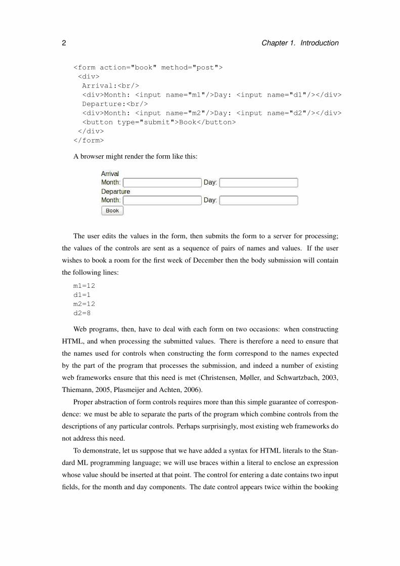
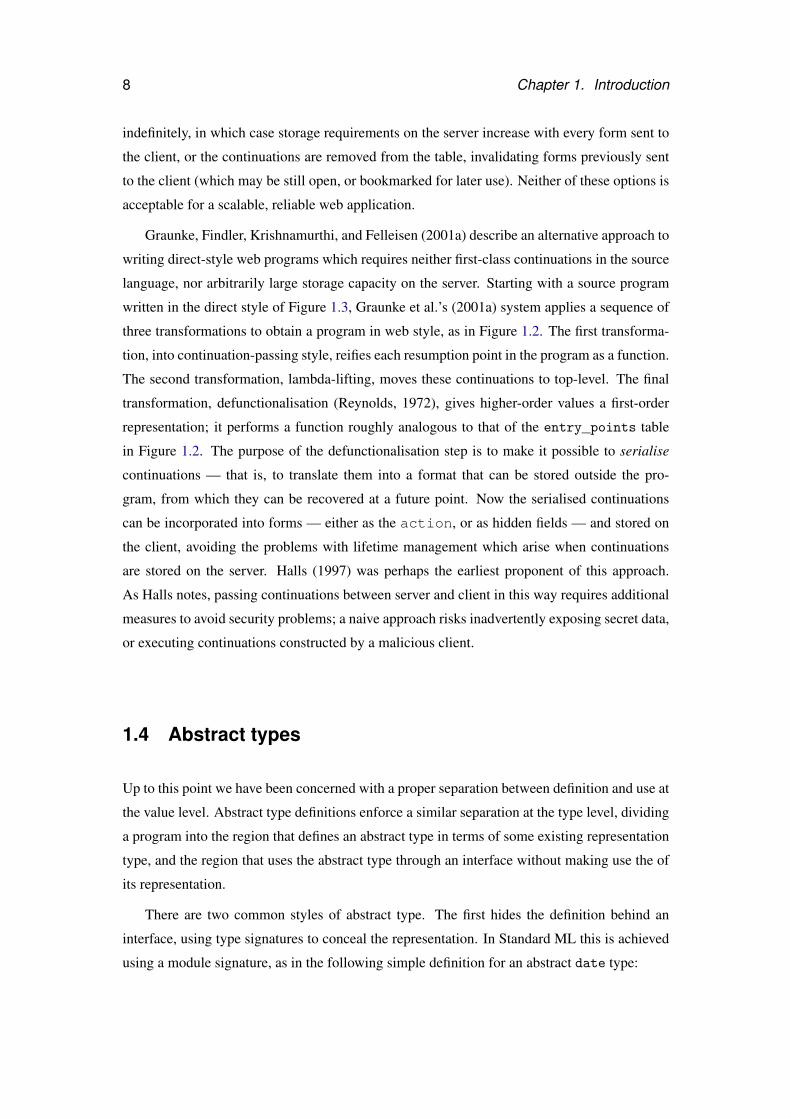
interface for interaction on the web. A web page specified using the HTML markup language
may contain one or more forms. Each of these forms contains various controls (buttons, menus,
text input boxes, and so on), each of which has a name that is unique within the form. For
example, here is the HTML for a form that allows the user to enter arrival and departure dates
for booking a hotel:
1
2 Chapter 1. Introduction
<form action="book" method="post"><div>Arrival:<br/><div>Month: <input name="m1"/>Day: <input name="d1"/></div>Departure:<br/><div>Month: <input name="m2"/>Day: <input name="d2"/></div><button type="submit">Book</button></div>
</form>
A browser might render the form like this:
The user edits the values in the form, then submits the form to a server for processing;
the values of the controls are sent as a sequence of pairs of names and values. If the user
wishes to book a room for the first week of December then the body submission will contain
the following lines:
m1=12d1=1m2=12d2=8
Web programs, then, have to deal with each form on two occasions: when constructing
HTML, and when processing the submitted values. There is therefore a need to ensure that
the names used for controls when constructing the form correspond to the names expected
by the part of the program that processes the submission, and indeed a number of existing
web frameworks ensure that this need is met (Christensen, Møller, and Schwartzbach, 2003,
Thiemann, 2005, Plasmeijer and Achten, 2006).
Proper abstraction of form controls requires more than this simple guarantee of correspon-
dence: we must be able to separate the parts of the program which combine controls from the
descriptions of any particular controls. Perhaps surprisingly, most existing web frameworks do
not address this need.
To demonstrate, let us suppose that we have added a syntax for HTML literals to the Stan-
dard ML programming language; we will use braces within a literal to enclose an expression
whose value should be inserted at that point. The control for entering a date contains two input
fields, for the month and day components. The date control appears twice within the booking
1.2. Effects 3
form, but with distinct names for the fields in each case. We therefore define the date control
as a function which accepts field names as arguments and returns the HTML for the control.
fun date m d =<div>
Month: <input name="{m}"/> Day:<input name="{d}"/></div>
The date control can now be used multiple times within a larger control, so long as fresh
names are supplied as arguments each time. Of course, to make the larger control reusable in
the same way we must abstract these names again. Here is part of our booking control again,
built from two instances of the date control above:
fun date_range m1 d1 m2 d2 =<div>
Arrival:<br/> {date m1 d1}Departure:<br/> {date m2 d2}<button type="submit">Book</button>
</div>
This passing around of names is rather inconvenient, not least since it is the responsibility
of the caller to avoid name clashes. However, there is a more serious problem. Suppose that
we wish to change the definition of the booking control to contain a single field for entering a
free form date.
fun date d =<div>
<input name="{d}"/></div>
We now have to change the definition not only of date, but of date_range, and every other
place in the program where the date control is used. We call this breakdown in modularity the
form abstraction problem: the “clients” of a definition are written in a way that depends upon
the internal details of that definition. The abstraction leaks.
1.2 Effects
Our solution to the form abstraction problem involves a domain-specific language for describ-
ing forms; we embed this language into a “host” functional programming language. The func-
tional programming style discourages the use of side effects, but form processing naturally
involves certain effects: for example, we must generate unique names for fields during form
generation and look up values in the environment during processing of a submission. As we
4 Chapter 1. Introduction
have seen, it is possible to avoid these effects by threading state (such as the names needed by
a component) throughout the program, but this can lead to an awkward programming style and
a loss of abstraction.
There are several approaches to resolving the tension between the convenience of effects
and the benefits of purity. An approach that has proven fruitful in Haskell (Peyton Jones and
Hughes, 1999) is to shift the focus from executing effectful computations to constructing com-
putations that can be executed later. Using this approach, computations are reified as regular
values, and sequencing of computations is simply composition of values. It is this approach
that we shall use in developing a solution to the form abstraction problem.
Monads (Moggi, 1989, Wadler, 1990) are the most popular and most powerful example
of the computations-as-values approach. The monad interface is used for the standard I/O
interface in Haskell, besides many other “notions of computation” ranging from parsers (Hutton
and Meijer, 1998) to database queries (Leijen and Meijer, 1999). The interface provides great
flexibility in constructing and sequencing computations; in particular, it enables higher-order
programming, in which computations can be constructed and executed “on-the-fly”. However,
the power comes with a price: every implementation of the monad interface must offer the
same flexibility. When the underlying notion of computation does not support the required
degree of flexibility the monad interface cannot be used.
Two alternatives to the monad interface have been suggested. Hughes (2000) introduced
arrows as a kind of first-order variant of monads. McBride and Paterson (2008) introduced
idioms (also known as applicative functors) as an interface for writing effectful computations
in an applicative style; as with arrows, the idiomatic interface is less powerful than the monadic.
In order to choose the most suitable interface for defining composable form fragments we will
make a careful investigation and comparison of idioms, monads and arrows.
1.3 Serialising continuations
Let us return to the HTML form example of Section 1.1:
<form action="book" method="post">...
</form>
The action attribute of the form element is a URL indicating the program that will
process the form submission. In our example the URL is relative, and specifies a program
called book.
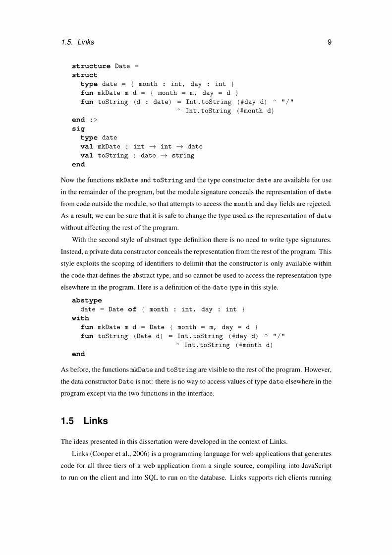
Indicating the program that will process the form submission in this way leads to a dis-
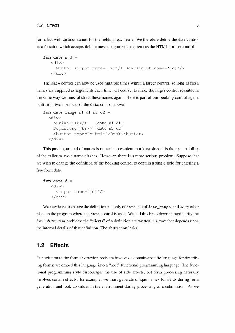
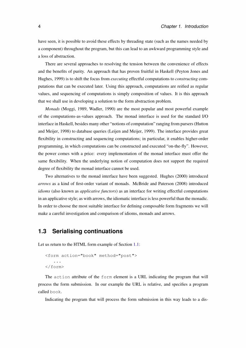
1.3. Serialising continuations 5
GET booking.html
<form action="book"> <div> ...
POST bookm1=12d1=1...
Client Server
Figure 1.1: Constructing and processing a form
tinctive structure for web programs that is similar to the continuation-passing style familiar
to functional programmers. Programs written in continuation-passing style pass an extra pa-
rameter, the continuation, to each function. When the function’s work is finished, rather than
returning a result to the calling context (as a program written in the regular, direct style does),
it calls this continuation, passing the result as an argument. Similarly, a web program con-
structs a form, passing the name of a “continuation” program as the action attribute, then
relinquishes control to the user. The user edits the fields, then “calls” the continuation program
by submitting the form (Figure 1.1).
A significant difference between the continuation-passing style used in functional programs
and the structure of web programs is that in the former continuations are often denoted by
nested function expressions, whereas the latter requires that every “continuation” to a form is a
program named at top level. This constraint is similar to the distinguishing feature of a second
class of programs, those in lambda-lifted form (Johnsson, 1985). The lambda-lifting transfor-
mation replaces each nested function expression with a top-level function, and each free vari-
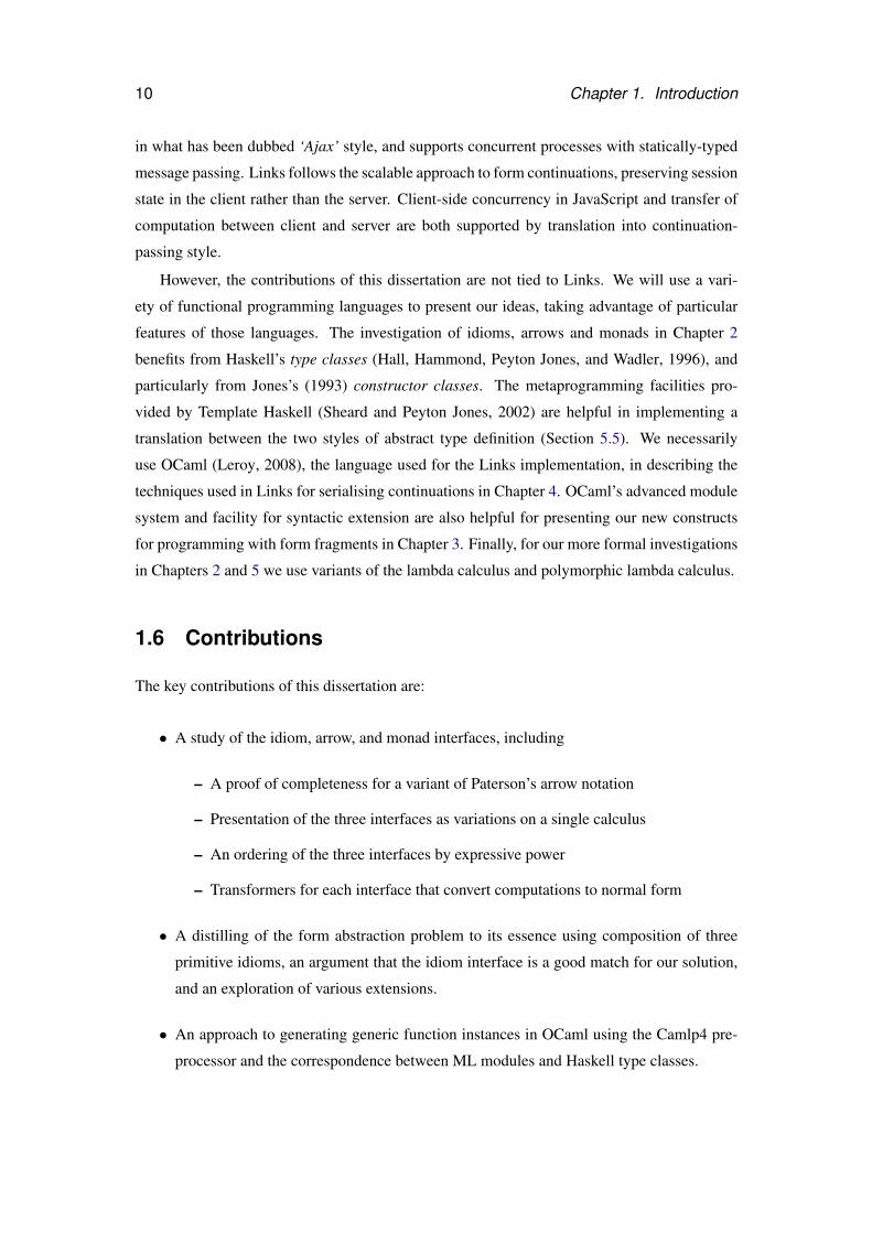
6 Chapter 1. Introduction
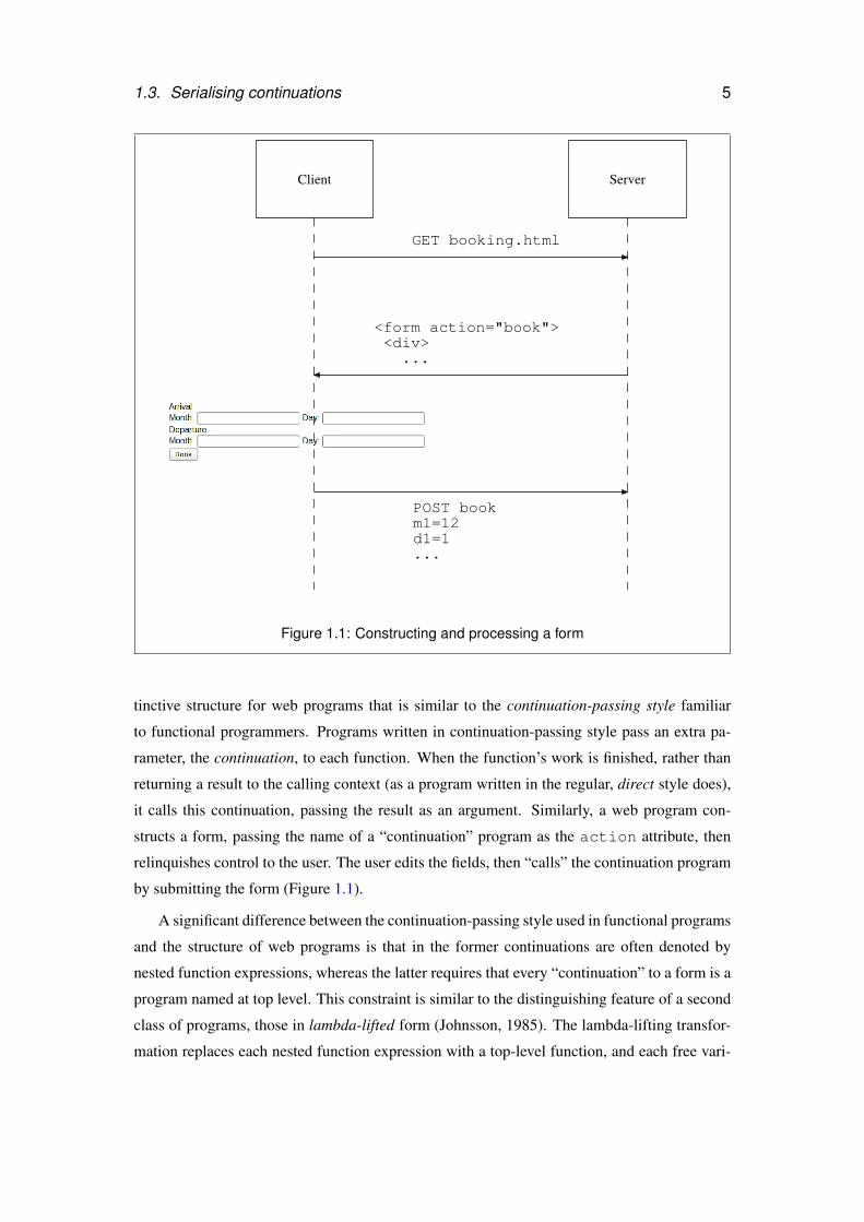
fun book env =let () = register_booking
(read_date "m1" "d1" env) (read_date "m2" "d2" env)in send_page <div>Booking confirmed!</div>
val entry_points = [ ("book", book), . . .]
send_page(<form action="book">
<div>Month: <input name="m1"/>Day: <input name="d1"/></div>
<div>Month: <input name="m2"/>Day: <input name="d2"/></div>
<button type="submit">Book</button></form>)
Figure 1.2: A program in “web style”
able in the original expression with a parameter to the function. We refer to the continuation-
passing lambda-lifted style used in web programs as “web style”.
Both the continuation-passing style and the lambda-lifted style have interesting theoreti-
cal properties, but they are inconvenient for programming; they are more suitable for use in
the internals of compilers than as source languages (Peyton Jones, 1986, Appel, 2007). Con-
sequently, Queinnec (2000) and Graunke, Krishnamurthi, Hoeven, and Felleisen (2001b) ad-
vocate using a language with first-class continuations, such as Scheme (R. Kelsey, 1998), for
writing web programs in a more direct style. A program written using Graunke et al.’s system
uses a special procedure during form construction, send/suspend, which generates a string
referring to its own continuation; this string is used as the action attribute of the form. When
the form is submitted this reference is resolved, and the continuation is invoked with the form
values entered by the user. To the programmer it appears that the form values are “returned”
from send/suspend, in contrast to the regular style of web program, where they are passed as
arguments to the entry point named in the action attribute.
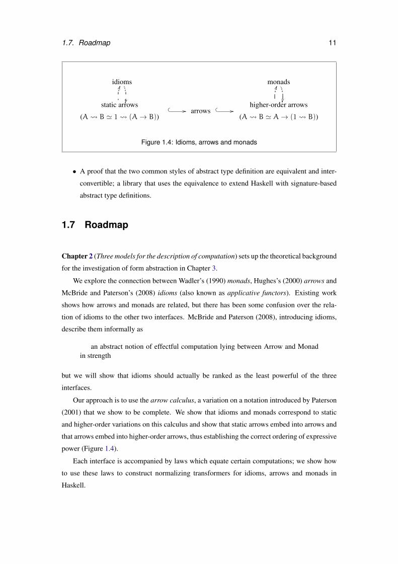
Figures 1.2 and 1.3 illustrate the two styles (using Standard ML rather than Scheme, for
continuity with the other examples in this chapter). The first program (Figure 1.2) is written
in “web style”. It creates and displays a form which names the function book as the action;
we assume a function send_page that wraps the form in suitable boilerplate HTML to form
a complete page, sends the page the client and exits the program. The book function ac-
cepts an environment containing the submitted field values, which it extracts using a function
read_date. After registering the booking (in a database, say), it sends a confirmation page
1.3. Serialising continuations 7
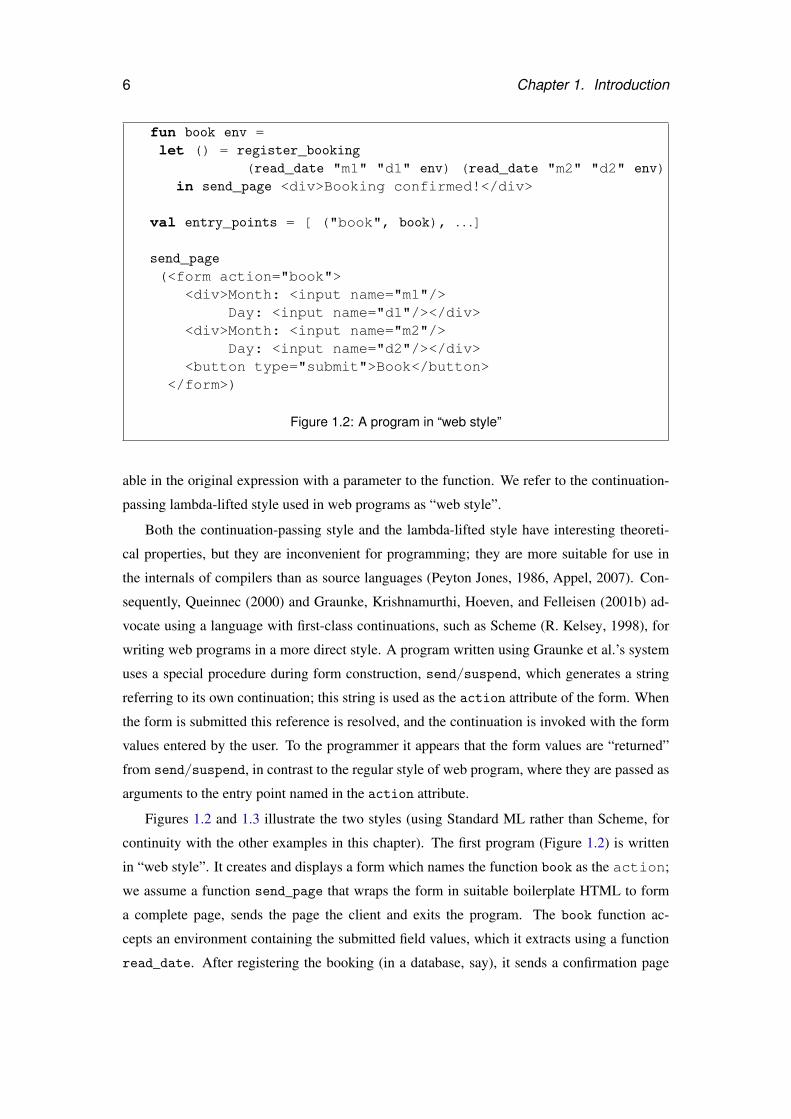
let env =(send_suspend
(fn k_url ⇒(make_page
<form action="{k_url}"><div>Month: <input name="m1"/>
Day: <input name="d1"/></div><div>Month: <input name="m2"/>
Day: <input name="d2"/></div><button type="submit">Book</button>
</form>)))inlet () = register_booking
(read_date "m1" "d1" env) (read_date "m2" "d2" env)in send_page <div>Booking confirmed!</div>
end
Figure 1.3: A “direct style” version of Figure 1.2
to the client. The entry_points variable is bound to a table which maps each name used
as the action of a form to the corresponding continuation function. (We do not show the
code which performs this resolution.) The second program (Figure 1.3) uses send_suspend
to generate a value for the action of the form and binds it to k_url. (We assume a func-
tion make_page which wraps the form in boilerplate HTML to form a complete page.) When
the form is submitted this action is resolved to the continuation of the call to send_suspend,
which is invoked with the submitted environment. This environment is bound to env, and the
program resumes execution at the point where the call to send_suspend returns; at this point
the program behaves like the book function of Figure 1.2, extracting the dates and passing the
results the register_booking.
The direct style of Figure 1.3 uses the continuation of the program that generates a response
as the entry point to the program that generates the next response. The question therefore arises
as to where to store this continuation between requests. One approach, taken by Graunke et al.
(2001b), Graham (1997), and others, is to store the continuation in a persistent table on the
server between requests, treating the string used as the action as an index into this table.
This implementation has the advantages of simplicity and efficiency: the index is small and
simple compared to the continuation, and multiple continuations involving the same data can
share structure, since they are stored in the same server. However, there are also serious short-
comings, most notably the difficulty in reclaiming the storage used by continuations. There are
two potential strategies for reclaiming storage: either the continuations in the table are stored
8 Chapter 1. Introduction
indefinitely, in which case storage requirements on the server increase with every form sent to
the client, or the continuations are removed from the table, invalidating forms previously sent
to the client (which may be still open, or bookmarked for later use). Neither of these options is
acceptable for a scalable, reliable web application.
Graunke, Findler, Krishnamurthi, and Felleisen (2001a) describe an alternative approach to
writing direct-style web programs which requires neither first-class continuations in the source
language, nor arbitrarily large storage capacity on the server. Starting with a source program
written in the direct style of Figure 1.3, Graunke et al.’s (2001a) system applies a sequence of
three transformations to obtain a program in web style, as in Figure 1.2. The first transforma-
tion, into continuation-passing style, reifies each resumption point in the program as a function.
The second transformation, lambda-lifting, moves these continuations to top-level. The final
transformation, defunctionalisation (Reynolds, 1972), gives higher-order values a first-order
representation; it performs a function roughly analogous to that of the entry_points table
in Figure 1.2. The purpose of the defunctionalisation step is to make it possible to serialise
continuations — that is, to translate them into a format that can be stored outside the pro-
gram, from which they can be recovered at a future point. Now the serialised continuations
can be incorporated into forms — either as the action, or as hidden fields — and stored on
the client, avoiding the problems with lifetime management which arise when continuations
are stored on the server. Halls (1997) was perhaps the earliest proponent of this approach.
As Halls notes, passing continuations between server and client in this way requires additional
measures to avoid security problems; a naive approach risks inadvertently exposing secret data,
or executing continuations constructed by a malicious client.
1.4 Abstract types
Up to this point we have been concerned with a proper separation between definition and use at
the value level. Abstract type definitions enforce a similar separation at the type level, dividing
a program into the region that defines an abstract type in terms of some existing representation
type, and the region that uses the abstract type through an interface without making use the of
its representation.
There are two common styles of abstract type. The first hides the definition behind an
interface, using type signatures to conceal the representation. In Standard ML this is achieved
using a module signature, as in the following simple definition for an abstract date type:
1.5. Links 9
structure Date =struct
type date = { month : int, day : int }fun mkDate m d = { month = m, day = d }fun toString (d : date) = Int.toString (#day d) ^ "/"
^ Int.toString (#month d)end :>sigtype date
val mkDate : int → int → date
val toString : date → string
end
Now the functions mkDate and toString and the type constructor date are available for use
in the remainder of the program, but the module signature conceals the representation of date
from code outside the module, so that attempts to access the month and day fields are rejected.
As a result, we can be sure that it is safe to change the type used as the representation of date
without affecting the rest of the program.
With the second style of abstract type definition there is no need to write type signatures.
Instead, a private data constructor conceals the representation from the rest of the program. This
style exploits the scoping of identifiers to delimit that the constructor is only available within
the code that defines the abstract type, and so cannot be used to access the representation type
elsewhere in the program. Here is a definition of the date type in this style.
abstypedate = Date of { month : int, day : int }
withfun mkDate m d = Date { month = m, day = d }fun toString (Date d) = Int.toString (#day d) ^ "/"
^ Int.toString (#month d)end
As before, the functions mkDate and toString are visible to the rest of the program. However,
the data constructor Date is not: there is no way to access values of type date elsewhere in the
program except via the two functions in the interface.
1.5 Links
The ideas presented in this dissertation were developed in the context of Links.
Links (Cooper et al., 2006) is a programming language for web applications that generates
code for all three tiers of a web application from a single source, compiling into JavaScript
to run on the client and into SQL to run on the database. Links supports rich clients running
10 Chapter 1. Introduction
in what has been dubbed ‘Ajax’ style, and supports concurrent processes with statically-typed
message passing. Links follows the scalable approach to form continuations, preserving session
state in the client rather than the server. Client-side concurrency in JavaScript and transfer of
computation between client and server are both supported by translation into continuation-
passing style.
However, the contributions of this dissertation are not tied to Links. We will use a vari-
ety of functional programming languages to present our ideas, taking advantage of particular
features of those languages. The investigation of idioms, arrows and monads in Chapter 2
benefits from Haskell’s type classes (Hall, Hammond, Peyton Jones, and Wadler, 1996), and
particularly from Jones’s (1993) constructor classes. The metaprogramming facilities pro-
vided by Template Haskell (Sheard and Peyton Jones, 2002) are helpful in implementing a
translation between the two styles of abstract type definition (Section 5.5). We necessarily
use OCaml (Leroy, 2008), the language used for the Links implementation, in describing the
techniques used in Links for serialising continuations in Chapter 4. OCaml’s advanced module
system and facility for syntactic extension are also helpful for presenting our new constructs
for programming with form fragments in Chapter 3. Finally, for our more formal investigations
in Chapters 2 and 5 we use variants of the lambda calculus and polymorphic lambda calculus.
1.6 Contributions
The key contributions of this dissertation are:
• A study of the idiom, arrow, and monad interfaces, including
– A proof of completeness for a variant of Paterson’s arrow notation
– Presentation of the three interfaces as variations on a single calculus
– An ordering of the three interfaces by expressive power
– Transformers for each interface that convert computations to normal form
• A distilling of the form abstraction problem to its essence using composition of three
primitive idioms, an argument that the idiom interface is a good match for our solution,
and an exploration of various extensions.
• An approach to generating generic function instances in OCaml using the Camlp4 pre-
processor and the correspondence between ML modules and Haskell type classes.
1.7. Roadmap 11
idioms
��
monads
��static arrows
(A B ' 1 (A→ B))
II
� � // arrows � � //higher-order arrows
(A B ' A→ (1 B))
II
Figure 1.4: Idioms, arrows and monads
• A proof that the two common styles of abstract type definition are equivalent and inter-
convertible; a library that uses the equivalence to extend Haskell with signature-based
abstract type definitions.
1.7 Roadmap
Chapter 2 (Three models for the description of computation) sets up the theoretical background
for the investigation of form abstraction in Chapter 3.
We explore the connection between Wadler’s (1990) monads, Hughes’s (2000) arrows and
McBride and Paterson’s (2008) idioms (also known as applicative functors). Existing work
shows how arrows and monads are related, but there has been some confusion over the rela-
tion of idioms to the other two interfaces. McBride and Paterson (2008), introducing idioms,
describe them informally as
an abstract notion of effectful computation lying between Arrow and Monadin strength
but we will show that idioms should actually be ranked as the least powerful of the three
interfaces.
Our approach is to use the arrow calculus, a variation on a notation introduced by Paterson
(2001) that we show to be complete. We show that idioms and monads correspond to static
and higher-order variations on this calculus and show that static arrows embed into arrows and
that arrows embed into higher-order arrows, thus establishing the correct ordering of expressive
power (Figure 1.4).
Each interface is accompanied by laws which equate certain computations; we show how
to use these laws to construct normalizing transformers for idioms, arrows and monads in
Haskell.
12 Chapter 1. Introduction
Chapter 3 (Abstracting controls) describes formlets, a solution to the form abstraction
problem introduced in Section 1.1. Formlets allow true abstraction over form components,
freeing the programmer from the need to worry about name collisions or type mismatch prob-
lems.
We argue that formlets are most naturally viewed as an idiom (rather than as an arrow
or monad) and give a semantics based on the composition of the three standard idioms that
capture the effects necessary for programming with forms. We also give a formal definition of
the formlet syntactic sugar and an implementation in OCaml.
Although formlets capture only the essence of form abstraction it is easy to extend the basic
definition with additional features. We describe extensions for statically checking the validity
of generated XHTML and dynamically checking that user input meets specified constraints.
We briefly discuss a more efficient desugaring translation.
Chapter 4 (Serialising continuations) describes deriving, an extension to OCaml for de-
riving generic function instances that we use to provide an essential part of the formlets imple-
mentation in Links: the serialisation of continuations.
The design of deriving is inspired by the Haskell keyword of the same name. As in Haskell,
the programmer may list the names of classes after a type declaration to request that the imple-
mentation generate instances of those classes for the declared type. OCaml does not have type
classes, but there is a well-known correspondence between modules and type classes that we
use to guide the design of deriving.
One advantage of our approach is that, in contrast to the more common approach based
on combinators, almost no effort is required on the part of the programmer in the common
case where the generated instance is adequate; however, it is also straightforward to provide
customised instances for particular types which integrate smoothly with the generated code.
Chapter 5 (Signed and Sealed) formally compares the two styles of abstract type definition,
as introduced in Section 1.4, in which the representation type is concealed from the rest of the
program using either a type signature or a private data constructor. We add constructs for
both styles to a partial polymorphic lambda calculus introduced by Pitts (2000) and give a
parametricity-based proof that the two are equivalent, together with an automatic translation
from each style into the other.
In part, our motivation comes from addressing a problem encountered by the designers
of Haskell: it was unclear how to combine the signing style of abstract type definition with
unambiguous overloading (Hudak, Hughes, Peyton Jones, and Wadler, 2007). We show that
this is possible by translating the signing style into the sealing style used by Haskell, and
1.7. Roadmap 13
describe a Template Haskell library that performs this translation. We demonstrate by examples
that the signing style can lead to more elegant Haskell programs, removing the clutter of the
constructors and destructors introduced by sealing.
Chapter 6 concludes.

Chapter 2
Three models for the description
of computation
2.1 Introduction
The Internet Robustness Principle (RFC 793) states
Be conservative in what you do; be liberal in what you accept from others.
In other words, robust systems make the weakest possible assumptions about input and
give the strongest possible guarantees about output. Programs that accept only integers are less
flexible than programs that accept all kinds of number. Contrariwise, programs that may output
any kind of number are less flexible than programs that are guaranteed to output only integers.
To follow the principle we need to know which sets of values generalise which other sets.
While there are certainly more numbers than integers, the ordering is not so obvious at higher-
order types, such as function and computation types. Can a program that manipulates arrow
computations be made more flexible by specifying that the input must be an idiom rather than
an arrow? Can a library that exposes an idiom instance be made more flexible by exposing
an arrow instance instead? In his original work on arrows, Hughes shows how each monad
gives rise to an arrow, and gives an extended arrow interface, ArrowApp, that is equivalent
to the monad interface1 (Hughes, 2000). In their later work introducing idioms, McBride and
Paterson show how to obtain an idiom from either a monad or an arrow, and how to combine an
idiom and an arrow to yield another arrow (McBride and Paterson, 2008). However, the precise
1 The title is a nod to Chomsky’s seminal work on the relative power of three classes of formal language(Chomsky, 1956), but we shall use “interface” rather than “model” to refer to the concepts “monad”, “arrow” and“idiom” in the remainder of this chapter.
15
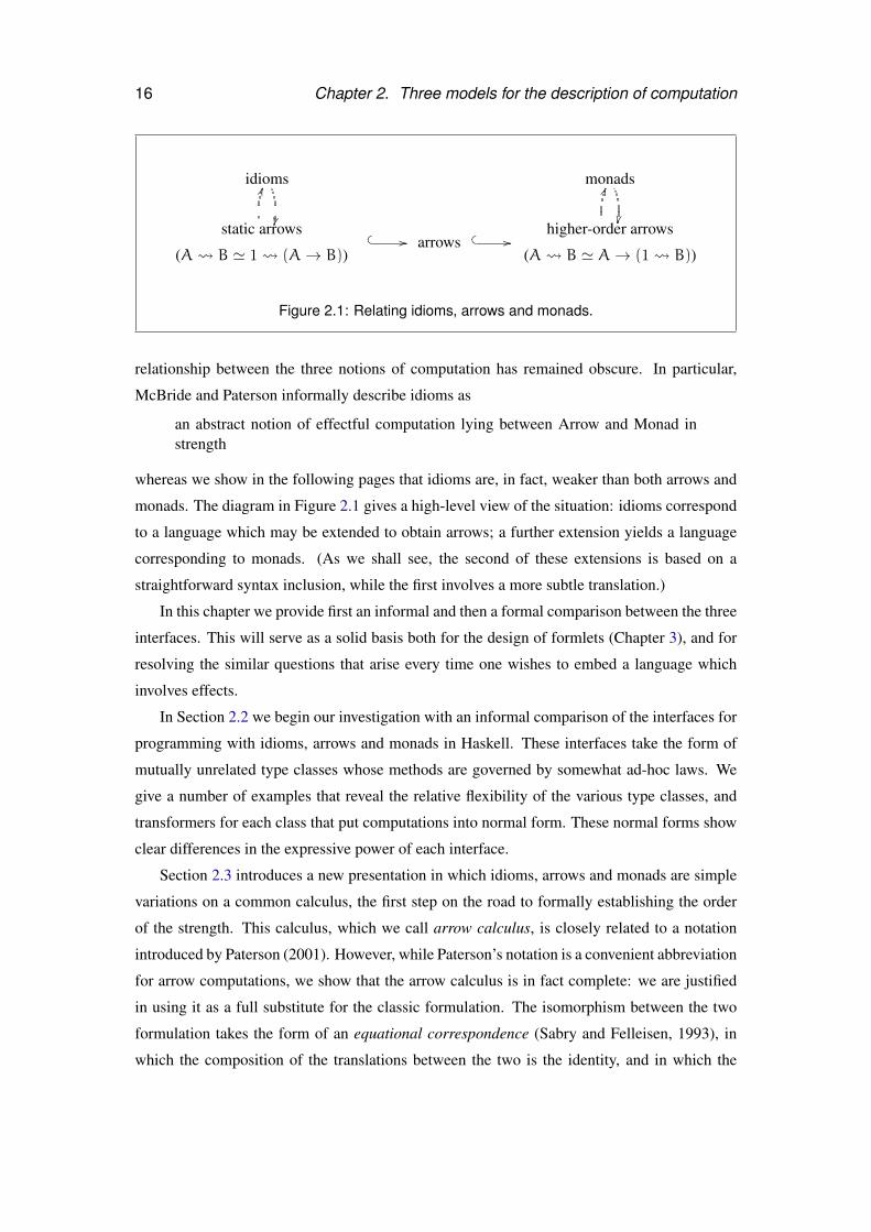
16 Chapter 2. Three models for the description of computation
idioms
��
monads
��static arrows
(A B ' 1 (A→ B))
II
� � // arrows � � //higher-order arrows
(A B ' A→ (1 B))
II
Figure 2.1: Relating idioms, arrows and monads.
relationship between the three notions of computation has remained obscure. In particular,
McBride and Paterson informally describe idioms as
an abstract notion of effectful computation lying between Arrow and Monad instrength
whereas we show in the following pages that idioms are, in fact, weaker than both arrows and
monads. The diagram in Figure 2.1 gives a high-level view of the situation: idioms correspond
to a language which may be extended to obtain arrows; a further extension yields a language
corresponding to monads. (As we shall see, the second of these extensions is based on a
straightforward syntax inclusion, while the first involves a more subtle translation.)
In this chapter we provide first an informal and then a formal comparison between the three
interfaces. This will serve as a solid basis both for the design of formlets (Chapter 3), and for
resolving the similar questions that arise every time one wishes to embed a language which
involves effects.
In Section 2.2 we begin our investigation with an informal comparison of the interfaces for
programming with idioms, arrows and monads in Haskell. These interfaces take the form of
mutually unrelated type classes whose methods are governed by somewhat ad-hoc laws. We
give a number of examples that reveal the relative flexibility of the various type classes, and
transformers for each class that put computations into normal form. These normal forms show
clear differences in the expressive power of each interface.
Section 2.3 introduces a new presentation in which idioms, arrows and monads are simple
variations on a common calculus, the first step on the road to formally establishing the order
of the strength. This calculus, which we call arrow calculus, is closely related to a notation
introduced by Paterson (2001). However, while Paterson’s notation is a convenient abbreviation
for arrow computations, we show that the arrow calculus is in fact complete: we are justified
in using it as a full substitute for the classic formulation. The isomorphism between the two
formulation takes the form of an equational correspondence (Sabry and Felleisen, 1993), in
which the composition of the translations between the two is the identity, and in which the
2.2. Arrows, idioms and monads 17
laws of each follow from the laws of the other. The proof of the correspondence reveals that
one of the laws in the standard presentation of arrows is redundant.
Section 2.4 extends the arrow calculus in two ways: first, by introducing either an addi-
tional operator or a type isomorphism to bring it into correspondence with idioms; next, by
introducing either an additional operator or a type isomorphism to bring it into correspondence
with monads. (These correspondences are weaker than the equational correspondence between
arrow calculus and classic arrows; in order to characterise them we introduce the notion of
equational equivalence.) The relationships that emerge invalidate the claim by McBride and
Paterson quoted above. The extension of arrow calculus to support higher-order (i.e. monadic)
computation also reveals that one of the laws in the standard presentation of higher-order ar-
rows is redundant.
2.2 Arrows, idioms and monads
We begin by introducing monads, arrows and idioms as they are used in Haskell. Each interface
makes computations available as first-class values within the language and provides operators
for constructing and composing computations. Haskell provides a principled form of overload-
ing, the type class (Hall et al., 1996), which is a good fit for programming with monads, arrows
and idioms.
2.2.1 Monads
Wadler (1990) introduced monads to the functional programming community, drawing on work
by Moggi (1991) on the semantics of effectful programs. Using monads, computations are
presented as first-class values, with combinators for constructing and composing computations.
Monads have proved remarkably successful as a program structuring technique: they are used,
for example, as the sole means of constructing programs which perform I/O in Haskell (Peyton
Jones and Hughes, 1999).
2.2.1.1 Monad operators
The Monad type class provides a common interface for various notions of effectful computation.
Each instance of the class consists of a unary type constructor, m, for representing computa-
tions, and two computation-forming operations, return and >>= (pronounced “bind”). The
18 Chapter 2. Three models for the description of computation
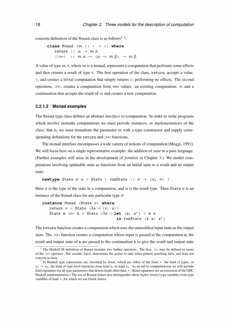
concrete definition of the Monad class is as follows2 3:
class Monad (m :: * → *) wherereturn :: α → m α
(>>=) :: m α → (α → m β) → m β
A value of typem τ, wherem is a monad, represents a computation that performs some effects
and then returns a result of type τ. The first operation of the class, return, accepts a value,
v , and creates a trivial computation that simply returns v , performing no effects. The second
operation, >>=, creates a computation from two values: an existing computation, m and a
continuation that accepts the result of m and creates a new computation.
2.2.1.2 Monad examples
The Monad type class defines an abstract interface to computation. In order to write programs
which involve monadic computations we must provide instances, or implementations of the
class; that is, we must instantiate the parameter m with a type constructor and supply corre-
sponding definitions for the return and >>= functions.
The monad interface encompasses a wide variety of notions of computation (Moggi, 1991).
We will focus here on a single representative example: the addition of state to a pure language.
(Further examples will arise in the development of formlets in Chapter 3.) We model com-
putations involving updatable state as functions from an initial state to a result and an output
state.
newtype State σ α = State { runState :: σ → (α, σ) }
Here σ is the type of the state in a computation, and α is the result type. Then State σ is an
instance of the Monad class for any particular type σ:
instance Monad (State σ) wherereturn v = State (λs→ (v, s))State m >>= k = State (λs→ let (a, s’) = m s
in runState (k a) s’)
The return function creates a computation which uses the unmodified input state as the output
state. The >>= function creates a computation whose input is passed to the computation m; the
result and output state of m are passed to the continuation k to give the result and output state2 The Haskell 98 definition of Monad includes two further operators. The first, >>, may be defined in terms
of the >>= operator. The second, fail, determines the action to take when pattern matching fails, and does notconcern us here.
3 In Haskell type expressions are classified by kinds, which are either of the form *, the kind of types, orκ1 → κ2, the kind of type-level functions from kind κ1 to kind κ2. As an aid to comprehension we will includekind signatures for all type parameters that denote kinds other than*. (Kind signatures are an extension of the GHCHaskell implementation.) The use of Roman letters also distinguishes these higher-kinded type variables from typevariables of kind *, for which we use Greek letters.
2.2. Arrows, idioms and monads 19
of the whole computation.
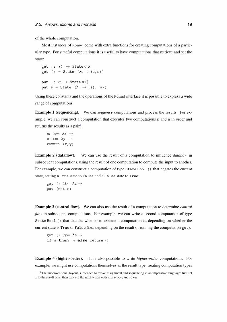
Most instances of Monad come with extra functions for creating computations of a partic-
ular type. For stateful computations it is useful to have computations that retrieve and set the
state:
get :: () → State σ σ
get () = State (λs→ (s,s))
put :: σ → State σ ()put s = State (λ_→ ((), s))
Using these constants and the operations of the Monad interface it is possible to express a wide
range of computations.
Example 1 (sequencing). We can sequence computations and process the results. For ex-
ample, we can construct a computation that executes two computations m and n in order and
returns the results as a pair4:
m >>= λx →n >>= λy →return (x,y)
Example 2 (dataflow). We can use the result of a computation to influence dataflow in
subsequent computations, using the result of one computation to compute the input to another.
For example, we can construct a computation of type State Bool () that negates the current
state, setting a True state to False and a False state to True:
get () >>= λs→put (not s)
Example 3 (control flow). We can also use the result of a computation to determine control
flow in subsequent computations. For example, we can write a second computation of type
State Bool () that decides whether to execute a computation m depending on whether the
current state is True or False (i.e., depending on the result of running the computation get):
get () >>= λs→if s then m else return ()
Example 4 (higher-order). It is also possible to write higher-order computations. For
example, we might use computations themselves as the result type, treating computation types4The unconventional layout is intended to evoke assignment and sequencing in an imperative language: first set
x to the result of m, then execute the next action with x in scope, and so on.
20 Chapter 2. Three models for the description of computation
of the form
State σ (State σ τ)
Given a computation m of this type we can write a computation of type State σ τ that executes
the result of m:
m >>= λn→n
(This computation corresponds to the multiplication of the monad.)
As we shall see in Sections 2.2.2 and 2.2.3, the other computational interfaces — Arrow
and Idiom — are only sufficiently flexible to encode some, not all, of these computations.
2.2.1.3 Monad laws
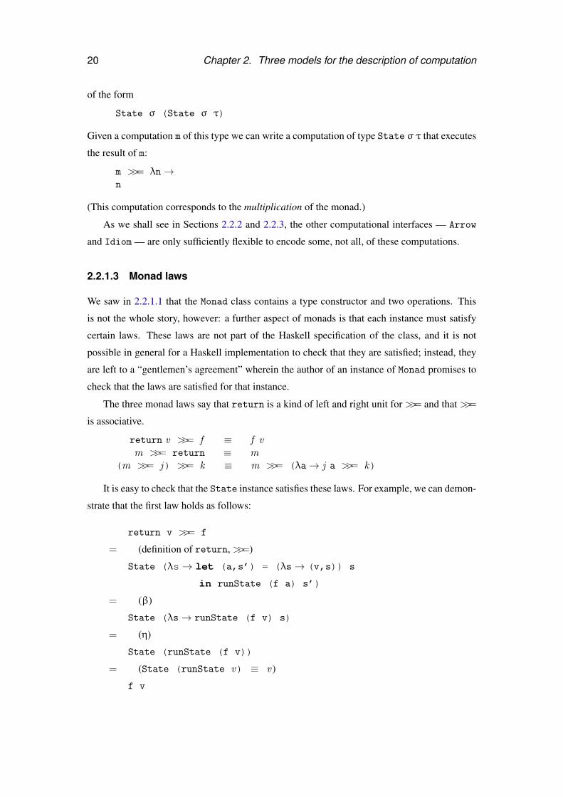
We saw in 2.2.1.1 that the Monad class contains a type constructor and two operations. This
is not the whole story, however: a further aspect of monads is that each instance must satisfy
certain laws. These laws are not part of the Haskell specification of the class, and it is not
possible in general for a Haskell implementation to check that they are satisfied; instead, they
are left to a “gentlemen’s agreement” wherein the author of an instance of Monad promises to
check that the laws are satisfied for that instance.
The three monad laws say that return is a kind of left and right unit for >>= and that >>=
is associative.
return v >>= f ≡ f vm >>= return ≡ m
(m >>= j) >>= k ≡ m >>= (λa→ j a >>= k)
It is easy to check that the State instance satisfies these laws. For example, we can demon-
strate that the first law holds as follows:
return v >>= f
= (definition of return, >>=)
State (λs→ let (a,s’) = (λs→ (v,s)) s
in runState (f a) s’)
= (β)
State (λs→ runState (f v) s)
= (η)
State (runState (f v))
= (State (runState v) ≡ v )
f v
2.2. Arrows, idioms and monads 21
It is similarly straightforward to demonstrate that the other monad laws hold for State.
2.2.2 Arrows
The examples in Section 2.2.1.2 illustrate the flexibility offered by the Monad interface. This
flexibility is a boon when writing programs which use the Monad interface, but can become a
burden when writing instances of the class.
Hughes (2000) gives a striking example of this phenomenon. Parser combinators embed
parsers in functional languages as regular values (Wadler, 1985), commonly casting them as
monads (Hutton and Meijer, 1998). Swierstra and Duponcheel (1996) present a variant of the
parser combinator technique in which matching a string against a grammar is split into two
phases. The first phase analyses the grammar specification to construct an efficient parser; the
second phase uses this parser to convert the input string into a structured value. However, this
two-phase implementation approach cannot be used for computations constructed using the
Monad interface, since the >>= operator allows the user to delay construction of the grammar
specification until part of the input string has been processed.
Hughes’ response is to introduce arrows, an interface to first-order computation. The
Arrow type class offers an interface to users that is more restrictive than Monad: in particular,
arrows provide no way to construct a computation based on the result of an earlier computa-
tion. The benefit of relinquishing flexibility in the interface is that there is more freedom when
writing Arrow instances: for example, Swierstra and Duponcheel’s parsers, which cannot be
implemented as monads, can be implemented as arrows.
2.2.2.1 Arrow operators
The Arrow type class, like Monad, provides an interface to effectful computation. Each instance
of Arrow consists of a binary type constructor, , for representing computations, and three
computation-forming operations, arr, >>> (pronounced “compose”) and first. The concrete
definition of the Arrow class is as follows:
class Arrow (( ) :: * → * → *) wherearr :: (α→β) → (α β)(>>>) :: (α β) → (β γ) → (α γ)first :: (α β) → ((α,γ) (β,γ))
For each instance of Arrow, a value of type σ τ represents a computation that expects an
input of type σ and, after performing some effects, returns a result of type τ. The fact that arrow
computations have both an input and an output leads to an appealing graphical presentation,
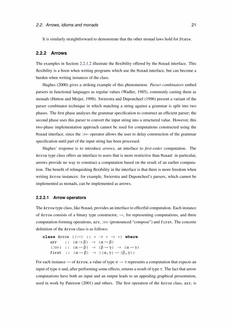
used in work by Paterson (2001) and others. The first operation of the Arrow class, arr, is
22 Chapter 2. Three models for the description of computation
analogous to the monadic return: arr creates an arrow computation from a pure function. In
the graphical presentation pure computations are denoted using circles:
f
arr f
The second operation of the Arrow class, >>>, constructs a new computation from two
existing computations, using the result of the first as the input of the second.
>>>
f g
f >>> g
The final operation of the Arrow class makes it possible to pass values from one computa-
tion to another, besides those values which are used as input to the computation.
first
f
first f
It is instructive to compare the >>> operator for arrows with the >>= operator for monads.
In both cases the result of the left operand is passed as input to the right, but whereas the right
operand of >>= constructs a computation, the right operand of >>> is a computation. Thus>>>
is (for the user of the Arrow class) less flexible than >>=, because the result of the left operand
cannot play a role in constructing the computation passed as the right operand.
The first operator for arrows fulfils a need that for monads is also met by >>=: passing
through values that are not used by intermediate computations. For example, the computation
m in Example 1 (sequencing) returns a value that is not used by the next computation, n , but
is used in the final computation. The value is bound to the variable x by the λ-abstraction
used as the continuation to m , and so the normal rules of lexical scoping bring x into scope in
the remainder of the computation. In contrast, inputs to arrow computation are not λ-bound,
so an additional operator is needed to explicitly pass through values that are needed in subse-
quent computations. (Example 5 on page 25 shows how to create an analogue of Example 1
(sequencing) using the arrow combinators.)
Several additional arrow combinators will be useful in what follows. These functions are
not part of the Arrow class since it is possible to express them in terms of the three class
2.2. Arrows, idioms and monads 23
operations. The first is second, a cognate to first, but with the difference that the additional
value is passed using the first element of the pairs in the input and output, not the second.
second
fdef=
>>>>>>
first
f
second f arr swap >>> first f >>> arr swap
Here swap is defined as the function that exchanges the elements of a pair:
swap (x,y) = (y,x)
The second combinator, ∗∗∗, builds a computation that transforms pairs from two computa-
tions, passing the first element of the pair to the first computation and the second element of
the pair to the second computation.
***
g
f
def=
>>>first
f
second
g
f ∗∗∗ g first f >>> second g
Note that the sequencing of effects places f before g . This ordering is reflected in the rela-
tive horizontal placement of the boxes in the diagram; we use the same convention throughout
this chapter.
The final combinator, &&&, is similar to the ∗∗∗ combinator, but passes the same value as
input to both computations:
&&&
g
f
def=
>>>***
g
f
f &&& g arr dup >>> (f ∗∗∗ g)
Here dup is defined as the function that takes a single value into the two elements of a pair:
dup x = (x,x)
24 Chapter 2. Three models for the description of computation
2.2.2.2 Arrow examples
The Arrow interface has been used for a wide range of applications, including parsers and
printers (Jansson and Jeuring, 1999), web interaction (Hughes, 2000), circuits (Paterson, 2001),
graphic user interfaces (Courtney and Elliott, 2001), and robotics (Hudak, Courtney, Nilsson,
and Peterson, 2003). We restrict our attention here to three simple instances. The first instance
is the “identity” arrow of pure functions, where arr is the identity function, >>> is reverse
function composition, and first applies its argument to the first element of a pair.
instance Arrow → wherearr = id
f >>> g = g · ffirst f = f × id
(We write f × g for the function λ(x,y)→ (f x,g y).)
The second instance generalises Swierstra and Duponcheel’s two-phase parsers to arbitrary
two-phase computations. We introduce a new type with four parameters: monads m and n for
the “static” and “dynamic” parts of a computation, and input and result types α and β.
newtype TwoPhase (m :: * → *) (n : * → *) α β= TwoPhase { runTwoPhase :: m (α→ n β) }
We can then write an Arrow instance for TwoPhase. A computation of type TwoPhase m n α β
accepts an input of type α and returns a result of type β. All of the effects in the “static” monad
m are performed before any of the effects in the “dynamic” monad n, and only computations
in n, not computations inm, may depend on the arrow input.
instance (Monad m, Monad n) ⇒ Arrow (TwoPhase m n) wherearr f = TwoPhase (return (return · f))TwoPhase f >>> TwoPhase g = TwoPhase (f >>= λh →
g >>= λk →return (λa → h a >>= k))
first (TwoPhase f) = TwoPhase (f >>= λh →return (λ(a,c) →
h a >>= λb →return (b,c)))
The implementation of the arr operator is a straightforward combination of the return oper-
ators of the monadsm and n. A computation of the form f >>> g uses the >>= operator ofm
to extract the dynamic portions h and k from f and g, then sequences those dynamic portions
using the>>= operator of n, passing the arrow input a as input to h and the result of h a as input
to k. Similarly, a computation of the form first f uses the >>= operator of m to extract the
dynamic portion h of f, then applies h to the first element of the arrow input (a,c), passing
2.2. Arrows, idioms and monads 25
the second element through using the strength of n5.
The third instance is a specialisation of TwoPhase, where m is the identity monad. For
each instance n of Monad, this specialisation gives us the type of Kleisli arrows of the monad
— that is, functions of the form α→ n β. We will use this instance in translating the example
computations, so it is helpful to write out the specialisation explicitly. We introduce a new
type to represent Kleisli arrows, writing Kleisli and runKleisli for the constructor and
destructor:
newtype Kleisli (n :: * → *) α β= Kleisli { runKleisli :: α → n β }
To obtain the Kleisli instance of the Arrow class we start with the TwoPhase instance and
replace the >>= and return operations of them monad with the identity operations:
instance Monad n ⇒ Arrow (Kleisli n) wherearr f = Kleisli (return · f)Kleisli f >>> Kleisli g = Kleisli (λa→ f a >>= g)first (Kleisli f) = Kleisli (λ(a,c)→ f a >>= λb→ return (b,c))
Now we can write Arrow computations using any instance of Monad. We must also con-
vert any primitive computations of the monad to arrow computations. For the monad from
Section 2.2.1.2 we must convert get and put:
get :: Kleisli (State σ) () σget = Kleisli get
put :: Kleisli (State σ) σ ()put = Kleisli put
We can now write Examples 1 (sequencing) and 2 (dataflow) as arrow computations.
Example 5 (sequencing with arrows). Sequencing computations and collecting results is
the purpose of the &&& operator. Given arrow computations m of type ()→ σ and n of type
()→ τ, the analogue of Example 1 (sequencing) may be written m &&& n .
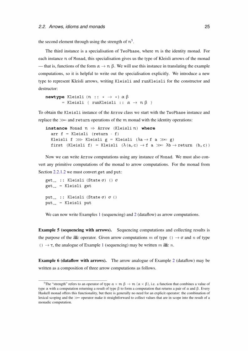
Example 6 (dataflow with arrows). The arrow analogue of Example 2 (dataflow) may be
written as a composition of three arrow computations as follows.
5The “strength” refers to an operator of type α ×m β → m (α × β), i.e. a function that combines a value oftype α with a computation returning a result of type β to form a computation that returns a pair of α and β. EveryHaskell monad offers this functionality, but there is generally no need for an explicit operator: the combination oflexical scoping and the >>= operator make it straightforward to collect values that are in scope into the result of amonadic computation.
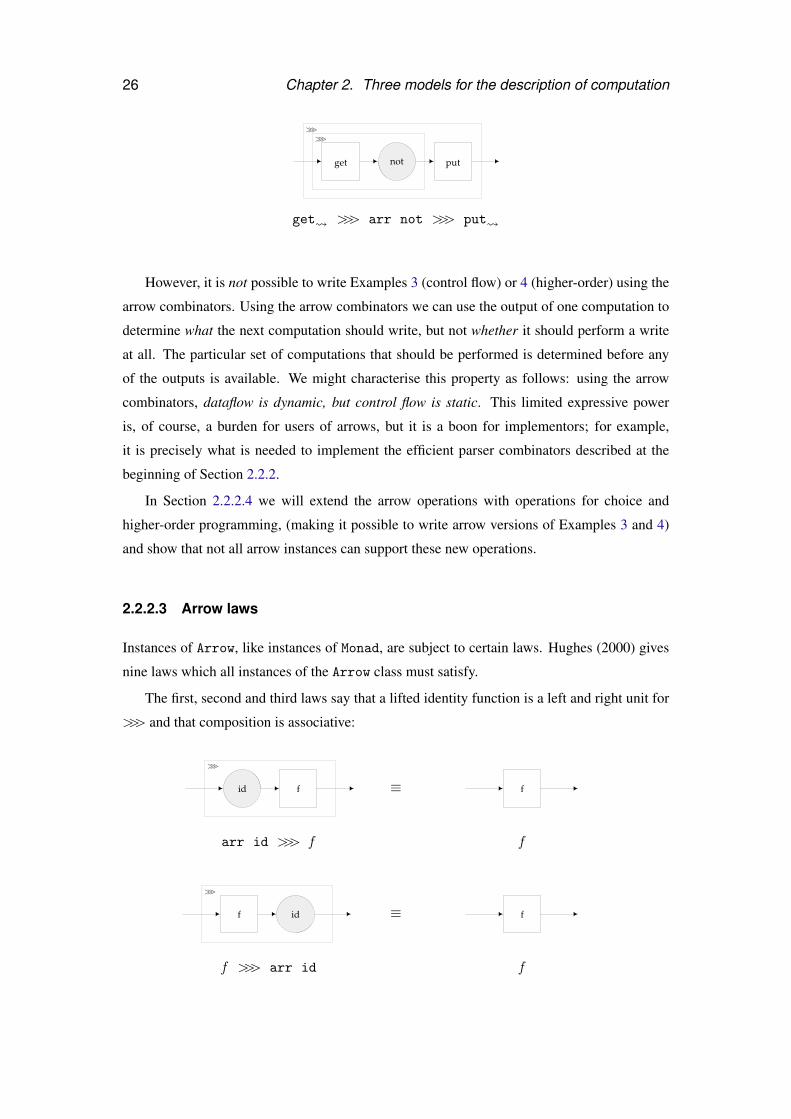
26 Chapter 2. Three models for the description of computation
>>>>>>
get not put
get >>> arr not >>> put
However, it is not possible to write Examples 3 (control flow) or 4 (higher-order) using the
arrow combinators. Using the arrow combinators we can use the output of one computation to
determine what the next computation should write, but not whether it should perform a write
at all. The particular set of computations that should be performed is determined before any
of the outputs is available. We might characterise this property as follows: using the arrow
combinators, dataflow is dynamic, but control flow is static. This limited expressive power
is, of course, a burden for users of arrows, but it is a boon for implementors; for example,
it is precisely what is needed to implement the efficient parser combinators described at the
beginning of Section 2.2.2.
In Section 2.2.2.4 we will extend the arrow operations with operations for choice and
higher-order programming, (making it possible to write arrow versions of Examples 3 and 4)
and show that not all arrow instances can support these new operations.
2.2.2.3 Arrow laws
Instances of Arrow, like instances of Monad, are subject to certain laws. Hughes (2000) gives
nine laws which all instances of the Arrow class must satisfy.
The first, second and third laws say that a lifted identity function is a left and right unit for
>>> and that composition is associative:
>>>
id f ≡ f
arr id >>> f f
>>>
idf ≡ f
f >>> arr id f
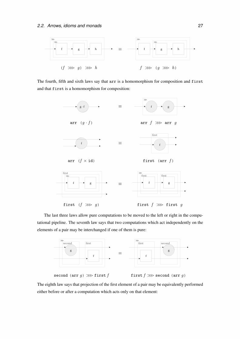
2.2. Arrows, idioms and monads 27
>>>>>>
f g h ≡
>>>>>>
f g h
(f >>> g) >>> h f >>> (g >>> h)
The fourth, fifth and sixth laws say that arr is a homomorphism for composition and first
and that first is a homomorphism for composition:
g . f ≡>>>
f g
arr (g · f ) arr f >>> arr g
f ≡
first
f
arr (f × id) first (arr f )
first>>>
f g ≡
>>>firstfirst
f g
first (f >>> g) first f >>> first g
The last three laws allow pure computations to be moved to the left or right in the compu-
tational pipeline. The seventh law says that two computations which act independently on the
elements of a pair may be interchanged if one of them is pure:
>>>second first
f
g≡
>>>first
f
second
g
second (arr g) >>> first f first f >>> second (arr g)
The eighth law says that projection of the first element of a pair may be equivalently performed
either before or after a computation which acts only on that element:
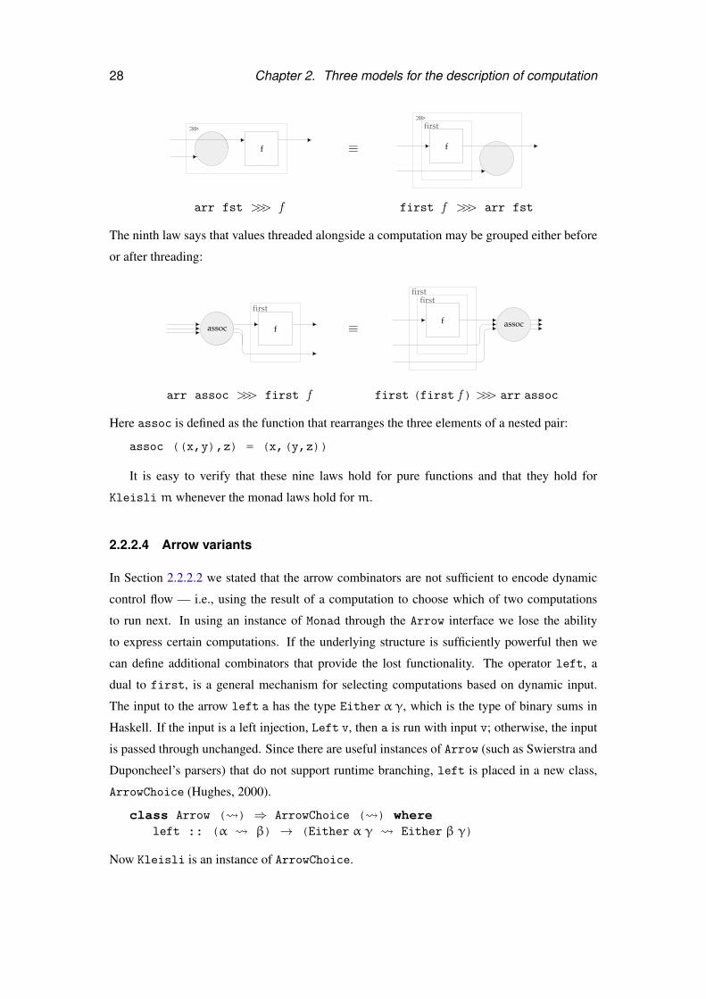
28 Chapter 2. Three models for the description of computation
>>>
f ≡
>>>first
f
arr fst >>> f first f >>> arr fst
The ninth law says that values threaded alongside a computation may be grouped either before
or after threading:
first
fassoc ≡
firstfirst
f assoc
arr assoc >>> first f first (first f ) >>> arr assoc
Here assoc is defined as the function that rearranges the three elements of a nested pair:
assoc ((x,y),z) = (x,(y,z))
It is easy to verify that these nine laws hold for pure functions and that they hold for
Kleisli m whenever the monad laws hold form.
2.2.2.4 Arrow variants
In Section 2.2.2.2 we stated that the arrow combinators are not sufficient to encode dynamic
control flow — i.e., using the result of a computation to choose which of two computations
to run next. In using an instance of Monad through the Arrow interface we lose the ability
to express certain computations. If the underlying structure is sufficiently powerful then we
can define additional combinators that provide the lost functionality. The operator left, a
dual to first, is a general mechanism for selecting computations based on dynamic input.
The input to the arrow left a has the type Either α γ, which is the type of binary sums in
Haskell. If the input is a left injection, Left v, then a is run with input v; otherwise, the input
is passed through unchanged. Since there are useful instances of Arrow (such as Swierstra and
Duponcheel’s parsers) that do not support runtime branching, left is placed in a new class,
ArrowChoice (Hughes, 2000).
class Arrow ( ) ⇒ ArrowChoice ( ) whereleft :: (α β) → (Either α γ Either β γ)
Now Kleisli is an instance of ArrowChoice.
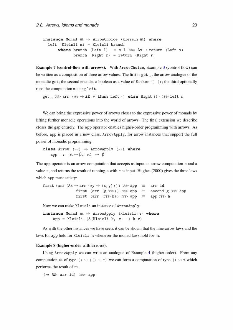
2.2. Arrows, idioms and monads 29
instance Monad m ⇒ ArrowChoice (Kleisli m) whereleft (Kleisli m) = Kleisli branch
where branch (Left l) = m l >>= λv→ return (Left v)branch (Right r) = return (Right r)
Example 7 (control-flow with arrows). With ArrowChoice, Example 3 (control flow) can
be written as a composition of three arrow values. The first is get , the arrow analogue of the
monadic get; the second encodes a boolean as a value of Either () (); the third optionally
runs the computation m using left.
get >>> arr (λv→ if v then Left () else Right ()) >>> left m
We can bring the expressive power of arrows closer to the expressive power of monads by
lifting further monadic operations into the world of arrows. The final extension we describe
closes the gap entirely. The app operator enables higher-order programming with arrows. As
before, app is placed in a new class, ArrowApply, for arrow instances that support the full
power of monadic programming.
class Arrow ( ) ⇒ ArrowApply ( ) whereapp :: (α β, α) β
The app operator is an arrow computation that accepts as input an arrow computation a and a
value v , and returns the result of running a with v as input. Hughes (2000) gives the three laws
which app must satisfy:
first (arr (λx→ arr (λy→ (x,y)))) >>> app ≡ arr id
first (arr (g >>>)) >>> app ≡ second g >>> app
first (arr (>>> h)) >>> app ≡ app >>> h
Now we can make Kleisli an instance of ArrowApply:
instance Monad m ⇒ ArrowApply (Kleislim) whereapp = Kleisli (λ(Kleisli k, v) → k v)
As with the other instances we have seen, it can be shown that the nine arrow laws and the
laws for app hold for Kleislim whenever the monad laws hold form.
Example 8 (higher-order with arrows).
Using ArrowApply we can write an analogue of Example 4 (higher-order). From any
computation m of type () (() τ) we can form a computation of type () τ which
performs the result of m .
(m &&& arr id) >>> app
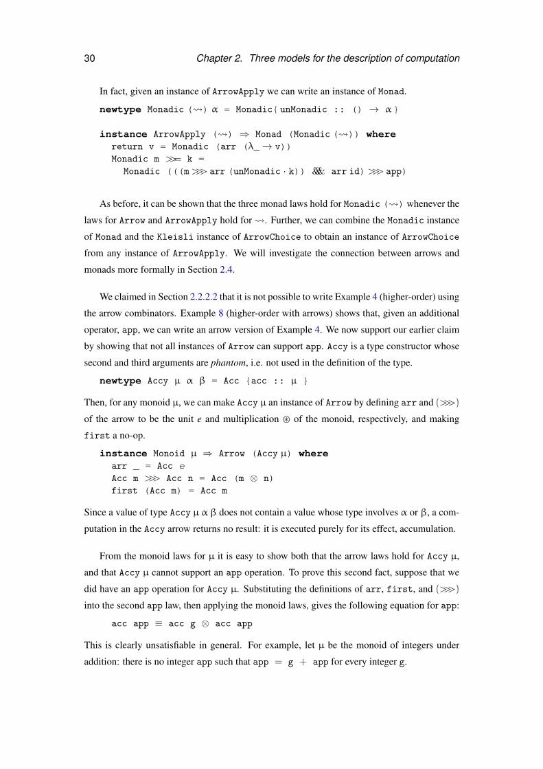
30 Chapter 2. Three models for the description of computation
In fact, given an instance of ArrowApply we can write an instance of Monad.
newtype Monadic ( ) α = Monadic{ unMonadic :: () → α}
instance ArrowApply ( ) ⇒ Monad (Monadic ( )) wherereturn v = Monadic (arr (λ_→ v))Monadic m >>= k =
Monadic (((m>>> arr (unMonadic · k)) &&& arr id)>>> app)
As before, it can be shown that the three monad laws hold for Monadic ( ) whenever the
laws for Arrow and ArrowApply hold for . Further, we can combine the Monadic instance
of Monad and the Kleisli instance of ArrowChoice to obtain an instance of ArrowChoice
from any instance of ArrowApply. We will investigate the connection between arrows and
monads more formally in Section 2.4.
We claimed in Section 2.2.2.2 that it is not possible to write Example 4 (higher-order) using
the arrow combinators. Example 8 (higher-order with arrows) shows that, given an additional
operator, app, we can write an arrow version of Example 4. We now support our earlier claim
by showing that not all instances of Arrow can support app. Accy is a type constructor whose
second and third arguments are phantom, i.e. not used in the definition of the type.
newtype Accy µ α β = Acc {acc :: µ }
Then, for any monoid µ, we can make Accy µ an instance of Arrow by defining arr and (>>>)
of the arrow to be the unit e and multiplication � of the monoid, respectively, and making
first a no-op.
instance Monoid µ ⇒ Arrow (Accy µ) wherearr _ = Acc eAcc m >>> Acc n = Acc (m ⊗ n)first (Acc m) = Acc m
Since a value of type Accy µ α β does not contain a value whose type involves α or β, a com-
putation in the Accy arrow returns no result: it is executed purely for its effect, accumulation.
From the monoid laws for µ it is easy to show both that the arrow laws hold for Accy µ,
and that Accy µ cannot support an app operation. To prove this second fact, suppose that we
did have an app operation for Accy µ. Substituting the definitions of arr, first, and (>>>)
into the second app law, then applying the monoid laws, gives the following equation for app:
acc app ≡ acc g ⊗ acc app
This is clearly unsatisfiable in general. For example, let µ be the monoid of integers under
addition: there is no integer app such that app = g + app for every integer g.
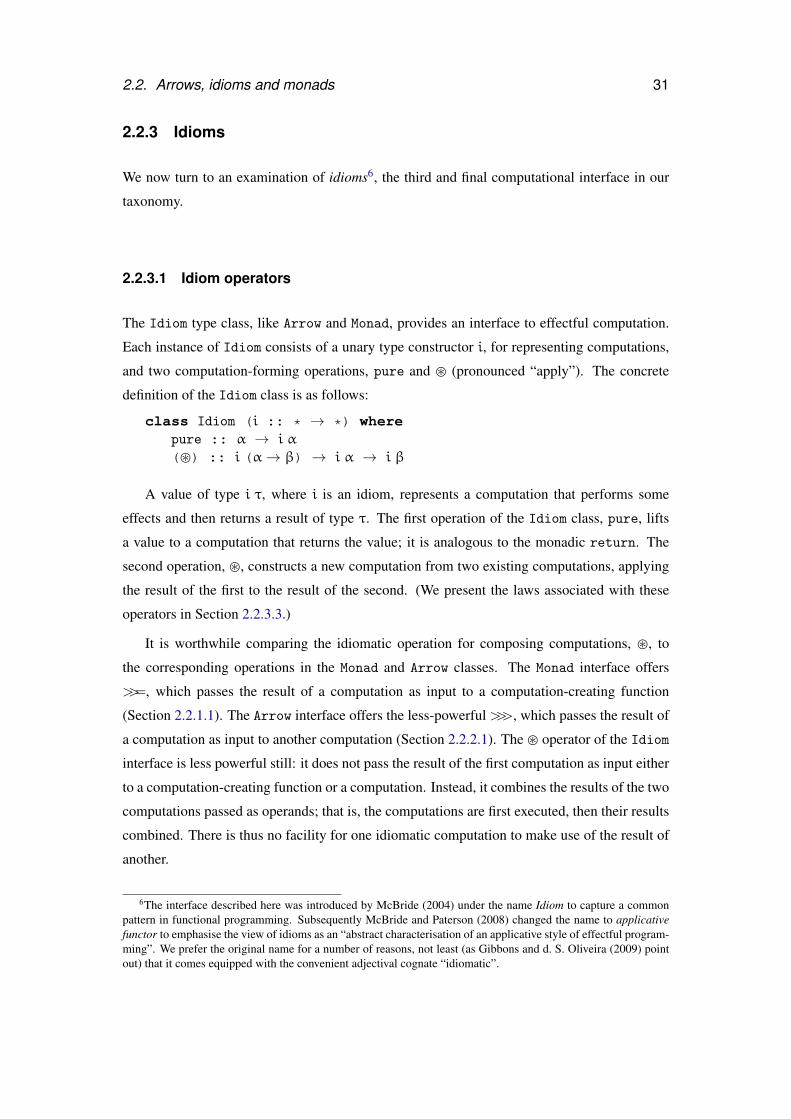
2.2. Arrows, idioms and monads 31
2.2.3 Idioms
We now turn to an examination of idioms6, the third and final computational interface in our
taxonomy.
2.2.3.1 Idiom operators
The Idiom type class, like Arrow and Monad, provides an interface to effectful computation.
Each instance of Idiom consists of a unary type constructor i, for representing computations,
and two computation-forming operations, pure and � (pronounced “apply”). The concrete
definition of the Idiom class is as follows:
class Idiom (i :: * → *) wherepure :: α → i α
(�) :: i (α→ β) → i α → i β
A value of type i τ, where i is an idiom, represents a computation that performs some
effects and then returns a result of type τ. The first operation of the Idiom class, pure, lifts
a value to a computation that returns the value; it is analogous to the monadic return. The
second operation, �, constructs a new computation from two existing computations, applying
the result of the first to the result of the second. (We present the laws associated with these
operators in Section 2.2.3.3.)
It is worthwhile comparing the idiomatic operation for composing computations, �, to
the corresponding operations in the Monad and Arrow classes. The Monad interface offers
>>=, which passes the result of a computation as input to a computation-creating function
(Section 2.2.1.1). The Arrow interface offers the less-powerful >>>, which passes the result of
a computation as input to another computation (Section 2.2.2.1). The � operator of the Idiom
interface is less powerful still: it does not pass the result of the first computation as input either
to a computation-creating function or a computation. Instead, it combines the results of the two
computations passed as operands; that is, the computations are first executed, then their results
combined. There is thus no facility for one idiomatic computation to make use of the result of
another.
6The interface described here was introduced by McBride (2004) under the name Idiom to capture a commonpattern in functional programming. Subsequently McBride and Paterson (2008) changed the name to applicativefunctor to emphasise the view of idioms as an “abstract characterisation of an applicative style of effectful program-ming”. We prefer the original name for a number of reasons, not least (as Gibbons and d. S. Oliveira (2009) pointout) that it comes equipped with the convenient adjectival cognate “idiomatic”.
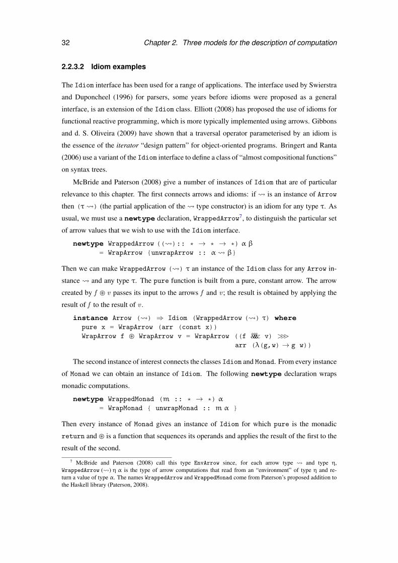
32 Chapter 2. Three models for the description of computation
2.2.3.2 Idiom examples
The Idiom interface has been used for a range of applications. The interface used by Swierstra
and Duponcheel (1996) for parsers, some years before idioms were proposed as a general
interface, is an extension of the Idiom class. Elliott (2008) has proposed the use of idioms for
functional reactive programming, which is more typically implemented using arrows. Gibbons
and d. S. Oliveira (2009) have shown that a traversal operator parameterised by an idiom is
the essence of the iterator “design pattern” for object-oriented programs. Bringert and Ranta
(2006) use a variant of the Idiom interface to define a class of “almost compositional functions”
on syntax trees.
McBride and Paterson (2008) give a number of instances of Idiom that are of particular
relevance to this chapter. The first connects arrows and idioms: if is an instance of Arrow
then (τ ) (the partial application of the type constructor) is an idiom for any type τ. As
usual, we must use a newtype declaration, WrappedArrow7, to distinguish the particular set
of arrow values that we wish to use with the Idiom interface.
newtype WrappedArrow (( ):: * → * → *) α β= WrapArrow {unwrapArrow :: α β}
Then we can make WrappedArrow ( ) τ an instance of the Idiom class for any Arrow in-
stance and any type τ. The pure function is built from a pure, constant arrow. The arrow
created by f � v passes its input to the arrows f and v ; the result is obtained by applying the
result of f to the result of v .
instance Arrow ( ) ⇒ Idiom (WrappedArrow ( ) τ) wherepure x = WrapArrow (arr (const x))WrapArrow f � WrapArrow v = WrapArrow ((f &&& v) >>>
arr (λ(g,w)→ g w))
The second instance of interest connects the classes Idiom and Monad. From every instance
of Monad we can obtain an instance of Idiom. The following newtype declaration wraps
monadic computations.
newtype WrappedMonad (m :: * → *) α= WrapMonad { unwrapMonad :: m α }
Then every instance of Monad gives an instance of Idiom for which pure is the monadic
return and � is a function that sequences its operands and applies the result of the first to the
result of the second.
7 McBride and Paterson (2008) call this type EnvArrow since, for each arrow type and type η,WrappedArrow ( ) η α is the type of arrow computations that read from an “environment” of type η and re-turn a value of type α. The names WrappedArrow and WrappedMonad come from Paterson’s proposed addition tothe Haskell library (Paterson, 2008).
2.2. Arrows, idioms and monads 33
instance Monad m ⇒ Idiom (WrappedMonad m) wherepure v = WrapMonad (return v)WrapMonad f � WrapMonad v = WrapMonad (f >>= λg→
v >>= λw→return (g w))
The third instance of interest makes it possible to build new instances of Idiom from exist-
ing instances by straightforward functor composition. The type constructor Compose composes
two functors.
newtype Compose (i :: * → *) (j :: * → *) α= Compose { deCompose :: i (j α) }
The definition of the Idiom instance for Compose simply lifts the pure and � of the inner
idiom to the outer idiom.
instance (Idiom i, Idiom j) ⇒ Idiom (Compose i j) wherepure v = Compose (pure (pure v))Compose f � Compose v = Compose (pure (�) � f � v)
A further instance of Idiom will be useful in exploring the connections with Arrow and
Monad. The environment idiom captures the effect of reading from (constant) input. We can
define the environment idiom in Haskell using the pure function arrow, partially applied to any
input type τ.
instance Idiom ((→) τ) wherepure v = λe→ v
f � v = λe→ f e (v e)
This instance is isomorphic to the instance obtained by instantiating the arrow parameter of
WrappedArrow to→, the type of pure functions, and to the instance obtained by instantiating
the monad parameter of WrappedMonad to the environment monad (which is called Reader in
the Haskell standard library).
We now have two ways to obtain an instance of Idiom from an instance m of Monad. The
first way is direct: simply apply WrappedMonad. The second way is indirect: apply Kleisli
to obtain an instance of Arrow and then apply WrappedArrow to obtain an instance of Idiom.
Ignoring the isomorphisms introduced by the various newtype declarations, this latter method
results in the type τ→ m α (for the result type α), which is not equivalent to the type m α
obtained using the direct method. We can therefore obtain at least two distinct instances of
Idiom from any instance of Monad. However, it is easy to convert either instance into the
other. The instance obtained with WrappedMonad may be converted into the instance obtained
with WrappedArrow by composition with the environment idiom. The instance obtained with
WrappedArrow may be converted into an instance isomorphic to the instance obtained with
34 Chapter 2. Three models for the description of computation
WrappedMonad by instantiating τ to the unit type.
McBride and Paterson (2008) give one final instance that connects Arrow and Idiom. For
any Idiom instance i, StaticArrow i is an arrow transformer that uses an idiomatic compu-
tation to construct an arrow computation.
newtype StaticArrow (i :: * → *) (( ) :: * → * → *) α β= Static { exStatic :: i (α β) }
The arrangement of the type constructors dictates that all of the effects of the idiom occur before
any of the effects of the arrow. The definitions of the Arrow methods for StaticArrow i ( )
are then the simply operations of the arrow lifted into the idiom i: arr creates a pure id-
iomatic computation that returns a pure arrow computation; f >>> g runs the idiomatic com-
putations f and g , passing the results to the >>> operator of the underlying arrow; first f
runs the idiomatic computation f and applies the first operator of the underlying arrow to
the result.
instance (Idiom i,Arrow ( ))⇒ Arrow (StaticArrow i ( )) wherearr f = Static (pure (arr f))Static f >>> Static g = Static (pure (>>>) � f � g)first (Static f) = Static (pure first � f)
We now have two ways to obtain an instance of Arrow from an instance m of Monad. The
first way is direct: simply apply Kleisli. The second way is indirect: apply WrappedMonad
to obtain an instance of Idiom and then apply StaticArrow (with the arrow parameter in-
stantiated to the pure function arrow, →) to obtain an instance of Arrow. Ignoring the iso-
morphisms introduced by the various newtype declarations, this latter method results in the
type m (α→ β) (for input type α and result type β), which is generally not equivalent to
the type α→ m β obtained using the direct method. We can therefore obtain at least two dis-
tinct instances of Arrow from any instance of Monad. This time there is no general conversion
procedure between the two. However, two approaches do yield equivalent results for certain
monads. For the environment monad (where m α ' τ → α), the two approaches result in
arrows that are isomorphic.
Using the idiom operators we can write a program analogous to Example 1 (sequencing)
for sequencing two computations.
Example 9 (sequencing with idioms).
Suppose m and n are idiomatic computations with the types i σ and i τ respectively. Then
the following computation of type i (σ, τ) executes m and n in order and returns the results
as a pair.
2.2. Arrows, idioms and monads 35
pure (λx y→ (x,y)) � m � n
However, there is no way to write idiomatic analogues of any of the programs in Examples 2
(dataflow), 3 (control flow) or 4 (higher-order).
In Section 2.2.2.2 we characterised arrow computations as having dynamic dataflow, but
static control flow. This is manifested in our examples of state-passing as the ability to decide
what to write based on the result of a prior computation, but not whether to write. The expres-
sive power offered by the Idiom interface is even more limited: there is no way at all to pass
the result of one computation as input to another computation. With idioms, therefore, there is
no means to construct a state-passing computation that uses a prior result either to determine
whether to perform a write or to determine what to write. We might characterise this property
as follows: using the idiom combinators, both dataflow and control flow are static.
In Section 2.2.2.4 we used the Accy phantom monoid accumulator instance of Arrow to
show that not all arrows supported app. We will use a similar instance for Idioms (first intro-
duced by McBride and Paterson) to show that the Idiom operations alone cannot support the
operation needed to implement Example 4.
The AccI type constructor takes two arguments, using only the first in its definition.
newtype AccI µ α = AccI {acci :: µ }
The Idiom instance for AccI µ is constructed by defining pure and � to be the unit e and
multiplication ⊗ of the monoid µ, respectively. (We could obtain an equivalent instance by
combining the WrappedArrow instance given earlier with the Accy instance of Arrow.)
instance Monoid µ ⇒ Idiom (AccI µ) wherepure _ = AccI eAccI m � AccI n = AccI (m ⊗ n)
Now, if AccI supported the monad multiplication operator (commonly called join), then it
would necessarily satisfy the following law, which holds for all monads:
join (pure x) ≡ x
However, since the AccI definition of pure discards its argument, this law cannot be satisfied.
2.2.3.3 Idiom laws
The Idiom interface, like Monad and Arrow, comes with a number of laws which must be
satisfied by every instance.
The first law says that pure is a homomorphism for application.
36 Chapter 2. Three models for the description of computation
pure (f v) ≡ pure f � pure v
The second law says that a lifted identity function is a left unit for idiomatic application.
u ≡ pure id � u
The third law says that nested applications can be flattened using a lifted composition operation.
u � (v � w) ≡ pure (·) � u � v � w
The fourth law says that pure computations can be moved to the left or right of other computa-
tions.
v � pure x ≡ pure (λf→ f x) � v
(We observe that the latter three laws correspond to three combinators — I, B, and C — that
form a basis for linear combinatory logic. The fourth law does not contain the C combinator
directly, but is equivalent to a (less elegant) law which does:
f � u � pure x ≡ pure flip � f � pure x � u
(Here flip is the Haskell name for the C combinator: flip f x y = f y x.) This law follows
from the four idiom laws; conversely, the fourth idiom law follows from the first three idiom
laws and this law.)
It is straightforward to show that for each of the instances in Section 2.2.3.2 these four
laws follow from the laws on the underlying structures — for example, that the idiom laws
for WrappedMonad m follow from the monad laws hold for m and that the idiom laws for
WrappedArrow ( ) follow from the arrow laws for .
2.2.3.4 Sundries
We have seen that an idiom computation is composed of independent sub-computations whose
results are combined to give the final output (Section 2.2.5.3). In particular, no sub-computation
may make use of the result of another sub-computation. This independence leads to consider-
able freedom in writing idiom instances, exemplified in the following idiom transformer. The
Mirror transformer converts any idiom i to an idiom Mirror i which reverses the sequence of
effects of i. At the type level, Mirror is the identity:
newtype Mirror (i :: * → *) α = Mirror (i α)
The definition of pure is similarly trivial. The � operator for Mirror exchanges the order of
the operands, and applies the result of the second to the result of the first.
instance Idiom i ⇒ Idiom (Mirror i) wherepure f = Mirror (pure f)Mirror f � Mirror p = Mirror (pure (flip ($)) � p � f)
2.2. Arrows, idioms and monads 37
(Here $ denotes the identity function at function type.)
It is straightforward to check that the idiom laws for Mirror i follow from the idiom laws
for i.
2.2.4 Monoids
The reader might also wonder whether there are any further computational interfaces in the
progression. Monadic computations may be dynamic both in dataflow and control flow. Arrows
fix control flow statically, but retain dynamic dataflow; idioms introduce the restriction that
dataflow must also be statically fixed. A natural question to ask is whether the fourth point in
this matrix has any interesting occupants: that is, whether we might usefully define a class for
capturing computations where control flow is dynamic, but dataflow is static. We will not give
a definitive answer to this question, but note that it appears to be difficult to introduce operators
for dynamic control flow without making dataflow dynamic also. For example we can define
a new class DynamicIdiom which adds a facility to the Idiom interface for branching on the
result of a computation:
class Idiom i ⇒ DynamicIdiom i wherebranch :: i Bool → i α → i α → i α
Now the branch operation makes it possible to write both Example 3 (control flow):
branch (WrapMonad (get ())) m (pure ())
and Example 2 (dataflow):
branch (WrapMonad (get ()))(WrapMonad (put False))(WrapMonad (put True))
Rather than pursue this question further we will consider what further restrictions we could
introduce. One possibility is to remove the capacity for a computation to yield a result; this
takes us from idioms to monoids. A monoidal effectful computation is simply a sequence of
effectful subcomputations with fixed control flow, fixed dataflow, and no result. We saw in
Section 2.2.3.2 that fixing the input parameter of an arrow yields an idiom. Similarly, fixing
the output parameter of an idiom yields a monoid. In Haskell the Monoid type class is defined
as follows:
class Monoid µ wheree :: µ
(⊗) :: µ → µ → µ
We can construct a monoid from an idiom i by applying i to the unit type.
38 Chapter 2. Three models for the description of computation
newtype Muffled :: (i :: * → *) = Muffle (i ())
The e value is obtained by lifting the unit value, (). The implementation of ⊗ combines its
operands using � and uses a lifted constant function to discard the result.
instance Idiom i ⇒ Monoid (Muffled i) wheree = Muffle (pure ())Muffle f ⊗ Muffle p = Muffle (pure (λ_ _→ ()) � f � p)
It is straightforward to check that the monoid laws for Muffled i (i.e. that ⊗ is associative
with e as left and right unit) follow from the idiom laws for i.
An auxiliary function, muffle, replaces the result of any idiomatic computation with the
unit value, making the computation available for use in the monoid:
muffle :: Idiom i ⇒ i α → Muffled i
muffle i = pure (λ_→ ()) � i
Section 2.2.3.2 showed how to obtain an instance AccI µ of Idiom for any Monoid instance
µ. Using Muffled we can recover the original Monoid instance from AccI. That is, the
Monoid instance for Muffled (AccI µ) is equivalent to the Monoid instance for µ.
Example 10 (sequencing with monoids).
If m and n are computations of type i σ and i τ respectively (for some Idiom instance i)
then the following monoidal computation executes m and n in order, discarding their results.
muffle m ⊗ muffle n
2.2.5 Normal forms
The laws which accompany the idiom, arrow and monad interfaces group computations into
equivalence classes. Any particular computation can be expressed equivalently using any mem-
ber of its class. For example, if we wish to nest occurrences of the >>> operator in an arrow
computation, the third arrow law gives us the choice whether to group to the left (writing
(f >>> g) >>> h) or to the right (writing f >>> (g >>> h)). On occasion we may wish to
check whether two computations belong to the same equivalence class. One way to answer this
question is to attempt to find some way to rewrite one of the computations into the other by
repeatedly applying laws.
Determining equivalence is much more convenient if we choose a canonical member of
each equivalence class and define a normalisation procedure for obtaining the canonical mem-
ber from any computation. Determining whether two computations are equivalent then be-
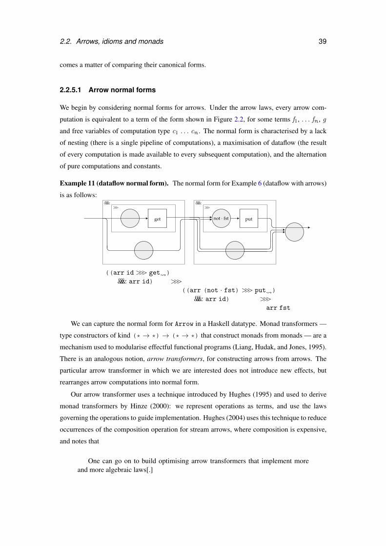
2.2. Arrows, idioms and monads 39
comes a matter of comparing their canonical forms.
2.2.5.1 Arrow normal forms
We begin by considering normal forms for arrows. Under the arrow laws, every arrow com-
putation is equivalent to a term of the form shown in Figure 2.2, for some terms f1, . . . fn, g
and free variables of computation type c1 . . . cn. The normal form is characterised by a lack
of nesting (there is a single pipeline of computations), a maximisation of dataflow (the result
of every computation is made available to every subsequent computation), and the alternation
of pure computations and constants.
Example 11 (dataflow normal form). The normal form for Example 6 (dataflow with arrows)
is as follows:&&&
>>>
get
&&&>>>
not fst. put
((arr id >>> get )&&& arr id) >>>
((arr (not · fst) >>> put )&&& arr id) >>>
arr fst
We can capture the normal form for Arrow in a Haskell datatype. Monad transformers —
type constructors of kind (*→ *)→ (*→ *) that construct monads from monads — are a
mechanism used to modularise effectful functional programs (Liang, Hudak, and Jones, 1995).
There is an analogous notion, arrow transformers, for constructing arrows from arrows. The
particular arrow transformer in which we are interested does not introduce new effects, but
rearranges arrow computations into normal form.
Our arrow transformer uses a technique introduced by Hughes (1995) and used to derive
monad transformers by Hinze (2000): we represent operations as terms, and use the laws
governing the operations to guide implementation. Hughes (2004) uses this technique to reduce
occurrences of the composition operation for stream arrows, where composition is expensive,
and notes that
One can go on to build optimising arrow transformers that implement moreand more algebraic laws[.]
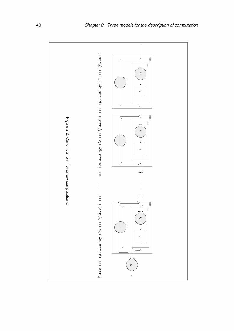
40 Chapter 2. Three models for the description of computation
&&&>>>
f1
c1
&&&>>>
f2
c2
&&&>>>
fn
cn
g
((arrf1>>>
c1 )
&&&arrid)>>>
((arrf2>>>
c2 )
&&&arrid)>>>
...>>>
((arrfn>>>
cn)
&&&arrid)>>>
arrg
Figure2.2:
Canonicalform
forarrowcom
putations.
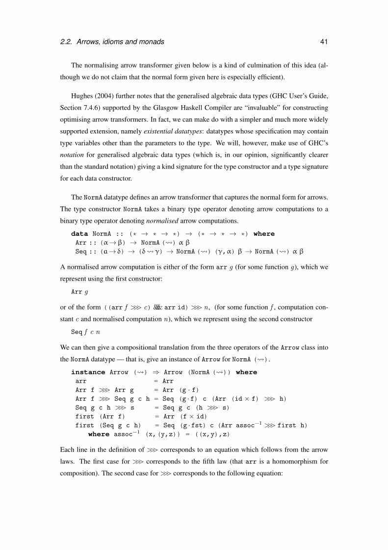
2.2. Arrows, idioms and monads 41
The normalising arrow transformer given below is a kind of culmination of this idea (al-
though we do not claim that the normal form given here is especially efficient).
Hughes (2004) further notes that the generalised algebraic data types (GHC User’s Guide,
Section 7.4.6) supported by the Glasgow Haskell Compiler are “invaluable” for constructing
optimising arrow transformers. In fact, we can make do with a simpler and much more widely
supported extension, namely existential datatypes: datatypes whose specification may contain
type variables other than the parameters to the type. We will, however, make use of GHC’s
notation for generalised algebraic data types (which is, in our opinion, significantly clearer
than the standard notation) giving a kind signature for the type constructor and a type signature
for each data constructor.
The NormA datatype defines an arrow transformer that captures the normal form for arrows.
The type constructor NormA takes a binary type operator denoting arrow computations to a
binary type operator denoting normalised arrow computations.
data NormA :: (* → * → *) → (* → * → *) whereArr :: (α→β) → NormA( ) α βSeq :: (a→ δ) → (δ γ) → NormA( ) (γ,α) β → NormA( ) α β
A normalised arrow computation is either of the form arr g (for some function g), which we
represent using the first constructor:
Arr g
or of the form ((arr f >>> c) &&& arr id)>>> n , (for some function f , computation con-
stant c and normalised computation n), which we represent using the second constructor
Seq f c n
We can then give a compositional translation from the three operators of the Arrow class into
the NormA datatype — that is, give an instance of Arrow for NormA ( ).
instance Arrow ( ) ⇒ Arrow (NormA ( )) wherearr = Arr
Arr f >>> Arr g = Arr (g · f)Arr f >>> Seq g c h = Seq (g · f) c (Arr (id × f) >>> h)Seq g c h >>> s = Seq g c (h >>> s)first (Arr f) = Arr (f × id)first (Seq g c h) = Seq (g · fst) c (Arr assoc−1 >>> first h)
where assoc−1 (x,(y,z)) = ((x,y),z)
Each line in the definition of >>> corresponds to an equation which follows from the arrow
laws. The first case for >>> corresponds to the fifth law (that arr is a homomorphism for
composition). The second case for >>> corresponds to the following equation:
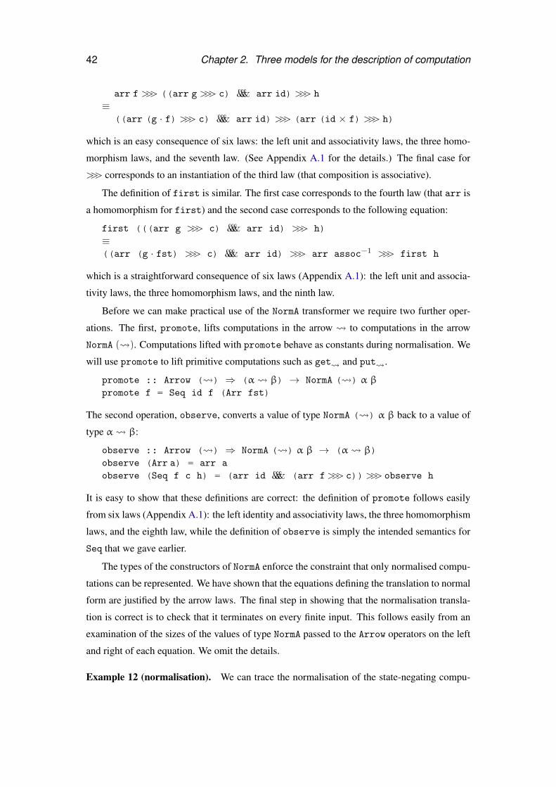
42 Chapter 2. Three models for the description of computation
arr f >>> ((arr g >>> c) &&& arr id) >>> h
≡((arr (g · f) >>> c) &&& arr id) >>> (arr (id × f) >>> h)
which is an easy consequence of six laws: the left unit and associativity laws, the three homo-
morphism laws, and the seventh law. (See Appendix A.1 for the details.) The final case for
>>> corresponds to an instantiation of the third law (that composition is associative).
The definition of first is similar. The first case corresponds to the fourth law (that arr is
a homomorphism for first) and the second case corresponds to the following equation:
first (((arr g >>> c) &&& arr id) >>> h)≡((arr (g · fst) >>> c) &&& arr id) >>> arr assoc−1 >>> first h
which is a straightforward consequence of six laws (Appendix A.1): the left unit and associa-
tivity laws, the three homomorphism laws, and the ninth law.
Before we can make practical use of the NormA transformer we require two further oper-
ations. The first, promote, lifts computations in the arrow to computations in the arrow
NormA ( ). Computations lifted with promote behave as constants during normalisation. We
will use promote to lift primitive computations such as get and put .
promote :: Arrow ( ) ⇒ (α β) → NormA ( ) α βpromote f = Seq id f (Arr fst)
The second operation, observe, converts a value of type NormA ( ) α β back to a value of
type α β:
observe :: Arrow ( ) ⇒ NormA ( ) α β → (α β)observe (Arr a) = arr a
observe (Seq f c h) = (arr id &&& (arr f>>> c))>>> observe h
It is easy to show that these definitions are correct: the definition of promote follows easily
from six laws (Appendix A.1): the left identity and associativity laws, the three homomorphism
laws, and the eighth law, while the definition of observe is simply the intended semantics for
Seq that we gave earlier.
The types of the constructors of NormA enforce the constraint that only normalised compu-
tations can be represented. We have shown that the equations defining the translation to normal
form are justified by the arrow laws. The final step in showing that the normalisation transla-
tion is correct is to check that it terminates on every finite input. This follows easily from an
examination of the sizes of the values of type NormA passed to the Arrow operators on the left
and right of each equation. We omit the details.
Example 12 (normalisation). We can trace the normalisation of the state-negating compu-
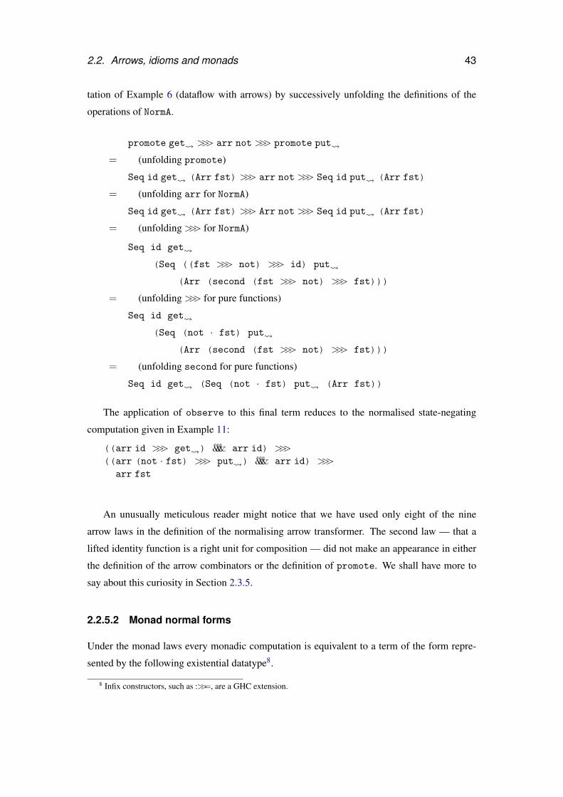
2.2. Arrows, idioms and monads 43
tation of Example 6 (dataflow with arrows) by successively unfolding the definitions of the
operations of NormA.
promote get >>> arr not >>> promote put
= (unfolding promote)
Seq id get (Arr fst) >>> arr not >>> Seq id put (Arr fst)
= (unfolding arr for NormA)
Seq id get (Arr fst) >>> Arr not >>> Seq id put (Arr fst)
= (unfolding >>> for NormA)
Seq id get
(Seq ((fst >>> not) >>> id) put
(Arr (second (fst >>> not) >>> fst)))
= (unfolding >>> for pure functions)
Seq id get
(Seq (not · fst) put
(Arr (second (fst >>> not) >>> fst)))
= (unfolding second for pure functions)
Seq id get (Seq (not · fst) put (Arr fst))
The application of observe to this final term reduces to the normalised state-negating
computation given in Example 11:
((arr id >>> get ) &&& arr id) >>>
((arr (not · fst) >>> put ) &&& arr id) >>>
arr fst
An unusually meticulous reader might notice that we have used only eight of the nine
arrow laws in the definition of the normalising arrow transformer. The second law — that a
lifted identity function is a right unit for composition — did not make an appearance in either
the definition of the arrow combinators or the definition of promote. We shall have more to
say about this curiosity in Section 2.3.5.
2.2.5.2 Monad normal forms
Under the monad laws every monadic computation is equivalent to a term of the form repre-
sented by the following existential datatype8.
8 Infix constructors, such as :>>=, are a GHC extension.
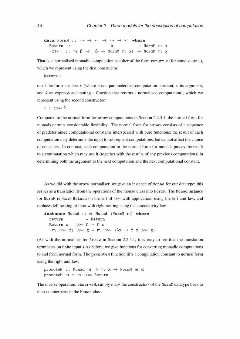
44 Chapter 2. Three models for the description of computation
data NormM :: (* → *) → (* → *) whereReturn :: α → NormM m α
(:>>=) :: m β → (β → NormM m α) → NormM m α
That is, a normalised monadic computation is either of the form return v (for some value v ),
which we represent using the first constructor:
Return v
or of the form c v >>= k (where c is a parameterised computation constant, v its argument,
and k an expression denoting a function that returns a normalised computation), which we
represent using the second constructor:
c v :>>= k
Compared to the normal form for arrow computations in Section 2.2.5.1, the normal form for
monads permits considerable flexibility. The normal form for arrows consists of a sequence
of predetermined computational constants interspersed with pure functions; the result of each
computation may determine the input to subsequent computations, but cannot affect the choice
of constants. In contrast, each computation in the normal form for monads passes the result
to a continuation which may use it (together with the results of any previous computations) in
determining both the argument to the next computation and the next computational constant.
As we did with the arrow normaliser, we give an instance of Monad for our datatype; this
serves as a translation from the operations of the monad class into NormM. The Monad instance
for NormM replaces Return on the left of >>= with application, using the left unit law, and
replaces left nesting of :>>= with right nesting using the associativity law.
instance Monad m ⇒ Monad (NormM m) wherereturn = Return
Return x >>= f = f x
(m :>>= f) >>= g = m :>>= (λx → f x >>= g)
(As with the normaliser for Arrow in Section 2.2.5.1, it is easy to see that the translation
terminates on finite input.) As before, we give functions for converting monadic computations
to and from normal form. The promoteM function lifts a computation constant to normal form
using the right unit law.
promoteM :: Monad m ⇒ m α → NormM m α
promoteM m = m :>>= Return
The inverse operation, observeM, simply maps the constructors of the NormM datatype back to
their counterparts in the Monad class.
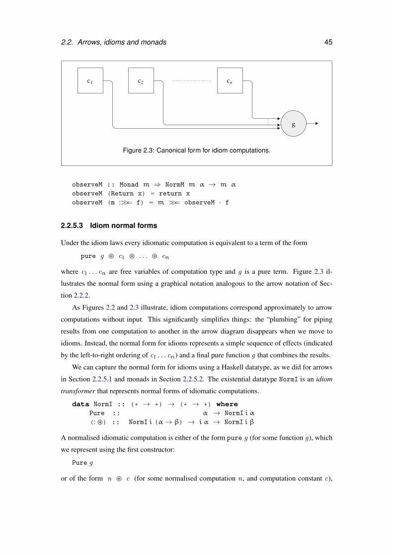
2.2. Arrows, idioms and monads 45
c1 cnc2
g
Figure 2.3: Canonical form for idiom computations.
observeM :: Monad m ⇒ NormM m α → m α
observeM (Return x) = return x
observeM (m :>>= f) = m >>= observeM · f
2.2.5.3 Idiom normal forms
Under the idiom laws every idiomatic computation is equivalent to a term of the form
pure g � c1 � . . . � cn
where c1 . . . cn are free variables of computation type and g is a pure term. Figure 2.3 il-
lustrates the normal form using a graphical notation analogous to the arrow notation of Sec-
tion 2.2.2.
As Figures 2.2 and 2.3 illustrate, idiom computations correspond approximately to arrow
computations without input. This significantly simplifies things: the “plumbing” for piping
results from one computation to another in the arrow diagram disappears when we move to
idioms. Instead, the normal form for idioms represents a simple sequence of effects (indicated
by the left-to-right ordering of c1 . . . cn) and a final pure function g that combines the results.
We can capture the normal form for idioms using a Haskell datatype, as we did for arrows
in Section 2.2.5.1 and monads in Section 2.2.5.2. The existential datatype NormI is an idiom
transformer that represents normal forms of idiomatic computations.
data NormI :: (* → *) → (* → *) wherePure :: α → NormI i α
(: �) :: NormI i (α→ β) → i α → NormI i β
A normalised idiomatic computation is either of the form pure g (for some function g), which
we represent using the first constructor:
Pure g
or of the form n � c (for some normalised computation n , and computation constant c),
46 Chapter 2. Three models for the description of computation
which we represent using the second constructor:
n : � c
We can then give an instance of Idiom for NormI i, which serves as a translation from the two
operators of the Idiom class into the NormI datatype.
instance Idiom i ⇒ Idiom (NormI i) wherepure = Pure
Pure f � Pure x = Pure (f x)u � v : � w = (Pure (·) � u � v) : � w
u � Pure x = Pure (λf→ f x) � u
It is particularly easy to see that our definition is justified by the idiom laws. The three lines of
the definition of � correspond directly to the first, third and fourth laws of Section 2.2.3.3.
As with Arrow and Monad, we need two further operations. The first, promoteI, lifts a
constant to a normalised computation.
promoteI :: Idiom i ⇒ i α → NormI i α
promoteI i = Pure id : � i
The definition of promoteI corresponds directly to the second law of Section 2.2.3.3. The
second operation, observeI, directly encodes the desired semantics of the normal form.
observeI :: Idiom i ⇒ NormI i α → i α
observeI (Pure v) = pure v
observeI (f : � v) = observeI f � v
As with the normalising arrow transformer of Section 2.2.5.1, it remains only to check that
the idiomatic normalisation translation given above terminates on all finite input. As before,
this is easy to show by tracking the sizes of the values of type NormI passed to � on the left
and right of each equation, and we omit the details.
2.2.5.4 Monoid normal forms
Under the monoid laws every monoidal computation is equivalent to a term of the form
c1 ⊗ (c2 ⊗ . . . (cn ⊗ e))
where c1 . . . cn are free variables of computation type.
We can capture the normal form for monoids using a datatype, as we did for arrows, idioms
and monads. The datatype NormMon is a monoid transformer that represents normal forms of
monoidal computations. We do not need an existential type on this occasion, since monoid
computations are not parameterised; nevertheless, we retain the GADT notation for consistency
with the other examples.
2.3. Two views of arrows 47
data NormMon :: * → * whereE :: NormMon m
(:⊗) :: m → NormMon m → NormMon m
The Monoid instance for NormMon translates the two monoid operators into the NormMon
datatype, removing occurrences of E on the left using the left-unit law and replacing left nesting
with right nesting using the associativity law.
instance Monoid m ⇒ Monoid (NormMon m) wheree = E
E ⊗ m = m
(m :⊗ n) ⊗ o = m :⊗ (n ⊗ o)
The promoteMon lifts a computation constant to normal form, using the right-unit law.
promoteMon :: Monoid m ⇒ m → NormMon m
promoteMon m = m ⊗ E
The inverse operation, observeMon, simply maps the constructors of NormMon back to their
counterparts in the Monoid class.
observeMon :: Monoid m ⇒ NormMon m → m
observeMon E = eobserveMon (m :⊗ n) = m ⊗ observeMon n
2.3 Two views of arrows9
Section 2.2 presented three interfaces to computation in decreasing order of strength: mon-
ads embed higher-order effectful computation in a functional language; arrows are restricted
to computation in which control flow is statically determined; idioms introduce the further
restriction that one computation may not make use of the result of another.
The examples of Section 2.2 illustrate the relative strength of Haskell manifestations of
monads, arrows and idioms. The normal forms of Section 2.2.5 reveal the types of computa-
tions expressible using those interfaces. Haskell is a convenient vehicle with which to explore
the various interfaces: it is the language in which each was first introduced as a program struc-
turing technique. Further, the type class system makes it convenient to give a common interface
to several notions of computation within a single program. The Haskell presentation, however,
has the unfortunate property that the interfaces differ not only semantically (which is crucial)
but notationally (which is irrelevant). For instance, the Arrow class enforces a point-free style
of programming based on composition rather than application (this is the notation), which is
limited to expressing computations for which, to repeat the slogan of Section 2.2.2.2, “dataflow
9This section is a revision of Lindley et al. (2008a).
48 Chapter 2. Three models for the description of computation
is dynamic, but control flow is static” (this is the semantics). These aspects are essentially in-
dependent: there is nothing inherently point-free about static control flow. Likewise for Idiom:
the notation is applicative, but this is hardly essential. (Indeed, McBride and Paterson (2008)
give an alternative presentation of idioms as lax monoidal functors.) A more semantic charac-
terisation of idioms is that “both dataflow and control flow are static”; this has little or nothing
to do with the applicative style.
In the following pages we will use an alternative formulation which avoids irrelevant dif-
ferences of notation, making it easier to compare expressive power directly. Our approach is
to show that idioms and monads correspond to static and higher-order variations on a metalan-
guage for arrow computations, the arrow calculus. We will use this metalanguage to reveal the
formal relationships between the three interfaces, justifying the informal claims of Section 2.2.
2.3.1 Classic arrows
We refer to the presentation of arrows given in Section 2.2.2 as classic arrows.
We present both classic arrows and arrow calculus as equational theories, which are defined
as follows.
Definition 1. A typed equational theory T consists of the following
• variables x, y, z
• types A,B,C
• terms L,M,N
• type environments Γ ::= · | x : A, Γ
• typing judgments Γ `T M : A
• equational judgments Γ `T M = N : A
Equational judgments must be well-formed: if Γ `T M = N : A then Γ `T M : A and
Γ `T N : A. We present the equational judgments via laws relating terms, writing M = N as
shorthand for Γ `T M = N : A for all Γ ,A in T such that Γ `T M : A and Γ `T N : A. The
equational theory is defined as the contextual and equivalence closure of the laws.
Figure 2.4 (page 50) gives a standard definition of the theory of typed lambda calculus
extended with pairs and unit, λ→×1. A type judgment Γ `M : A indicates that in environment
Γ term M has type A. We use a Curry formulation, eliding types from terms. Products and
functions satisfy beta and eta laws; the unit type satisfies an eta law. We use this definition as
2.3. Two views of arrows 49
a starting point for each of the theories which follow. For convenience we define a number of
functions, such as id.
Figure 2.5 defines the theory of classic arrows, C, together with various auxiliary functions.
The theory is a straightforward recapitulation of the informal presentation of Section 2.2.2,
without the conveniences such as pattern matching and type classes afforded by Haskell. The
theory of classic arrows extends the core lambda calculus with a binary type constructor, ,
and three constants (arr, first, >>>) satisfying nine laws. These laws, together with the laws
of the lambda calculus, define the equivalence relation of the theory.
2.3.2 Arrow calculus
Figure 2.6 (page 52) defines the theory of arrow calculus, A. Arrow calculus extends the
core lambda calculus with four constructs satisfying five laws. As before, the type A B
denotes a computation that accepts a value of type A and returns a value of type B, possibly
performing some side effects. We now have two syntactic categories. Terms, as before, are
ranged over by L,M,N, and commands are ranged over by P,Q,R. In addition to the terms
of the core lambda calculus, there is one new term form: arrow abstraction λ•x.Q. There are
three command forms: arrow application L •M, arrow unit [M] (which resembles unit in a
monad), and arrow bind let x⇐ P in Q (which resembles bind in a monad).
In addition to the term typing judgment
Γ `M : A.
we now also have a command typing judgment
Γ ; ∆ ` P ! A.
An important feature of the arrow calculus is that the command type judgment has two envi-
ronments, Γ and ∆, where variables in Γ come from ordinary lambda abstractions λx.N, while
variables in ∆ come from arrow abstractions λ•x.Q and let bindings let x ⇐ P in Q.
There is no variable rule for the ∆ environment: instead, the rules for arrow unit [M] and arrow
application L •M move variables from ∆ into Γ .
We will give a translation of commands to classic arrows, such that a command P satisfying
the judgment
Γ ; ∆ ` P ! A
translates to a term JPK∆ satisfying the judgment
Γ ` JPK∆ : ∆ A.
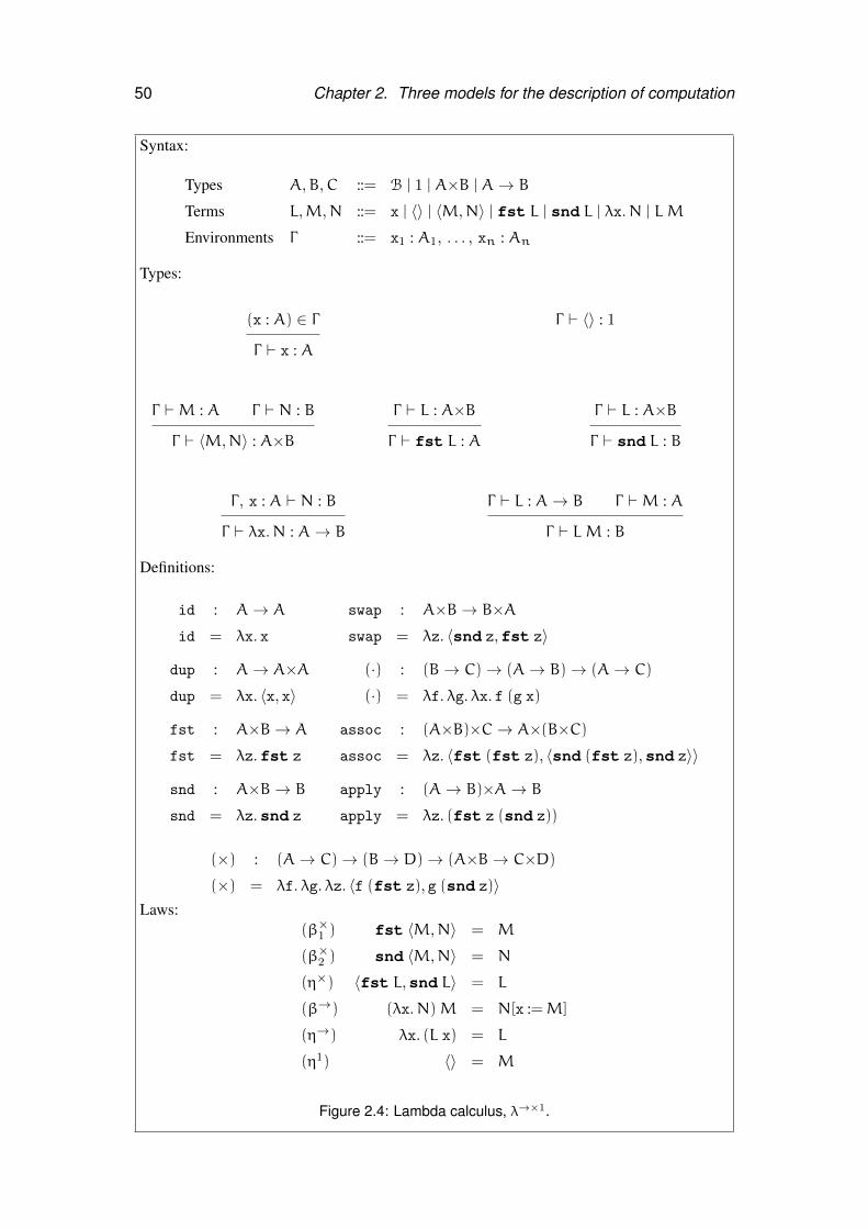
50 Chapter 2. Three models for the description of computation
Syntax:
Types A,B,C ::= B | 1 | A×B | A→ B
Terms L,M,N ::= x | 〈〉 | 〈M,N〉 | fst L | snd L | λx.N | L M
Environments Γ ::= x1 : A1, . . . , xn : An
Types:
(x : A) ∈ Γ
Γ ` x : A
Γ ` 〈〉 : 1
Γ `M : A Γ ` N : B
Γ ` 〈M,N〉 : A×B
Γ ` L : A×B
Γ ` fst L : A
Γ ` L : A×B
Γ ` snd L : B
Γ , x : A ` N : B
Γ ` λx.N : A→ B
Γ ` L : A→ B Γ `M : A
Γ ` L M : B
Definitions:
id : A→ A
id = λx. x
dup : A→ A×Adup = λx. 〈x, x〉
fst : A×B→ A
fst = λz.fst z
snd : A×B→ B
snd = λz.snd z
swap : A×B→ B×Aswap = λz. 〈snd z,fst z〉
(·) : (B→ C)→ (A→ B)→ (A→ C)
(·) = λf. λg. λx. f (g x)
assoc : (A×B)×C→ A×(B×C)assoc = λz. 〈fst (fst z), 〈snd (fst z),snd z〉〉
apply : (A→ B)×A→ B
apply = λz. (fst z (snd z))
(×) : (A→ C)→ (B→ D)→ (A×B→ C×D)
(×) = λf. λg. λz. 〈f (fst z), g (snd z)〉Laws:
(β×1 ) fst 〈M,N〉 = M
(β×2 ) snd 〈M,N〉 = N
(η×) 〈fst L,snd L〉 = L
(β→) (λx.N)M = N[x :=M]
(η→) λx. (L x) = L
(η1) 〈〉 = M
Figure 2.4: Lambda calculus, λ→×1.
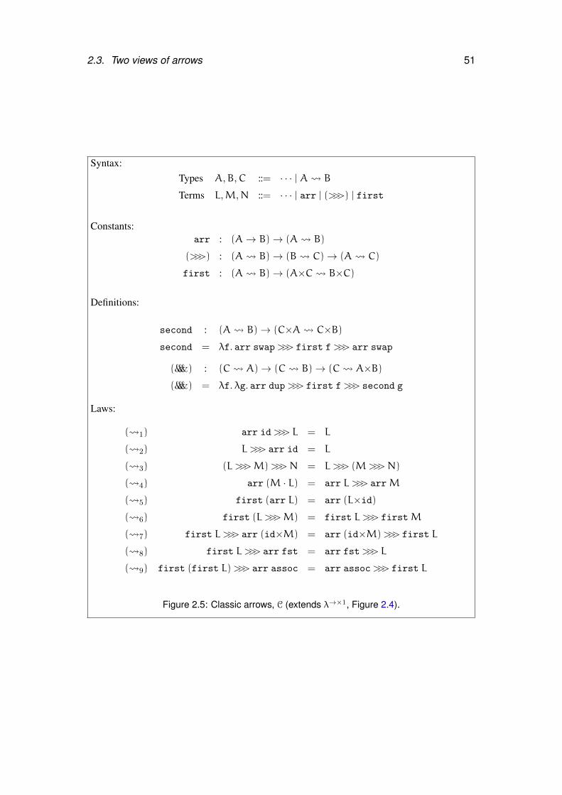
2.3. Two views of arrows 51
Syntax:Types A,B,C ::= · · · | A B
Terms L,M,N ::= · · · | arr | (>>>) | first
Constants:arr : (A→ B)→ (A B)
(>>>) : (A B)→ (B C)→ (A C)
first : (A B)→ (A×C B×C)
Definitions:
second : (A B)→ (C×A C×B)second = λf. arr swap>>> first f>>> arr swap
(&&&) : (C A)→ (C B)→ (C A×B)(&&&) = λf. λg. arr dup>>> first f>>> second g
Laws:
( 1) arr id>>> L = L
( 2) L >>> arr id = L
( 3) (L >>>M)>>>N = L >>> (M>>>N)
( 4) arr (M · L) = arr L >>> arrM
( 5) first (arr L) = arr (L×id)( 6) first (L >>>M) = first L >>> firstM
( 7) first L >>> arr (id×M) = arr (id×M)>>> first L
( 8) first L >>> arr fst = arr fst>>> L
( 9) first (first L)>>> arr assoc = arr assoc>>> first L
Figure 2.5: Classic arrows, C (extends λ→×1, Figure 2.4).
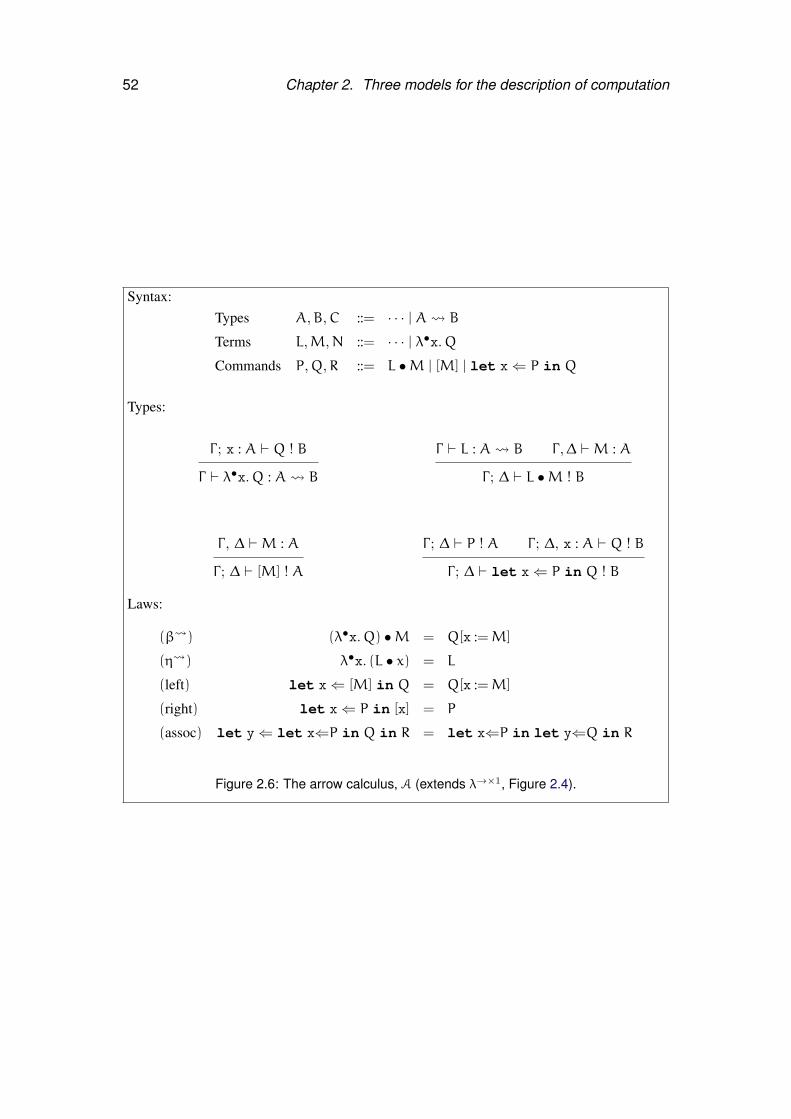
52 Chapter 2. Three models for the description of computation
Syntax:Types A,B,C ::= · · · | A B
Terms L,M,N ::= · · · | λ•x.Q
Commands P,Q,R ::= L •M | [M] | let x⇐ P in Q
Types:
Γ ; x : A ` Q ! B
Γ ` λ•x.Q : A B
Γ ` L : A B Γ ,∆ `M : A
Γ ; ∆ ` L •M ! B
Γ , ∆ `M : A
Γ ; ∆ ` [M] ! A
Γ ; ∆ ` P ! A Γ ; ∆, x : A ` Q ! B
Γ ; ∆ ` let x⇐ P in Q ! B
Laws:
(β ) (λ•x.Q) •M = Q[x :=M]
(η ) λ•x. (L • x) = L
(left) let x⇐ [M] in Q = Q[x :=M]
(right) let x⇐ P in [x] = P
(assoc) let y⇐ let x⇐P in Q in R = let x⇐P in let y⇐Q in R
Figure 2.6: The arrow calculus, A (extends λ→×1, Figure 2.4).
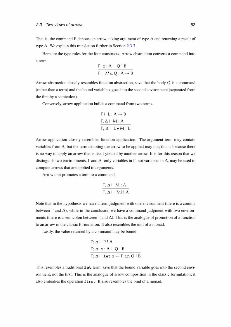
2.3. Two views of arrows 53
That is, the command P denotes an arrow, taking argument of type ∆ and returning a result of
type A. We explain this translation further in Section 2.3.3.
Here are the type rules for the four constructs. Arrow abstraction converts a command into
a term.Γ ; x : A ` Q ! B
Γ ` λ•x.Q : A B
Arrow abstraction closely resembles function abstraction, save that the body Q is a command
(rather than a term) and the bound variable x goes into the second environment (separated from
the first by a semicolon).
Conversely, arrow application builds a command from two terms.
Γ ` L : A B
Γ ,∆ `M : A
Γ ; ∆ ` L •M ! B
Arrow application closely resembles function application. The argument term may contain
variables from ∆, but the term denoting the arrow to be applied may not; this is because there
is no way to apply an arrow that is itself yielded by another arrow. It is for this reason that we
distinguish two environments, Γ and ∆: only variables in Γ , not variables in ∆, may be used to
compute arrows that are applied to arguments.
Arrow unit promotes a term to a command.
Γ , ∆ `M : A
Γ ; ∆ ` [M] ! A
Note that in the hypothesis we have a term judgment with one environment (there is a comma
between Γ and ∆), while in the conclusion we have a command judgment with two environ-
ments (there is a semicolon between Γ and ∆). This is the analogue of promotion of a function
to an arrow in the classic formulation. It also resembles the unit of a monad.
Lastly, the value returned by a command may be bound.
Γ ; ∆ ` P ! A
Γ ; ∆, x : A ` Q ! B
Γ ; ∆ ` let x⇐ P in Q ! B
This resembles a traditional let term, save that the bound variable goes into the second envi-
ronment, not the first. This is the analogue of arrow composition in the classic formulation; it
also embodies the operation first. It also resembles the bind of a monad.
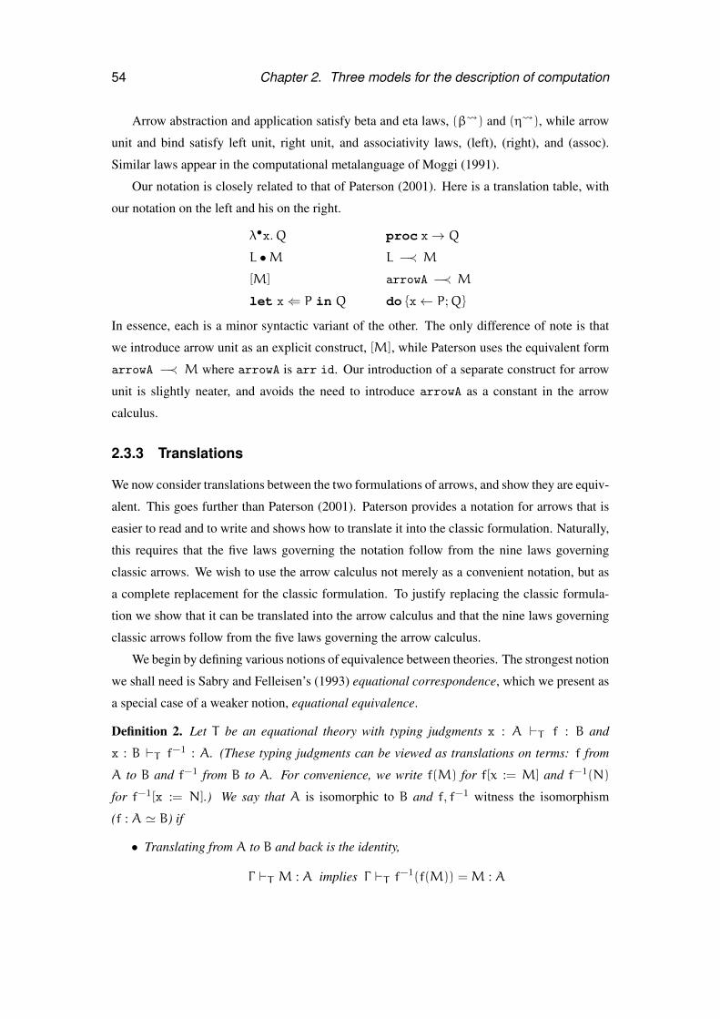
54 Chapter 2. Three models for the description of computation
Arrow abstraction and application satisfy beta and eta laws, (β ) and (η ), while arrow
unit and bind satisfy left unit, right unit, and associativity laws, (left), (right), and (assoc).
Similar laws appear in the computational metalanguage of Moggi (1991).
Our notation is closely related to that of Paterson (2001). Here is a translation table, with
our notation on the left and his on the right.
λ•x.Q proc x→ Q
L •M L −≺ M
[M] arrowA −≺ M
let x⇐ P in Q do {x← P;Q}
In essence, each is a minor syntactic variant of the other. The only difference of note is that
we introduce arrow unit as an explicit construct, [M], while Paterson uses the equivalent form
arrowA −≺ M where arrowA is arr id. Our introduction of a separate construct for arrow
unit is slightly neater, and avoids the need to introduce arrowA as a constant in the arrow
calculus.
2.3.3 Translations
We now consider translations between the two formulations of arrows, and show they are equiv-
alent. This goes further than Paterson (2001). Paterson provides a notation for arrows that is
easier to read and to write and shows how to translate it into the classic formulation. Naturally,
this requires that the five laws governing the notation follow from the nine laws governing
classic arrows. We wish to use the arrow calculus not merely as a convenient notation, but as
a complete replacement for the classic formulation. To justify replacing the classic formula-
tion we show that it can be translated into the arrow calculus and that the nine laws governing
classic arrows follow from the five laws governing the arrow calculus.
We begin by defining various notions of equivalence between theories. The strongest notion
we shall need is Sabry and Felleisen’s (1993) equational correspondence, which we present as
a special case of a weaker notion, equational equivalence.
Definition 2. Let T be an equational theory with typing judgments x : A `T f : B and
x : B `T f−1 : A. (These typing judgments can be viewed as translations on terms: f from
A to B and f−1 from B to A. For convenience, we write f(M) for f[x := M] and f−1(N)
for f−1[x := N].) We say that A is isomorphic to B and f, f−1 witness the isomorphism
(f : A ' B) if
• Translating from A to B and back is the identity,
Γ `T M : A implies Γ `T f−1(f(M)) =M : A
2.3. Two views of arrows 55
for all Γ ,M,A in T .
• Translating from B to A and back is the identity,
Γ `T N : B implies Γ `T f(f−1(N)) = N : B
for all Γ ,N,B in T .
As all of the theories we consider include function types and lambda abstractions, we
choose to express the isomorphisms more concisely as pairs of closed terms f : A → B and
f−1 : B→ A rather than typing judgments x : A `T f : B and x : B `T f−1 : A.
Definition 3. Let S, T be equational theories, with a translation on types and terms J−K from
S to T . We say that J−K preserves typing if
Γ `S M : A implies JΓK `T JMK : JAK
for all Γ ,M,A in S.
Definition 4. Let S, T be equational theories, with a translation on types and terms J−K from
S to T that preserves typing. We say that J−K is compositional if
Γ `S N : A and Γ , x : A `S M : B
implies
JΓK `T JM[x :=N]K = JMK[x := JNK] : JBK
for all Γ ,M,N,A,B in S.
Definition 5. Let S, T be equational theories, with a compositional translation on terms and
types J−K from S to T that preserves typing, and with a compositional inverse translation 〈[−]〉from T to S that also preserves typing. Further, translating a type from S to T and back yields
a type isomorphic to the original type,
fA : A ' 〈[JAK]〉
for all A in S. Similarly, translating a type from T to S and back yields a type isomorphic to
the original type,
gA : A ' J〈[A]〉K
for all A in T . We say these translations form an equational equivalence (S ∼ T ) if
56 Chapter 2. Three models for the description of computation
• The translation from S to T preserves equations,
Γ `S M = N : A implies JΓK `T JMK = JNK : JAK
for all Γ ,M,N,A in S.
• The translation from T to S preserves equations,
Γ `T M = N : A implies 〈[Γ ]〉 `S 〈[M]〉 = 〈[N]〉 : 〈[A]〉
for all Γ ,M,N,A in T .
• Translating from S to T and back yields a term isomorphic to the original term,
Γ `S M : A implies Γ `S 〈[JMK]〉[Γ := f(Γ)] = fA(M) : 〈[JAK]〉
for all Γ ,M,A in S (writing N[Γ := f(Γ)] for N[x1 := fA1(x1), . . . , xn := fAn(xn)],
given Γ = x1 : A1, . . . , xn : An).
• Translating from T to S and back yields a term isomorphic to the original term,
Γ `T M : A implies Γ `T J〈[M]〉K[Γ := g(Γ)] = gA(M) : J〈[A]〉K
for all Γ ,M,A in T .
(This definition is analogous to saying that we have an equivalence of categories (Mac Lane,
1998), where J−K is left adjoint to 〈[−]〉 with unit fA and counit g−1A .)
The special case of an equational equivalence where both isomorphisms are the identity is
an equational correspondence.
Definition 6. An equational correspondence between theories S and T (S ∼= T ) is an equa-
tional equivalence with translations J−K : S → T , 〈[−]〉 : T → S where both fA and gAare the identity at each type A. (This is analogous to saying that we have an isomorphism of
categories (Mac Lane, 1998) given by the translations J−K : S→ T and 〈[−]〉 : T → S.)
We also introduce the notion of equational embedding, a map from a weaker into a stronger
theory. An equational embedding of a theory S into a theory T may be defined as an equational
equivalence between S and a subtheory of T . We instead use the following more direct defini-
tion, which is more convenient in practice.
Definition 7. Let S, T be equational theories with a compositional translation on terms and
types J−K from S to T that preserves typing, and with a compositional inverse translation 〈[−]〉from the image of J−K (written JSK) to S that also preserves typing,
JΓK `T JMK : JAK implies 〈[JΓK]〉 `S 〈[JMK]〉 : 〈[JAK]〉
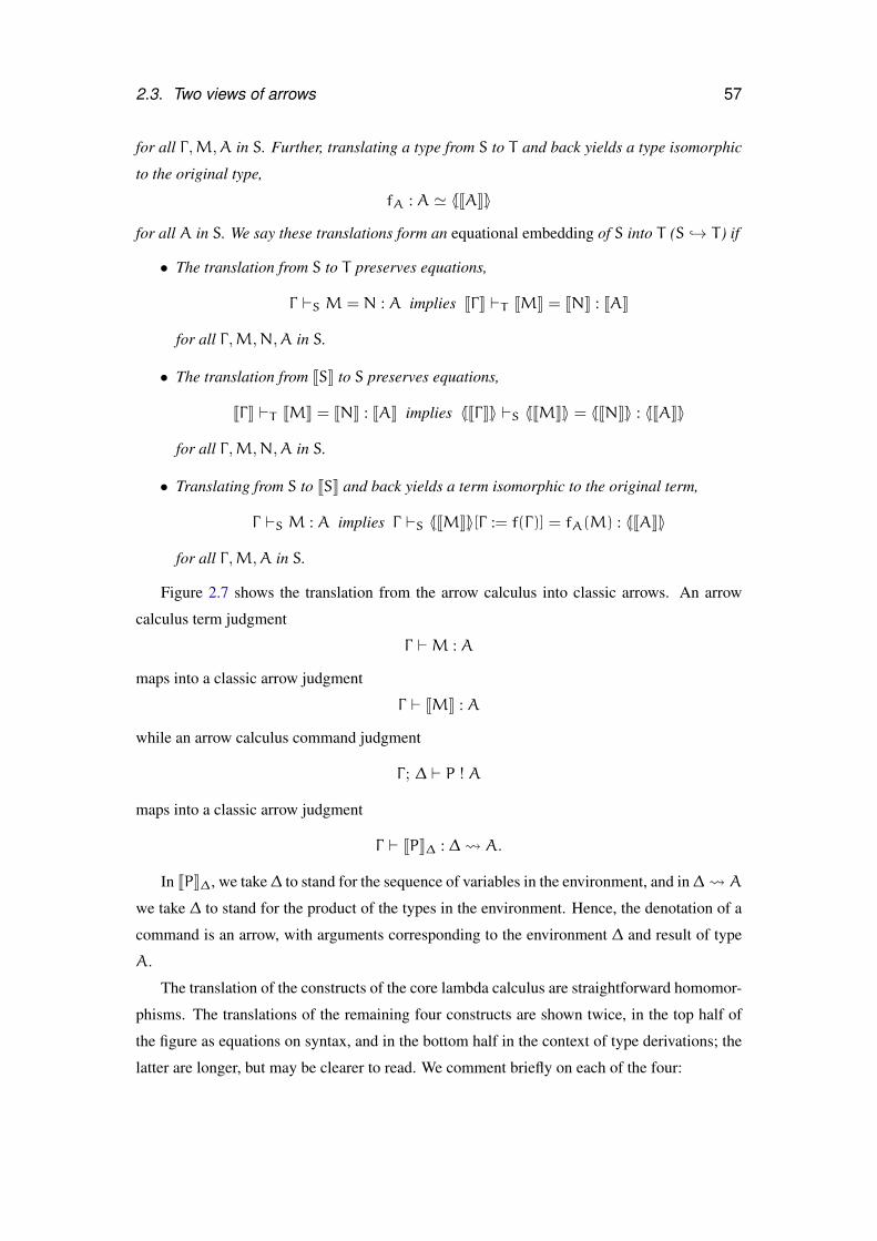
2.3. Two views of arrows 57
for all Γ ,M,A in S. Further, translating a type from S to T and back yields a type isomorphic
to the original type,
fA : A ' 〈[JAK]〉
for all A in S. We say these translations form an equational embedding of S into T (S ↪→ T ) if
• The translation from S to T preserves equations,
Γ `S M = N : A implies JΓK `T JMK = JNK : JAK
for all Γ ,M,N,A in S.
• The translation from JSK to S preserves equations,
JΓK `T JMK = JNK : JAK implies 〈[JΓK]〉 `S 〈[JMK]〉 = 〈[JNK]〉 : 〈[JAK]〉
for all Γ ,M,N,A in S.
• Translating from S to JSK and back yields a term isomorphic to the original term,
Γ `S M : A implies Γ `S 〈[JMK]〉[Γ := f(Γ)] = fA(M) : 〈[JAK]〉
for all Γ ,M,A in S.
Figure 2.7 shows the translation from the arrow calculus into classic arrows. An arrow
calculus term judgment
Γ `M : A
maps into a classic arrow judgment
Γ ` JMK : A
while an arrow calculus command judgment
Γ ; ∆ ` P ! A
maps into a classic arrow judgment
Γ ` JPK∆ : ∆ A.
In JPK∆, we take∆ to stand for the sequence of variables in the environment, and in∆ A
we take ∆ to stand for the product of the types in the environment. Hence, the denotation of a
command is an arrow, with arguments corresponding to the environment ∆ and result of type
A.
The translation of the constructs of the core lambda calculus are straightforward homomor-
phisms. The translations of the remaining four constructs are shown twice, in the top half of
the figure as equations on syntax, and in the bottom half in the context of type derivations; the
latter are longer, but may be clearer to read. We comment briefly on each of the four:
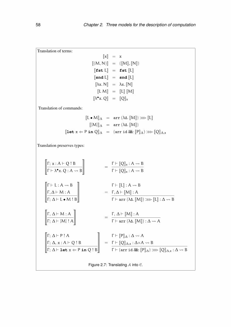
58 Chapter 2. Three models for the description of computation
Translation of terms:JxK = x
J(M,N)K = (JMK, JNK)
Jfst LK = fst JLK
Jsnd LK = snd JLK
Jλx.NK = λx. JNK
JL MK = JLK JMK
Jλ•x.QK = JQKx
Translation of commands:
JL •MK∆ = arr (λ∆. JMK)>>> JLK
J[M]K∆ = arr (λ∆. JMK)
Jlet x⇐ P in QK∆ = (arr id &&& JPK∆)>>> JQK∆,x
Translation preserves types:
u
vΓ ; x : A ` Q ! B
Γ ` λ•x.Q : A B
}
~ =Γ ` JQKx : A B
Γ ` JQKx : A B
u
wwv
Γ ` L : A B
Γ ,∆ `M : A
Γ ; ∆ ` L •M ! B
}
��~ =
Γ ` JLK : A B
Γ ,∆ ` JMK : A
Γ ` arr (λ∆. JMK)>>> JLK : ∆ B
u
vΓ , ∆ `M : A
Γ ; ∆ ` [M] ! A
}
~ =Γ , ∆ ` JMK : A
Γ ` arr (λ∆. JMK) : ∆ A
u
wwv
Γ ; ∆ ` P ! A
Γ ; ∆, x : A ` Q ! B
Γ ; ∆ ` let x⇐ P in Q ! B
}
��~ =
Γ ` JPK∆ : ∆ A
Γ ` JQK∆,x : ∆×A B
Γ ` (arr id &&& JPK∆)>>> JQK∆,x : ∆ B
Figure 2.7: Translating A into C.
2.3. Two views of arrows 59
Translation:
〈[x]〉 = x
〈[(M,N)]〉 = (〈[M]〉, 〈[N]〉)〈[fst L]〉 = fst 〈[L]〉〈[snd L]〉 = snd 〈[L]〉〈[λx.N]〉 = λx. 〈[N]〉〈[L M]〉 = 〈[L]〉 〈[M]〉〈[arr]〉 = λf. λ•x. [f x]
〈[(>>>)]〉 = λf. λg. λ•x.let y⇐ (f • x) in g • y〈[first]〉 = λf. λ•z.let x⇐ f • fst z in [〈x,snd z〉]
Figure 2.8: Translating C into A.
• λ•x.N translates straightforwardly; it is a no-op.
• L •M translates to >>>.
• [M] translates to arr.
• let x ⇐ P in Q translates to pairing &&& (to extend the environment with P) and
composition >>> (to then apply Q).
The translation uses the notation λ∆.N, which is given the obvious meaning: λx.N stands for
itself, and λx1, x2.N stands for λz.N[x1 :=fst z, x2 :=snd z], and λx1, x2, x3.N stands for
λz.N[x1 :=fst (fst z), x2 :=snd (fst z), x3 :=snd z], and so on. (This definition assumes
a non-empty environment, and in fact ∆ is always non-empty in this translation. However, it is
not always non-empty in the related translations in Section 2.4. It is straightforward to adjust
the definitions here to support the empty-environment case: for example, we might take the
empty environment · to stand for the unit type when used as a type, and take λx1, x2.N to
stand for λz.N[x1 := snd (fst z), x2 := snd z], and so on. A second possibility is to define
the translation differently for empty and non-empty environments, retaining the translation we
have given for the case where the environment is non-empty. A third possibility is to ensure via
weakening (which we will define in Lemma 9) that the environment is never actually empty.
Rather than obscure the presentation with these details we will retain our existing definitions,
on the understanding that they can be easily adjusted to support the empty-environment case
where necessary.)
60 Chapter 2. Three models for the description of computation
The inverse translation, from classic arrows to the arrow calculus, is given in Figure 2.8.
Again, the translation of the constructs of the core lambda calculus are straightforward homo-
morphisms. Each of the three constants translates to an appropriate term in the arrow calculus.
Demonstrating the equivalence of the two formulations of arrows requires that we translate
the laws. In order to translate the (β ) and (left) laws we must determine the meaning of
translation on a substitution, which we do with the following lemma.
Lemma 8. [Translating substitution from A to C]
The translations of substitution on terms and commands from A to C satisfy the following
equations.
JM[x :=N]K = JMK[x := JNK]
JP[x :=N]K∆ = arr (λ∆.(∆, JNK))>>> JPK∆,x
Proof. By mutual induction on the derivations of P and M. There is one case for each term
form and each command form. Appendix A.2 gives the full proof.
Now consider the translation of the (assoc) law. The left side translates as follows:
Jlet y⇐ (let x⇐ P in Q) in RK∆= (arr id &&& ((arr id &&& JPK∆)>>> JQK∆,x))>>> JRK∆,x
and the right side translates as follows:
Jlet x⇐ P in (let y⇐ Q in R)K∆= (arr id &&& JPK∆)>>> ((arr id &&& JQK∆,x)>>> JRK∆,x,y)
Notice that the left side contains the term JRK∆,x — the translation of the command R in the
environment ∆, x — while the right side contains the term JRK∆,x,y — the translation of R in
the environment ∆, x, y. The following two lemmas define weakening in the arrow calculus
and its effects of the translation, allowing us to establish the equivalence of the two sides.
Lemma 9 (Weakening). Suppose type environments Γ , ∆, Γ ′, ∆ ′, such that Γ ⊆ Γ ′ and Γ ,∆ ⊆Γ ′,∆ ′. Then if
Γ `M : A
is derivable for some type A then
Γ ′ `M : A
is also derivable, and if
Γ ; ∆ ` P ! B
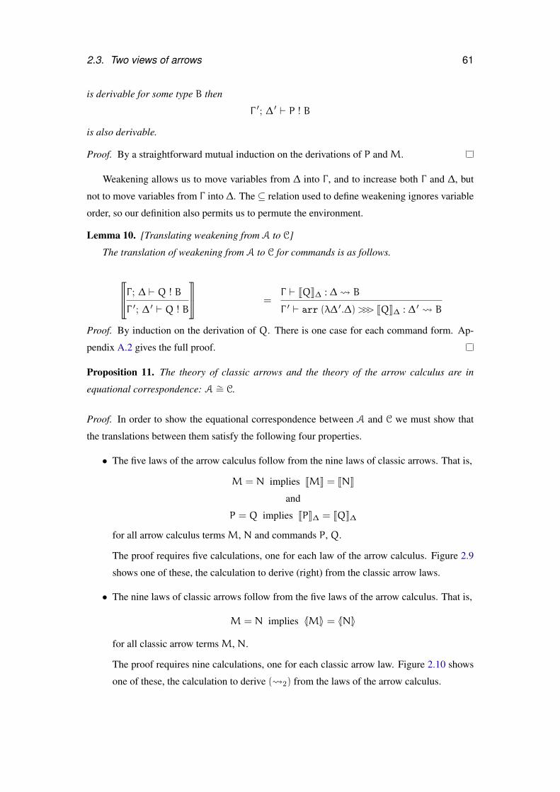
2.3. Two views of arrows 61
is derivable for some type B then
Γ ′; ∆ ′ ` P ! B
is also derivable.
Proof. By a straightforward mutual induction on the derivations of P andM.
Weakening allows us to move variables from ∆ into Γ , and to increase both Γ and ∆, but
not to move variables from Γ into ∆. The ⊆ relation used to define weakening ignores variable
order, so our definition also permits us to permute the environment.
Lemma 10. [Translating weakening from A to C]
The translation of weakening from A to C for commands is as follows.
u
vΓ ; ∆ ` Q ! B
Γ ′; ∆ ′ ` Q ! B
}
~ =Γ ` JQK∆ : ∆ B
Γ ′ ` arr (λ∆ ′.∆)>>> JQK∆ : ∆ ′ B
Proof. By induction on the derivation of Q. There is one case for each command form. Ap-
pendix A.2 gives the full proof.
Proposition 11. The theory of classic arrows and the theory of the arrow calculus are in
equational correspondence: A ∼= C.
Proof. In order to show the equational correspondence between A and C we must show that
the translations between them satisfy the following four properties.
• The five laws of the arrow calculus follow from the nine laws of classic arrows. That is,
M = N implies JMK = JNK
and
P = Q implies JPK∆ = JQK∆
for all arrow calculus termsM, N and commands P, Q.
The proof requires five calculations, one for each law of the arrow calculus. Figure 2.9
shows one of these, the calculation to derive (right) from the classic arrow laws.
• The nine laws of classic arrows follow from the five laws of the arrow calculus. That is,
M = N implies 〈[M]〉 = 〈[N]〉
for all classic arrow termsM, N.
The proof requires nine calculations, one for each classic arrow law. Figure 2.10 shows
one of these, the calculation to derive ( 2) from the laws of the arrow calculus.
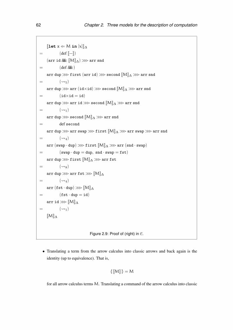
62 Chapter 2. Three models for the description of computation
Jlet x⇐M in [x]K∆= (def J−K)
(arr id &&& JMK∆)>>> arr snd
= (def &&&)
arr dup>>> first (arr id)>>> second JMK∆ >>> arr snd
= ( 5)
arr dup>>> arr (id×id)>>> second JMK∆ >>> arr snd
= (id×id = id)
arr dup>>> arr id>>> second JMK∆ >>> arr snd
= ( 1)
arr dup>>> second JMK∆ >>> arr snd
= def second
arr dup>>> arr swap>>> first JMK∆ >>> arr swap>>> arr snd
= ( 4)
arr (swap · dup)>>> first JMK∆ >>> arr (snd · swap)= (swap · dup = dup, snd · swap = fst)
arr dup>>> first JMK∆ >>> arr fst
= ( 8)
arr dup>>> arr fst>>> JMK∆= ( 4)
arr (fst · dup)>>> JMK∆= (fst · dup = id)
arr id>>> JMK∆= ( 1)
JMK∆
Figure 2.9: Proof of (right) in C.
• Translating a term from the arrow calculus into classic arrows and back again is the
identity (up to equivalence). That is,
〈[ JMK ]〉 =M
for all arrow calculus termsM. Translating a command of the arrow calculus into classic
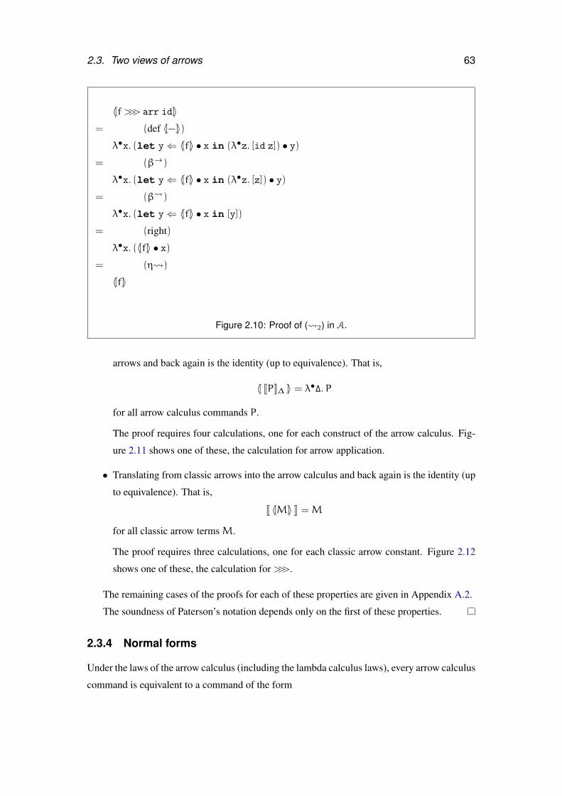
2.3. Two views of arrows 63
〈[f >>> arr id]〉= (def 〈[−]〉)
λ•x. (let y⇐ 〈[f]〉 • x in (λ•z. [id z]) • y)= (β→)
λ•x. (let y⇐ 〈[f]〉 • x in (λ•z. [z]) • y)= (β )
λ•x. (let y⇐ 〈[f]〉 • x in [y])
= (right)
λ•x. (〈[f]〉 • x)= (η )
〈[f]〉
Figure 2.10: Proof of ( 2) in A.
arrows and back again is the identity (up to equivalence). That is,
〈[ JPK∆ ]〉 = λ•∆.P
for all arrow calculus commands P.
The proof requires four calculations, one for each construct of the arrow calculus. Fig-
ure 2.11 shows one of these, the calculation for arrow application.
• Translating from classic arrows into the arrow calculus and back again is the identity (up
to equivalence). That is,
J 〈[M]〉 K =M
for all classic arrow termsM.
The proof requires three calculations, one for each classic arrow constant. Figure 2.12
shows one of these, the calculation for >>>.
The remaining cases of the proofs for each of these properties are given in Appendix A.2.
The soundness of Paterson’s notation depends only on the first of these properties.
2.3.4 Normal forms
Under the laws of the arrow calculus (including the lambda calculus laws), every arrow calculus
command is equivalent to a command of the form
64 Chapter 2. Three models for the description of computation
〈[ JL •MK∆ ]〉 • ∆= (def J−K∆)
〈[ arr (λ∆. JMK)>>> JLK ]〉 • ∆= (def 〈[−]〉)
λ•∆. (let y⇐ (λ•z. [(λ∆. 〈[JMK]〉) z]) • ∆ in 〈[JLK]〉 • y) • ∆= (induction hypothesis)
λ•∆. (let y⇐ (λ•z. [(λ∆.M) z]) • ∆ in L • y) • ∆= (β )
let y⇐ [(λ∆.M) ∆] in L • y= (β→)
let y⇐ [M] in L • y= (left)
L •M
Figure 2.11: Translating L •M to C and back.
let x1 ⇐ c1 • M1 in. . .let xn ⇐ cn • Mn in[N]
where c1, . . . , cn are constants of arrow type and M1, . . . ,Mn,N are in normal form. There
is a connection to the normal form for classic arrows given in Section 2.2.5.1: the result of
translating an arrow calculus command in normal form is a classic arrow term in normal form,
except for the order of the operands to &&& (which is a matter of mere convenience).
The technical report on arrows (Lindley et al., 2008a) explains how to obtain a rewriting
theory for arrow calculus from the equational theory by orienting the rules appropriately. Proofs
of confluence and strong normalisation follow from a translation of arrow calculus into Moggi’s
metalanguage for monads, which is known to be strongly normalising (Lindley and Stark,
2005).
2.3.5 Redundancy of the second law
In Section 2.2.5.1 we saw that classic arrow terms can be normalised using eight of the nine
laws: the right unit law ( 2) is not needed. The proof of the equational correspondence
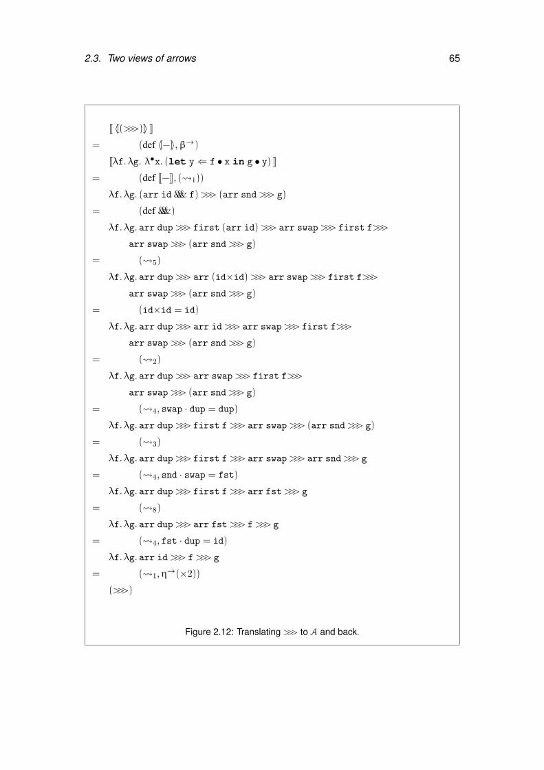
2.3. Two views of arrows 65
J 〈[(>>>)]〉 K= (def 〈[−]〉,β→)
Jλf. λg. λ•x. (let y⇐ f • x in g • y) K= (def J−K, ( 1))
λf. λg. (arr id &&& f)>>> (arr snd>>> g)
= (def &&&)
λf. λg. arr dup>>> first (arr id)>>> arr swap>>> first f>>>
arr swap>>> (arr snd>>> g)
= ( 5)
λf. λg. arr dup>>> arr (id×id)>>> arr swap>>> first f>>>
arr swap>>> (arr snd>>> g)
= (id×id = id)
λf. λg. arr dup>>> arr id>>> arr swap>>> first f>>>
arr swap>>> (arr snd>>> g)
= ( 2)
λf. λg. arr dup>>> arr swap>>> first f>>>
arr swap>>> (arr snd>>> g)
= ( 4, swap · dup = dup)
λf. λg. arr dup>>> first f>>> arr swap>>> (arr snd>>> g)
= ( 3)
λf. λg. arr dup>>> first f>>> arr swap>>> arr snd>>> g
= ( 4, snd · swap = fst)
λf. λg. arr dup>>> first f>>> arr fst>>> g
= ( 8)
λf. λg. arr dup>>> arr fst>>> f>>> g
= ( 4, fst · dup = id)
λf. λg. arr id>>> f>>> g
= ( 1,η→(×2))
(>>>)
Figure 2.12: Translating >>> to A and back.
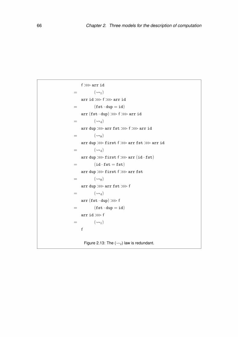
66 Chapter 2. Three models for the description of computation
f >>> arr id
= ( 1)
arr id>>> f >>> arr id
= (fst · dup = id)
arr (fst · dup)>>> f >>> arr id
= ( 4)
arr dup>>> arr fst>>> f >>> arr id
= ( 8)
arr dup>>> first f >>> arr fst>>> arr id
= ( 4)
arr dup>>> first f >>> arr (id · fst)= (id · fst = fst)
arr dup>>> first f >>> arr fst
= ( 8)
arr dup>>> arr fst>>> f
= ( 4)
arr (fst · dup)>>> f= (fst · dup = id)
arr id>>> f
= ( 1)
f
Figure 2.13: The ( 2) law is redundant.
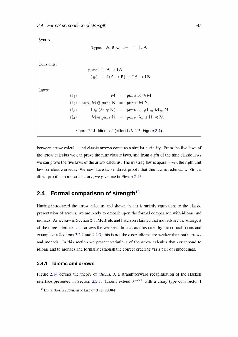
2.4. Formal comparison of strength 67
Syntax:
Types A,B,C ::= · · · | IA
Constants:pure : A→ IA
(�) : I (A→ B)→ IA→ I B
Laws:(I1) M = pure id�M
(I2) pureM� pure N = pure (MN)
(I3) L� (M�N) = pure (·)� L�M�N
(I4) M� pure N = pure (λf. f N)�M
Figure 2.14: Idioms, I (extends λ→×1, Figure 2.4).
between arrow calculus and classic arrows contains a similar curiosity. From the five laws of
the arrow calculus we can prove the nine classic laws, and from eight of the nine classic laws
we can prove the five laws of the arrow calculus. The missing law is again ( 2), the right unit
law for classic arrows. We now have two indirect proofs that this law is redundant. Still, a
direct proof is more satisfactory; we give one in Figure 2.13.
2.4 Formal comparison of strength10
Having introduced the arrow calculus and shown that it is strictly equivalent to the classic
presentation of arrows, we are ready to embark upon the formal comparison with idioms and
monads. As we saw in Section 2.3, McBride and Paterson claimed that monads are the strongest
of the three interfaces and arrows the weakest. In fact, as illustrated by the normal forms and
examples in Sections 2.2.2 and 2.2.3, this is not the case: idioms are weaker than both arrows
and monads. In this section we present variations of the arrow calculus that correspond to
idioms and to monads and formally establish the correct ordering via a pair of embeddings.
2.4.1 Idioms and arrows
Figure 2.14 defines the theory of idioms, I, a straightforward recapitulation of the Haskell
interface presented in Section 2.2.3. Idioms extend λ→×1 with a unary type constructor I
10This section is a revision of Lindley et al. (2008b)
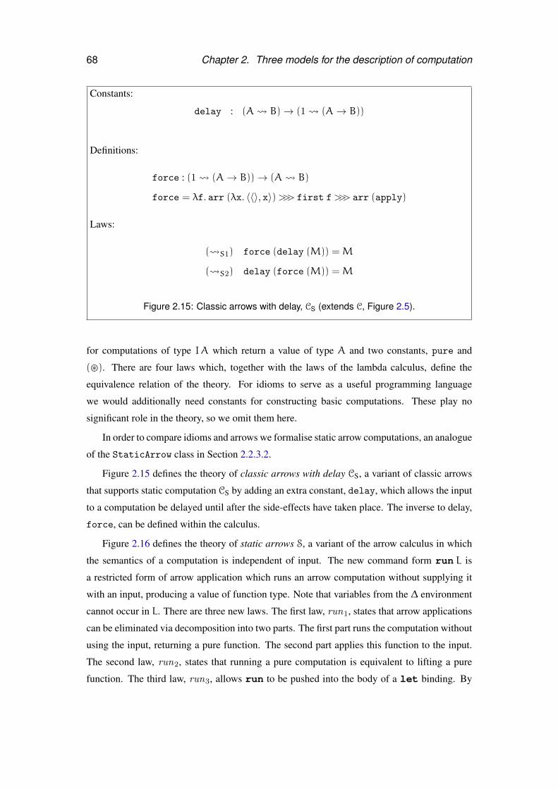
68 Chapter 2. Three models for the description of computation
Constants:
delay : (A B)→ (1 (A→ B))
Definitions:
force : (1 (A→ B))→ (A B)
force = λf. arr (λx. 〈〈〉, x〉)>>> first f>>> arr (apply)
Laws:
( S1) force (delay (M)) =M
( S2) delay (force (M)) =M
Figure 2.15: Classic arrows with delay, CS (extends C, Figure 2.5).
for computations of type IA which return a value of type A and two constants, pure and
(�). There are four laws which, together with the laws of the lambda calculus, define the
equivalence relation of the theory. For idioms to serve as a useful programming language
we would additionally need constants for constructing basic computations. These play no
significant role in the theory, so we omit them here.
In order to compare idioms and arrows we formalise static arrow computations, an analogue
of the StaticArrow class in Section 2.2.3.2.
Figure 2.15 defines the theory of classic arrows with delay CS, a variant of classic arrows
that supports static computation CS by adding an extra constant, delay, which allows the input
to a computation be delayed until after the side-effects have taken place. The inverse to delay,
force, can be defined within the calculus.
Figure 2.16 defines the theory of static arrows S, a variant of the arrow calculus in which
the semantics of a computation is independent of input. The new command form run L is
a restricted form of arrow application which runs an arrow computation without supplying it
with an input, producing a value of function type. Note that variables from the ∆ environment
cannot occur in L. There are three new laws. The first law, run1, states that arrow applications
can be eliminated via decomposition into two parts. The first part runs the computation without
using the input, returning a pure function. The second part applies this function to the input.
The second law, run2, states that running a pure computation is equivalent to lifting a pure
function. The third law, run3, allows run to be pushed into the body of a let binding. By
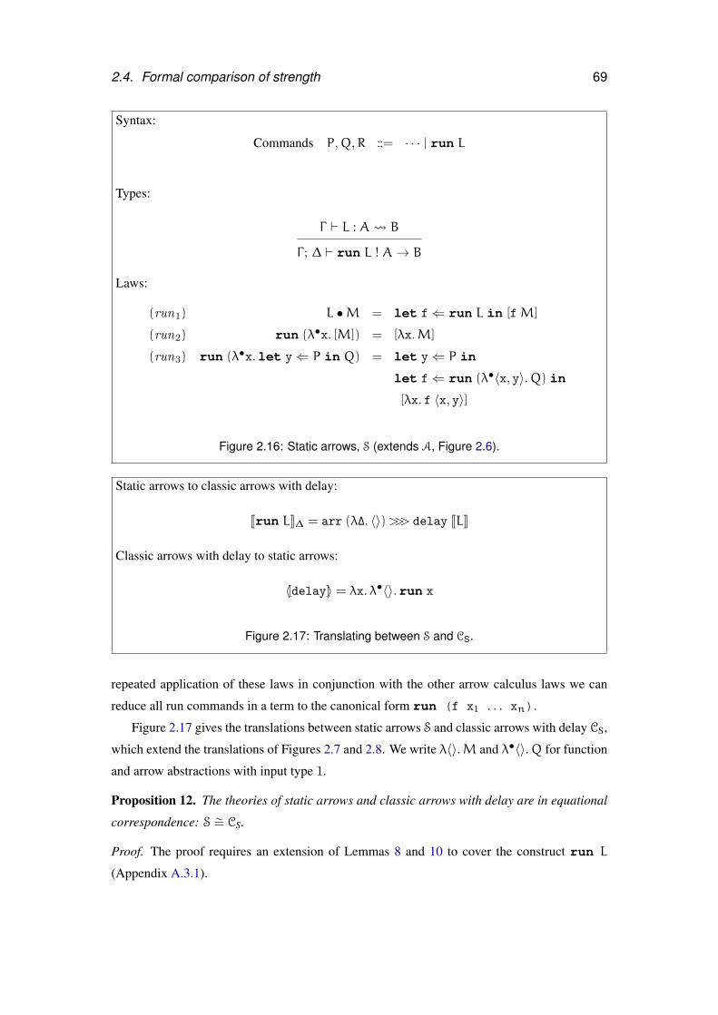
2.4. Formal comparison of strength 69
Syntax:
Commands P,Q,R ::= · · · | run L
Types:
Γ ` L : A B
Γ ; ∆ ` run L ! A→ B
Laws:
(run1) L •M = let f⇐ run L in [fM]
(run2) run (λ•x. [M]) = [λx.M]
(run3) run (λ•x.let y⇐ P in Q) = let y⇐ P in
let f⇐ run (λ•〈x, y〉.Q) in
[λx. f 〈x, y〉]
Figure 2.16: Static arrows, S (extends A, Figure 2.6).
Static arrows to classic arrows with delay:
Jrun LK∆ = arr (λ∆. 〈〉)>>> delay JLK
Classic arrows with delay to static arrows:
〈[delay]〉 = λx. λ•〈〉.run x
Figure 2.17: Translating between S and CS.
repeated application of these laws in conjunction with the other arrow calculus laws we can
reduce all run commands in a term to the canonical form run (f x1 . . . xn).
Figure 2.17 gives the translations between static arrows S and classic arrows with delay CS,
which extend the translations of Figures 2.7 and 2.8. We write λ〈〉.M and λ•〈〉.Q for function
and arrow abstractions with input type 1.
Proposition 12. The theories of static arrows and classic arrows with delay are in equational
correspondence: S ∼= CS.
Proof. The proof requires an extension of Lemmas 8 and 10 to cover the construct run L
(Appendix A.3.1).
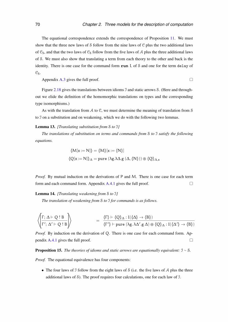
70 Chapter 2. Three models for the description of computation
The equational correspondence extends the correspondence of Proposition 11. We must
show that the three new laws of S follow from the nine laws of C plus the two additional laws
of CS, and that the two laws of CS follow from the five laws of A plus the three additional laws
of S. We must also show that translating a term from each theory to the other and back is the
identity. There is one case for the command form run L of S and one for the term delay of
CS.
Appendix A.3 gives the full proof.
Figure 2.18 gives the translations between idioms I and static arrows S. (Here and through-
out we elide the definition of the homomorphic translations on types and the corresponding
type isomorphisms.)
As with the translation from A to C, we must determine the meaning of translation from S
to I on a substitution and on weakening, which we do with the following two lemmas.
Lemma 13. [Translating substitution from S to I]
The translations of substitution on terms and commands from S to I satisfy the following
equations.
〈[M[x :=N]]〉 = 〈[M]〉[x := 〈[N]〉]
〈[Q[x :=N]]〉∆ = pure (λg.λ∆.g (∆, 〈[N]〉))� 〈[Q]〉∆,x
Proof. By mutual induction on the derivations of P and M. There is one case for each term
form and each command form. Appendix A.4.1 gives the full proof.
Lemma 14. [Translating weakening from S to I]
The translation of weakening from S to I for commands is as follows.
⟨Γ ; ∆ ` Q ! B
Γ ′; ∆ ′ ` Q ! B
⟩ =〈[Γ ]〉 ` 〈[Q]〉∆ : I(〈[∆]〉 → 〈[B]〉)〈[Γ ′]〉 ` pure (λg. λ∆ ′.g ∆)� 〈[Q]〉∆ : I(〈[∆ ′]〉 → 〈[B]〉)
Proof. By induction on the derivation of Q. There is one case for each command form. Ap-
pendix A.4.1 gives the full proof.
Proposition 15. The theories of idioms and static arrows are equationally equivalent: I ∼ S.
Proof. The equational equivalence has four components:
• The four laws of I follow from the eight laws of S (i.e. the five laws of A plus the three
additional laws of S). The proof requires four calculations, one for each law of I.
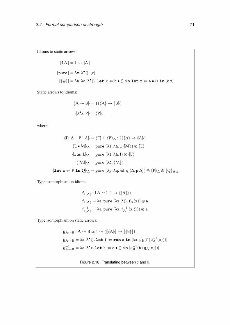
2.4. Formal comparison of strength 71
Idioms to static arrows:
JIAK = 1 JAK
JpureK = λx. λ•〈〉. [x]
J(�)K = λh. λa. λ•〈〉.let k⇐ h • 〈〉 in let x⇐ a • 〈〉 in [k x]
Static arrows to idioms:
〈[A B]〉 = I (〈[A]〉 → 〈[B]〉)
〈[λ•x.P]〉 = 〈[P]〉x
where
〈[Γ ; ∆ ` P ! A]〉 = 〈[Γ ]〉 ` 〈[P]〉∆ : I (〈[∆]〉 → 〈[A]〉)
〈[L •M]〉∆ = pure (λl. λ∆. l 〈[M]〉)� 〈[L]〉
〈[run L]〉∆ = pure (λl. λ∆. l)� 〈[L]〉
〈[[M]]〉∆ = pure (λ∆. 〈[M]〉)
〈[let x⇐ P in Q]〉∆ = pure (λp. λq. λ∆. q 〈∆, p ∆〉)� 〈[P]〉∆ � 〈[Q]〉∆,x
Type isomorphism on idioms:
fI(A) : IA ' I (1→ 〈[JAK]〉)
fI(A) = λa. pure (λx. λ〈〉. fA(x))� a
f−1I(A) = λa. pure (λx. f−1
A (x 〈〉))� a
Type isomorphism on static arrows:
gA B : A B ' 1 (J〈[A]〉K→ J〈[B]〉K)
gA B = λa. λ•〈〉.let f⇐ run a in [λx.gB(f (g−1A (x)))]
g−1A B = λa. λ•x.let h⇐ a • 〈〉 in [g−1
B (h (gA(x)))]
Figure 2.18: Translating between I and S.
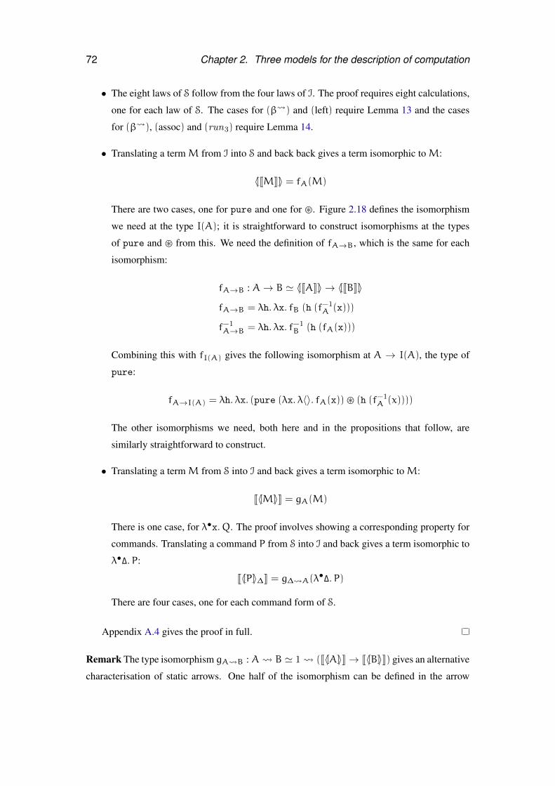
72 Chapter 2. Three models for the description of computation
• The eight laws of S follow from the four laws of I. The proof requires eight calculations,
one for each law of S. The cases for (β ) and (left) require Lemma 13 and the cases
for (β ), (assoc) and (run3) require Lemma 14.
• Translating a termM from I into S and back back gives a term isomorphic toM:
〈[JMK]〉 = fA(M)
There are two cases, one for pure and one for �. Figure 2.18 defines the isomorphism
we need at the type I(A); it is straightforward to construct isomorphisms at the types
of pure and � from this. We need the definition of fA→B, which is the same for each
isomorphism:
fA→B : A→ B ' 〈[JAK]〉 → 〈[JBK]〉
fA→B = λh. λx. fB (h (f−1A (x)))
f−1A→B = λh. λx. f−1
B (h (fA(x)))
Combining this with fI(A) gives the following isomorphism at A → I(A), the type of
pure:
fA→I(A) = λh. λx. (pure (λx. λ〈〉. fA(x))� (h (f−1A (x))))
The other isomorphisms we need, both here and in the propositions that follow, are
similarly straightforward to construct.
• Translating a termM from S into I and back gives a term isomorphic toM:
J〈[M]〉K = gA(M)
There is one case, for λ•x.Q. The proof involves showing a corresponding property for
commands. Translating a command P from S into I and back gives a term isomorphic to
λ•∆.P:
J〈[P]〉∆K = g∆ A(λ•∆.P)
There are four cases, one for each command form of S.
Appendix A.4 gives the proof in full.
Remark The type isomorphism gA B : A B ' 1 (J〈[A]〉K→ J〈[B]〉K) gives an alternative
characterisation of static arrows. One half of the isomorphism can be defined in the arrow
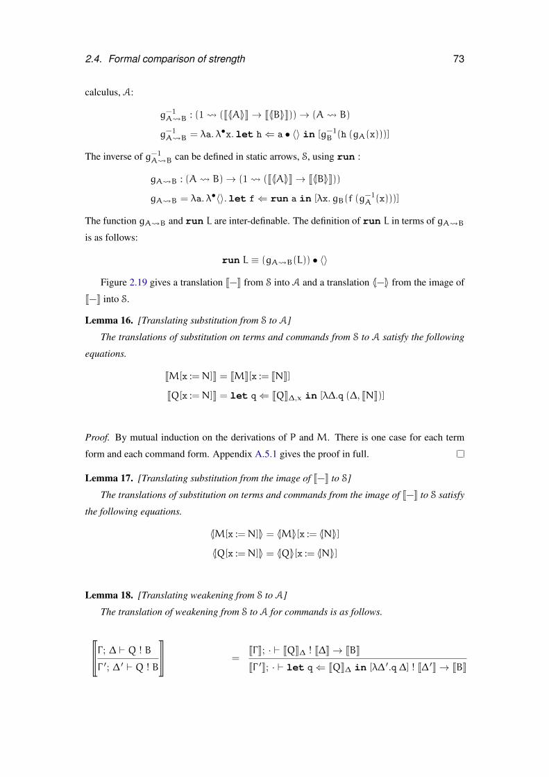
2.4. Formal comparison of strength 73
calculus, A:
g−1A B : (1 (J〈[A]〉K→ J〈[B]〉K))→ (A B)
g−1A B = λa. λ•x.let h⇐ a • 〈〉 in [g−1
B (h (gA(x)))]
The inverse of g−1A B can be defined in static arrows, S, using run :
gA B : (A B)→ (1 (J〈[A]〉K→ J〈[B]〉K))
gA B = λa. λ•〈〉.let f⇐ run a in [λx.gB(f (g−1A (x)))]
The function gA B and run L are inter-definable. The definition of run L in terms of gA Bis as follows:
run L ≡ (gA B(L)) • 〈〉
Figure 2.19 gives a translation J−K from S into A and a translation 〈[−]〉 from the image of
J−K into S.
Lemma 16. [Translating substitution from S to A]
The translations of substitution on terms and commands from S to A satisfy the following
equations.
JM[x :=N]K = JMK[x := JNK]
JQ[x :=N]K = let q⇐ JQK∆,x in [λ∆.q (∆, JNK)]
Proof. By mutual induction on the derivations of P and M. There is one case for each term
form and each command form. Appendix A.5.1 gives the proof in full.
Lemma 17. [Translating substitution from the image of J−K to S]
The translations of substitution on terms and commands from the image of J−K to S satisfy
the following equations.
〈[M[x :=N]]〉 = 〈[M]〉[x := 〈[N]〉]
〈[Q[x :=N]]〉 = 〈[Q]〉[x := 〈[N]〉]
Lemma 18. [Translating weakening from S to A]
The translation of weakening from S to A for commands is as follows.
u
vΓ ; ∆ ` Q ! B
Γ ′; ∆ ′ ` Q ! B
}
~ =JΓK; · ` JQK∆ ! J∆K→ JBK
JΓ ′K; · ` let q⇐ JQK∆ in [λ∆ ′.q ∆] ! J∆ ′K→ JBK
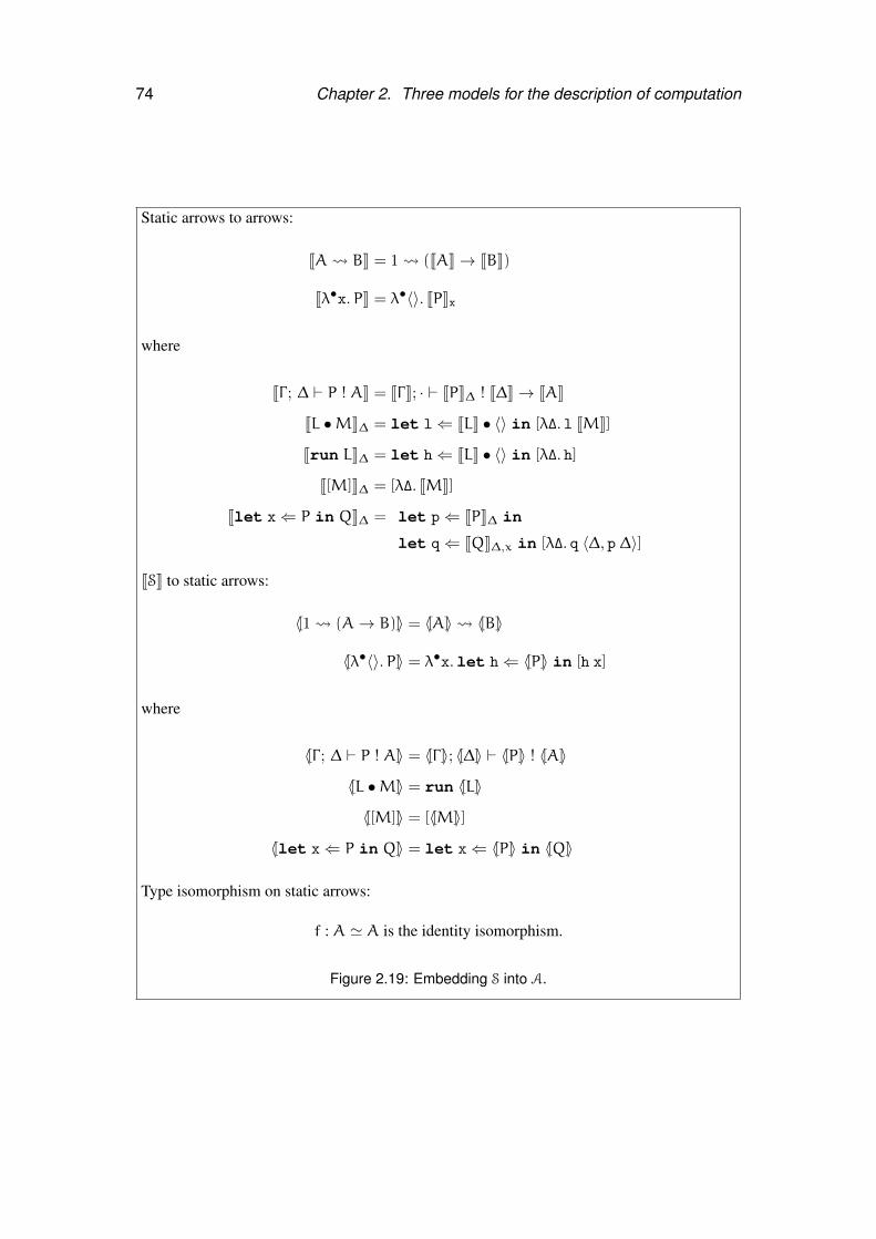
74 Chapter 2. Three models for the description of computation
Static arrows to arrows:
JA BK = 1 (JAK→ JBK)
Jλ•x.PK = λ•〈〉. JPKx
where
JΓ ; ∆ ` P ! AK = JΓK; · ` JPK∆ ! J∆K→ JAK
JL •MK∆ = let l⇐ JLK • 〈〉 in [λ∆. l JMK]
Jrun LK∆ = let h⇐ JLK • 〈〉 in [λ∆. h]
J[M]K∆ = [λ∆. JMK]
Jlet x⇐ P in QK∆ = let p⇐ JPK∆ in
let q⇐ JQK∆,x in [λ∆. q 〈∆, p ∆〉]
JSK to static arrows:
〈[1 (A→ B)]〉 = 〈[A]〉 〈[B]〉
〈[λ•〈〉.P]〉 = λ•x.let h⇐ 〈[P]〉 in [h x]
where
〈[Γ ; ∆ ` P ! A]〉 = 〈[Γ ]〉; 〈[∆]〉 ` 〈[P]〉 ! 〈[A]〉
〈[L •M]〉 = run 〈[L]〉
〈[[M]]〉 = [〈[M]〉]
〈[let x⇐ P in Q]〉 = let x⇐ 〈[P]〉 in 〈[Q]〉
Type isomorphism on static arrows:
f : A ' A is the identity isomorphism.
Figure 2.19: Embedding S into A.
2.4. Formal comparison of strength 75
Proof. By induction on the derivation of Q. There is one case for each command form. Ap-
pendix A.5.1 gives the proof in full.
Proposition 19. The translations J−K and 〈[−]〉 define an equational embedding of static arrows
into arrow calculus: S ↪→ A.
Proof. The equational embedding has three components:
• The eight laws of S follow from the five laws of A. The proof requires eight calculations,
one for each law of S. The cases for (β ) and (left) depend on Lemma 16, and the cases
for (assoc) and (run3) depend on Lemma 18.
• For terms in the image of the translation J−K, the five laws of A follow from the eight
laws of S. The proof requires five calculations, one for each law of A. The cases for
(β ) and (left) depend on Lemma 17
• Translating a termM from S into A and back is the identity:
〈[JMK]〉 =M
There is one case, for λ•x.Q. The proof involves showing a corresponding property for
commands. Translating a command P from S into A and back gives a term isomorphic
to λ•∆.P:
〈[JPK∆]〉 = run (λ•∆.P)
or, equivalently,
let d⇐ 〈[JPK∆]〉 in [d ∆] = P
There are four cases, one for each command form of S.
Appendix A.5 gives the proof in full.
In summary: idioms are equationally equivalent to static arrows, which embed into arrow
calculus (Figure 2.20).
2.4.2 Arrows and monads
Figure 2.21 defines the theory of monads, M, a straightforward recapitulation of the Haskell
interface presented in Section 2.2.1. Like I, M extends λ→×1 with a unary type constructor
M for computations of type MA which return a value of type A and two constants, return
and (>>=). There are three laws which, together with the laws of the lambda calculus, define
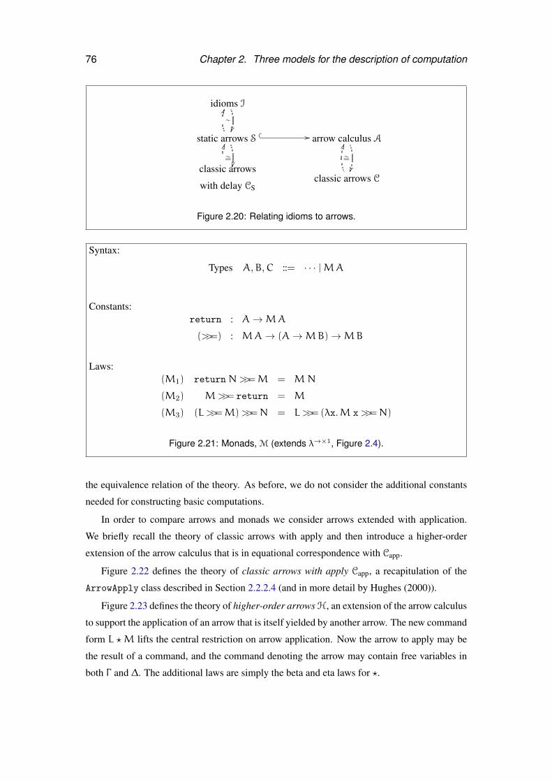
76 Chapter 2. Three models for the description of computation
idioms I
∼
static arrows S
HH
��
� � // arrow calculus A
∼=
classic arrows
with delay CS
∼=
II
classic arrows C
II
Figure 2.20: Relating idioms to arrows.
Syntax:
Types A,B,C ::= · · · |MA
Constants:return : A→MA
(>>=) : MA→ (A→MB)→MB
Laws:(M1) return N>>=M = MN
(M2) M>>= return = M
(M3) (L >>=M)>>=N = L >>= (λx.M x>>=N)
Figure 2.21: Monads, M (extends λ→×1, Figure 2.4).
the equivalence relation of the theory. As before, we do not consider the additional constants
needed for constructing basic computations.
In order to compare arrows and monads we consider arrows extended with application.
We briefly recall the theory of classic arrows with apply and then introduce a higher-order
extension of the arrow calculus that is in equational correspondence with Capp.
Figure 2.22 defines the theory of classic arrows with apply Capp, a recapitulation of the
ArrowApply class described in Section 2.2.2.4 (and in more detail by Hughes (2000)).
Figure 2.23 defines the theory of higher-order arrows H, an extension of the arrow calculus
to support the application of an arrow that is itself yielded by another arrow. The new command
form L ?M lifts the central restriction on arrow application. Now the arrow to apply may be
the result of a command, and the command denoting the arrow may contain free variables in
both Γ and ∆. The additional laws are simply the beta and eta laws for ?.
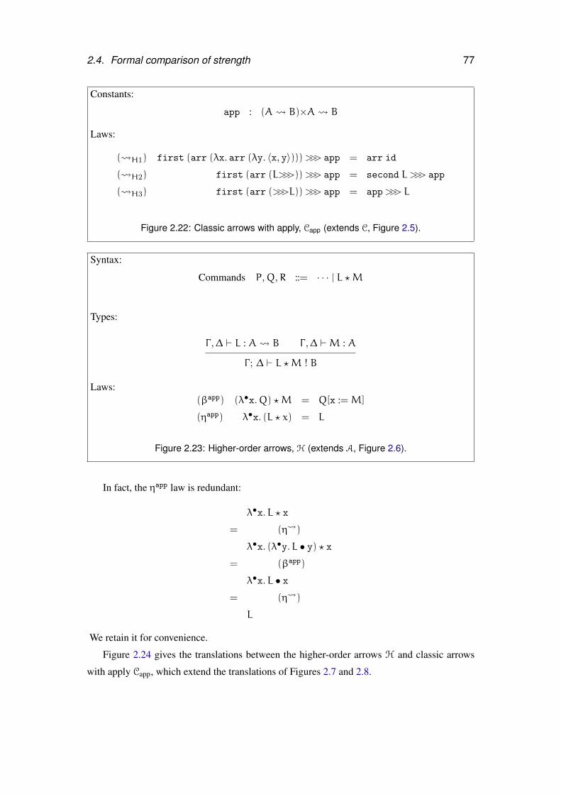
2.4. Formal comparison of strength 77
Constants:
app : (A B)×A B
Laws:
( H1) first (arr (λx. arr (λy. 〈x, y〉)))>>> app = arr id
( H2) first (arr (L>>>))>>> app = second L >>> app
( H3) first (arr (>>>L))>>> app = app>>> L
Figure 2.22: Classic arrows with apply, Capp (extends C, Figure 2.5).
Syntax:
Commands P,Q,R ::= · · · | L ?M
Types:
Γ ,∆ ` L : A B Γ ,∆ `M : A
Γ ; ∆ ` L ?M ! B
Laws:(βapp) (λ•x.Q) ?M = Q[x :=M]
(ηapp) λ•x. (L ? x) = L
Figure 2.23: Higher-order arrows, H (extends A, Figure 2.6).
In fact, the ηapp law is redundant:
λ•x.L ? x
= (η )
λ•x. (λ•y.L • y) ? x= (βapp)
λ•x.L • x= (η )
L
We retain it for convenience.
Figure 2.24 gives the translations between the higher-order arrows H and classic arrows
with apply Capp, which extend the translations of Figures 2.7 and 2.8.
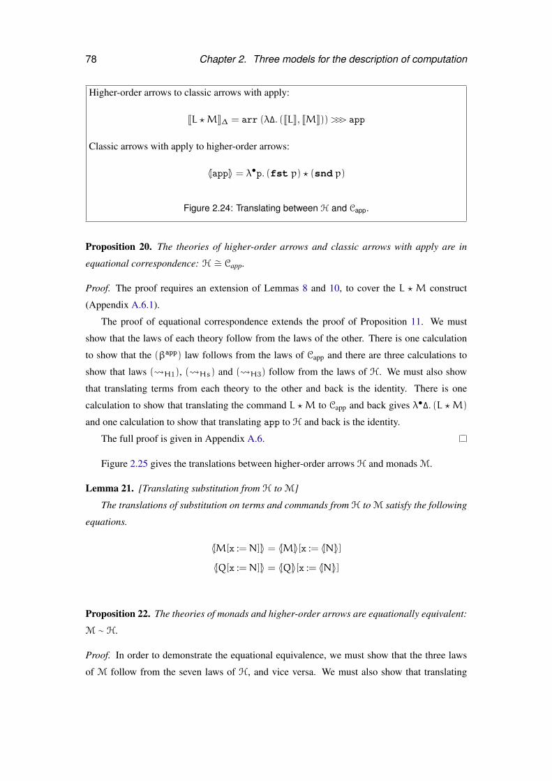
78 Chapter 2. Three models for the description of computation
Higher-order arrows to classic arrows with apply:
JL ?MK∆ = arr (λ∆. (JLK, JMK))>>> app
Classic arrows with apply to higher-order arrows:
〈[app]〉 = λ•p. (fst p) ? (snd p)
Figure 2.24: Translating between H and Capp.
Proposition 20. The theories of higher-order arrows and classic arrows with apply are in
equational correspondence: H ∼= Capp.
Proof. The proof requires an extension of Lemmas 8 and 10, to cover the L ?M construct
(Appendix A.6.1).
The proof of equational correspondence extends the proof of Proposition 11. We must
show that the laws of each theory follow from the laws of the other. There is one calculation
to show that the (βapp) law follows from the laws of Capp and there are three calculations to
show that laws ( H1), ( Hs) and ( H3) follow from the laws of H. We must also show
that translating terms from each theory to the other and back is the identity. There is one
calculation to show that translating the command L ?M to Capp and back gives λ•∆. (L ?M)
and one calculation to show that translating app to H and back is the identity.
The full proof is given in Appendix A.6.
Figure 2.25 gives the translations between higher-order arrows H and monads M.
Lemma 21. [Translating substitution from H to M]
The translations of substitution on terms and commands from H to M satisfy the following
equations.
〈[M[x :=N]]〉 = 〈[M]〉[x := 〈[N]〉]
〈[Q[x :=N]]〉 = 〈[Q]〉[x := 〈[N]〉]
Proposition 22. The theories of monads and higher-order arrows are equationally equivalent:
M ∼ H.
Proof. In order to demonstrate the equational equivalence, we must show that the three laws
of M follow from the seven laws of H, and vice versa. We must also show that translating
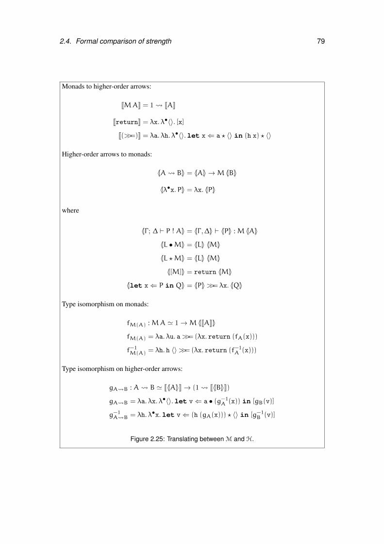
2.4. Formal comparison of strength 79
Monads to higher-order arrows:
JMAK = 1 JAK
JreturnK = λx. λ•〈〉. [x]
J(>>=)K = λa. λh. λ•〈〉.let x⇐ a ? 〈〉 in (h x) ? 〈〉
Higher-order arrows to monads:
〈[A B]〉 = 〈[A]〉 →M 〈[B]〉
〈[λ•x.P]〉 = λx. 〈[P]〉
where
〈[Γ ; ∆ ` P ! A]〉 = 〈[Γ ,∆]〉 ` 〈[P]〉 :M 〈[A]〉
〈[L •M]〉 = 〈[L]〉 〈[M]〉
〈[L ?M]〉 = 〈[L]〉 〈[M]〉
〈[[M]]〉 = return 〈[M]〉
〈[let x⇐ P in Q]〉 = 〈[P]〉>>= λx. 〈[Q]〉
Type isomorphism on monads:
fM(A) :MA ' 1→M 〈[JAK]〉
fM(A) = λa. λu. a>>= (λx. return (fA(x)))
f−1M(A) = λh. h 〈〉>>= (λx. return (f−1
A (x)))
Type isomorphism on higher-order arrows:
gA B : A B ' J〈[A]〉K→ (1 J〈[B]〉K)
gA B = λa. λx. λ•〈〉.let v⇐ a • (g−1A (x)) in [gB(v)]
g−1A B = λh. λ•x.let v⇐ (h (gA(x))) ? 〈〉 in [g−1
B (v)]
Figure 2.25: Translating between M and H.
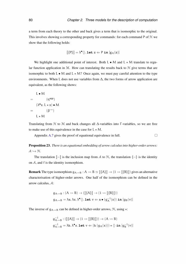
80 Chapter 2. Three models for the description of computation
a term from each theory to the other and back gives a term that is isomorphic to the original.
This involves showing a corresponding property for commands: for each command P of H we
show that the following holds:
J〈[P]〉K = λ•〈〉.let z⇐ P in [gA(z)]
We highlight one additional point of interest. Both L •M and L ?M translate to regu-
lar function application in M. How can translating the results back to H give terms that are
isomorphic to both L •M and L ?M? Once again, we must pay careful attention to the type
environments. When L does not use variables from ∆, the two forms of arrow application are
equivalent, as the following shows:
L •M= (ηapp)
(λ•x.L ? x) •M= (β )
L ?M
Translating from H to M and back changes all ∆-variables into Γ -variables, so we are free
to make use of this equivalence in the case for L ?M.
Appendix A.7 gives the proof of equational equivalence in full.
Proposition 23. There is an equational embedding of arrow calculus into higher-order arrows:
A ↪→ H.
The translation J−K is the inclusion map from A to H, the translation 〈[−]〉 is the identity
on A, and f is the identity isomorphism.
Remark The type isomorphism gA B : A B ' J〈[A]〉K→ (1 J〈[B]〉K) gives an alternative
characterisation of higher-order arrows. One half of the isomorphism can be defined in the
arrow calculus, A:
gA B : (A B)→ (J〈[A]〉K→ (1 J〈[B]〉K))
gA B = λa. λx. λ•〈〉.let v⇐ a • (g−1A (x)) in [gB(v)]
The inverse of gA B can be defined in higher-order arrows, H, using ?:
g−1A B : (J〈[A]〉K→ (1 J〈[B]〉K))→ (A B)
g−1A B = λh. λ•x.let v⇐ (h (gA(x))) ? 〈〉 in [g−1
B (v)]
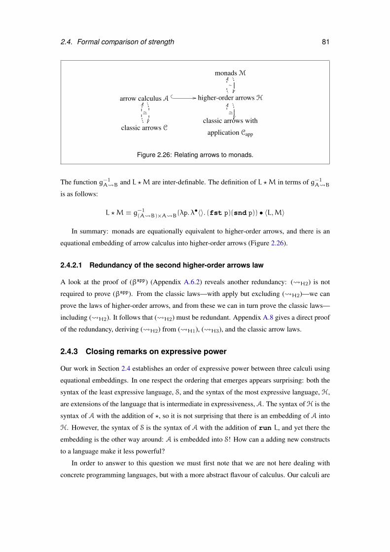
2.4. Formal comparison of strength 81
monads M
arrow calculus A
∼=
� � // higher-order arrows H
��
∼
II
classic arrows C
II
classic arrows with
application Capp
∼=
II
Figure 2.26: Relating arrows to monads.
The function g−1A B and L ?M are inter-definable. The definition of L ?M in terms of g−1
A B
is as follows:
L ?M ≡ g−1(A B)×A B(λp. λ•〈〉. (fst p)(snd p)) • 〈L,M〉
In summary: monads are equationally equivalent to higher-order arrows, and there is an
equational embedding of arrow calculus into higher-order arrows (Figure 2.26).
2.4.2.1 Redundancy of the second higher-order arrows law
A look at the proof of (βapp) (Appendix A.6.2) reveals another redundancy: ( H2) is not
required to prove (βapp). From the classic laws—with apply but excluding ( H2)—we can
prove the laws of higher-order arrows, and from these we can in turn prove the classic laws—
including ( H2). It follows that ( H2) must be redundant. Appendix A.8 gives a direct proof
of the redundancy, deriving ( H2) from ( H1), ( H3), and the classic arrow laws.
2.4.3 Closing remarks on expressive power
Our work in Section 2.4 establishes an order of expressive power between three calculi using
equational embeddings. In one respect the ordering that emerges appears surprising: both the
syntax of the least expressive language, S, and the syntax of the most expressive language, H,
are extensions of the language that is intermediate in expressiveness, A. The syntax of H is the
syntax of A with the addition of ?, so it is not surprising that there is an embedding of A into
H. However, the syntax of S is the syntax of A with the addition of run L, and yet there the
embedding is the other way around: A is embedded into S! How can a adding new constructs
to a language make it less powerful?
In order to answer to this question we must first note that we are not here dealing with
concrete programming languages, but with a more abstract flavour of calculus. Our calculi are
82 Chapter 2. Three models for the description of computation
not furnished with concrete value domains, or evaluation relations: each calculus admits many
possible interpretations, just as the various type classes in Section 2.2 have many instances.
Just as the laws associated with the type classes restrict the possible instances of the class,
so the equational theory of each calculus restricts which interpretations we can give to the
calculus. S extends not only the syntax, but also the equational theory of A, and it thereby
introduces further restrictions on the set of possible interpretations, so rendering the language
less powerful.
We can illustrate the principle using a more familiar calculus, and a rather extreme example.
In Figure 2.4 we gave the equational theory of a simply-typed lambda calculus λ→×1. Suppose
that we extend this calculus to obtain λ→×1⊥ , which has an additional constant ⊥A, and a law
(⊥) which equates every other term with this constant:
L,M,N ::= · · · | ⊥A
(⊥) ⊥A = L
Clearly only one-point value domains will be suitable for interpreting λ→×1⊥ : we have extended
the syntax of the language, but severely curtailed its expressive power.
Turning back to the relationship between arrow calculus, A, and static arrows, S, we can
show that there is no equational embedding corresponding to the syntax inclusion of A in S
by exhibiting terms that are equal in S but not in A, a circumstance which is forbidden by the
second criterion in our definition of equational embedding (Definition 7).
Lemma 24. Suppose b1 and b2 are distinct constants of base type B, and c is a constant of
type B 1. Let U and V be the following terms:
U = let x⇐ c • b1 in [〈〉]
V = let x⇐ c • b2 in [〈〉]
It can be shown that U = V in S.
Proof.
2.4. Formal comparison of strength 83
let x⇐ c • b1 in [〈〉]= (run1)
let x⇐ let f⇐ run c in [f b1] in [〈〉]= (assoc)
let f⇐ run c in let x⇐ [f b1] in [〈〉]= (left)
let f⇐ run c in [〈〉]= (left)
let f⇐ run c in let x⇐ [f b2] in [〈〉]= (assoc)
let x⇐ let f⇐ run c in [f b2] in [〈〉]= (run1)
let x⇐ c • b2 in [〈〉]
Lemma 25. Let U and V be defined as in Lemma 24. It cannot be shown that U = V in A.
Proof. We will show that U and V cannot be equated in A by interpreting A in the more
familiar setting of lambda calculus and showing that the interpretations of U and V are not
equal. Using the boolean state arrow to interpret , we set:
A B = Bool×A→ Bool× B
B = Bool
b1 = True
b2 = False
c3 = put (i.e. λp. 〈snd p, 〈〉〉)
and interpret the constructs of the arrow calculus using the translations of A into C (Figure 2.7)
and the standard definition of the state arrow (Section 2.2.2.2). Then U is interpreted as fol-
lows:
Jlet x⇐ put • True in [〈〉]K∆= (def J−K)
(arr id &&& (arr (λ∆. True)>>> put ))>>> arr (λ∆, x. 〈〉)= (def arr,>>>, &&&, etc.)
λ_. 〈True, 〈〉〉
and by an identical process V is interpreted as the term λ_. 〈False, 〈〉〉, which can evidently
not be equated with the interpretation of U.
84 Chapter 2. Three models for the description of computation
Proposition 26. The syntax inclusion of arrow calculus A into static arrows S does not form
an equational embedding.
Proof. If the syntax inclusion of A into S were an equational embedding then the equality
relations of A and S would coincide on terms that do not contain run L. However, Lemmas 24
and 25 show that the equality relation of S is strictly larger.
2.5 Future work
We have characterised idioms, monads and arrows as variations on a single calculus, establish-
ing the relative order of strength as idiom, arrow, monad in contrast to the putative order of
arrow, idiom, monad. The variations that bring the arrow calculus into correspondence with
idioms and with monads may be characterised either by type isomorphisms or by extensions to
the equational theory.
While the beta and eta laws of arrow calculus are more straightforward to work with than
the somewhat ad-hoc laws of classic arrows, relating the three interfaces by bringing each into
correspondence with a variant of arrow calculus is a somewhat circuitous route. It appears to
be possible to establish the relationships more directly, by presenting idioms and monads as
variants of classic arrows, in which the operators and laws of classic arrows are augmented
with the isomorphisms given above.
However, the arrow calculus has already proved useful independently of our investigations
here. Atkey (2008) draws inspiration from the arrow calculus to give a categorical semantics
for arrows; Vizzotto, Bois, and Sabry (2009) use the arrow calculus as the basis for a quantum
programming language.
Atkey has suggested an alternative formulation of static arrows in which the run construct
is replaced with a command-level lambda abstraction:
Γ ; ∆, x : A ` P ! B
Γ ; ∆ ` λ?x.P ! A→ B
together with beta and eta laws.
(βrun) let f⇐ λ?x.P in [fM] = P[x :=M]
(ηrun) λ?x.let f⇐ P in [f x] = P
This new form of abstraction and run are inter-definable.
λ?x.P = run (λ•x.P)
run L = λ?x.L • x
2.5. Future work 85
The duality of this approach is particularly appealing: static arrows add a new form of abstrac-
tion, while higher-order arrows add a new form of application. The laws of this new form of
abstraction also fit the standard pattern. However, there are apparent disadvantages to the pro-
posed laws: they appear less convenient to use, and it is not clear how to obtain rewrite rules
from them.
The arrow calculus is the analogue for arrows of Moggi’s computational metalanguage
(Moggi, 1991). A further direction for possible future investigation is an analogue for arrows
of Moggi’s (1989) computational lambda calculus.
Another unresolved question, raised in Section 2.2.3.2, is whether there are monads m
other than the environment monad for which α → m β ' m (α → β). For such instances
the idiom, arrow and monad interfaces are equivalently powerful (Proposition 15, Proposi-
tion 22).

Chapter 3
Abstracting controls 1
3.1 Introduction
Suppose we want to present users with an HTML form for entering a pair of dates (such as an
arrival and departure date for booking a hotel). In our initial design, we represent a date using
a single text field. Later, we choose to replace each date by a pair of pulldown menus, one to
select a month and one to select a day.
In typical web frameworks, such a change will require widespread modifications to the
code. Under the first design, the HTML form will contain two text fields, and the code that
handles the response will need to extract and parse the text entered in each field to yield a pair
of values of appropriate type, perhaps an abstract date type. Under the second design, however,
the HTML will contain four menus, and the code that handles the response will need to extract
the choices for each menu and combine them in pairs to yield each date.
How can we structure a program so that it is isolated from this choice? We want to capture
the notion of a part of a form, specifically a part for collecting values of a given type or purpose;
we call such an abstraction a formlet. The designer of the formlet should choose the HTML
presentation, and decide how to process the input into a date value. Clients of the formlet
should be insulated from the choice of HTML presentation, and also from the calculation that
yields the abstract value. And, of course, we should be able to compose formlets to build larger
formlets.
Once described, this sort of abstraction seems obvious and necessary. But remarkably
few web frameworks support it. Three existing web programming frameworks that do support
some degree of abstraction over form components are WASH (Thiemann, 2005), iData (Plas-
meijer and Achten, 2006) and WUI (Hanus, 2006, 2007), each having distinctive features and
1This chapter is a revision of Cooper et al. (2008a).
87
88 Chapter 3. Abstracting controls
limitations. (We discuss these further in Section 3.8.)
Our contribution is to reduce form abstraction to its essence. We show that a semantics
of formlets can be obtained by the composition of the three standard idioms that capture the
effects needed for form abstraction. We will further argue that while idioms are a good fit
for capturing form abstraction, monads and arrows are not. Furthermore, we illustrate how
the semantics can be extended to support additional features (such as checking form input for
validity), either by composing with additional standard idioms or by generalising to indexed
and parameterised idioms.
We will begin with an example, showing how formlets might appear to the programmer
(Section 3.2). Subsequent sections give a semantics in terms of idioms (Section 3.3), define
the syntactic sugar used throughout the chapter (Section 3.4), show how formlets fit into a web
programming environment (Section 3.5), and show how to extend the basic abstraction with
static XHTML validation and user-input validation (Section 3.6). We conclude by describing
a number of implementations of formlets in various languages (Section 3.7) and discussing
related work (Section 3.8).
Formlets can be implemented in any functional programming language; we present them
here in OCaml. OCaml is a particularly good fit for our exposition: we can give the semantics
in terms of idiom composition using functors and define the new syntactic forms using Camlp4,
the standard tool for extending OCaml syntax.
3.2 Formlets by example
Now we illustrate formlets, as they might appear to the programmer, with an example (Fig-
ure 3.1). We assume familiarity with HTML and OCaml. This section covers our OCaml
implementation, and so has features that may vary in another implementation of formlets. We
use a special syntax for programming with formlets, which is defined formally in Section 3.4;
this syntax is part of the implementation, and makes formlets easier to use, but is not an essen-
tial part of the abstraction.
The formlet date_formlet has two text input fields, labelled “Month” and “Day.” Upon
submission, this formlet will yield a date value representing the date entered. The user-defined
make_date function translates the day and month into a suitable representation.
A formlet expression consists of a body and a yields clause. The formlet expression
date_formlet has the body
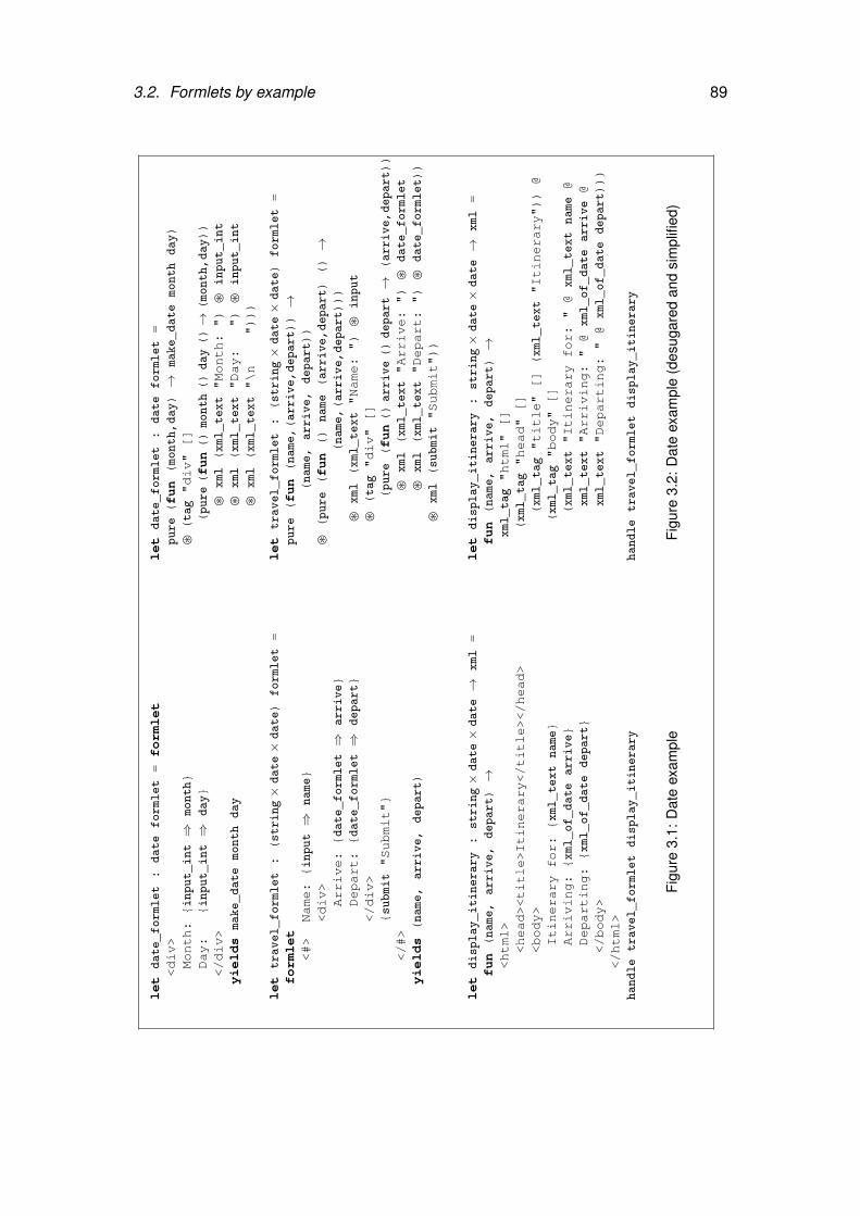
3.2. Formlets by example 89
let
date_formlet:
date
formlet=
formlet
<div>
Month:{input_int⇒
month}
Day:
{input_int⇒
day}
</div>
yields
make_date
month
day
let
travel_formlet:(string×
date×
date)
formlet=
formlet
<#>
Name:{input⇒
name}
<div>
Arrive:{date_formlet⇒
arrive}
Depart:{date_formlet⇒
depart}
</div>
{submit"Submit"}
</#>
yields(name,
arrive,
depart)
let
display_itinerary:
string×
date×
date→
xml=
fun(name,
arrive,
depart)→
<html>
<head><title>Itinerary</title></head>
<body>
Itineraryfor:{xml_text
name}
Arriving:{xml_of_date
arrive}
Departing:{xml_of_date
depart}
</body>
</html>
handle
travel_formlet
display_itinerary
Figu
re3.
1:D
ate
exam
ple
let
date_formlet:
date
formlet=
pure(fun(month,day)→
make_date
month
day)
�(tag"div"[]
(pure(fun()month()day()→
(month,day))
�xml(xml_text"Month:")
�input_int
�xml(xml_text"Day:
")
�input_int
�xml(xml_text"\n
")))
let
travel_formlet:(string×
date×
date)
formlet=
pure(fun(name,(arrive,depart))→
(name,
arrive,
depart))
�(pure(fun()
name(arrive,depart)()→
(name,(arrive,depart)))
�xml(xml_text"Name:")
�input
�(tag"div"[]
(pure(fun()arrive()depart→
(arrive,depart))
�xml(xml_text"Arrive:")
�date_formlet
�xml(xml_text"Depart:")
�date_formlet))
�xml(submit"Submit"))
let
display_itinerary:
string×
date×
date→
xml=
fun
(name,
arrive,
depart)→
xml_tag"html"[]
(xml_tag"head"[]
(xml_tag"title"[](xml_text"Itinerary"))@
(xml_tag"body"[]
(xml_text"Itineraryfor:"@
xml_text
name@
xml_text"Arriving:"@
xml_of_date
arrive@
xml_text"Departing:"@
xml_of_date
depart)))
handle
travel_formlet
display_itinerary
Figu
re3.
2:D
ate
exam
ple
(des
ugar
edan
dsi
mpl
ified
)
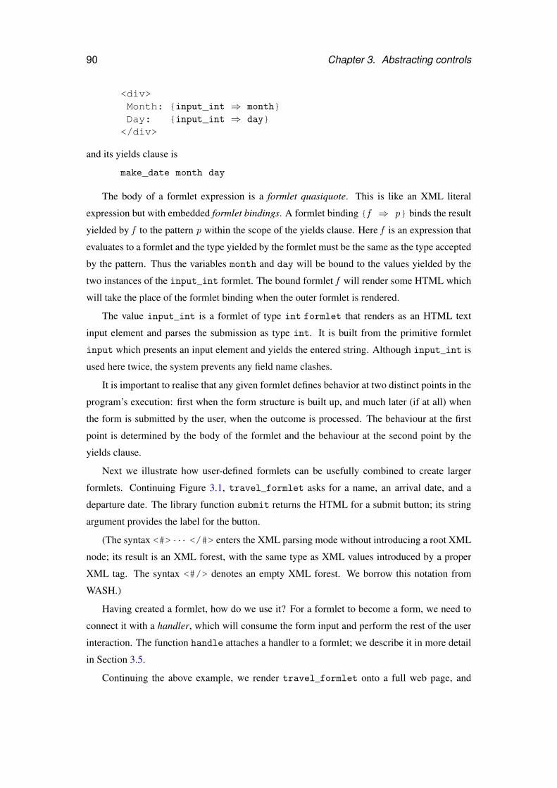
90 Chapter 3. Abstracting controls
<div>Month: {input_int ⇒ month}Day: {input_int ⇒ day}</div>
and its yields clause is
make_date month day
The body of a formlet expression is a formlet quasiquote. This is like an XML literal
expression but with embedded formlet bindings. A formlet binding {f ⇒ p} binds the result
yielded by f to the pattern p within the scope of the yields clause. Here f is an expression that
evaluates to a formlet and the type yielded by the formlet must be the same as the type accepted
by the pattern. Thus the variables month and day will be bound to the values yielded by the
two instances of the input_int formlet. The bound formlet f will render some HTML which
will take the place of the formlet binding when the outer formlet is rendered.
The value input_int is a formlet of type int formlet that renders as an HTML text
input element and parses the submission as type int. It is built from the primitive formlet
input which presents an input element and yields the entered string. Although input_int is
used here twice, the system prevents any field name clashes.
It is important to realise that any given formlet defines behavior at two distinct points in the
program’s execution: first when the form structure is built up, and much later (if at all) when
the form is submitted by the user, when the outcome is processed. The behaviour at the first
point is determined by the body of the formlet and the behaviour at the second point by the
yields clause.
Next we illustrate how user-defined formlets can be usefully combined to create larger
formlets. Continuing Figure 3.1, travel_formlet asks for a name, an arrival date, and a
departure date. The library function submit returns the HTML for a submit button; its string
argument provides the label for the button.
(The syntax <#> · · · </#> enters the XML parsing mode without introducing a root XML
node; its result is an XML forest, with the same type as XML values introduced by a proper
XML tag. The syntax <#/> denotes an empty XML forest. We borrow this notation from
WASH.)
Having created a formlet, how do we use it? For a formlet to become a form, we need to
connect it with a handler, which will consume the form input and perform the rest of the user
interaction. The function handle attaches a handler to a formlet; we describe it in more detail
in Section 3.5.
Continuing the above example, we render travel_formlet onto a full web page, and
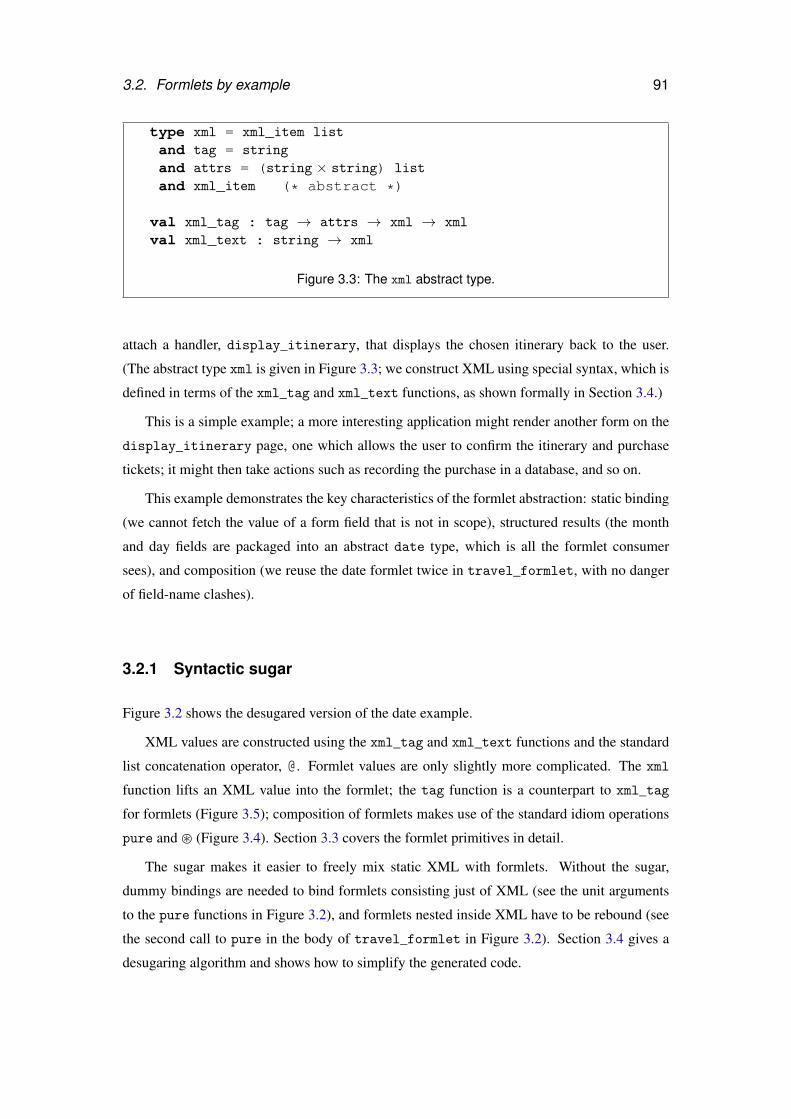
3.2. Formlets by example 91
type xml = xml_item list
and tag = string
and attrs = (string × string) list
and xml_item (* abstract *)
val xml_tag : tag → attrs → xml → xml
val xml_text : string → xml
Figure 3.3: The xml abstract type.
attach a handler, display_itinerary, that displays the chosen itinerary back to the user.
(The abstract type xml is given in Figure 3.3; we construct XML using special syntax, which is
defined in terms of the xml_tag and xml_text functions, as shown formally in Section 3.4.)
This is a simple example; a more interesting application might render another form on the
display_itinerary page, one which allows the user to confirm the itinerary and purchase
tickets; it might then take actions such as recording the purchase in a database, and so on.
This example demonstrates the key characteristics of the formlet abstraction: static binding
(we cannot fetch the value of a form field that is not in scope), structured results (the month
and day fields are packaged into an abstract date type, which is all the formlet consumer
sees), and composition (we reuse the date formlet twice in travel_formlet, with no danger
of field-name clashes).
3.2.1 Syntactic sugar
Figure 3.2 shows the desugared version of the date example.
XML values are constructed using the xml_tag and xml_text functions and the standard
list concatenation operator, @. Formlet values are only slightly more complicated. The xml
function lifts an XML value into the formlet; the tag function is a counterpart to xml_tag
for formlets (Figure 3.5); composition of formlets makes use of the standard idiom operations
pure and � (Figure 3.4). Section 3.3 covers the formlet primitives in detail.
The sugar makes it easier to freely mix static XML with formlets. Without the sugar,
dummy bindings are needed to bind formlets consisting just of XML (see the unit arguments
to the pure functions in Figure 3.2), and formlets nested inside XML have to be rebound (see
the second call to pure in the body of travel_formlet in Figure 3.2). Section 3.4 gives a
desugaring algorithm and shows how to simplify the generated code.
92 Chapter 3. Abstracting controls
3.2.2 Life without formlets
Now consider implementing the above example using the standard HTML/CGI interface. We
would face the following difficulties with the standard interface:
• There is no static association between a form definition and the code that handles it,
so the interface is fragile. This means the form and the handling code need to be kept
manually in sync.
• Field values are always received individually and always as strings: the interface pro-
vides no facility for processing data or giving it structure.
• Given two forms, there is generally no easy way to combine them into a new form with-
out danger of name clashes amongst the fields—thus it is not easy to write a form that
abstractly uses subcomponents. In particular, using a form twice within a larger form is
difficult.
Conventional web programming frameworks such as PHP (PHP) and Ruby on Rails (Hans-
son, 2008) enable abstraction only through templating or textual substitution, hence there is
no automatic way to generate fresh field names, and any form “abstraction” (such as a tem-
plate) still exposes the programmer to the concrete field names used in the form. Even ad-
vanced systems such as PLT Scheme (Graunke et al., 2001b), JWIG (Christensen et al., 2003),
scriptlets (Elsman and Larsen, 2004), Ocsigen (Balat, 2006), Lift (lif, 2008) and the original
design for Links (Cooper et al., 2006) all fall short in the same way.
Formlets address all of the above problems: they provide a static association between a
form and its handler (ensuring that fields referenced actually exist and are of the right type),
they allow processing raw form data into structured values, and they allow composition, in part
by generating fresh field names at runtime.
3.3 Semantics
We wish to give a semantics of formlets using a well-understood formalism. We shall show
that formlets conform to the idiom interface described in Section 2.2.3. We begin with a con-
crete implementation in OCaml, which we then factor using standard idioms to give a formal
semantics.
Figure 3.4 gives the idiom interface in OCaml.
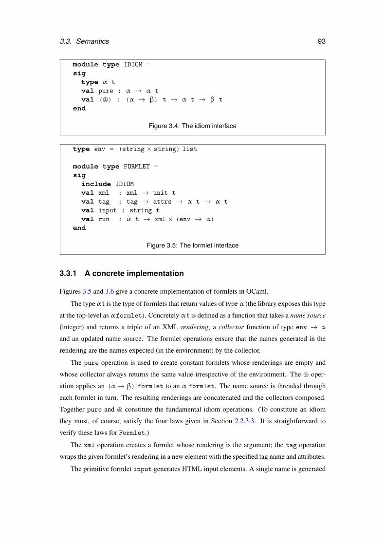
3.3. Semantics 93
module type IDIOM =sigtype α t
val pure : α → α t
val (�) : (α → β) t → α t → β t
end
Figure 3.4: The idiom interface
type env = (string × string) list
module type FORMLET =sig
include IDIOM
val xml : xml → unit t
val tag : tag → attrs → α t → α t
val input : string t
val run : α t → xml × (env → α)end
Figure 3.5: The formlet interface
3.3.1 A concrete implementation
Figures 3.5 and 3.6 give a concrete implementation of formlets in OCaml.
The type αt is the type of formlets that return values of type α (the library exposes this type
at the top-level as αformlet). Concretely αt is defined as a function that takes a name source
(integer) and returns a triple of an XML rendering, a collector function of type env → α
and an updated name source. The formlet operations ensure that the names generated in the
rendering are the names expected (in the environment) by the collector.
The pure operation is used to create constant formlets whose renderings are empty and
whose collector always returns the same value irrespective of the environment. The � oper-
ation applies an (α→ β) formlet to an α formlet. The name source is threaded through
each formlet in turn. The resulting renderings are concatenated and the collectors composed.
Together pure and � constitute the fundamental idiom operations. (To constitute an idiom
they must, of course, satisfy the four laws given in Section 2.2.3.3. It is straightforward to
verify these laws for Formlet.)
The xml operation creates a formlet whose rendering is the argument; the tag operation
wraps the given formlet’s rendering in a new element with the specified tag name and attributes.
The primitive formlet input generates HTML input elements. A single name is generated
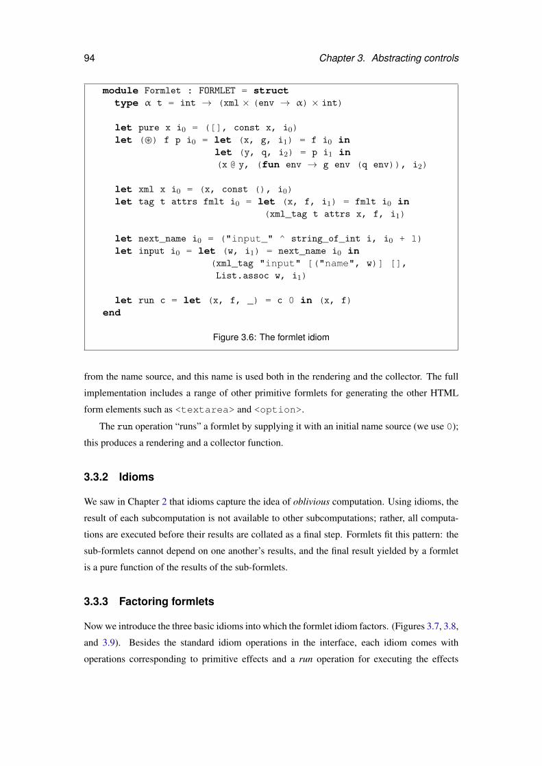
94 Chapter 3. Abstracting controls
module Formlet : FORMLET = structtype α t = int → (xml × (env → α) × int)
let pure x i0 = ([], const x, i0)let (�) f p i0 = let (x, g, i1) = f i0 in
let (y, q, i2) = p i1 in(x @ y, (fun env → g env (q env)), i2)
let xml x i0 = (x, const (), i0)let tag t attrs fmlt i0 = let (x, f, i1) = fmlt i0 in
(xml_tag t attrs x, f, i1)
let next_name i0 = ("input_" ^ string_of_int i, i0 + 1)let input i0 = let (w, i1) = next_name i0 in
(xml_tag "input" [("name", w)] [],List.assoc w, i1)
let run c = let (x, f, _) = c 0 in (x, f)end
Figure 3.6: The formlet idiom
from the name source, and this name is used both in the rendering and the collector. The full
implementation includes a range of other primitive formlets for generating the other HTML
form elements such as <textarea> and <option>.
The run operation “runs” a formlet by supplying it with an initial name source (we use 0);
this produces a rendering and a collector function.
3.3.2 Idioms
We saw in Chapter 2 that idioms capture the idea of oblivious computation. Using idioms, the
result of each subcomputation is not available to other subcomputations; rather, all computa-
tions are executed before their results are collated as a final step. Formlets fit this pattern: the
sub-formlets cannot depend on one another’s results, and the final result yielded by a formlet
is a pure function of the results of the sub-formlets.
3.3.3 Factoring formlets
Now we introduce the three basic idioms into which the formlet idiom factors. (Figures 3.7, 3.8,
and 3.9). Besides the standard idiom operations in the interface, each idiom comes with
operations corresponding to primitive effects and a run operation for executing the effects
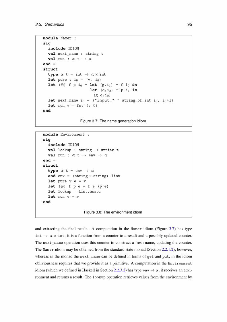
3.3. Semantics 95
module Namer :siginclude IDIOM
val next_name : string t
val run : α t → α
end =struct
type α t = int → α × int
let pure v i0 = (v, i0)let (�) f p i0 = let (g,i1) = f i0 in
let (q,i2) = p i1 in(g q,i2)
let next_name i0 = ("input_" ^ string_of_int i0, i0+1)let run v = fst (v 0)
end
Figure 3.7: The name generation idiom
module Environment :siginclude IDIOM
val lookup : string → string t
val run : α t → env → α
end =structtype α t = env → α
and env = (string × string) list
let pure v e = v
let (�) f p e = f e (p e)let lookup = List.assoclet run v = v
end
Figure 3.8: The environment idiom
and extracting the final result. A computation in the Namer idiom (Figure 3.7) has type
int → α × int; it is a function from a counter to a result and a possibly-updated counter.
The next_name operation uses this counter to construct a fresh name, updating the counter.
The Namer idiom may be obtained from the standard state monad (Section 2.2.1.2); however,
whereas in the monad the next_name can be defined in terms of get and put, in the idiom
obliviousness requires that we provide it as a primitive. A computation in the Environment
idiom (which we defined in Haskell in Section 2.2.3.2) has type env→ α; it receives an envi-
ronment and returns a result. The lookup operation retrieves values from the environment by
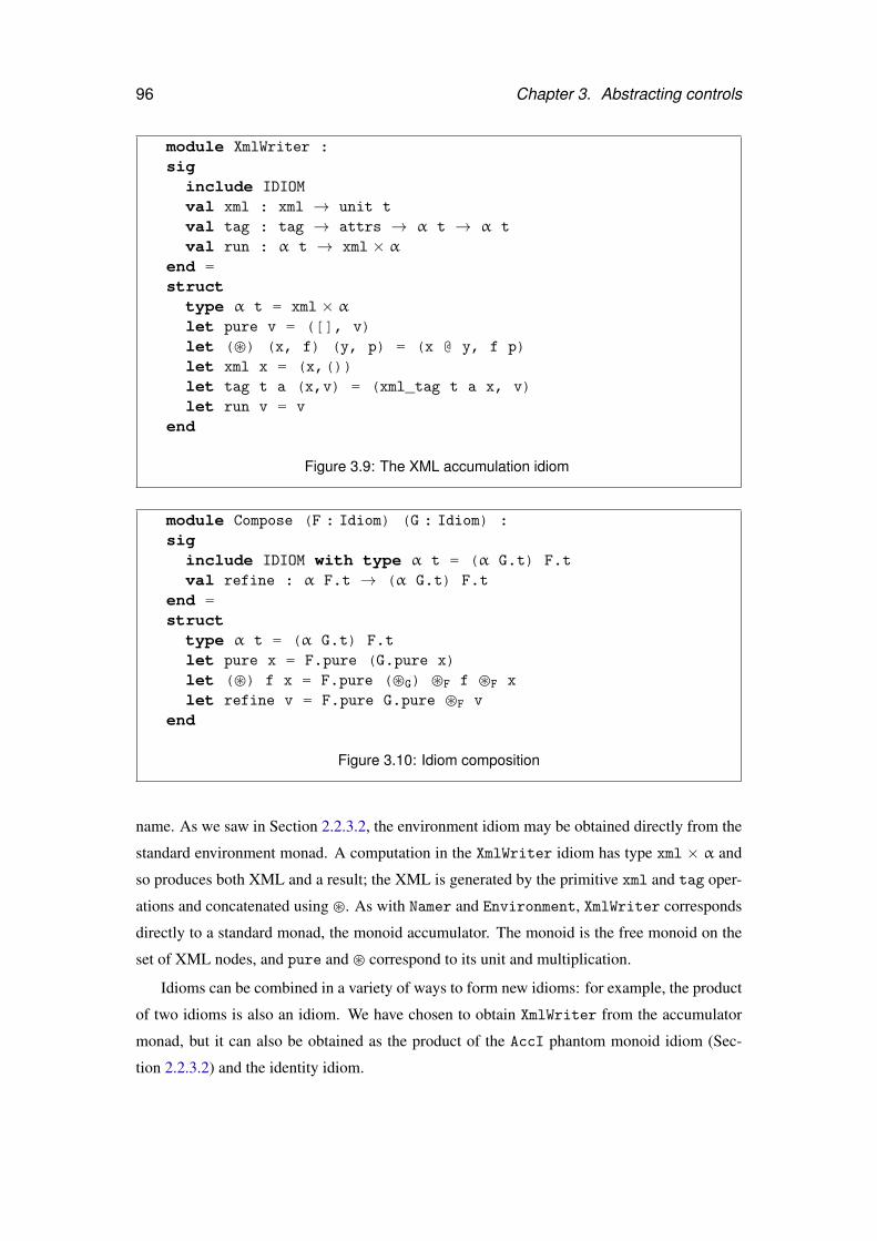
96 Chapter 3. Abstracting controls
module XmlWriter :siginclude IDIOM
val xml : xml → unit t
val tag : tag → attrs → α t → α t
val run : α t → xml × αend =struct
type α t = xml × αlet pure v = ([], v)let (�) (x, f) (y, p) = (x @ y, f p)let xml x = (x,())let tag t a (x,v) = (xml_tag t a x, v)let run v = v
end
Figure 3.9: The XML accumulation idiom
module Compose (F : Idiom) (G : Idiom) :sig
include IDIOM with type α t = (α G.t) F.tval refine : α F.t → (α G.t) F.t
end =struct
type α t = (α G.t) F.tlet pure x = F.pure (G.pure x)let (�) f x = F.pure (�G) �F f �F x
let refine v = F.pure G.pure �F v
end
Figure 3.10: Idiom composition
name. As we saw in Section 2.2.3.2, the environment idiom may be obtained directly from the
standard environment monad. A computation in the XmlWriter idiom has type xml × α and
so produces both XML and a result; the XML is generated by the primitive xml and tag oper-
ations and concatenated using �. As with Namer and Environment, XmlWriter corresponds
directly to a standard monad, the monoid accumulator. The monoid is the free monoid on the
set of XML nodes, and pure and � correspond to its unit and multiplication.
Idioms can be combined in a variety of ways to form new idioms: for example, the product
of two idioms is also an idiom. We have chosen to obtain XmlWriter from the accumulator
monad, but it can also be obtained as the product of the AccI phantom monoid idiom (Sec-
tion 2.2.3.2) and the identity idiom.
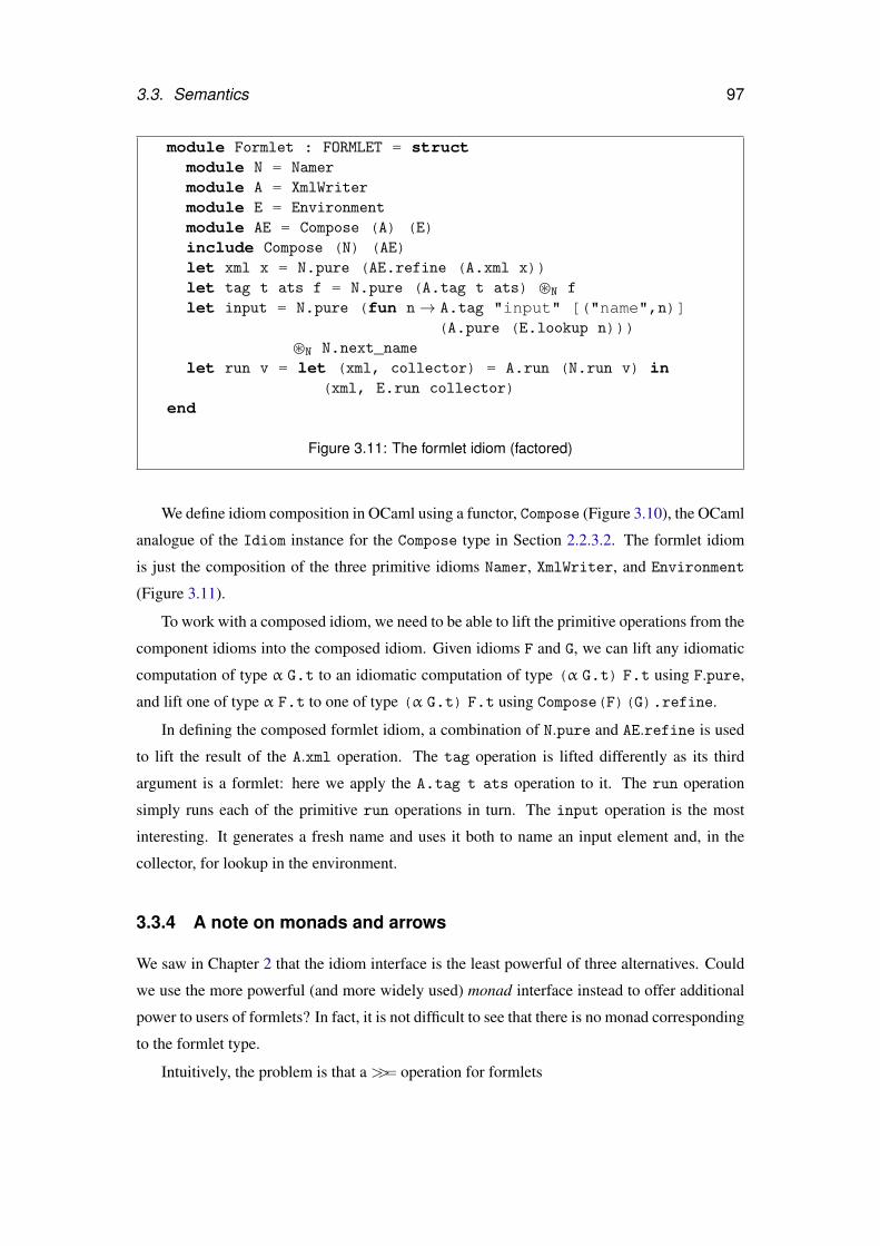
3.3. Semantics 97
module Formlet : FORMLET = structmodule N = Namer
module A = XmlWriter
module E = Environment
module AE = Compose (A) (E)include Compose (N) (AE)let xml x = N.pure (AE.refine (A.xml x))let tag t ats f = N.pure (A.tag t ats) �N f
let input = N.pure (fun n→ A.tag "input" [("name",n)](A.pure (E.lookup n)))
�N N.next_namelet run v = let (xml, collector) = A.run (N.run v) in
(xml, E.run collector)end
Figure 3.11: The formlet idiom (factored)
We define idiom composition in OCaml using a functor, Compose (Figure 3.10), the OCaml
analogue of the Idiom instance for the Compose type in Section 2.2.3.2. The formlet idiom
is just the composition of the three primitive idioms Namer, XmlWriter, and Environment
(Figure 3.11).
To work with a composed idiom, we need to be able to lift the primitive operations from the
component idioms into the composed idiom. Given idioms F and G, we can lift any idiomatic
computation of type α G.t to an idiomatic computation of type (α G.t) F.t using F.pure,
and lift one of type α F.t to one of type (α G.t) F.t using Compose(F)(G).refine.
In defining the composed formlet idiom, a combination of N.pure and AE.refine is used
to lift the result of the A.xml operation. The tag operation is lifted differently as its third
argument is a formlet: here we apply the A.tag t ats operation to it. The run operation
simply runs each of the primitive run operations in turn. The input operation is the most
interesting. It generates a fresh name and uses it both to name an input element and, in the
collector, for lookup in the environment.
3.3.4 A note on monads and arrows
We saw in Chapter 2 that the idiom interface is the least powerful of three alternatives. Could
we use the more powerful (and more widely used) monad interface instead to offer additional
power to users of formlets? In fact, it is not difficult to see that there is no monad corresponding
to the formlet type.
Intuitively, the problem is that a >>= operation for formlets
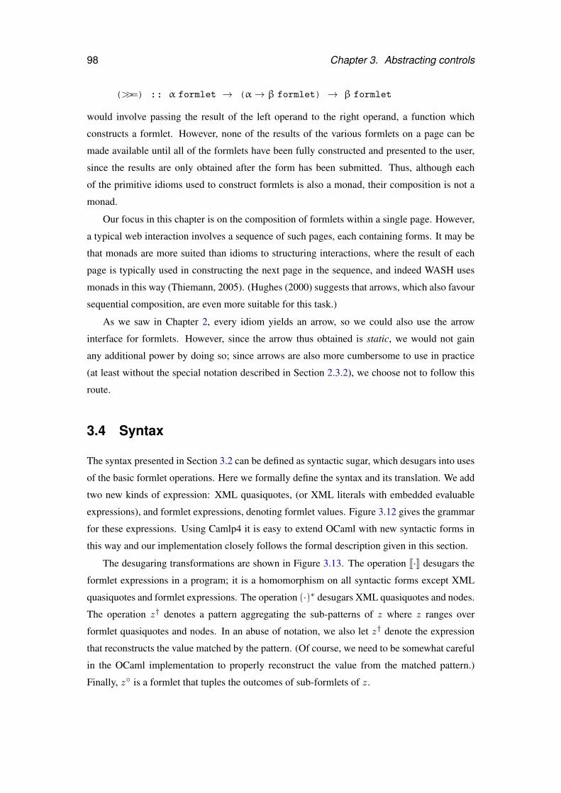
98 Chapter 3. Abstracting controls
(>>=) :: α formlet → (α→ β formlet) → β formlet
would involve passing the result of the left operand to the right operand, a function which
constructs a formlet. However, none of the results of the various formlets on a page can be
made available until all of the formlets have been fully constructed and presented to the user,
since the results are only obtained after the form has been submitted. Thus, although each
of the primitive idioms used to construct formlets is also a monad, their composition is not a
monad.
Our focus in this chapter is on the composition of formlets within a single page. However,
a typical web interaction involves a sequence of such pages, each containing forms. It may be
that monads are more suited than idioms to structuring interactions, where the result of each
page is typically used in constructing the next page in the sequence, and indeed WASH uses
monads in this way (Thiemann, 2005). (Hughes (2000) suggests that arrows, which also favour
sequential composition, are even more suitable for this task.)
As we saw in Chapter 2, every idiom yields an arrow, so we could also use the arrow
interface for formlets. However, since the arrow thus obtained is static, we would not gain
any additional power by doing so; since arrows are also more cumbersome to use in practice
(at least without the special notation described in Section 2.3.2), we choose not to follow this
route.
3.4 Syntax
The syntax presented in Section 3.2 can be defined as syntactic sugar, which desugars into uses
of the basic formlet operations. Here we formally define the syntax and its translation. We add
two new kinds of expression: XML quasiquotes, (or XML literals with embedded evaluable
expressions), and formlet expressions, denoting formlet values. Figure 3.12 gives the grammar
for these expressions. Using Camlp4 it is easy to extend OCaml with new syntactic forms in
this way and our implementation closely follows the formal description given in this section.
The desugaring transformations are shown in Figure 3.13. The operation J·K desugars the
formlet expressions in a program; it is a homomorphism on all syntactic forms except XML
quasiquotes and formlet expressions. The operation (·)∗ desugars XML quasiquotes and nodes.
The operation z † denotes a pattern aggregating the sub-patterns of z where z ranges over
formlet quasiquotes and nodes. In an abuse of notation, we also let z † denote the expression
that reconstructs the value matched by the pattern. (Of course, we need to be somewhat careful
in the OCaml implementation to properly reconstruct the value from the matched pattern.)
Finally, z◦ is a formlet that tuples the outcomes of sub-formlets of z .
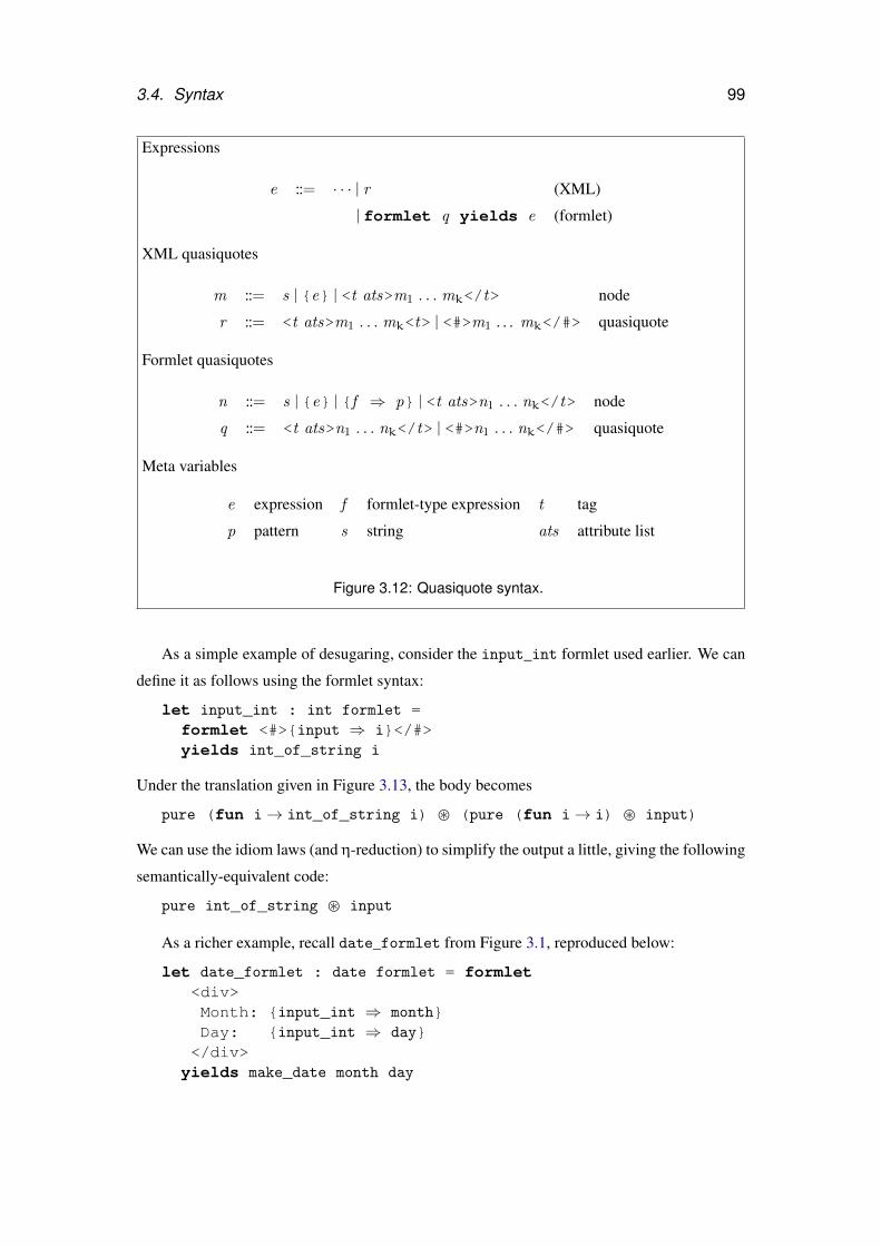
3.4. Syntax 99
Expressions
e ::= · · · | r (XML)
| formlet q yields e (formlet)
XML quasiquotes
m ::= s | {e} | <t ats>m1 . . . mk</t> node
r ::= <t ats>m1 . . . mk<t> | <#>m1 . . . mk</#> quasiquote
Formlet quasiquotes
n ::= s | {e} | {f ⇒ p} | <t ats>n1 . . . nk</t> node
q ::= <t ats>n1 . . . nk</t> | <#>n1 . . . nk</#> quasiquote
Meta variables
e expression f formlet-type expression t tag
p pattern s string ats attribute list
Figure 3.12: Quasiquote syntax.
As a simple example of desugaring, consider the input_int formlet used earlier. We can
define it as follows using the formlet syntax:
let input_int : int formlet =formlet <#>{input ⇒ i}</#>yields int_of_string i
Under the translation given in Figure 3.13, the body becomes
pure (fun i→ int_of_string i) � (pure (fun i→ i) � input)
We can use the idiom laws (and η-reduction) to simplify the output a little, giving the following
semantically-equivalent code:
pure int_of_string � input
As a richer example, recall date_formlet from Figure 3.1, reproduced below:
let date_formlet : date formlet = formlet<div>Month: {input_int ⇒ month}Day: {input_int ⇒ day}</div>
yields make_date month day
100 Chapter 3. Abstracting controls
JrK = r∗
Jformlet q yields eK = pure (fun q† → JeK) � q◦
s∗ = xml_text s
{e}∗ = JeK
(<t ats>m1 . . . mk</t>)∗ = xml_tag t ats (<#>m1 . . . mk</#>)∗
(<#>m1 . . . mk</#>)∗ = m∗1 @ · · · @ m∗k
s◦ = xml (xml_text s)
{e}◦ = xml JeK
{f ⇒ p}◦ = Jf K
(<t ats>n1 . . . nk</t>)◦ = tag t ats (<#>n1 . . . nk</#>)◦
(<#>n1 . . . nk</#>)◦ = pure (fun n†1 . . . n†k → (n†1, . . . ,n†k))
�n◦1 . . . � n◦k
s† = ()
{e}† = ()
{f ⇒ p}† = p
(<t ats>n1 . . . nk</t>)† = (n†1 , . . . , n†k)
(<#>n1 . . . nk</#>)† = (n†1 , . . . , n†k)
Figure 3.13: Desugaring XML and formlets.
In this case the desugaring algorithm produces the following output:
let date_formlet : date formlet =pure (fun ((),month,(),day,()) → make_date month day)� (tag "div" []
(pure (fun () month () day ()→ ((),month,(),day,()))� xml (xml_text "Month: ") � input_int� xml (xml_text "Day: ") � input_int� xml (xml_text "\n ")))
It is easy to optimise this code by removing the extra units from the body of the inner pure and
from the arguments to the function in the outer pure, and we have applied this minor optimi-
sation in the simplified version given in Figure 3.2. However, the code is still rather inefficient:
in particular, the variables month and day are rebound in each pure function. Similarly, in
the travel_formlet of Figure 3.2 the variables arrive and depart are bound three times.
3.5. Pragmatics 101
Section 3.6.3 outlines an alternate desugaring that obviates this rebinding.
3.4.1 Completeness
The formlet syntax is complete: everything expressible with the formlet operations can be
expressed directly in the syntax. For example, the � operator of the formlet idiom may be
written as a function ap using syntactic sugar:
let ap : (α → β) formlet → α formlet → β formlet =fun f p → formlet <#>{f ⇒ g}{p ⇒ q}</#> yields g q
Under the desugaring transformation, the body becomes
(pure (fun (g,q)→ g q)) � (pure (fun g q→ (g,q)) � f � p)
which, under the idiom laws, is equivalent to f � p. And pure, too, can be defined in the
sugar:
let pure : α → α formlet =fun x→ formlet <#/> yields x
In this case desugaring produces the following code for the body:
pure (fun ()→ x) � pure ()
which is equal to pure x under the homomorphism law for idioms.
3.5 Pragmatics
We now consider the practicalities of using formlets in a typical web programming environ-
ment. We assume that the runtime system provides the following functions:
val pickle_cont : (α → β) → string
val unpickle_cont : string → (α → β)val cgi_args : unit → env
val send_document : xml → unit
The first two, pickle_cont, and unpickle_cont, convert a function to and from a tex-
tual representation. We leave the details of the operation of these functions unspecified: for
example, pickle_cont might serialise the code underlying the function to a string, or store
the function in a table and return a string that acts as a key into the table. (We describe the
approach taken in Links in the next chapter.) We will use pickle_cont and unpickle_cont
to persist continuation functions for formlets across requests. The types are inherently unsafe:
there is nothing in the types of the functions to prevent the caller from pickling a function at
one type and unpickling it at another.
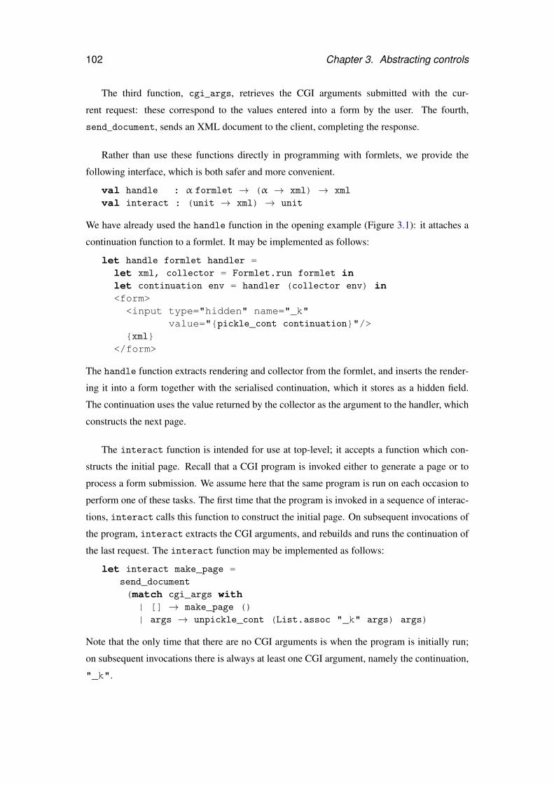
102 Chapter 3. Abstracting controls
The third function, cgi_args, retrieves the CGI arguments submitted with the cur-
rent request: these correspond to the values entered into a form by the user. The fourth,
send_document, sends an XML document to the client, completing the response.
Rather than use these functions directly in programming with formlets, we provide the
following interface, which is both safer and more convenient.
val handle : α formlet → (α → xml) → xml
val interact : (unit → xml) → unit
We have already used the handle function in the opening example (Figure 3.1): it attaches a
continuation function to a formlet. It may be implemented as follows:
let handle formlet handler =let xml, collector = Formlet.run formlet inlet continuation env = handler (collector env) in<form>
<input type="hidden" name="_k"value="{pickle_cont continuation}"/>
{xml}</form>
The handle function extracts rendering and collector from the formlet, and inserts the render-
ing it into a form together with the serialised continuation, which it stores as a hidden field.
The continuation uses the value returned by the collector as the argument to the handler, which
constructs the next page.
The interact function is intended for use at top-level; it accepts a function which con-
structs the initial page. Recall that a CGI program is invoked either to generate a page or to
process a form submission. We assume here that the same program is run on each occasion to
perform one of these tasks. The first time that the program is invoked in a sequence of interac-
tions, interact calls this function to construct the initial page. On subsequent invocations of
the program, interact extracts the CGI arguments, and rebuilds and runs the continuation of
the last request. The interact function may be implemented as follows:
let interact make_page =send_document(match cgi_args with
| [] → make_page ()| args → unpickle_cont (List.assoc "_k" args) args)
Note that the only time that there are no CGI arguments is when the program is initially run;
on subsequent invocations there is always at least one CGI argument, namely the continuation,
"_k".
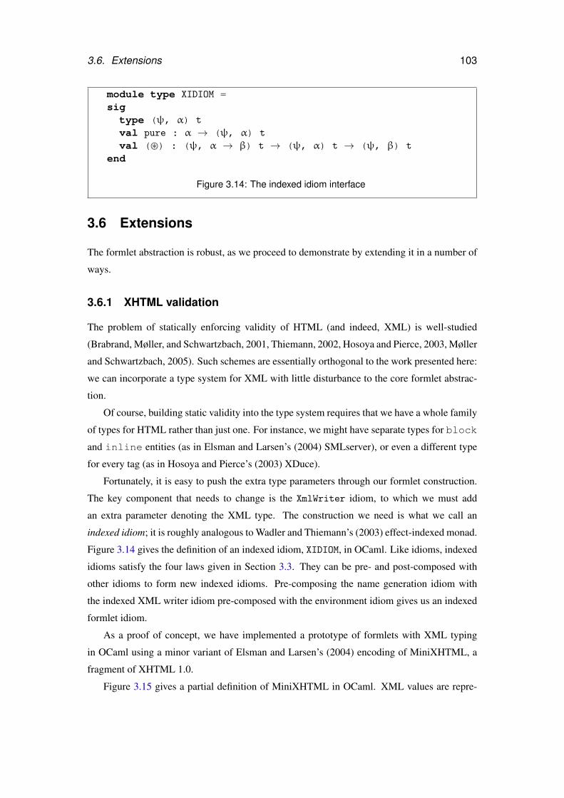
3.6. Extensions 103
module type XIDIOM =sigtype (ψ, α) t
val pure : α → (ψ, α) t
val (�) : (ψ, α → β) t → (ψ, α) t → (ψ, β) t
end
Figure 3.14: The indexed idiom interface
3.6 Extensions
The formlet abstraction is robust, as we proceed to demonstrate by extending it in a number of
ways.
3.6.1 XHTML validation
The problem of statically enforcing validity of HTML (and indeed, XML) is well-studied
(Brabrand, Møller, and Schwartzbach, 2001, Thiemann, 2002, Hosoya and Pierce, 2003, Møller
and Schwartzbach, 2005). Such schemes are essentially orthogonal to the work presented here:
we can incorporate a type system for XML with little disturbance to the core formlet abstrac-
tion.
Of course, building static validity into the type system requires that we have a whole family
of types for HTML rather than just one. For instance, we might have separate types for block
and inline entities (as in Elsman and Larsen’s (2004) SMLserver), or even a different type
for every tag (as in Hosoya and Pierce’s (2003) XDuce).
Fortunately, it is easy to push the extra type parameters through our formlet construction.
The key component that needs to change is the XmlWriter idiom, to which we must add
an extra parameter denoting the XML type. The construction we need is what we call an
indexed idiom; it is roughly analogous to Wadler and Thiemann’s (2003) effect-indexed monad.
Figure 3.14 gives the definition of an indexed idiom, XIDIOM, in OCaml. Like idioms, indexed
idioms satisfy the four laws given in Section 3.3. They can be pre- and post-composed with
other idioms to form new indexed idioms. Pre-composing the name generation idiom with
the indexed XML writer idiom pre-composed with the environment idiom gives us an indexed
formlet idiom.
As a proof of concept, we have implemented a prototype of formlets with XML typing
in OCaml using a minor variant of Elsman and Larsen’s (2004) encoding of MiniXHTML, a
fragment of XHTML 1.0.
Figure 3.15 gives a partial definition of MiniXHTML in OCaml. XML values are repre-
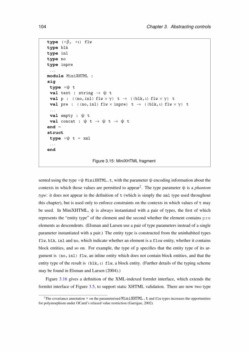
104 Chapter 3. Abstracting controls
type (+β, +ι) flw
type blk
type inl
type no
type inpre
. . .module MiniXHTML :sigtype +ψ t
val text : string → ψ t
val p : ((no,inl) flw × γ) t → ((blk,ι) flw × γ) t
val pre : ((no,inl) flw × inpre) t → ((blk,ι) flw × γ) t
. . .val empty : ψ t
val concat : ψ t → ψ t → ψ t
end =structtype +ψ t = xml
. . .end
Figure 3.15: MiniXHTML fragment
sented using the type +ψ MiniXHTML.t, with the parameterψ encoding information about the
contexts in which those values are permitted to appear2. The type parameter ψ is a phantom
type: it does not appear in the definition of t (which is simply the xml type used throughout
this chapter), but is used only to enforce constraints on the contexts in which values of t may
be used. In MiniXHTML, ψ is always instantiated with a pair of types, the first of which
represents the “entity type” of the element and the second whether the element contains pre
elements as descendents. (Elsman and Larsen use a pair of type parameters instead of a single
parameter instantiated with a pair.) The entity type is constructed from the uninhabited types
flw, blk, inl and no, which indicate whether an element is a flow entity, whether it contains
block entities, and so on. For example, the type of p specifies that the entity type of its ar-
gument is (no,inl) flw, an inline entity which does not contain block entities, and that the
entity type of the result is (blk,ι) flw, a block entity. (Further details of the typing scheme
may be found in Elsman and Larsen (2004).)
Figure 3.16 gives a definition of the XML-indexed formlet interface, which extends the
formlet interface of Figure 3.5, to support static XHTML validation. There are now two type
2The covariance annotation + on the parameterised MiniXHTML.t and flw types increases the opportunitiesfor polymorphism under OCaml’s relaxed value restriction (Garrigue, 2002).
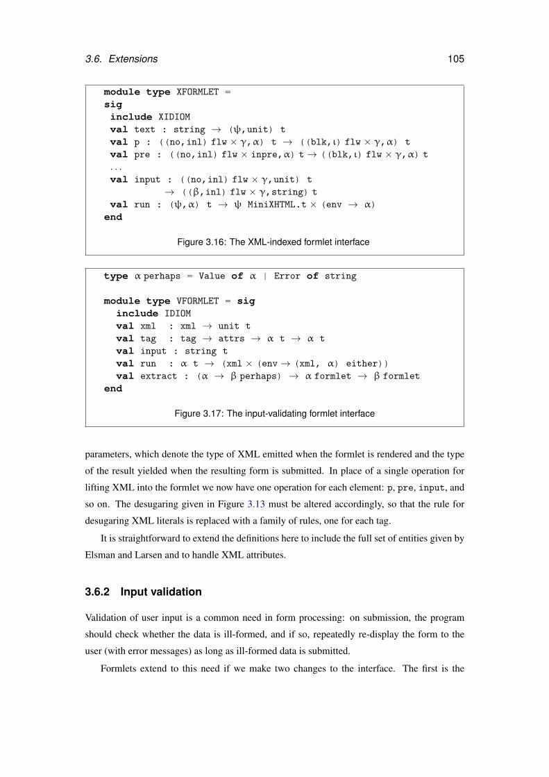
3.6. Extensions 105
module type XFORMLET =siginclude XIDIOM
val text : string → (ψ,unit) t
val p : ((no,inl) flw × γ,α) t → ((blk,ι) flw × γ,α) t
val pre : ((no,inl) flw × inpre,α) t→ ((blk,ι) flw × γ,α) t
. . .val input : ((no,inl) flw × γ,unit) t
→ ((β,inl) flw × γ,string) t
val run : (ψ,α) t → ψ MiniXHTML.t × (env → α)end
Figure 3.16: The XML-indexed formlet interface
type α perhaps = Value of α | Error of string
module type VFORMLET = siginclude IDIOM
val xml : xml → unit t
val tag : tag → attrs → α t → α t
val input : string t
val run : α t → (xml × (env→ (xml, α) either))val extract : (α → β perhaps) → α formlet → β formlet
end
Figure 3.17: The input-validating formlet interface
parameters, which denote the type of XML emitted when the formlet is rendered and the type
of the result yielded when the resulting form is submitted. In place of a single operation for
lifting XML into the formlet we now have one operation for each element: p, pre, input, and
so on. The desugaring given in Figure 3.13 must be altered accordingly, so that the rule for
desugaring XML literals is replaced with a family of rules, one for each tag.
It is straightforward to extend the definitions here to include the full set of entities given by
Elsman and Larsen and to handle XML attributes.
3.6.2 Input validation
Validation of user input is a common need in form processing: on submission, the program
should check whether the data is ill-formed, and if so, repeatedly re-display the form to the
user (with error messages) as long as ill-formed data is submitted.
Formlets extend to this need if we make two changes to the interface. The first is the
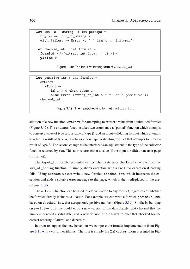
106 Chapter 3. Abstracting controls
let int (s : string) : int perhaps =try Value (int_of_string s)with Failure → Error (s ^ " isn’t an integer")
let checked_int : int formlet =formlet <#>{extract int input ⇒ v}</#>yields v
Figure 3.18: The input-validating formlet checked_int.
let positive_int : int formlet =extract
(fun i→if i > 0 then Value i
else Error (string_of_int s ^ " isn’t positive"))checked_int
Figure 3.19: The input-checking formlet positive_int.
addition of a new function, extract, for attempting to extract a value from a submitted formlet
(Figure 3.17). The extract function takes two arguments: a “partial” function which attempts
to convert a value of type α to a value of type β, and an input-validating formlet which attempts
to return a result of type α; it returns a new input-validating formlet that attempts to return a
result of type β. The second change to the interface is an adjustment to the type of the collector
function returned by run. This now returns either a value (if the input is valid) or an error page
(if it is not).
The input_int formlet presented earlier inherits its error checking behaviour from the
int_of_string function: it simply aborts execution with a Failure exception if parsing
fails. Using extract we can write a new formlet, checked_int, which intercepts the ex-
ception and adds a suitable error message to the page, which is then redisplayed to the user
(Figure 3.18).
The extract function can be used to add validation to any formlet, regardless of whether
the formlet already includes validation. For example, we can write a formlet, positive_int,
based on checked_int, that accepts only positive numbers (Figure 3.19). Similarly, building
on positive_int, we could write a new version of the date formlet that checked that the
numbers denoted a valid date, and a new version of the travel formlet that checked for the
correct ordering of arrival and departure.
In order to support the new behaviour we compose the formlet implementation from Fig-
ure 3.11 with two further idioms. The first is simply the XmlWriter idiom presented in Fig-
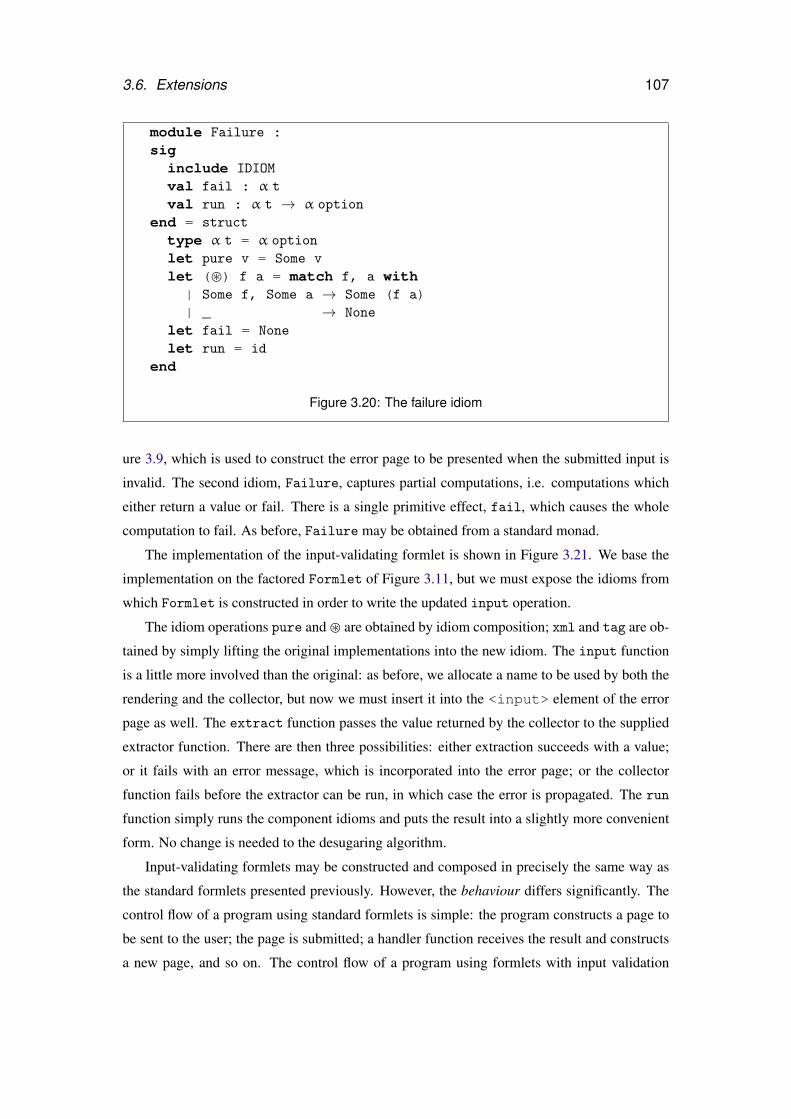
3.6. Extensions 107
module Failure :siginclude IDIOM
val fail : α t
val run : α t → α option
end = struct
type α t = α option
let pure v = Some v
let (�) f a = match f, a with| Some f, Some a → Some (f a)| _ → None
let fail = None
let run = id
end
Figure 3.20: The failure idiom
ure 3.9, which is used to construct the error page to be presented when the submitted input is
invalid. The second idiom, Failure, captures partial computations, i.e. computations which
either return a value or fail. There is a single primitive effect, fail, which causes the whole
computation to fail. As before, Failure may be obtained from a standard monad.
The implementation of the input-validating formlet is shown in Figure 3.21. We base the
implementation on the factored Formlet of Figure 3.11, but we must expose the idioms from
which Formlet is constructed in order to write the updated input operation.
The idiom operations pure and � are obtained by idiom composition; xml and tag are ob-
tained by simply lifting the original implementations into the new idiom. The input function
is a little more involved than the original: as before, we allocate a name to be used by both the
rendering and the collector, but now we must insert it into the <input> element of the error
page as well. The extract function passes the value returned by the collector to the supplied
extractor function. There are then three possibilities: either extraction succeeds with a value;
or it fails with an error message, which is incorporated into the error page; or the collector
function fails before the extractor can be run, in which case the error is propagated. The run
function simply runs the component idioms and puts the result into a slightly more convenient
form. No change is needed to the desugaring algorithm.
Input-validating formlets may be constructed and composed in precisely the same way as
the standard formlets presented previously. However, the behaviour differs significantly. The
control flow of a program using standard formlets is simple: the program constructs a page to
be sent to the user; the page is submitted; a handler function receives the result and constructs
a new page, and so on. The control flow of a program using formlets with input validation
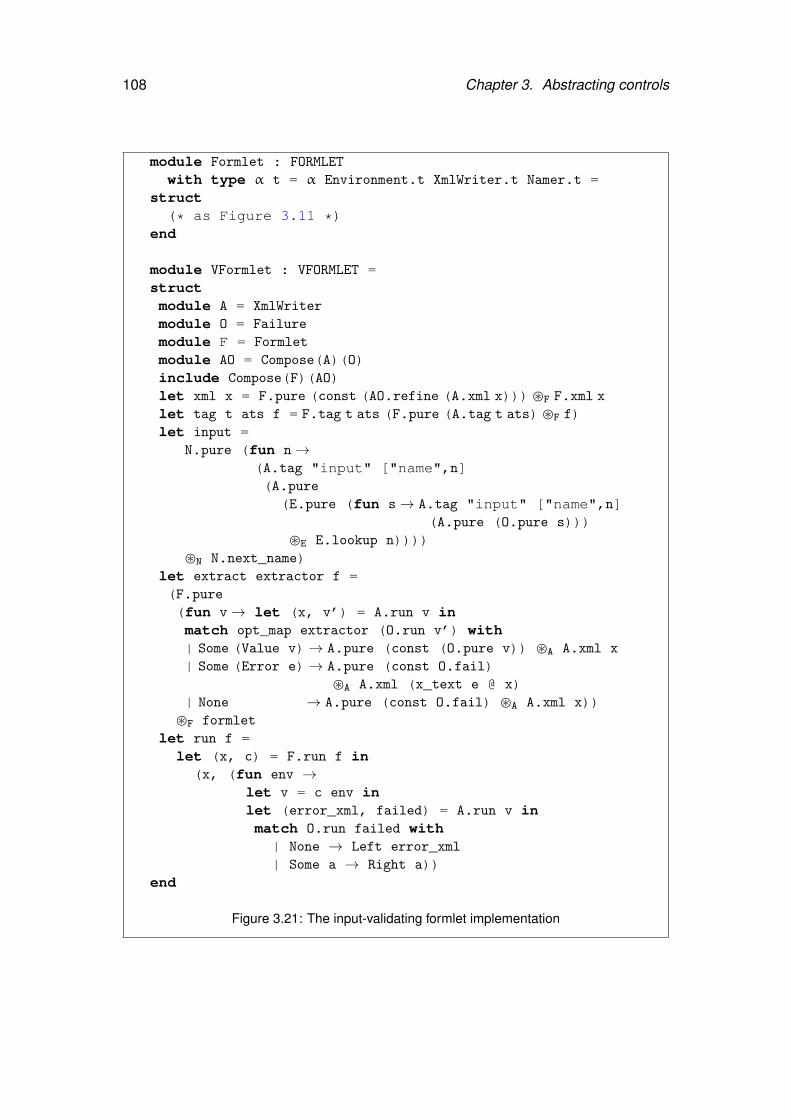
108 Chapter 3. Abstracting controls
module Formlet : FORMLET
with type α t = α Environment.t XmlWriter.t Namer.t =struct
(* as Figure 3.11 *)end
module VFormlet : VFORMLET =structmodule A = XmlWriter
module O = Failure
module F = Formlet
module AO = Compose(A)(O)include Compose(F)(AO)let xml x = F.pure (const (AO.refine (A.xml x))) �F F.xml x
let tag t ats f = F.tag t ats (F.pure (A.tag t ats) �F f)let input =
N.pure (fun n→(A.tag "input" ["name",n](A.pure
(E.pure (fun s→ A.tag "input" ["name",n](A.pure (O.pure s)))
�E E.lookup n))))�N N.next_name)
let extract extractor f =(F.pure(fun v→ let (x, v’) = A.run v inmatch opt_map extractor (O.run v’) with| Some (Value v)→ A.pure (const (O.pure v)) �A A.xml x
| Some (Error e)→ A.pure (const O.fail)�A A.xml (x_text e @ x)
| None → A.pure (const O.fail) �A A.xml x))�F formlet
let run f =let (x, c) = F.run f in
(x, (fun env →let v = c env inlet (error_xml, failed) = A.run v inmatch O.run failed with
| None → Left error_xml| Some a → Right a))
end
Figure 3.21: The input-validating formlet implementation
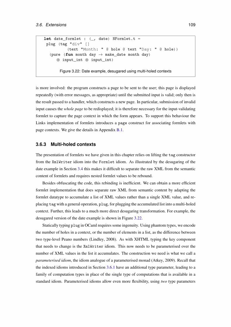
3.6. Extensions 109
let date_formlet : (_, date) NFormlet.t =plug (tag "div" []
(text "Month: " @ hole @ text "Day: " @ hole))(pure (fun month day → make_date month day)
� input_int � input_int)
Figure 3.22: Date example, desugared using multi-holed contexts
is more involved: the program constructs a page to be sent to the user; this page is displayed
repeatedly (with error messages, as appropriate) until the submitted input is valid; only then is
the result passed to a handler, which constructs a new page. In particular, submission of invalid
input causes the whole page to be redisplayed; it is therefore necessary for the input-validating
formlet to capture the page context in which the form appears. To support this behaviour the
Links implementation of formlets introduces a page construct for associating formlets with
page contexts. We give the details in Appendix B.1.
3.6.3 Multi-holed contexts
The presentation of formlets we have given in this chapter relies on lifting the tag constructor
from the XmlWriter idiom into the Formlet idiom. As illustrated by the desugaring of the
date example in Section 3.4 this makes it difficult to separate the raw XML from the semantic
content of formlets and requires nested formlet values to be rebound.
Besides obfuscating the code, this rebinding is inefficient. We can obtain a more efficient
formlet implementation that does separate raw XML from semantic content by adapting the
formlet datatype to accumulate a list of XML values rather than a single XML value, and re-
placing tagwith a general operation, plug, for plugging the accumulated list into a multi-holed
context. Further, this leads to a much more direct desugaring transformation. For example, the
desugared version of the date example is shown in Figure 3.22.
Statically typing plug in OCaml requires some ingenuity. Using phantom types, we encode
the number of holes in a context, or the number of elements in a list, as the difference between
two type-level Peano numbers (Lindley, 2008). As with XHTML typing the key component
that needs to change is the XmlWriter idiom. This now needs to be parameterised over the
number of XML values in the list it accumulates. The construction we need is what we call a
parameterised idiom, the idiom analogue of a parameterised monad (Atkey, 2009). Recall that
the indexed idioms introduced in Section 3.6.1 have an additional type parameter, leading to a
family of computation types in place of the single type of computations that is available in a
standard idiom. Parameterised idioms allow even more flexibility, using two type parameters
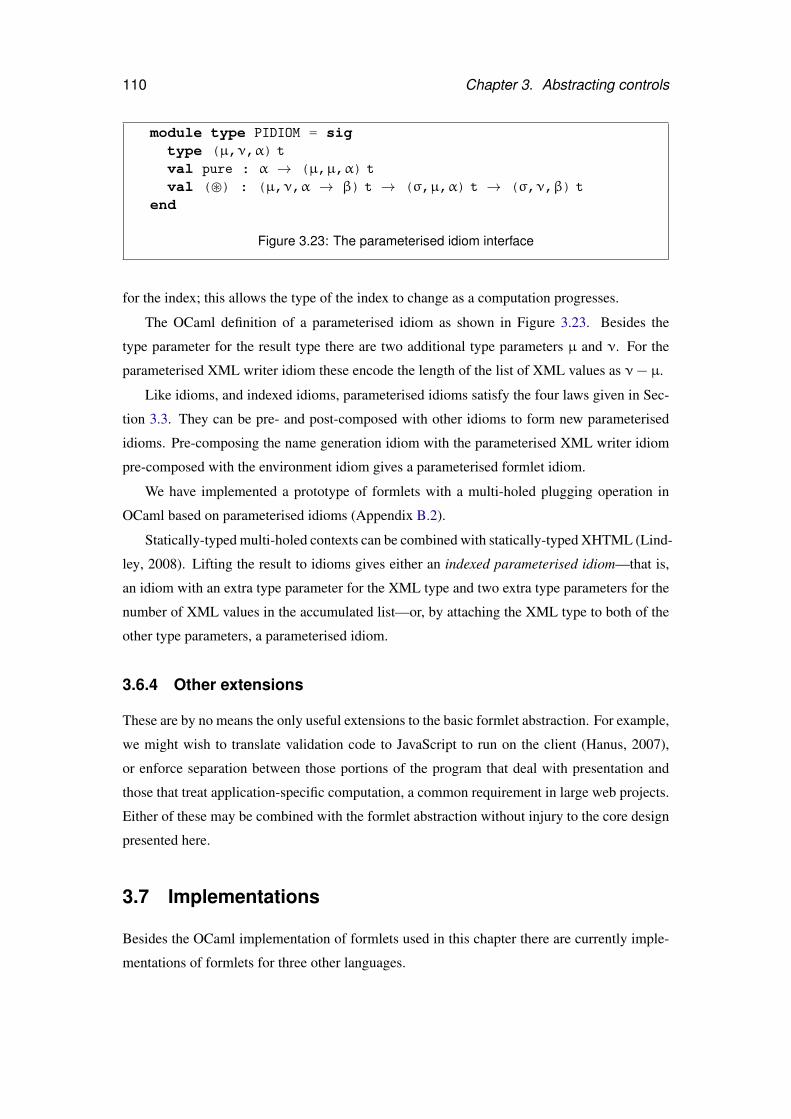
110 Chapter 3. Abstracting controls
module type PIDIOM = sigtype (µ,ν,α) t
val pure : α → (µ,µ,α) t
val (�) : (µ,ν,α → β) t → (σ,µ,α) t → (σ,ν,β) t
end
Figure 3.23: The parameterised idiom interface
for the index; this allows the type of the index to change as a computation progresses.
The OCaml definition of a parameterised idiom as shown in Figure 3.23. Besides the
type parameter for the result type there are two additional type parameters µ and ν. For the
parameterised XML writer idiom these encode the length of the list of XML values as ν− µ.
Like idioms, and indexed idioms, parameterised idioms satisfy the four laws given in Sec-
tion 3.3. They can be pre- and post-composed with other idioms to form new parameterised
idioms. Pre-composing the name generation idiom with the parameterised XML writer idiom
pre-composed with the environment idiom gives a parameterised formlet idiom.
We have implemented a prototype of formlets with a multi-holed plugging operation in
OCaml based on parameterised idioms (Appendix B.2).
Statically-typed multi-holed contexts can be combined with statically-typed XHTML (Lind-
ley, 2008). Lifting the result to idioms gives either an indexed parameterised idiom—that is,
an idiom with an extra type parameter for the XML type and two extra type parameters for the
number of XML values in the accumulated list—or, by attaching the XML type to both of the
other type parameters, a parameterised idiom.
3.6.4 Other extensions
These are by no means the only useful extensions to the basic formlet abstraction. For example,
we might wish to translate validation code to JavaScript to run on the client (Hanus, 2007),
or enforce separation between those portions of the program that deal with presentation and
those that treat application-specific computation, a common requirement in large web projects.
Either of these may be combined with the formlet abstraction without injury to the core design
presented here.
3.7 Implementations
Besides the OCaml implementation of formlets used in this chapter there are currently imple-
mentations of formlets for three other languages.
3.8. Related work 111
Formlets were initially implemented in Links (Cooper et al., 2008b), which provides the
syntax presented here. The Links implementation includes many features, such as a full suite
of HTML controls (textareas, pop-up menus, radio buttons, etc.), which are not described here.
Strugnell has ported a commercial web-based project-management application originally im-
plemented in PHP to the Links version of formlets (Strugnell, 2008). He gives an in-depth
comparison between Links formlets and forms implemented in PHP.
Eidhof has released a Haskell implementation of formlets (Eidhof, 2008), based on the de-
scription in Cooper et al. (2008b). The current revision contains a number of useful extensions.
For example, validation functions include support for monadic actions, making it possible to
perform IO (such as reading from a database) while checking the validity of user input.
McCarthy has added formlets to PLT Scheme based on the description in Cooper et al.
(2008a); they are available from version 4.1.1 onwards. Support for a variant of the formlet
syntax is provided using macros.
3.8 Related work
The WASH, iData and WUI frameworks all support aspects of the form abstraction we have
presented. Underlying all these systems is the essential mode of form abstraction we describe,
although they vary significantly in their feature sets and limitations.
WASH The WASH/CGI Haskell framework (Thiemann, 2005) supports a variety of web
application needs, including forms with some abstraction. WASH supports user-defined types
as the result of an individual form field, through defining a Read instance, which parses the
type from a string. It also supports aggregating data from multiple fields using a suite of tupling
constructors, but it does not allow arbitrary calculations from these multiple fields into other
data types, such as our abstract date type. In particular, the tupling constructors still expose
the structure of the form fields, preventing true abstraction. For example, given a one-field
component, a programmer cannot modify it to consist of two fields without also changing all
the uses of the component.
iData The iData framework (Plasmeijer and Achten, 2006) supports a high degree of form
abstraction, calling its abstractions iData. Underlying iData is an abstraction much like form-
lets. Unlike formlets, where form abstraction is separated from control flow (the function
handle attaches a handler to a formlet), iData integrate control flow and form composition into
a single abstraction. An iData program defines a single web page consisting of a collection of
interdependent iData. Whenever a form element is edited by the user, the form is submitted and
112 Chapter 3. Abstracting controls
then re-displayed to the user with any dependencies resolved. The iTasks library (Plasmeijer,
Achten, and Koopman, 2007) builds on top of iData by enabling or disabling iData according
to the state of the program.
WUI The WUI (Web User Interface) library (Hanus, 2006, 2007) implements form abstrac-
tions for the functional logic programming language Curry. The basic units are called WUIs,
defined by the type WuiSpec. Like iData, WUIs are designed around the idea of editing; the
WUI library provides particular support for presenting application data to the user for modifi-
cation. Consequently, each WUI of type WuiSpec α both consumes and generates a value of
type α; the consumed value models the default or current value for the component. WUIs are
similar in spirit to formlets: there is a library of basic WUIs for primitive types and a set of
combinators for constructing WUIs for user-defined types, such as transformWSpec, which
is an analogue of the mapFormlet function definable in the formlet idiom:
transformWSpec :: (α→ β,β→ α) → WuiSpec α → WuiSpec β
val mapFormlet : (α→ β) → α formlet → β formlet
let mapFormlet g f = formlet <#>{f ⇒ x}</#> yields g x
WUIs also support user-input validation through an interface that is similar to our extension of
formlets in Section 3.6.2 .
WUIs cannot be characterised as idioms, due to the negative occurrence of the type pa-
rameter in the definition of WuiSpec; for the same reason, it appears that WUIs cannot strictly
implement formlets. However, formlets can implement WUIs: a WUI is equivalent to a value
of type α→ α formlet.
The implementation of WUIs is rather different from the approach presented here. Whereas
formlets are based on functional abstraction (and so can be adapted to any functional program-
ming language), the WUI library takes advantage of the distinctive features of Curry; for exam-
ple, it uses logic variables to generate the equivalent of fresh names for input fields, avoiding
the need to use a monad or idiom to generate fresh names, as with formlets.
3.9 Conclusions
We have described formlets, a construct for composable HTML form fragments that capture the
essence of form abstraction. We have argued that formlets are best modelled as idioms (rather
than monads or arrows), and shown how to extend the core abstraction in several orthogonal
directions, such as static validation of generated XHTML and dynamic validation of user-
input, while remaining within the idiom framework. Formlets can be implemented within any
3.9. Conclusions 113
functional language, and there are currently formlet libraries for Haskell, OCaml, Links and
PLT Scheme. The latter three implementations also support the syntactic sugar described here,
which makes formlets more pleasant to use in practice.

Chapter 4
Serialising continuations1
4.1 Introduction
The Formlet library described in Chapter 3 depends on a small number of primitive functions.
One of these primitives, pickle_cont, serialises a function into an externalisable represen-
tation which can be sent to a client. Links functions are represented as values of OCaml, the
host language for the Links prototype implementation; serialising a Links function involves
converting between its OCaml representation and a string encoding the same structure. This
chapter describes the approach to serialisation used in the Links implementation.
4.1.1 Requirements
We apply several criteria in the search for a suitable approach to serialisation for Links.
1. Efficiency. Space efficiency is of primary importance to keep network traffic low and
avoid imposing too great a burden on clients.
2. Type-safety. Applying a deserialisation function to invalid data should never cause a
program crash.
3. Extensibility. Most of the time an out-of-the-box serialiser is sufficient, but there is
sometimes a need for a user to supply a specialised implementation of serialisation at a
particular type.
4. Maintainability. A solution which requires the user to write and maintain large amounts
of code to perform basic serialisation is not acceptable.
1This chapter is a revision of Yallop (2007)
115
116 Chapter 4. Serialising continuations
We must emphasise that these are the requirements for the Links prototype, not for seri-
alisation in general. Other systems may well require further properties, such as adherence to
an externally-specified format (such as ASN.1), forwards and backward compatibility, and so
on. We also choose not to address security considerations (notably maintaining the secrecy and
integrity of serialised data) in what follows, taking the view that these may be addressed ex-
ternally, for example by encrypting serialised functions before passing them to the client (Bal-
topoulos and Gordon, 2009).
4.1.2 Existing approaches
We will first consider two existing approaches to serialisation: the standard OCaml module
Marshal, and pickler combinators.
4.1.2.1 Marshal
The OCaml standard library includes a module, Marshal, with functions
val to_string : ∀α.α → extern_flags list → string
val from_string : ∀α.string → int → α
that allow almost any value to be serialised and reconstructed. While Marshal is certainly
easy to use, its design is problematic when judged for flexibility and safety. The encoding of
values is unspecified and fixed, leaving no way to specialise the encoding at a particular type.
The type of the to_string function places no restrictions on its input, delaying detection of
attempts to serialise unserialisable values until runtime.
# Marshal.to_string (lazy 0) [];;Exception: Invalid_argument
"output_value: abstract value (outside heap)".
Most seriously of all, it is easy to use Marshal to write programs that crash by interpreting a
reconstructed value at a wrong type.
# (Marshal.from_string (Marshal.to_string 0 []) 0 : float);;Segmentation fault
These flaws make Marshal most suitable for use as a basis for a safe implementation that
includes some independent means of verifying the integrity and suitability of marshalled data.
4.1.2.2 Pickler combinators
Compositionality is perhaps the greatest benefit of functional programming (Hughes, 1989), so
it is natural to seek a combinator approach to the serialisation problem. There is a natural way to
4.1. Introduction 117
structure a combinator library for serialisation, as evinced by the similarity of proposed designs
by Kennedy (2004) for Haskell and Elsman (2005) for SML. Starting with a parameterised type
of serialisers
type α pu
together with serialisers for primitive types
val int : int pu
val unit : unit pu
val bool : bool pu
and combinators for parameterised types that take serialisers to serialisers
val list : ∀α.α pu → α list pu
val pair : ∀α,β.(α pu) × (β pu) → (α × β) pu
and a function which takes conversions between types to conversions between serialisers
val wrap : ∀α,β.(α→ β) → (β→ α) → (α pu→ β pu)
we can encode a wide variety of datatypes. To serialise user-defined algebraic types we need
some way of discriminating between the constructors. The typical solution is to provide a
combinator (called data in Elsman (2005), alt in Kennedy (2004)) whose argument maps
constructors to integers:
val alt : ∀α.(α → int) → α pu list → α pu
We might then write a pu for OCaml’s option type as follows:
let option : ∀α.α pu → α option pu =fun a →
alt
(function None → 0 | (Some _) → 1)[wrap (fun () → None) (fun None → ()) unit;wrap (fun v → Some v) (fun (Some v) → v) a];
The combinator approach has none of the problems seen with Marshal: the user can choose
the encoding at each type, and there is no lack of type-safety. There are, however, serious
drawbacks particular to this approach. First, it requires recapitulating the structure of each
user-defined type to obtain a serialiser: this is a prime example of the “boilerplate” which
much recent research has sought ways to “scrap” (Lämmel and Peyton Jones, 2003). Secondly,
the requirement for the user to supply a mapping from constructors to integers can lead to errors
that are hard to track down. Finally, there are difficulties in handling both cyclic values, which
can arise in ML through the use of references, and mutually recursive datatypes. The refCyc
combinator described by Elsman (2005) supports cyclic values, but requires the user to supply
a “dummy” value to start off the cycle:
118 Chapter 4. Serialising continuations
val refCyc : ∀α.α → α pu → α ref pu
Not only is this a rather unpleasant imposition, but it is not apparent whether it can be readily
generalised to the OCaml situation, where mutability is introduced not by the ref type, but
by records with arbitrary numbers of mutable fields. Karvonen (2007) notes that the need
for a dummy value can be eliminated by using an additional generic function that constructs
witnesses for types.
4.2 Generic functions
The operations provided by pickler combinators are examples of generic functions. Generic
functions are based on a form of polymorphism which lies between the extremes of parametric
and ad-hoc. The behaviour of a parametrically polymorphic function, such as length, is the
same at every type. The behaviour of an ad-hoc polymorphic function, such as sum, is different
at each type at which it is defined. The behaviour of a generic function, such as pickle or eq,
also varies at each type, but in a way that is related to the type structure.
Put another way, parametric polymorphic functions are parameterised by type, ad-hoc poly-
morphic functions by instance, and generic functions by the shape of types. For example, eq
is defined in the same way for every (immutable) record type: two values of a record type are
equal if the values of corresponding fields are equal. The definition of eq varies with the shape
of its argument type: in the case of records it is a function of the set of fields in the type.
The definition of a generic function at a particular type typically follows the definition of
the type exactly. There is therefore no real reason to require a programmer to write out the
definitions of such functions for each new type he defines. The Haskell definition specifies a
means by which a programmer can request the implementation to derive suitable definitions
automatically (for a fixed set of standard type classes) (Peyton Jones and Hughes, 1999). In the
following pages we describe an analogous facility for OCaml, which relieves the programmer
of the need to write out serialisation functions when defining new types. Like Haskell’s facility,
our system can be applied to any suitable type. However, the Links prototype only needs to
apply it at a fixed set of types, namely those types which are used to represent Links syntax and
Links values within the OCaml code that forms the Links implementation.
4.2.1 Example: generic equality
We begin with a simple example. Figure 4.1 gives the definitions of two datatypes which
support equality. The code is all standard OCaml, except for the clause
deriving (Eq)
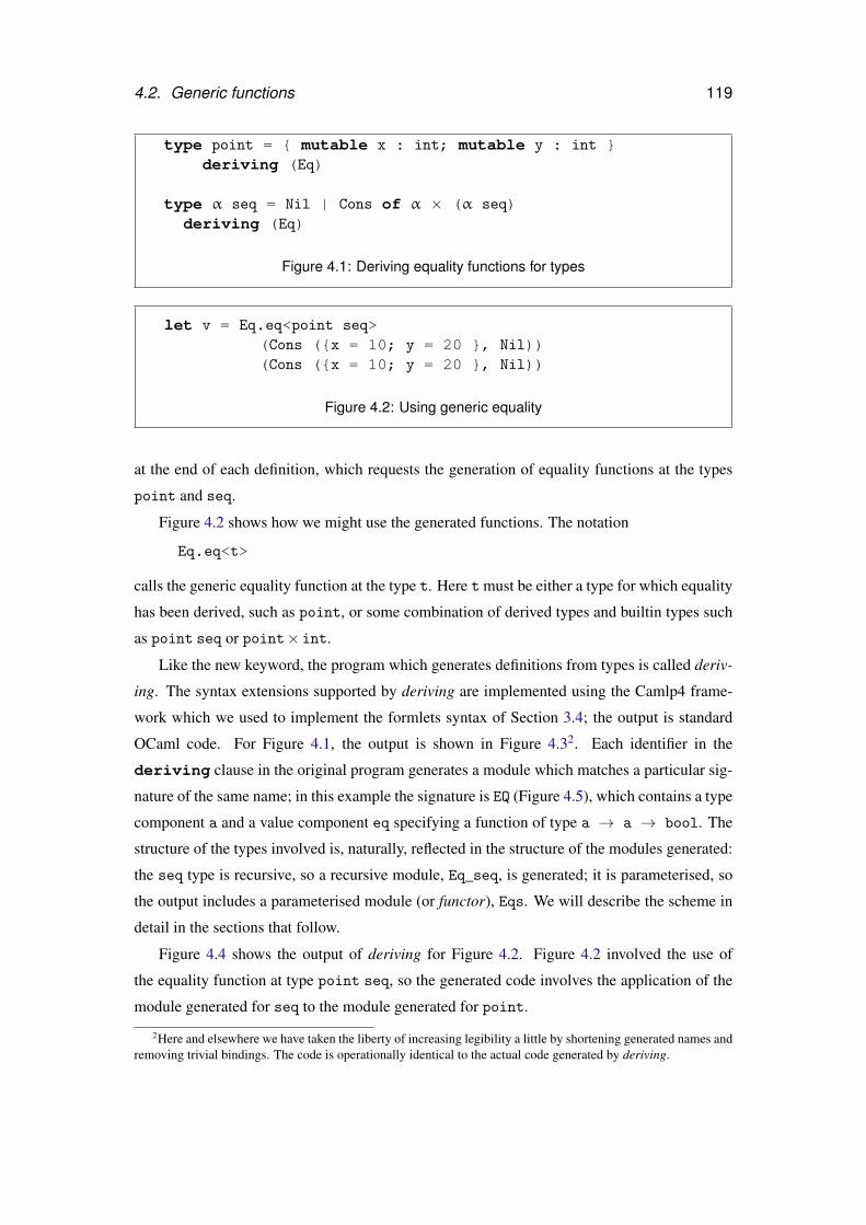
4.2. Generic functions 119
type point = { mutable x : int; mutable y : int }deriving (Eq)
type α seq = Nil | Cons of α × (α seq)deriving (Eq)
Figure 4.1: Deriving equality functions for types
let v = Eq.eq<point seq>(Cons ({x = 10; y = 20 }, Nil))(Cons ({x = 10; y = 20 }, Nil))
Figure 4.2: Using generic equality
at the end of each definition, which requests the generation of equality functions at the types
point and seq.
Figure 4.2 shows how we might use the generated functions. The notation
Eq.eq<t>
calls the generic equality function at the type t. Here t must be either a type for which equality
has been derived, such as point, or some combination of derived types and builtin types such
as point seq or point× int.
Like the new keyword, the program which generates definitions from types is called deriv-
ing. The syntax extensions supported by deriving are implemented using the Camlp4 frame-
work which we used to implement the formlets syntax of Section 3.4; the output is standard
OCaml code. For Figure 4.1, the output is shown in Figure 4.32. Each identifier in the
deriving clause in the original program generates a module which matches a particular sig-
nature of the same name; in this example the signature is EQ (Figure 4.5), which contains a type
component a and a value component eq specifying a function of type a → a → bool. The
structure of the types involved is, naturally, reflected in the structure of the modules generated:
the seq type is recursive, so a recursive module, Eq_seq, is generated; it is parameterised, so
the output includes a parameterised module (or functor), Eqs. We will describe the scheme in
detail in the sections that follow.
Figure 4.4 shows the output of deriving for Figure 4.2. Figure 4.2 involved the use of
the equality function at type point seq, so the generated code involves the application of the
module generated for seq to the module generated for point.
2Here and elsewhere we have taken the liberty of increasing legibility a little by shortening generated names andremoving trivial bindings. The code is operationally identical to the actual code generated by deriving.
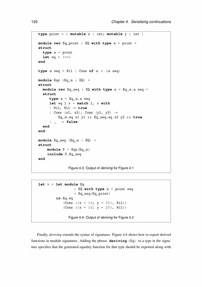
120 Chapter 4. Serialising continuations
type point = { mutable x : int; mutable y : int }
module rec Eq_point : EQ with type a = point =struct
type a = point
let eq = (==)end
type α seq = Nil | Cons of α × (α seq)
module Eqs (Eq_α : EQ) =struct
module rec Eq_seq : EQ with type a = Eq_α.a seq =struct
type a = Eq_α.a seq
let eq l r = match l, r with| Nil, Nil → true| Cons (x1, x2), Cons (y1, y2) →
Eq_α.eq x1 y1 && Eq_seq.eq x2 y2 && true| _ → false
endend
module Eq_seq (Eq_α : EQ) =struct
module P = Eqs(Eq_α)include P.Eq_seq
end
Figure 4.3: Output of deriving for Figure 4.1
let v = let module Eq
: EQ with type a = point seq
= Eq_seq(Eq_point)in Eq.eq
(Cons ({x = 10; y = 20}, Nil))(Cons ({x = 10; y = 20}, Nil))
Figure 4.4: Output of deriving for Figure 4.2
Finally, deriving extends the syntax of signatures. Figure 4.6 shows how to export derived
functions in module signatures. Adding the phrase deriving (Eq) to a type in the signa-
ture specifies that the generated equality function for that type should be exported along with
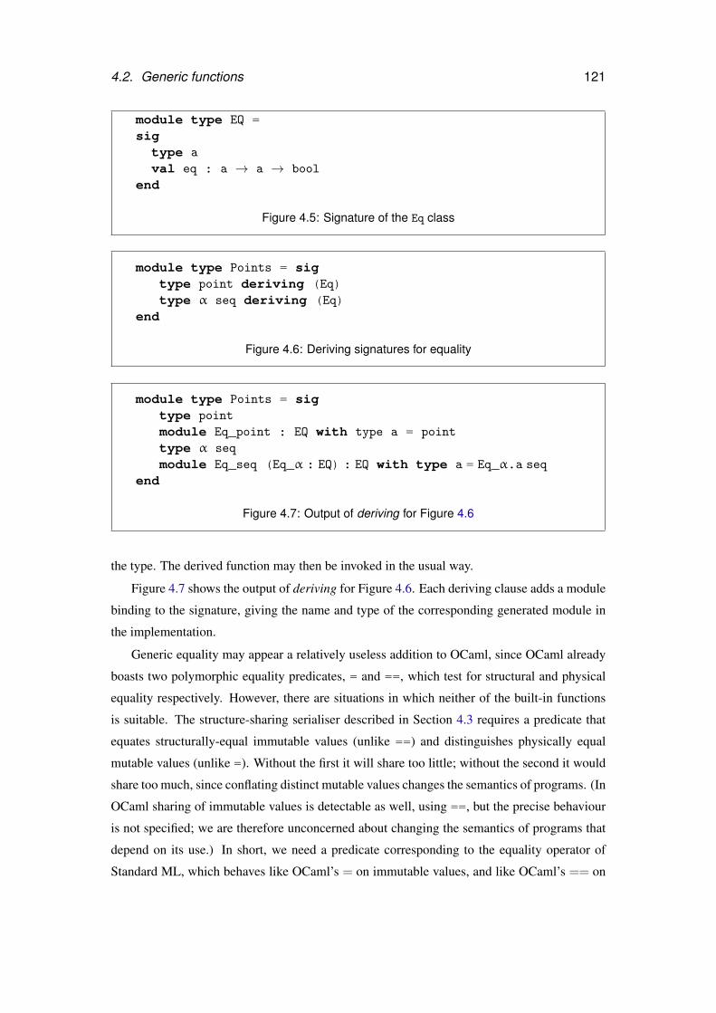
4.2. Generic functions 121
module type EQ =sig
type a
val eq : a → a → bool
end
Figure 4.5: Signature of the Eq class
module type Points = sigtype point deriving (Eq)type α seq deriving (Eq)
end
Figure 4.6: Deriving signatures for equality
module type Points = sigtype point
module Eq_point : EQ with type a = point
type α seq
module Eq_seq (Eq_α : EQ) : EQ with type a = Eq_α.a seq
end
Figure 4.7: Output of deriving for Figure 4.6
the type. The derived function may then be invoked in the usual way.
Figure 4.7 shows the output of deriving for Figure 4.6. Each deriving clause adds a module
binding to the signature, giving the name and type of the corresponding generated module in
the implementation.
Generic equality may appear a relatively useless addition to OCaml, since OCaml already
boasts two polymorphic equality predicates, = and ==, which test for structural and physical
equality respectively. However, there are situations in which neither of the built-in functions
is suitable. The structure-sharing serialiser described in Section 4.3 requires a predicate that
equates structurally-equal immutable values (unlike ==) and distinguishes physically equal
mutable values (unlike =). Without the first it will share too little; without the second it would
share too much, since conflating distinct mutable values changes the semantics of programs. (In
OCaml sharing of immutable values is detectable as well, using ==, but the precise behaviour
is not specified; we are therefore unconcerned about changing the semantics of programs that
depend on its use.) In short, we need a predicate corresponding to the equality operator of
Standard ML, which behaves like OCaml’s = on immutable values, and like OCaml’s == on
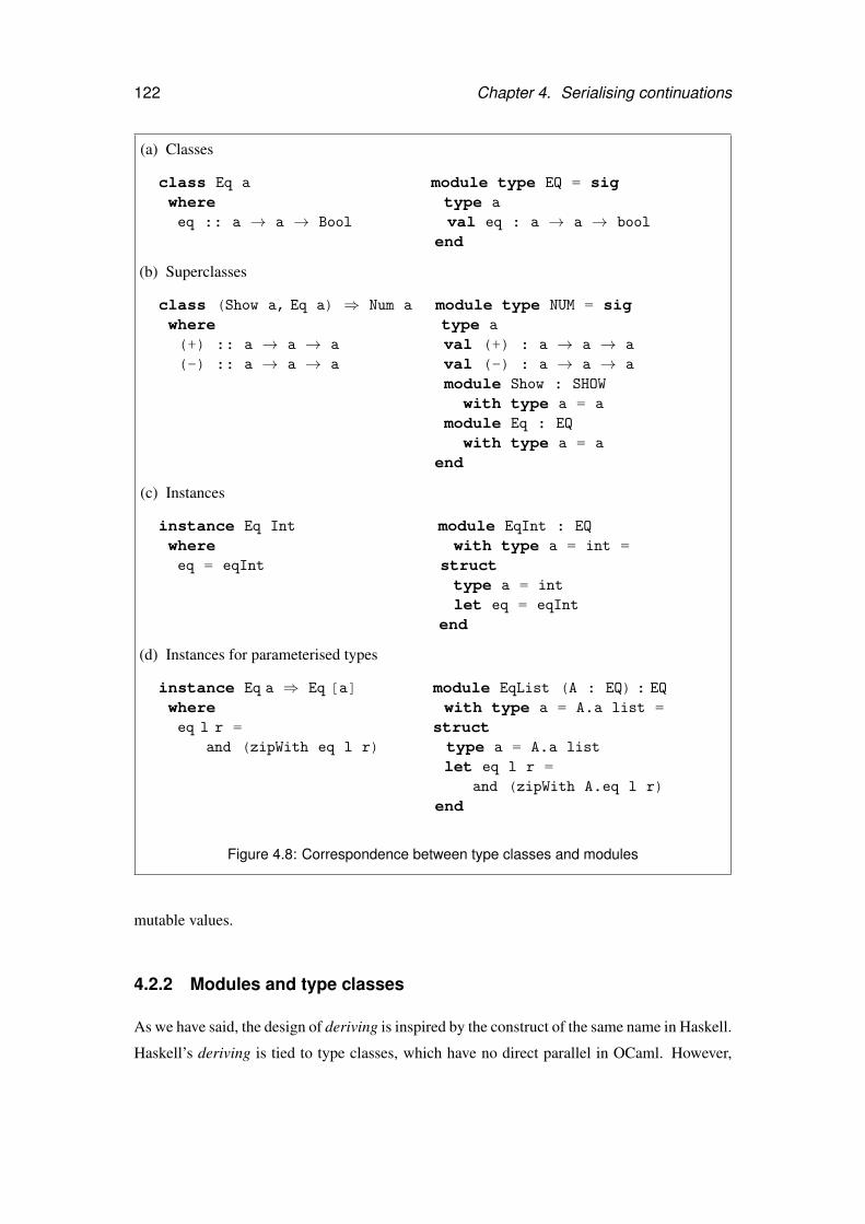
122 Chapter 4. Serialising continuations
(a) Classes
class Eq a module type EQ = sigwhere type a
eq :: a → a → Bool val eq : a → a → bool
end
(b) Superclasses
class (Show a, Eq a) ⇒ Num a module type NUM = sigwhere type a
(+) :: a → a → a val (+) : a → a → a
(-) :: a → a → a val (-) : a → a → a
module Show : SHOW
with type a = a
module Eq : EQ
with type a = a
end
(c) Instances
instance Eq Int module EqInt : EQ
where with type a = int =eq = eqInt struct
type a = int
let eq = eqInt
end
(d) Instances for parameterised types
instance Eq a ⇒ Eq [a] module EqList (A : EQ) : EQ
where with type a = A.a list =eq l r = struct
and (zipWith eq l r) type a = A.a list
let eq l r =and (zipWith A.eq l r)
end
Figure 4.8: Correspondence between type classes and modules
mutable values.
4.2.2 Modules and type classes
As we have said, the design of deriving is inspired by the construct of the same name in Haskell.
Haskell’s deriving is tied to type classes, which have no direct parallel in OCaml. However,
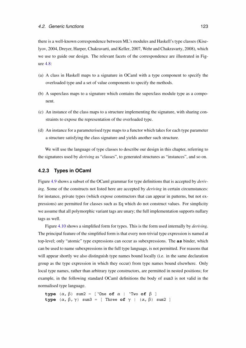
4.2. Generic functions 123
there is a well-known correspondence between ML’s modules and Haskell’s type classes (Kise-
lyov, 2004, Dreyer, Harper, Chakravarti, and Keller, 2007, Wehr and Chakravarty, 2008), which
we use to guide our design. The relevant facets of the correspondence are illustrated in Fig-
ure 4.8:
(a) A class in Haskell maps to a signature in OCaml with a type component to specify the
overloaded type and a set of value components to specify the methods.
(b) A superclass maps to a signature which contains the superclass module type as a compo-
nent.
(c) An instance of the class maps to a structure implementing the signature, with sharing con-
straints to expose the representation of the overloaded type.
(d) An instance for a parameterised type maps to a functor which takes for each type parameter
a structure satisfying the class signature and yields another such structure.
We will use the language of type classes to describe our design in this chapter, referring to
the signatures used by deriving as “classes”, to generated structures as “instances”, and so on.
4.2.3 Types in OCaml
Figure 4.9 shows a subset of the OCaml grammar for type definitions that is accepted by deriv-
ing. Some of the constructs not listed here are accepted by deriving in certain circumstances:
for instance, private types (which expose constructors that can appear in patterns, but not ex-
pressions) are permitted for classes such as Eq which do not construct values. For simplicity
we assume that all polymorphic variant tags are unary; the full implementation supports nullary
tags as well.
Figure 4.10 shows a simplified form for types. This is the form used internally by deriving.
The principal feature of the simplified form is that every non-trivial type expression is named at
top-level; only “atomic” type expressions can occur as subexpressions. The as binder, which
can be used to name subexpressions in the full type language, is not permitted. For reasons that
will appear shortly we also distinguish type names bound locally (i.e. in the same declaration
group as the type expression in which they occur) from type names bound elsewhere. Only
local type names, rather than arbitrary type constructors, are permitted in nested positions; for
example, in the following standard OCaml definitions the body of sum3 is not valid in the
normalised type language.
type (α,β) sum2 = [‘One of α | ‘Two of β ]type (α,β,γ) sum3 = [ Three of γ | (α,β) sum2 ]
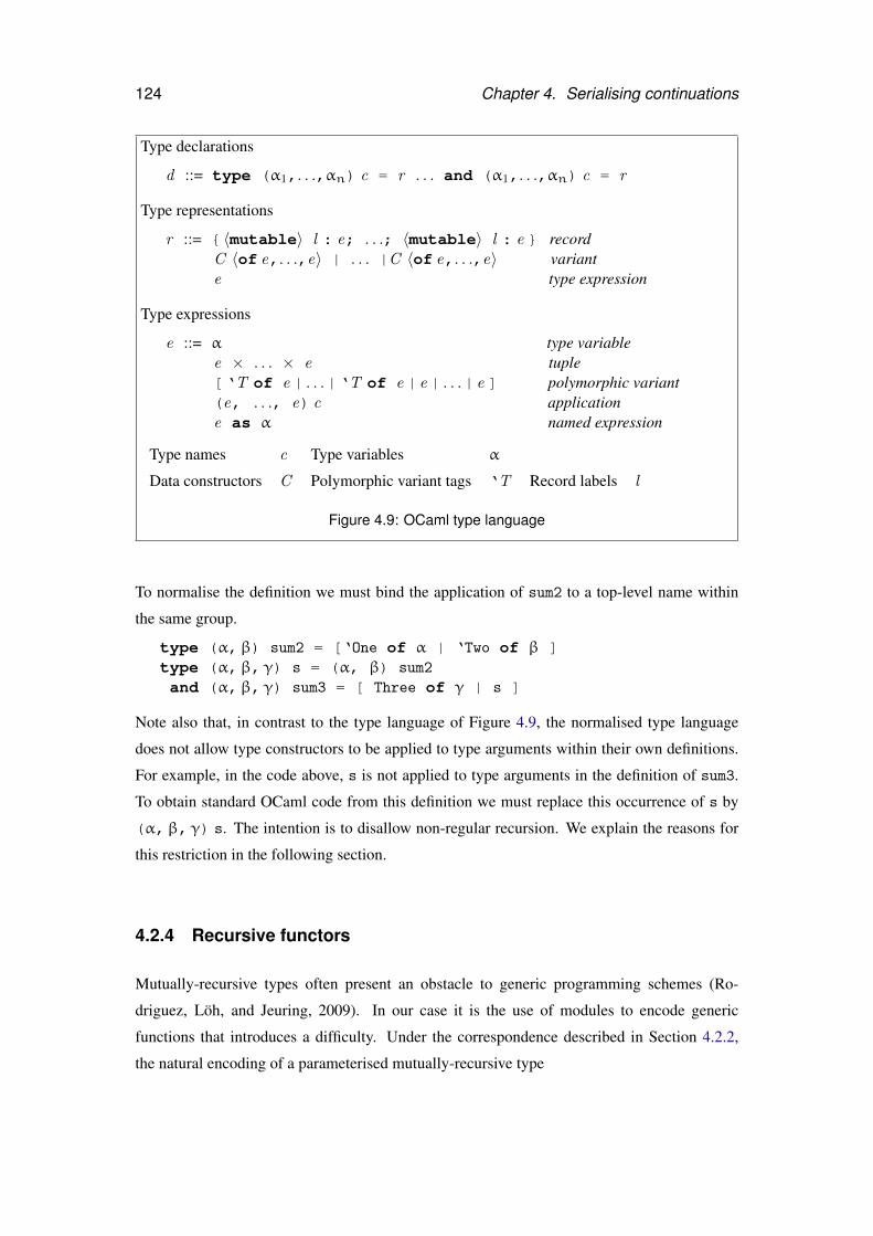
124 Chapter 4. Serialising continuations
Type declarations
d ::= type (α1,. . .,αn) c = r . . . and (α1,. . .,αn) c = r
Type representations
r ::= { 〈mutable〉 l : e; . . .; 〈mutable〉 l : e } recordC 〈of e,. . .,e〉 | . . . |C 〈of e,. . .,e〉 variante type expression
Type expressions
e ::= α type variablee × . . . × e tuple[‘T of e | . . .|‘T of e | e | . . .| e ] polymorphic variant(e, . . ., e) c applicatione as α named expression
Type names c Type variables α
Data constructors C Polymorphic variant tags ‘T Record labels l
Figure 4.9: OCaml type language
To normalise the definition we must bind the application of sum2 to a top-level name within
the same group.
type (α,β) sum2 = [‘One of α | ‘Two of β ]type (α,β,γ) s = (α, β) sum2
and (α,β,γ) sum3 = [ Three of γ | s ]
Note also that, in contrast to the type language of Figure 4.9, the normalised type language
does not allow type constructors to be applied to type arguments within their own definitions.
For example, in the code above, s is not applied to type arguments in the definition of sum3.
To obtain standard OCaml code from this definition we must replace this occurrence of s by
(α,β,γ) s. The intention is to disallow non-regular recursion. We explain the reasons for
this restriction in the following section.
4.2.4 Recursive functors
Mutually-recursive types often present an obstacle to generic programming schemes (Ro-
driguez, Löh, and Jeuring, 2009). In our case it is the use of modules to encode generic
functions that introduces a difficulty. Under the correspondence described in Section 4.2.2,
the natural encoding of a parameterised mutually-recursive type
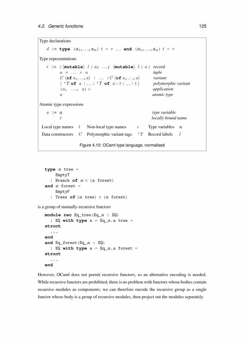
4.2. Generic functions 125
Type declarations
d ::= type (α1,. . .,αn) t = r . . . and (α1,. . .,αn) t = r
Type representations
r ::= { 〈mutable〉 l : a; . . .; 〈mutable〉 l : a } recorda × . . . × a tupleC 〈of a,. . .,a〉 | . . . |C 〈of a,. . .,a〉 variant[‘T of a | . . .|‘T of a | t | . . .| t ] polymorphic variant(a, . . ., a) c applicationa atomic type
Atomic type expressions
a ::= α type variablet locally bound name
Local type names t Non-local type names c Type variables α
Data constructors C Polymorphic variant tags ‘T Record labels l
Figure 4.10: OCaml type language, normalised
type α tree =EmptyT
| Branch of α × (α forest)and α forest =
EmptyF
| Trees of (α tree) × (α forest)
is a group of mutually-recursive functors
module rec Eq_tree(Eq_α : EQ): EQ with type a = Eq_α.a tree =
struct...
endand Eq_forest(Eq_α : EQ)
: EQ with type a = Eq_α.a forest =struct
...end
However, OCaml does not permit recursive functors, so an alternative encoding is needed.
While recursive functors are prohibited, there is no problem with functors whose bodies contain
recursive modules as components; we can therefore encode the recursive group as a single
functor whose body is a group of recursive modules, then project out the modules separately.
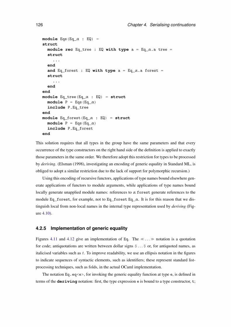
126 Chapter 4. Serialising continuations
module Eqs(Eq_α : EQ) =structmodule rec Eq_tree : EQ with type a = Eq_α.a tree =struct
...endand Eq_forest : EQ with type a = Eq_α.a forest =struct
...end
endmodule Eq_tree(Eq_α : EQ) = structmodule P = Eqs(Eq_α)include P.Eq_tree
endmodule Eq_forest(Eq_α : EQ) = struct
module P = Eqs(Eq_α)include P.Eq_forest
end
This solution requires that all types in the group have the same parameters and that every
occurrence of the type constructors on the right hand side of the definition is applied to exactly
those parameters in the same order. We therefore adopt this restriction for types to be processed
by deriving. (Elsman (1998), investigating an encoding of generic equality in Standard ML, is
obliged to adopt a similar restriction due to the lack of support for polymorphic recursion.)
Using this encoding of recursive functors, applications of type names bound elsewhere gen-
erate applications of functors to module arguments, while applications of type names bound
locally generate unapplied module names: references to α forest generate references to the
module Eq_forest, for example, not to Eq_forest Eq_α. It is for this reason that we dis-
tinguish local from non-local names in the internal type representation used by deriving (Fig-
ure 4.10).
4.2.5 Implementation of generic equality
Figures 4.11 and 4.12 give an implementation of Eq. The << . . .>> notation is a quotation
for code; antiquotations are written between dollar signs $ . . .$ or, for antiquoted names, as
italicised variables such as t . To improve readability, we use an ellipsis notation in the figures
to indicate sequences of syntactic elements, such as identifiers; these represent standard list-
processing techniques, such as folds, in the actual OCaml implementation.
The notation Eq.eq<e>, for invoking the generic equality function at type e, is defined in
terms of the deriving notation: first, the type expression e is bound to a type constructor, t;
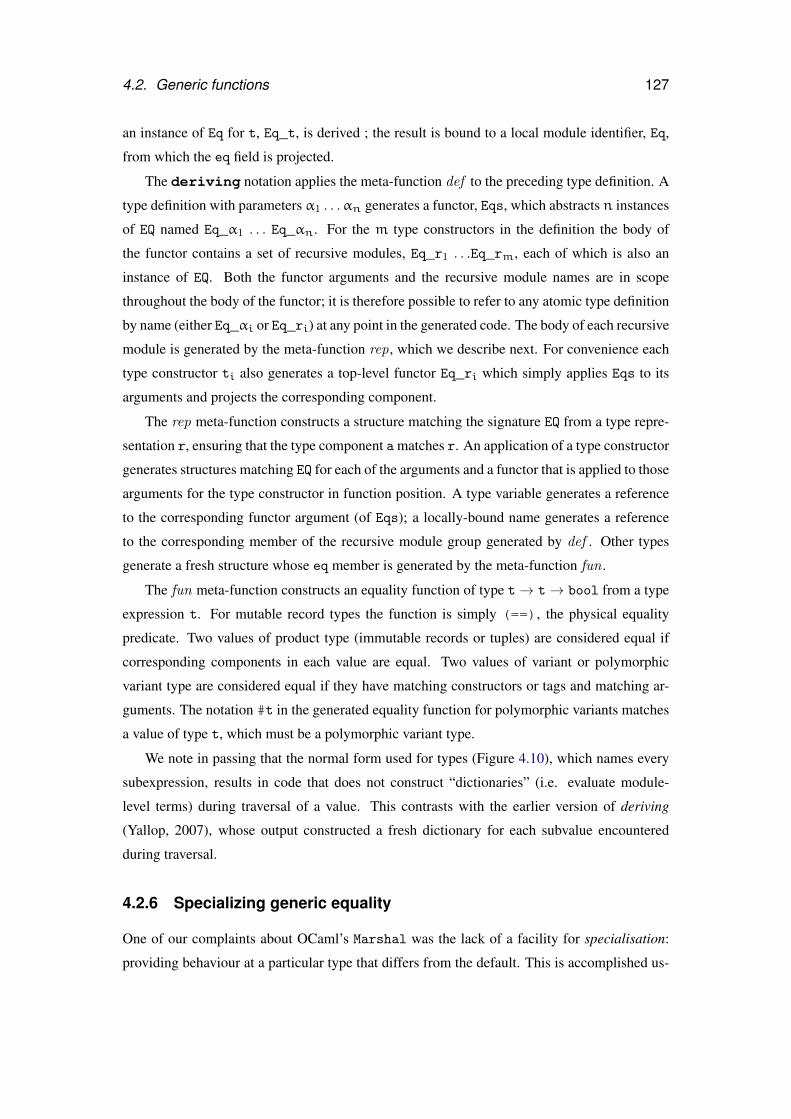
4.2. Generic functions 127
an instance of Eq for t, Eq_t, is derived ; the result is bound to a local module identifier, Eq,
from which the eq field is projected.
The deriving notation applies the meta-function def to the preceding type definition. A
type definition with parameters α1 . . .αn generates a functor, Eqs, which abstracts n instances
of EQ named Eq_α1 . . . Eq_αn. For the m type constructors in the definition the body of
the functor contains a set of recursive modules, Eq_r1 . . .Eq_rm, each of which is also an
instance of EQ. Both the functor arguments and the recursive module names are in scope
throughout the body of the functor; it is therefore possible to refer to any atomic type definition
by name (either Eq_αi or Eq_ri) at any point in the generated code. The body of each recursive
module is generated by the meta-function rep, which we describe next. For convenience each
type constructor ti also generates a top-level functor Eq_ri which simply applies Eqs to its
arguments and projects the corresponding component.
The rep meta-function constructs a structure matching the signature EQ from a type repre-
sentation r, ensuring that the type component a matches r. An application of a type constructor
generates structures matching EQ for each of the arguments and a functor that is applied to those
arguments for the type constructor in function position. A type variable generates a reference
to the corresponding functor argument (of Eqs); a locally-bound name generates a reference
to the corresponding member of the recursive module group generated by def . Other types
generate a fresh structure whose eq member is generated by the meta-function fun .
The fun meta-function constructs an equality function of type t→ t→ bool from a type
expression t. For mutable record types the function is simply (==), the physical equality
predicate. Two values of product type (immutable records or tuples) are considered equal if
corresponding components in each value are equal. Two values of variant or polymorphic
variant type are considered equal if they have matching constructors or tags and matching ar-
guments. The notation #t in the generated equality function for polymorphic variants matches
a value of type t, which must be a polymorphic variant type.
We note in passing that the normal form used for types (Figure 4.10), which names every
subexpression, results in code that does not construct “dictionaries” (i.e. evaluate module-
level terms) during traversal of a value. This contrasts with the earlier version of deriving
(Yallop, 2007), whose output constructed a fresh dictionary for each subvalue encountered
during traversal.
4.2.6 Specializing generic equality
One of our complaints about OCaml’s Marshal was the lack of a facility for specialisation:
providing behaviour at a particular type that differs from the default. This is accomplished us-
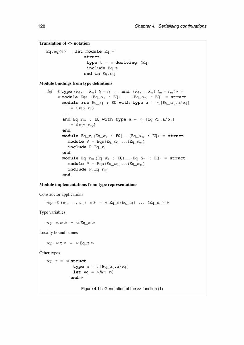
128 Chapter 4. Serialising continuations
Translation of <> notation
Eq.eq<e> = let module Eq =structtype t = e deriving (Eq)include Eq_tend in Eq.eq
Module bindings from type definitions
def <<type (α1,. . .αn) t1 = r1 . . . and (α1,. . .αn) tm = rm >> =<<module Eqs (Eq_α1 : EQ) . . . (Eq_αn : EQ) = struct
module rec Eq_r1 : EQ with type a = r1[Eq_αi.a/αi]= $rep r1$
. . .and Eq_rm : EQ with type a = rm[Eq_αi.a/αi]
= $rep rm$endmodule Eq_r1(Eq_α1 : EQ). . .(Eq_αn : EQ) = struct
module P = Eqs(Eq_α1). . .(Eq_αn)include P.Eq_r1
endmodule Eq_rm(Eq_α1 : EQ). . .(Eq_αn : EQ) = struct
module P = Eqs(Eq_α1). . .(Eq_αn)include P.Eq_rm
end
Module implementations from type representations
Constructor applications
rep <<(a1, . . ., an) c >> = << Eq_c(Eq_a1) . . . (Eq_an)>>
Type variables
rep <<α>> = << Eq_α>>
Locally bound names
rep << t>> = << Eq_t>>
Other types
rep r = <<structtype a = r[Eq_αi.a/αi]let eq = $fun r$
end>>
Figure 4.11: Generation of the eq function (1)
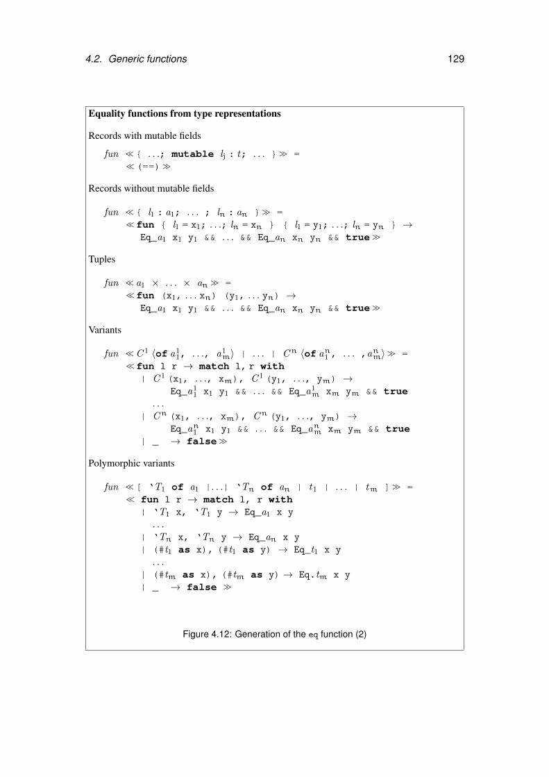
4.2. Generic functions 129
Equality functions from type representations
Records with mutable fields
fun <<{ . . .; mutable lj : t; . . . }>> =<<(==)>>
Records without mutable fields
fun <<{ l1 : a1; . . . ; ln : an }>> =<<fun { l1 = x1; . . .; ln = xn } { l1 = y1; . . .; ln = yn } →
Eq_a1 x1 y1 && . . . && Eq_an xn yn && true>>
Tuples
fun << a1 × . . . × an >> =<<fun (x1, . . . xn) (y1, . . . yn) →
Eq_a1 x1 y1 && . . . && Eq_an xn yn && true>>
Variants
fun <<C 1 〈of a11, . . ., a1
m〉 | . . . | Cn 〈of an1 , . . . ,anm〉>> =<<fun l r → match l, r with
| C 1 (x1, . . ., xm), C 1 (y1, . . ., ym) →Eq_a1
1 x1 y1 && . . . && Eq_a1m xm ym && true
. . .| Cn (x1, . . ., xm), Cn (y1, . . ., ym) →
Eq_an1 x1 y1 && . . . && Eq_anm xm ym && true| _ → false>>
Polymorphic variants
fun <<[ ‘T1 of a1 |. . .| ‘Tn of an | t1 | . . . | tm ]>> =<< fun l r → match l, r with
| ‘T1 x, ‘T1 y → Eq_a1 x y
. . .| ‘Tn x, ‘Tn y → Eq_an x y
| (#t1 as x), (#t1 as y) → Eq_t1 x y
. . .| (#tm as x), (#tm as y)→ Eq.tm x y
| _ → false >>
Figure 4.12: Generation of the eq function (2)
130 Chapter 4. Serialising continuations
module IntSet : sigtype t deriving (Eq)val empty : t
val add : int → t → t
val mem : int → t → bool
end =structtype t = int list
let empty = []let add i l = i :: l
let mem = List.memmodule Eq_t : EQ with type a = t =struct
type a = t
let eq l r = Eq.eq<int list> (sort l) (sort r)end
end
Figure 4.13: Integer sets using integer lists
ing deriving by writing a module definition with a particular name and type instead of adding
the deriving (. . .) annotation to the type. For example, consider the implementation of
integer sets given in Figure 4.13, in which unordered lists of integers are used as the repre-
sentation type. Using deriving we can define equality on IntSet to consider two sets equal if
the results of sorting their representing lists are equal. The builtin equality operator regards
such sets as unequal, exposing the fact that there are various representations for values that the
abstraction considers equivalent:
let onetwo = IntSet.add 1 (IntSet.add 2 (IntSet.empty))let twoone = IntSet.add 2 (IntSet.add 1 (IntSet.empty))
Eq.eq<IntSet.t> onetwo twoone =⇒ trueonetwo = twoone =⇒ false
(Precisely the same problem arises with the set implementation provided in the OCaml standard
library: sets considered equal under the set equality predicate do not always satisfy =.) Using
deriving’s Eq, our abstraction-respecting definition of equality will be used wherever Eq is used
to compare values of IntSet.t; in particular, it will be used where such values occur within a
larger data structure:
Eq.eq<IntSet.t list> [onetwo; twoone] [twoone; onetwo]=⇒ true
4.2. Generic functions 131
4.2.7 Related work
There is a significant body of literature on generic programming. A common approach (Cheney
and Hinze, 2002, Hinze, Löh, and d. S. Oliveira, 2006b, Weirich, 2006) is to reflect types as
values. Generic functions can then be written by case analysis on the structure of these values.
An alternative view (Jansson and Jeuring, 1997, Gibbons, 2006) treats datatypes as fixed points
of regular functors, exposing the recursive structure in a way that allows a variety of traversals
to be expressed generically. A third approach (Lämmel and Peyton Jones, 2003), particularly
suited to generic transformations, uses a type-safe cast operator to locate nodes of particular
types within larger values. Hinze, Jeuring, and Löh (2006a) give a useful comparison of designs
based on these and other approaches.
The preprocessor-based approach to deriving instances of generic functions is used in
the Haskell tools DrIfT (Winstanley, 1997) and Derive (Mitchell and O’Rear, 2006); several
Camlp4 extensions involve the generation of functions from type declarations, including Mar-
tin Jambon’s json-static (Jambon, 2007), Martin Sandin’s Tywith (Sandin, 2004), Daniel de
Rauglaudre’s IoXML (de Rauglaudre, 2002), and Markus Mottl’s bin-prot and sexplib (Mottl,
2007, 2008).
The pickler combinators described in Section 4.1.2.2 are an example of type-indexed val-
ues (Yang, 1998). A type indexed value follows the shape of a type — for example, the
pickler combinator value denoted by list (pair bool bool) corresponds to the ML type
(bool × bool) list — and encodes a function over that type. A similar approach can be
used to encode a wide variety of generic functions in ML. Fernandez, Fisher, Foster, Greenberg,
and Mandelbaum (2008) describe a framework for generic programming based on type-indexed
values in the PADS/ML language, using serialisation to and from XML as the main example.
The main problem in using type-indexed values for generic programming in ML is the
difficulty of combining generic functions. Ideally, we would like to use each type indexed value
to denote not only a pickler at the corresponding type, but also an equality predicate, a printing
function, and any other generic function we might think of. We can, of course, use a distinct
type-indexed value for each generic function, but this rapidly becomes clumsy. The root of
the problem is the lack of higher-kinded polymorphism (i.e. abstraction over non-nullary type
constructors) in ML; given such a facility we could separate the type structure encoded by a
type-indexed value from the particular generic function encoded. Karvonen (2007) describes a
workaround in which generic functions (i.e. type-indexed values) are coded open-recursively
and later combined using the module system. Unfortunately, this only postpones the problem:
before the values can be used there is a “knot-tying” step at which the recursion is closed, at
which point it is no longer possible to incorporate additional generic functions.
132 Chapter 4. Serialising continuations
For the moment, then, the approaches to generic programming that have been used suc-
cessfully in Haskell cannot be ported to OCaml, since they all appear to require advanced
type system features such as generalised algebraic datatypes or higher-kinded polymorphism
that are currently unavailable there. This may change in future if the OCaml team’s plans
for supporting first-class modules come to fruition. First-class modules (Russo, 2000) allow
the encoding of certain types of higher-kinded polymorphism (albeit with a relatively high de-
gree of syntactic overhead), which should make it possible to support fully-combinable generic
functions. At that point it will be time to revisit the design of deriving.
4.3 Generic serialisation
We now return to the subject of serialisation introduced in Section 4.1.
As we indicated earlier, our aim is to construct a serialiser that is suitable as a basis for
implementing the primitive Formlet function pickle_cont. Before we move on to the design
of our serialiser, it may be helpful to note the various “levels” involved in the implementation.
At the outermost level, pickle_cont is a primitive Links function that is used to implement the
Links library for constructing HTML forms. At the next level down, the serialisation functions
on which pickle_cont is built are written in OCaml; they consequently operate on OCaml
values (in the case under consideration, on the first-order representation of Links functions
that is used within the Links prototype). Finally, these serialisation functions are generated
during the compilation of an OCaml program (in our case, during the compilation of the Links
prototype) by the Camlp4 preprocessor. We should perhaps also note that, while implementing
serialisation for Links was the motivation for deriving, there is nothing Links-specific in any
of the generic functions described in this chapter, including the generic serialisers which we
describe in this section.
There are two serialisation schemes provided as standard with deriving: Dump, a simple
value-oriented serialiser, and Pickle, a more realistic serialiser based on Dump, which supports
features such as compression, structure-sharing and serialisation of cyclic values. We restrict
our attention here to the Pickle class.
The essential idea behind Pickle is to build a graph representing a value which is writ-
ten out (using Dump) when complete. Pickle endeavours to maximise sharing, using a single
representation for multiple values, by commencing the serialisation of each value with a com-
parison to values of the same type which have been serialised already. This strategy results
in compact output, but a relatively slower serialiser; however, it is straightforward to obtain
a faster serialisation algorithm which only preserves (rather than introduces) sharing from the
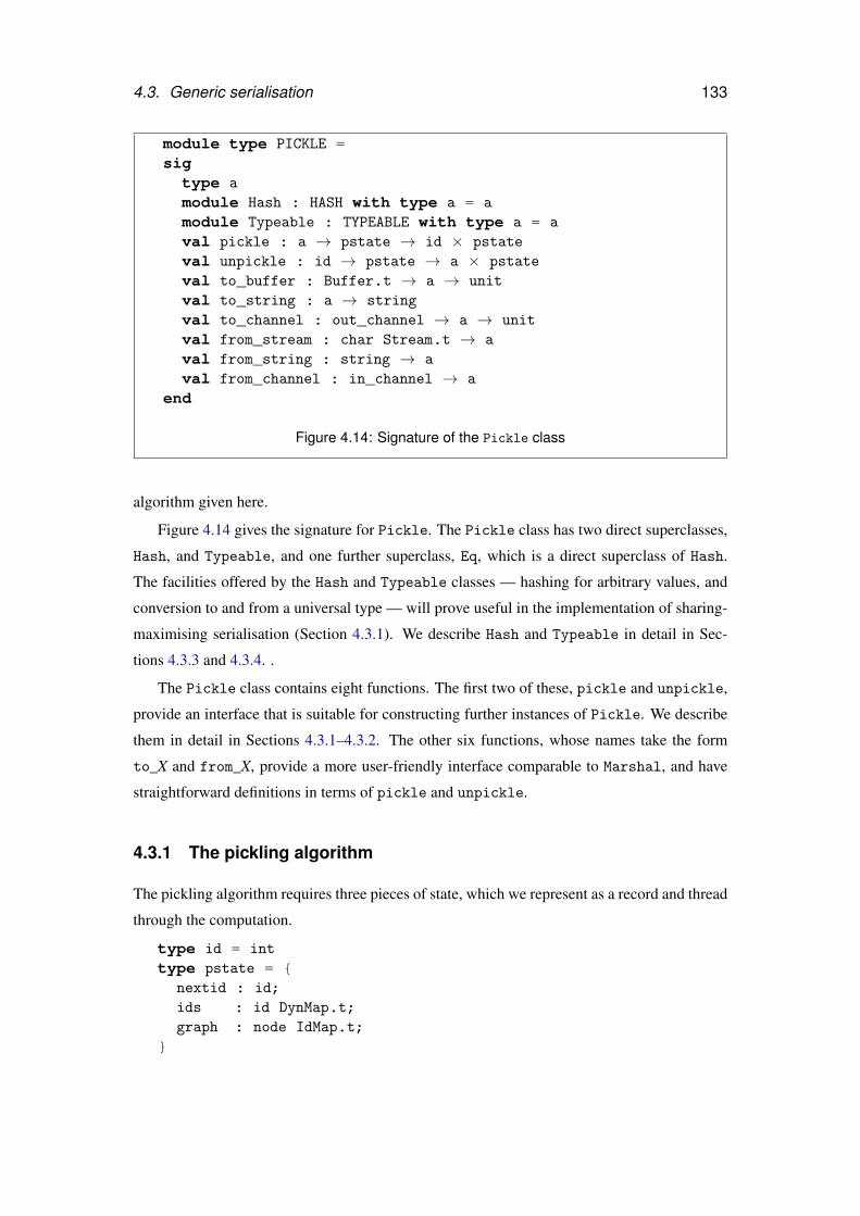
4.3. Generic serialisation 133
module type PICKLE =sigtype a
module Hash : HASH with type a = a
module Typeable : TYPEABLE with type a = a
val pickle : a → pstate → id × pstate
val unpickle : id → pstate → a × pstate
val to_buffer : Buffer.t → a → unit
val to_string : a → string
val to_channel : out_channel → a → unit
val from_stream : char Stream.t → a
val from_string : string → a
val from_channel : in_channel → a
end
Figure 4.14: Signature of the Pickle class
algorithm given here.
Figure 4.14 gives the signature for Pickle. The Pickle class has two direct superclasses,
Hash, and Typeable, and one further superclass, Eq, which is a direct superclass of Hash.
The facilities offered by the Hash and Typeable classes — hashing for arbitrary values, and
conversion to and from a universal type — will prove useful in the implementation of sharing-
maximising serialisation (Section 4.3.1). We describe Hash and Typeable in detail in Sec-
tions 4.3.3 and 4.3.4. .
The Pickle class contains eight functions. The first two of these, pickle and unpickle,
provide an interface that is suitable for constructing further instances of Pickle. We describe
them in detail in Sections 4.3.1–4.3.2. The other six functions, whose names take the form
to_X and from_X, provide a more user-friendly interface comparable to Marshal, and have
straightforward definitions in terms of pickle and unpickle.
4.3.1 The pickling algorithm
The pickling algorithm requires three pieces of state, which we represent as a record and thread
through the computation.
type id = int
type pstate = {nextid : id;ids : id DynMap.t;graph : node IdMap.t;
}
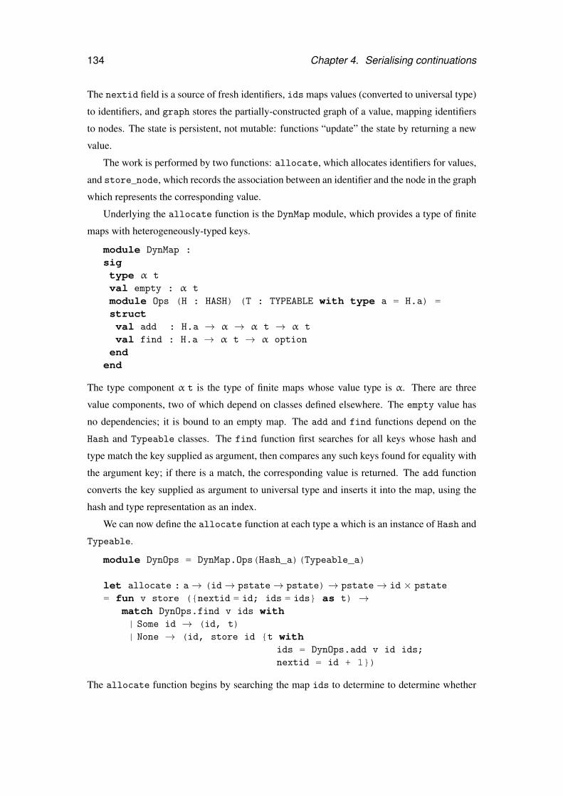
134 Chapter 4. Serialising continuations
The nextid field is a source of fresh identifiers, ids maps values (converted to universal type)
to identifiers, and graph stores the partially-constructed graph of a value, mapping identifiers
to nodes. The state is persistent, not mutable: functions “update” the state by returning a new
value.
The work is performed by two functions: allocate, which allocates identifiers for values,
and store_node, which records the association between an identifier and the node in the graph
which represents the corresponding value.
Underlying the allocate function is the DynMap module, which provides a type of finite
maps with heterogeneously-typed keys.
module DynMap :sigtype α t
val empty : α t
module Ops (H : HASH) (T : TYPEABLE with type a = H.a) =structval add : H.a → α → α t → α t
val find : H.a → α t → α option
endend
The type component α t is the type of finite maps whose value type is α. There are three
value components, two of which depend on classes defined elsewhere. The empty value has
no dependencies; it is bound to an empty map. The add and find functions depend on the
Hash and Typeable classes. The find function first searches for all keys whose hash and
type match the key supplied as argument, then compares any such keys found for equality with
the argument key; if there is a match, the corresponding value is returned. The add function
converts the key supplied as argument to universal type and inserts it into the map, using the
hash and type representation as an index.
We can now define the allocate function at each type a which is an instance of Hash and
Typeable.
module DynOps = DynMap.Ops(Hash_a)(Typeable_a)
let allocate : a→ (id→ pstate→ pstate)→ pstate→ id × pstate
= fun v store ({nextid = id; ids = ids} as t) →match DynOps.find v ids with| Some id → (id, t)| None → (id, store id {t with
ids = DynOps.add v id ids;nextid = id + 1})
The allocate function begins by searching the map ids to determine to determine whether
4.3. Generic serialisation 135
the value has been previously serialised. If it finds a match it returns the identifier already
allocated; if there is no match then a fresh identifier is allocated, the association between iden-
tifier and value is recorded using add and the function store is called to serialise the value.
This strategy of allocating identifiers before serialising subvalues is sufficient for serialisation
of cyclic values: the next time a reference to this node is encountered there will be an identifier
in the map, so serialisation will not loop.
The store_node function simply records the association between an identifier and a node.
let store_node : node → id → pstate → pstate
= fun node id state →{state with graph = IdMap.add id node state.graph}
Nodes of the graph are represented as values of the node type. A node is either a sequence
of bytes (representing a primitive value such as an integer or a string), or a value of algebraic
type, which is represented as an optional index for the constructor and a sequence of identifiers
for the subvalues.
type node = Bytes of string
| Appl of int option × id list
deriving (Dump)
Once the graph has been fully constructed we discard the other components of the state
record. In order to reduce the size of the serialised data we first change the representation of
the graph. As we have seen, during construction the graph takes the form of a finite map from
identifiers to node values. Serialising this directly takes up an unnecessarily large amount of
space, since we must serialise an identifier and a constructor (representing either Bytes or
Appl) alongside every node. We eliminate the need to serialise constructors by changing the
representation to use three maps, one for each of the three constructor configurations (Bytes,
Appl with a constructor index, and Appl without a constructor index). For example, pickling
might construct the following graph:
{1 ⇒ Appl (Some 2, [4;3]),2 ⇒ Appl (None, [1;4]),3 ⇒ Bytes "p",4 ⇒ Bytes "k"}
This is replaced with three maps, eliminating the need to store constructors:
{3 ⇒ "p",4 ⇒ "k"}{1 ⇒ (2, [4;3])}{2 ⇒ [1;4]}
Listing the pairs of keys and values sequentially gives the following:
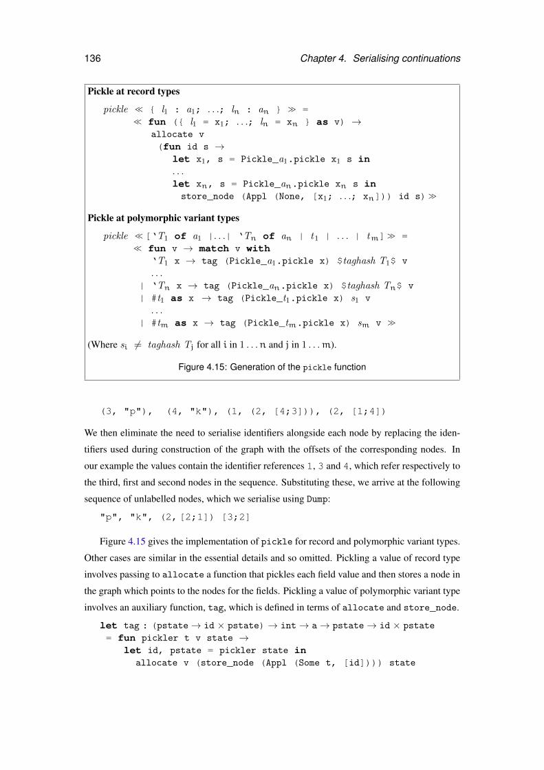
136 Chapter 4. Serialising continuations
Pickle at record types
pickle << { l1 : a1; . . .; ln : an } >> =<< fun ({ l1 = x1; . . .; ln = xn } as v) →
allocate v
(fun id s →let x1, s = Pickle_a1.pickle x1 s in. . .let xn, s = Pickle_an.pickle xn s instore_node (Appl (None, [x1; . . .; xn])) id s)>>
Pickle at polymorphic variant types
pickle <<[‘T1 of a1 |. . .| ‘Tn of an | t1 | . . . | tm]>> =<< fun v → match v with
‘T1 x → tag (Pickle_a1.pickle x) $taghash T1$ v
. . .| ‘Tn x → tag (Pickle_an.pickle x) $taghash Tn$ v
| #t1 as x → tag (Pickle_t1.pickle x) s1 v
. . .| #tm as x → tag (Pickle_tm.pickle x) sm v >>
(Where si 6= taghash Tj for all i in 1 . . .n and j in 1 . . .m).
Figure 4.15: Generation of the pickle function
(3, "p"), (4, "k"), (1, (2, [4;3])), (2, [1;4])
We then eliminate the need to serialise identifiers alongside each node by replacing the iden-
tifiers used during construction of the graph with the offsets of the corresponding nodes. In
our example the values contain the identifier references 1, 3 and 4, which refer respectively to
the third, first and second nodes in the sequence. Substituting these, we arrive at the following
sequence of unlabelled nodes, which we serialise using Dump:
"p", "k", (2,[2;1]) [3;2]
Figure 4.15 gives the implementation of pickle for record and polymorphic variant types.
Other cases are similar in the essential details and so omitted. Pickling a value of record type
involves passing to allocate a function that pickles each field value and then stores a node in
the graph which points to the nodes for the fields. Pickling a value of polymorphic variant type
involves an auxiliary function, tag, which is defined in terms of allocate and store_node.
let tag : (pstate→ id × pstate)→ int→ a→ pstate→ id × pstate
= fun pickler t v state →let id, pstate = pickler state in
allocate v (store_node (Appl (Some t, [id]))) state
4.3. Generic serialisation 137
The tag function takes as argument an function, pickler, which stores a value v; it returns
a function which stores a tagged value ‘T v. The second parameter, t, denotes the tag T; the
third parameter is the complete value to be stored, ‘T v.
A polymorphic variant type can be declared in any of a number of compatible ways. In
particular, the order of tags does not affect the denotation of the type: [‘A | ‘B] is compat-
ible with [‘B | ‘A], and both may be used to denote the same type within a single program
(Section 4.3.3). In assigning numbers to tags, therefore, we cannot simply use the order in
which the tags appear in the declaration. Instead we use a hash of each tag name, ensuring that
the mapping from tags to integers is globally consistent. The hash function we use is the same
function used by the OCaml compiler to represent polymorphic variant tags (Garrigue, 1998).
The type checker rejects types containing tags, such as ‘squigglier and ‘premiums, whose
hash numbers collide. Using the same hash function as OCaml therefore ensures that we will
not be troubled by collisions. In the case where a polymorphic variant type t extends some
other type s we assign a tag number to s that does not collide with the hashes of the other tags
of t.
4.3.2 The unpickling algorithm
Detecting cycles is straightforward; reconstructing cycles is trickier. Values in OCaml are
constructed from subvalues: the subvalues must exist first, but this breaks down if the value
is among its own subvalues (either directly or as a more distant descendent). As we saw in
Section 4.1.2.2, Elsman solves this problem by requiring the user to supply an initial value to
start the recursion going. Our solution is to use low-level primitives to allocate an uninitialised
value whose address can be used in constructing subvalues. In generated code the risk of a
mistake in such memory manipulation is low, whilst the advantages — increased abstraction
and ease of use — are great.
Like the pickling algorithm, the unpickling algorithm threads a piece of state throughout
the computation. The state we need is a finite map whose keys are identifiers and whose values
are either node representations of values or fully deserialised values, represented using the
universal type, dynamic.
type ustate = ((node, dynamic) either) IdMap.t
At the start of unpickling, every value in the map is a node. The unpickling process replaces
each of these with fully reconstructed values.
The unpickling algorithm is based on two combinators, variant and record, which per-
form unpickling for particular types and update the state.
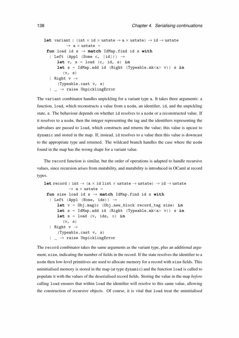
138 Chapter 4. Serialising continuations
let variant : (int × id × ustate→ a × ustate)→ id→ ustate
→ a × ustate =fun load id s → match IdMap.find id s with| Left (Appl (Some c, [id])) →
let v, s = load (c, id, s) inlet s = IdMap.add id (Right (Typeable.mk<a> v)) s in(v, s)
| Right v →(Typeable.cast v, s)
| _ → raise UnpicklingError
The variant combinator handles unpickling for a variant type a. It takes three arguments: a
function, load, which reconstructs a value from a node, an identifier, id, and the unpickling
state, s. The behaviour depends on whether id resolves to a node or a reconstructed value. If
it resolves to a node, then the integer representing the tag and the identifiers representing the
subvalues are passed to load, which constructs and returns the value; this value is upcast to
dynamic and stored in the map. If, instead, id resolves to a value then this value is downcast
to the appropriate type and returned. The wildcard branch handles the case where the node
found in the map has the wrong shape for a variant value.
The record function is similar, but the order of operations is adapted to handle recursive
values, since recursion arises from mutability, and mutability is introduced in OCaml at record
types.
let record : int→ (a × id list × ustate→ ustate)→ id→ ustate
→ a × ustate =fun size load id s → match IdMap.find id s with| Left (Appl (None, ids)) →
let v = Obj.magic (Obj.new_block record_tag size) inlet s = IdMap.add id (Right (Typeable.mk<a> v)) s inlet s = load (v, ids, s) in
(v, s)| Right v →
(Typeable.cast v, s)| _ → raise UnpicklingError
The record combinator takes the same arguments as the variant type, plus an additional argu-
ment, size, indicating the number of fields in the record. If the state resolves the identifier to a
node then low-level primitives are used to allocate memory for a record with size fields. This
uninitialised memory is stored in the map (at type dynamic) and the function load is called to
populate it with the values of the deserialised record fields. Storing the value in the map before
calling load ensures that within load the identifier will resolve to this same value, allowing
the construction of recursive objects. Of course, it is vital that load treat the uninitialised
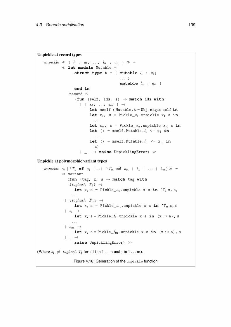
4.3. Generic serialisation 139
Unpickle at record types
unpickle << { l1 : a1; . . .; ln : an } >> =<< let module Mutable =
struct type t = { mutable l1 : a1;. . . ;mutable ln : an }
end inrecord n(fun (self, ids, s) → match ids with| [ x1; . . .; xn ] →
let mself : Mutable.t = Obj.magic self inlet x1, s = Pickle_a1.unpickle x1 s in
. . .let xn, s = Pickle_an.unpickle xn s inlet () = mself.Mutable.l1 <- x1 in
. . .let () = mself.Mutable.ln <- xn in
s)| _ → raise UnpicklingError) >>
Unpickle at polymorphic variant types
unpickle <<[‘T1 of a1 |. . .| ‘Tn of an | t1 | . . . | tm]>> =<< variant
(fun (tag, x, s → match tag with$taghash T1$ →let x, s = Pickle_a1.unpickle x s in ‘T1 x, s,
. . .| $taghash Tn$ →
let x, s = Pickle_an.unpickle x s in ‘Tn x, s| s1 →
let x, s = Pickle_t1.unpickle x s in (x :> a), s. . .
| sm →let x, s = Pickle_tm.unpickle x s in (x :> a), s
| _ →raise UnpicklingError) >>
(Where si 6= taghash Tj for all i in 1 . . .n and j in 1 . . .m).
Figure 4.16: Generation of the unpickle function
140 Chapter 4. Serialising continuations
value as “write-only”; this is guaranteed by the unpickling algorithm, which does not inspect
deserialised values.
Figure 4.16 gives the implementation of unpickle for record and polymorphic variant
types. The generated function for a record type r includes the declaration of a type structurally
similar to r, but with every field declared mutable. The function passed to record receives an
uninitialised value of sufficient size, together with identifiers for the fields, and the state. The
function casts the uninitialised value, self, to the mutable type, which makes it possible to
first reconstruct subvalues which may contain references to self, then assign the subvalues to
the fields of self.
The unpickle function for polymorphic variants is straightforward: first the argument of
each tag is reconstructed, then the tag is applied to the reconstructed value. The tag numbers
s1 . . . sm used for the types t1 . . . tm must, of course, match those generated for use in the
pickle function (Figure 4.15).
4.3.2.1 Immutable cycles
The approach we describe here is sufficient to handle all cycles based on mutability; there is no
attempt to handle the immutable cycles which arise from OCaml’s value recursion extension.
This extension permits non-function values on the right-hand-side of let rec bindings, so
long as they meet certain syntactic restrictions which prevent reading partially constructed
values. For example, the declaration
let rec x = 1 :: 2 :: x
binds x to a cyclic list of integers whose values alternate between 1 and 2. Values of this form
cause unpickling to loop.
However, as a side effect of the implementation, unpickling will successfully reconstruct
immutable cyclic objects where the cycles pass through records. For example, given the type
declaration
type α cons = { car : α ; cdr : α seq }and α seq = Cons of α cons
deriving (Eq, Hash, Typeable, Pickle)
the following declaration for y creates a cyclic value that can be pickled and unpickled without
problems.
let rec y = Cons { car = 1; cdr = Cons { car = 2; cdr = y}}
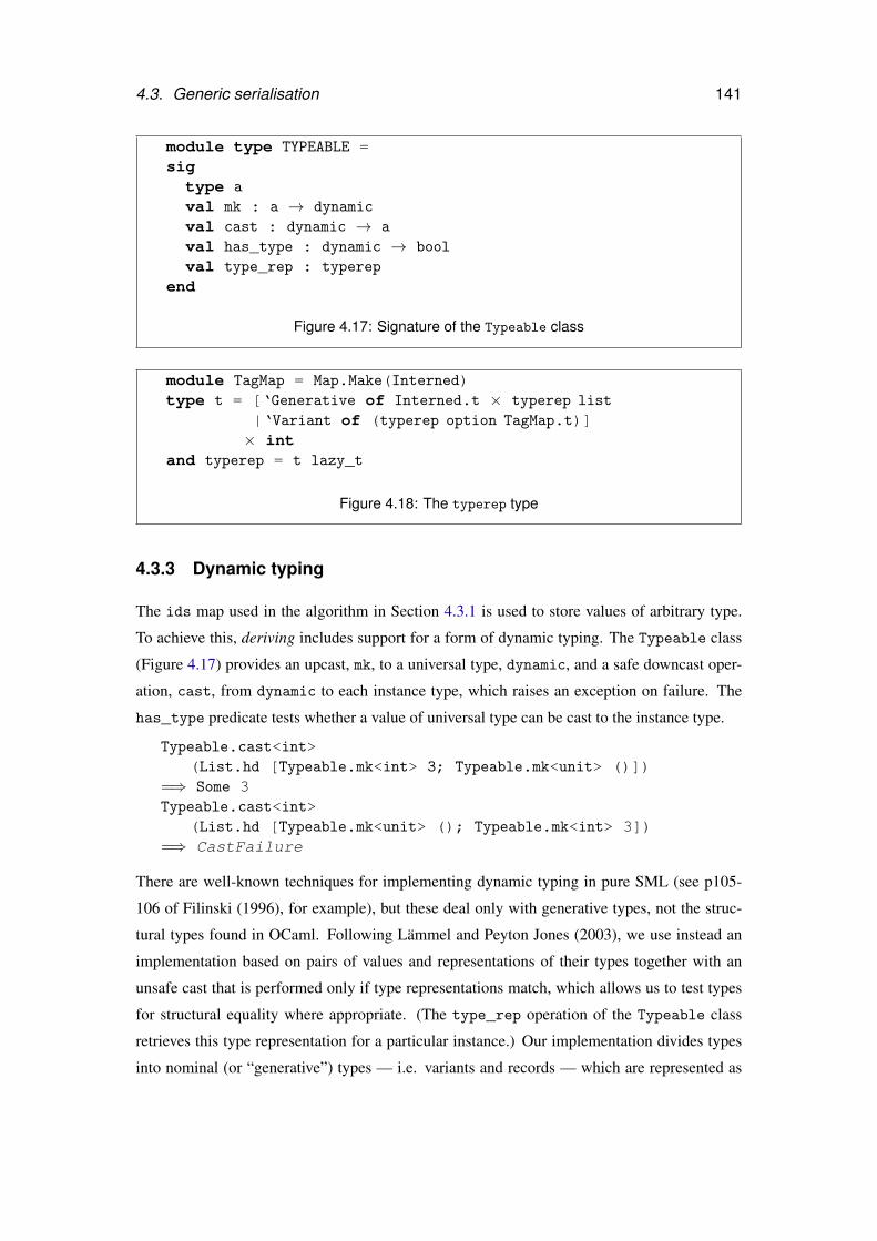
4.3. Generic serialisation 141
module type TYPEABLE =sig
type a
val mk : a → dynamic
val cast : dynamic → a
val has_type : dynamic → bool
val type_rep : typerep
end
Figure 4.17: Signature of the Typeable class
module TagMap = Map.Make(Interned)type t = [‘Generative of Interned.t × typerep list
|‘Variant of (typerep option TagMap.t)]× int
and typerep = t lazy_t
Figure 4.18: The typerep type
4.3.3 Dynamic typing
The ids map used in the algorithm in Section 4.3.1 is used to store values of arbitrary type.
To achieve this, deriving includes support for a form of dynamic typing. The Typeable class
(Figure 4.17) provides an upcast, mk, to a universal type, dynamic, and a safe downcast oper-
ation, cast, from dynamic to each instance type, which raises an exception on failure. The
has_type predicate tests whether a value of universal type can be cast to the instance type.
Typeable.cast<int>(List.hd [Typeable.mk<int> 3; Typeable.mk<unit> ()])
=⇒ Some 3Typeable.cast<int>
(List.hd [Typeable.mk<unit> (); Typeable.mk<int> 3])=⇒ CastFailure
There are well-known techniques for implementing dynamic typing in pure SML (see p105-
106 of Filinski (1996), for example), but these deal only with generative types, not the struc-
tural types found in OCaml. Following Lämmel and Peyton Jones (2003), we use instead an
implementation based on pairs of values and representations of their types together with an
unsafe cast that is performed only if type representations match, which allows us to test types
for structural equality where appropriate. (The type_rep operation of the Typeable class
retrieves this type representation for a particular instance.) Our implementation divides types
into nominal (or “generative”) types — i.e. variants and records — which are represented as
142 Chapter 4. Serialising continuations
a string for the type constructor and a sequence of argument types, and structural types —
i.e. polymorphic variants— which are represented as lazy infinite trees. Tuples are treated as
nominal, using the arity as the type constructor. The concrete definition of typerep is given
in Figure 4.18. We use interned strings, with constant-time equality testing, to represent gener-
ative types and polymorphic variant tags. A final point to note is that type representations are
lazy. Laziness allows us to construct recursive type representations for recursive types; without
laziness our attempts to construct such representations are rejected as unsafe, since they do
not meet the syntactic restrictions mentioned in Section 4.3.2.1. Syme (2006) gives a general
account of using laziness to introduce recursion in this way.
The definition of equality on type representations corresponds closely to the OCaml defini-
tion of equality on types. Nominal types are considered equal if they have the same constructors
and equal arguments. Polymorphic variant types are considered equal if they have the same set
of labels and if the arguments to corresponding labels are equal. Recursive polymorphic variant
types have cyclic representations; termination of the equality test is assured by associating an
identifier with each node — the int component of the type representation — which is used to
record which nodes have been visited, i.e. to detect cycles. Since polymorphic variant types
are always regular all recursion eventually passes through an already visited node.
Polymorphic variant types which are considered equivalent in the OCaml type system are
treated as equivalent by deriving regardless of how they are declared, so the following cast will
succeed:
type α seq = [‘Nil | ‘Cons of α × α seq]deriving (Typeable)
type nil = [‘Nil]deriving (Typeable)
type intlist = [ nil | ‘Cons of int × α ] as α
deriving (Typeable)
Typeable.cast<intlist>(Typeable.mk<int seq>
(‘Cons (1, ‘Cons (2, ‘Cons (3, ‘Nil)))))=⇒ Some (‘Cons (1, ‘Cons (2, ‘Cons (3, ‘Nil))))
Similarly, the type representation used by Typeable does not respect module abstraction bound-
aries, so the following cast also succeeds:
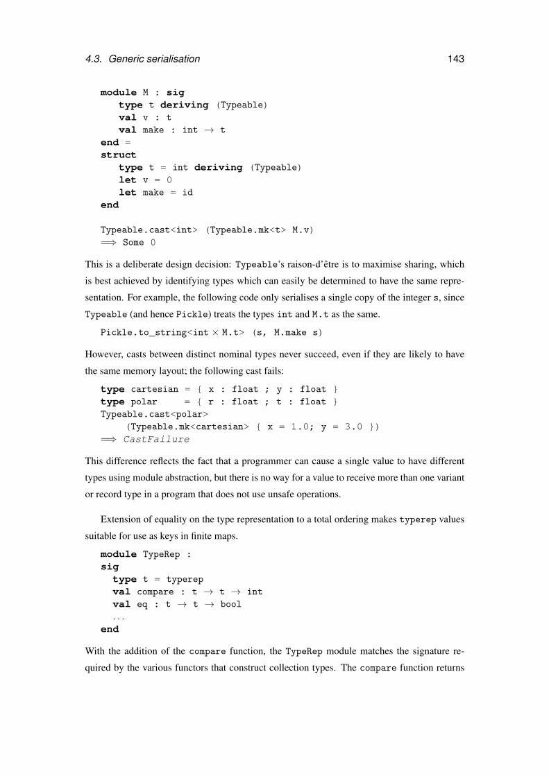
4.3. Generic serialisation 143
module M : sigtype t deriving (Typeable)val v : t
val make : int → t
end =struct
type t = int deriving (Typeable)let v = 0let make = id
end
Typeable.cast<int> (Typeable.mk<t> M.v)=⇒ Some 0
This is a deliberate design decision: Typeable’s raison-d’être is to maximise sharing, which
is best achieved by identifying types which can easily be determined to have the same repre-
sentation. For example, the following code only serialises a single copy of the integer s, since
Typeable (and hence Pickle) treats the types int and M.t as the same.
Pickle.to_string<int × M.t> (s, M.make s)
However, casts between distinct nominal types never succeed, even if they are likely to have
the same memory layout; the following cast fails:
type cartesian = { x : float ; y : float }type polar = { r : float ; t : float }Typeable.cast<polar>
(Typeable.mk<cartesian> { x = 1.0; y = 3.0 })=⇒ CastFailure
This difference reflects the fact that a programmer can cause a single value to have different
types using module abstraction, but there is no way for a value to receive more than one variant
or record type in a program that does not use unsafe operations.
Extension of equality on the type representation to a total ordering makes typerep values
suitable for use as keys in finite maps.
module TypeRep :sigtype t = typerep
val compare : t → t → int
val eq : t → t → bool
. . .end
With the addition of the compare function, the TypeRep module matches the signature re-
quired by the various functors that construct collection types. The compare function returns
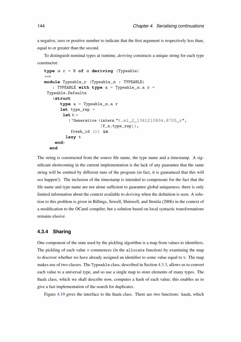
144 Chapter 4. Serialising continuations
a negative, zero or positive number to indicate that the first argument is respectively less than,
equal to or greater than the second.
To distinguish nominal types at runtime, deriving constructs a unique string for each type
constructor:
type α r = R of α deriving (Typeable)=⇒module Typeable_r (Typeable_α : TYPEABLE)
: TYPEABLE with type a = Typeable_α.a r =Typeable.Defaults(struct
type a = Typeable_α.a r
let type_rep =let t =
(‘Generative (intern "t.ml_2_1381210804.8705_r",[V_a.type_rep]),
fresh_id ()) inlazy t
end)end
The string is constructed from the source file name, the type name and a timestamp. A sig-
nificant shortcoming in the current implementation is the lack of any guarantee that the same
string will be emitted by different runs of the program (in fact, it is guaranteed that this will
not happen!). The inclusion of the timestamp is intended to compensate for the fact that the
file name and type name are not alone sufficient to guarantee global uniqueness; there is only
limited information about the context available to deriving when the definition is seen. A solu-
tion to this problem is given in Billings, Sewell, Shinwell, and Strniša (2006) in the context of
a modification to the OCaml compiler, but a solution based on local syntactic transformations
remains elusive.
4.3.4 Sharing
One component of the state used by the pickling algorithm is a map from values to identifiers.
The pickling of each value v commences (in the allocate function) by examining the map
to discover whether we have already assigned an identifier to some value equal to v. The map
makes use of two classes. The Typeable class, described in Section 4.3.3, allows us to convert
each value to a universal type, and so use a single map to store elements of many types. The
Hash class, which we shall describe now, computes a hash of each value; this enables us to
give a fast implementation of the search for duplicates.
Figure 4.19 gives the interface to the Hash class. There are two functions: hash, which
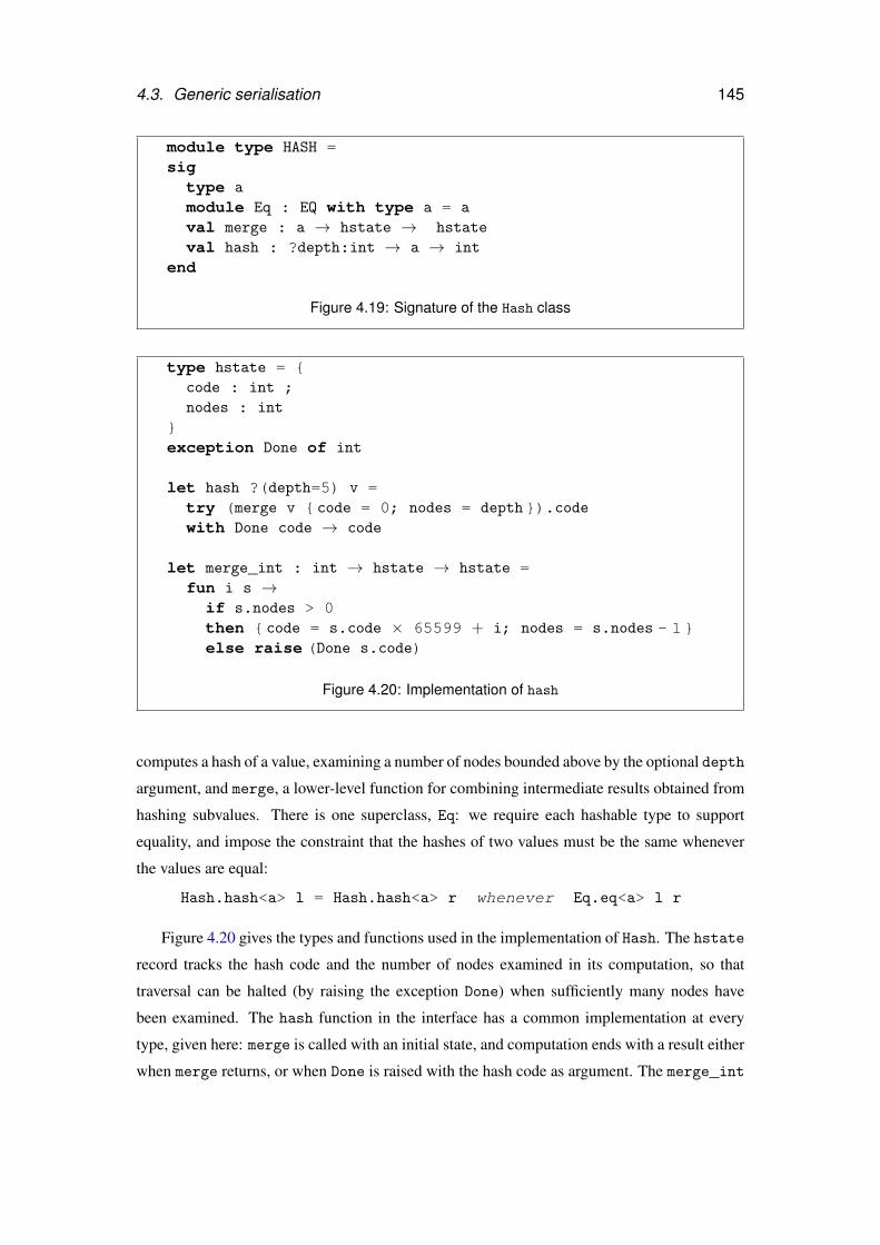
4.3. Generic serialisation 145
module type HASH =sigtype a
module Eq : EQ with type a = a
val merge : a → hstate → hstate
val hash : ?depth:int → a → int
end
Figure 4.19: Signature of the Hash class
type hstate = {code : int ;nodes : int
}exception Done of int
let hash ?(depth=5) v =try (merge v { code = 0; nodes = depth}).codewith Done code → code
let merge_int : int → hstate → hstate =fun i s →
if s.nodes > 0then { code = s.code × 65599 + i; nodes = s.nodes - 1}else raise (Done s.code)
Figure 4.20: Implementation of hash
computes a hash of a value, examining a number of nodes bounded above by the optional depth
argument, and merge, a lower-level function for combining intermediate results obtained from
hashing subvalues. There is one superclass, Eq: we require each hashable type to support
equality, and impose the constraint that the hashes of two values must be the same whenever
the values are equal:
Hash.hash<a> l = Hash.hash<a> r whenever Eq.eq<a> l r
Figure 4.20 gives the types and functions used in the implementation of Hash. The hstate
record tracks the hash code and the number of nodes examined in its computation, so that
traversal can be halted (by raising the exception Done) when sufficiently many nodes have
been examined. The hash function in the interface has a common implementation at every
type, given here: merge is called with an initial state, and computation ends with a result either
when merge returns, or when Done is raised with the hash code as argument. The merge_int
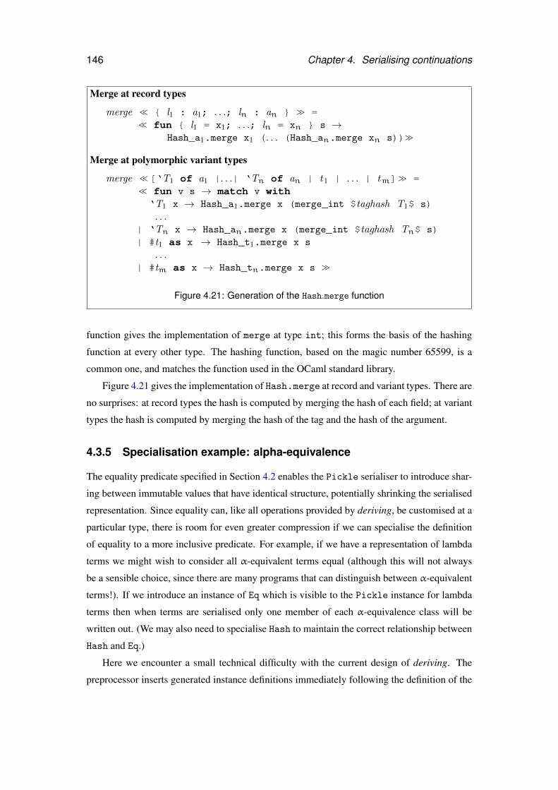
146 Chapter 4. Serialising continuations
Merge at record types
merge << { l1 : a1; . . .; ln : an } >> =<< fun { l1 = x1; . . .; ln = xn } s →
Hash_a1.merge x1 (. . . (Hash_an.merge xn s))>>
Merge at polymorphic variant types
merge <<[‘T1 of a1 |. . .| ‘Tn of an | t1 | . . . | tm]>> =<< fun v s → match v with‘T1 x → Hash_a1.merge x (merge_int $taghash T1$ s)
. . .| ‘Tn x → Hash_an.merge x (merge_int $taghash Tn$ s)| #t1 as x → Hash_t1.merge x s
. . .| #tm as x → Hash_tn.merge x s >>
Figure 4.21: Generation of the Hash.merge function
function gives the implementation of merge at type int; this forms the basis of the hashing
function at every other type. The hashing function, based on the magic number 65599, is a
common one, and matches the function used in the OCaml standard library.
Figure 4.21 gives the implementation of Hash.merge at record and variant types. There are
no surprises: at record types the hash is computed by merging the hash of each field; at variant
types the hash is computed by merging the hash of the tag and the hash of the argument.
4.3.5 Specialisation example: alpha-equivalence
The equality predicate specified in Section 4.2 enables the Pickle serialiser to introduce shar-
ing between immutable values that have identical structure, potentially shrinking the serialised
representation. Since equality can, like all operations provided by deriving, be customised at a
particular type, there is room for even greater compression if we can specialise the definition
of equality to a more inclusive predicate. For example, if we have a representation of lambda
terms we might wish to consider all α-equivalent terms equal (although this will not always
be a sensible choice, since there are many programs that can distinguish between α-equivalent
terms!). If we introduce an instance of Eq which is visible to the Pickle instance for lambda
terms then when terms are serialised only one member of each α-equivalence class will be
written out. (We may also need to specialise Hash to maintain the correct relationship between
Hash and Eq.)
Here we encounter a small technical difficulty with the current design of deriving. The
preprocessor inserts generated instance definitions immediately following the definition of the
4.3. Generic serialisation 147
associated type. Further, since Eq is a superclass of Pickle, the Eq instance for a type must be
visible within its Pickle instance. Our definition of Eq must follow the type definition for the
constructors to be visible, but the preprocessor will insert the Pickle definition between the
definition of the type and our definition of Eq (which the preprocessor ignores). We can dodge
the difficulty using a recursive module, which allows us to bring a definition of Eq into scope
within the preceding Pickle definition, but this is a rather distasteful necessity. We plan to
address the difficulty in future versions of deriving.
Figure 4.22 defines a datatype, exp, for representing lambda terms, together with spe-
cialised instances for Eq and Hash that are visible to the generated instance for Pickle. The
Eq instance uses α-equivalence, rather than structural equality; the Hash instance correspond-
ingly ignores variable names, computing a hash based on constructors only. Parts (a) and (b)
of Figure 4.23 show the sharing introduced by Pickle for a particular lambda term (a call-by-
value fixpoint combinator) represented as a value of exp.
There is one further opportunity to increase the potential for sharing. OCaml strings are
mutable, so the default definition of equality compares their physical addresses rather than their
contents. A value-oriented instance of Eq for strings (taking OCaml’s = for eq) leads to further
sharing under Pickle, as seen in Figure 4.23 (c). In order to change the predicate used to
compare strings we can define a type alias for string, istring, and a module Eq_istring,
and replace the references to string in the definition of exp with references to istring.
type istring = string
module Eq_istring = structtype a = istring
let eq = (=)end. . .type exp = Var of istring
| App of exp× exp
| Lam of istring× exp
deriving (Eq)
This definition allows Eq.eq<exp> to use structural equality for string comparisons, but has
no effect on the rest of the program. Our notation for overloaded operations is generally more
cumbersome than in a language such as Haskell where there is no need to specify the type at
each call. In this case the burden becomes an advantage: deriving selects instances according to
the declared name of a type, so we can use different instances for a given type at various points
in the program by introducing a type alias for each instance. (A similar point is made in Dreyer
et al. (2007), which couples Haskell-style overloading with an operation for explicitly making
a particular instance “canonical” in a certain scope.)
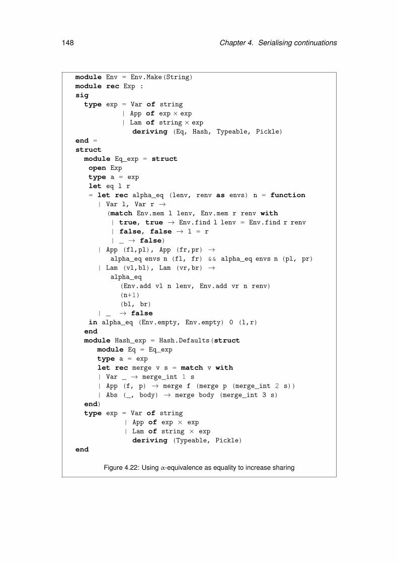
148 Chapter 4. Serialising continuations
module Env = Env.Make(String)module rec Exp :sigtype exp = Var of string
| App of exp × exp
| Lam of string × exp
deriving (Eq, Hash, Typeable, Pickle)end =structmodule Eq_exp = structopen Exp
type a = exp
let eq l r
= let rec alpha_eq (lenv, renv as envs) n = function| Var l, Var r →
(match Env.mem l lenv, Env.mem r renv with| true, true → Env.find l lenv = Env.find r renv
| false, false → l = r
| _ → false)| App (fl,pl), App (fr,pr) →
alpha_eq envs n (fl, fr) && alpha_eq envs n (pl, pr)| Lam (vl,bl), Lam (vr,br) →
alpha_eq(Env.add vl n lenv, Env.add vr n renv)(n+1)(bl, br)
| _ → falsein alpha_eq (Env.empty, Env.empty) 0 (l,r)
endmodule Hash_exp = Hash.Defaults(struct
module Eq = Eq_exptype a = exp
let rec merge v s = match v with| Var _ → merge_int 1 s
| App (f, p) → merge f (merge p (merge_int 2 s))| Abs (_, body) → merge body (merge_int 3 s)
end)type exp = Var of string
| App of exp × exp
| Lam of string × exp
deriving (Typeable, Pickle)end
Figure 4.22: Using α-equivalence as equality to increase sharing
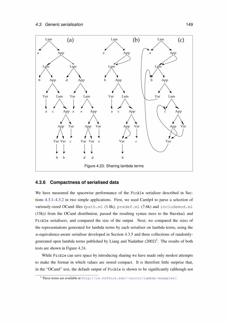
4.3. Generic serialisation 149
d dbb
AppVar VarApp
AppApp ea c a
LamLamVar Var
LamLam
Var VarVarVar ec
AppAppb d
Lam
Appa
(a)
Lam
Var c
Appb
Lam
Appa
VarApp
Appa c
LamVar
b
(b)
Lam
Var
Appb
Lam
Appa
VarApp
Appc
LamVar
(c)
mar
Figure 4.23: Sharing lambda terms
4.3.6 Compactness of serialised data
We have measured the spacewise performance of the Pickle serialiser described in Sec-
tions 4.3.1–4.3.2 in two simple applications. First, we used Camlp4 to parse a selection of
variously-sized OCaml files (path.ml (1.8k), predef.ml (7.6k) and includemod.ml
(15k)) from the OCaml distribution, passed the resulting syntax trees to the Marshal and
Pickle serialisers, and compared the size of the output. Next, we compared the sizes of
the representations generated for lambda terms by each serialiser on lambda terms, using the
α-equivalence-aware serialiser developed in Section 4.3.5 and three collections of randomly-
generated open lambda terms published by Liang and Nadathur (2002)3. The results of both
tests are shown in Figure 4.24.
While Pickle can save space by introducing sharing we have made only modest attempts
to make the format in which values are stored compact. It is therefore little surprise that,
in the “OCaml” test, the default output of Pickle is shown to be significantly (although not
3 These terms are available at http://cs.hofstra.edu/~cscccl/lambda-examples/.
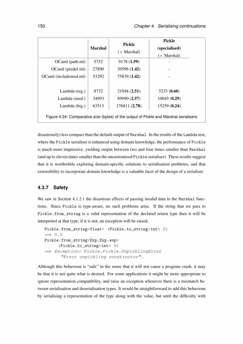
150 Chapter 4. Serialising continuations
MarshalPickle
(×Marshal)
Pickle
(specialised)
(×Marshal)OCaml (path.ml) 5752 9178 (1.59) -
OCaml (predef.ml) 27890 39596 (1.42) -
OCaml (includemod.ml) 53292 75839 (1.42) -
Lambda (reg.) 8732 21948 (2.51) 5233 (0.60)
Lambda (med.) 34993 89990 (2.57) 10045 (0.29)
Lambda (big.) 63513 176811 (2.78) 15259 (0.24)
Figure 4.24: Comparative size (bytes) of the output of Pickle and Marshal serialisers
disastrously) less compact than the default output of Marshal. In the results of the Lambda test,
where the Pickle serialiser is enhanced using domain knowledge, the performance of Pickle
is much more impressive, yielding output between two and four times smaller than Marshal
(and up to eleven times smaller than the uncustomised Pickle serialiser). These results suggest
that it is worthwhile exploring domain-specific solutions to serialisation problems, and that
extensibility to incorporate domain knowledge is a valuable facet of the design of a serialiser.
4.3.7 Safety
We saw in Section 4.1.2.1 the disastrous effects of passing invalid data to the Marshal func-
tions. Since Pickle is type-aware, no such problems arise. If the string that we pass to
Pickle.from_string is a valid representation of the declared return type then it will be
interpreted at that type; if it is not, an exception will be raised.
Pickle.from_string<float> (Pickle.to_string<int> 0)=⇒ 0.0Pickle.from_string<Exp.Exp.exp>
(Pickle.to_string<int> 0)=⇒ Exception: Pickle.Pickle.UnpicklingError
"Error unpickling constructor".
Although this behaviour is “safe” in the sense that it will not cause a program crash, it may
be that it is not quite what is desired. For some applications it might be more appropriate to
ignore representation compatibility, and raise an exception whenever there is a mismatch be-
tween serialisation and deserialisation types. It would be straightforward to add this behaviour
by serialising a representation of the type along with the value, but until the difficulty with

4.4. Conclusions and future work 151
mapping type constructors to unique names described in Section 4.3.3 is resolved it would
only be possible to check equality of serialised types within the same compiled instance of the
program which produced them.
4.3.8 Related work
The serialisation problem has received considerable attention in the ML community. The Hash-
Caml (Billings et al., 2006) project extends the OCaml bytecode compiler with type-passing to
make the standard Marshal operation type-safe. Cohen and Herrmann (Cohen and Herrmann,
2005) discuss the implementation of a staged serialiser in MetaOCaml which bears some sim-
ilarity to our preprocessor-based approach, with even more reliance on unsafe low-level op-
erations, used by the serialiser to break through abstraction barriers. Tack, Kornstaedt, and
Smolka (2005) describe the addition of serialisation as a primitive service to Alice ML, giving
an elegant account of their serialisation algorithm in terms of a domain-specific instruction set.
A number of existing Camlp4 extensions construct serialisation functions from types.
Markus Mottl’s sexplib (Mottl, 2008) and bin-prot (Mottl, 2007) support textual and binary
serialisation protocols, but do not currently handle sharing or cyclic data. Daniel de Rauglau-
dre’s IoXML (de Rauglaudre, 2002) supports conversions between OCaml values and XML.
Martin Jambon’s json-static (Jambon, 2007) supports serialisation to and from JavaScript Ob-
ject Notation.
We discussed two libraries of serialisation combinators (Elsman, 2005, Kennedy, 2004)
in Section 4.1.2.2. Karvonen (2007) discusses ways to address some of the deficiencies in
Elsman’s library. Finally, serialisation has been a common example program in the generic
programming community: see, for example, Hinze (2004).
One disadvantage suffered by our approach in comparison to almost all alternatives is a
certain lack of type-safety: it is easy to use Camlp4 to generate code that is ill-typed. The fact
that all Camlp4-generated code is subsequently type-checked by the OCaml compiler makes
this less serious a problem than it might otherwise be: it is not possible to actually execute an
ill-typed program. Nevertheless, it would certainly be preferable to eliminate the possibility of
generating ill-typed code altogether.
4.4 Conclusions and future work
We have described the design and implementation of deriving, the system used in the prototype
implementation of Links for constructing generic functions from type definitions, and its par-
ticular application to the serialisation problem. The deriving encoding of serialisation places
152 Chapter 4. Serialising continuations
a much lower burden on the user and much greater coverage than the combinator approach; it
offers greater safety and flexibility than standard OCaml marshalling. Perhaps most enticingly,
the specialisation property, which allows a user to supply an alternative implementation for a
derived function at a particular type, makes it possible to improve serialisation using domain
knowledge without writing any serialisation code, leading to a considerable reduction in the
size of serialised data. Generated instances produce acceptably compact output compared to
Marshal, even without specialisation.
We have also shown how an understanding of the correspondence between modules and
type-classes can guide software design and described techniques to make it viable in the ab-
sence of a full system of recursive modules.
While the correspondence between type classes and modules is a useful guiding principle in
the design of our deriving framework, using modules to represent the “dictionaries” containing
overloaded function implementations has a number of drawbacks related to the distinction in
OCaml between the module and expression languages. Any functions that are parameterised
over instances (such as a print function which displays values of any type that is a member
of the Show class) must be wrapped in functors. For similar reasons, overloaded functions are
not first-class citizens in our current design: they are tied to the module language, and cannot
be passed around freely as values. Representing dictionaries using value-level products such
as objects or records would address these limitations, but would limit the flexibility of deriving
in other ways, most notably in the encoding of “constructor classes” (Jones, 1993). While
functors permit abstraction over type constructors, OCaml does not support the higher-kinded
type variables that are necessary to encode dictionaries for constructor classes at the value level.
However, objects offer additional advantages: they are easier to compose than modules, since
there are no problems with name clashes between type components, and overriding of virtual
functions offers a convenient analogue to the default method facility of Haskell type classes. It
is not yet clear which encoding of dictionaries — modules, records or objects — provides the
set of features that is most convenient in practice.
Finally, deriving currently provides more support for using the generic functions supplied
with the implementation than for writing new generic functions; adding generic functions to
deriving currently requires a certain degree of Camlp4 expertise. It is obviously desirable
to eliminate this bias. The deriving implementation provides a fairly convenient framework
for expressing generic functions in a Camlp4 extension, but it would be preferable to write
generic functions directly in OCaml. One possible approach is to use deriving to generate
general value-level representations of datatypes which can then be used by generic functions to
traverse values of those types. As we said in Section 4.2.7, the planned addition of first-class

4.4. Conclusions and future work 153
modules to OCaml will make it easier to separate type representations from generic function
implementations in this way.

Chapter 5
Signed and sealed
5.1 Introduction
An abstract type definition divides a program into two parts. The first part defines the type, and
acts on its representation. The second part uses the type, and acts on its interface. Language
features for creating this abstraction boundary may be classified into two styles. The first uses
a type signature to distinguish values of the abstract type from values of the type with which
it is implemented. For example, in Standard ML we might choose to define a type of complex
numbers as follows.
structure Complex =struct
type complex = real × real
fun make (x,y) = (x,y)fun real (x,y) = x
fun imag (x,y) = y
fun conj (x,y) = (x, ~y)fun plus ((u,v), (x,y)) = (u+x, v+y)
end :>sigtype complex
val make : real × real → complex
val real : complex → real
val imag : complex → real
val conj : complex → complex
val plus : complex × complex → complex
end
The type system enforces the distinction between the abstract type complex and its representa-
tion type real × real, rejecting attempts to conflate the one with the other outside the region
of code between struct and end where the complex type is defined. We dub this style of
155
156 Chapter 5. Signed and sealed
abstraction signing.
The second style of abstraction involves tagging values of the type as they cross from the
section where the abstract type is defined to the section where it is used. Again, in Standard
ML we might define a type of complex numbers in terms of a pair of reals as follows.
abstypecomplex = MkComplex of real × real
withfun make (x,y) = MkComplex (x,y)fun real (MkComplex (x,y)) = x
fun imag (MkComplex (x,y)) = y
fun conj (MkComplex (x,y)) = MkComplex (x, ~y)fun plus (MkComplex (u,v), MkComplex (x,y))
= MkComplex (u+x, v+y)end
The MkComplex data constructor can be used to construct and deconstruct values of the new
type, but the abstype keyword delimits the scope of MkComplex to the section of the program
between with and end; in other parts of the program such values cannot be deconstructed.
We dub this style of abstraction sealing1.
Both signing and sealing appear in modern functional languages as the preferred means of
defining abstract types. In Standard ML both mechanisms are available, as illustrated above.
Since signing involves drawing the abstraction boundary in the types and sealing involves draw-
ing the abstraction boundary in the terms, it is no surprise that abstract types in Scheme are
typically based on sealing (Matthews and Ahmed, 2008). While languages related to Haskell
— Gofer/Hugs (Jones and Peterson, 1999) and Miranda (Turner, 1985) — use signing, abstract
types in Haskell itself use sealing, albeit a variant in which the abstraction is enforced statically.
Figure 5.1 summarises.
We have said that we might choose either of two notations — type-based or term-based —
for defining abstract types. A second consideration is how the values of an abstract type are
represented: is a value of type complex represented identically, or merely isomorphically, to a
value of type real × real? In some circumstances a distinct representation for each abstract
type might be preferable. For example, overloading may, for some languages, be implemented
by runtime inspection of the representation of a value in order to pick the appropriate imple-
mentation of an overloaded function; it is obviously undesirable for complex numbers to be
displayed identically to pairs of reals, even if we use the same overloaded function name for
printing both. Conversely, if there is no need to distinguish values at runtime then it may be
1The “signing” and “sealing” terminology, while evocative, is not entirely standard. “Sealing” is sometimesused in the ML literature for the operation of creating abstract types through signature ascription. However, the useof “sealing” for creating abstract types through data constructors can be traced at least as far back as Morris (1973).
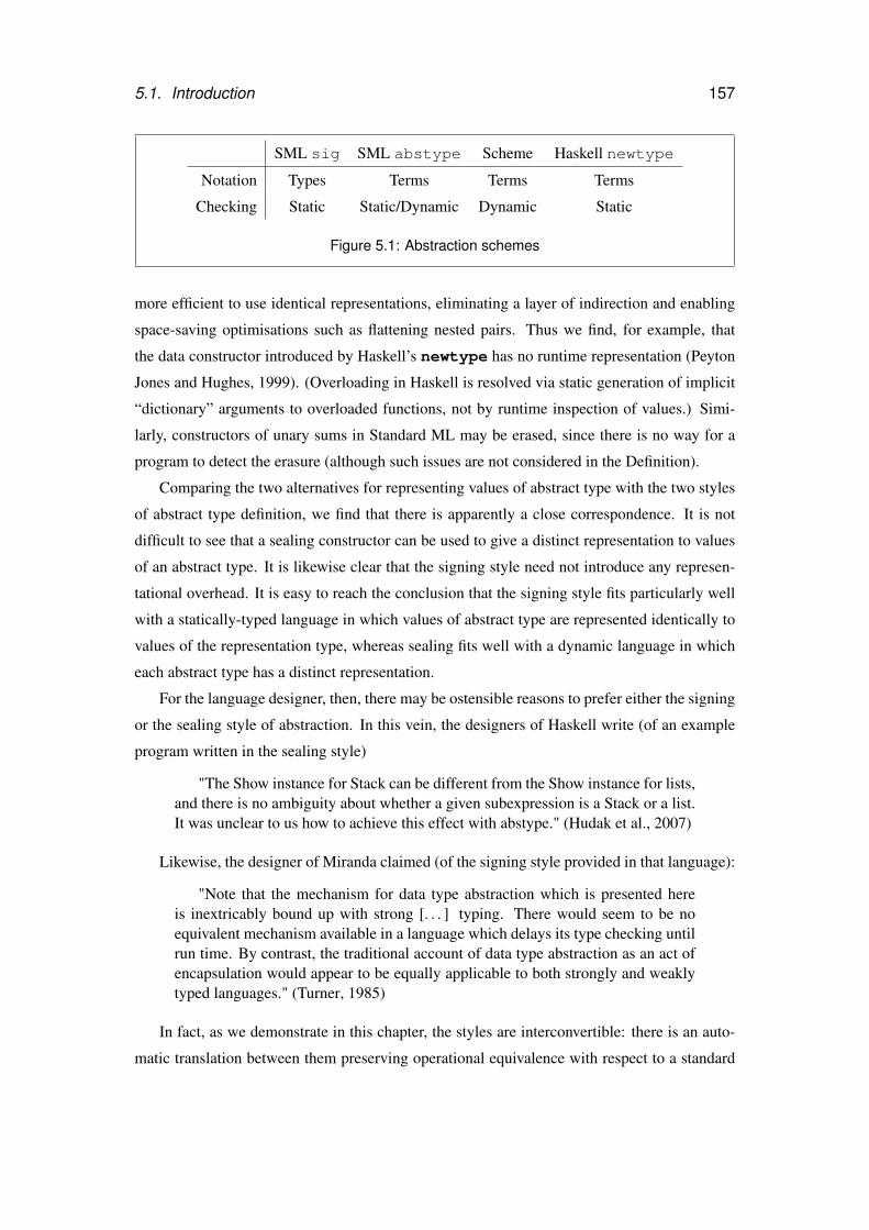
5.1. Introduction 157
SML sig SML abstype Scheme Haskell newtype
Notation Types Terms Terms Terms
Checking Static Static/Dynamic Dynamic Static
Figure 5.1: Abstraction schemes
more efficient to use identical representations, eliminating a layer of indirection and enabling
space-saving optimisations such as flattening nested pairs. Thus we find, for example, that
the data constructor introduced by Haskell’s newtype has no runtime representation (Peyton
Jones and Hughes, 1999). (Overloading in Haskell is resolved via static generation of implicit
“dictionary” arguments to overloaded functions, not by runtime inspection of values.) Simi-
larly, constructors of unary sums in Standard ML may be erased, since there is no way for a
program to detect the erasure (although such issues are not considered in the Definition).
Comparing the two alternatives for representing values of abstract type with the two styles
of abstract type definition, we find that there is apparently a close correspondence. It is not
difficult to see that a sealing constructor can be used to give a distinct representation to values
of an abstract type. It is likewise clear that the signing style need not introduce any represen-
tational overhead. It is easy to reach the conclusion that the signing style fits particularly well
with a statically-typed language in which values of abstract type are represented identically to
values of the representation type, whereas sealing fits well with a dynamic language in which
each abstract type has a distinct representation.
For the language designer, then, there may be ostensible reasons to prefer either the signing
or the sealing style of abstraction. In this vein, the designers of Haskell write (of an example
program written in the sealing style)
"The Show instance for Stack can be different from the Show instance for lists,and there is no ambiguity about whether a given subexpression is a Stack or a list.It was unclear to us how to achieve this effect with abstype." (Hudak et al., 2007)
Likewise, the designer of Miranda claimed (of the signing style provided in that language):
"Note that the mechanism for data type abstraction which is presented hereis inextricably bound up with strong [. . . ] typing. There would seem to be noequivalent mechanism available in a language which delays its type checking untilrun time. By contrast, the traditional account of data type abstraction as an act ofencapsulation would appear to be equally applicable to both strongly and weaklytyped languages." (Turner, 1985)
In fact, as we demonstrate in this chapter, the styles are interconvertible: there is an auto-
matic translation between them preserving operational equivalence with respect to a standard
158 Chapter 5. Signed and sealed
semantics. That is, we may define abstract types using either the signing or the sealing style
without constraining the runtime representation of values. For example, as we show in Sec-
tion 5.5, it is possible to extend Haskell with a construct for signing by translation into the
built-in constructs, thus avoiding the need for the user to write tags; we could equally well add
such a mechanism to Scheme. While it appeared to the Haskell designers that newtype was
necessary to avoid ambiguity in overloaded functions, it would, in fact, have been possible to
use a construct based on signing without any such ambiguity.
Early plans for this dissertation connected the discussion above more closely with the work
in Chapter 4. Generic functions, as discussed in that chapter, are closely connected to overload-
ing; functions such as eq and pickle (Sections 4.2.1 and 4.3) are overloaded for all algebraic
types (although the behaviour at each type is determined by the structure of the type rather than
specified in an ad-hoc fashion). As discussed above, overloading is, in turn, connected to ab-
stract types: an approach to overloading that depends on runtime inspection of values can only
offer different behaviour at an abstract type and its representation if the two are represented
differently at runtime. In this chapter we show that the representation of a value of abstract
type is not tied to the notation used for the definition of the type; we had hoped to build upon
this foundation to show that similar freedoms exist when designing systems of overloading and
generic programming, but time constraints ultimately prevented such an investigation.
Our evidence that the two styles of abstract type are interconvertible is based on relational
parametricity (Reynolds, 1983, Wadler, 1989). Pitts (2000) gives an appealing presentation
of parametricity in the presence of polymorphism and partial functions, in which the usual
denotational characterisation of admissible relations is replaced by a purely syntactic approach.
Our evidence is an application of the central result in a minor extension to Pitts’ system.
This chapter makes the following contributions:
1. A characterisation of the two essential styles of abstract type, signing and sealing (Sec-
tions 5.1 and 5.2.1).
2. Evidence that the two styles are interconvertible (Section 5.4) via a type-indexed function
(Section 5.3) in a higher-order language with polymorphism and recursion, based on an
extension of Pitts’ PolyPCF (Section 5.2).
3. An application of the result: a robust implementation of abstract types using signing to
Haskell (Section 5.5), by translation into Haskell’s sealing-style construct, newtype.
5.2. PolyPCF with tags 159
5.2 PolyPCF with tags
In order to demonstrate the equivalence of the two styles of defining abstract types we begin
by defining a programming language in which both styles can be expressed. Our language of
choice is an extension of Pitts’ PolyPCF (Pitts, 2000), which was designed to investigate the
operational behaviour of programs built from partial polymorphic functions. The signing style
of abstract type definition can be reduced to a use case of polymorphic types, already present
in PolyPCF. In order to capture the sealing style we extend PolyPCF with tags, a sort of unary
variant type with a constructor inT , destructor outT and type constructor T(−), for each T of
an infinite set of tag names Tag.
It is convenient to establish the necessary results in terms of polymorphic types and tag
types. The language constructs which we will ultimately use to compare signing and sealing
— signtype and sealtype — may be reduced to particular uses of these more primi-
tive constructs. Starting with polymorphism and tags simplifies both the initial presentation
of PolyPCF and the proofs. (One less desirable feature of this approach is that our simpler
language does not capture certain aspects of the signing and sealing styles, most notably the
scoping of tags that is essential to the sealing style. For the moment we emulate this scop-
ing by side conditions on the programs in which our abstract types are used, leaving a closer
emulation of the two styles to future work.)
We will first illustrate by example how abstract types may be defined in PolyPCF (Sec-
tion 5.2.1), then proceed to the formal development of the core language (Sections 5.2.2–
5.2.10). Section 5.4 gives the formal definition of the derived forms signtype and
sealtype.
5.2.1 Example
The four programs in Figure 5.2 illustrate the encoding of the two styles of type abstraction.
Our examples make use of types for pairs and numbers which are not directly supported by
PolyPCF, but which can be Church-encoded in the usual way (Girard, Taylor, and Lafont,
1989). We will use pairs and numbers as though PolyPCF supported them directly.
The program on the upper left gives a signing-style definition of a complex number type
using signtype. The program on the lower left gives the same definition written in plain
PolyPCF without signtype.
The program on the upper right gives a sealing-style definition of a complex number type
using sealtype. Since PolyPCF is explicitly typed — unlike, say, Standard ML — we must
give a type signature for each exported value. The program on the lower right gives the same
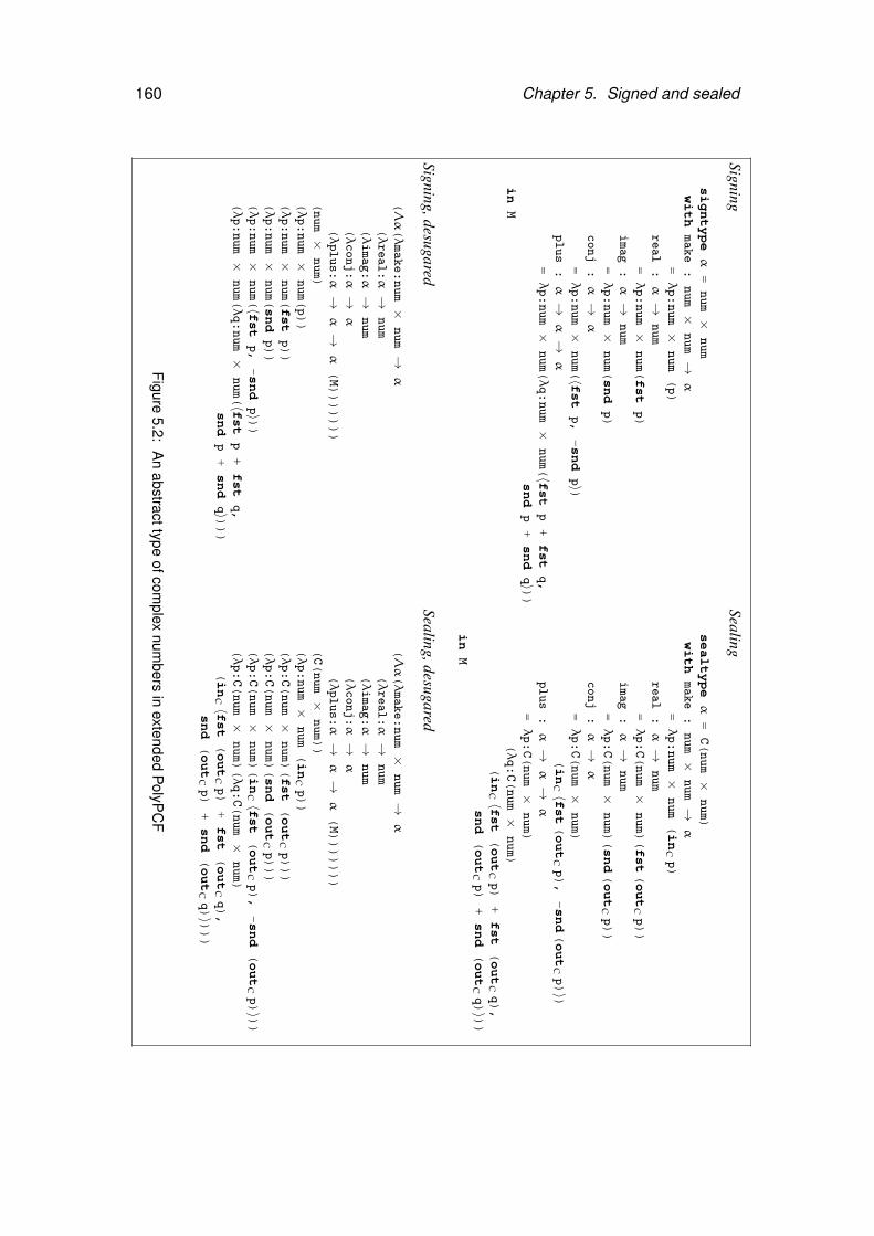
160 Chapter 5. Signed and sealed
Signing
signtypeα
=num×
num
with
make:
num×
num→
α
=λp:num×
num(p)
real:α→
num
=λp:num×
num(fst
p)
imag:α→
num
=λp:num×
num(snd
p)
conj:α→
α
=λp:num×
num(〈f
st
p,-snd
p〉)plus:α→
α→
α
=λp:num×
num(λq:num×
num(〈f
st
p+
fst
q,
snd
p+
snd
q〉))
in
M
Signing,desugared
(Λα(λmake:num×
num→
α
(λreal:α→
num
(λimag:α→
num
(λconj:α→
α
(λplus:α→
α→
α(M)))))))
(num×
num)
(λp:num×
num(p))
(λp:num×
num(fst
p))
(λp:num×
num(snd
p))
(λp:num×
num(〈f
st
p,-snd
p〉))
(λp:num×
num(λq:num×
num(〈f
st
p+
fst
q,
snd
p+
snd
q〉)))
Sealing
sealtypeα
=C(num×
num)
with
make:
num×
num→
α
=λp:num×
num(inCp)
real:α→
num
=λp:C(num×
num)(fst(outCp))
imag:α→
num
=λp:C(num×
num)(snd(outCp))
conj:α→
α
=λp:C(num×
num)
(inC〈fst(outCp),-snd(outCp)〉)
plus:α→
α→
α
=λp:C(num×
num)
(λq:C(num×
num)
(inC〈fst(outCp)+fst
(outCq),
snd
(outCp)+
snd(outCq)〉)
)in
M
Sealing,desugared
(Λα(λmake:num×
num→
α
(λreal:α→
num
(λimag:α→
num
(λconj:α→
α
(λplus:α→
α→
α(M)))))))
(C(num×
num))
(λp:num×
num(inCp))
(λp:C(num×
num)(fst(outCp)))
(λp:C(num×
num)(snd(outCp)))
(λp:C(num×
num)(inC〈fst(outCp),-snd(outCp)〉)
)(λp:C(num×
num)(λq:C(num×
num)
(inC〈fst
(outCp)+
fst(outCq),
snd(outCp)+snd(outCq)〉)
))
Figure5.2:
An
abstracttypeofcom
plexnum
bersin
extendedPolyP
CF
5.2. PolyPCF with tags 161
definition written in plain PolyPCF without sealtype.
The remainder of this section is a straightforward recapitulation of Pitts (2000). Most
figures and definitions are adapted from this work, the key difference being the addition of
tags. Adding tags is straightforward: no new insight or style of proof is required. The bracketed
numbers accompanying each definition and figure refer to the corresponding definition or figure
in Pitts’ work.
5.2.2 Syntax
Fig. 5.3 defines the syntax of our extension of PolyPCF. We follow standard conventions: for
example, application is left associative and we omit parentheses where possible.
PolyPCF augments the familiar polymorphic lambda calculus with fixpoint recursion and
polymorphic lists, which serve the role of a ground type. We add a type constructor, T(−), for
tagged types, and corresponding term constructors, inT - for tagging and outT - for untagging.
5.2.3 Typing
Figure 5.4 gives the typing relation Γ ` M : τ between typing environments Γ , terms M
and types τ. As the rules are entirely standard we refrain from commenting further.
5.2.4 Evaluation
Definition 27. (Values). The set V of values is drawn from the set of closed terms of closed
type generated by the following grammar:
V ::= λx : τ(M)
Λα(M)
nilτ
M ::M
inT M
Figure 5.5 gives the evaluation relation for extended PolyPCF. The rules are mostly deter-
mined by the definition of values. Function application is call-by-name.
5.2.5 Equivalence
In order to show that the two styles of creating abstract types are equivalent we must first make
clear what we mean by “equivalence” of terms. A common approach is to base equivalence on
the notion of context: two terms are considered equivalent if they may be interchanged in any
program context without effect on the observable behaviour of the program. This raises the
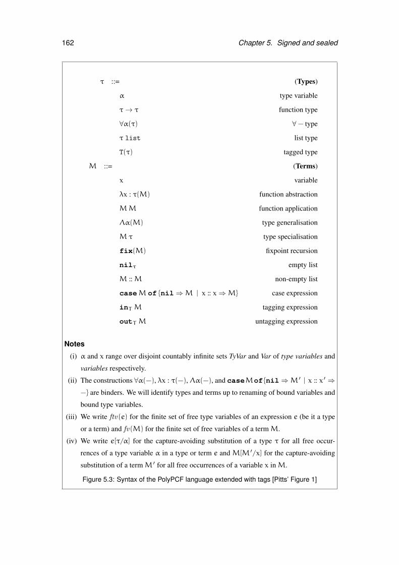
162 Chapter 5. Signed and sealed
τ ::= (Types)
α type variable
τ→ τ function type
∀α(τ) ∀− type
τ list list type
T(τ) tagged type
M ::= (Terms)
x variable
λx : τ(M) function abstraction
MM function application
Λα(M) type generalisation
Mτ type specialisation
fix(M) fixpoint recursion
nilτ empty list
M ::M non-empty list
caseM of {nil⇒M | x :: x⇒M} case expression
inT M tagging expression
outT M untagging expression
Notes
(i) α and x range over disjoint countably infinite sets TyVar and Var of type variables and
variables respectively.
(ii) The constructions ∀α(−), λx : τ(−),Λα(−), and caseMof {nil⇒M ′ | x :: x ′ ⇒−} are binders. We will identify types and terms up to renaming of bound variables and
bound type variables.
(iii) We write ftv(e) for the finite set of free type variables of an expression e (be it a type
or a term) and fv(M) for the finite set of free variables of a termM.
(iv) We write e[τ/α] for the capture-avoiding substitution of a type τ for all free occur-
rences of a type variable α in a type or term e and M[M ′/x] for the capture-avoiding
substitution of a termM ′ for all free occurrences of a variable x inM.
Figure 5.3: Syntax of the PolyPCF language extended with tags [Pitts’ Figure 1]

5.2. PolyPCF with tags 163
Γ , x : τ ` x : τ
Γ , x : τ1 `M : τ2
Γ ` λx : τ1(M) : τ1 → τ2
Γ ` F : τ1 → τ2 Γ ` A : τ1
Γ ` F A : τ2
Γ ,α `M : τ
Γ ` Λα(M) : ∀α(τ)
Γ ` G : ∀α(τ1)
Γ ` G τ2 : τ1[τ2/α]
Γ ` F : τ→ τ
Γ ` fix(F) : τ
Γ ` nilτ : τ list Γ ` H : τ Γ ` T : τ list
Γ ` H :: T : τ list
Γ ` L : τ1 list Γ `M1 : τ2 Γ ,h : τ1, t : τ1 list `M2 : τ2
Γ ` case L of {nil⇒M1 | h :: t⇒M2} : τ2
Γ `M : τ
Γ ` inT M : T(τ)
Γ `M : T(τ)
Γ ` outT M : τ
Notes
(i) Typing judgments take the form Γ `M : τ where
(a) the typing environment Γ is a pair A,∆ with A a finite subset of TyVar and ∆ a
function defined on a finite subset dom(∆) of Var and mapping each x ∈ dom(∆)
to a type with free type variables in A;
(b) M is a term with ftv(M) ⊆ A and fv(M) ⊆ dom(∆);
(c) τ is a type with ftv(τ) ⊆ A.
(ii) The notation Γ , x : τ indicates the typing environment obtained from the typing envi-
ronment Γ = A,∆ by properly extending the function ∆ by mapping x /∈ dom(∆) to
τ. Similarly, Γ ,α is the typing environment obtained by properly extending A with an
α /∈ A.
(iii) The explicit type information included in the syntax of function abstractions and empty
lists ensures that, given Γ andM, there is at most one τ for which Γ `M : τ holds.
Figure 5.4: Typing assignment relation for PolyPCF with tags [Pitts’ Figure 2]
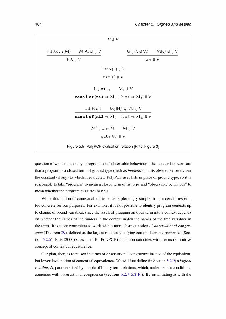
164 Chapter 5. Signed and sealed
V ⇓ V
F ⇓ λx : τ(M) M[A/x] ⇓ V
F A ⇓ V
G ⇓ Λα(M) M[τ/α] ⇓ V
G τ ⇓ V
F fix(F) ⇓ V
fix(F) ⇓ V
L ⇓ nilτ M1 ⇓ V
case L of {nil⇒M1 | h :: t⇒M2} ⇓ V
L ⇓ H :: T M2[H/h, T/t] ⇓ V
case L of {nil⇒M1 | h :: t⇒M2} ⇓ V
M ′ ⇓ inT M M ⇓ V
outT M ′ ⇓ V
Figure 5.5: PolyPCF evaluation relation [Pitts’ Figure 3]
question of what is meant by “program” and “observable behaviour”; the standard answers are
that a program is a closed term of ground type (such as boolean) and its observable behaviour
the constant (if any) to which it evaluates. PolyPCF uses lists in place of ground type, so it is
reasonable to take “program” to mean a closed term of list type and “observable behaviour” to
mean whether the program evaluates to nil.
While this notion of contextual equivalence is pleasingly simple, it is in certain respects
too concrete for our purposes. For example, it is not possible to identify program contexts up
to change of bound variables, since the result of plugging an open term into a context depends
on whether the names of the binders in the context match the names of the free variables in
the term. It is more convenient to work with a more abstract notion of observational congru-
ence (Theorem 29), defined as the largest relation satisfying certain desirable properties (Sec-
tion 5.2.6). Pitts (2000) shows that for PolyPCF this notion coincides with the more intuitive
concept of contextual equivalence.
Our plan, then, is to reason in terms of observational congruence instead of the equivalent,
but lower-level notion of contextual equivalence. We will first define (in Section 5.2.9) a logical
relation, ∆, parameterised by a tuple of binary term relations, which, under certain conditions,
coincides with observational congruence (Sections 5.2.7–5.2.10). By instantiating ∆ with the
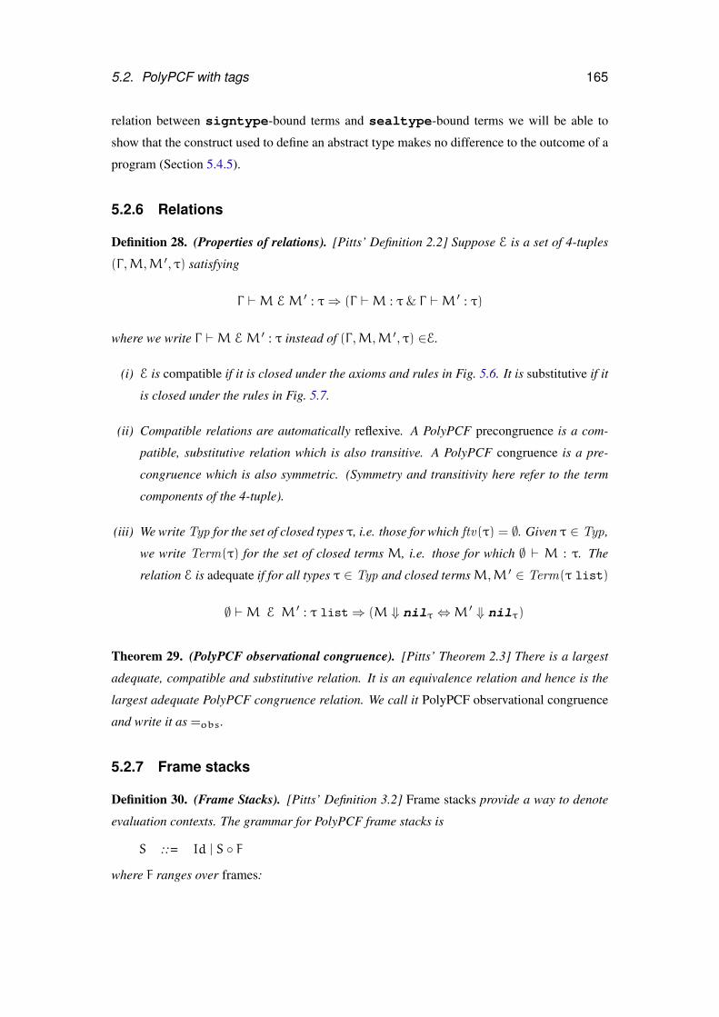
5.2. PolyPCF with tags 165
relation between signtype-bound terms and sealtype-bound terms we will be able to
show that the construct used to define an abstract type makes no difference to the outcome of a
program (Section 5.4.5).
5.2.6 Relations
Definition 28. (Properties of relations). [Pitts’ Definition 2.2] Suppose E is a set of 4-tuples
(Γ ,M,M ′, τ) satisfying
Γ `M EM ′ : τ⇒ (Γ `M : τ& Γ `M ′ : τ)
where we write Γ `M EM ′ : τ instead of (Γ ,M,M ′, τ) ∈E.
(i) E is compatible if it is closed under the axioms and rules in Fig. 5.6. It is substitutive if it
is closed under the rules in Fig. 5.7.
(ii) Compatible relations are automatically reflexive. A PolyPCF precongruence is a com-
patible, substitutive relation which is also transitive. A PolyPCF congruence is a pre-
congruence which is also symmetric. (Symmetry and transitivity here refer to the term
components of the 4-tuple).
(iii) We write Typ for the set of closed types τ, i.e. those for which ftv(τ) = ∅. Given τ ∈ Typ,
we write Term(τ) for the set of closed terms M, i.e. those for which ∅ ` M : τ. The
relation E is adequate if for all types τ ∈ Typ and closed termsM,M ′ ∈ Term(τ list)
∅ `M E M ′ : τ list⇒ (M ⇓ nilτ ⇔M ′ ⇓ nilτ)
Theorem 29. (PolyPCF observational congruence). [Pitts’ Theorem 2.3] There is a largest
adequate, compatible and substitutive relation. It is an equivalence relation and hence is the
largest adequate PolyPCF congruence relation. We call it PolyPCF observational congruence
and write it as =obs.
5.2.7 Frame stacks
Definition 30. (Frame Stacks). [Pitts’ Definition 3.2] Frame stacks provide a way to denote
evaluation contexts. The grammar for PolyPCF frame stacks is
S ::= Id | S ◦ F
where F ranges over frames:
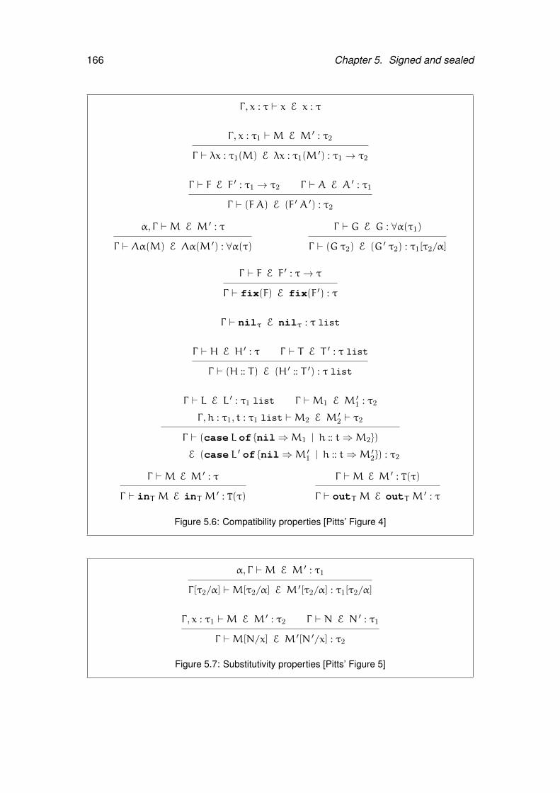
166 Chapter 5. Signed and sealed
Γ , x : τ ` x E x : τ
Γ , x : τ1 `M E M ′ : τ2
Γ ` λx : τ1(M) E λx : τ1(M′) : τ1 → τ2
Γ ` F E F ′ : τ1 → τ2 Γ ` A E A ′ : τ1
Γ ` (F A) E (F ′ A ′) : τ2
α, Γ `M E M ′ : τ
Γ ` Λα(M) E Λα(M ′) : ∀α(τ)
Γ ` G E G : ∀α(τ1)
Γ ` (G τ2) E (G ′ τ2) : τ1[τ2/α]
Γ ` F E F ′ : τ→ τ
Γ ` fix(F) E fix(F ′) : τ
Γ ` nilτ E nilτ : τ list
Γ ` H E H ′ : τ Γ ` T E T ′ : τ list
Γ ` (H :: T) E (H ′ :: T ′) : τ list
Γ ` L E L ′ : τ1 list Γ `M1 E M ′1 : τ2
Γ ,h : τ1, t : τ1 list `M2 E M ′2 ` τ2
Γ ` (case L of {nil⇒M1 | h :: t⇒M2})
E (case L ′ of {nil⇒M ′1 | h :: t⇒M ′2}) : τ2
Γ `M E M ′ : τ
Γ ` inT M E inT M ′ : T(τ)
Γ `M E M ′ : T(τ)
Γ ` outT M E outT M ′ : τ
Figure 5.6: Compatibility properties [Pitts’ Figure 4]
α, Γ `M E M ′ : τ1
Γ [τ2/α] `M[τ2/α] E M ′[τ2/α] : τ1[τ2/α]
Γ , x : τ1 `M E M ′ : τ2 Γ ` N E N ′ : τ1
Γ `M[N/x] E M ′[N ′/x] : τ2
Figure 5.7: Substitutivity properties [Pitts’ Figure 5]
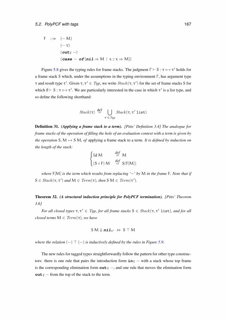
5.2. PolyPCF with tags 167
F ::= (−M)
(− τ)
(outT −)
(case − of {nil⇒M | x :: x⇒M})
Figure 5.8 gives the typing rules for frame stacks. The judgment Γ ` S : τ ◦→ τ ′ holds for
a frame stack S which, under the assumptions in the typing environment Γ , has argument type
τ and result type τ ′. Given τ, τ ′ ∈ Typ, we write Stack(τ, τ ′) for the set of frame stacks S for
which ∅ ` S : τ ◦→ τ ′. We are particularly interested in the case in which τ ′ is a list type, and
so define the following shorthand:
Stack(τ)def=
⋃τ ′∈Typ
Stack(τ, τ ′ list)
Definition 31. (Applying a frame stack to a term). [Pitts’ Definition 3.4] The analogue for
frame stacks of the operation of filling the hole of an evaluation context with a term is given by
the operation S,M 7→ SM, of applying a frame stack to a term. It is defined by induction on
the length of the stack: IdMdef= M
(S ◦ F)M def= S(F[M])
where F[M] is the term which results from replacing ‘−’ by M in the frame F. Note that if
S ∈ Stack(τ, τ ′) andM ∈ Term(τ), then SM ∈ Term(τ ′).
Theorem 32. (A structural induction principle for PolyPCF termination). [Pitts’ Theorem
3.6]
For all closed types τ, τ ′ ∈ Typ, for all frame stacks S ∈ Stack(τ, τ ′ list), and for all
closed termsM ∈ Term(τ), we have
SM ⇓ nilτ ′ ⇔ S >M
where the relation (−) > (−) is inductively defined by the rules in Figure 5.9.
The new rules for tagged types straightforwardly follow the pattern for other type construc-
tors: there is one rule that pairs the introduction form inT − with a stack whose top frame
is the corresponding elimination form outT −, and one rule that moves the elimination form
outT − from the top of the stack to the term.
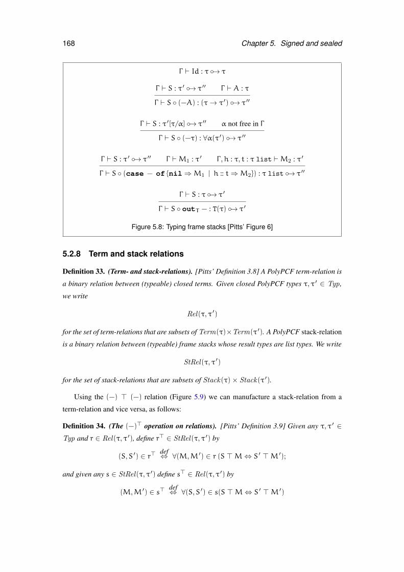
168 Chapter 5. Signed and sealed
Γ ` Id : τ ◦→ τ
Γ ` S : τ ′ ◦→ τ ′′ Γ ` A : τ
Γ ` S ◦ (−A) : (τ→ τ ′) ◦→ τ ′′
Γ ` S : τ ′[τ/α] ◦→ τ ′′ α not free in Γ
Γ ` S ◦ (−τ) : ∀α(τ ′) ◦→ τ ′′
Γ ` S : τ ′ ◦→ τ ′′ Γ `M1 : τ ′ Γ ,h : τ, t : τ list `M2 : τ ′
Γ ` S ◦ (case − of {nil⇒M1 | h :: t⇒M2}) : τ list ◦→ τ ′′
Γ ` S : τ ◦→ τ ′
Γ ` S ◦ outT − : T(τ) ◦→ τ ′
Figure 5.8: Typing frame stacks [Pitts’ Figure 6]
5.2.8 Term and stack relations
Definition 33. (Term- and stack-relations). [Pitts’ Definition 3.8] A PolyPCF term-relation is
a binary relation between (typeable) closed terms. Given closed PolyPCF types τ, τ ′ ∈ Typ,
we write
Rel(τ, τ ′)
for the set of term-relations that are subsets of Term(τ)×Term(τ ′). A PolyPCF stack-relation
is a binary relation between (typeable) frame stacks whose result types are list types. We write
StRel(τ, τ ′)
for the set of stack-relations that are subsets of Stack(τ)× Stack(τ ′).
Using the (−) > (−) relation (Figure 5.9) we can manufacture a stack-relation from a
term-relation and vice versa, as follows:
Definition 34. (The (−)> operation on relations). [Pitts’ Definition 3.9] Given any τ, τ ′ ∈Typ and r ∈ Rel(τ, τ ′), define r> ∈ StRel(τ, τ ′) by
(S,S ′) ∈ r> def⇔ ∀(M,M ′) ∈ r (S >M⇔ S ′ >M ′);
and given any s ∈ StRel(τ, τ ′) define s> ∈ Rel(τ, τ ′) by
(M,M ′) ∈ s> def⇔ ∀(S,S ′) ∈ s(S >M⇔ S ′ >M ′)
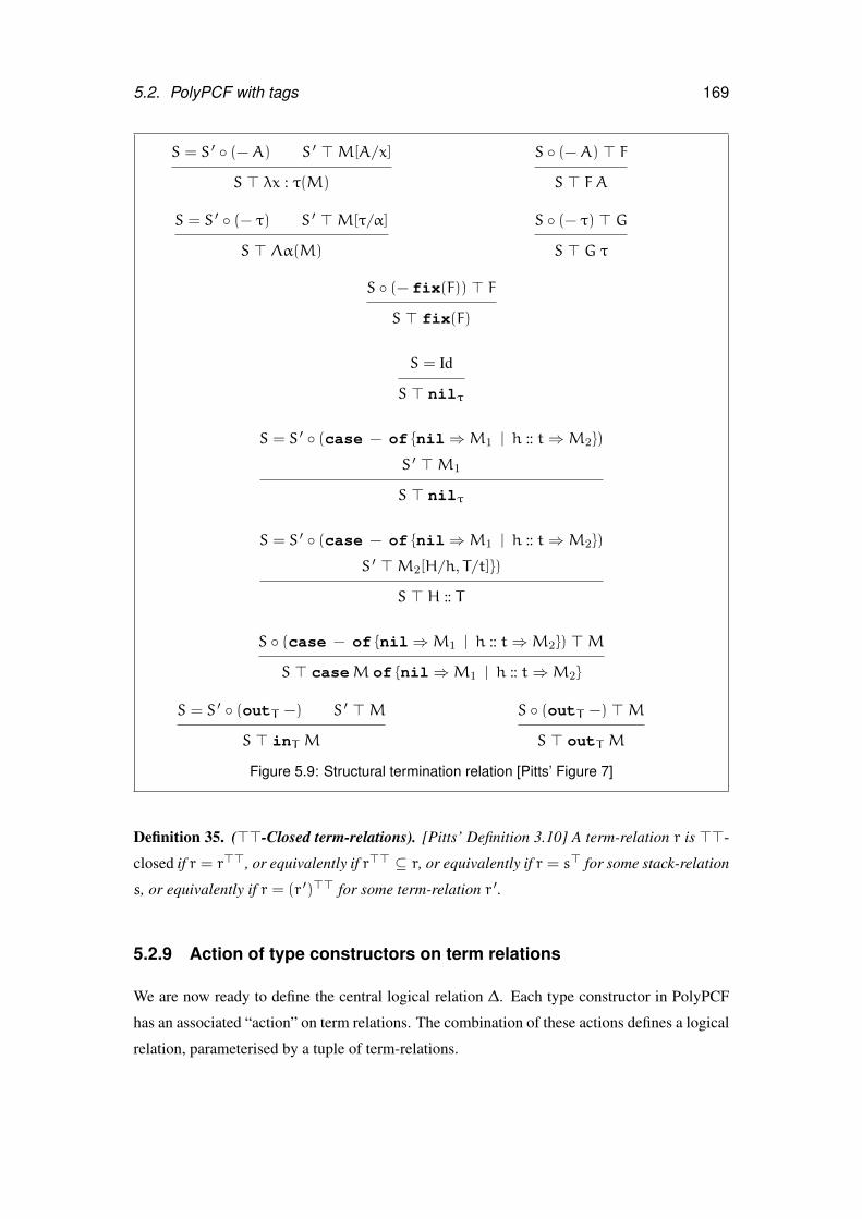
5.2. PolyPCF with tags 169
S = S ′ ◦ (−A) S ′ >M[A/x]
S > λx : τ(M)
S ◦ (−A) > F
S > F A
S = S ′ ◦ (− τ) S ′ >M[τ/α]
S > Λα(M)
S ◦ (− τ) > G
S > G τ
S ◦ (− fix(F)) > F
S > fix(F)
S = Id
S > nilτ
S = S ′ ◦ (case − of {nil⇒M1 | h :: t⇒M2})
S ′ >M1
S > nilτ
S = S ′ ◦ (case − of {nil⇒M1 | h :: t⇒M2})
S ′ >M2[H/h, T/t]})
S > H :: T
S ◦ (case − of {nil⇒M1 | h :: t⇒M2}) >M
S > caseM of {nil⇒M1 | h :: t⇒M2}
S = S ′ ◦ (outT −) S ′ >M
S > inT M
S ◦ (outT −) >M
S > outT M
Figure 5.9: Structural termination relation [Pitts’ Figure 7]
Definition 35. (>>-Closed term-relations). [Pitts’ Definition 3.10] A term-relation r is >>-
closed if r = r>>, or equivalently if r>> ⊆ r, or equivalently if r = s> for some stack-relation
s, or equivalently if r = (r ′)>> for some term-relation r ′.
5.2.9 Action of type constructors on term relations
We are now ready to define the central logical relation ∆. Each type constructor in PolyPCF
has an associated “action” on term relations. The combination of these actions defines a logical
relation, parameterised by a tuple of term-relations.
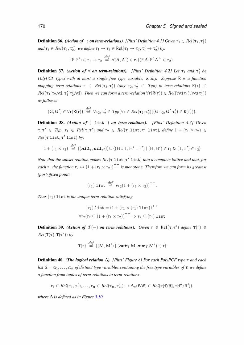
170 Chapter 5. Signed and sealed
Definition 36. (Action of→ on term-relations). [Pitts’ Definition 4.1] Given r1 ∈ Rel(τ1, τ ′1)
and r2 ∈ Rel(τ2, τ ′2), we define r1 → r2 ∈ Rel(τ1 → τ2, τ ′1 → τ ′2) by:
(F, F ′) ∈ r1 → r2def⇔ ∀(A,A ′) ∈ r1((F A, F ′ A ′) ∈ r2).
Definition 37. (Action of ∀ on term-relations). [Pitts’ Definition 4.2] Let τ1 and τ ′1 be
PolyPCF types with at most a single free type variable, α say. Suppose R is a function
mapping term-relations r ∈ Rel(τ2, τ ′2) (any τ2, τ ′2 ∈ Typ) to term-relations R(r) ∈Rel(τ1[τ2/α], τ
′1[τ′2/α]). Then we can form a term-relation ∀r(R(r)) ∈ Rel(∀α(τ1), ∀α(τ ′1))
as follows:
(G,G ′) ∈ ∀r(R(r)) def⇔ ∀τ2, τ ′2 ∈ Typ(∀r ∈ Rel(τ2, τ ′2)((G τ2,G ′ τ ′2) ∈ R(r))).
Definition 38. (Action of ( list−) on term-relations). [Pitts’ Definition 4.3] Given
τ, τ ′ ∈ Typ, r1 ∈ Rel(τ, τ ′) and r2 ∈ Rel(τ list, τ ′ list), define 1 + (r1 × r2) ∈Rel(τ list, τ ′ list) by:
1 + (r1 × r2)def= {(nilτ,nilτ ′)} ∪ {(H :: T ,H ′ :: T ′) | (H,H ′) ∈ r1 & (T , T ′) ∈ r2}
Note that the subset relation makes Rel(τ list, τ ′ list) into a complete lattice and that, for
each r1 the function r2 7→ (1 + (r1 × r2))>> is monotone. Therefore we can form its greatest
(post-)fixed point:
(r1) listdef= νr2(1 + (r1 × r2))>>.
Thus (r1) list is the unique term-relation satisfying
(r1) list = (1 + (r1 × (r1) list))>>
∀r2(r2 ⊆ (1 + (r1 × r2))>> ⇒ r2 ⊆ (r1) list
Definition 39. (Action of T (−) on term relations). Given r ∈ Rel(τ, τ ′) define T(r) ∈Rel(T(τ), T(τ ′)) by
T(r)def= {(M,M ′) | (outT M,outT M
′) ∈ r}
Definition 40. (The logical relation ∆). [Pitts’ Figure 8] For each PolyPCF type τ and each
list ~α = α1, . . . ,αn of distinct type variables containing the free type variables of τ, we define
a function from tuples of term-relations to term-relations
r1 ∈ Rel(τ1, τ ′1), . . . , rn ∈ Rel(τn, τ ′n) 7→ ∆τ(~r/~α) ∈ Rel(τ[~τ/~α], τ[~τ ′/~α ′]).
where ∆ is defined as in Figure 5.10.
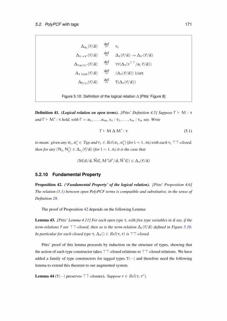
5.2. PolyPCF with tags 171
∆αi(~r/~α)def= ri
∆τ→τ ′(~r/~α)def= ∆τ(~r/~α)→ ∆τ ′(~r/~α)
∆∀α(τ) ′(~r/~α)def= ∀r(∆τ(r>>/α,~r/~α))
∆τ list(~r/~α)def= (∆τ(~r/~α)) list
∆T(τ)(~r/~α)def= T(∆τ(~r/~α))
Figure 5.10: Definition of the logical relation ∆ [Pitts’ Figure 8]
Definition 41. (Logical relation on open terms). [Pitts’ Definition 4.5] Suppose Γ ` M : τ
and Γ `M ′ : τ hold, with Γ = α1, . . . ,αm, x1 : τ1, . . . , xn : τn say. Write
Γ `M ∆M ′ : τ (5.1)
to mean: given any σi,σ ′i ∈ Typ and ri ∈ Rel(σi,σ′i) (for i = 1..m) with each ri >>-closed,
then for any (Nj,N′j) ∈ ∆rj(~r/~α) (for i = 1..n) it is the case that
(M[~σ/~α, ~N~x],M ′[~σ ′/~α, ~N ′~x]) ∈ ∆τ(~r/~α)
5.2.10 Fundamental Property
Proposition 42. (‘Fundamental Property’ of the logical relation). [Pitts’ Proposition 4.6]
The relation (5.1) between open PolyPCF terms is compatible and substitutive, in the sense of
Definition 28.
The proof of Proposition 42 depends on the following Lemma:
Lemma 43. [Pitts’ Lemma 4.11] For each open type τ, with free type variables in ~α say, if the
term-relations ~r are >>-closed, then so is the term-relation ∆r(~r/~α) defined in Figure 5.10.
In particular for each closed type τ, ∆τ() ∈ Rel(τ, τ) is >>-closed.
Pitts’ proof of this lemma proceeds by induction on the structure of types, showing that
the action of each type constructor takes >>-closed relations to >>-closed relations. We have
added a family of type constructors for tagged types T(−) and therefore need the following
lemma to extend this theorem to our augmented system.
Lemma 44 (T(−) preserves >>-closure). Suppose r ∈ Rel(τ, τ ′).
172 Chapter 5. Signed and sealed
(i) Suppose given values inTM and inTM ′ of types T(τ) and T(τ ′) respectively, satisfying
(M,M ′) ∈ r.
If r is >>-closed then (inT M,inT M ′) ∈ T(r).
(ii) If (S,S ′) ∈ r> then (S ◦ outT −,S ′ ◦ outT −) ∈ T(r)>.
(iii) If r is >>-closed then so is T(r).
Proof.
(i) The statement in (i) follows from the equivalence
outT inT M ⇓ V ⇐⇒ M ⇓ V
(ii) Suppose (S,S ′) ∈ r>. For any (N,N ′) ∈ T(r) we have
S ◦ outT − > N ⇔ S > outT N
(by definition of (−) > (−))
⇔ S ′ > outT N ′
(since (outT N,outT N ′) ∈ rand (S,S ′) ∈ r>)
⇔ S ′ ◦ outT − > N ′
( by definition of (−) > (−))
It follows that (S ◦ outT −,S ′ ◦ outT −) ∈ T(r)>.
(iii) Suppose (S,S ′) ∈ r>, (N,N ′) ∈ r, (M,M ′) ∈ T(r)>>. We must show that (M,M ′) ∈T(r).
By (ii) we have (S ◦ outT −,S ′ ◦ outT −) ∈ T(r)>, and hence
S ◦ outT − >M ⇔ S ′ ◦ outT − >M ′
Therefore
S > outT M ⇔ S ′ > outT M′
Thus, by the definition of (−)>, (outT M,outT M ′) ∈ (r>)> = r, and so (M,M ′) ∈T(r) by the definition of T(−). It follows that T(r) is >>-closed.
5.3. Tagging and untagging 173
Theorem 45. [Pitts’ Theorem 4.15] The logical relation (5.1) coincides with PolyPCF obser-
vational congruence:
Γ `M obs= M ′ : τ ⇔ Γ `M ∆M ′ : τ (5.2)
Having established the necessary preliminaries to the equivalence proof, we now turn to
the development of the conversion between the two styles of abstract type.
5.3 Tagging and untagging
5.3.1 Example
The conversion between signing-style and sealing-style definitions of abstract types is per-
formed by a pair of type-indexed functions which insert and remove tags as necessary. For
example, to convert the function plus in the signing-style implementation of the complex type
given in Section 5.2.1 into a function that can be used in the sealing-style implementation we
generate a function of type
(α→ α→ α)→ (C(α)→ C(α)→ C(α))
where α is the type variable denoting the abstract type of complex numbers and C is the tag
used in the sealed representation. The conversion function generated for the type of plus in
the sealed representation is
λh:α→α→α(λx:C(α)((λj:α→α(λy:C(α)((λz:α(inC z)) (j ((λz:C(α)(outC z)) y)))))(h ((λz:C(α)(outC z)) x))))
which, after the “administrative” redexes introduced by the generation function are reduced,
becomes
λh : (α→ α→ α)(λx : C(α) (λy : C(α) (inC (h (outC x) (outC y)))))
Conversely, moving from the sealed to the signed representation requires a function of type
(C(α)→ C(α)→ C(α))→ (α→ α→ α)
In this case the generated term, after administrative reductions, is
λh : (C(α)→ C(α)→ C(α))(λx : α (λy : α (outC (h (inC x) (inC y)))))
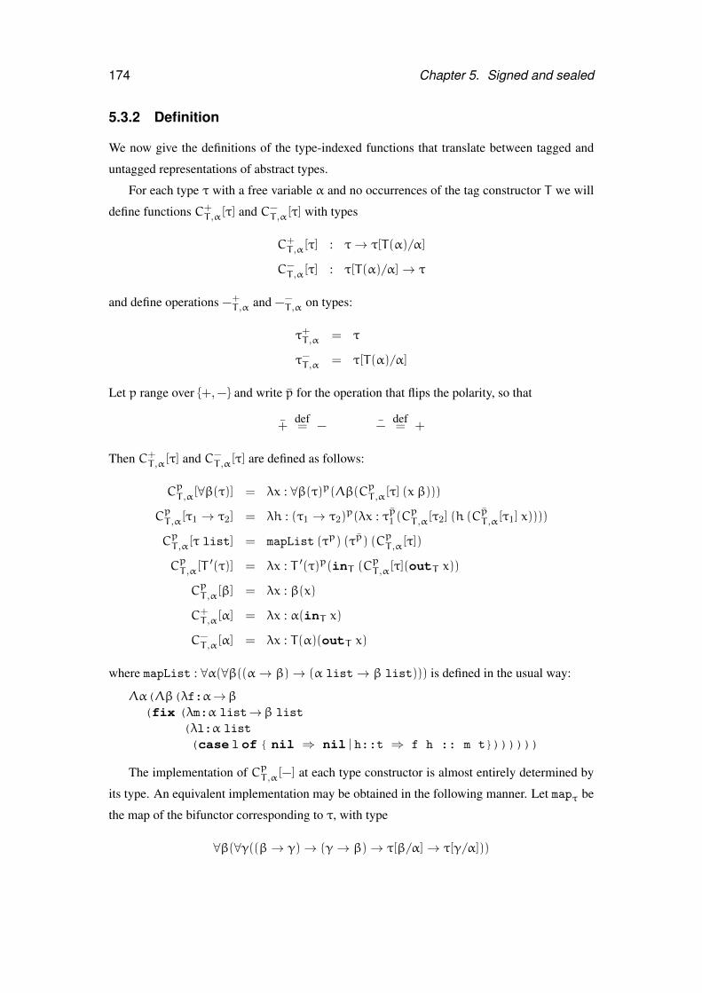
174 Chapter 5. Signed and sealed
5.3.2 Definition
We now give the definitions of the type-indexed functions that translate between tagged and
untagged representations of abstract types.
For each type τ with a free variable α and no occurrences of the tag constructor T we will
define functions C+T ,α[τ] and C−
T ,α[τ] with types
C+T ,α[τ] : τ→ τ[T(α)/α]
C−T ,α[τ] : τ[T(α)/α]→ τ
and define operations −+T ,α and −−
T ,α on types:
τ+T ,α = τ
τ−T ,α = τ[T(α)/α]
Let p range over {+,−} and write p̄ for the operation that flips the polarity, so that
+̄def= − −̄
def= +
Then C+T ,α[τ] and C−
T ,α[τ] are defined as follows:
CpT ,α[∀β(τ)] = λx : ∀β(τ)p(Λβ(CpT ,α[τ] (x β)))
CpT ,α[τ1 → τ2] = λh : (τ1 → τ2)
p(λx : τp̄1 (CpT ,α[τ2] (h (Cp̄T ,α[τ1] x))))
CpT ,α[τ list] = mapList (τp) (τp̄) (CpT ,α[τ])
CpT ,α[T
′(τ)] = λx : T ′(τ)p(inT (CpT ,α[τ](outT x))
CpT ,α[β] = λx : β(x)
C+T ,α[α] = λx : α(inT x)
C−T ,α[α] = λx : T(α)(outT x)
where mapList : ∀α(∀β((α→ β)→ (α list→ β list))) is defined in the usual way:
Λα(Λβ(λf:α→β(fix (λm:α list→β list
(λl:α list
(case l of { nil ⇒ nil | h::t ⇒ f h :: m t}))))))
The implementation of CpT ,α[−] at each type constructor is almost entirely determined by
its type. An equivalent implementation may be obtained in the following manner. Let mapτ be
the map of the bifunctor corresponding to τ, with type
∀β(∀γ((β→ γ)→ (γ→ β)→ τ[β/α]→ τ[γ/α]))
5.4. Signing and sealing 175
(In general, if τ has n free type variables, mapτ will take 2n functions, since each type variable
may occur positively or negatively in τ). Let inT ,α and outT ,α be defined as follows.
inT ,αdef= λx : α(inT x)
outT ,αdef= λx : T(α)(outT x)
Then
C+T ,α[τ]
def= λx : τ+T ,α(mapτ α (T(α)) inT ,α outT ,α)
C−T ,α[τ]
def= λx : τ−T .α(mapτ (T(α)) α outT ,α inT ,α)
Proposition 46. The functions C−T ,α[τ] and C+
T ,α[τ] are mutual inverses. That is, for all M of
type τ andM ′ of type T(τ),
C−T ,α[τ] (C
+T ,α[τ]M)
obs= M (5.3)
C+T ,α[τ] (C
−T ,α[τ]M
′)obs= M ′ (5.4)
Proof. Either directly using the standard β- and η- equalities that follow from the evaluation
rules, or indirectly via map fusion.
5.4 Signing and sealing
In Section 5.2.1 we introduced the constructs sealtype and signtype for creating abstract
types. We now give formal definitions of each construct, both directly and via desugaring into
the core language.
5.4.1 Syntax
M ::= . . .
| signtype α = τ with x1 : τ1 =M1 . . . xn : τn =Mn inM
| sealtype α = T(τ) with x1 : τ1 =M1 . . . xn : τn =Mn inM
As we noted in the introduction, the distinction between the two constructs is somewhat
obscured in PolyPCF by the need to supply type signatures for each exported component in both
the signtype and sealtype variants. In a language with type inference the signatures can
be omitted in sealtype definitions.
176 Chapter 5. Signed and sealed
5.4.2 Typing
The typing rules for signtype and sealtype are as follows.
Γ `Mi : τi[τ/α] (∀i.1 6 i 6 n)Γ ,α, x1 : τ1, . . . , xn : τn `M : τ ′ α /∈ fv(τ ′)
Γ ` signtype α = τ with x1 : τ1 =M1 . . . xn : τn :Mn inM : τ ′
Γ `Mi : τi[T(τ)/α] (∀i.1 6 i 6 n)Γ ,α, x1 : τ1, . . . , xn : τn `M : τ ′ α /∈ fv(τ ′)
Γ ` sealtype α = T(τ) with x1 : τ1 =M1 . . . xn : τn :Mn inM : τ ′
We associate two types with each of the fields xi of the interface of an abstract type defined
with signtype or sealtype. The first is the type τi ascribed to that field in the signature;
this is the type given to xi within the continuationM. The second is the concrete type, in which
every occurrence of the abstract type variable α has been replaced by the representation type:
that is, with τ for signtype and with T(τ) for sealtype. This concrete type must match
the type of the termMi that is bound to the field.
The hypotheses for each rule further specify that each of the fields of the interface is in
scope only within the continuation,M, and not within the terms bound to the other fields. This
is perhaps too restrictive for practical use, but it is a restriction that is easily overcome with
a further layer of sugar. We can obtain mutually-recursive definitions using an n-ary fixpoint
combinator for any signature of n operations. For example, a combinator for creating two
mutually recursive functions may be defined, rather impenetrably, as follows:
fix2 : ∀α(∀β(∀γ(∀δ((((α→β × γ→ δ) → α→β)× ((α→β × γ→ δ) → γ→ δ))→ (α→β × γ→ δ)))))
fix2 = Λα(Λβ(Λγ(Λδ(fix(λfix2:((((α→β × γ→ δ) → α→β)
× ((α→β × γ→ δ) → γ→ δ))→ (α→β × γ→ δ))→ ((((α→β × γ→ δ) → α→β)× ((α→β × γ→ δ) → γ→ δ))→ (α→β × γ→ δ))
(λfs:((α→β × γ→ δ) → α→β)× ((α→β × γ→ δ) → γ→ δ)
(〈λx:α((fst fs) (fix2 fs) x),λx:γ((snd fs) (fix2 fs) x)〉)))))))
5.4. Signing and sealing 177
5.4.3 Evaluation
The evaluation rules for signtype and sealtype are as follows.
M[τ/α,M1/x1, . . .Mn/xn] ⇓ V
signtype α = τ with x1 : τ1 =M1 . . . xn : τn :Mn inM ⇓ V
M[T(τ)/α,M1/x1, . . .Mn/xn] ⇓ V
sealtype α = T(τ) with x1 : τ1 =M1 . . . xn : τn :Mn inM ⇓ V
Evaluation is straightforward: the continuation M is evaluated after substituting the ab-
stract type T(τ) or τ for the abstract type variable α and the fields M1 . . .Mn for the corre-
sponding variables xi . . . xn. Like PolyPCF function application, evaluation of the signtype
and sealtype constructs is call-by-name.
5.4.4 Desugaring
Both signtype and sealtype are derived forms; there is a straightforward translation into
core PolyPCF terms, as shown by the following lemma.
Lemma 47 (Desugaring). Let I, J, K and L be defined as follows for some non-negative integer
n, termsM,M1, . . .Mn and types τ, τ1, . . . τn.
Idef= signtype α = τ with x1 : τ1 =M1 . . . xn : τn :Mn inM
Jdef= sealtype α = T(τ) with x1 : τ1 =M1 . . . xn : τn :Mn inM
Kdef= (Λα(λx1 : τ1(. . . λxn : τn(M)) . . .)) (τ)M1 . . . Mn
Ldef= (Λα(λx1 : τ1(. . . λxn : τn(M)) . . .)) (T(τ))M1 . . . Mn
Then the following hold:
Γ ` I : τ ′ ⇐⇒ Γ ` K : τ ′ (5.5)
Γ ` J : τ ′ ⇐⇒ Γ ` L : τ ′ (5.6)
I ⇓ V ⇐⇒ K ⇓ V (5.7)
J ⇓ V ⇐⇒ L ⇓ V (5.8)
where α /∈ fv(τ ′).
178 Chapter 5. Signed and sealed
Proof. The statements 5.5 and 5.6 follow directly from the definition of the typing relation
` : in Section 5.4.2 and Figure 5.4.
The statements 5.7 and 5.8 follow directly from the definition of the evaluation relation ⇓in Section 5.4.3 and Figure 5.5.
It is more conventional to present abstract types in terms of existential types (Pierce, 2002,
Chapter 24) than universal types, as we have done in Lemma 47. It would certainly be possible
to give the desugaring of signtype and sealtype in terms of existentials. For example,
using the extension of PolyPCF to existential types given by Pitts (2000), we might show that
the following terms are equivalent:
signtype α = τ with x : τ ′ =M ′ inM
open (pack τ,M ′ as ∃α(τ ′)) as α, x inM
The equivalence of this encoding to the desugaring of Lemma 47 follows immediately from
equation 54 of Pitts (2000).
5.4.5 Equivalence
Proposition 48. Abstract type definitions with signtypemay be converted to observationally-
equivalent sealtype definitions and conversely as shown below.
signtype α = τ with x1 : τ1 =M1 . . . xn : τn =Mn inM
obs=
sealtype α = T(τ) with x1 : τ1 = C+T ,α [τ1]M1 . . . xn : τn = C+
T ,α [τn]Mn inM
sealtype α = T(τ) with x1 : τ1 =M1 . . . xn : τn =Mn inM
obs=
signtype α = τ with x1 : τ1 = C−T ,α [τ1]M1 . . . xn : τn = C−
T ,α [τn]Mn inM
Proof. Let
RT [τ] = {〈M, T(M)〉 | `M : τ}>>
and
α `Mi : τi
for each 1 6 i 6 n.
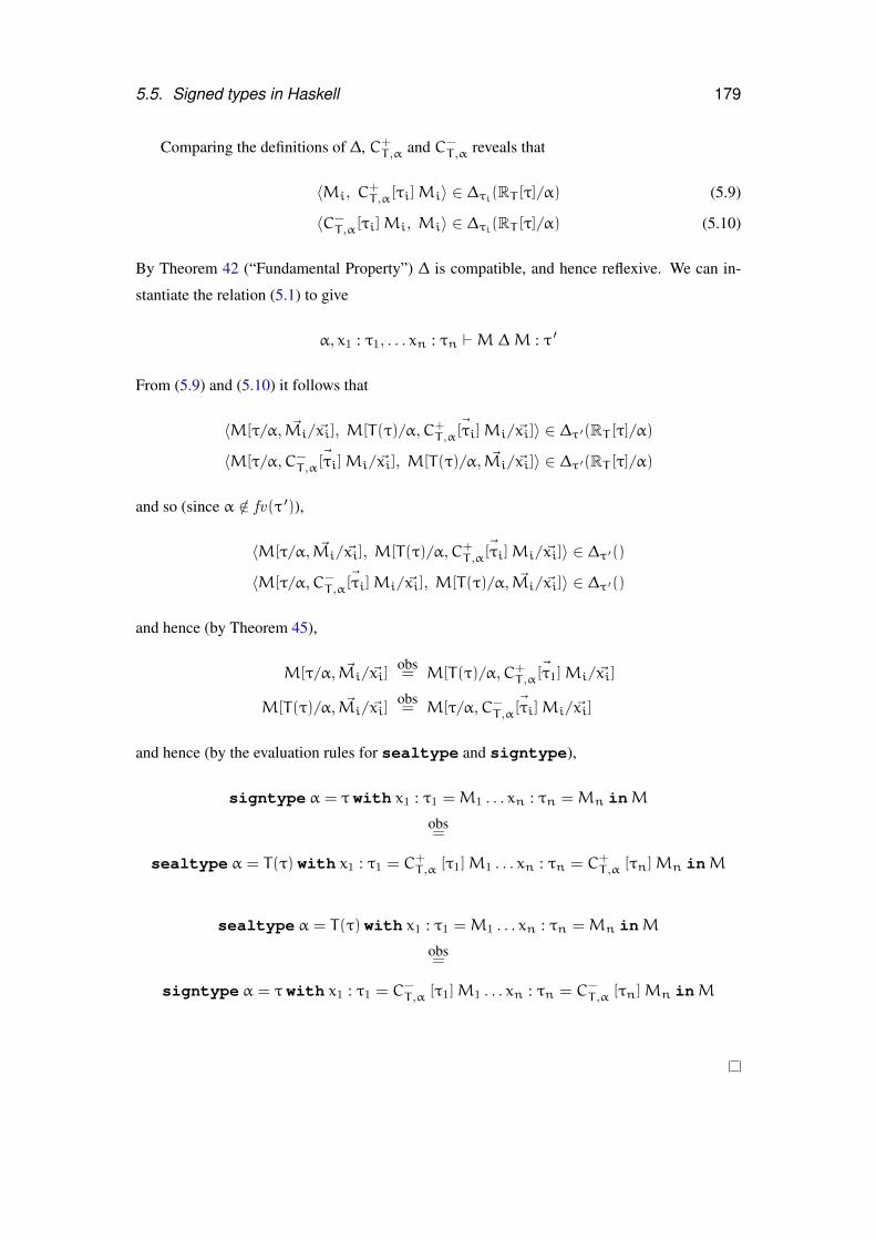
5.5. Signed types in Haskell 179
Comparing the definitions of ∆, C+T ,α and C−
T ,α reveals that
〈Mi, C+T ,α[τi]Mi〉 ∈ ∆τi(RT [τ]/α) (5.9)
〈C−T ,α[τi]Mi, Mi〉 ∈ ∆τi(RT [τ]/α) (5.10)
By Theorem 42 (“Fundamental Property”) ∆ is compatible, and hence reflexive. We can in-
stantiate the relation (5.1) to give
α, x1 : τ1, . . . xn : τn `M ∆M : τ ′
From (5.9) and (5.10) it follows that
〈M[τ/α, ~Mi/~xi], M[T(τ)/α, ~C+T ,α[τi]Mi/~xi]〉 ∈ ∆τ ′(RT [τ]/α)
〈M[τ/α, ~C−T ,α[τi]Mi/~xi], M[T(τ)/α, ~Mi/~xi]〉 ∈ ∆τ ′(RT [τ]/α)
and so (since α /∈ fv(τ ′)),
〈M[τ/α, ~Mi/~xi], M[T(τ)/α, ~C+T ,α[τi]Mi/~xi]〉 ∈ ∆τ ′()
〈M[τ/α, ~C−T ,α[τi]Mi/~xi], M[T(τ)/α, ~Mi/~xi]〉 ∈ ∆τ ′()
and hence (by Theorem 45),
M[τ/α, ~Mi/~xi]obs= M[T(τ)/α, ~C+
T ,α[τ1]Mi/~xi]
M[T(τ)/α, ~Mi/~xi]obs= M[τ/α, ~C−
T ,α[τi]Mi/~xi]
and hence (by the evaluation rules for sealtype and signtype),
signtype α = τ with x1 : τ1 =M1 . . . xn : τn =Mn inM
obs=
sealtype α = T(τ) with x1 : τ1 = C+T ,α [τ1]M1 . . . xn : τn = C+
T ,α [τn]Mn inM
sealtype α = T(τ) with x1 : τ1 =M1 . . . xn : τn =Mn inM
obs=
signtype α = τ with x1 : τ1 = C−T ,α [τ1]M1 . . . xn : τn = C−
T ,α [τn]Mn inM
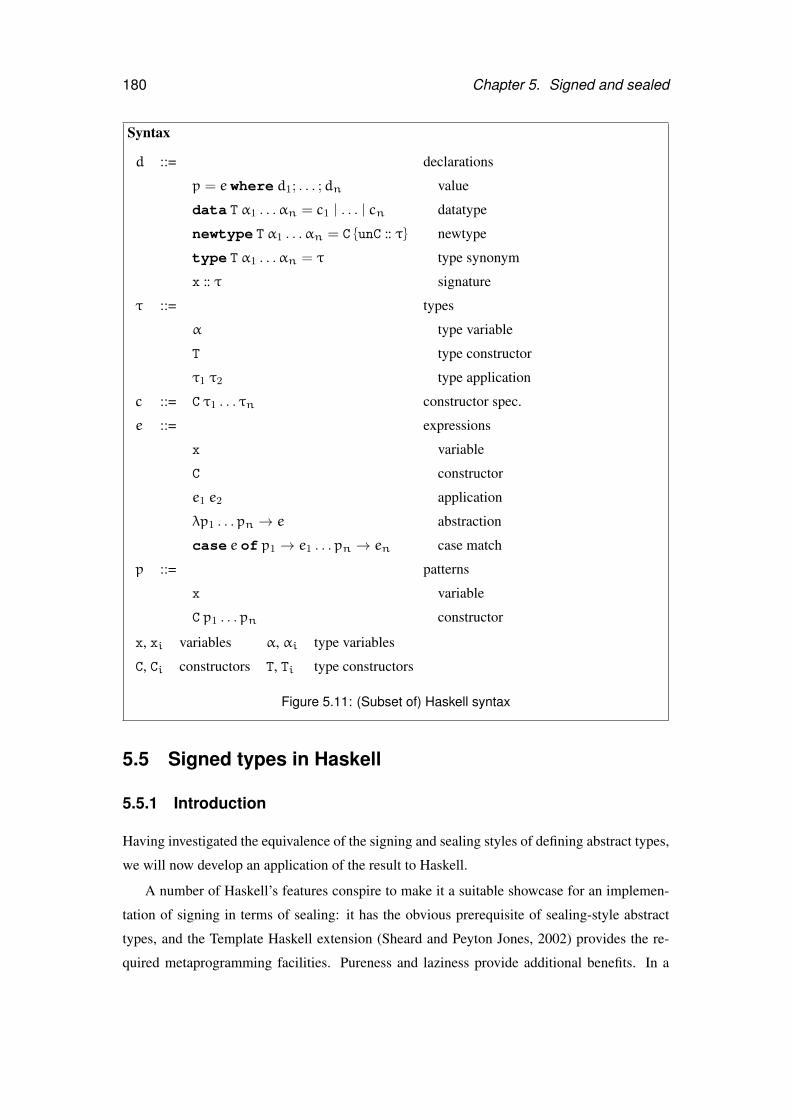
180 Chapter 5. Signed and sealed
Syntax
d ::= declarations
p = e where d1; . . . ;dn value
data T α1 . . .αn = c1 | . . . | cn datatype
newtype T α1 . . .αn = C {unC :: τ} newtype
type T α1 . . .αn = τ type synonym
x :: τ signature
τ ::= types
α type variable
T type constructor
τ1 τ2 type application
c ::= C τ1 . . . τn constructor spec.
e ::= expressions
x variable
C constructor
e1 e2 application
λp1 . . .pn → e abstraction
case e of p1 → e1 . . .pn → en case match
p ::= patterns
x variable
C p1 . . .pn constructor
x, xi variables α, αi type variables
C, Ci constructors T, Ti type constructors
Figure 5.11: (Subset of) Haskell syntax
5.5 Signed types in Haskell
5.5.1 Introduction
Having investigated the equivalence of the signing and sealing styles of defining abstract types,
we will now develop an application of the result to Haskell.
A number of Haskell’s features conspire to make it a suitable showcase for an implemen-
tation of signing in terms of sealing: it has the obvious prerequisite of sealing-style abstract
types, and the Template Haskell extension (Sheard and Peyton Jones, 2002) provides the re-
quired metaprogramming facilities. Pureness and laziness provide additional benefits. In a
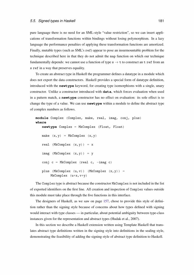
5.5. Signed types in Haskell 181
pure language there is no need for an SML-style “value restriction”, so we can insert appli-
cations of transformation functions within bindings without losing polymorphism. In a lazy
language the performance penalties of applying these transformation functions are amortized.
Finally, mutable types (such as SML’s ref) appear to pose an insurmountable problem for the
technique described here in that they do not admit the map function on which our technique
fundamentally depends: we cannot use a function of type s→ t to construct an t ref from an
s ref in a way that preserves equality.
To create an abstract type in Haskell the programmer defines a datatype in a module which
does not export the data constructors. Haskell provides a special form of datatype definition,
introduced with the newtype keyword, for creating type isomorphisms with a single, unary
constructor. Unlike a constructor introduced with data, which forces evaluation when used
in a pattern match, a newtype constructor has no effect on evaluation: its sole effect is to
change the type of a value. We can use newtype within a module to define the abstract type
of complex numbers as follows.
module Complex (Complex, make, real, imag, conj, plus)where
newtype Complex = MkComplex (Float, Float)
make (x,y) = MkComplex (x,y)
real (MkComplex (x,y)) = x
imag (MkComplex (x,y)) = y
conj c = MkComplex (real c, -imag c)
plus (MkComplex (u,v)) (MkComplex (x,y)) =MkComplex (u+x,v+y)
The Complex type is abstract because the constructor MkComplex is not included in the list
of exported identifiers on the first line. All creation and inspection of Complex values outside
this module must take place through the five functions in this interface.
The designers of Haskell, as we saw on page 157, chose to provide this style of defini-
tion rather than the signing style because of concerns about how types defined with signing
would interact with type classes — in particular, about potential ambiguity between type-class
instances given for the representation and abstract types (Hudak et al., 2007).
In this section we describe a Haskell extension written using Template Haskell that trans-
lates abstract type definitions written in the signing style into definitions in the sealing style,
demonstrating the feasibility of adding the signing style of abstract type definition to Haskell.
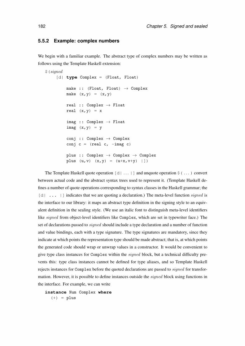
182 Chapter 5. Signed and sealed
5.5.2 Example: complex numbers
We begin with a familiar example. The abstract type of complex numbers may be written as
follows using the Template Haskell extension:
$(signed[d| type Complex = (Float, Float)
make :: (Float, Float) → Complex
make (x,y) = (x,y)
real :: Complex → Float
real (x,y) = x
imag :: Complex → Float
imag (x,y) = y
conj :: Complex → Complex
conj c = (real c, -imag c)
plus :: Complex → Complex → Complex
plus (u,v) (x,y) = (u+x,v+y) |])
The Template Haskell quote operation [d| . . . |] and unquote operation $( . . . ) convert
between actual code and the abstract syntax trees used to represent it. (Template Haskell de-
fines a number of quote operations corresponding to syntax classes in the Haskell grammar; the
[d| ... |] indicates that we are quoting a declaration.) The meta-level function signed is
the interface to our library: it maps an abstract type definition in the signing style to an equiv-
alent definition in the sealing style. (We use an italic font to distinguish meta-level identifiers
like signed from object-level identifiers like Complex, which are set in typewriter face.) The
set of declarations passed to signed should include a type declaration and a number of function
and value bindings, each with a type signature. The type signatures are mandatory, since they
indicate at which points the representation type should be made abstract; that is, at which points
the generated code should wrap or unwrap values in a constructor. It would be convenient to
give type class instances for Complex within the signed block, but a technical difficulty pre-
vents this: type class instances cannot be defined for type aliases, and so Template Haskell
rejects instances for Complex before the quoted declarations are passed to signed for transfor-
mation. However, it is possible to define instances outside the signed block using functions in
the interface. For example, we can write
instance Num Complex where(+) = plus
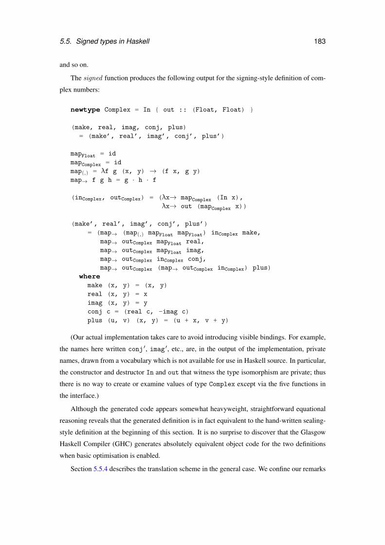
5.5. Signed types in Haskell 183
and so on.
The signed function produces the following output for the signing-style definition of com-
plex numbers:
newtype Complex = In { out :: (Float, Float) }
(make, real, imag, conj, plus)= (make’, real’, imag’, conj’, plus’)
mapFloat = id
mapComplex = id
map(,) = λf g (x, y) → (f x, g y)map→ f g h = g · h · f
(inComplex, outComplex) = (λx→ mapComplex (In x),λx→ out (mapComplex x))
(make’, real’, imag’, conj’, plus’)= (map→ (map(,) mapFloat mapFloat) inComplex make,
map→ outComplex mapFloat real,map→ outComplex mapFloat imag,map→ outComplex inComplex conj,map→ outComplex (map→ outComplex inComplex) plus)
wheremake (x, y) = (x, y)real (x, y) = x
imag (x, y) = y
conj c = (real c, -imag c)plus (u, v) (x, y) = (u + x, v + y)
(Our actual implementation takes care to avoid introducing visible bindings. For example,
the names here written conj ′, imag ′, etc., are, in the output of the implementation, private
names, drawn from a vocabulary which is not available for use in Haskell source. In particular,
the constructor and destructor In and out that witness the type isomorphism are private; thus
there is no way to create or examine values of type Complex except via the five functions in
the interface.)
Although the generated code appears somewhat heavyweight, straightforward equational
reasoning reveals that the generated definition is in fact equivalent to the hand-written sealing-
style definition at the beginning of this section. It is no surprise to discover that the Glasgow
Haskell Compiler (GHC) generates absolutely equivalent object code for the two definitions
when basic optimisation is enabled.
Section 5.5.4 describes the translation scheme in the general case. We confine our remarks
184 Chapter 5. Signed and sealed
here to a couple of key points.
The most obvious distinction between the code generated by the Template Haskell exten-
sion and the PolyPCF code generated by the translation between tagged and untagged repre-
sentations of abstract types (Section 5.3.2) is the large number of calls to mapT functions in the
former, which do not appear at all in the latter. The explanation is simple: Haskell allows the
definition of new type constructors using the type, data and newtype constructs, whereas
type constructors in PolyPCF are limited to a predefined set, namely list, →, T(−) and ∀.Each mapT function is used to traverse structures of type T τ1 . . . τn in order to add tags to
any values of type Complex located within. In the PolyPCF translation of Section 5.3.2 these
traversals are simply written out inline for each type constructor.
The type alias (defined with type) used in the input declaration is replaced in the out-
put with a newtype definition. The inComplex and outComplex functions are used to add and
remove the constructor for the Complex type at places where the type signatures in the input
definition indicate that the type should be abstract. They serve two functions: inComplex both
adds a constructor to a Complex value and traverses the value in order to add constructors to
any Complex values found within. (In this case the traversal is trivial, since there can never
be a Complex within a Complex; for parameterised abstract types the traversal is non-trivial,
as shown in Section 5.5.4.3.) The primed variables are used to distinguish the transformed
functions such as real’ which act upon the abstract type (Complex) from the original func-
tions such as real which act upon its representation ((Float, Float)). Thus, the reference to
real within the definition of conj refers to the original, not the transformed, version of the
function. (In Haskell, unlike in PolyPCF, bindings may generally be mutually recursive. We
take advantage of this facility here, using the real and imag functions to implement conj.)
5.5.3 Example: a sudoku solver
The Complex example illustrates the connection between our Template Haskell library and the
ML and PolyPCF programs in Sections 5.1–5.4. We now give a further example that highlights
some distinctive properties of the Template Haskell implementation and shows its applicability
to an existing program.
Bird (2006) presents a Haskell program for solving Sudoku puzzles. The development
begin by defining types to represent boards. A Sudoku board is a square matrix of characters,
which is represented as a list of lists:
type Matrix α = [[α]]type Board = Matrix Char
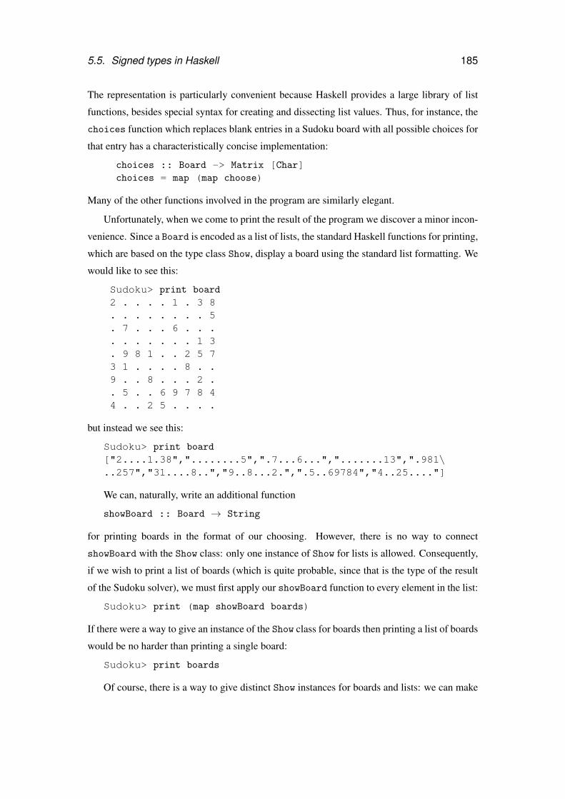
5.5. Signed types in Haskell 185
The representation is particularly convenient because Haskell provides a large library of list
functions, besides special syntax for creating and dissecting list values. Thus, for instance, the
choices function which replaces blank entries in a Sudoku board with all possible choices for
that entry has a characteristically concise implementation:
choices :: Board -> Matrix [Char]choices = map (map choose)
Many of the other functions involved in the program are similarly elegant.
Unfortunately, when we come to print the result of the program we discover a minor incon-
venience. Since a Board is encoded as a list of lists, the standard Haskell functions for printing,
which are based on the type class Show, display a board using the standard list formatting. We
would like to see this:
Sudoku> print board
2 . . . . 1 . 3 8. . . . . . . . 5. 7 . . . 6 . . .. . . . . . . 1 3. 9 8 1 . . 2 5 73 1 . . . . 8 . .9 . . 8 . . . 2 .. 5 . . 6 9 7 8 44 . . 2 5 . . . .
but instead we see this:
Sudoku> print board
["2....1.38","........5",".7...6...",".......13",".981\..257","31....8..","9..8...2.",".5..69784","4..25...."]
We can, naturally, write an additional function
showBoard :: Board → String
for printing boards in the format of our choosing. However, there is no way to connect
showBoard with the Show class: only one instance of Show for lists is allowed. Consequently,
if we wish to print a list of boards (which is quite probable, since that is the type of the result
of the Sudoku solver), we must first apply our showBoard function to every element in the list:
Sudoku> print (map showBoard boards)
If there were a way to give an instance of the Show class for boards then printing a list of boards
would be no harder than printing a single board:
Sudoku> print boards
Of course, there is a way to give distinct Show instances for boards and lists: we can make
186 Chapter 5. Signed and sealed
Board a distinct type (using newtype) rather than an alias (using type). Unfortunately,
while this solves the printing problem, it makes the implementation of the solver much less
elegant. Suppose that the type of boards is defined as follows:
newtype Board = MkBoard { unBoard :: Matrix Char}
We must now add code to many of the functions that implement the Sudoku solver to add and
remove the MkBoard constructor, resulting in an undesirable increase in the size of the code.
For example, the choices function becomes
choices :: Board -> Matrix [Char]choices = map (map choose) · unBoard
The idea of the extension described in this section is to allow us the advantages of both ap-
proaches: we can define boards directly in terms of lists, enabling an elegant implementation
of the solver, while making the type Board distinct from the list type, allowing us to customise
the behaviour of overloaded functions such as show. A further benefit of moving from a type
alias to an abstract type is the potential to enforce constraints, such as board squareness, that
are not captured by the representation type.
5.5.4 The translation
We now turn to the specification of the translation.
Translation of the definition of an abstract type constructor T from the signing style to the
sealing style involves four meta-level functions, which we describe in Sections 5.5.4.1–5.5.4.4.
The first function, tynames , (Section 5.5.4.1) determines the set of type constructors involved
in the representation type and operations of T. The second function, map, (Section 5.5.4.2)
uses the definition of each type constructor to generate a corresponding map function. The
third function, tag , (Section 5.5.4.3) creates functions that convert between values of the ab-
stract type T and values of the corresponding representation type. The final function, tr , (Sec-
tion 5.5.4.4) generates functions that convert each operation in the abstract type definition from
the signing style to the sealing style. The meta-level function signed (Section 5.5.4.5) which
translates from signing-style to a sealing-style definition, is defined in terms of these four func-
tions.
5.5.4.1 Finding type constructors (tynames)
Both the representation of an abstract type and the signatures of the operations on the type are
given in terms of type constructors which are defined elsewhere in the program or provided
as standard. For example, the representation of the Complex type is built from the type con-
5.5. Signed types in Haskell 187
structor for pairs, written (, ), and the nullary type constructor Float. The operations on the
Complex type also use the function type constructor,→. Inserting and removing tags involves
traversing values whose shape is specified by the definitions of these type constructors; in order
to traverse these values we must therefore generate a mapT function for each type constructor
T. The definition of mapT depends on the definition of T, to which we therefore require ac-
cess; retrieving the definition of a type constructor (or other identifier) is the purpose of the
reify function supplied with Template Haskell. Building on reify , we can retrieve the set of
all type constructors used in a type expression, whether they appear in the expression itself or
in the definition of some other type constructor which is used by the expression. We begin
by giving three Template Haskell functions — tynamesD, tynamesC and tynamesE — that
compute the set of type constructors used, respectively, in a type definition, a data constructor
specification, and a type expression.
The tynamesD function takes two arguments: a type declaration, written between brackets,
and a set r of the type constructors already seen. For data and newtype declarations we must
collect both the type constructor T on the left hand side and any type constructors used in the
constructor specifications. We add T to r when examining constructor specifications, since
these may use T if the type is recursive.
tynamesD [data T α1 . . .αn = c1 | . . . | cn] r
= {T} ∪ tynamesC [c1] (r ∪ {T}) ∪ . . . ∪ tynamesC [cn] (r ∪ {T})
tynamesD [newtype T α1 . . .αn = C {x :: τ}] r
= {T } ∪ tynamesE [τ] (r ∪ {T})
A type declaration cannot be recursive, so we pass through r unchanged. The result
consists of the type constructor on the left hand side of the declaration and any type constructors
used on the right hand side.
tynamesD [type T α1 . . .αn = τ] r = {T } ∪ tynamesE [τ] r
Finding the type constructors used in a constructor specification is simply a matter of ex-
amining the type expressions which specify the domain of the constructor.
tynamesC [C τ1 . . . τn] r = tynamesE [τ1] r . . . tynamesE [τn] r
The tynamesE function finds the type constructors used, directly or indirectly, in a type
expression. A type expression consisting of a type variable does not use any type constructors:
tynamesE [α] r = {}
For a type expression consisting of a type constructor T the result depends on whether T is
found in r. If it is then we are in the process of examining the definition of T already, so there
188 Chapter 5. Signed and sealed
is nothing more to do. If not, then the set of type constructors used consists of both T and all
of the type constructors used in the definition of T , which we retrieve using reify .
tynamesE [T] r = {} if T ∈ r{T} ∪ tynamesD [reify T] r otherwise
For a type application we simply examine the sub-expressions to determine the set of type
constructors involved.
tynamesE [τ1 τ2] r = tynamesE τ1 r ∪ tynamesE τ2 r
5.5.4.2 Generating map functions (map)
The next step is to generate functions mapT for each type constructor T used in the definition of
the abstract type. These perform the bulk of the work in translating from the signing style to
the sealing style. The type of each mapT function depends the way that the type parameters to
T are used in its definition. A type constructor T with n parameters, all of which are used both
positively and negatively within the definition of T, results in a function mapT of the type
(α1→β1,β1→α1)→. . .→ (αn→βn,βn→αn)→ Tα1 . . .αn→ Tβ1 . . .βn
— that is, with a pair of functions for each parameter of T, to transform positive and negative
occurrences of the parameter. If a type parameter is only used positively then the second com-
ponent of the pair is omitted in the corresponding parameter to the generated mapT function.
For type parameters that are only used negatively, the first component is omitted. For “phan-
tom” type parameters, not used at all in the definition of T, there is no corresponding function
parameter.
There are four type constructors involved in the definition of Complex: Float, Complex,
(, ) and→. The first two of these, Float and Complex, are nullary, and so the associated map
functions are equivalent to the identity function. The map function for the pair type, map(,),
has type:
(α→ γ)→ (β→ δ)→ (α,β)→ (γ, δ)
In this case the parameters to map(,) are functions for transforming positive occurrences of the
corresponding type variables, since the type parameters to the pair type only occur positively in
its definition. We must distinguish between positive and negative occurrences, since at positive
occurrences of the type constructor Complex we will insert calls to In to convert from the
representation to the abstract type, and at negative occurrences we will insert calls to out. The
map→ function has two function parameters, reflecting the two type parameters to the function
type constructor →, the first (denoting the argument type on the function) negative and the
5.5. Signed types in Haskell 189
second (denoting the return type) positive. Consequently, the generated map function has the
following type:
(γ→ α)→ (β→ δ)→ (α→ β)→ (γ→ δ)
We use an auxiliary function, param , to construct parameters for generated functions, writing
param(αi, T) = (pi, ni)
if αi occurs positively and negatively within T’s definition
param(αi, T) = pi
if αi occurs only positively within T’s definition
param(αi, T) = ni
if αi occurs only negatively within T’s definition
param(αi, T) = (i.e. nothing)
if αi does not occur within T’s definition
Each parameter pi of the generated function corresponds to a function which transforms the
positive occurrences of the ith type parameter, αi; each ni acts similarly on negative occur-
rences. If there are no positive occurrences of αi then pi is omitted; similarly, ni is omitted if
αi does not occur negatively.
We now turn to the definitions of the Template Haskell functions which generate the map
functions. Once again we give three Template Haskell functions, treating type definitions, type
expressions, and data constructor specifications. The mapD function generates a map function
for a type definition. There are three cases, one for each type-constructor-introducing keyword.
For a data declaration we generate a case match over the constructors of the declared
datatype, delegating generation of the matches to the mapC function. The substitution [αi 7→(pi, ni)] passed to mapC records the correspondence between type variables and parameters.
mapD[data T α1 . . .αn = c1 | . . . | cn]
= λ param(α1, T) . . . param(αn, T) x→case x of
mapC[c1][αi 7→ (pi, ni)]
. . .
mapC[cn][αi 7→ (pi, ni)]
The treatment of newtype is similar, save that there is only one constructor to consider.
mapD[newtype T α1 . . .αn = C {unC :: τ}]
= λ param(α1, T) . . . param(αn, T) x→case x of
mapC[C τ][αi 7→ (pi, ni)]
190 Chapter 5. Signed and sealed
For alias declarations, declared with type, the mapE function does all of the work.
mapD[type T α1 . . .αn = τ]
= λ param(α1, T) . . . param(αn, T) x→map+E [τn][αi 7→ (pi, ni)] x
The mapC function treats constructor specifications, generating a case match for a data
constructor. The xi variables bind the constructor parameters, and we use mapE to transform
each parameter, finally applying the constructor C.
mapC [C τ1 . . . τn] r = C x1 . . . xn → C (map+E [τ1] r x1) . . . (map+E [τn] r xn)
The mapE function generates, for a type τ with free variables α1 . . .αn, a term t with
free variables p1 . . . pn, n1 . . . nn. If each of the pi has type αi → βi and each of the ni has
type βi → αi then t will have type τ → τ[ ~βi/ ~αi]. Besides the substitution parameter r and
the parameter between brackets which denotes a type expression there is a further parameter
to mapC representing the “polarity” of the expression, i.e. whether type variables occurring
in the expression represent input or output parameters. At a type variable αi we project out
the first or second component of the corresponding pair of functions (pi, ni), depending on the
polarity.
map+E [αi] r = pi where r(αi) = (pi, ni)
map−E [αi] r = ni where r(αi) = (pi, ni)
At a type constructor T we generate a (possibly recursive) call to the map function for T.
mappE [T ] r = mapT
At type applications τ1 τ2 we generate function applications. The function component is gen-
erated from τ1 by mapE. The argument that is generated depends on the type of the generated
function expression (which, in turn, depends on the variance of the type constructor that is
involved). We write p̄ to reverse the polarity of p. Then we generate the following application
expressions from type applications:
mappE [τ1 τ2] r = mappE [τ1] r (mappE [τ2] r,mapp̄E [τ2] r)
if τ2 is the argument for a type parameter that is used both positively and negatively.
mappE [τ1 τ2] r = mappE [τ1] r (mappE [τ2] r)
if τ2 is the argument for a type parameter that is used only positively.
mappE [τ1 τ2] r = mappE [τ1] r (mapp̄E [τ2] r)
if τ2 is the argument for a type parameter that is used only negatively.
mappE [τ1 τ2] r = mappE [τ1] r
if τ2 is the argument for a phantom type parameter.
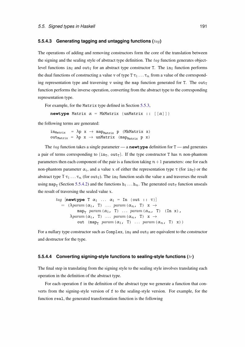
5.5. Signed types in Haskell 191
5.5.4.3 Generating tagging and untagging functions (tag)
The operations of adding and removing constructors form the core of the translation between
the signing and the sealing style of abstract type definition. The tag function generates object-
level functions inT and outT for an abstract type constructor T. The inT function performs
the dual functions of constructing a value v of type T τ1 . . . τn from a value of the correspond-
ing representation type and traversing v using the map function generated for T. The outT
function performs the inverse operation, converting from the abstract type to the corresponding
representation type.
For example, for the Matrix type defined in Section 5.5.3,
newtype Matrix α = MkMatrix {unMatrix :: [[α]]}
the following terms are generated:
inMatrix = λp x → mapMatrix p (MkMatrix x)outMatrix = λp x → unMatrix (mapMatrix p x)
The tag function takes a single parameter — a newtype definition for T — and generates
a pair of terms corresponding to (inT, outT). If the type constructor T has n non-phantom
parameters then each component of the pair is a function taking n+1 parameters: one for each
non-phantom parameter αi, and a value x of either the representation type τ (for inT) or the
abstract type T τ1 . . . τn (for outT). The inT function seals the value x and traverses the result
using mapT (Section 5.5.4.2) and the functions h1 . . . hn. The generated outT function unseals
the result of traversing the sealed value x.
tag [newtype T α1 . . . α1 = In {out :: τ}]= (λparam(α1, T) . . . param(αn, T) x →
mapT param(α1, T) . . . param(αn, T) (In x),λparam(α1, T) . . . param(αn, T) x →
out (mapT param(α1, T) . . . param(αn, T) x))
For a nullary type constructor such as Complex, inT and outT are equivalent to the constructor
and destructor for the type.
5.5.4.4 Converting signing-style functions to sealing-style functions (tr )
The final step in translating from the signing style to the sealing style involves translating each
operation in the definition of the abstract type.
For each operation f in the definition of the abstract type we generate a function that con-
verts from the signing-style version of f to the sealing-style version. For example, for the
function real, the generated transformation function is the following
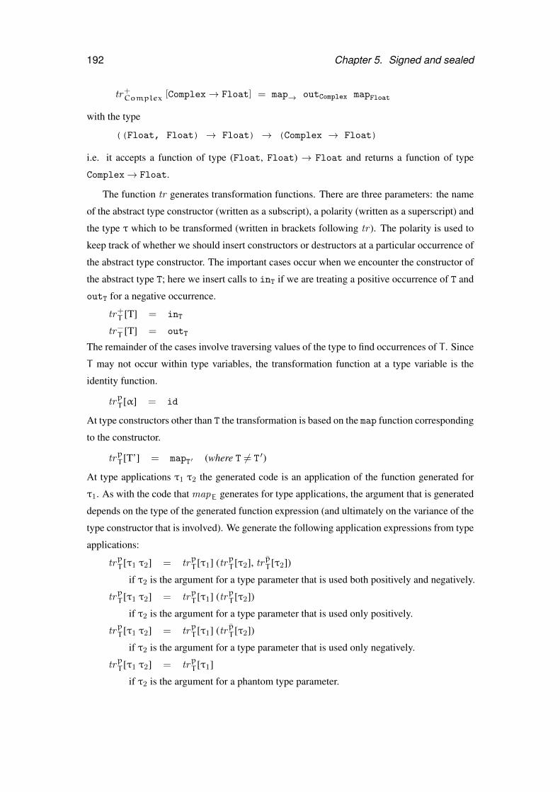
192 Chapter 5. Signed and sealed
tr+Complex [Complex→ Float] = map→ outComplex mapFloat
with the type
((Float, Float) → Float) → (Complex → Float)
i.e. it accepts a function of type (Float, Float) → Float and returns a function of type
Complex→ Float.
The function tr generates transformation functions. There are three parameters: the name
of the abstract type constructor (written as a subscript), a polarity (written as a superscript) and
the type τ which to be transformed (written in brackets following tr ). The polarity is used to
keep track of whether we should insert constructors or destructors at a particular occurrence of
the abstract type constructor. The important cases occur when we encounter the constructor of
the abstract type T; here we insert calls to inT if we are treating a positive occurrence of T and
outT for a negative occurrence.
tr+T [T] = inT
tr−T [T] = outT
The remainder of the cases involve traversing values of the type to find occurrences of T . Since
T may not occur within type variables, the transformation function at a type variable is the
identity function.
trpT [α] = id
At type constructors other than T the transformation is based on the map function corresponding
to the constructor.
trpT [T’] = mapT ′ (where T 6= T ′)
At type applications τ1 τ2 the generated code is an application of the function generated for
τ1. As with the code that mapE generates for type applications, the argument that is generated
depends on the type of the generated function expression (and ultimately on the variance of the
type constructor that is involved). We generate the following application expressions from type
applications:
trpT [τ1 τ2] = trpT [τ1] (trpT [τ2], tr p̄T [τ2])
if τ2 is the argument for a type parameter that is used both positively and negatively.
trpT [τ1 τ2] = trpT [τ1] (trpT [τ2])
if τ2 is the argument for a type parameter that is used only positively.
trpT [τ1 τ2] = trpT [τ1] (tr p̄T [τ2])
if τ2 is the argument for a type parameter that is used only negatively.
trpT [τ1 τ2] = trpT [τ1]
if τ2 is the argument for a phantom type parameter.
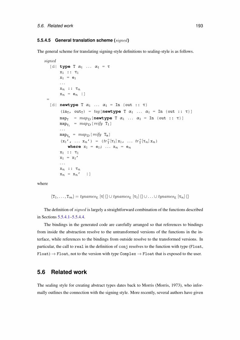
5.6. Related work 193
5.5.4.5 General translation scheme (signed )
The general scheme for translating signing-style definitions to sealing-style is as follows.
signed[d| type T α1 . . . α1 = τ
x1 :: τ1
x1 = e1
. . .xn :: τnxn = en |]
=[d| newtype T α1 . . . α1 = In {out :: τ}
(inT, outT) = tag[newtype T α1 . . . α1 = In {out :: τ}]
mapT = mapD[newtype T α1 . . . α1 = In {out :: τ}]mapT1 = mapD[reify T1]. . .mapTm = mapD[reify Tm]
(x1’, . . . xn’) = (tr+T [τ1] x1, . . . tr+T [τn] xn)where x1 = e1; . . . xn = en
x1 :: τ1
x1 = x1’. . .xn :: τnxn = xn’ |]
where
{T1, . . . , Tm} = tynamesE [τ] {} ∪ tynamesE [τ1] {} ∪ . . . ∪ tynamesE [τn] {}
The definition of signed is largely a straightforward combination of the functions described
in Sections 5.5.4.1–5.5.4.4.
The bindings in the generated code are carefully arranged so that references to bindings
from inside the abstraction resolve to the untransformed versions of the functions in the in-
terface, while references to the bindings from outside resolve to the transformed versions. In
particular, the call to real in the definition of conj resolves to the function with type (Float,
Float)→ Float, not to the version with type Complex→ Float that is exposed to the user.
5.6 Related work
The sealing style for creating abstract types dates back to Morris (Morris, 1973), who infor-
mally outlines the connection with the signing style. More recently, several authors have given
194 Chapter 5. Signed and sealed
formal translations between static and dynamic schemes for preserving types. It is not surpris-
ing that the translations are similar in each case, although their motivations (and consequently
the precise properties that they investigate) differ considerably.
Sumii and Pierce (Sumii and Pierce, 2004) have examined the relationship between type
abstraction and cryptography, developing a theory of relational parametricity for their crypto-
graphic λ-calculus. They give an encoding of type abstraction into encryption (but not vice
versa); their encryption primitives, which give a variant of dynamic sealing, are significantly
more expressive than our tags, so the inverse translation is not straightforward.
Matthews and Findler (Matthews and Findler, 2009) investigate the semantics of programs
written in multiple languages — partly in Scheme and partly in ML. They investigate two ways
to encode foreign values: as opaque “lumps” that must be explicitly passed to the language
which created them each time they are used, or as values that have been wrapped using a type-
directed strategy, so that they can be used directly. The wrappings, which dynamically check
that the values they wrap have the appropriate shapes, are an instance of higher-order contracts
(Findler and Felleisen, 2002); the type-directed scheme for inserting guards is analogous to our
translation from signing-style to sealing-style abstract types.
Matthews and Ahmed (Matthews and Ahmed, 2008) extend Matthews and Findler’s system
with polymorphism, and prove a parametricity property. In order to such prevent violations
of parametricity as can arise from dynamic inspection of values by the Scheme portion of a
program, they dynamically seal values of abstract type before passing them to Scheme.
5.7 Future work
Abstract types The central result of Sections 5.1–5.4 establishes an equivalence between
translations of the two styles of abstract type within the context of a single program (namely
the continuationM of the signtype and sealtype constructs). More traditionally, abstract
types are represented using existential types; we might obtain a stronger result by translating
signtype to an existential type and sealtype to some other appropriate type (perhaps
extending PolyPCF with scoped data constructors, rather than globally-available tags), then
showing that the two are isomorphic up to observational equivalence.
We have, in this chapter, investigated a comparatively simple notion of abstract type. Mod-
ern ML-family languages (Milner, Tofte, Harper, and MacQueen, 1997, Romanenko, Russo,
and Sestoft, 2000, Leroy, 2008) typically support considerably more elaborate mechanisms for
creating abstract types: nested signatures, parameterised modules (functors), recursive mod-
ules, and so on. Further, in our work the number of seals is statically fixed for each program.
5.7. Future work 195
This concords with the features provided by Haskell and SML, but is less general than mecha-
nisms used in Scheme, where seals may be created dynamically. The question naturally arises
whether the scheme given here can be extended to treat these more general systems.
Overloading We have shown that the two styles of type abstraction commonly found in
functional programming languages are equivalent and inter-definable. The language designer
is therefore free to provide either style, without danger of loss of expressiveness. There is a
similar dichotomy in the design space of overloaded functions: should we base method res-
olution on the types of the program, or on its values? The designers of Haskell have chosen
the first option: values are typically represented uniformly, and method resolution in Haskell
can be influenced by type annotations. Object-oriented languages typically take the second
route, inspecting values at runtime to select a suitable method implementation. To what extent
are these approaches compatible? Can we design a system which admits either compilation
strategy? Odersky, Wadler, and Wehr (1995) resolve some of these questions, by requiring that
the type variable denoting the instance type appear as the first argument of every overloaded
method. It remains to be seen whether a system such as Odersky et al.’s (1995) can incorporate
features of the modern system of Haskell type classes, such as constructor classes and associ-
ated types (Chakravarty, Keller, and Peyton Jones, 2005a, Chakravarty, Keller, Peyton Jones,
and Marlow, 2005b).

Chapter 6
Conclusion
6.1 Contributions
Our study of three interfaces to computation — idioms, arrows, and monads — revealed that
idioms are the weakest of the three, an adjustment to the informal claims of McBride and
Paterson (2008). We have proved that the arrow calculus, a variant of Paterson’s notation, is in
equational correspondence with the classical presentation of arrows. Using the arrow calculus,
we have shown that idioms correspond to those arrows which are isomorphic to oblivious
computations that return functions:
A B ∼= 1 (A→ B)
and that monads correspond to those arrows which are isomorphic to functions that construct
computations:
A B ∼= A→ (1 B)
Additionally, we have used the laws of each interface to construct normalising transformers for
idioms, arrows and monads in Haskell.
We used our results about idioms, arrows and monads to guide the design of a library, form-
lets, for compositional construction of HTML forms. The semantics of formlets are given in
terms of three primitive idioms, which capture the effects involved in form construction: fresh
name generation, XML construction, and reading values from an environment. While each of
these idioms is also a monad, their composition as the formlet idiom is not a monad; in fact, we
argue that idioms, the weakest of the three interfaces, are the most suitable basis for formlets.
Our description of the formlet library is intended to reveal the “essence” of form abstraction,
and the result is accordingly simple. Nevertheless, formlets extend readily to more realistic
settings. We have shown how to support validation of user input by incorporating an idiom
197
198 Chapter 6. Conclusion
that captures failure, and how to give static guarantees of XHTML validity by using indexed
idioms, an analogue of indexed monads (Wadler and Thiemann, 2003, Abadi, 2007). Formlets
also come equipped with a convenient syntax; we have given a desugaring of this syntax into
applications of the idiom operations and an alternative, more efficient, desugaring based on
multi-holed contexts and parameterised idioms (an analogue of Atkey’s (2009) parameterised
monads).
The formlets library depends on continuations that persist between requests. Links uses a
stateless-server approach, embedding serialised continuations within the page sent to the client,
to be sent back to the server with subsequent requests. Code for serialisation typically recapit-
ulates the structure of the type to be serialised; we avoid this in the Links implementation by
using an analogue of Haskell’s deriving mechanism for automatically constructing overloaded
function instances from type declarations. The design of our deriving for OCaml (the Links
implementation language) is guided by the well-known correspondence between type classes
and ML-style modules. We have described the implementation of a structure-sharing serialiser,
Pickle, in the deriving framework, and shown how giving custom instances for equality and
hashing (superclasses of Pickle) can improve the compactness of its output without the need
to change any serialisation code. We illustrated this using a serialiser for lambda terms that
is customised to consider alpha-equivalent terms equal, resulting in more compact output than
serialisers which treat terms as simple trees.
Our final chapter investigated the two common styles of abstract type definition, in which
the abstraction boundary is drawn either in the terms, using a private data constructor (“seal-
ing”), or in the types, using a signature (“signing”). We extended Pitts’s (2000) partial poly-
morphic lambda calculus, PolyPCF, with constructs for both styles and used parametricity to
show that they are inter-definable. To demonstrate the utility of the equivalence we gave a
implementation of the signing style in Template Haskell, showing how programs written in the
signing style can be translated into the sealing style, addressing concerns about ambiguity that
led the Haskell designers to choose the latter over the former.
6.2 The status of Links
The ideas described in this dissertation were developed in the context of the Links project. The
reader may therefore be interested in a brief summary of the current status of Links.
There is a small community of Links users, with a mailing list of around seventy mem-
bers. Work on the implementation continues, with further releases planned for the near future.
Researchers in Maryland and Cambridge have developed variants of Links with integrated

6.2. The status of Links 199
support for security (Swamy, Hicks, and Tsang, 2007, Corcoran, Swamy, and Hicks, 2007,
Swamy, Corcoran, and Hicks, 2008, Corcoran, Swamy, and Hicks, 2009, Baltopoulos and Gor-
don, 2009). Finally, researchers in Edinburgh are applying for funding to continue development
of Links.

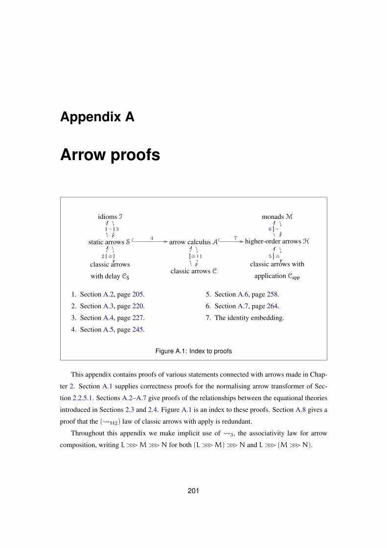
Appendix A
Arrow proofs
idioms I
3∼
monads M
static arrows S
II
��
� � 4 // arrow calculus A
1∼=
� � 7 // higher-order arrows H
��
6 ∼
II
classic arrows
with delay CS
2 ∼=
II
classic arrows C
II
classic arrows with
application Capp
5 ∼=
II
1. Section A.2, page 205.
2. Section A.3, page 220.
3. Section A.4, page 227.
4. Section A.5, page 245.
5. Section A.6, page 258.
6. Section A.7, page 264.
7. The identity embedding.
Figure A.1: Index to proofs
This appendix contains proofs of various statements connected with arrows made in Chap-
ter 2. Section A.1 supplies correctness proofs for the normalising arrow transformer of Sec-
tion 2.2.5.1. Sections A.2–A.7 give proofs of the relationships between the equational theories
introduced in Sections 2.3 and 2.4. Figure A.1 is an index to these proofs. Section A.8 gives a
proof that the ( H2) law of classic arrows with apply is redundant.
Throughout this appendix we make implicit use of 3, the associativity law for arrow
composition, writing L >>>M>>>N for both (L >>>M)>>>N and L >>> (M>>>N).
201
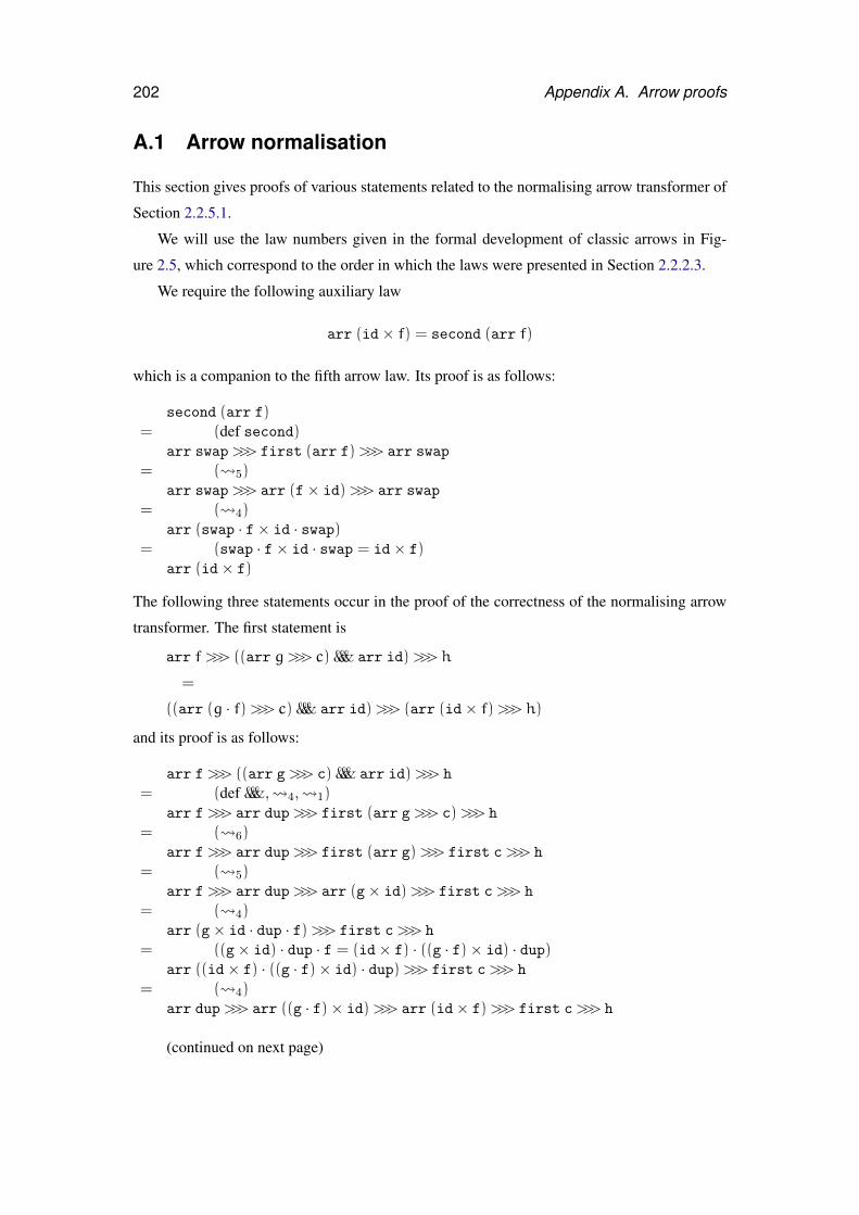
202 Appendix A. Arrow proofs
A.1 Arrow normalisation
This section gives proofs of various statements related to the normalising arrow transformer of
Section 2.2.5.1.
We will use the law numbers given in the formal development of classic arrows in Fig-
ure 2.5, which correspond to the order in which the laws were presented in Section 2.2.2.3.
We require the following auxiliary law
arr (id× f) = second (arr f)
which is a companion to the fifth arrow law. Its proof is as follows:
second (arr f)= (def second)
arr swap>>> first (arr f)>>> arr swap
= ( 5)arr swap>>> arr (f× id)>>> arr swap
= ( 4)arr (swap · f× id · swap)
= (swap · f× id · swap = id× f)arr (id× f)
The following three statements occur in the proof of the correctness of the normalising arrow
transformer. The first statement is
arr f >>> ((arr g >>> c) &&& arr id)>>> h
=
((arr (g · f)>>> c) &&& arr id)>>> (arr (id× f)>>> h)
and its proof is as follows:
arr f>>> ((arr g>>> c) &&& arr id)>>> h
= (def &&&, 4, 1)arr f>>> arr dup>>> first (arr g>>> c)>>> h
= ( 6)arr f>>> arr dup>>> first (arr g)>>> first c>>> h
= ( 5)arr f>>> arr dup>>> arr (g× id)>>> first c>>> h
= ( 4)arr (g× id · dup · f)>>> first c>>> h
= ((g× id) · dup · f = (id× f) · ((g · f)× id) · dup)arr ((id× f) · ((g · f)× id) · dup)>>> first c>>> h
= ( 4)arr dup>>> arr ((g · f)× id)>>> arr (id× f)>>> first c>>> h
(continued on next page)
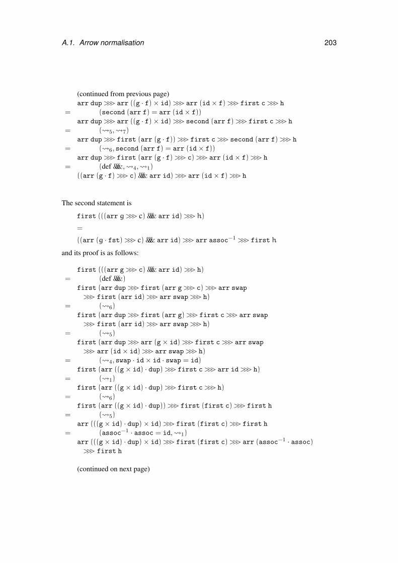
A.1. Arrow normalisation 203
(continued from previous page)arr dup>>> arr ((g · f)× id)>>> arr (id× f)>>> first c>>> h
= (second (arr f) = arr (id× f))arr dup>>> arr ((g · f)× id)>>> second (arr f)>>> first c>>> h
= ( 5, 7)arr dup>>> first (arr (g · f))>>> first c>>> second (arr f)>>> h
= ( 6, second (arr f) = arr (id× f))arr dup>>> first (arr (g · f)>>> c)>>> arr (id× f)>>> h
= (def &&&, 4, 1)((arr (g · f)>>> c) &&& arr id)>>> arr (id× f)>>> h
The second statement is
first (((arr g >>> c) &&& arr id)>>> h)
=
((arr (g · fst)>>> c) &&& arr id)>>> arr assoc−1 >>> first h
and its proof is as follows:
first (((arr g>>> c) &&& arr id)>>> h)= (def &&&)
first (arr dup>>> first (arr g>>> c)>>> arr swap
>>> first (arr id)>>> arr swap>>> h)= ( 6)
first (arr dup>>> first (arr g)>>> first c>>> arr swap
>>> first (arr id)>>> arr swap>>> h)= ( 5)
first (arr dup>>> arr (g× id)>>> first c>>> arr swap
>>> arr (id× id)>>> arr swap>>> h)= ( 4, swap · id× id · swap = id)
first (arr ((g× id) · dup)>>> first c>>> arr id>>> h)= ( 1)
first (arr ((g× id) · dup)>>> first c>>> h)= ( 6)
first (arr ((g× id) · dup))>>> first (first c)>>> first h
= ( 5)arr (((g× id) · dup)× id)>>> first (first c)>>> first h
= (assoc−1 · assoc = id, 1)arr (((g× id) · dup)× id)>>> first (first c)>>> arr (assoc−1 · assoc)>>> first h
(continued on next page)
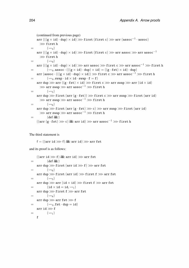
204 Appendix A. Arrow proofs
(continued from previous page)arr (((g× id) · dup)× id)>>> first (first c)>>> arr (assoc−1 · assoc)>>> first h
= ( 4)arr (((g× id) · dup)× id)>>> first (first c)>>> arr assoc>>> arr assoc−1
>>> first h
= ( 9)arr (((g× id) · dup)× id)>>> arr assoc>>> first c>>> arr assoc−1 >>> first h
= ( 4, assoc · (((g× id) · dup)× id) = ((g · fst)× id) · dup)arr (assoc · (((g× id) · dup)× id))>>> first c>>> arr assoc−1 >>> first h
= ( 4, swap · id× id · swap · f = f)arr dup>>> arr ((g · fst)× id)>>> first c>>> arr swap>>> arr (id× id)>>> arr swap>>> arr assoc−1 >>> first h
= ( 5)arr dup>>> first (arr (g · fst))>>> first c>>> arr swap>>> first (arr id)>>> arr swap>>> arr assoc−1 >>> first h
= ( 6)arr dup>>> first (arr (g · fst)>>> c)>>> arr swap>>> first (arr id)>>> arr swap>>> arr assoc−1 >>> first h
= (def &&&)((arr (g · fst)>>> c) &&& arr id)>>> arr assoc−1 >>> first h
The third statement is
f = ((arr id>>> f) &&& arr id)>>> arr fst
and its proof is as follows:
((arr id>>> f) &&& arr id)>>> arr fst
= (def &&&)arr dup>>> first (arr id>>> f)>>> arr fst
= ( 6)arr dup>>> first (arr id)>>> first f>>> arr fst
= ( 5)arr dup>>> arr (id× id)>>> first f>>> arr fst
= (id× id = id, 1)arr dup>>> first f>>> arr fst
= ( 8)arr dup>>> arr fst>>> f
= ( 4, fst · dup = id)arr id>>> f
= ( 1)f
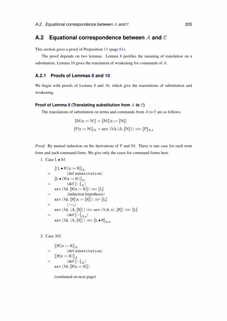
A.2. Equational correspondence between A and C 205
A.2 Equational correspondence between A and C
This section gives a proof of Proposition 11 (page 61).
The proof depends on two lemmas. Lemma 8 justifies the meaning of translation on a
substitution. Lemma 10 gives the translation of weakening for commands of A.
A.2.1 Proofs of Lemmas 8 and 10
We begin with proofs of Lemma 8 and 10, which give the translations of substitution and
weakening.
Proof of Lemma 8 (Translating substitution from A to C) .
The translations of substitution on terms and commands from A to C are as follows.
JM[x :=N]K = JMK[x := JNK]
JP[x :=N]K∆ = arr (λ∆.(∆, JNK))>>> JPK∆,x
Proof. By mutual induction on the derivations of P and M. There is one case for each term
form and each command form. We give only the cases for command forms here.
1. Case L •M
J(L • M)[x := N]K∆= (def substitution)
JL • (M[x := N])K∆= (def J−K∆)
arr (λ∆. JM[x := N]K)>>> JLK= (induction hypothesis)
arr (λ∆. JMK[x := JNK])>>> JLK= ( 4)
arr (λ∆. 〈∆, JNK〉)>>> arr (λ〈∆, x〉. JMK)>>> JLK= (def J−K∆,x)
arr (λ∆. 〈∆, JNK〉)>>> JL • MK∆,x
2. Case [M]
J[M][x := N]K∆= (def substitution)
J[M[x := N]]K∆= (def J−K∆)
arr (λ∆. JM[x := N]K)
(continued on next page)
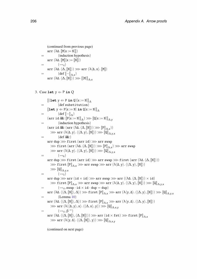
206 Appendix A. Arrow proofs
(continued from previous page)arr (λ∆. JM[x := N]K)
= (induction hypothesis)arr (λ∆. JMK[x := JNK])
= ( 4)arr (λ∆. 〈∆, JNK〉)>>> arr (λ〈∆, x〉. JMK)
= (def J−K∆,x)
arr (λ∆. 〈∆, JNK〉)>>> J[M]K∆,x
3. Case let y⇐ P in Q
J(let y⇐ P in Q)[x := N]K∆= (def substitution)
Jlet y⇐ P[x := N] in Q[x := N]K∆= (def J−K∆)
(arr id &&& JP[x := N]K∆)>>> JQ[x := N]K∆,y
= (induction hypothesis)(arr id &&& (arr (λ∆. 〈∆, JNK〉)>>> JPK∆,x))
>>> arr (λ〈∆, y〉. 〈〈∆, y〉, JNK〉)>>> JQK∆,y,x
= (def &&&)arr dup>>> first (arr id)>>> arr swap
>>> first (arr (λ∆. 〈∆, JNK〉)>>> JPK∆,x)>>> arr swap
>>> arr (λ〈∆, y〉. 〈〈∆, y〉, JNK〉)>>> JQK∆,y,x
= ( 6)arr dup>>> first (arr id)>>> arr swap>>> first (arr (λ∆. 〈∆, JNK〉))>>> first JPK∆,x >>> arr swap>>> arr (λ〈∆, y〉. 〈〈∆, y〉, JNK〉)>>> JQK∆,y,x
= ( 5)arr dup>>> arr (id× id)>>> arr swap>>> arr ((λ∆. 〈∆, JNK〉)× id)>>> first JPK∆,x >>> arr swap>>> arr (λ〈∆, y〉. 〈〈∆, y〉, JNK〉)>>> JQK∆,y,x
= ( 4, swap · id× id · dup = dup)arr (λ∆. 〈〈∆, JNK〉,∆〉)>>> first JPK∆,x >>> arr (λ〈y, ∆〉. 〈〈∆, y〉, JNK〉)>>> JQK∆,y,x
= (Lemma 10)arr (λ∆. 〈〈∆, JNK〉,∆〉)>>> first JPK∆,x >>> arr (λ〈y, ∆〉. 〈〈∆, y〉, JNK〉)>>> arr (λ〈〈∆, y〉, x〉. 〈〈∆, x〉, y〉)>>> JQK∆,x,y
= ( 4,β→)arr (λ∆. 〈〈∆, JNK〉, 〈∆, JNK〉〉)>>> arr (id× fst)>>> first JPK∆,x
>>> arr (λ〈y, ∆〉. 〈〈∆, JNK〉, y〉)>>> JQK∆,x,y
(continued on next page)
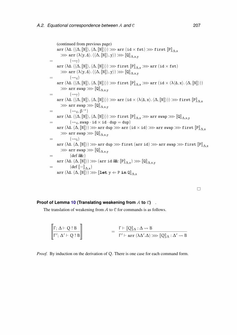
A.2. Equational correspondence between A and C 207
(continued from previous page)arr (λ∆. 〈〈∆, JNK〉, 〈∆, JNK〉〉)>>> arr (id× fst)>>> first JPK∆,x
>>> arr (λ〈y, ∆〉. 〈〈∆, JNK〉, y〉)>>> JQK∆,x,y
= ( 7)arr (λ∆. 〈〈∆, JNK〉, 〈∆, JNK〉〉)>>> first JPK∆,x >>> arr (id× fst)
>>> arr (λ〈y, ∆〉. 〈〈∆, JNK〉, y〉)>>> JQK∆,x,y
= ( 4)arr (λ∆. 〈〈∆, JNK〉, 〈∆, JNK〉〉)>>> first JPK∆,x >>> arr (id× (λ〈∆, x〉. 〈∆, JNK〉))>>> arr swap>>> JQK∆,x,y
= ( 7)arr (λ∆. 〈〈∆, JNK〉, 〈∆, JNK〉〉)>>> arr (id× (λ〈∆, x〉. 〈∆, JNK〉))>>> first JPK∆,x
>>> arr swap>>> JQK∆,x,y
= ( 4,β→)arr (λ∆. 〈〈∆, JNK〉, 〈∆, JNK〉〉)>>> first JPK∆,x >>> arr swap>>> JQK∆,x,y
= ( 4, swap · id× id · dup = dup)arr (λ∆. 〈∆, JNK〉)>>> arr dup>>> arr (id× id)>>> arr swap>>> first JPK∆,x
>>> arr swap>>> JQK∆,x,y
= ( 5)arr (λ∆. 〈∆, JNK〉)>>> arr dup>>> first (arr id)>>> arr swap>>> first JPK∆,x
>>> arr swap>>> JQK∆,x,y
= (def &&&)arr (λ∆. 〈∆, JNK〉)>>> (arr id &&& JPK∆,x)>>> JQK∆,x,y
= (def J−K∆,x)
arr (λ∆. 〈∆, JNK〉)>>> Jlet y⇐ P in QK∆,x
Proof of Lemma 10 (Translating weakening from A to C) .
The translation of weakening from A to C for commands is as follows.
u
vΓ ; ∆ ` Q ! B
Γ ′; ∆ ′ ` Q ! B
}
~ =Γ ` JQK∆ : ∆ B
Γ ′ ` arr (λ∆ ′.∆)>>> JQK∆ : ∆ ′ B
Proof. By induction on the derivation of Q. There is one case for each command form.
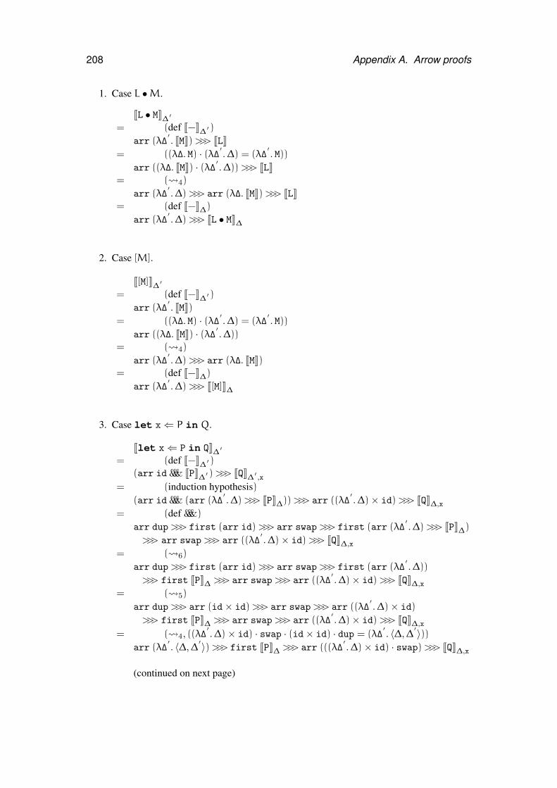
208 Appendix A. Arrow proofs
1. Case L •M.
JL • MK∆ ′= (def J−K∆ ′ )
arr (λ∆′. JMK)>>> JLK
= ((λ∆. M) · (λ∆ ′ .∆) = (λ∆′. M))
arr ((λ∆. JMK) · (λ∆ ′ .∆))>>> JLK= ( 4)
arr (λ∆′.∆)>>> arr (λ∆. JMK)>>> JLK
= (def J−K∆)arr (λ∆
′.∆)>>> JL • MK∆
2. Case [M].
J[M]K∆ ′= (def J−K∆ ′ )
arr (λ∆′. JMK)
= ((λ∆. M) · (λ∆ ′ .∆) = (λ∆′. M))
arr ((λ∆. JMK) · (λ∆ ′ .∆))= ( 4)
arr (λ∆′.∆)>>> arr (λ∆. JMK)
= (def J−K∆)arr (λ∆
′.∆)>>> J[M]K∆
3. Case let x⇐ P in Q.
Jlet x⇐ P in QK∆ ′= (def J−K∆ ′ )
(arr id &&& JPK∆ ′ )>>> JQK∆ ′ ,x= (induction hypothesis)
(arr id &&& (arr (λ∆′.∆)>>> JPK∆))>>> arr ((λ∆
′.∆)× id)>>> JQK∆,x
= (def &&&)
arr dup>>> first (arr id)>>> arr swap>>> first (arr (λ∆′.∆)>>> JPK∆)
>>> arr swap>>> arr ((λ∆′.∆)× id)>>> JQK∆,x
= ( 6)
arr dup>>> first (arr id)>>> arr swap>>> first (arr (λ∆′.∆))
>>> first JPK∆ >>> arr swap>>> arr ((λ∆′.∆)× id)>>> JQK∆,x
= ( 5)
arr dup>>> arr (id× id)>>> arr swap>>> arr ((λ∆′.∆)× id)
>>> first JPK∆ >>> arr swap>>> arr ((λ∆′.∆)× id)>>> JQK∆,x
= ( 4, ((λ∆′.∆)× id) · swap · (id× id) · dup = (λ∆
′. 〈∆,∆
′〉))arr (λ∆
′. 〈∆,∆
′〉)>>> first JPK∆ >>> arr (((λ∆′.∆)× id) · swap)>>> JQK∆,x
(continued on next page)
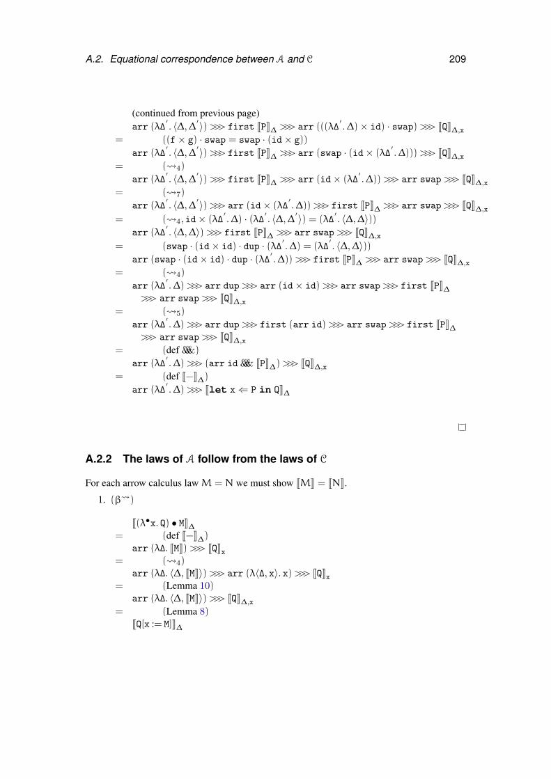
A.2. Equational correspondence between A and C 209
(continued from previous page)arr (λ∆
′. 〈∆,∆
′〉)>>> first JPK∆ >>> arr (((λ∆′.∆)× id) · swap)>>> JQK∆,x
= ((f× g) · swap = swap · (id× g))
arr (λ∆′. 〈∆,∆
′〉)>>> first JPK∆ >>> arr (swap · (id× (λ∆′.∆)))>>> JQK∆,x
= ( 4)
arr (λ∆′. 〈∆,∆
′〉)>>> first JPK∆ >>> arr (id× (λ∆′.∆))>>> arr swap>>> JQK∆,x
= ( 7)
arr (λ∆′. 〈∆,∆
′〉)>>> arr (id× (λ∆′.∆))>>> first JPK∆ >>> arr swap>>> JQK∆,x
= ( 4, id× (λ∆′.∆) · (λ∆ ′ . 〈∆,∆
′〉) = (λ∆′. 〈∆,∆〉))
arr (λ∆′. 〈∆,∆〉)>>> first JPK∆ >>> arr swap>>> JQK∆,x
= (swap · (id× id) · dup · (λ∆ ′ .∆) = (λ∆′. 〈∆,∆〉))
arr (swap · (id× id) · dup · (λ∆ ′ .∆))>>> first JPK∆ >>> arr swap>>> JQK∆,x
= ( 4)
arr (λ∆′.∆)>>> arr dup>>> arr (id× id)>>> arr swap>>> first JPK∆
>>> arr swap>>> JQK∆,x
= ( 5)
arr (λ∆′.∆)>>> arr dup>>> first (arr id)>>> arr swap>>> first JPK∆
>>> arr swap>>> JQK∆,x
= (def &&&)
arr (λ∆′.∆)>>> (arr id &&& JPK∆)>>> JQK∆,x
= (def J−K∆)arr (λ∆
′.∆)>>> Jlet x⇐ P in QK∆
A.2.2 The laws of A follow from the laws of C
For each arrow calculus lawM = N we must show JMK = JNK.
1. (β )
J(λ•x. Q) • MK∆= (def J−K∆)
arr (λ∆. JMK)>>> JQKx= ( 4)
arr (λ∆. 〈∆, JMK〉)>>> arr (λ〈∆, x〉. x)>>> JQKx= (Lemma 10)
arr (λ∆. 〈∆, JMK〉)>>> JQK∆,x
= (Lemma 8)JQ[x := M]K∆
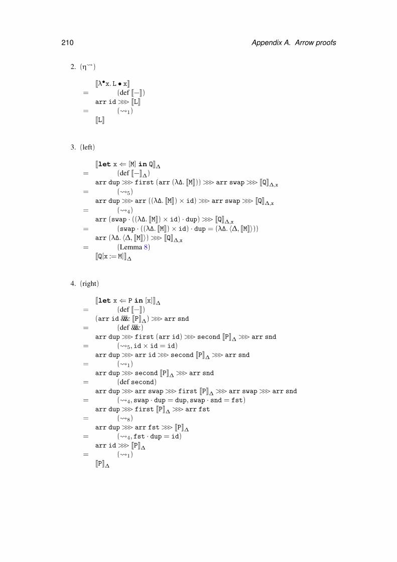
210 Appendix A. Arrow proofs
2. (η )
Jλ•x. L • xK= (def J−K)
arr id>>> JLK= ( 1)
JLK
3. (left)
Jlet x⇐ [M] in QK∆= (def J−K∆)
arr dup>>> first (arr (λ∆. JMK))>>> arr swap>>> JQK∆,x
= ( 5)arr dup>>> arr ((λ∆. JMK)× id)>>> arr swap>>> JQK∆,x
= ( 4)arr (swap · ((λ∆. JMK)× id) · dup)>>> JQK∆,x
= (swap · ((λ∆. JMK)× id) · dup = (λ∆. 〈∆, JMK〉))arr (λ∆. 〈∆, JMK〉)>>> JQK∆,x
= (Lemma 8)JQ[x := M]K∆
4. (right)
Jlet x⇐ P in [x]K∆= (def J−K)
(arr id &&& JPK∆)>>> arr snd
= (def &&&)arr dup>>> first (arr id)>>> second JPK∆ >>> arr snd
= ( 5, id× id = id)arr dup>>> arr id>>> second JPK∆ >>> arr snd
= ( 1)arr dup>>> second JPK∆ >>> arr snd
= (def second)arr dup>>> arr swap>>> first JPK∆ >>> arr swap>>> arr snd
= ( 4, swap · dup = dup, swap · snd = fst)arr dup>>> first JPK∆ >>> arr fst
= ( 8)arr dup>>> arr fst>>> JPK∆
= ( 4, fst · dup = id)arr id>>> JPK∆
= ( 1)JPK∆
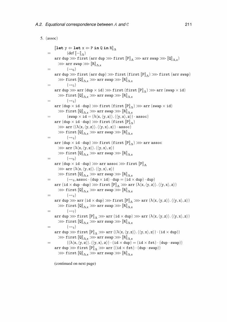
A.2. Equational correspondence between A and C 211
5. (assoc)
Jlet y⇐ let x⇐ P in Q in RK∆= (def J−K∆)
arr dup>>> first (arr dup>>> first JPK∆ >>> arr swap>>> JQK∆,x)
>>> arr swap>>> JRK∆,x
= ( 6)arr dup>>> first (arr dup)>>> first (first JPK∆)>>> first (arr swap)>>> first JQK∆,x >>> arr swap>>> JRK∆,x
= ( 5)arr dup>>> arr (dup× id)>>> first (first JPK∆)>>> arr (swap× id)>>> first JQK∆,x >>> arr swap>>> JRK∆,x
= ( 4)arr (dup× id · dup)>>> first (first JPK∆)>>> arr (swap× id)>>> first JQK∆,x >>> arr swap>>> JRK∆,x
= (swap× id = (λ〈x, 〈y, z〉〉. 〈〈y, x〉, z〉) · assoc)arr (dup× id · dup)>>> first (first JPK∆)>>> arr ((λ〈x, 〈y, z〉〉. 〈〈y, x〉, z〉) · assoc)>>> first JQK∆,x >>> arr swap>>> JRK∆,x
= ( 4)arr (dup× id · dup)>>> first (first JPK∆)>>> arr assoc
>>> arr (λ〈x, 〈y, z〉〉. 〈〈y, x〉, z〉)>>> first JQK∆,x >>> arr swap>>> JRK∆,x
= ( 9)arr (dup× id · dup)>>> arr assoc>>> first JPK∆>>> arr (λ〈x, 〈y, z〉〉. 〈〈y, x〉, z〉)>>> first JQK∆,x >>> arr swap>>> JRK∆,x
= ( 4, assoc · (dup× id) · dup = (id× dup) · dup)arr (id× dup · dup)>>> first JPK∆ >>> arr (λ〈x, 〈y, z〉〉. 〈〈y, x〉, z〉)>>> first JQK∆,x >>> arr swap>>> JRK∆,x
= ( 4)arr dup>>> arr (id× dup)>>> first JPK∆ >>> arr (λ〈x, 〈y, z〉〉. 〈〈y, x〉, z〉)>>> first JQK∆,x >>> arr swap>>> JRK∆,x
= ( 7)arr dup>>> first JPK∆ >>> arr (id× dup)>>> arr (λ〈x, 〈y, z〉〉. 〈〈y, x〉, z〉)>>> first JQK∆,x >>> arr swap>>> JRK∆,x
= ( 4)arr dup>>> first JPK∆ >>> arr ((λ〈x, 〈y, z〉〉. 〈〈y, x〉, z〉) · (id× dup))>>> first JQK∆,x >>> arr swap>>> JRK∆,x
= ((λ〈x, 〈y, z〉〉. 〈〈y, x〉, z〉) · (id× dup) = (id× fst) · (dup · swap))arr dup>>> first JPK∆ >>> arr ((id× fst) · (dup · swap))>>> first JQK∆,x >>> arr swap>>> JRK∆,x
(continued on next page)
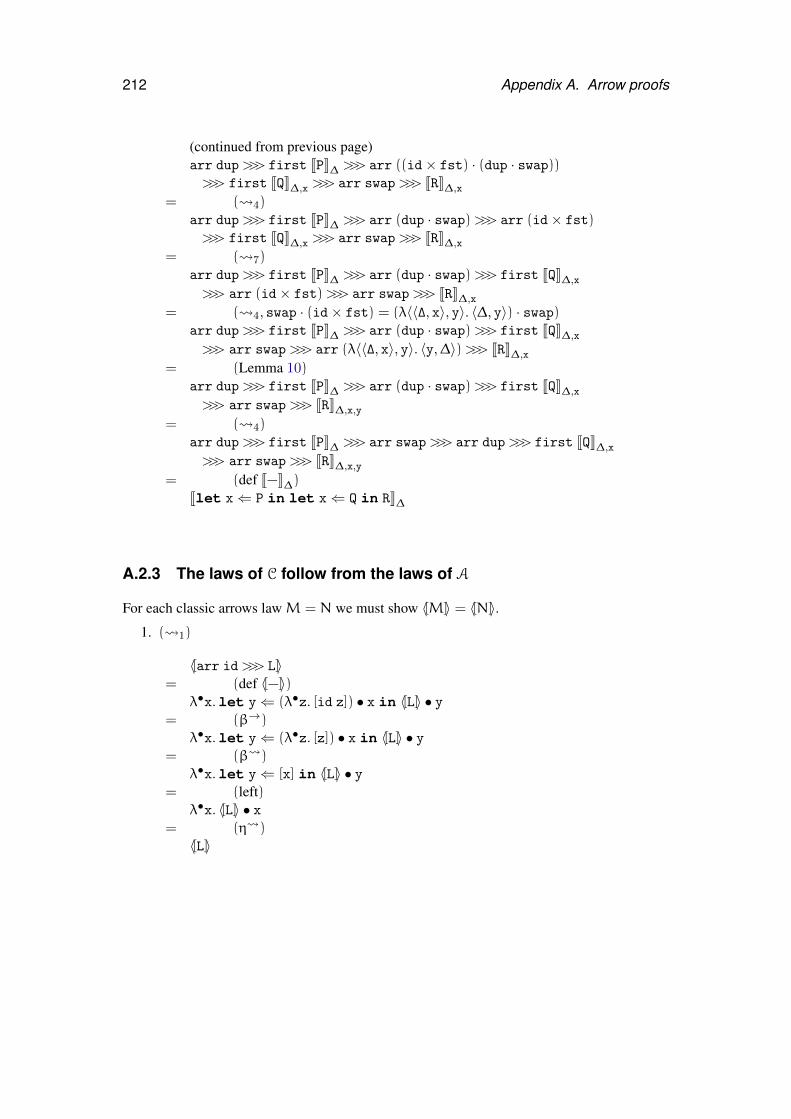
212 Appendix A. Arrow proofs
(continued from previous page)arr dup>>> first JPK∆ >>> arr ((id× fst) · (dup · swap))>>> first JQK∆,x >>> arr swap>>> JRK∆,x
= ( 4)arr dup>>> first JPK∆ >>> arr (dup · swap)>>> arr (id× fst)>>> first JQK∆,x >>> arr swap>>> JRK∆,x
= ( 7)arr dup>>> first JPK∆ >>> arr (dup · swap)>>> first JQK∆,x
>>> arr (id× fst)>>> arr swap>>> JRK∆,x
= ( 4, swap · (id× fst) = (λ〈〈∆, x〉, y〉. 〈∆, y〉) · swap)arr dup>>> first JPK∆ >>> arr (dup · swap)>>> first JQK∆,x
>>> arr swap>>> arr (λ〈〈∆, x〉, y〉. 〈y,∆〉)>>> JRK∆,x
= (Lemma 10)arr dup>>> first JPK∆ >>> arr (dup · swap)>>> first JQK∆,x
>>> arr swap>>> JRK∆,x,y
= ( 4)arr dup>>> first JPK∆ >>> arr swap>>> arr dup>>> first JQK∆,x
>>> arr swap>>> JRK∆,x,y
= (def J−K∆)Jlet x⇐ P in let x⇐ Q in RK∆
A.2.3 The laws of C follow from the laws of A
For each classic arrows lawM = N we must show 〈[M]〉 = 〈[N]〉.1. ( 1)
〈[arr id>>> L]〉= (def 〈[−]〉)
λ•x.let y⇐ (λ•z. [id z]) • x in 〈[L]〉 • y= (β→)
λ•x.let y⇐ (λ•z. [z]) • x in 〈[L]〉 • y= (β )
λ•x.let y⇐ [x] in 〈[L]〉 • y= (left)
λ•x. 〈[L]〉 • x= (η )〈[L]〉
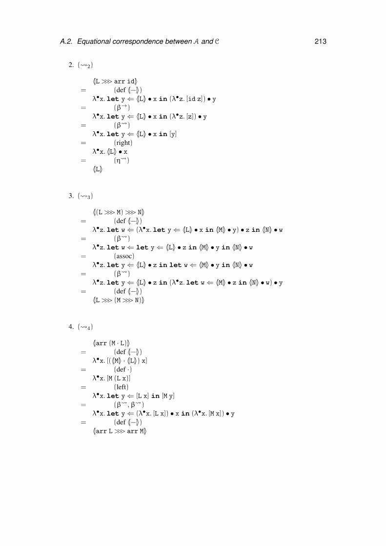
A.2. Equational correspondence between A and C 213
2. ( 2)
〈[L>>> arr id]〉= (def 〈[−]〉)
λ•x.let y⇐ 〈[L]〉 • x in (λ•z. [id z]) • y= (β→)
λ•x.let y⇐ 〈[L]〉 • x in (λ•z. [z]) • y= (β )
λ•x.let y⇐ 〈[L]〉 • x in [y]= (right)
λ•x. 〈[L]〉 • x= (η )〈[L]〉
3. ( 3)
〈[(L>>> M)>>> N]〉= (def 〈[−]〉)
λ•z.let w⇐ (λ•x.let y⇐ 〈[L]〉 • x in 〈[M]〉 • y) • z in 〈[N]〉 • w= (β )
λ•z.let w⇐ let y⇐ 〈[L]〉 • z in 〈[M]〉 • y in 〈[N]〉 • w= (assoc)
λ•z.let y⇐ 〈[L]〉 • z in let w⇐ 〈[M]〉 • y in 〈[N]〉 • w= (β )
λ•z.let y⇐ 〈[L]〉 • z in (λ•z.let w⇐ 〈[M]〉 • z in 〈[N]〉 • w) • y= (def 〈[−]〉)〈[L>>> (M>>> N)]〉
4. ( 4)
〈[arr (M · L)]〉= (def 〈[−]〉)
λ•x. [(〈[M]〉 · 〈[L]〉) x]= (def ·)
λ•x. [M (L x)]= (left)
λ•x.let y⇐ [L x] in [M y]= (β ,β )
λ•x.let y⇐ (λ•x. [L x]) • x in (λ•x. [M x]) • y= (def 〈[−]〉)〈[arr L>>> arr M]〉
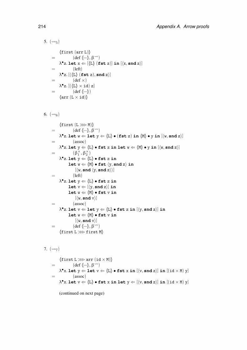
214 Appendix A. Arrow proofs
5. ( 5)
〈[first (arr L)]〉= (def 〈[−]〉,β )
λ•z.let x⇐ [〈[L]〉 (fst z)] in [〈x,snd z〉]= (left)
λ•z. [〈〈[L]〉 (fst z),snd z〉]= (def ×)
λ•z. [(〈[L]〉 × id) z]= (def 〈[−]〉)〈[arr (L× id)]〉
6. ( 6)
〈[first (L>>> M)]〉= (def 〈[−]〉,β )
λ•z.let w⇐ let y⇐ 〈[L]〉 • (fst z) in 〈[M]〉 • y in [〈w,snd z〉]= (assoc)
λ•z.let y⇐ 〈[L]〉 • fst z in let w⇐ 〈[M]〉 • y in [〈w,snd z〉]= (β×1 ,β×2 )
λ•z.let y⇐ 〈[L]〉 • fst z inlet w⇐ 〈[M]〉 • fst 〈y,snd z〉 in
[〈w,snd 〈y,snd z〉〉]= (left)
λ•z.let y⇐ 〈[L]〉 • fst z inlet v⇐ [〈y,snd z〉] inlet w⇐ 〈[M]〉 • fst v in
[〈w,snd v〉]= (assoc)
λ•z.let v⇐ let y⇐ 〈[L]〉 • fst z in [〈y,snd z〉] inlet w⇐ 〈[M]〉 • fst v in
[〈w,snd v〉]= (def 〈[−]〉,β )〈[first L>>> first M]〉
7. ( 7)
〈[first L>>> arr (id× M)]〉= (def 〈[−]〉,β )
λ•x.let y⇐ let v⇐ 〈[L]〉 • fst x in [〈v,snd z〉] in [(id× M) y]= (assoc)
λ•x.let v⇐ 〈[L]〉 • fst x in let y⇐ [〈v,snd z〉] in [(id× M) y]
(continued on next page)
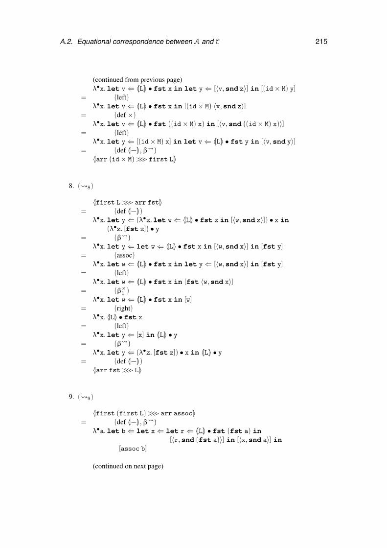
A.2. Equational correspondence between A and C 215
(continued from previous page)λ•x.let v⇐ 〈[L]〉 • fst x in let y⇐ [〈v,snd z〉] in [(id× M) y]
= (left)λ•x.let v⇐ 〈[L]〉 • fst x in [(id× M) 〈v,snd z〉]
= (def ×)λ•x.let v⇐ 〈[L]〉 • fst ((id× M) x) in [〈v,snd ((id× M) x)〉]
= (left)λ•x.let y⇐ [(id× M) x] in let v⇐ 〈[L]〉 • fst y in [〈v,snd y〉]
= (def 〈[−]〉,β )〈[arr (id× M)>>> first L]〉
8. ( 8)
〈[first L>>> arr fst]〉= (def 〈[−]〉)
λ•x.let y⇐ (λ•z.let w⇐ 〈[L]〉 • fst z in [〈w,snd z〉]) • x in(λ•z. [fst z]) • y
= (β )λ•x.let y⇐ let w⇐ 〈[L]〉 • fst x in [〈w,snd x〉] in [fst y]
= (assoc)λ•x.let w⇐ 〈[L]〉 • fst x in let y⇐ [〈w,snd x〉] in [fst y]
= (left)λ•x.let w⇐ 〈[L]〉 • fst x in [fst 〈w,snd x〉]
= (β×1 )λ•x.let w⇐ 〈[L]〉 • fst x in [w]
= (right)λ•x. 〈[L]〉 • fst x
= (left)λ•x.let y⇐ [x] in 〈[L]〉 • y
= (β )λ•x.let y⇐ (λ•z. [fst z]) • x in 〈[L]〉 • y
= (def 〈[−]〉)〈[arr fst>>> L]〉
9. ( 9)
〈[first (first L)>>> arr assoc]〉= (def 〈[−]〉,β )
λ•a.let b⇐ let x⇐ let r⇐ 〈[L]〉 • fst (fst a) in[〈r,snd (fst a)〉] in [〈x,snd a〉] in
[assoc b]
(continued on next page)
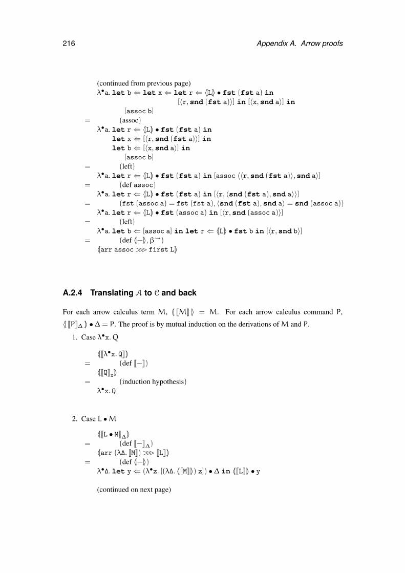
216 Appendix A. Arrow proofs
(continued from previous page)λ•a.let b⇐ let x⇐ let r⇐ 〈[L]〉 • fst (fst a) in
[〈r,snd (fst a)〉] in [〈x,snd a〉] in[assoc b]
= (assoc)λ•a.let r⇐ 〈[L]〉 • fst (fst a) in
let x⇐ [〈r,snd (fst a)〉] inlet b⇐ [〈x,snd a〉] in
[assoc b]= (left)
λ•a.let r⇐ 〈[L]〉 • fst (fst a) in [assoc 〈〈r,snd (fst a)〉,snd a〉]= (def assoc)
λ•a.let r⇐ 〈[L]〉 • fst (fst a) in [〈r, 〈snd (fst a),snd a〉〉]= (fst (assoc a) = fst (fst a), 〈snd (fst a),snd a〉 = snd (assoc a))
λ•a.let r⇐ 〈[L]〉 • fst (assoc a) in [〈r,snd (assoc a)〉]= (left)
λ•a.let b⇐ [assoc a] in let r⇐ 〈[L]〉 • fst b in [〈r,snd b〉]= (def 〈[−]〉,β )〈[arr assoc>>> first L]〉
A.2.4 Translating A to C and back
For each arrow calculus term M, 〈[ JMK ]〉 = M. For each arrow calculus command P,
〈[ JPK∆ ]〉 • ∆ = P. The proof is by mutual induction on the derivations ofM and P.
1. Case λ•x.Q
〈[Jλ•x. QK]〉= (def J−K)〈[JQKx]〉
= (induction hypothesis)λ•x. Q
2. Case L •M
〈[JL • MK∆]〉= (def J−K∆)〈[arr (λ∆. JMK)>>> JLK]〉
= (def 〈[−]〉)λ•∆.let y⇐ (λ•z. [(λ∆. 〈[JMK]〉) z]) • ∆ in 〈[JLK]〉 • y
(continued on next page)
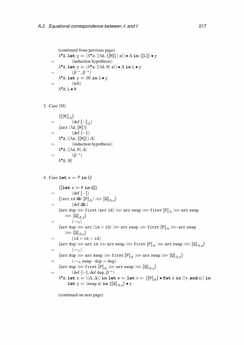
A.2. Equational correspondence between A and C 217
(continued from previous page)λ•∆.let y⇐ (λ•z. [(λ∆. 〈[JMK]〉) z]) • ∆ in 〈[JLK]〉 • y
= (induction hypothesis)λ•∆.let y⇐ (λ•z. [(λ∆. M) z]) • ∆ in L • y
= (β ,β→)λ•∆.let y⇐ [M] in L • y
= (left)λ•∆. L • M
3. Case [M]
〈[J[M]K∆]〉= (def J−K∆)〈[arr (λ∆. JMK)]〉
= (def 〈[−]〉)λ•∆. [(λ∆. 〈[JMK]〉) ∆]
= (induction hypothesis)λ•∆. [(λ∆. M) ∆]
= (β→)λ•∆. [M]
4. Case let x⇐ P in Q
〈[Jlet x⇐ P in QK]〉= (def J−K)〈[(arr id &&& JPK∆)>>> JQK∆,x]〉
= (def &&&)〈[arr dup>>> first (arr id)>>> arr swap>>> first JPK∆ >>> arr swap
>>> JQK∆,x]〉= ( 5)〈[arr dup>>> arr (id× id)>>> arr swap>>> first JPK∆ >>> arr swap
>>> JQK∆,x]〉= (id× id = id)〈[arr dup>>> arr id>>> arr swap>>> first JPK∆ >>> arr swap>>> JQK∆,x]〉
= ( 1)〈[arr dup>>> arr swap>>> first JPK∆ >>> arr swap>>> JQK∆,x]〉
= ( 4, swap · dup = dup)〈[arr dup>>> first JPK∆ >>> arr swap>>> JQK∆,x]〉
= (def 〈[−]〉, def dup,β )λ•∆.let x⇐ [〈∆,∆〉] in let w⇐ let v⇐ 〈[JPK∆]〉 • fst x in [〈v,snd x〉] in
let y⇐ [swap w] in 〈[JQK∆,x]〉 • y
(continued on next page)
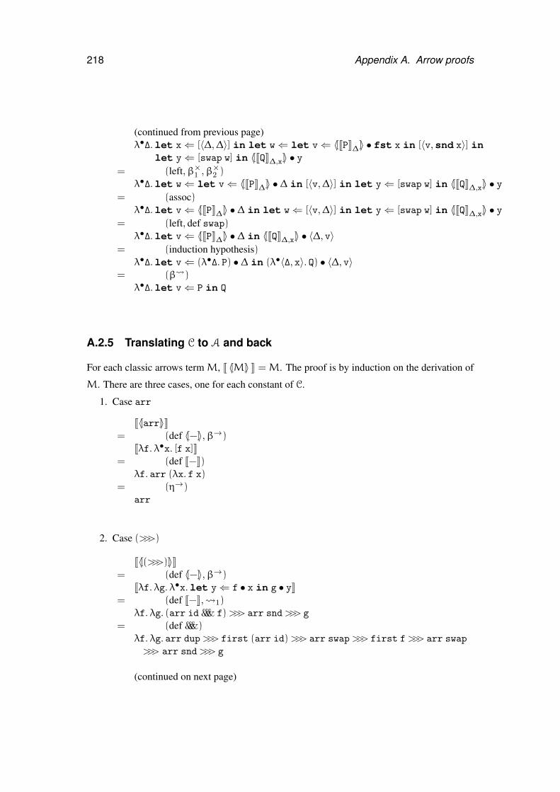
218 Appendix A. Arrow proofs
(continued from previous page)λ•∆.let x⇐ [〈∆,∆〉] in let w⇐ let v⇐ 〈[JPK∆]〉 • fst x in [〈v,snd x〉] in
let y⇐ [swap w] in 〈[JQK∆,x]〉 • y= (left,β×1 ,β×2 )
λ•∆.let w⇐ let v⇐ 〈[JPK∆]〉 • ∆ in [〈v,∆〉] in let y⇐ [swap w] in 〈[JQK∆,x]〉 • y= (assoc)
λ•∆.let v⇐ 〈[JPK∆]〉 • ∆ in let w⇐ [〈v,∆〉] in let y⇐ [swap w] in 〈[JQK∆,x]〉 • y= (left, def swap)
λ•∆.let v⇐ 〈[JPK∆]〉 • ∆ in 〈[JQK∆,x]〉 • 〈∆, v〉= (induction hypothesis)
λ•∆.let v⇐ (λ•∆. P) • ∆ in (λ•〈∆, x〉. Q) • 〈∆, v〉= (β )
λ•∆.let v⇐ P in Q
A.2.5 Translating C to A and back
For each classic arrows term M, J 〈[M]〉 K =M. The proof is by induction on the derivation of
M. There are three cases, one for each constant of C.
1. Case arr
J〈[arr]〉K= (def 〈[−]〉,β→)
Jλf. λ•x. [f x]K= (def J−K)
λf. arr (λx. f x)= (η→)
arr
2. Case (>>>)
J〈[(>>>)]〉K= (def 〈[−]〉,β→)
Jλf. λg. λ•x.let y⇐ f • x in g • yK= (def J−K, 1)
λf. λg. (arr id &&& f)>>> arr snd>>> g
= (def &&&)λf. λg. arr dup>>> first (arr id)>>> arr swap>>> first f>>> arr swap
>>> arr snd>>> g
(continued on next page)
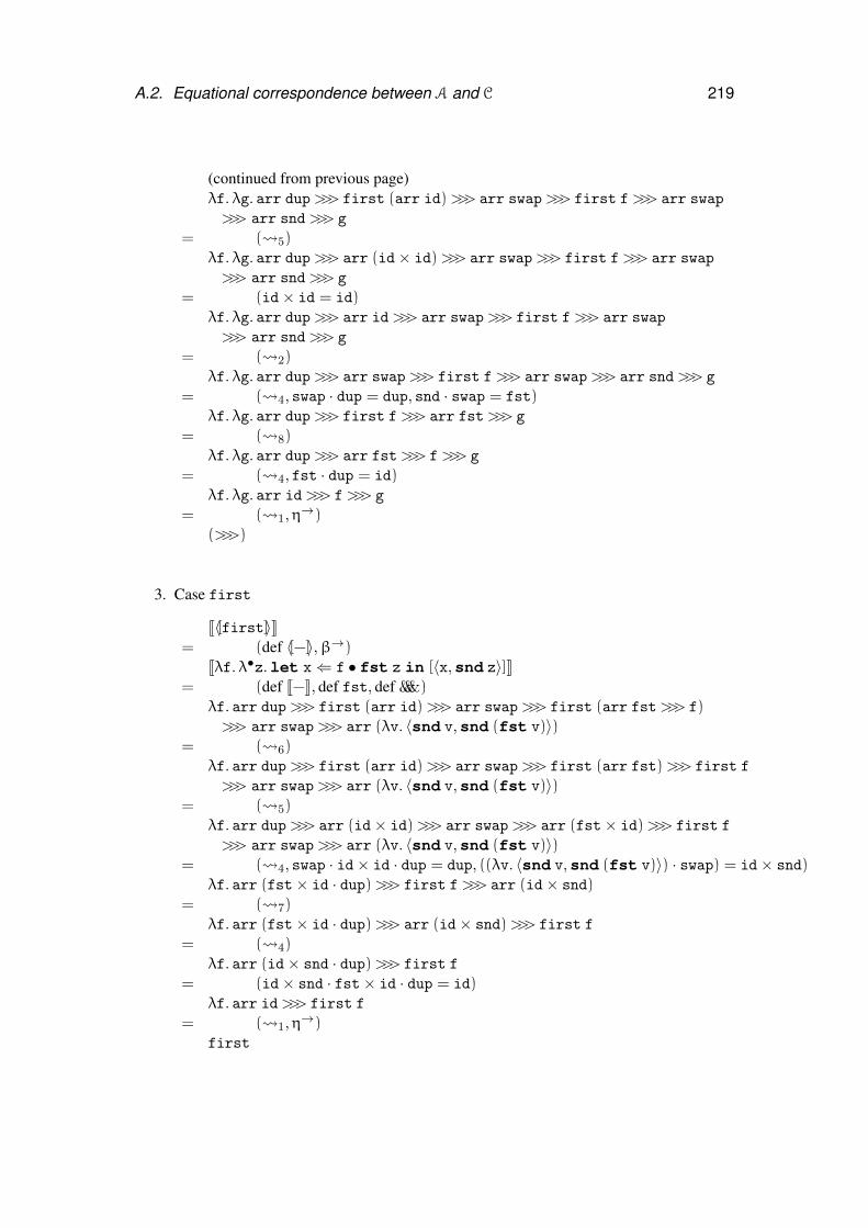
A.2. Equational correspondence between A and C 219
(continued from previous page)λf. λg. arr dup>>> first (arr id)>>> arr swap>>> first f>>> arr swap
>>> arr snd>>> g
= ( 5)λf. λg. arr dup>>> arr (id× id)>>> arr swap>>> first f>>> arr swap
>>> arr snd>>> g
= (id× id = id)λf. λg. arr dup>>> arr id>>> arr swap>>> first f>>> arr swap
>>> arr snd>>> g
= ( 2)λf. λg. arr dup>>> arr swap>>> first f>>> arr swap>>> arr snd>>> g
= ( 4, swap · dup = dup, snd · swap = fst)λf. λg. arr dup>>> first f>>> arr fst>>> g
= ( 8)λf. λg. arr dup>>> arr fst>>> f>>> g
= ( 4, fst · dup = id)λf. λg. arr id>>> f>>> g
= ( 1,η→)(>>>)
3. Case first
J〈[first]〉K= (def 〈[−]〉,β→)
Jλf. λ•z.let x⇐ f • fst z in [〈x,snd z〉]K= (def J−K, def fst, def &&&)
λf. arr dup>>> first (arr id)>>> arr swap>>> first (arr fst>>> f)>>> arr swap>>> arr (λv. 〈snd v,snd (fst v)〉)
= ( 6)λf. arr dup>>> first (arr id)>>> arr swap>>> first (arr fst)>>> first f
>>> arr swap>>> arr (λv. 〈snd v,snd (fst v)〉)= ( 5)
λf. arr dup>>> arr (id× id)>>> arr swap>>> arr (fst× id)>>> first f
>>> arr swap>>> arr (λv. 〈snd v,snd (fst v)〉)= ( 4, swap · id× id · dup = dup, ((λv. 〈snd v,snd (fst v)〉) · swap) = id× snd)
λf. arr (fst× id · dup)>>> first f>>> arr (id× snd)= ( 7)
λf. arr (fst× id · dup)>>> arr (id× snd)>>> first f
= ( 4)λf. arr (id× snd · dup)>>> first f
= (id× snd · fst× id · dup = id)λf. arr id>>> first f
= ( 1,η→)first
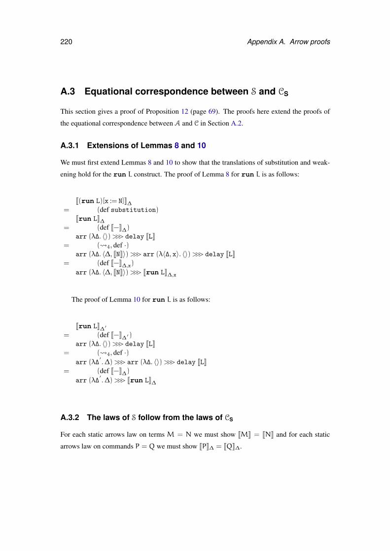
220 Appendix A. Arrow proofs
A.3 Equational correspondence between S and CS
This section gives a proof of Proposition 12 (page 69). The proofs here extend the proofs of
the equational correspondence between A and C in Section A.2.
A.3.1 Extensions of Lemmas 8 and 10
We must first extend Lemmas 8 and 10 to show that the translations of substitution and weak-
ening hold for the run L construct. The proof of Lemma 8 for run L is as follows:
J(run L)[x := N]K∆= (def substitution)
Jrun LK∆= (def J−K∆)
arr (λ∆. 〈〉)>>> delay JLK= ( 4, def ·)
arr (λ∆. 〈∆, JNK〉)>>> arr (λ〈∆, x〉. 〈〉)>>> delay JLK= (def J−K∆,x)
arr (λ∆. 〈∆, JNK〉)>>> Jrun LK∆,x
The proof of Lemma 10 for run L is as follows:
Jrun LK∆ ′= (def J−K∆ ′ )
arr (λ∆. 〈〉)>>> delay JLK= ( 4, def ·)
arr (λ∆′.∆)>>> arr (λ∆. 〈〉)>>> delay JLK
= (def J−K∆)arr (λ∆
′.∆)>>> Jrun LK∆
A.3.2 The laws of S follow from the laws of CS
For each static arrows law on terms M = N we must show JMK = JNK and for each static
arrows law on commands P = Q we must show JPK∆ = JQK∆.
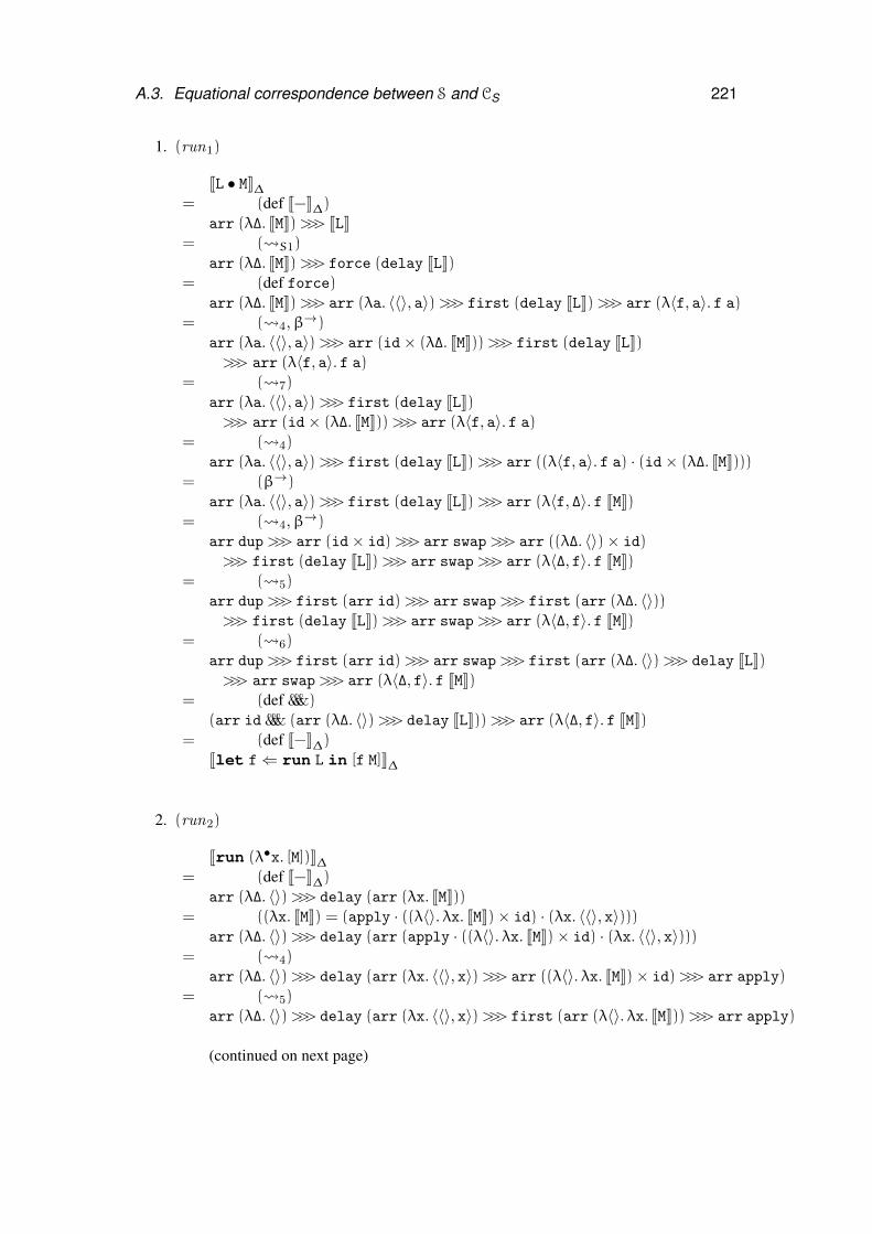
A.3. Equational correspondence between S and CS 221
1. (run1)
JL • MK∆= (def J−K∆)
arr (λ∆. JMK)>>> JLK= ( S1)
arr (λ∆. JMK)>>> force (delay JLK)= (def force)
arr (λ∆. JMK)>>> arr (λa. 〈〈〉, a〉)>>> first (delay JLK)>>> arr (λ〈f, a〉. f a)= ( 4,β→)
arr (λa. 〈〈〉, a〉)>>> arr (id× (λ∆. JMK))>>> first (delay JLK)>>> arr (λ〈f, a〉. f a)
= ( 7)arr (λa. 〈〈〉, a〉)>>> first (delay JLK)>>> arr (id× (λ∆. JMK))>>> arr (λ〈f, a〉. f a)
= ( 4)arr (λa. 〈〈〉, a〉)>>> first (delay JLK)>>> arr ((λ〈f, a〉. f a) · (id× (λ∆. JMK)))
= (β→)arr (λa. 〈〈〉, a〉)>>> first (delay JLK)>>> arr (λ〈f, ∆〉. f JMK)
= ( 4,β→)arr dup>>> arr (id× id)>>> arr swap>>> arr ((λ∆. 〈〉)× id)>>> first (delay JLK)>>> arr swap>>> arr (λ〈∆, f〉. f JMK)
= ( 5)arr dup>>> first (arr id)>>> arr swap>>> first (arr (λ∆. 〈〉))>>> first (delay JLK)>>> arr swap>>> arr (λ〈∆, f〉. f JMK)
= ( 6)arr dup>>> first (arr id)>>> arr swap>>> first (arr (λ∆. 〈〉)>>> delay JLK)>>> arr swap>>> arr (λ〈∆, f〉. f JMK)
= (def &&&)(arr id &&& (arr (λ∆. 〈〉)>>> delay JLK))>>> arr (λ〈∆, f〉. f JMK)
= (def J−K∆)Jlet f⇐ run L in [f M]K∆
2. (run2)
Jrun (λ•x. [M])K∆= (def J−K∆)
arr (λ∆. 〈〉)>>> delay (arr (λx. JMK))= ((λx. JMK) = (apply · ((λ〈〉. λx. JMK)× id) · (λx. 〈〈〉, x〉)))
arr (λ∆. 〈〉)>>> delay (arr (apply · ((λ〈〉. λx. JMK)× id) · (λx. 〈〈〉, x〉)))= ( 4)
arr (λ∆. 〈〉)>>> delay (arr (λx. 〈〈〉, x〉)>>> arr ((λ〈〉. λx. JMK)× id)>>> arr apply)= ( 5)
arr (λ∆. 〈〉)>>> delay (arr (λx. 〈〈〉, x〉)>>> first (arr (λ〈〉. λx. JMK))>>> arr apply)
(continued on next page)
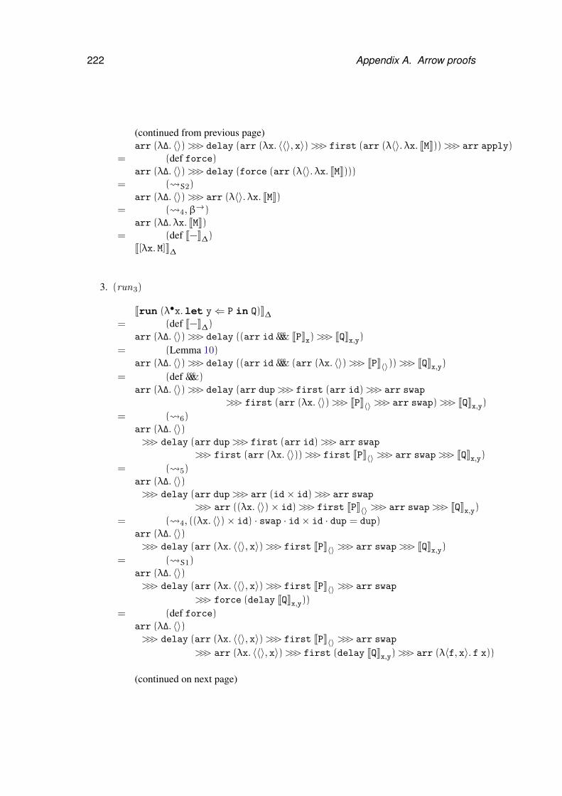
222 Appendix A. Arrow proofs
(continued from previous page)arr (λ∆. 〈〉)>>> delay (arr (λx. 〈〈〉, x〉)>>> first (arr (λ〈〉. λx. JMK))>>> arr apply)
= (def force)arr (λ∆. 〈〉)>>> delay (force (arr (λ〈〉. λx. JMK)))
= ( S2)arr (λ∆. 〈〉)>>> arr (λ〈〉. λx. JMK)
= ( 4,β→)arr (λ∆. λx. JMK)
= (def J−K∆)J[λx. M]K∆
3. (run3)
Jrun (λ•x.let y⇐ P in Q)K∆= (def J−K∆)
arr (λ∆. 〈〉)>>> delay ((arr id &&& JPKx)>>> JQKx,y)
= (Lemma 10)arr (λ∆. 〈〉)>>> delay ((arr id &&& (arr (λx. 〈〉)>>> JPK〈〉))>>> JQKx,y)
= (def &&&)arr (λ∆. 〈〉)>>> delay (arr dup>>> first (arr id)>>> arr swap
>>> first (arr (λx. 〈〉)>>> JPK〈〉 >>> arr swap)>>> JQKx,y)
= ( 6)arr (λ∆. 〈〉)>>> delay (arr dup>>> first (arr id)>>> arr swap
>>> first (arr (λx. 〈〉))>>> first JPK〈〉 >>> arr swap>>> JQKx,y)
= ( 5)arr (λ∆. 〈〉)>>> delay (arr dup>>> arr (id× id)>>> arr swap
>>> arr ((λx. 〈〉)× id)>>> first JPK〈〉 >>> arr swap>>> JQKx,y)
= ( 4, ((λx. 〈〉)× id) · swap · id× id · dup = dup)arr (λ∆. 〈〉)>>> delay (arr (λx. 〈〈〉, x〉)>>> first JPK〈〉 >>> arr swap>>> JQKx,y)
= ( S1)arr (λ∆. 〈〉)>>> delay (arr (λx. 〈〈〉, x〉)>>> first JPK〈〉 >>> arr swap
>>> force (delay JQKx,y))
= (def force)arr (λ∆. 〈〉)>>> delay (arr (λx. 〈〈〉, x〉)>>> first JPK〈〉 >>> arr swap
>>> arr (λx. 〈〈〉, x〉)>>> first (delay JQKx,y)>>> arr (λ〈f, x〉. f x))
(continued on next page)
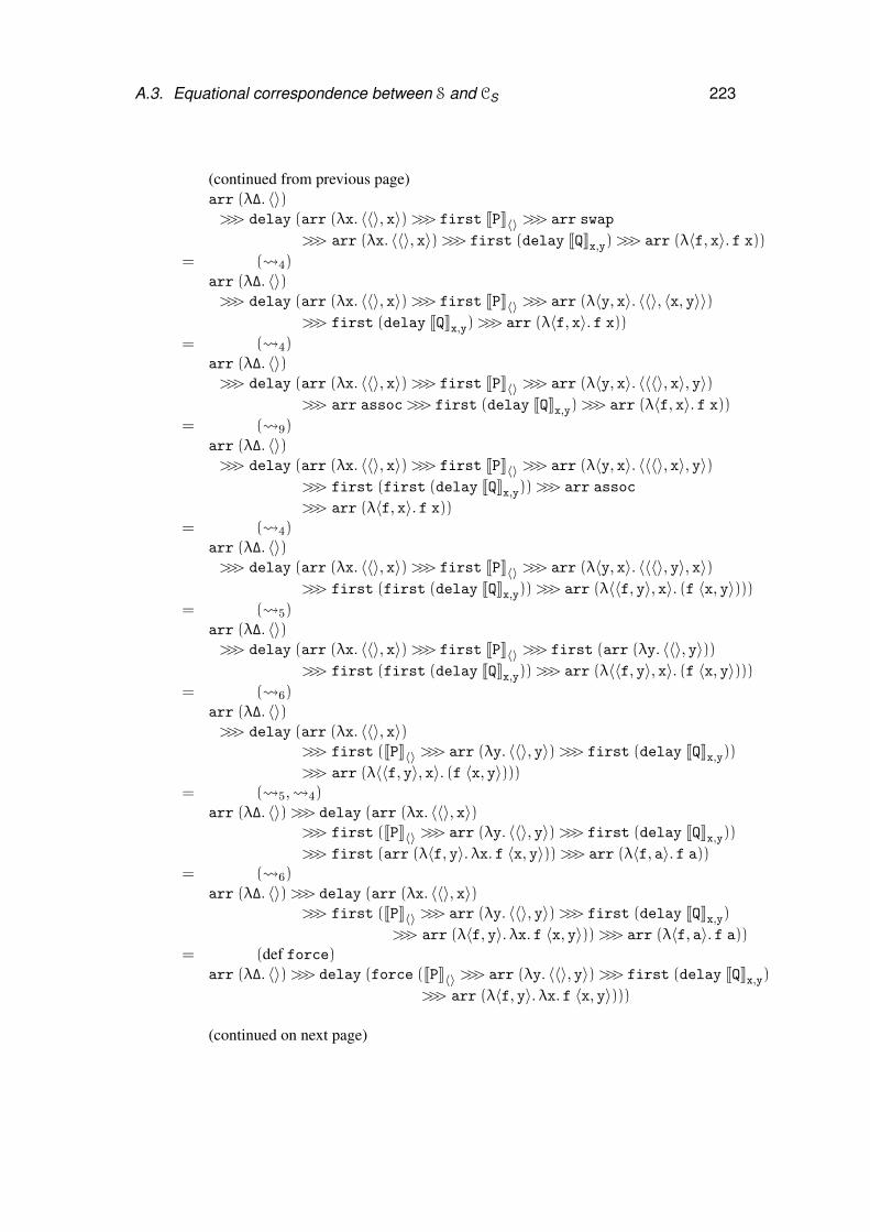
A.3. Equational correspondence between S and CS 223
(continued from previous page)arr (λ∆. 〈〉)>>> delay (arr (λx. 〈〈〉, x〉)>>> first JPK〈〉 >>> arr swap
>>> arr (λx. 〈〈〉, x〉)>>> first (delay JQKx,y)>>> arr (λ〈f, x〉. f x))= ( 4)
arr (λ∆. 〈〉)>>> delay (arr (λx. 〈〈〉, x〉)>>> first JPK〈〉 >>> arr (λ〈y, x〉. 〈〈〉, 〈x, y〉〉)
>>> first (delay JQKx,y)>>> arr (λ〈f, x〉. f x))= ( 4)
arr (λ∆. 〈〉)>>> delay (arr (λx. 〈〈〉, x〉)>>> first JPK〈〉 >>> arr (λ〈y, x〉. 〈〈〈〉, x〉, y〉)
>>> arr assoc>>> first (delay JQKx,y)>>> arr (λ〈f, x〉. f x))= ( 9)
arr (λ∆. 〈〉)>>> delay (arr (λx. 〈〈〉, x〉)>>> first JPK〈〉 >>> arr (λ〈y, x〉. 〈〈〈〉, x〉, y〉)
>>> first (first (delay JQKx,y))>>> arr assoc
>>> arr (λ〈f, x〉. f x))= ( 4)
arr (λ∆. 〈〉)>>> delay (arr (λx. 〈〈〉, x〉)>>> first JPK〈〉 >>> arr (λ〈y, x〉. 〈〈〈〉, y〉, x〉)
>>> first (first (delay JQKx,y))>>> arr (λ〈〈f, y〉, x〉. (f 〈x, y〉)))= ( 5)
arr (λ∆. 〈〉)>>> delay (arr (λx. 〈〈〉, x〉)>>> first JPK〈〉 >>> first (arr (λy. 〈〈〉, y〉))
>>> first (first (delay JQKx,y))>>> arr (λ〈〈f, y〉, x〉. (f 〈x, y〉)))= ( 6)
arr (λ∆. 〈〉)>>> delay (arr (λx. 〈〈〉, x〉)
>>> first (JPK〈〉 >>> arr (λy. 〈〈〉, y〉)>>> first (delay JQKx,y))
>>> arr (λ〈〈f, y〉, x〉. (f 〈x, y〉)))= ( 5, 4)
arr (λ∆. 〈〉)>>> delay (arr (λx. 〈〈〉, x〉)>>> first (JPK〈〉 >>> arr (λy. 〈〈〉, y〉)>>> first (delay JQKx,y))
>>> first (arr (λ〈f, y〉. λx. f 〈x, y〉))>>> arr (λ〈f, a〉. f a))= ( 6)
arr (λ∆. 〈〉)>>> delay (arr (λx. 〈〈〉, x〉)>>> first (JPK〈〉 >>> arr (λy. 〈〈〉, y〉)>>> first (delay JQKx,y)
>>> arr (λ〈f, y〉. λx. f 〈x, y〉))>>> arr (λ〈f, a〉. f a))= (def force)
arr (λ∆. 〈〉)>>> delay (force (JPK〈〉 >>> arr (λy. 〈〈〉, y〉)>>> first (delay JQKx,y)
>>> arr (λ〈f, y〉. λx. f 〈x, y〉)))
(continued on next page)
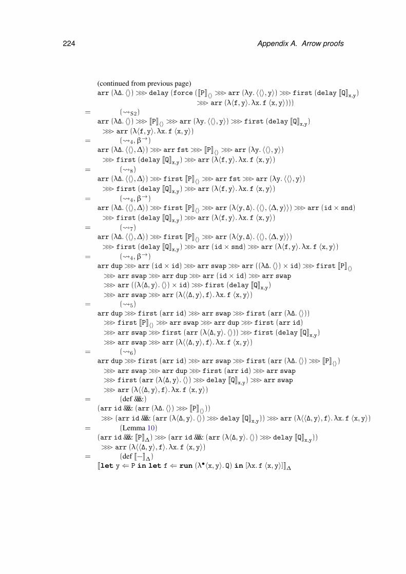
224 Appendix A. Arrow proofs
(continued from previous page)arr (λ∆. 〈〉)>>> delay (force (JPK〈〉 >>> arr (λy. 〈〈〉, y〉)>>> first (delay JQKx,y)
>>> arr (λ〈f, y〉. λx. f 〈x, y〉)))= ( S2)
arr (λ∆. 〈〉)>>> JPK〈〉 >>> arr (λy. 〈〈〉, y〉)>>> first (delay JQKx,y)
>>> arr (λ〈f, y〉. λx. f 〈x, y〉)= ( 4,β→)
arr (λ∆. 〈〈〉,∆〉)>>> arr fst>>> JPK〈〉 >>> arr (λy. 〈〈〉, y〉)>>> first (delay JQKx,y)>>> arr (λ〈f, y〉. λx. f 〈x, y〉)
= ( 8)arr (λ∆. 〈〈〉,∆〉)>>> first JPK〈〉 >>> arr fst>>> arr (λy. 〈〈〉, y〉)>>> first (delay JQKx,y)>>> arr (λ〈f, y〉. λx. f 〈x, y〉)
= ( 4,β→)arr (λ∆. 〈〈〉,∆〉)>>> first JPK〈〉 >>> arr (λ〈y, ∆〉. 〈〈〉, 〈∆, y〉〉)>>> arr (id× snd)
>>> first (delay JQKx,y)>>> arr (λ〈f, y〉. λx. f 〈x, y〉)= ( 7)
arr (λ∆. 〈〈〉,∆〉)>>> first JPK〈〉 >>> arr (λ〈y, ∆〉. 〈〈〉, 〈∆, y〉〉)>>> first (delay JQKx,y)>>> arr (id× snd)>>> arr (λ〈f, y〉. λx. f 〈x, y〉)
= ( 4,β→)arr dup>>> arr (id× id)>>> arr swap>>> arr ((λ∆. 〈〉)× id)>>> first JPK〈〉>>> arr swap>>> arr dup>>> arr (id× id)>>> arr swap
>>> arr ((λ〈∆, y〉. 〈〉)× id)>>> first (delay JQKx,y)
>>> arr swap>>> arr (λ〈〈∆, y〉, f〉. λx. f 〈x, y〉)= ( 5)
arr dup>>> first (arr id)>>> arr swap>>> first (arr (λ∆. 〈〉))>>> first JPK〈〉 >>> arr swap>>> arr dup>>> first (arr id)
>>> arr swap>>> first (arr (λ〈∆, y〉. 〈〉))>>> first (delay JQKx,y)
>>> arr swap>>> arr (λ〈〈∆, y〉, f〉. λx. f 〈x, y〉)= ( 6)
arr dup>>> first (arr id)>>> arr swap>>> first (arr (λ∆. 〈〉)>>> JPK〈〉)>>> arr swap>>> arr dup>>> first (arr id)>>> arr swap
>>> first (arr (λ〈∆, y〉. 〈〉)>>> delay JQKx,y)>>> arr swap
>>> arr (λ〈〈∆, y〉, f〉. λx. f 〈x, y〉)= (def &&&)
(arr id &&& (arr (λ∆. 〈〉)>>> JPK〈〉))>>> (arr id &&& (arr (λ〈∆, y〉. 〈〉)>>> delay JQKx,y))>>> arr (λ〈〈∆, y〉, f〉. λx. f 〈x, y〉)
= (Lemma 10)(arr id &&& JPK∆)>>> (arr id &&& (arr (λ〈∆, y〉. 〈〉)>>> delay JQKx,y))
>>> arr (λ〈〈∆, y〉, f〉. λx. f 〈x, y〉)= (def J−K∆)
Jlet y⇐ P in let f⇐ run (λ•〈x, y〉. Q) in [λx. f 〈x, y〉]K∆
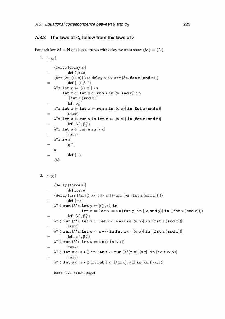
A.3. Equational correspondence between S and CS 225
A.3.3 The laws of CS follow from the laws of S
For each lawM = N of classic arrows with delay we must show 〈[M]〉 = 〈[N]〉.
1. ( S1)
〈[force (delay a)]〉= (def force)〈[arr (λx. 〈〈〉, x〉)>>> delay a>>> arr (λz.fst z (snd z))]〉
= (def 〈[−]〉,β )λ•x.let y⇐ [〈〈〉, x〉] in
let z⇐ let w⇐ run a in [〈w,snd y〉] in[fst z (snd z)]
= (left,β×2 )λ•x.let z⇐ let w⇐ run a in [〈w, x〉] in [fst z (snd z)]
= (assoc)λ•x.let w⇐ run a in let z⇐ [〈w, x〉] in [fst z (snd z)]
= (left,β×1 ,β×2 )λ•x.let w⇐ run a in [w x]
= (run1)λ•x. a • x
= (η )a
= (def 〈[−]〉)〈[a]〉
2. ( S2)
〈[delay (force a)]〉= (def force)〈[delay (arr (λx. 〈〈〉, x〉)>>> a>>> arr (λz. (fst z (snd z))))]〉
= (def 〈[−]〉)λ•〈〉.run (λ•x.let y⇐ [〈〈〉, x〉] in
let z⇐ let w⇐ a • (fst y) in [〈w,snd y〉] in [(fst z (snd z))])
= (left,β×1 ,β×2 )λ•〈〉.run (λ•x.let z⇐ let w⇐ a • 〈〉 in [〈w, x〉] in [(fst z (snd z))])
= (assoc)λ•〈〉.run (λ•x.let w⇐ a • 〈〉 in let z⇐ [〈w, x〉] in [(fst z (snd z))])
= (left,β×1 ,β×2 )λ•〈〉.run (λ•x.let w⇐ a • 〈〉 in [w x])
= (run3)λ•〈〉.let w⇐ a • 〈〉 in let f⇐ run (λ•〈x, w〉. [w x]) in [λx. f 〈x, w〉]
= (run2)λ•〈〉.let w⇐ a • 〈〉 in let f⇐ [λ〈x, w〉. w x] in [λx. f 〈x, w〉]
(continued on next page)
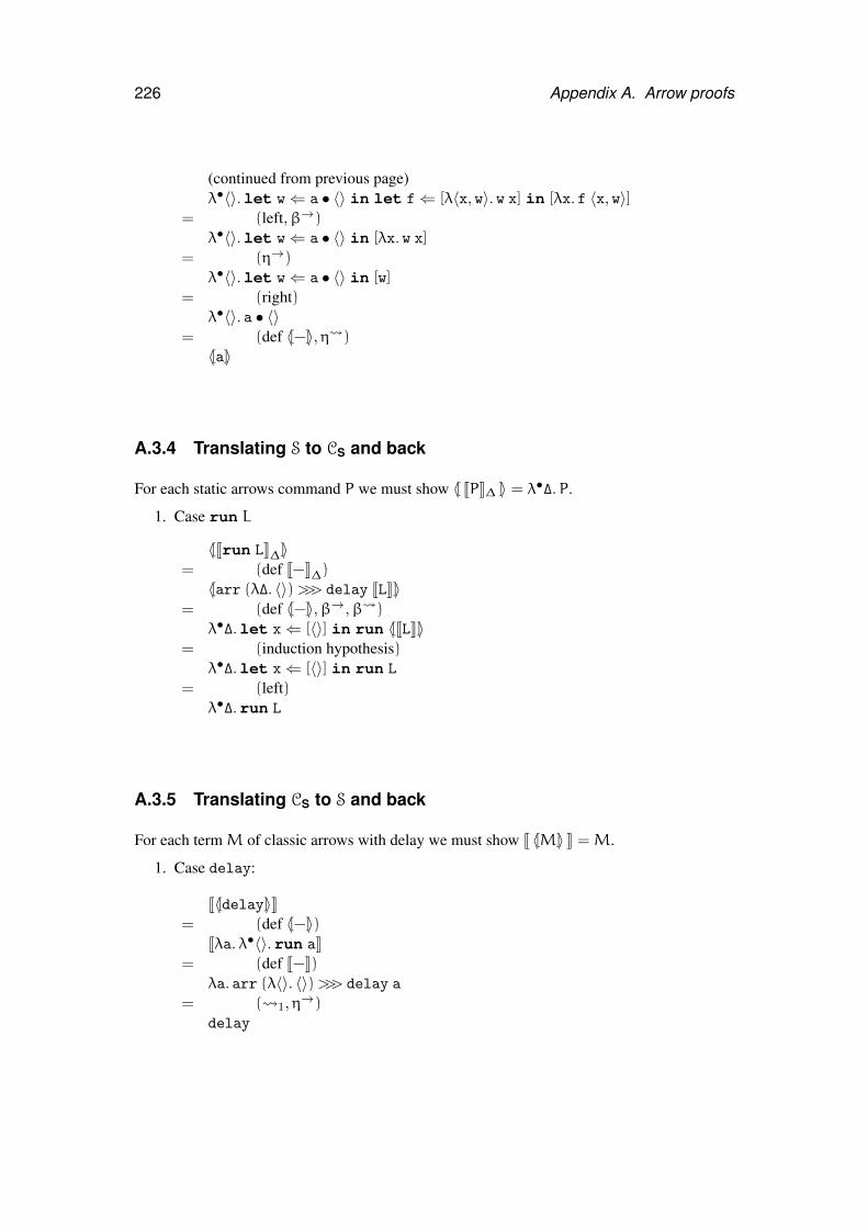
226 Appendix A. Arrow proofs
(continued from previous page)λ•〈〉.let w⇐ a • 〈〉 in let f⇐ [λ〈x, w〉. w x] in [λx. f 〈x, w〉]
= (left,β→)λ•〈〉.let w⇐ a • 〈〉 in [λx. w x]
= (η→)λ•〈〉.let w⇐ a • 〈〉 in [w]
= (right)λ•〈〉. a • 〈〉
= (def 〈[−]〉,η )〈[a]〉
A.3.4 Translating S to CS and back
For each static arrows command P we must show 〈[ JPK∆ ]〉 = λ•∆.P.
1. Case run L
〈[Jrun LK∆]〉= (def J−K∆)〈[arr (λ∆. 〈〉)>>> delay JLK]〉
= (def 〈[−]〉,β→,β )λ•∆.let x⇐ [〈〉] in run 〈[JLK]〉
= (induction hypothesis)λ•∆.let x⇐ [〈〉] in run L
= (left)λ•∆.run L
A.3.5 Translating CS to S and back
For each termM of classic arrows with delay we must show J 〈[M]〉 K =M.
1. Case delay:
J〈[delay]〉K= (def 〈[−]〉)
Jλa. λ•〈〉.run aK= (def J−K)
λa. arr (λ〈〉. 〈〉)>>> delay a
= ( 1,η→)delay
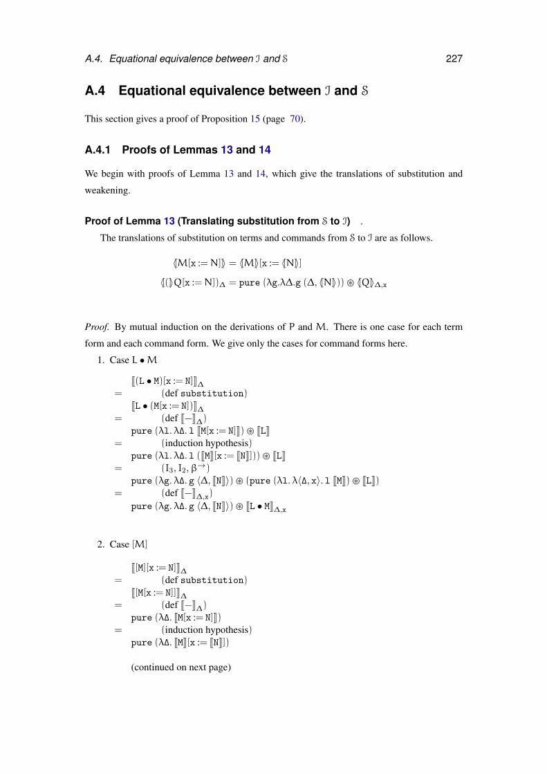
A.4. Equational equivalence between I and S 227
A.4 Equational equivalence between I and S
This section gives a proof of Proposition 15 (page 70).
A.4.1 Proofs of Lemmas 13 and 14
We begin with proofs of Lemma 13 and 14, which give the translations of substitution and
weakening.
Proof of Lemma 13 (Translating substitution from S to I) .
The translations of substitution on terms and commands from S to I are as follows.
〈[M[x :=N]]〉 = 〈[M]〉[x := 〈[N]〉]
〈[(]〉Q[x :=N])∆ = pure (λg.λ∆.g (∆, 〈[N]〉))� 〈[Q]〉∆,x
Proof. By mutual induction on the derivations of P and M. There is one case for each term
form and each command form. We give only the cases for command forms here.
1. Case L •M
J(L • M)[x := N]K∆= (def substitution)
JL • (M[x := N])K∆= (def J−K∆)
pure (λl. λ∆. l JM[x := N]K)� JLK= (induction hypothesis)
pure (λl. λ∆. l (JMK[x := JNK]))� JLK= (I3, I2,β→)
pure (λg. λ∆. g 〈∆, JNK〉)� (pure (λl. λ〈∆, x〉. l JMK)� JLK)= (def J−K∆,x)
pure (λg. λ∆. g 〈∆, JNK〉)� JL • MK∆,x
2. Case [M]
J[M][x := N]K∆= (def substitution)
J[M[x := N]]K∆= (def J−K∆)
pure (λ∆. JM[x := N]K)= (induction hypothesis)
pure (λ∆. JMK[x := JNK])
(continued on next page)
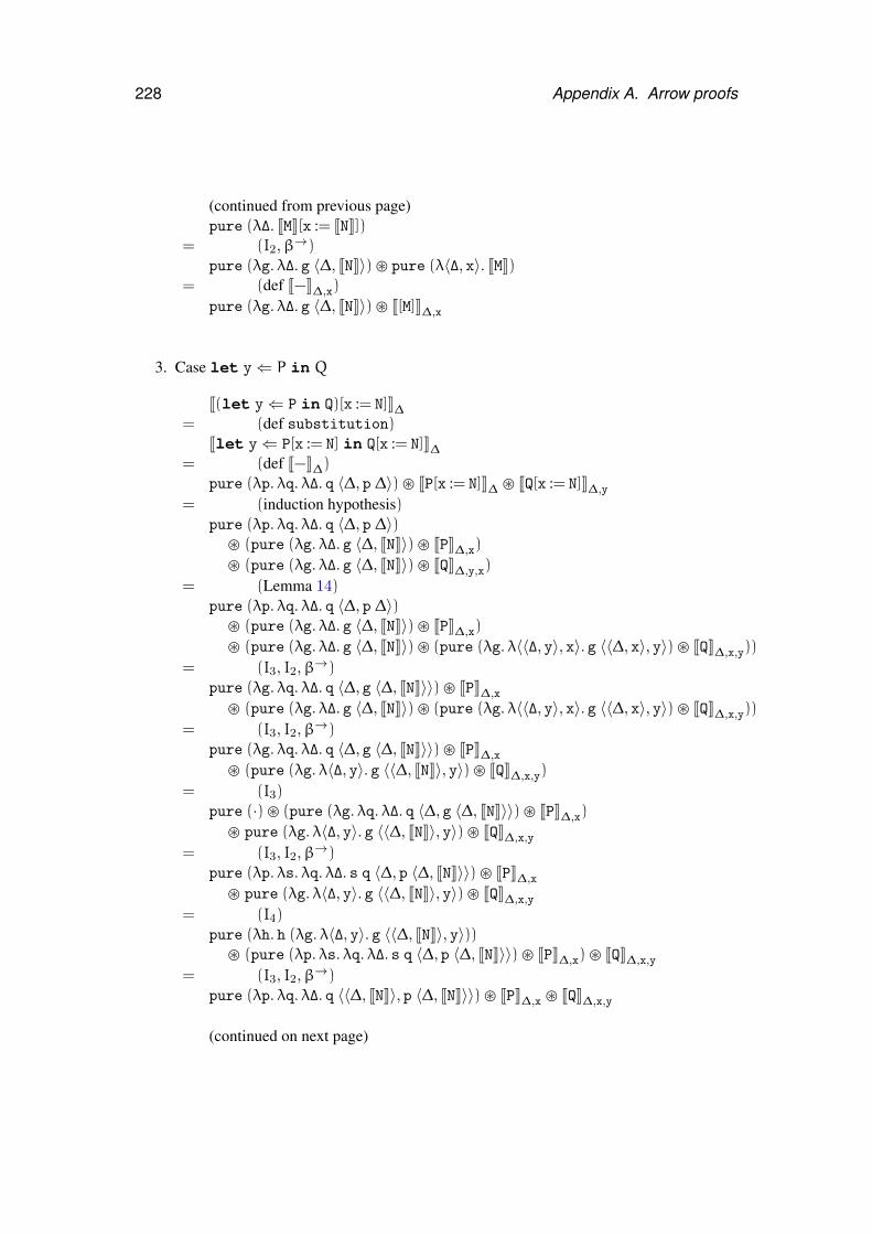
228 Appendix A. Arrow proofs
(continued from previous page)pure (λ∆. JMK[x := JNK])
= (I2,β→)pure (λg. λ∆. g 〈∆, JNK〉)� pure (λ〈∆, x〉. JMK)
= (def J−K∆,x)
pure (λg. λ∆. g 〈∆, JNK〉)� J[M]K∆,x
3. Case let y⇐ P in Q
J(let y⇐ P in Q)[x := N]K∆= (def substitution)
Jlet y⇐ P[x := N] in Q[x := N]K∆= (def J−K∆)
pure (λp. λq. λ∆. q 〈∆, p ∆〉)� JP[x := N]K∆ � JQ[x := N]K∆,y
= (induction hypothesis)pure (λp. λq. λ∆. q 〈∆, p ∆〉)� (pure (λg. λ∆. g 〈∆, JNK〉)� JPK∆,x)
� (pure (λg. λ∆. g 〈∆, JNK〉)� JQK∆,y,x)
= (Lemma 14)pure (λp. λq. λ∆. q 〈∆, p ∆〉)� (pure (λg. λ∆. g 〈∆, JNK〉)� JPK∆,x)
� (pure (λg. λ∆. g 〈∆, JNK〉)� (pure (λg. λ〈〈∆, y〉, x〉. g 〈〈∆, x〉, y〉)� JQK∆,x,y))
= (I3, I2,β→)pure (λg. λq. λ∆. q 〈∆, g 〈∆, JNK〉〉)� JPK∆,x
� (pure (λg. λ∆. g 〈∆, JNK〉)� (pure (λg. λ〈〈∆, y〉, x〉. g 〈〈∆, x〉, y〉)� JQK∆,x,y))
= (I3, I2,β→)pure (λg. λq. λ∆. q 〈∆, g 〈∆, JNK〉〉)� JPK∆,x
� (pure (λg. λ〈∆, y〉. g 〈〈∆, JNK〉, y〉)� JQK∆,x,y)
= (I3)pure (·)� (pure (λg. λq. λ∆. q 〈∆, g 〈∆, JNK〉〉)� JPK∆,x)
� pure (λg. λ〈∆, y〉. g 〈〈∆, JNK〉, y〉)� JQK∆,x,y
= (I3, I2,β→)pure (λp. λs. λq. λ∆. s q 〈∆, p 〈∆, JNK〉〉)� JPK∆,x
� pure (λg. λ〈∆, y〉. g 〈〈∆, JNK〉, y〉)� JQK∆,x,y
= (I4)pure (λh. h (λg. λ〈∆, y〉. g 〈〈∆, JNK〉, y〉))� (pure (λp. λs. λq. λ∆. s q 〈∆, p 〈∆, JNK〉〉)� JPK∆,x)� JQK∆,x,y
= (I3, I2,β→)pure (λp. λq. λ∆. q 〈〈∆, JNK〉, p 〈∆, JNK〉〉)� JPK∆,x � JQK∆,x,y
(continued on next page)
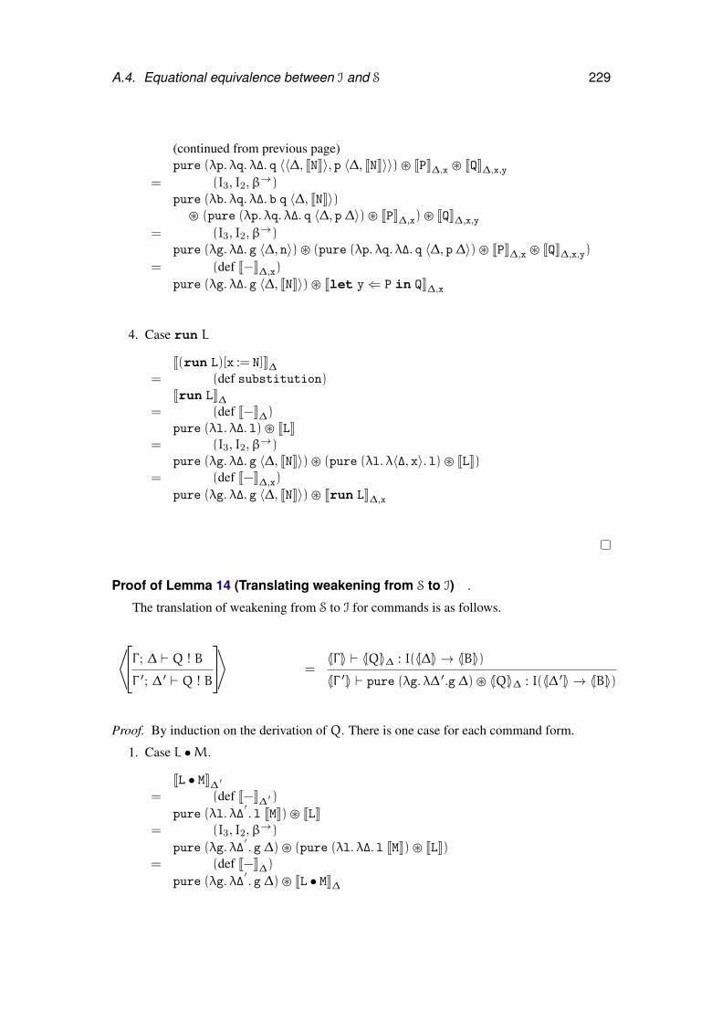
A.4. Equational equivalence between I and S 229
(continued from previous page)pure (λp. λq. λ∆. q 〈〈∆, JNK〉, p 〈∆, JNK〉〉)� JPK∆,x � JQK∆,x,y
= (I3, I2,β→)pure (λb. λq. λ∆. b q 〈∆, JNK〉)� (pure (λp. λq. λ∆. q 〈∆, p ∆〉)� JPK∆,x)� JQK∆,x,y
= (I3, I2,β→)pure (λg. λ∆. g 〈∆, n〉)� (pure (λp. λq. λ∆. q 〈∆, p ∆〉)� JPK∆,x � JQK∆,x,y)
= (def J−K∆,x)
pure (λg. λ∆. g 〈∆, JNK〉)� Jlet y⇐ P in QK∆,x
4. Case run L
J(run L)[x := N]K∆= (def substitution)
Jrun LK∆= (def J−K∆)
pure (λl. λ∆. l)� JLK= (I3, I2,β→)
pure (λg. λ∆. g 〈∆, JNK〉)� (pure (λl. λ〈∆, x〉. l)� JLK)= (def J−K∆,x)
pure (λg. λ∆. g 〈∆, JNK〉)� Jrun LK∆,x
Proof of Lemma 14 (Translating weakening from S to I) .
The translation of weakening from S to I for commands is as follows.
⟨Γ ; ∆ ` Q ! B
Γ ′; ∆ ′ ` Q ! B
⟩ =〈[Γ ]〉 ` 〈[Q]〉∆ : I(〈[∆]〉 → 〈[B]〉)〈[Γ ′]〉 ` pure (λg. λ∆ ′.g ∆)� 〈[Q]〉∆ : I(〈[∆ ′]〉 → 〈[B]〉)
Proof. By induction on the derivation of Q. There is one case for each command form.
1. Case L •M.
JL • MK∆ ′= (def J−K∆ ′ )
pure (λl. λ∆′. l JMK)� JLK
= (I3, I2,β→)
pure (λg. λ∆′. g ∆)� (pure (λl. λ∆. l JMK)� JLK)
= (def J−K∆)pure (λg. λ∆
′. g ∆)� JL • MK∆
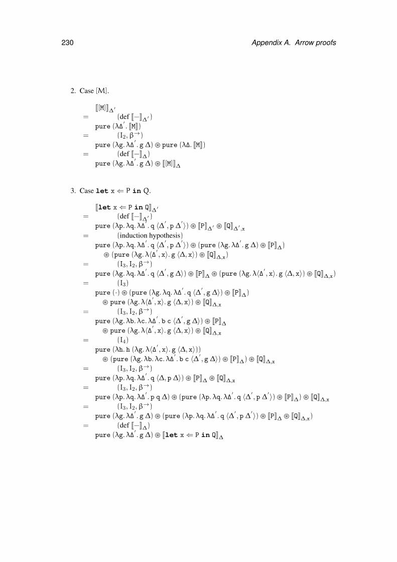
230 Appendix A. Arrow proofs
2. Case [M].
J[M]K∆ ′= (def J−K∆ ′ )
pure (λ∆′. JMK)
= (I2,β→)
pure (λg. λ∆′. g ∆)� pure (λ∆. JMK)
= (def J−K∆)pure (λg. λ∆
′. g ∆)� J[M]K∆
3. Case let x⇐ P in Q.
Jlet x⇐ P in QK∆ ′= (def J−K∆ ′ )
pure (λp. λq. λ∆′. q 〈∆ ′ , p ∆ ′〉)� JPK∆ ′ � JQK∆ ′ ,x
= (induction hypothesis)pure (λp. λq. λ∆
′. q 〈∆ ′ , p ∆ ′〉)� (pure (λg. λ∆
′. g ∆)� JPK∆)
� (pure (λg. λ〈∆ ′ , x〉. g 〈∆, x〉)� JQK∆,x)
= (I3, I2,β→)
pure (λg. λq. λ∆′. q 〈∆ ′ , g ∆〉)� JPK∆ � (pure (λg. λ〈∆ ′ , x〉. g 〈∆, x〉)� JQK∆,x)
= (I3)
pure (·)� (pure (λg. λq. λ∆′. q 〈∆ ′ , g ∆〉)� JPK∆)
� pure (λg. λ〈∆ ′ , x〉. g 〈∆, x〉)� JQK∆,x
= (I3, I2,β→)
pure (λg. λb. λc. λ∆′. b c 〈∆ ′ , g ∆〉)� JPK∆
� pure (λg. λ〈∆ ′ , x〉. g 〈∆, x〉)� JQK∆,x
= (I4)
pure (λh. h (λg. λ〈∆ ′ , x〉. g 〈∆, x〉))� (pure (λg. λb. λc. λ∆
′. b c 〈∆ ′ , g ∆〉)� JPK∆)� JQK∆,x
= (I3, I2,β→)
pure (λp. λq. λ∆′. q 〈∆, p ∆〉)� JPK∆ � JQK∆,x
= (I3, I2,β→)
pure (λp. λq. λ∆′. p q ∆)� (pure (λp. λq. λ∆
′. q 〈∆ ′ , p ∆ ′〉)� JPK∆)� JQK∆,x
= (I3, I2,β→)
pure (λg. λ∆′. g ∆)� (pure (λp. λq. λ∆
′. q 〈∆ ′ , p ∆ ′〉)� JPK∆ � JQK∆,x)
= (def J−K∆)pure (λg. λ∆
′. g ∆)� Jlet x⇐ P in QK∆
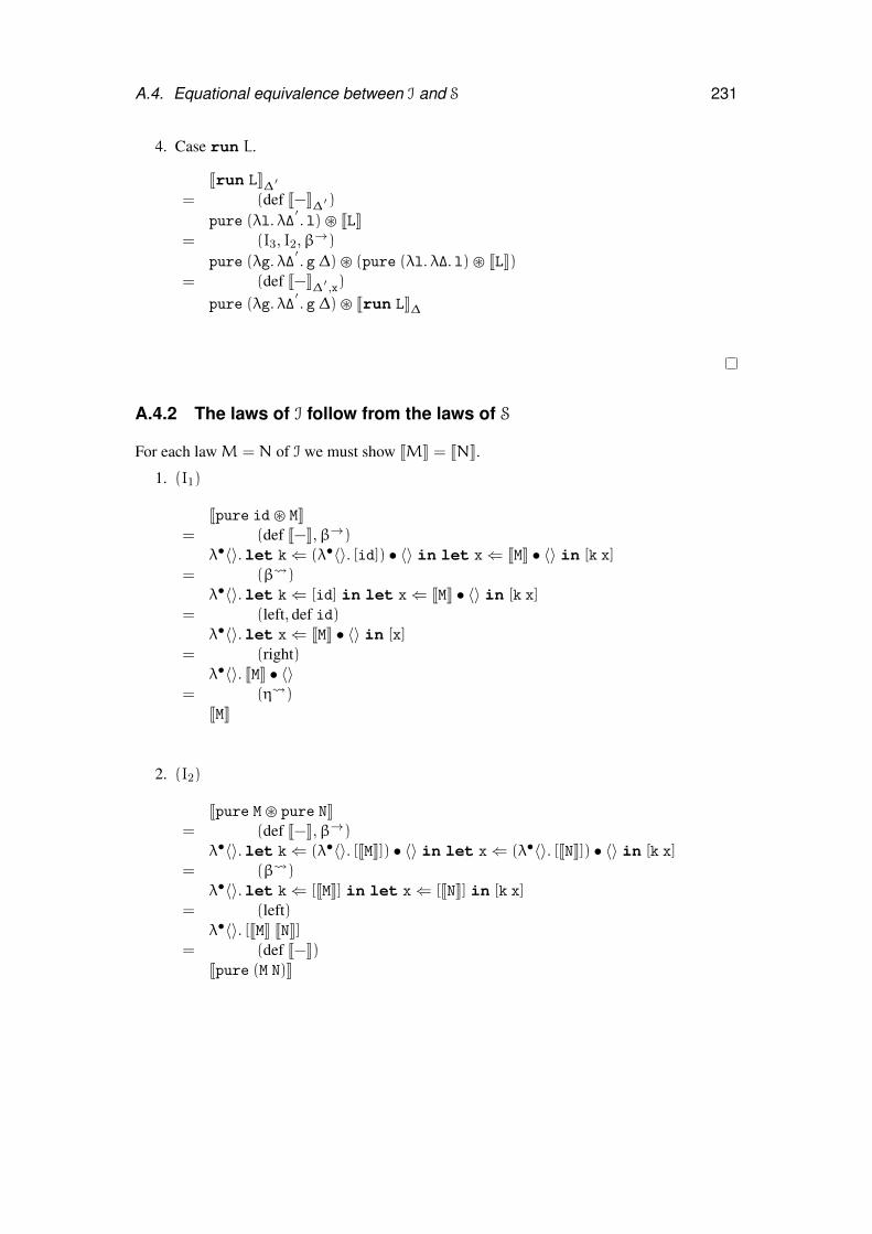
A.4. Equational equivalence between I and S 231
4. Case run L.
Jrun LK∆ ′= (def J−K∆ ′ )
pure (λl. λ∆′. l)� JLK
= (I3, I2,β→)
pure (λg. λ∆′. g ∆)� (pure (λl. λ∆. l)� JLK)
= (def J−K∆ ′ ,x)pure (λg. λ∆
′. g ∆)� Jrun LK∆
A.4.2 The laws of I follow from the laws of S
For each lawM = N of I we must show JMK = JNK.
1. (I1)
Jpure id� MK= (def J−K,β→)
λ•〈〉.let k⇐ (λ•〈〉. [id]) • 〈〉 in let x⇐ JMK • 〈〉 in [k x]= (β )
λ•〈〉.let k⇐ [id] in let x⇐ JMK • 〈〉 in [k x]= (left, def id)
λ•〈〉.let x⇐ JMK • 〈〉 in [x]= (right)
λ•〈〉. JMK • 〈〉= (η )
JMK
2. (I2)
Jpure M� pure NK= (def J−K,β→)
λ•〈〉.let k⇐ (λ•〈〉. [JMK]) • 〈〉 in let x⇐ (λ•〈〉. [JNK]) • 〈〉 in [k x]= (β )
λ•〈〉.let k⇐ [JMK] in let x⇐ [JNK] in [k x]= (left)
λ•〈〉. [JMK JNK]= (def J−K)
Jpure (M N)K
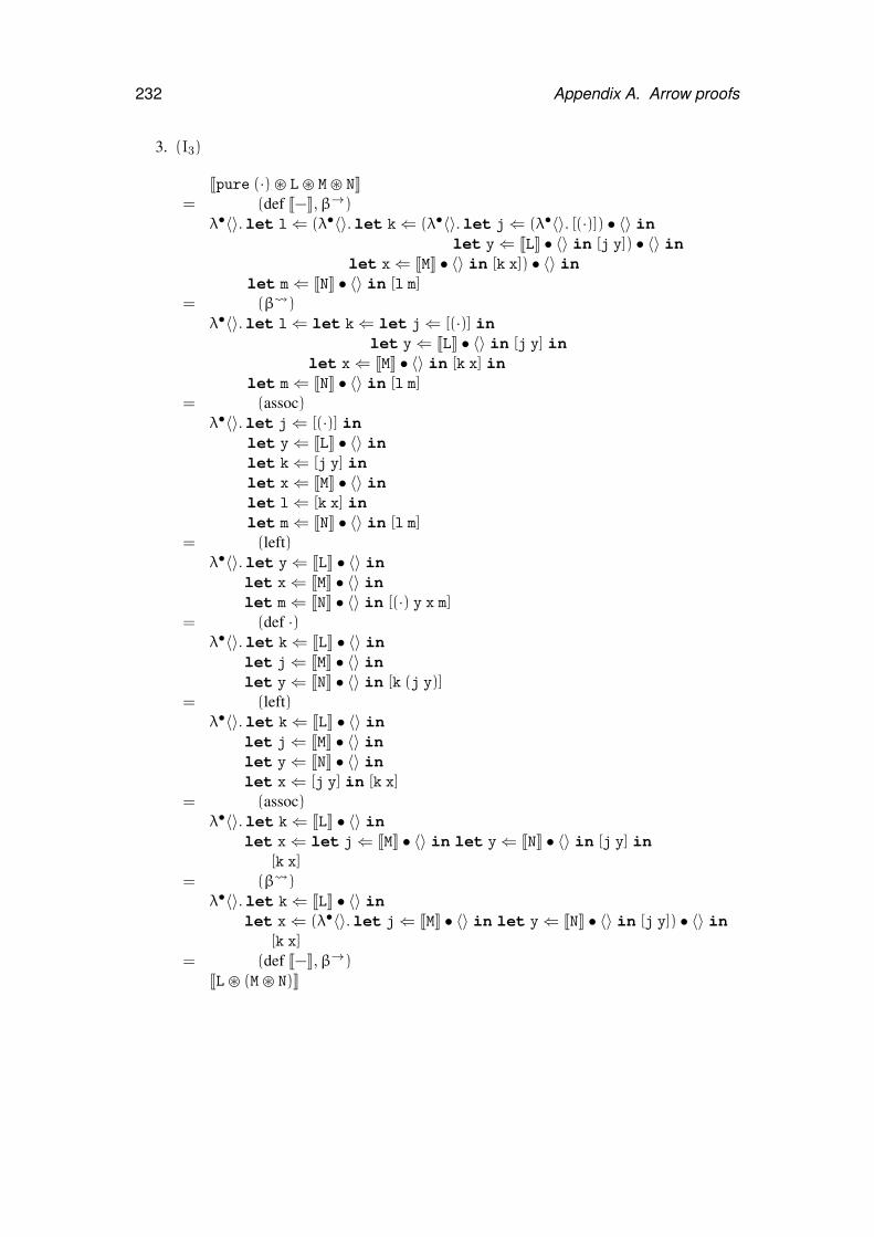
232 Appendix A. Arrow proofs
3. (I3)
Jpure (·)� L� M� NK= (def J−K,β→)
λ•〈〉.let l⇐ (λ•〈〉.let k⇐ (λ•〈〉.let j⇐ (λ•〈〉. [(·)]) • 〈〉 inlet y⇐ JLK • 〈〉 in [j y]) • 〈〉 in
let x⇐ JMK • 〈〉 in [k x]) • 〈〉 inlet m⇐ JNK • 〈〉 in [l m]
= (β )λ•〈〉.let l⇐ let k⇐ let j⇐ [(·)] in
let y⇐ JLK • 〈〉 in [j y] inlet x⇐ JMK • 〈〉 in [k x] in
let m⇐ JNK • 〈〉 in [l m]= (assoc)
λ•〈〉.let j⇐ [(·)] inlet y⇐ JLK • 〈〉 inlet k⇐ [j y] inlet x⇐ JMK • 〈〉 inlet l⇐ [k x] inlet m⇐ JNK • 〈〉 in [l m]
= (left)λ•〈〉.let y⇐ JLK • 〈〉 in
let x⇐ JMK • 〈〉 inlet m⇐ JNK • 〈〉 in [(·) y x m]
= (def ·)λ•〈〉.let k⇐ JLK • 〈〉 in
let j⇐ JMK • 〈〉 inlet y⇐ JNK • 〈〉 in [k (j y)]
= (left)λ•〈〉.let k⇐ JLK • 〈〉 in
let j⇐ JMK • 〈〉 inlet y⇐ JNK • 〈〉 inlet x⇐ [j y] in [k x]
= (assoc)λ•〈〉.let k⇐ JLK • 〈〉 in
let x⇐ let j⇐ JMK • 〈〉 in let y⇐ JNK • 〈〉 in [j y] in[k x]
= (β )λ•〈〉.let k⇐ JLK • 〈〉 in
let x⇐ (λ•〈〉.let j⇐ JMK • 〈〉 in let y⇐ JNK • 〈〉 in [j y]) • 〈〉 in[k x]
= (def J−K,β→)JL� (M� N)K
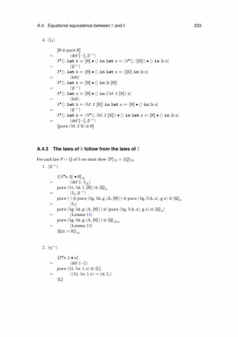
A.4. Equational equivalence between I and S 233
4. (I4)
JM� pure NK= (def J−K,β→)
λ•〈〉.let k⇐ JMK • 〈〉 in let x⇐ (λ•〈〉. [JNK]) • 〈〉 in [k x]= (β )
λ•〈〉.let k⇐ JMK • 〈〉 in let x⇐ [JNK] in [k x]= (left)
λ•〈〉.let k⇐ JMK • 〈〉 in [k JNK]= (β→)
λ•〈〉.let x⇐ JMK • 〈〉 in [(λf. f JNK) x]= (left)
λ•〈〉.let k⇐ [λf. f JNK] in let x⇐ JMK • 〈〉 in [k x]= (β )
λ•〈〉.let k⇐ (λ•〈〉. [λf. f JNK]) • 〈〉 in let x⇐ JMK • 〈〉 in [k x]= (def J−K,β→)
Jpure (λf. f N)� MK
A.4.3 The laws of S follow from the laws of I
For each law P = Q of S we must show 〈[P]〉∆ = 〈[Q]〉∆.
1. (β )
〈[(λ•x. Q) • M]〉∆= (def 〈[−]〉∆)
pure (λl. λ∆. l 〈[M]〉)� 〈[Q]〉x= (I2,β→)
pure (·)� pure (λg. λ∆. g 〈∆, 〈[M]〉〉)� pure (λg. λ〈∆, x〉. g x)� 〈[Q]〉x= (I3)
pure (λg. λ∆. g 〈∆, 〈[M]〉〉)� (pure (λg. λ〈∆, x〉. g x)� 〈[Q]〉x)= (Lemma 14)
pure (λg. λ∆. g 〈∆, 〈[M]〉〉)� 〈[Q]〉∆,x
= (Lemma 13)〈[Q[x := M]]〉∆
2. (η )
〈[λ•x. L • x]〉= (def 〈[−]〉)
pure (λl. λx. l x)� 〈[L]〉= ((λl. λx. l x) = id, I1)〈[L]〉
234 Appendix A. Arrow proofs
3. (left)
〈[let x⇐ [M] in Q]〉∆= (def 〈[−]〉∆)
pure (λp. λq. λ∆. q 〈∆, p ∆〉)� pure (λ∆. 〈[M]〉)� 〈[Q]〉∆,x
= (I2,β→)pure (λq. λ∆. q 〈∆, 〈[M]〉〉)� 〈[Q]〉∆,x
= (Lemma 13)〈[Q[x := M]]〉∆
4. (right)
〈[let x⇐ P in [x]]〉∆= (def 〈[−]〉∆)
pure (λp. λq. λ∆. q 〈∆, p ∆〉)� 〈[P]〉∆ � pure (λ〈∆, x〉. x)= (I4)
pure (λf. f (λ〈∆, x〉. x))� (pure (λp. λq. λ∆. q 〈∆, p ∆〉)� 〈[P]〉∆)= (I3)
pure (·)� pure (λf. f (λ〈∆, x〉. x))� pure (λp. λq. λ∆. q 〈∆, p ∆〉)� 〈[P]〉∆= (I2,β→)
pure (λc. λ∆. c ∆)� 〈[P]〉∆= ((λc. λ∆. c ∆) = id, I1)〈[P]〉∆
5. (assoc)
〈[let y⇐ (let x⇐ P in Q) in R]〉∆= (def 〈[−]〉∆)
pure (λs. λr. λ∆. r 〈∆, s ∆〉)� (pure (λp. λq. λ∆. q 〈∆, p ∆〉)� 〈[P]〉∆ � 〈[Q]〉∆,x)
� 〈[R]〉∆,y
= (I3, I2,β→)pure (λb. λc. λr. λ∆. r 〈∆, (b c) ∆〉)� (pure (λp. λq. λ∆. q 〈∆, p ∆〉)� 〈[P]〉∆)� 〈[Q]〉∆,x � 〈[R]〉∆,y
= (I3, I2,β→)pure (λl. λc. λr. λ∆. r 〈∆, (c 〈∆, l ∆〉)〉)� 〈[P]〉∆ � 〈[Q]〉∆,x � 〈[R]〉∆,y
= (I3, I2,β→)pure (λt. λe. λi. t e (λ〈〈∆, x〉, y〉. i 〈∆, y〉))� (pure (λc. λg. λl. λ∆. l 〈〈∆, c ∆〉, g 〈∆, c ∆〉〉)� 〈[P]〉∆)� 〈[Q]〉∆,x � 〈[R]〉∆,y
= (I3, I2,β→)pure (λb. λe. b e (λg. λ〈〈∆, x〉, y〉. g 〈∆, y〉))� (pure ((·) (·))� (pure (λc. λg. λl. λ∆. l 〈〈∆, c ∆〉, g 〈∆, c ∆〉〉)� 〈[P]〉∆))� 〈[Q]〉∆,x � 〈[R]〉∆,y
(continued on next page)
A.4. Equational equivalence between I and S 235
(continued from previous page)pure (λb. λe. b e (λg. λ〈〈∆, x〉, y〉. g 〈∆, y〉))� (pure ((·) (·))� (pure (λc. λg. λl. λ∆. l 〈〈∆, c ∆〉, g 〈∆, c ∆〉〉)� 〈[P]〉∆))� 〈[Q]〉∆,x � 〈[R]〉∆,y
= (I3, I2,β→)pure (λh. h (λg. λ〈〈∆, x〉, y〉. g 〈∆, y〉))� (pure ((·) (·))� (pure (λc. λg. λl. λ∆. l 〈〈∆, c ∆〉, g 〈∆, c ∆〉〉)� 〈[P]〉∆)
� 〈[Q]〉∆,x)
� 〈[R]〉∆,y
= (I4)pure ((·) (·))� (pure (λc. λg. λl. λ∆. l 〈〈∆, c ∆〉, g 〈∆, c ∆〉〉)� 〈[P]〉∆)� 〈[Q]〉∆,x � pure (λg. λ〈〈∆, x〉, y〉. g 〈∆, y〉)� 〈[R]〉∆,y
= (I3, I2,β→)pure (·)� (pure (λc. λg. λl. λ∆. l 〈〈∆, c ∆〉, g 〈∆, c ∆〉〉)� 〈[P]〉∆ � 〈[Q]〉∆,x)
� pure (λg. λ〈〈∆, x〉, y〉. g 〈∆, y〉)� 〈[R]〉∆,y
= (I3)pure (λc. λg. λl. λ∆. l 〈〈∆, c ∆〉, g 〈∆, c ∆〉〉)� 〈[P]〉∆ � 〈[Q]〉∆,x
� (pure (λg. λ〈〈∆, x〉, y〉. g 〈∆, y〉)� 〈[R]〉∆,y)
= (I3, I2,β→)pure (λf. f (λq. λr. λ∆. r 〈∆, q ∆〉))� (pure (λe. λf. λg. λl. λ∆. f g l 〈∆, e ∆〉)� 〈[P]〉∆)� 〈[Q]〉∆,x � (pure (λg. λ〈〈∆, x〉, y〉. g 〈∆, y〉)� 〈[R]〉∆,y)
= (I4)pure (λe. λf. λg. λl. λ∆. f g l 〈∆, e ∆〉)� 〈[P]〉∆� pure (λq. λr. λ∆. r 〈∆, q ∆〉)� 〈[Q]〉∆,x � (pure (λg. λ〈〈∆, x〉, y〉. g 〈∆, y〉)� 〈[R]〉∆,y)
= (I3, I2,β→)pure (·)� (pure (λc. λk. λl. λ∆. k l 〈∆, c ∆〉)� 〈[P]〉∆)� pure (λq. λr. λ∆. r 〈∆, q ∆〉)� 〈[Q]〉∆,x � (pure (λg. λ〈〈∆, x〉, y〉. g 〈∆, y〉)� 〈[R]〉∆,y)
= (I3)pure (λc. λk. λl. λ∆. k l 〈∆, c ∆〉)� 〈[P]〉∆� (pure (λq. λr. λ∆. r 〈∆, q ∆〉)� 〈[Q]〉∆,x)
� (pure (λg. λ〈〈∆, x〉, y〉. g 〈∆, y〉)� 〈[R]〉∆,y)
= (I3, I2,β→)pure (·)� (pure (λp. λq. λ∆. q 〈∆, p ∆〉)� 〈[P]〉∆)� (pure (λq. λr. λ∆. r 〈∆, q ∆〉)� 〈[Q]〉∆,x)
� (pure (λg. λ〈〈∆, x〉, y〉. g 〈∆, y〉)� 〈[R]〉∆,y)
(continued on next page)
236 Appendix A. Arrow proofs
(continued from previous page)pure (·)� (pure (λp. λq. λ∆. q 〈∆, p ∆〉)� 〈[P]〉∆)� (pure (λq. λr. λ∆. r 〈∆, q ∆〉)� 〈[Q]〉∆,x)
� (pure (λg. λ〈〈∆, x〉, y〉. g 〈∆, y〉)� 〈[R]〉∆,y)
= (I3)pure (λp. λq. λ∆. q 〈∆, p ∆〉)� 〈[P]〉∆� (pure (λq. λr. λ∆. r 〈∆, q ∆〉)� 〈[Q]〉∆,x
� (pure (λg. λ〈〈∆, x〉, y〉. g 〈∆, y〉)� 〈[R]〉∆,y))
= (Lemma 14)pure (λp. λq. λ∆. q 〈∆, p ∆〉)� 〈[P]〉∆� (pure (λq. λr. λ∆. r 〈∆, q ∆〉)� 〈[Q]〉∆,x � 〈[R]〉∆,x,y)
= (def 〈[−]〉∆)〈[let x⇐ P in let y⇐ Q in R]〉∆
6. (run1)
〈[L • M]〉∆= (def 〈[−]〉∆)
pure (λl. λ∆. l 〈[M]〉)� 〈[L]〉= (I2,β→)
pure (·)� pure (λg. g (λ〈∆, f〉. f 〈[M]〉))� pure (λc. λq. λ∆. q 〈∆, c〉)� 〈[L]〉= (I3)
pure (λg. g (λ〈∆, f〉. f 〈[M]〉))� (pure (λc. λq. λ∆. q 〈∆, c〉)� 〈[L]〉)= (I4)
pure (λc. λq. λ∆. q 〈∆, c〉)� 〈[L]〉� pure (λ〈∆, f〉. f 〈[M]〉)= (I3, I2,β→)
pure (λp. λq. λ∆. q 〈∆, p ∆〉)� (pure (λl. λ∆. l)� 〈[L]〉)� pure (λ〈∆, f〉. f 〈[M]〉)= (def 〈[−]〉∆)〈[let f⇐ run L in [f M]]〉
7. (run2)
〈[run (λ•x. [M])]〉∆= (def 〈[−]〉∆)
pure (λl. λ∆. l)� pure (λx. 〈[M]〉)= (I2)
pure (λ∆. λx. M)= (def 〈[−]〉∆)〈[[λx. M]]〉∆
A.4. Equational equivalence between I and S 237
8. (run3)
〈[run (λ•x.let y⇐ P in Q)]〉∆= (def 〈[−]〉∆)
pure const� (pure (λp. λq. λx. q 〈x, p x〉)� 〈[P]〉x � 〈[Q]〉x,y)
= (Lemma 14)pure const� (pure (λp. λq. λx. q 〈x, p x〉)� (pure (λg. λx. g 〈〉)� 〈[P]〉〈〉)� 〈[Q]〉x,y)
= (I3, I2,β→)pure const� (pure (λg. (λq. λx. q 〈x, g 〈〉〉))� 〈[P]〉〈〉 � 〈[Q]〉x,y)
= (I3, I2)pure (λh. const · h)� (pure (λg. (λq. λx. q 〈x, g 〈〉〉))� 〈[P]〉〈〉)� 〈[Q]〉x,y
= (I3, I2,β→)pure (λp. λq. λd. λx. q 〈x, p 〈〉〉)� 〈[P]〉〈〉 � 〈[Q]〉x,y
= (I3, I2)pure ((·) const)� (pure (λp. λq. λx. q 〈x, p 〈〉〉)� 〈[P]〉〈〉)� 〈[Q]〉x,y
= (I3, I2,β→)pure (λp. λq. λz. λx. q 〈x, p 〈〉〉)� 〈[P]〉〈〉 � 〈[Q]〉x,y
= (I3, I2,β→)pure (λh. h (λf. λ〈∆, y〉. λx. f 〈x, y〉))� (pure (λp. λb. λq. λz. b q 〈z, p 〈〉〉)� 〈[P]〉〈〉)� 〈[Q]〉x,y
= (I4)pure (λp. λb. λq. λz. b q 〈z, p 〈〉〉)� 〈[P]〉〈〉� pure (λf. λ〈∆, y〉. λx. f 〈x, y〉)� 〈[Q]〉x,y
= (I3, I2,β→)pure (λp. (λq. λz. q 〈z, p 〈〉〉))� 〈[P]〉〈〉� (pure (λh. h (λ〈〈∆, y〉, f〉. λx. f 〈x, y〉))� (pure (λn. λs. λ〈∆, y〉. s 〈〈∆, y〉, n〉)� 〈[Q]〉x,y))
= (I4)pure (λp. (λq. λ∆. q 〈∆, p 〈〉〉))� 〈[P]〉〈〉� (pure (λn. λs. λ〈∆, y〉. s 〈〈∆, y〉, n〉)� 〈[Q]〉x,y
� pure (λ〈〈∆, y〉, f〉. λx. f 〈x, y〉))= (I3, I2,β→)
pure (λp. λq. λ∆. q 〈∆, p ∆〉)� (pure (λg. λ∆. g 〈〉)� 〈[P]〉〈〉)� (pure (λr. λs. λ〈∆, y〉. s 〈〈∆, y〉, r 〈∆, y〉〉)� (pure const� 〈[Q]〉x,y)
� pure (λ〈〈∆, y〉, f〉. λx. f 〈x, y〉))= (Lemma 14)
pure (λp. λq. λ∆. q 〈∆, p ∆〉)� 〈[P]〉∆� (pure (λr. λs. λ〈∆, y〉. s 〈〈∆, y〉, r 〈∆, y〉〉)� (pure const� 〈[Q]〉x,y)
� pure (λ〈〈∆, y〉, f〉. λx. f 〈x, y〉))= (def 〈[−]〉∆)〈[let y⇐ P in let f⇐ run (λ•〈x, y〉. Q) in [λx. f 〈x, y〉]]〉∆
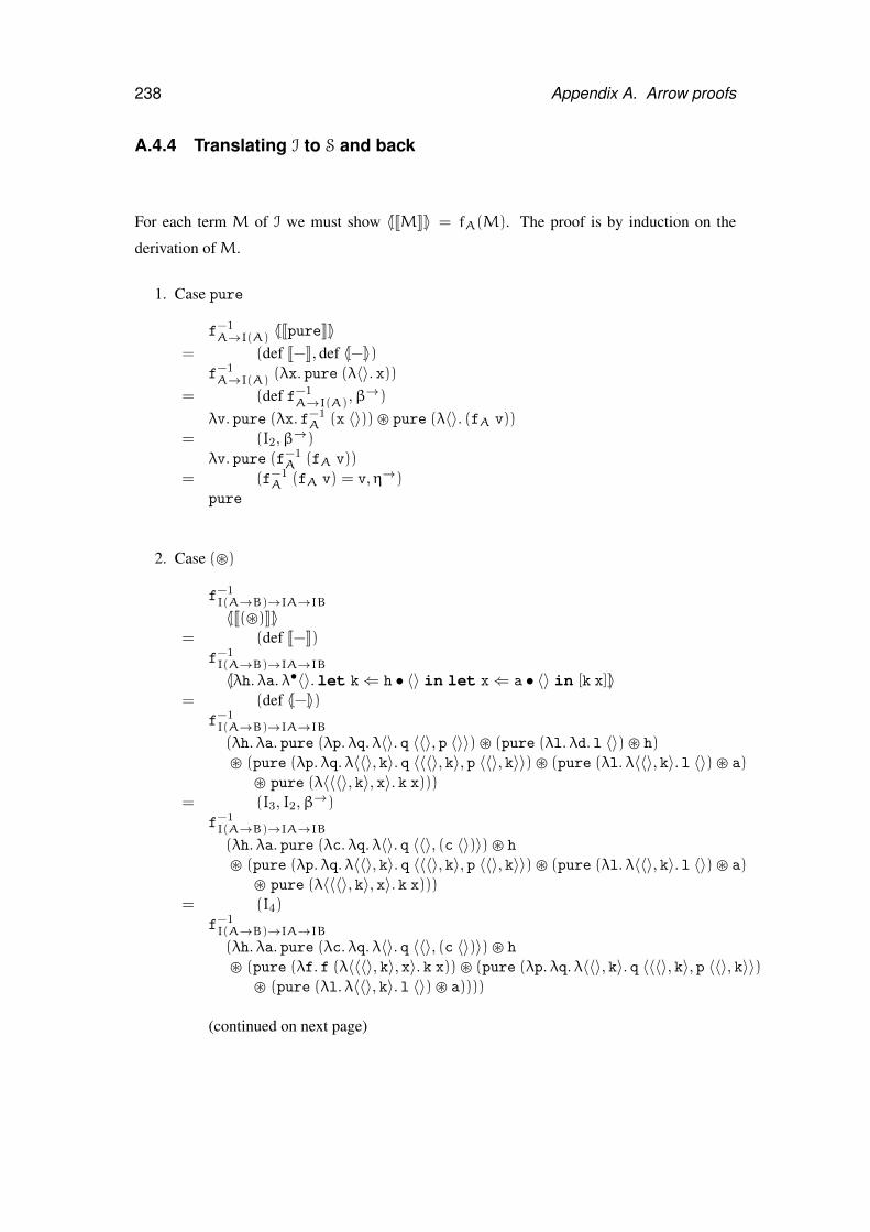
238 Appendix A. Arrow proofs
A.4.4 Translating I to S and back
For each term M of I we must show 〈[JMK]〉 = fA(M). The proof is by induction on the
derivation ofM.
1. Case pure
f−1A→I(A) 〈[JpureK]〉
= (def J−K, def 〈[−]〉)f−1A→I(A) (λx. pure (λ〈〉. x))
= (def f−1A→I(A),β
→)
λv. pure (λx. f−1A (x 〈〉))� pure (λ〈〉. (fA v))
= (I2,β→)
λv. pure (f−1A (fA v))
= (f−1A (fA v) = v,η→)
pure
2. Case (�)
f−1I(A→B)→IA→IB〈[J(�)K]〉
= (def J−K)f−1I(A→B)→IA→IB〈[λh. λa. λ•〈〉.let k⇐ h • 〈〉 in let x⇐ a • 〈〉 in [k x]]〉
= (def 〈[−]〉)f−1I(A→B)→IA→IB(λh. λa. pure (λp. λq. λ〈〉. q 〈〈〉, p 〈〉〉)� (pure (λl. λd. l 〈〉)� h)� (pure (λp. λq. λ〈〈〉, k〉. q 〈〈〈〉, k〉, p 〈〈〉, k〉〉)� (pure (λl. λ〈〈〉, k〉. l 〈〉)� a)
� pure (λ〈〈〈〉, k〉, x〉. k x)))= (I3, I2,β→)
f−1I(A→B)→IA→IB(λh. λa. pure (λc. λq. λ〈〉. q 〈〈〉, (c 〈〉)〉)� h
� (pure (λp. λq. λ〈〈〉, k〉. q 〈〈〈〉, k〉, p 〈〈〉, k〉〉)� (pure (λl. λ〈〈〉, k〉. l 〈〉)� a)� pure (λ〈〈〈〉, k〉, x〉. k x)))
= (I4)
f−1I(A→B)→IA→IB(λh. λa. pure (λc. λq. λ〈〉. q 〈〈〉, (c 〈〉)〉)� h
� (pure (λf. f (λ〈〈〈〉, k〉, x〉. k x))� (pure (λp. λq. λ〈〈〉, k〉. q 〈〈〈〉, k〉, p 〈〈〉, k〉〉)� (pure (λl. λ〈〈〉, k〉. l 〈〉)� a))))
(continued on next page)
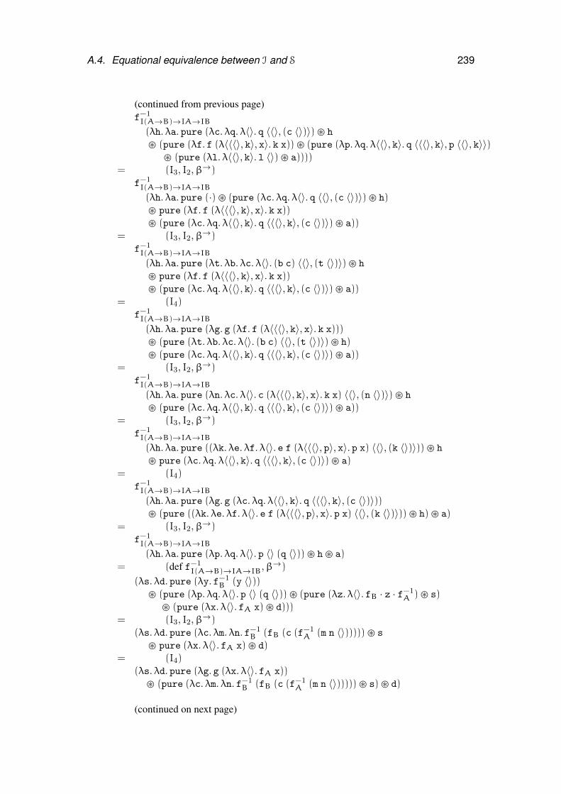
A.4. Equational equivalence between I and S 239
(continued from previous page)f−1I(A→B)→IA→IB(λh. λa. pure (λc. λq. λ〈〉. q 〈〈〉, (c 〈〉)〉)� h
� (pure (λf. f (λ〈〈〈〉, k〉, x〉. k x))� (pure (λp. λq. λ〈〈〉, k〉. q 〈〈〈〉, k〉, p 〈〈〉, k〉〉)� (pure (λl. λ〈〈〉, k〉. l 〈〉)� a))))
= (I3, I2,β→)
f−1I(A→B)→IA→IB(λh. λa. pure (·)� (pure (λc. λq. λ〈〉. q 〈〈〉, (c 〈〉)〉)� h)� pure (λf. f (λ〈〈〈〉, k〉, x〉. k x))� (pure (λc. λq. λ〈〈〉, k〉. q 〈〈〈〉, k〉, (c 〈〉)〉)� a))
= (I3, I2,β→)
f−1I(A→B)→IA→IB(λh. λa. pure (λt. λb. λc. λ〈〉. (b c) 〈〈〉, (t 〈〉)〉)� h
� pure (λf. f (λ〈〈〈〉, k〉, x〉. k x))� (pure (λc. λq. λ〈〈〉, k〉. q 〈〈〈〉, k〉, (c 〈〉)〉)� a))
= (I4)
f−1I(A→B)→IA→IB(λh. λa. pure (λg. g (λf. f (λ〈〈〈〉, k〉, x〉. k x)))� (pure (λt. λb. λc. λ〈〉. (b c) 〈〈〉, (t 〈〉)〉)� h)� (pure (λc. λq. λ〈〈〉, k〉. q 〈〈〈〉, k〉, (c 〈〉)〉)� a))
= (I3, I2,β→)
f−1I(A→B)→IA→IB(λh. λa. pure (λn. λc. λ〈〉. c (λ〈〈〈〉, k〉, x〉. k x) 〈〈〉, (n 〈〉)〉)� h
� (pure (λc. λq. λ〈〈〉, k〉. q 〈〈〈〉, k〉, (c 〈〉)〉)� a))= (I3, I2,β→)
f−1I(A→B)→IA→IB(λh. λa. pure ((λk. λe. λf. λ〈〉. e f (λ〈〈〈〉, p〉, x〉. p x) 〈〈〉, (k 〈〉)〉))� h
� pure (λc. λq. λ〈〈〉, k〉. q 〈〈〈〉, k〉, (c 〈〉)〉)� a)= (I4)
f−1I(A→B)→IA→IB(λh. λa. pure (λg. g (λc. λq. λ〈〈〉, k〉. q 〈〈〈〉, k〉, (c 〈〉)〉))� (pure ((λk. λe. λf. λ〈〉. e f (λ〈〈〈〉, p〉, x〉. p x) 〈〈〉, (k 〈〉)〉))� h)� a)
= (I3, I2,β→)
f−1I(A→B)→IA→IB(λh. λa. pure (λp. λq. λ〈〉. p 〈〉 (q 〈〉))� h� a)
= (def f−1I(A→B)→IA→IB,β→)
(λs. λd. pure (λy. f−1B (y 〈〉))
� (pure (λp. λq. λ〈〉. p 〈〉 (q 〈〉))� (pure (λz. λ〈〉. fB · z · f−1A )� s)
� (pure (λx. λ〈〉. fA x)� d)))= (I3, I2,β→)
(λs. λd. pure (λc. λm. λn. f−1B (fB (c (f−1
A (m n 〈〉)))))� s
� pure (λx. λ〈〉. fA x)� d)= (I4)
(λs. λd. pure (λg. g (λx. λ〈〉. fA x))
� (pure (λc. λm. λn. f−1B (fB (c (f−1
A (m n 〈〉)))))� s)� d)
(continued on next page)
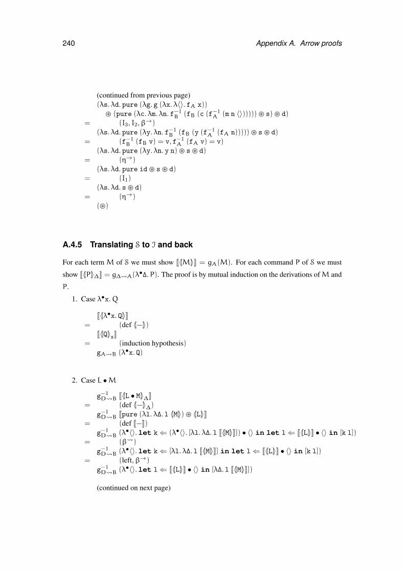
240 Appendix A. Arrow proofs
(continued from previous page)(λs. λd. pure (λg. g (λx. λ〈〉. fA x))
� (pure (λc. λm. λn. f−1B (fB (c (f−1
A (m n 〈〉)))))� s)� d)= (I3, I2,β→)
(λs. λd. pure (λy. λn. f−1B (fB (y (f−1
A (fA n)))))� s� d)
= (f−1B (fB v) = v, f−1
A (fA v) = v)(λs. λd. pure (λy. λn. y n)� s� d)
= (η→)(λs. λd. pure id� s� d)
= (I1)(λs. λd. s� d)
= (η→)(�)
A.4.5 Translating S to I and back
For each term M of S we must show J〈[M]〉K = gA(M). For each command P of S we must
show J〈[P]〉∆K = g∆ A(λ•∆.P). The proof is by mutual induction on the derivations ofM and
P.
1. Case λ•x.Q
J〈[λ•x. Q]〉K= (def 〈[−]〉)
J〈[Q]〉xK= (induction hypothesis)
gA B (λ•x. Q)
2. Case L •M
g−1D B J〈[L • M]〉∆K
= (def 〈[−]〉∆)g−1D B Jpure (λl. λ∆. l 〈[M]〉)� 〈[L]〉K
= (def J−K)g−1D B (λ•〈〉.let k⇐ (λ•〈〉. [λl. λ∆. l J〈[M]〉K]) • 〈〉 in let l⇐ J〈[L]〉K • 〈〉 in [k l])
= (β )
g−1D B (λ•〈〉.let k⇐ [λl. λ∆. l J〈[M]〉K] in let l⇐ J〈[L]〉K • 〈〉 in [k l])
= (left,β→)
g−1D B (λ•〈〉.let l⇐ J〈[L]〉K • 〈〉 in [λ∆. l J〈[M]〉K])
(continued on next page)
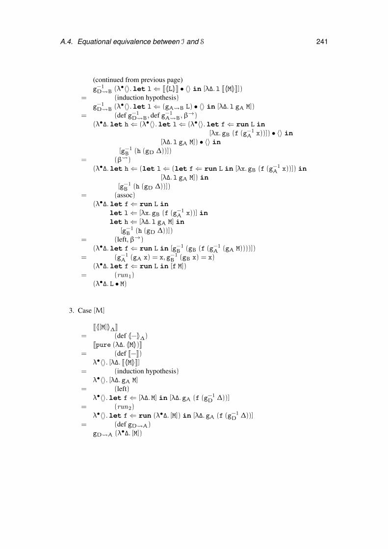
A.4. Equational equivalence between I and S 241
(continued from previous page)g−1D B (λ•〈〉.let l⇐ J〈[L]〉K • 〈〉 in [λ∆. l J〈[M]〉K])
= (induction hypothesis)g−1D B (λ•〈〉.let l⇐ (gA B L) • 〈〉 in [λ∆. l gA M])
= (def g−1D B, def g−1
A B,β→)(λ•∆.let h⇐ (λ•〈〉.let l⇐ (λ•〈〉.let f⇐ run L in
[λx. gB (f (g−1A x))]) • 〈〉 in
[λ∆. l gA M]) • 〈〉 in[g−1B (h (gD ∆))])
= (β )
(λ•∆.let h⇐ (let l⇐ (let f⇐ run L in [λx. gB (f (g−1A x))]) in
[λ∆. l gA M]) in[g−1B (h (gD ∆))])
= (assoc)(λ•∆.let f⇐ run L in
let l⇐ [λx. gB (f (g−1A x))] in
let h⇐ [λ∆. l gA M] in[g−1B (h (gD ∆))])
= (left,β→)
(λ•∆.let f⇐ run L in [g−1B (gB (f (g−1
A (gA M))))])
= (g−1A (gA x) = x, g−1
B (gB x) = x)(λ•∆.let f⇐ run L in [f M])
= (run1)(λ•∆. L • M)
3. Case [M]
J〈[[M]]〉∆K= (def 〈[−]〉∆)
Jpure (λ∆. 〈[M]〉)K= (def J−K)
λ•〈〉. [λ∆. J〈[M]〉K]= (induction hypothesis)
λ•〈〉. [λ∆. gA M]= (left)
λ•〈〉.let f⇐ [λ∆. M] in [λ∆. gA (f (g−1D ∆))]
= (run2)
λ•〈〉.let f⇐ run (λ•∆. [M]) in [λ∆. gA (f (g−1D ∆))]
= (def gD A)gD A (λ•∆. [M])
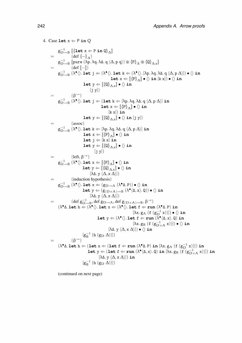
242 Appendix A. Arrow proofs
4. Case let x⇐ P in Q
g−1D B J〈[let x⇐ P in Q]〉∆K
= (def 〈[−]〉∆)g−1D B Jpure (λp. λq. λ∆. q 〈∆, p q〉)� 〈[P]〉∆ � 〈[Q]〉∆,xK
= (def J−K)g−1D B (λ•〈〉.let j⇐ (λ•〈〉.let k⇐ (λ•〈〉. [λp. λq. λ∆. q 〈∆, p ∆〉]) • 〈〉 in
let x⇐ J〈[P]〉∆K • 〈〉 in [k x]) • 〈〉 inlet y⇐ J〈[Q]〉∆,xK • 〈〉 in
[j y])= (β )
g−1D B (λ•〈〉.let j⇐ (let k⇐ [λp. λq. λ∆. q 〈∆, p ∆〉] in
let x⇐ J〈[P]〉∆K • 〈〉 in[k x]) in
let y⇐ J〈[Q]〉∆,xK • 〈〉 in [j y])
= (assoc)g−1D B (λ•〈〉.let k⇐ [λp. λq. λ∆. q 〈∆, p ∆〉] in
let x⇐ J〈[P]〉∆K • 〈〉 inlet j⇐ [k x] inlet y⇐ J〈[Q]〉∆,xK • 〈〉 in
[j y])= (left,β→)
g−1D B (λ•〈〉.let x⇐ J〈[P]〉∆K • 〈〉 in
let y⇐ J〈[Q]〉∆,xK • 〈〉 in[λ∆. y 〈∆, x ∆〉])
= (induction hypothesis)g−1D B (λ•〈〉.let x⇐ (gD A (λ•∆. P)) • 〈〉 in
let y⇐ (g(D×A) B (λ•〈∆, x〉. Q)) • 〈〉 in[λ∆. y 〈∆, x ∆〉])
= (def g−1D B, def gD A, def g(D×A) B,β→)
(λ•∆.let h⇐ (λ•〈〉.let x⇐ (λ•〈〉.let f⇐ run (λ•∆. P) in[λx. gA (f (g−1
D x))]) • 〈〉 inlet y⇐ (λ•〈〉.let f⇐ run (λ•〈∆, x〉. Q) in
[λx. gB (f (g−1D×A x))]) • 〈〉 in
[λ∆. y 〈∆, x ∆〉]) • 〈〉 in[g−1B (h (gD ∆))])
= (β )
(λ•∆.let h⇐ (let x⇐ (let f⇐ run (λ•∆. P) in [λx. gA (f (g−1D x))]) in
let y⇐ (let f⇐ run (λ•〈∆, x〉. Q) in [λx. gB (f (g−1D×A x))]) in
[λ∆. y 〈∆, x ∆〉]) in[g−1B (h (gD ∆))])
(continued on next page)
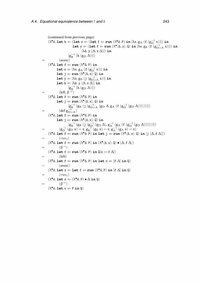
A.4. Equational equivalence between I and S 243
(continued from previous page)(λ•∆.let h⇐ (let x⇐ (let f⇐ run (λ•∆. P) in [λx. gA (f (g−1
D x))]) inlet y⇐ (let f⇐ run (λ•〈∆, x〉. Q) in [λx. gB (f (g−1
D×A x))]) in[λ∆. y 〈∆, x ∆〉]) in
[g−1B (h (gD ∆))])
= (assoc)(λ•∆.let f⇐ run (λ•∆. P) in
let x⇐ [λx. gA (f (g−1D x))] in
let j⇐ run (λ•〈∆, x〉. Q) inlet y⇐ [λx. gB (j (g−1
D×A x))] inlet h⇐ [λ∆. y 〈∆, x ∆〉] in
[g−1B (h (gD ∆))])
= (left,β→)(λ•∆.let f⇐ run (λ•∆. P) in
let j⇐ run (λ•〈∆, x〉. Q) in[g−1B (gB (j (g−1
D×A 〈gD ∆, gA (f (g−1D (gD ∆)))〉)))])
= (def g−1D×A)
(λ•∆.let f⇐ run (λ•∆. P) inlet j⇐ run (λ•〈∆, x〉. Q) in
[g−1B (gB (j 〈g−1
D (gD ∆), g−1A (gA (f (g−1
D (gD ∆))))〉))])= (g−1
D (gD x) = x, g−1B (gB x) = x, g−1
A (gA x) = x)(λ•∆.let f⇐ run (λ•∆. P) in let j⇐ run (λ•〈∆, x〉. Q) in [j 〈∆, f ∆〉])
= (run1)(λ•∆.let f⇐ run (λ•∆. P) in (λ•〈∆, x〉. Q) • 〈∆, f ∆〉)
= (β )(λ•∆.let f⇐ run (λ•∆. P) in Q[x := f ∆])
= (left)(λ•∆.let f⇐ run (λ•∆. P) in let x⇐ [f ∆] in Q)
= (assoc)(λ•∆.let x⇐ let f⇐ run (λ•∆. P) in [f ∆] in Q)
= (run1)(λ•∆.let x⇐ (λ•∆. P) • ∆ in Q)
= (β )(λ•∆.let x⇐ P in Q)
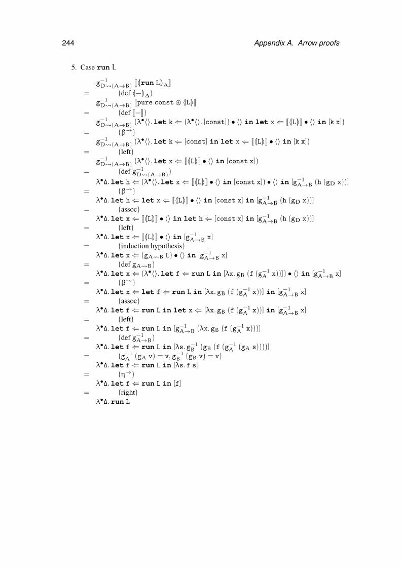
244 Appendix A. Arrow proofs
5. Case run L
g−1D (A→B) J〈[run L]〉∆K
= (def 〈[−]〉∆)g−1D (A→B) Jpure const� 〈[L]〉K
= (def J−K)g−1D (A→B) (λ
•〈〉.let k⇐ (λ•〈〉. [const]) • 〈〉 in let x⇐ J〈[L]〉K • 〈〉 in [k x])
= (β )
g−1D (A→B) (λ
•〈〉.let k⇐ [const] in let x⇐ J〈[L]〉K • 〈〉 in [k x])
= (left)g−1D (A→B) (λ
•〈〉.let x⇐ J〈[L]〉K • 〈〉 in [const x])
= (def g−1D (A→B))
λ•∆.let h⇐ (λ•〈〉.let x⇐ J〈[L]〉K • 〈〉 in [const x]) • 〈〉 in [g−1A→B (h (gD x))]
= (β )
λ•∆.let h⇐ let x⇐ J〈[L]〉K • 〈〉 in [const x] in [g−1A→B (h (gD x))]
= (assoc)λ•∆.let x⇐ J〈[L]〉K • 〈〉 in let h⇐ [const x] in [g−1
A→B (h (gD x))]= (left)
λ•∆.let x⇐ J〈[L]〉K • 〈〉 in [g−1A→B x]
= (induction hypothesis)λ•∆.let x⇐ (gA B L) • 〈〉 in [g−1
A→B x]= (def gA B)
λ•∆.let x⇐ (λ•〈〉.let f⇐ run L in [λx. gB (f (g−1A x))]) • 〈〉 in [g−1
A→B x]= (β )
λ•∆.let x⇐ let f⇐ run L in [λx. gB (f (g−1A x))] in [g−1
A→B x]= (assoc)
λ•∆.let f⇐ run L in let x⇐ [λx. gB (f (g−1A x))] in [g−1
A→B x]= (left)
λ•∆.let f⇐ run L in [g−1A→B (λx. gB (f (g−1
A x)))]
= (def g−1A→B)
λ•∆.let f⇐ run L in [λs. g−1B (gB (f (g−1
A (gA s))))]
= (g−1A (gA v) = v, g−1
B (gB v) = v)λ•∆.let f⇐ run L in [λs. f s]
= (η→)λ•∆.let f⇐ run L in [f]
= (right)λ•∆.run L
A.5. Equational embedding of S into A 245
A.5 Equational embedding of S into A
This section gives a proof of Proposition 19 (page 75).
A.5.1 Proofs of Lemmas 16 and 18
We begin with proofs of Lemma 16 and 18, which give the translations of substitution and
weakening.
Proof of Lemma 16 (Translating substitution from S to A) .
The translations of substitution on terms and commands from S to A are as follows.
JM[x :=N]K = JMK[x := JNK]
JQ[x :=N]K = let q⇐ JQK∆,x in [λ∆.q (∆, JNK)]
Proof. By mutual induction on the derivations of P and M. There is one case for each term
form and each command form. We give only the cases for command forms here.
1. Case L •M
J(L • M)[x := N]K∆= (def substitution)
JL • (M[x := N])K∆= (def J−K∆)
let l⇐ JLK • 〈〉 in [λ∆. l JM[x := N]K]= (induction hypothesis)
let l⇐ JLK • 〈〉 in [λ∆. l (JMK[x := JNK])]= (left)
let l⇐ JLK • 〈〉 in let q⇐ [λ〈∆, x〉. l JMK] in [λ∆. q 〈∆, JNK〉]= (assoc)
let q⇐ (let l⇐ JLK • 〈〉 in [λ〈∆, x〉. l JMK]) in [λ∆. q 〈∆, JNK〉]= (def J−K∆,x)
let q⇐ JL • MK∆,x in [λ∆. q 〈∆, JNK〉]
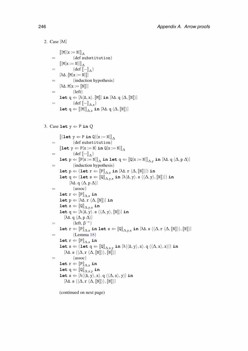
246 Appendix A. Arrow proofs
2. Case [M]
J[M][x := N]K∆= (def substitution)
J[M[x := N]]K∆= (def J−K∆)
[λ∆. JM[x := N]K]= (induction hypothesis)
[λ∆. M[x := JNK]]= (left)
let q⇐ [λ〈∆, x〉. JMK] in [λ∆. q 〈∆, JNK〉]= (def J−K∆,x)
let q⇐ J[M]K∆,x in [λ∆. q 〈∆, JNK〉]
3. Case let y⇐ P in Q
J(let y⇐ P in Q)[x := N]K∆= (def substitution)
Jlet y⇐ P[x := N] in Q[x := N]K∆= (def J−K∆)
let p⇐ JP[x := N]K∆ in let q⇐ JQ[x := N]K∆,y in [λ∆. q 〈∆, p ∆〉]= (induction hypothesis)
let p⇐ (let r⇐ JPK∆,x in [λ∆. r 〈∆, JNK〉]) inlet q⇐ (let s⇐ JQK∆,y,x in [λ〈∆, y〉. s 〈〈∆, y〉, JNK〉]) in
[λ∆. q 〈∆, p ∆〉]= (assoc)
let r⇐ JPK∆,x inlet p⇐ [λ∆. r 〈∆, JNK〉] inlet s⇐ JQK∆,y,x inlet q⇐ [λ〈∆, y〉. s 〈〈∆, y〉, JNK〉] in
[λ∆. q 〈∆, p ∆〉]= (left,β→)
let r⇐ JPK∆,x in let s⇐ JQK∆,y,x in [λ∆. s 〈〈∆, r 〈∆, JNK〉〉, JNK〉]= (Lemma 18)
let r⇐ JPK∆,x inlet s⇐ (let q⇐ JQK∆,x,y in [λ〈〈∆, y〉, x〉. q 〈〈∆, x〉, x〉]) in[λ∆. s 〈〈∆, r 〈∆, JNK〉〉, JNK〉]
= (assoc)let r⇐ JPK∆,x inlet q⇐ JQK∆,x,y inlet s⇐ [λ〈〈∆, y〉, x〉. q 〈〈∆, x〉, y〉] in[λ∆. s 〈〈∆, r 〈∆, JNK〉〉, JNK〉]
(continued on next page)
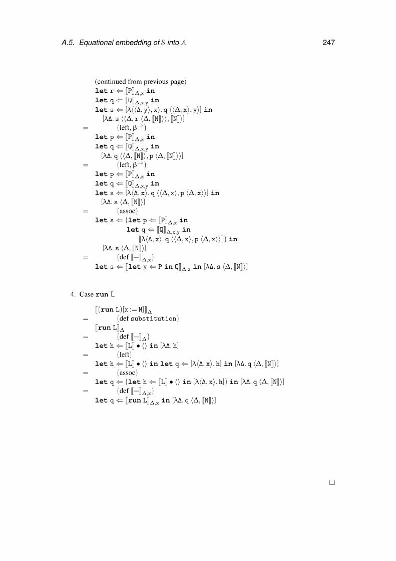
A.5. Equational embedding of S into A 247
(continued from previous page)let r⇐ JPK∆,x inlet q⇐ JQK∆,x,y inlet s⇐ [λ〈〈∆, y〉, x〉. q 〈〈∆, x〉, y〉] in[λ∆. s 〈〈∆, r 〈∆, JNK〉〉, JNK〉]
= (left,β→)let p⇐ JPK∆,x inlet q⇐ JQK∆,x,y in[λ∆. q 〈〈∆, JNK〉, p 〈∆, JNK〉〉]
= (left,β→)let p⇐ JPK∆,x inlet q⇐ JQK∆,x,y inlet s⇐ [λ〈∆, x〉. q 〈〈∆, x〉, p 〈∆, x〉〉] in[λ∆. s 〈∆, JNK〉]
= (assoc)let s⇐ (let p⇐ JPK∆,x in
let q⇐ JQK∆,x,y inJλ〈∆, x〉. q 〈〈∆, x〉, p 〈∆, x〉〉K) in
[λ∆. s 〈∆, JNK〉]= (def J−K∆,x)
let s⇐ Jlet y⇐ P in QK∆,x in [λ∆. s 〈∆, JNK〉]
4. Case run L
J(run L)[x := N]K∆= (def substitution)
Jrun LK∆= (def J−K∆)
let h⇐ JLK • 〈〉 in [λ∆. h]= (left)
let h⇐ JLK • 〈〉 in let q⇐ [λ〈∆, x〉. h] in [λ∆. q 〈∆, JNK〉]= (assoc)
let q⇐ (let h⇐ JLK • 〈〉 in [λ〈∆, x〉. h]) in [λ∆. q 〈∆, JNK〉]= (def J−K∆,x)
let q⇐ Jrun LK∆,x in [λ∆. q 〈∆, JNK〉]
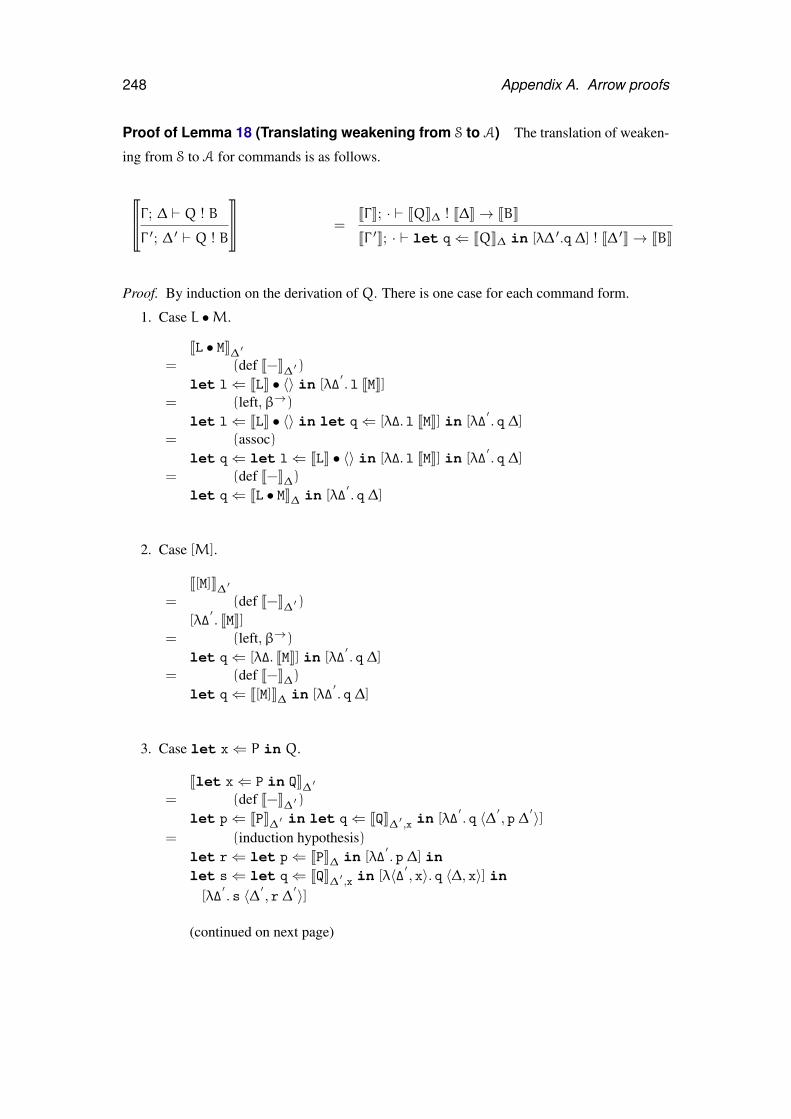
248 Appendix A. Arrow proofs
Proof of Lemma 18 (Translating weakening from S to A) The translation of weaken-
ing from S to A for commands is as follows.
u
vΓ ; ∆ ` Q ! B
Γ ′; ∆ ′ ` Q ! B
}
~ =JΓK; · ` JQK∆ ! J∆K→ JBK
JΓ ′K; · ` let q⇐ JQK∆ in [λ∆ ′.q ∆] ! J∆ ′K→ JBK
Proof. By induction on the derivation of Q. There is one case for each command form.
1. Case L •M.
JL • MK∆ ′= (def J−K∆ ′ )
let l⇐ JLK • 〈〉 in [λ∆′. l JMK]
= (left,β→)
let l⇐ JLK • 〈〉 in let q⇐ [λ∆. l JMK] in [λ∆′. q ∆]
= (assoc)let q⇐ let l⇐ JLK • 〈〉 in [λ∆. l JMK] in [λ∆
′. q ∆]
= (def J−K∆)let q⇐ JL • MK∆ in [λ∆
′. q ∆]
2. Case [M].
J[M]K∆ ′= (def J−K∆ ′ )
[λ∆′. JMK]
= (left,β→)
let q⇐ [λ∆. JMK] in [λ∆′. q ∆]
= (def J−K∆)let q⇐ J[M]K∆ in [λ∆
′. q ∆]
3. Case let x⇐ P in Q.
Jlet x⇐ P in QK∆ ′= (def J−K∆ ′ )
let p⇐ JPK∆ ′ in let q⇐ JQK∆ ′ ,x in [λ∆′. q 〈∆ ′ , p ∆ ′〉]
= (induction hypothesis)let r⇐ let p⇐ JPK∆ in [λ∆
′. p ∆] in
let s⇐ let q⇐ JQK∆ ′ ,x in [λ〈∆ ′ , x〉. q 〈∆, x〉] in[λ∆
′. s 〈∆ ′ , r ∆ ′〉]
(continued on next page)
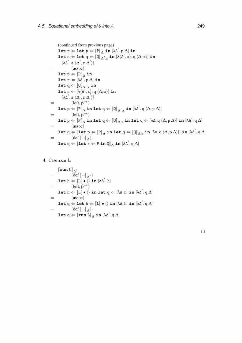
A.5. Equational embedding of S into A 249
(continued from previous page)let r⇐ let p⇐ JPK∆ in [λ∆
′. p ∆] in
let s⇐ let q⇐ JQK∆ ′ ,x in [λ〈∆ ′ , x〉. q 〈∆, x〉] in[λ∆
′. s 〈∆ ′ , r ∆ ′〉]
= (assoc)let p⇐ JPK∆ inlet r⇐ [λ∆
′. p ∆] in
let q⇐ JQK∆ ′ ,x inlet s⇐ [λ〈∆ ′ , x〉. q 〈∆, x〉] in[λ∆
′. s 〈∆ ′ , r ∆ ′〉]
= (left,β→)
let p⇐ JPK∆ in let q⇐ JQK∆ ′ ,x in [λ∆′. q 〈∆, p ∆〉]
= (left,β→)
let p⇐ JPK∆ in let q⇐ JQK∆,x in let q⇐ [λ∆. q 〈∆, p ∆〉] in [λ∆′. q ∆]
= (assoc)let q⇐ (let p⇐ JPK∆ in let q⇐ JQK∆,x in [λ∆. q 〈∆, p ∆〉]) in [λ∆
′. q ∆]
= (def J−K∆)let q⇐ Jlet x⇐ P in QK∆ in [λ∆
′. q ∆]
4. Case run L.
Jrun LK∆ ′= (def J−K∆ ′ )
let h⇐ JLK • 〈〉 in [λ∆′. h]
= (left,β→)
let h⇐ JLK • 〈〉 in let q⇐ [λ∆. h] in [λ∆′. q ∆]
= (assoc)let q⇐ let h⇐ JLK • 〈〉 in [λ∆. h] in [λ∆
′. q ∆]
= (def J−K∆)let q⇐ Jrun LK∆ in [λ∆
′. q ∆]
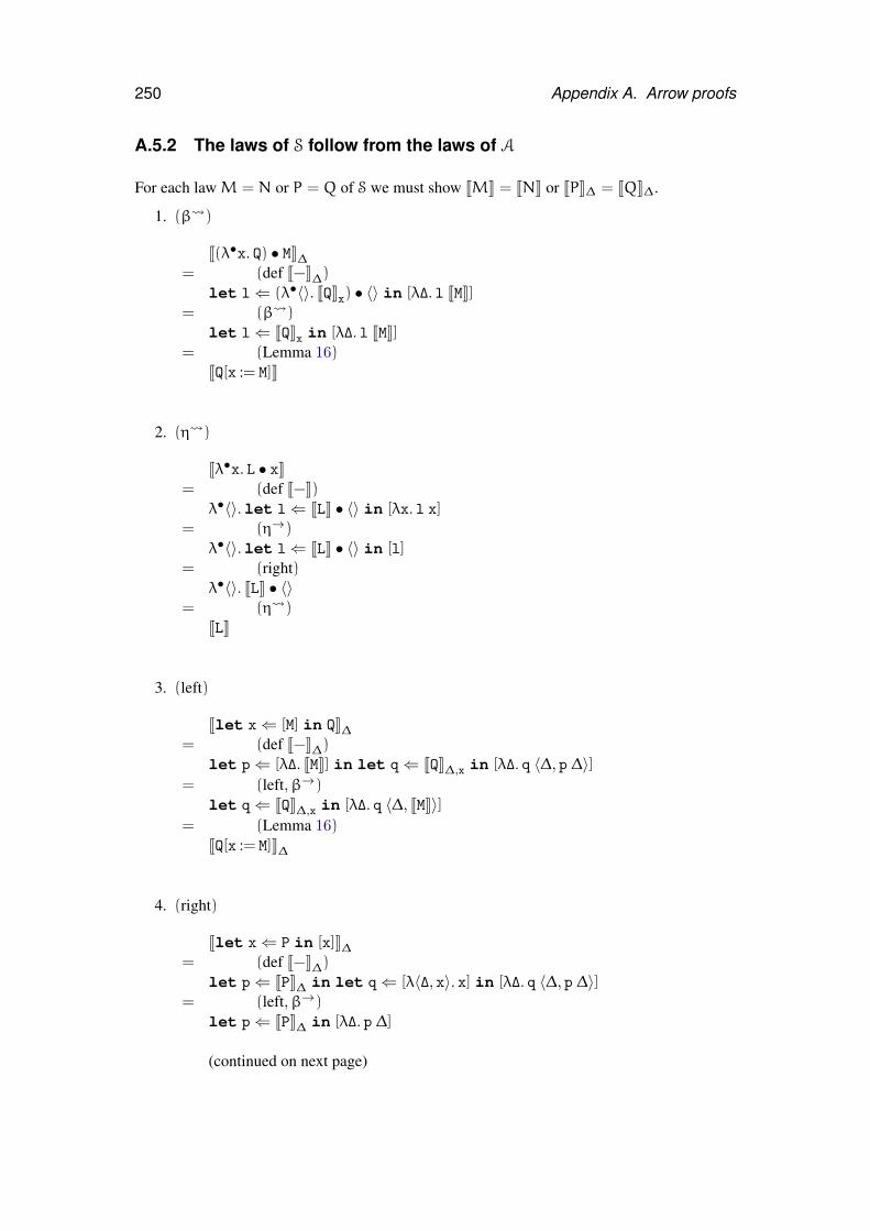
250 Appendix A. Arrow proofs
A.5.2 The laws of S follow from the laws of A
For each lawM = N or P = Q of S we must show JMK = JNK or JPK∆ = JQK∆.
1. (β )
J(λ•x. Q) • MK∆= (def J−K∆)
let l⇐ (λ•〈〉. JQKx) • 〈〉 in [λ∆. l JMK]= (β )
let l⇐ JQKx in [λ∆. l JMK]= (Lemma 16)
JQ[x := M]K
2. (η )
Jλ•x. L • xK= (def J−K)
λ•〈〉.let l⇐ JLK • 〈〉 in [λx. l x]= (η→)
λ•〈〉.let l⇐ JLK • 〈〉 in [l]= (right)
λ•〈〉. JLK • 〈〉= (η )
JLK
3. (left)
Jlet x⇐ [M] in QK∆= (def J−K∆)
let p⇐ [λ∆. JMK] in let q⇐ JQK∆,x in [λ∆. q 〈∆, p ∆〉]= (left,β→)
let q⇐ JQK∆,x in [λ∆. q 〈∆, JMK〉]= (Lemma 16)
JQ[x := M]K∆
4. (right)
Jlet x⇐ P in [x]K∆= (def J−K∆)
let p⇐ JPK∆ in let q⇐ [λ〈∆, x〉. x] in [λ∆. q 〈∆, p ∆〉]= (left,β→)
let p⇐ JPK∆ in [λ∆. p ∆]
(continued on next page)
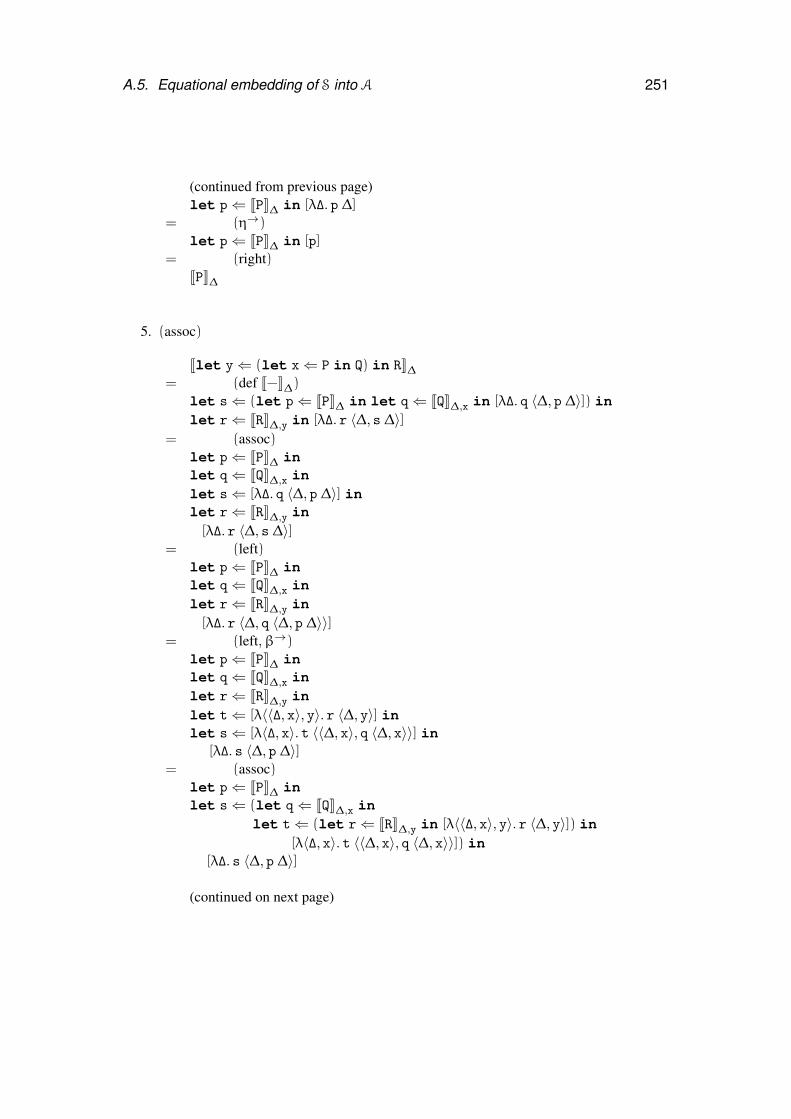
A.5. Equational embedding of S into A 251
(continued from previous page)let p⇐ JPK∆ in [λ∆. p ∆]
= (η→)let p⇐ JPK∆ in [p]
= (right)JPK∆
5. (assoc)
Jlet y⇐ (let x⇐ P in Q) in RK∆= (def J−K∆)
let s⇐ (let p⇐ JPK∆ in let q⇐ JQK∆,x in [λ∆. q 〈∆, p ∆〉]) inlet r⇐ JRK∆,y in [λ∆. r 〈∆, s ∆〉]
= (assoc)let p⇐ JPK∆ inlet q⇐ JQK∆,x inlet s⇐ [λ∆. q 〈∆, p ∆〉] inlet r⇐ JRK∆,y in[λ∆. r 〈∆, s ∆〉]
= (left)let p⇐ JPK∆ inlet q⇐ JQK∆,x inlet r⇐ JRK∆,y in[λ∆. r 〈∆, q 〈∆, p ∆〉〉]
= (left,β→)let p⇐ JPK∆ inlet q⇐ JQK∆,x inlet r⇐ JRK∆,y inlet t⇐ [λ〈〈∆, x〉, y〉. r 〈∆, y〉] inlet s⇐ [λ〈∆, x〉. t 〈〈∆, x〉, q 〈∆, x〉〉] in
[λ∆. s 〈∆, p ∆〉]= (assoc)
let p⇐ JPK∆ inlet s⇐ (let q⇐ JQK∆,x in
let t⇐ (let r⇐ JRK∆,y in [λ〈〈∆, x〉, y〉. r 〈∆, y〉]) in[λ〈∆, x〉. t 〈〈∆, x〉, q 〈∆, x〉〉]) in
[λ∆. s 〈∆, p ∆〉]
(continued on next page)
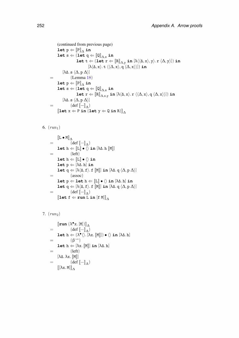
252 Appendix A. Arrow proofs
(continued from previous page)let p⇐ JPK∆ inlet s⇐ (let q⇐ JQK∆,x in
let t⇐ (let r⇐ JRK∆,y in [λ〈〈∆, x〉, y〉. r 〈∆, y〉]) in[λ〈∆, x〉. t 〈〈∆, x〉, q 〈∆, x〉〉]) in
[λ∆. s 〈∆, p ∆〉]= (Lemma 18)
let p⇐ JPK∆ inlet s⇐ (let q⇐ JQK∆,x in
let r⇐ JRK∆,x,y in [λ〈∆, x〉. r 〈〈∆, x〉, q 〈∆, x〉〉]) in[λ∆. s 〈∆, p ∆〉]
= (def J−K∆)Jlet x⇐ P in (let y⇐ Q in R)K∆
6. (run1)
JL • MK∆= (def J−K∆)
let h⇐ JLK • 〈〉 in [λ∆. h JMK]= (left)
let h⇐ JLK • 〈〉 inlet p⇐ [λ∆. h] inlet q⇐ [λ〈∆, f〉. f JMK] in [λ∆. q 〈∆, p ∆〉]
= (assoc)let p⇐ let h⇐ JLK • 〈〉 in [λ∆. h] inlet q⇐ [λ〈∆, f〉. f JMK] in [λ∆. q 〈∆, p ∆〉]
= (def J−K∆)Jlet f⇐ run L in [f M]K∆
7. (run2)
Jrun (λ•x. [M])K∆= (def J−K∆)
let h⇐ (λ•〈〉. [λx. JMK]) • 〈〉 in [λ∆. h]= (β )
let h⇐ [λx. JMK] in [λ∆. h]= (left)
[λ∆. λx. JMK]= (def J−K∆)
J[λx. M]K∆
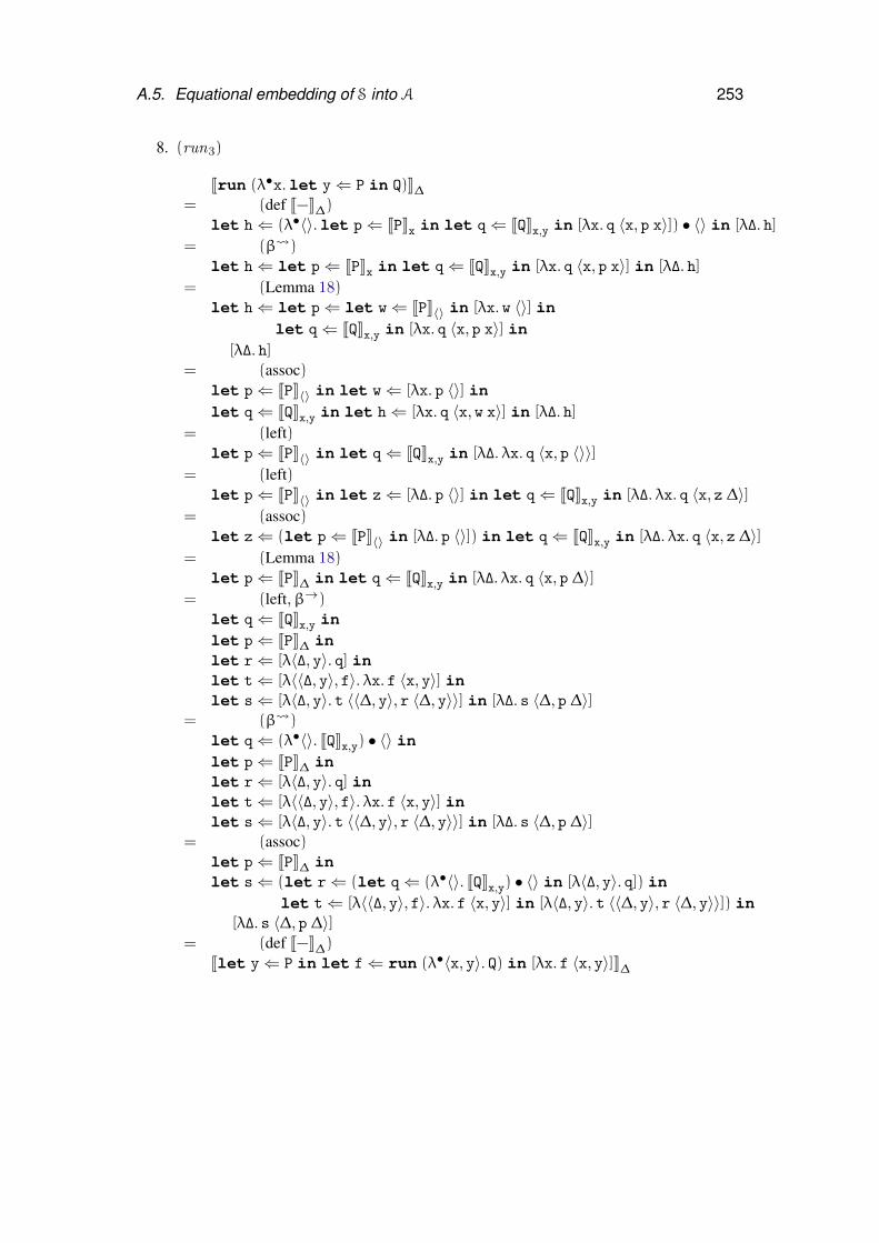
A.5. Equational embedding of S into A 253
8. (run3)
Jrun (λ•x.let y⇐ P in Q)K∆= (def J−K∆)
let h⇐ (λ•〈〉.let p⇐ JPKx in let q⇐ JQKx,y in [λx. q 〈x, p x〉]) • 〈〉 in [λ∆. h]
= (β )let h⇐ let p⇐ JPKx in let q⇐ JQKx,y in [λx. q 〈x, p x〉] in [λ∆. h]
= (Lemma 18)let h⇐ let p⇐ let w⇐ JPK〈〉 in [λx. w 〈〉] in
let q⇐ JQKx,y in [λx. q 〈x, p x〉] in[λ∆. h]
= (assoc)let p⇐ JPK〈〉 in let w⇐ [λx. p 〈〉] inlet q⇐ JQKx,y in let h⇐ [λx. q 〈x, w x〉] in [λ∆. h]
= (left)let p⇐ JPK〈〉 in let q⇐ JQKx,y in [λ∆. λx. q 〈x, p 〈〉〉]
= (left)let p⇐ JPK〈〉 in let z⇐ [λ∆. p 〈〉] in let q⇐ JQKx,y in [λ∆. λx. q 〈x, z ∆〉]
= (assoc)let z⇐ (let p⇐ JPK〈〉 in [λ∆. p 〈〉]) in let q⇐ JQKx,y in [λ∆. λx. q 〈x, z ∆〉]
= (Lemma 18)let p⇐ JPK∆ in let q⇐ JQKx,y in [λ∆. λx. q 〈x, p ∆〉]
= (left,β→)let q⇐ JQKx,y inlet p⇐ JPK∆ inlet r⇐ [λ〈∆, y〉. q] inlet t⇐ [λ〈〈∆, y〉, f〉. λx. f 〈x, y〉] inlet s⇐ [λ〈∆, y〉. t 〈〈∆, y〉, r 〈∆, y〉〉] in [λ∆. s 〈∆, p ∆〉]
= (β )let q⇐ (λ•〈〉. JQKx,y) • 〈〉 inlet p⇐ JPK∆ inlet r⇐ [λ〈∆, y〉. q] inlet t⇐ [λ〈〈∆, y〉, f〉. λx. f 〈x, y〉] inlet s⇐ [λ〈∆, y〉. t 〈〈∆, y〉, r 〈∆, y〉〉] in [λ∆. s 〈∆, p ∆〉]
= (assoc)let p⇐ JPK∆ inlet s⇐ (let r⇐ (let q⇐ (λ•〈〉. JQKx,y) • 〈〉 in [λ〈∆, y〉. q]) in
let t⇐ [λ〈〈∆, y〉, f〉. λx. f 〈x, y〉] in [λ〈∆, y〉. t 〈〈∆, y〉, r 〈∆, y〉〉]) in[λ∆. s 〈∆, p ∆〉]
= (def J−K∆)Jlet y⇐ P in let f⇐ run (λ•〈x, y〉. Q) in [λx. f 〈x, y〉]K∆
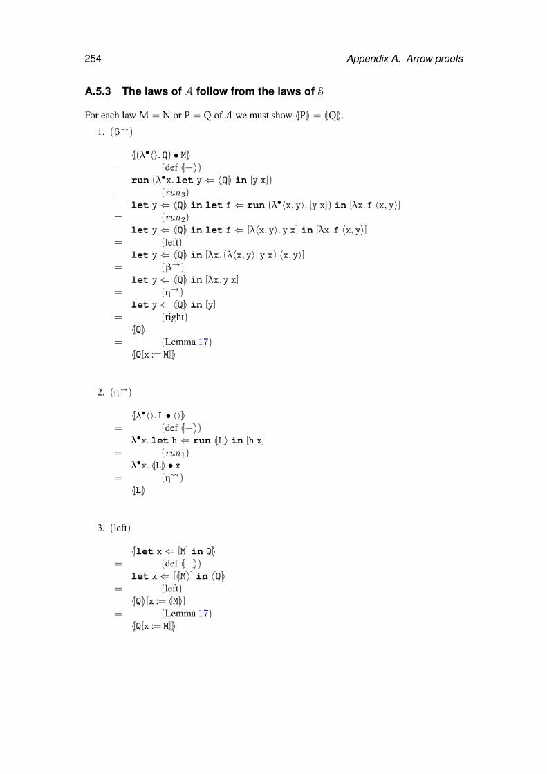
254 Appendix A. Arrow proofs
A.5.3 The laws of A follow from the laws of S
For each lawM = N or P = Q of A we must show 〈[P]〉 = 〈[Q]〉.1. (β )
〈[(λ•〈〉. Q) • M]〉= (def 〈[−]〉)
run (λ•x.let y⇐ 〈[Q]〉 in [y x])= (run3)
let y⇐ 〈[Q]〉 in let f⇐ run (λ•〈x, y〉. [y x]) in [λx. f 〈x, y〉]= (run2)
let y⇐ 〈[Q]〉 in let f⇐ [λ〈x, y〉. y x] in [λx. f 〈x, y〉]= (left)
let y⇐ 〈[Q]〉 in [λx. (λ〈x, y〉. y x) 〈x, y〉]= (β→)
let y⇐ 〈[Q]〉 in [λx. y x]= (η→)
let y⇐ 〈[Q]〉 in [y]= (right)〈[Q]〉
= (Lemma 17)〈[Q[x := M]]〉
2. (η )
〈[λ•〈〉. L • 〈〉]〉= (def 〈[−]〉)
λ•x.let h⇐ run 〈[L]〉 in [h x]= (run1)
λ•x. 〈[L]〉 • x= (η )〈[L]〉
3. (left)
〈[let x⇐ [M] in Q]〉= (def 〈[−]〉)
let x⇐ [〈[M]〉] in 〈[Q]〉= (left)〈[Q]〉[x := 〈[M]〉]
= (Lemma 17)〈[Q[x := M]]〉
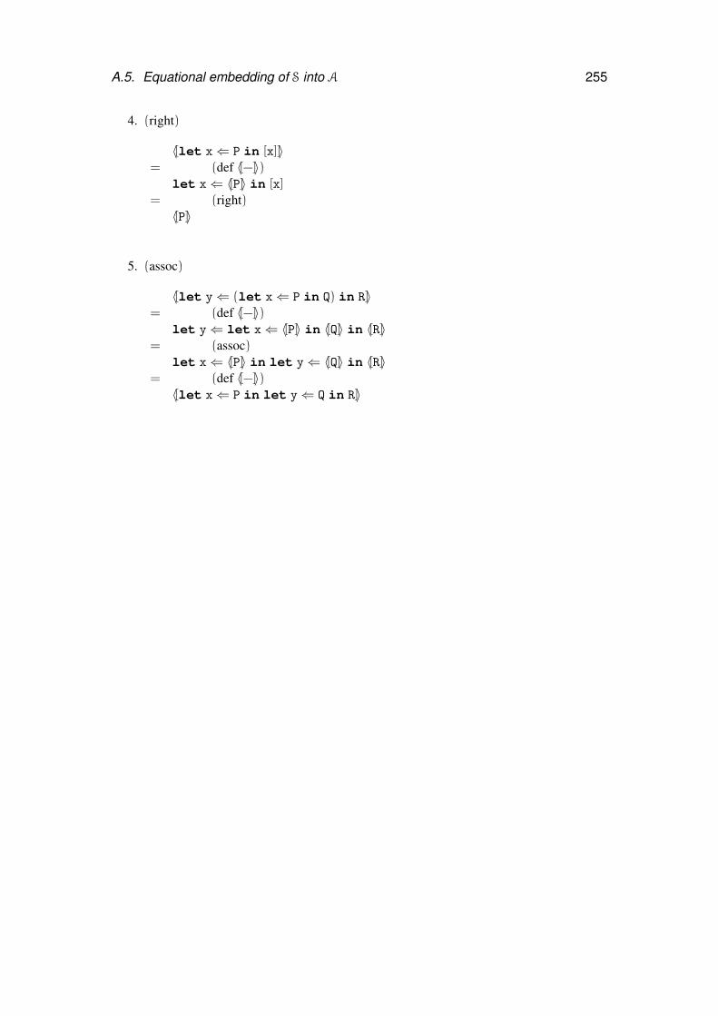
A.5. Equational embedding of S into A 255
4. (right)
〈[let x⇐ P in [x]]〉= (def 〈[−]〉)
let x⇐ 〈[P]〉 in [x]= (right)〈[P]〉
5. (assoc)
〈[let y⇐ (let x⇐ P in Q) in R]〉= (def 〈[−]〉)
let y⇐ let x⇐ 〈[P]〉 in 〈[Q]〉 in 〈[R]〉= (assoc)
let x⇐ 〈[P]〉 in let y⇐ 〈[Q]〉 in 〈[R]〉= (def 〈[−]〉)〈[let x⇐ P in let y⇐ Q in R]〉
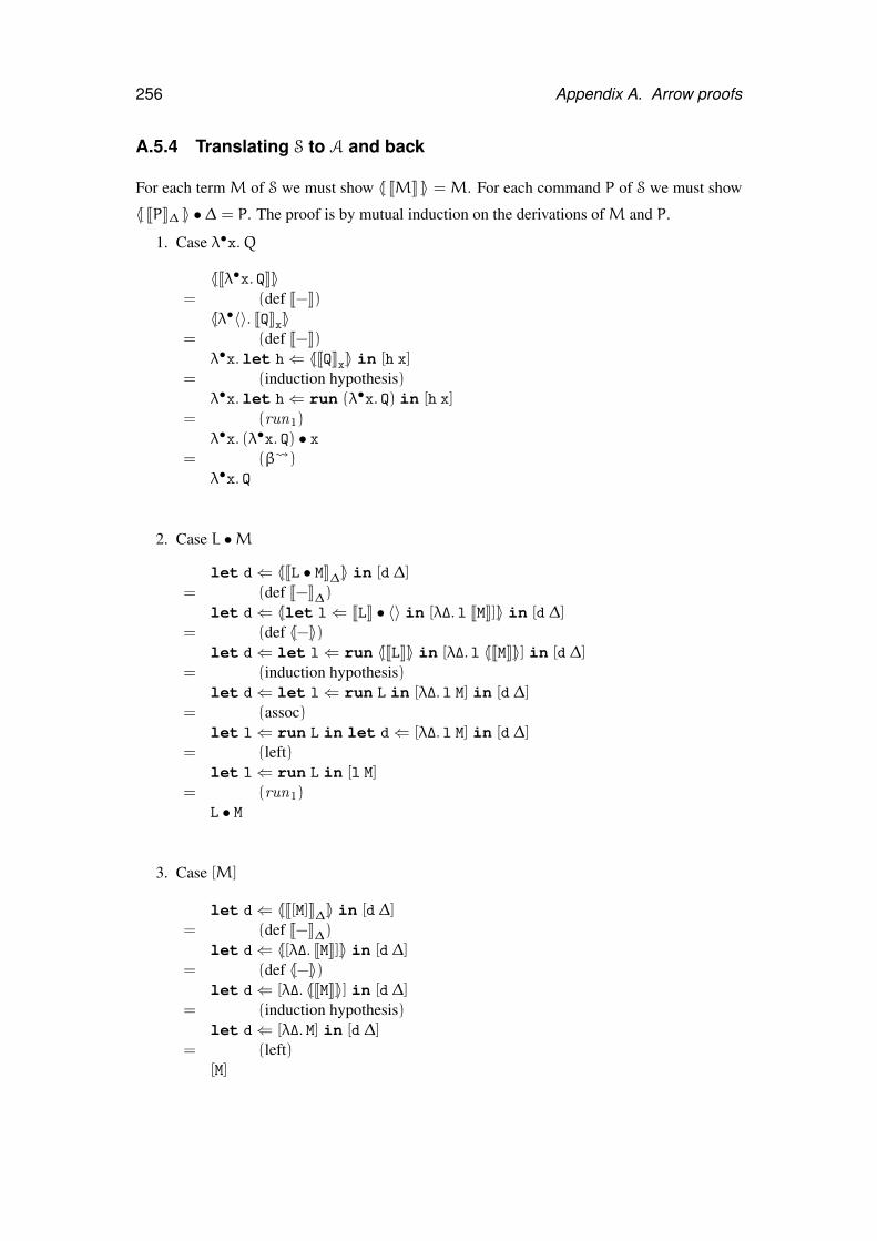
256 Appendix A. Arrow proofs
A.5.4 Translating S to A and back
For each term M of S we must show 〈[ JMK ]〉 =M. For each command P of S we must show
〈[ JPK∆ ]〉 • ∆ = P. The proof is by mutual induction on the derivations ofM and P.
1. Case λ•x.Q
〈[Jλ•x. QK]〉= (def J−K)〈[λ•〈〉. JQKx]〉
= (def J−K)λ•x.let h⇐ 〈[JQKx]〉 in [h x]
= (induction hypothesis)λ•x.let h⇐ run (λ•x. Q) in [h x]
= (run1)λ•x. (λ•x. Q) • x
= (β )λ•x. Q
2. Case L •M
let d⇐ 〈[JL • MK∆]〉 in [d ∆]= (def J−K∆)
let d⇐ 〈[let l⇐ JLK • 〈〉 in [λ∆. l JMK]]〉 in [d ∆]= (def 〈[−]〉)
let d⇐ let l⇐ run 〈[JLK]〉 in [λ∆. l 〈[JMK]〉] in [d ∆]= (induction hypothesis)
let d⇐ let l⇐ run L in [λ∆. l M] in [d ∆]= (assoc)
let l⇐ run L in let d⇐ [λ∆. l M] in [d ∆]= (left)
let l⇐ run L in [l M]= (run1)
L • M
3. Case [M]
let d⇐ 〈[J[M]K∆]〉 in [d ∆]= (def J−K∆)
let d⇐ 〈[[λ∆. JMK]]〉 in [d ∆]= (def 〈[−]〉)
let d⇐ [λ∆. 〈[JMK]〉] in [d ∆]= (induction hypothesis)
let d⇐ [λ∆. M] in [d ∆]= (left)
[M]
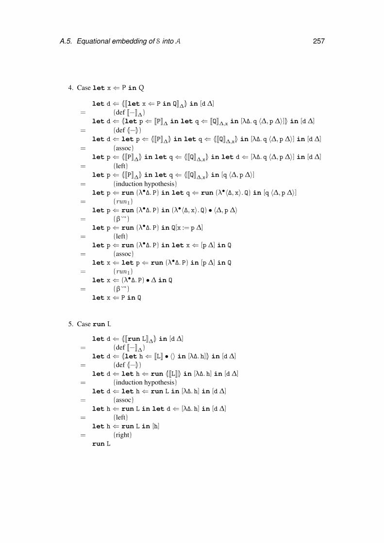
A.5. Equational embedding of S into A 257
4. Case let x⇐ P in Q
let d⇐ 〈[Jlet x⇐ P in QK∆]〉 in [d ∆]= (def J−K∆)
let d⇐ 〈[let p⇐ JPK∆ in let q⇐ JQK∆,x in [λ∆. q 〈∆, p ∆〉]]〉 in [d ∆]
= (def 〈[−]〉)let d⇐ let p⇐ 〈[JPK∆]〉 in let q⇐ 〈[JQK∆,x]〉 in [λ∆. q 〈∆, p ∆〉] in [d ∆]
= (assoc)let p⇐ 〈[JPK∆]〉 in let q⇐ 〈[JQK∆,x]〉 in let d⇐ [λ∆. q 〈∆, p ∆〉] in [d ∆]
= (left)let p⇐ 〈[JPK∆]〉 in let q⇐ 〈[JQK∆,x]〉 in [q 〈∆, p ∆〉]
= (induction hypothesis)let p⇐ run (λ•∆. P) in let q⇐ run (λ•〈∆, x〉. Q) in [q 〈∆, p ∆〉]
= (run1)let p⇐ run (λ•∆. P) in (λ•〈∆, x〉. Q) • 〈∆, p ∆〉
= (β )let p⇐ run (λ•∆. P) in Q[x := p ∆]
= (left)let p⇐ run (λ•∆. P) in let x⇐ [p ∆] in Q
= (assoc)let x⇐ let p⇐ run (λ•∆. P) in [p ∆] in Q
= (run1)let x⇐ (λ•∆. P) • ∆ in Q
= (β )let x⇐ P in Q
5. Case run L
let d⇐ 〈[Jrun LK∆]〉 in [d ∆]= (def J−K∆)
let d⇐ 〈[let h⇐ JLK • 〈〉 in [λ∆. h]]〉 in [d ∆]= (def 〈[−]〉)
let d⇐ let h⇐ run 〈[JLK]〉 in [λ∆. h] in [d ∆]= (induction hypothesis)
let d⇐ let h⇐ run L in [λ∆. h] in [d ∆]= (assoc)
let h⇐ run L in let d⇐ [λ∆. h] in [d ∆]= (left)
let h⇐ run L in [h]= (right)
run L
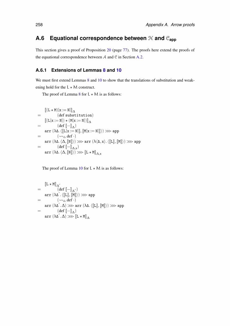
258 Appendix A. Arrow proofs
A.6 Equational correspondence between H and Capp
This section gives a proof of Proposition 20 (page 77). The proofs here extend the proofs of
the equational correspondence between A and C in Section A.2.
A.6.1 Extensions of Lemmas 8 and 10
We must first extend Lemmas 8 and 10 to show that the translations of substitution and weak-
ening hold for the L ?M construct.
The proof of Lemma 8 for L ?M is as follows:
J(L ? M)[x := N]K∆= (def substitution)
J(L[x := N]) ? (M[x := N])K∆= (def J−K∆)
arr (λ∆. 〈JL[x := N]K, JM[x := N]K〉)>>> app
= ( 4, def ·)arr (λ∆. 〈∆, JNK〉)>>> arr (λ〈∆, x〉. 〈JLK, JMK〉)>>> app
= (def J−K∆,x)
arr (λ∆. 〈∆, JNK〉)>>> JL ? MK∆,x
The proof of Lemma 10 for L ?M is as follows:
JL ? MK∆ ′= (def J−K∆ ′ )
arr (λ∆′. 〈JLK, JMK〉)>>> app
= ( 4, def ·)arr (λ∆
′.∆)>>> arr (λ∆. 〈JLK, JMK〉)>>> app
= (def J−K∆)arr (λ∆
′.∆)>>> JL ? MK∆
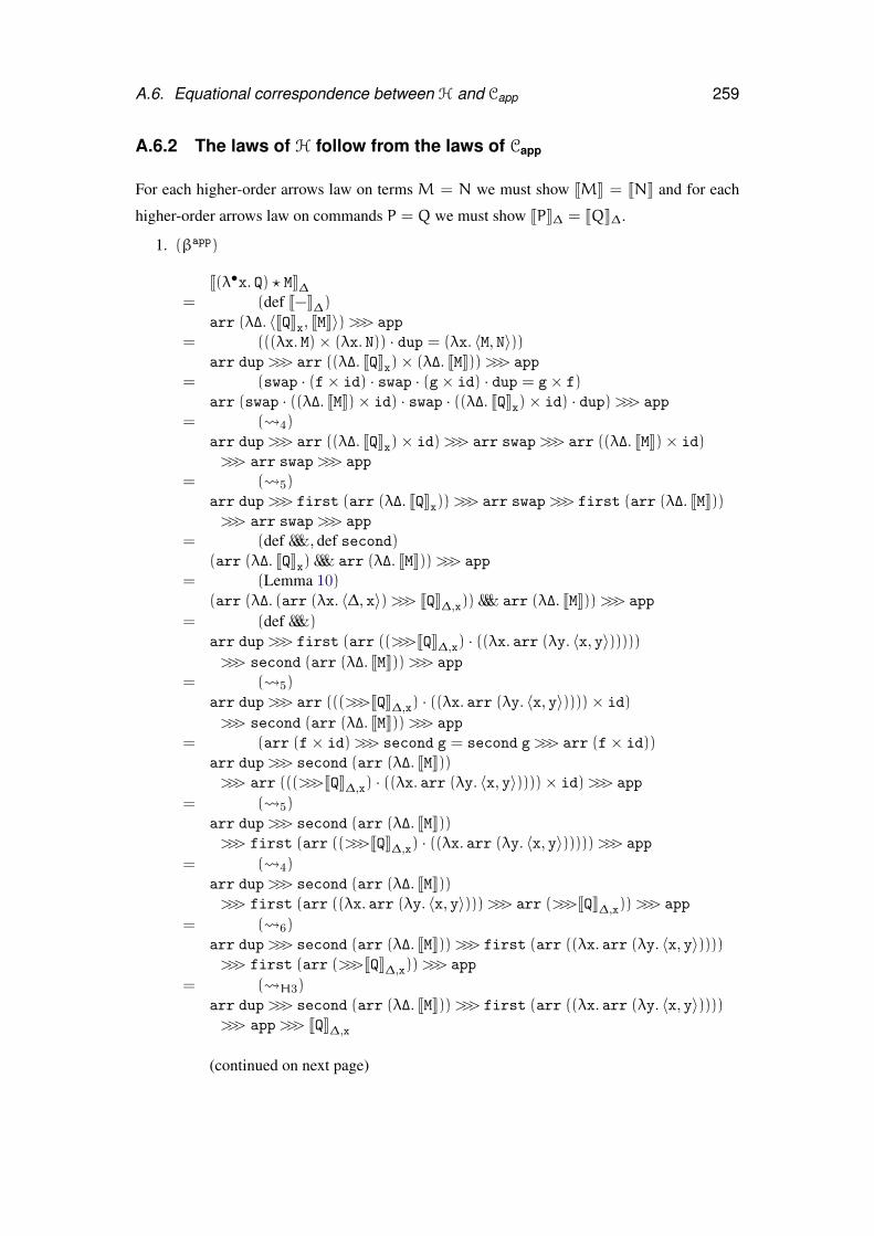
A.6. Equational correspondence between H and Capp 259
A.6.2 The laws of H follow from the laws of Capp
For each higher-order arrows law on terms M = N we must show JMK = JNK and for each
higher-order arrows law on commands P = Q we must show JPK∆ = JQK∆.
1. (βapp)
J(λ•x. Q) ? MK∆= (def J−K∆)
arr (λ∆. 〈JQKx, JMK〉)>>> app
= (((λx. M)× (λx. N)) · dup = (λx. 〈M, N〉))arr dup>>> arr ((λ∆. JQKx)× (λ∆. JMK))>>> app
= (swap · (f× id) · swap · (g× id) · dup = g× f)arr (swap · ((λ∆. JMK)× id) · swap · ((λ∆. JQKx)× id) · dup)>>> app
= ( 4)arr dup>>> arr ((λ∆. JQKx)× id)>>> arr swap>>> arr ((λ∆. JMK)× id)>>> arr swap>>> app
= ( 5)arr dup>>> first (arr (λ∆. JQKx))>>> arr swap>>> first (arr (λ∆. JMK))>>> arr swap>>> app
= (def &&&, def second)(arr (λ∆. JQKx) &&& arr (λ∆. JMK))>>> app
= (Lemma 10)(arr (λ∆. (arr (λx. 〈∆, x〉)>>> JQK∆,x)) &&& arr (λ∆. JMK))>>> app
= (def &&&)arr dup>>> first (arr ((>>>JQK∆,x) · ((λx. arr (λy. 〈x, y〉)))))>>> second (arr (λ∆. JMK))>>> app
= ( 5)arr dup>>> arr (((>>>JQK∆,x) · ((λx. arr (λy. 〈x, y〉))))× id)
>>> second (arr (λ∆. JMK))>>> app
= (arr (f× id)>>> second g = second g>>> arr (f× id))arr dup>>> second (arr (λ∆. JMK))>>> arr (((>>>JQK∆,x) · ((λx. arr (λy. 〈x, y〉))))× id)>>> app
= ( 5)arr dup>>> second (arr (λ∆. JMK))>>> first (arr ((>>>JQK∆,x) · ((λx. arr (λy. 〈x, y〉)))))>>> app
= ( 4)arr dup>>> second (arr (λ∆. JMK))>>> first (arr ((λx. arr (λy. 〈x, y〉)))>>> arr (>>>JQK∆,x))>>> app
= ( 6)arr dup>>> second (arr (λ∆. JMK))>>> first (arr ((λx. arr (λy. 〈x, y〉))))>>> first (arr (>>>JQK∆,x))>>> app
= ( H3)arr dup>>> second (arr (λ∆. JMK))>>> first (arr ((λx. arr (λy. 〈x, y〉))))>>> app>>> JQK∆,x
(continued on next page)
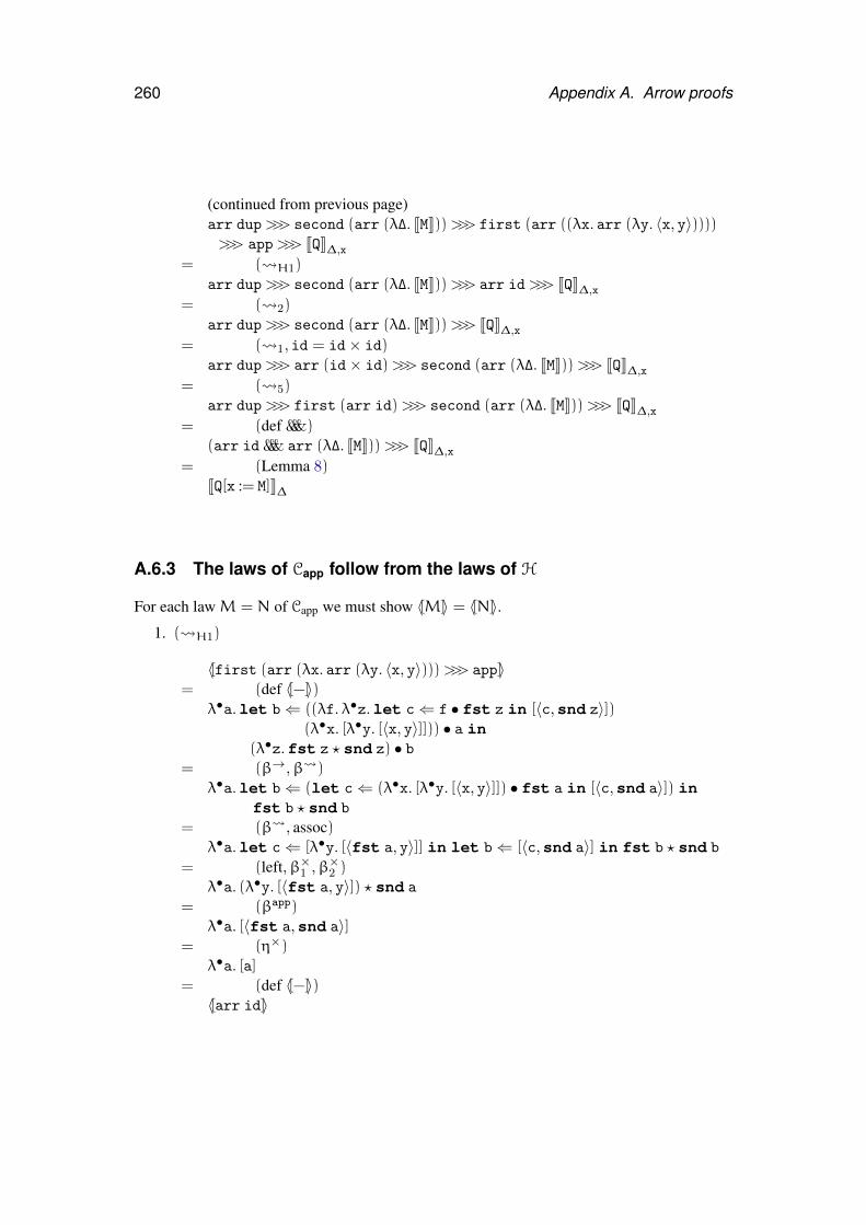
260 Appendix A. Arrow proofs
(continued from previous page)arr dup>>> second (arr (λ∆. JMK))>>> first (arr ((λx. arr (λy. 〈x, y〉))))>>> app>>> JQK∆,x
= ( H1)arr dup>>> second (arr (λ∆. JMK))>>> arr id>>> JQK∆,x
= ( 2)arr dup>>> second (arr (λ∆. JMK))>>> JQK∆,x
= ( 1, id = id× id)arr dup>>> arr (id× id)>>> second (arr (λ∆. JMK))>>> JQK∆,x
= ( 5)arr dup>>> first (arr id)>>> second (arr (λ∆. JMK))>>> JQK∆,x
= (def &&&)(arr id &&& arr (λ∆. JMK))>>> JQK∆,x
= (Lemma 8)JQ[x := M]K∆
A.6.3 The laws of Capp follow from the laws of H
For each lawM = N of Capp we must show 〈[M]〉 = 〈[N]〉.1. ( H1)
〈[first (arr (λx. arr (λy. 〈x, y〉)))>>> app]〉= (def 〈[−]〉)
λ•a.let b⇐ ((λf. λ•z.let c⇐ f • fst z in [〈c,snd z〉])(λ•x. [λ•y. [〈x, y〉]])) • a in
(λ•z.fst z ? snd z) • b= (β→,β )
λ•a.let b⇐ (let c⇐ (λ•x. [λ•y. [〈x, y〉]]) • fst a in [〈c,snd a〉]) infst b ? snd b
= (β , assoc)λ•a.let c⇐ [λ•y. [〈fst a, y〉]] in let b⇐ [〈c,snd a〉] in fst b ? snd b
= (left,β×1 ,β×2 )λ•a. (λ•y. [〈fst a, y〉]) ? snd a
= (βapp)λ•a. [〈fst a,snd a〉]
= (η×)λ•a. [a]
= (def 〈[−]〉)〈[arr id]〉
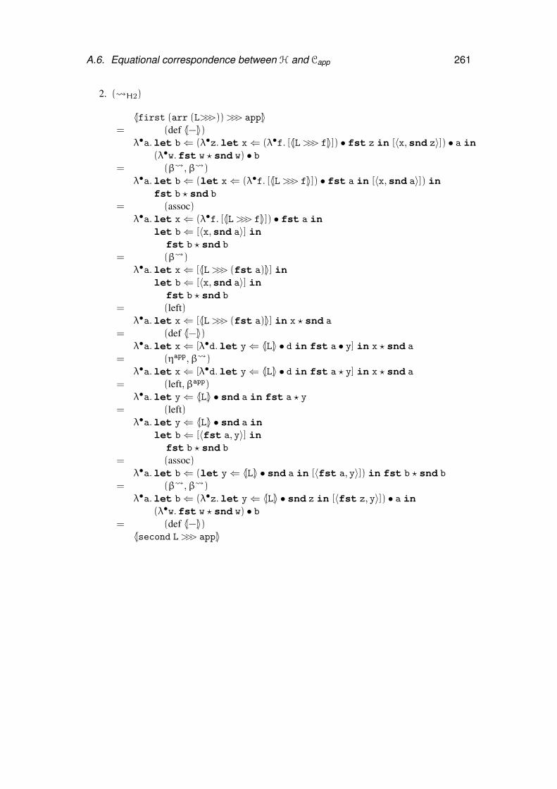
A.6. Equational correspondence between H and Capp 261
2. ( H2)
〈[first (arr (L>>>))>>> app]〉= (def 〈[−]〉)
λ•a.let b⇐ (λ•z.let x⇐ (λ•f. [〈[L>>> f]〉]) • fst z in [〈x,snd z〉]) • a in(λ•w.fst w ? snd w) • b
= (β ,β )λ•a.let b⇐ (let x⇐ (λ•f. [〈[L>>> f]〉]) • fst a in [〈x,snd a〉]) in
fst b ? snd b
= (assoc)λ•a.let x⇐ (λ•f. [〈[L>>> f]〉]) • fst a in
let b⇐ [〈x,snd a〉] infst b ? snd b
= (β )λ•a.let x⇐ [〈[L>>> (fst a)]〉] in
let b⇐ [〈x,snd a〉] infst b ? snd b
= (left)λ•a.let x⇐ [〈[L>>> (fst a)]〉] in x ? snd a
= (def 〈[−]〉)λ•a.let x⇐ [λ•d.let y⇐ 〈[L]〉 • d in fst a • y] in x ? snd a
= (ηapp,β )λ•a.let x⇐ [λ•d.let y⇐ 〈[L]〉 • d in fst a ? y] in x ? snd a
= (left,βapp)λ•a.let y⇐ 〈[L]〉 • snd a in fst a ? y
= (left)λ•a.let y⇐ 〈[L]〉 • snd a in
let b⇐ [〈fst a, y〉] infst b ? snd b
= (assoc)λ•a.let b⇐ (let y⇐ 〈[L]〉 • snd a in [〈fst a, y〉]) in fst b ? snd b
= (β ,β )λ•a.let b⇐ (λ•z.let y⇐ 〈[L]〉 • snd z in [〈fst z, y〉]) • a in
(λ•w.fst w ? snd w) • b= (def 〈[−]〉)〈[second L>>> app]〉
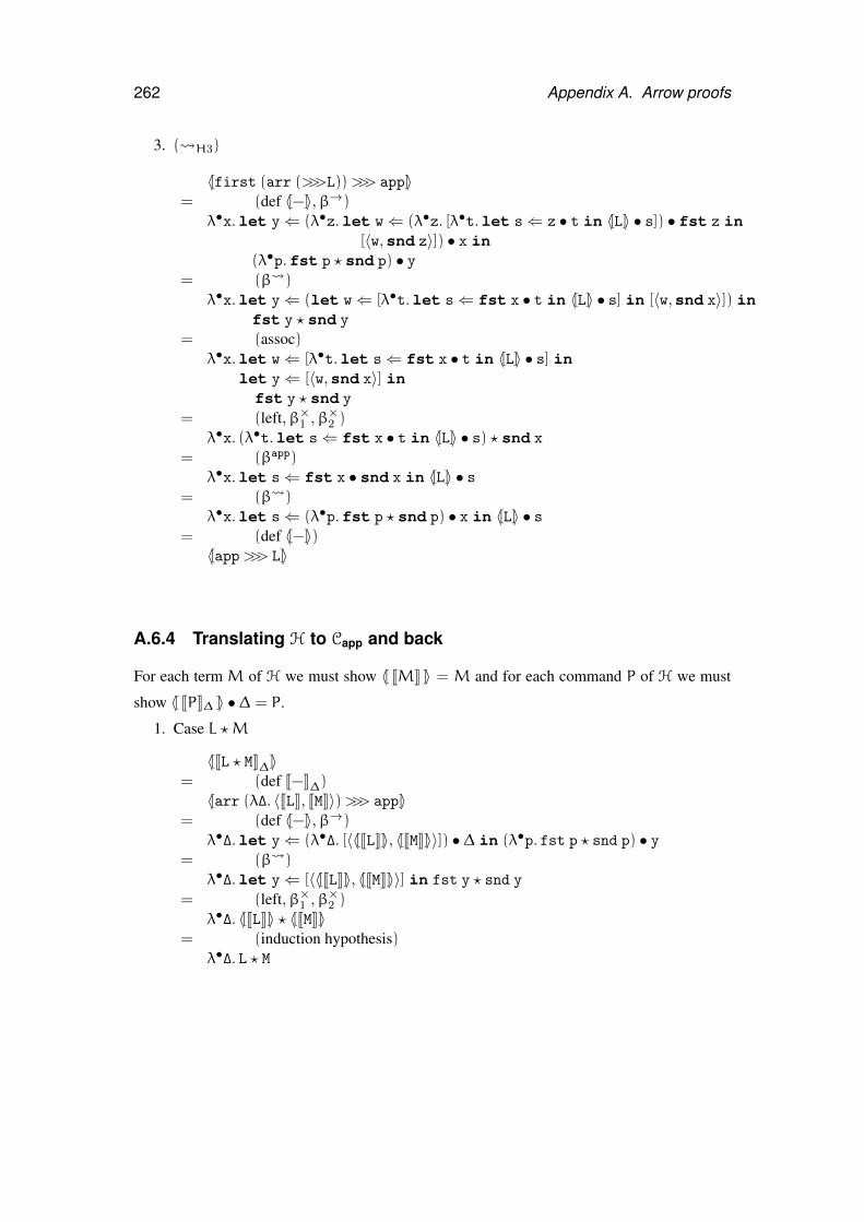
262 Appendix A. Arrow proofs
3. ( H3)
〈[first (arr (>>>L))>>> app]〉= (def 〈[−]〉,β→)
λ•x.let y⇐ (λ•z.let w⇐ (λ•z. [λ•t.let s⇐ z • t in 〈[L]〉 • s]) • fst z in[〈w,snd z〉]) • x in
(λ•p.fst p ? snd p) • y= (β )
λ•x.let y⇐ (let w⇐ [λ•t.let s⇐ fst x • t in 〈[L]〉 • s] in [〈w,snd x〉]) infst y ? snd y
= (assoc)λ•x.let w⇐ [λ•t.let s⇐ fst x • t in 〈[L]〉 • s] in
let y⇐ [〈w,snd x〉] infst y ? snd y
= (left,β×1 ,β×2 )λ•x. (λ•t.let s⇐ fst x • t in 〈[L]〉 • s) ? snd x
= (βapp)λ•x.let s⇐ fst x • snd x in 〈[L]〉 • s
= (β )λ•x.let s⇐ (λ•p.fst p ? snd p) • x in 〈[L]〉 • s
= (def 〈[−]〉)〈[app>>> L]〉
A.6.4 Translating H to Capp and back
For each term M of H we must show 〈[ JMK ]〉 = M and for each command P of H we must
show 〈[ JPK∆ ]〉 • ∆ = P.
1. Case L ?M
〈[JL ? MK∆]〉= (def J−K∆)〈[arr (λ∆. 〈JLK, JMK〉)>>> app]〉
= (def 〈[−]〉,β→)λ•∆.let y⇐ (λ•∆. [〈〈[JLK]〉, 〈[JMK]〉〉]) • ∆ in (λ•p. fst p ? snd p) • y
= (β )λ•∆.let y⇐ [〈〈[JLK]〉, 〈[JMK]〉〉] in fst y ? snd y
= (left,β×1 ,β×2 )λ•∆. 〈[JLK]〉 ? 〈[JMK]〉
= (induction hypothesis)λ•∆. L ? M
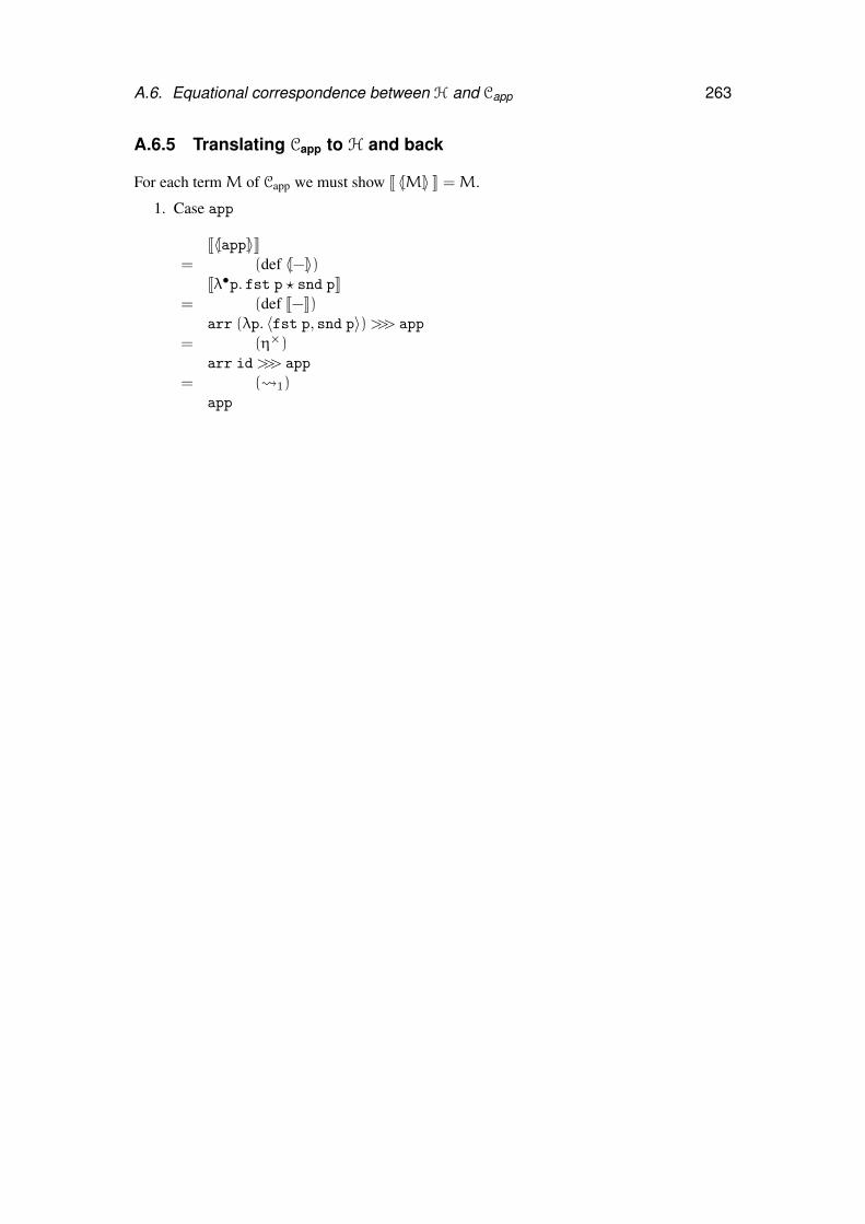
A.6. Equational correspondence between H and Capp 263
A.6.5 Translating Capp to H and back
For each termM of Capp we must show J 〈[M]〉 K =M.
1. Case app
J〈[app]〉K= (def 〈[−]〉)
Jλ•p. fst p ? snd pK= (def J−K)
arr (λp. 〈fst p, snd p〉)>>> app
= (η×)arr id>>> app
= ( 1)app
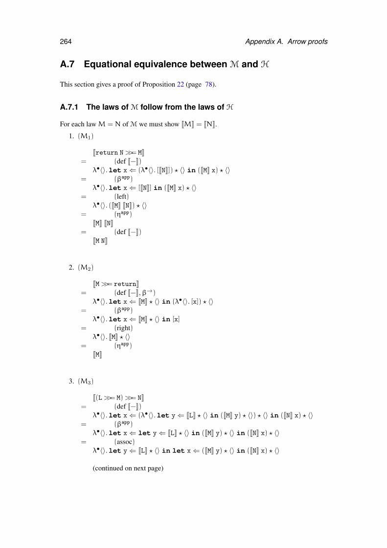
264 Appendix A. Arrow proofs
A.7 Equational equivalence between M and H
This section gives a proof of Proposition 22 (page 78).
A.7.1 The laws of M follow from the laws of H
For each lawM = N of M we must show JMK = JNK.
1. (M1)
Jreturn N>>= MK= (def J−K)
λ•〈〉.let x⇐ (λ•〈〉. [JNK]) ? 〈〉 in (JMK x) ? 〈〉= (βapp)
λ•〈〉.let x⇐ [JNK] in (JMK x) ? 〈〉= (left)
λ•〈〉. (JMK JNK) ? 〈〉= (ηapp)
JMK JNK= (def J−K)
JM NK
2. (M2)
JM>>= returnK= (def J−K,β→)
λ•〈〉.let x⇐ JMK ? 〈〉 in (λ•〈〉. [x]) ? 〈〉= (βapp)
λ•〈〉.let x⇐ JMK ? 〈〉 in [x]= (right)
λ•〈〉. JMK ? 〈〉= (ηapp)
JMK
3. (M3)
J(L>>= M)>>= NK= (def J−K)
λ•〈〉.let x⇐ (λ•〈〉.let y⇐ JLK ? 〈〉 in (JMK y) ? 〈〉) ? 〈〉 in (JNK x) ? 〈〉= (βapp)
λ•〈〉.let x⇐ let y⇐ JLK ? 〈〉 in (JMK y) ? 〈〉 in (JNK x) ? 〈〉= (assoc)
λ•〈〉.let y⇐ JLK ? 〈〉 in let x⇐ (JMK y) ? 〈〉 in (JNK x) ? 〈〉
(continued on next page)
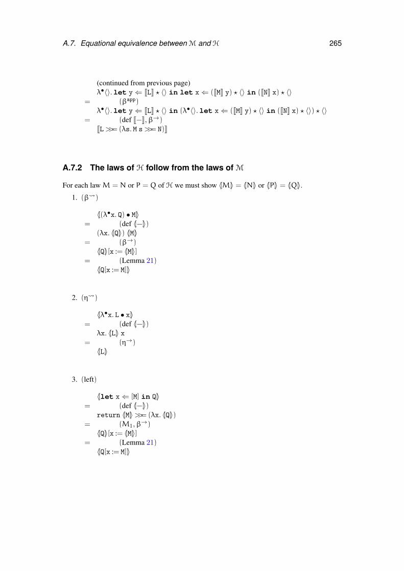
A.7. Equational equivalence between M and H 265
(continued from previous page)λ•〈〉.let y⇐ JLK ? 〈〉 in let x⇐ (JMK y) ? 〈〉 in (JNK x) ? 〈〉
= (βapp)λ•〈〉.let y⇐ JLK ? 〈〉 in (λ•〈〉.let x⇐ (JMK y) ? 〈〉 in (JNK x) ? 〈〉) ? 〈〉
= (def J−K,β→)JL>>= (λs. M s>>= N)K
A.7.2 The laws of H follow from the laws of M
For each lawM = N or P = Q of H we must show 〈[M]〉 = 〈[N]〉 or 〈[P]〉 = 〈[Q]〉.1. (β )
〈[(λ•x. Q) • M]〉= (def 〈[−]〉)
(λx. 〈[Q]〉) 〈[M]〉= (β→)〈[Q]〉[x := 〈[M]〉]
= (Lemma 21)〈[Q[x := M]]〉
2. (η )
〈[λ•x. L • x]〉= (def 〈[−]〉)
λx. 〈[L]〉 x= (η→)〈[L]〉
3. (left)
〈[let x⇐ [M] in Q]〉= (def 〈[−]〉)
return 〈[M]〉>>= (λx. 〈[Q]〉)= (M1,β→)〈[Q]〉[x := 〈[M]〉]
= (Lemma 21)〈[Q[x := M]]〉
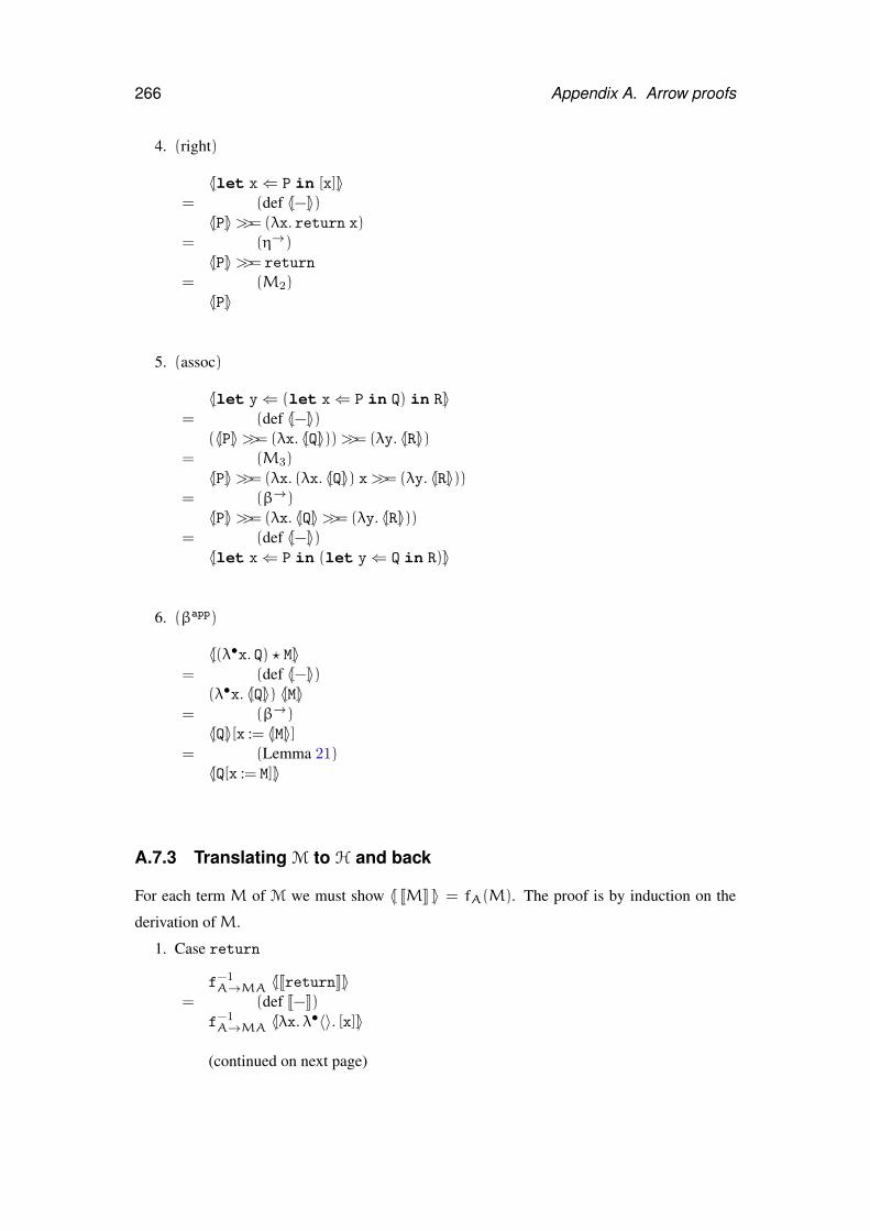
266 Appendix A. Arrow proofs
4. (right)
〈[let x⇐ P in [x]]〉= (def 〈[−]〉)〈[P]〉>>= (λx. return x)
= (η→)〈[P]〉>>= return
= (M2)〈[P]〉
5. (assoc)
〈[let y⇐ (let x⇐ P in Q) in R]〉= (def 〈[−]〉)
(〈[P]〉>>= (λx. 〈[Q]〉))>>= (λy. 〈[R]〉)= (M3)〈[P]〉>>= (λx. (λx. 〈[Q]〉) x>>= (λy. 〈[R]〉))
= (β→)〈[P]〉>>= (λx. 〈[Q]〉>>= (λy. 〈[R]〉))
= (def 〈[−]〉)〈[let x⇐ P in (let y⇐ Q in R)]〉
6. (βapp)
〈[(λ•x. Q) ? M]〉= (def 〈[−]〉)
(λ•x. 〈[Q]〉) 〈[M]〉= (β→)〈[Q]〉[x := 〈[M]〉]
= (Lemma 21)〈[Q[x := M]]〉
A.7.3 Translating M to H and back
For each term M of M we must show 〈[ JMK ]〉 = fA(M). The proof is by induction on the
derivation ofM.
1. Case return
f−1A→MA 〈[JreturnK]〉
= (def J−K)f−1A→MA 〈[λx. λ•〈〉. [x]]〉
(continued on next page)
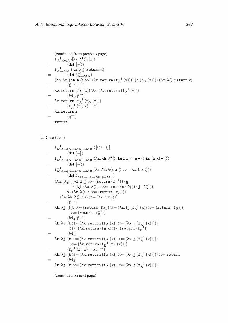
A.7. Equational equivalence between M and H 267
(continued from previous page)f−1A→MA 〈[λx. λ•〈〉. [x]]〉
= (def 〈[−]〉)f−1A→MA (λx. λ〈〉. return x)
= (def f−1A→MA)
(λh. λz. (λh. h 〈〉>>= (λv. return (f−1A (v)))) (h (fA (z)))) (λx. λ〈〉. return x)
= (β→,η→)
λz. return (fA (z))>>= (λv. return (f−1A (v)))
= (M1,β→)
λz. return (f−1A (fA (z)))
= (f−1A (fA x) = x)
λz. return z= (η→)
return
2. Case (>>=)
f−1MA→(A→MB)→MB 〈[J(>>=)K]〉
= (def J−K)f−1MA→(A→MB)→MB 〈[λa. λh. λ•〈〉.let x⇐ a • 〈〉 in (h x) • 〈〉]〉
= (def 〈[−]〉)f−1MA→(A→MB)→MB (λa. λh. λ〈〉. a 〈〉>>= (λx. h x 〈〉))
= (def f−1MA→(A→MB)→MB)
(λh. (λg. ((λl. l 〈〉>>= (return · f−1B )) · g
· (λj. (λa. λ〈〉. a>>= (return · fB)) · j · f−1A )))
· h · (λb. λ〈〉. b>>= (return · fA)))(λa. λh. λ〈〉. a 〈〉>>= (λx. h x 〈〉))
= (β→)
λb. λj. (((b>>= (return · fA))>>= (λx. (j (f−1A (x))>>= (return · fB))))
>>= (return · f−1B ))
= (M3,β→)
λb. λj. (b>>= (λx. return (fA (x))>>= (λx. j (f−1A (x)))))
>>= (λx. return (fB x)>>= (return · f−1B ))
= (M1)
λb. λj. (b>>= (λx. return (fA (x))>>= (λx. j (f−1A (x)))))
>>= (λx. return (f−1B (fB (x))))
= (f−1B (fB x) = x,η→)
λb. λj. (b>>= (λx. return (fA (x))>>= (λx. j (f−1A (x)))))>>= return
= (M2)
λb. λj. (b>>= (λx. return (fA (x))>>= (λx. j (f−1A (x)))))
(continued on next page)
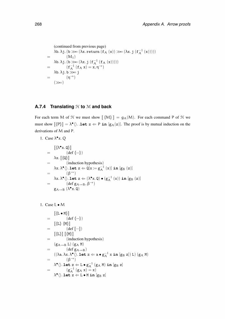
268 Appendix A. Arrow proofs
(continued from previous page)λb. λj. (b>>= (λx. return (fA (x))>>= (λx. j (f−1
A (x)))))= (M1)
λb. λj. (b>>= (λx. j (f−1A (fA (x)))))
= (f−1A (fA x) = x,η→)
λb. λj. b>>= j
= (η→)(>>=)
A.7.4 Translating H to M and back
For each term M of H we must show J 〈[M]〉 K = gA(M). For each command P of H we
must show J〈[P]〉K = λ•〈〉. .let z ⇐ P in [gA(z)]. The proof is by mutual induction on the
derivations ofM and P.
1. Case λ•x.Q
J〈[λ•x. Q]〉K= (def 〈[−]〉)
λx. J〈[Q]〉K= (induction hypothesis)
λx. λ•〈〉.let z⇐ Q[x := g−1A (x)] in [gB (z)]
= (β )
λx. λ•〈〉.let z⇐ (λ•x. Q) • (g−1A (x)) in [gB (z)]
= (def gA B,β→)gA B (λ•x. Q)
1. Case L •M
J〈[L • M]〉K= (def 〈[−]〉)
J〈[L]〉 〈[M]〉K= (def J−K)
J〈[L]〉K J〈[M]〉K= (induction hypothesis)
(gA B L) (gA M)= (def gA B)
((λa. λx. λ•〈〉.let z⇐ a • g−1A x in [gB z]) L) (gA M)
= (β→)
λ•〈〉.let z⇐ L • g−1A (gA M) in [gB z]
= (g−1A (gA x) = x)
λ•〈〉.let z⇐ L • M in [gB z]
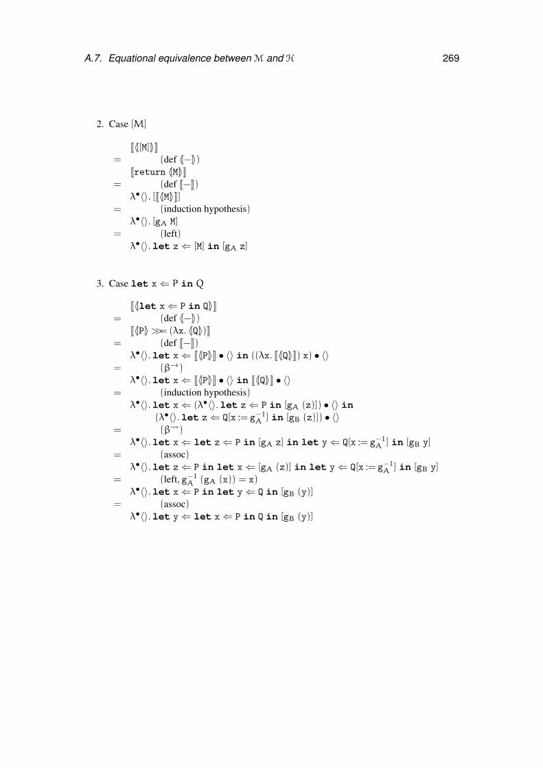
A.7. Equational equivalence between M and H 269
2. Case [M]
J〈[[M]]〉K= (def 〈[−]〉)
Jreturn 〈[M]〉K= (def J−K)
λ•〈〉. [J〈[M]〉K]= (induction hypothesis)
λ•〈〉. [gA M]= (left)
λ•〈〉.let z⇐ [M] in [gA z]
3. Case let x⇐ P in Q
J〈[let x⇐ P in Q]〉K= (def 〈[−]〉)
J〈[P]〉>>= (λx. 〈[Q]〉)K= (def J−K)
λ•〈〉.let x⇐ J〈[P]〉K • 〈〉 in ((λx. J〈[Q]〉K) x) • 〈〉= (β→)
λ•〈〉.let x⇐ J〈[P]〉K • 〈〉 in J〈[Q]〉K • 〈〉= (induction hypothesis)
λ•〈〉.let x⇐ (λ•〈〉.let z⇐ P in [gA (z)]) • 〈〉 in(λ•〈〉.let z⇐ Q[x := g−1
A ] in [gB (z)]) • 〈〉= (β )
λ•〈〉.let x⇐ let z⇐ P in [gA z] in let y⇐ Q[x := g−1A ] in [gB y]
= (assoc)λ•〈〉.let z⇐ P in let x⇐ [gA (z)] in let y⇐ Q[x := g−1
A ] in [gB y]
= (left, g−1A (gA (x)) = x)
λ•〈〉.let x⇐ P in let y⇐ Q in [gB (y)]= (assoc)
λ•〈〉.let y⇐ let x⇐ P in Q in [gB (y)]
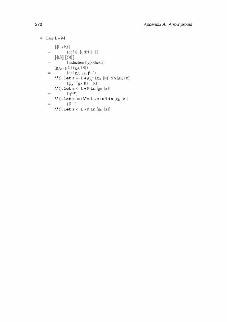
270 Appendix A. Arrow proofs
4. Case L ?M
J〈[L ? M]〉K= (def 〈[−]〉, def J−K)
J〈[L]〉K J〈[M]〉K= (induction hypothesis)
(gA B L) (gA (M))= (def gA B,β→)
λ•〈〉.let z⇐ L • g−1A (gA (M)) in [gB (z)]
= (g−1A (gA M) = M)
λ•〈〉.let z⇐ L • M in [gB (z)]= (ηapp)
λ•〈〉.let z⇐ (λ•x. L ? x) • M in [gB (z)]= (β )
λ•〈〉.let z⇐ L ? M in [gB (z)]
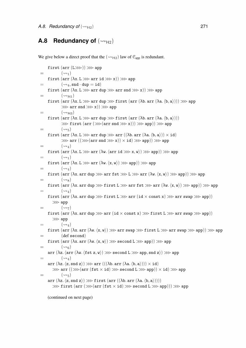
A.8. Redundancy of ( H2) 271
A.8 Redundancy of ( H2)
We give below a direct proof that the ( H2) law of Capp is redundant.
first (arr (L>>>))>>> app
= ( 1)first (arr (λx. L>>> arr id>>> x))>>> app
= ( 4, snd · dup = id)first (arr (λx. L>>> arr dup>>> arr snd>>> x))>>> app
= ( H1)first (arr (λx. L>>> arr dup>>> first (arr (λb. arr (λa. 〈b, a〉)))>>> app
>>> arr snd>>> x))>>> app
= ( H3)first (arr (λx. L>>> arr dup>>> first (arr (λb. arr (λa. 〈b, a〉)))
>>> first (arr (>>>(arr snd>>> x)))>>> app))>>> app
= ( 5)first (arr (λx. L>>> arr dup>>> arr ((λb. arr (λa. 〈b, a〉))× id)
>>> arr ((>>>(arr snd>>> x))× id)>>> app))>>> app
= ( 4)first (arr (λx. L>>> arr (λw. 〈arr id>>> x, w〉)>>> app))>>> app
= ( 1)first (arr (λx. L>>> arr (λw. 〈x, w〉)>>> app))>>> app
= ( 4)first (arr (λx. arr dup>>> arr fst>>> L>>> arr (λw. 〈x, w〉)>>> app))>>> app
= ( 8)first (arr (λx. arr dup>>> first L>>> arr fst>>> arr (λw. 〈x, w〉)>>> app))>>> app
= ( 4)first (arr (λx. arr dup>>> first L>>> arr (id× const x)>>> arr swap>>> app))>>> app
= ( 7)first (arr (λx. arr dup>>> arr (id× const x)>>> first L>>> arr swap>>> app))>>> app
= ( 4)first (arr (λx. arr (λw. 〈x, w〉)>>> arr swap>>> first L>>> arr swap>>> app))>>> app
= (def second)first (arr (λx. arr (λw. 〈x, w〉)>>> second L>>> app))>>> app
= ( 6)arr (λz. 〈arr (λw. 〈fst z, w〉)>>> second L>>> app, snd z〉)>>> app
= ( 4)arr (λz. 〈z, snd z〉)>>> arr (((λb. arr (λa. 〈b, a〉)))× id)>>> arr ((>>>(arr (fst× id)>>> second L>>> app))× id)>>> app
= ( 5)arr (λz. 〈z, snd z〉)>>> first (arr ((λb. arr (λa. 〈b, a〉))))>>> first (arr (>>>(arr (fst× id)>>> second L>>> app)))>>> app
(continued on next page)
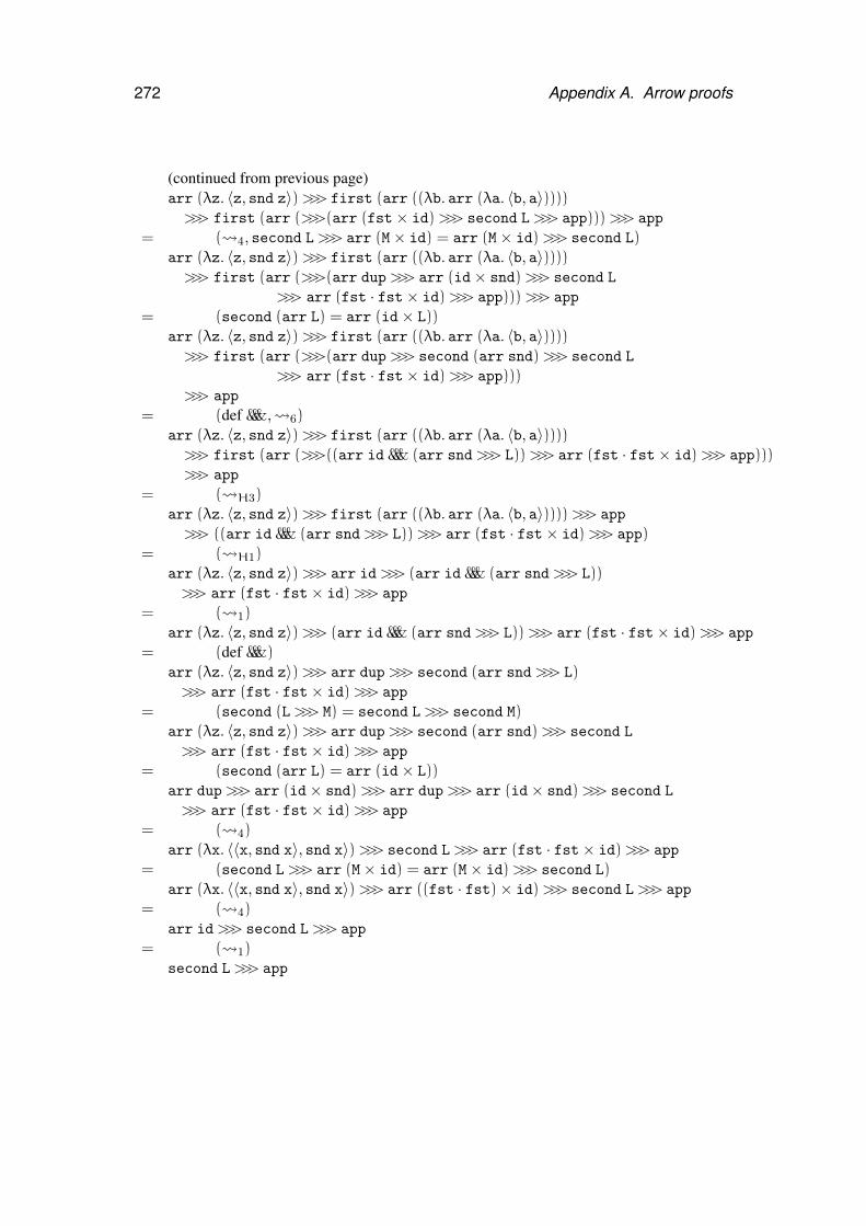
272 Appendix A. Arrow proofs
(continued from previous page)arr (λz. 〈z, snd z〉)>>> first (arr ((λb. arr (λa. 〈b, a〉))))>>> first (arr (>>>(arr (fst× id)>>> second L>>> app)))>>> app
= ( 4, second L>>> arr (M× id) = arr (M× id)>>> second L)arr (λz. 〈z, snd z〉)>>> first (arr ((λb. arr (λa. 〈b, a〉))))>>> first (arr (>>>(arr dup>>> arr (id× snd)>>> second L
>>> arr (fst · fst× id)>>> app)))>>> app
= (second (arr L) = arr (id× L))arr (λz. 〈z, snd z〉)>>> first (arr ((λb. arr (λa. 〈b, a〉))))>>> first (arr (>>>(arr dup>>> second (arr snd)>>> second L
>>> arr (fst · fst× id)>>> app)))>>> app
= (def &&&, 6)arr (λz. 〈z, snd z〉)>>> first (arr ((λb. arr (λa. 〈b, a〉))))>>> first (arr (>>>((arr id &&& (arr snd>>> L))>>> arr (fst · fst× id)>>> app)))>>> app
= ( H3)arr (λz. 〈z, snd z〉)>>> first (arr ((λb. arr (λa. 〈b, a〉))))>>> app
>>> ((arr id &&& (arr snd>>> L))>>> arr (fst · fst× id)>>> app)= ( H1)
arr (λz. 〈z, snd z〉)>>> arr id>>> (arr id &&& (arr snd>>> L))>>> arr (fst · fst× id)>>> app
= ( 1)arr (λz. 〈z, snd z〉)>>> (arr id &&& (arr snd>>> L))>>> arr (fst · fst× id)>>> app
= (def &&&)arr (λz. 〈z, snd z〉)>>> arr dup>>> second (arr snd>>> L)>>> arr (fst · fst× id)>>> app
= (second (L>>> M) = second L>>> second M)arr (λz. 〈z, snd z〉)>>> arr dup>>> second (arr snd)>>> second L
>>> arr (fst · fst× id)>>> app
= (second (arr L) = arr (id× L))arr dup>>> arr (id× snd)>>> arr dup>>> arr (id× snd)>>> second L
>>> arr (fst · fst× id)>>> app
= ( 4)arr (λx. 〈〈x, snd x〉, snd x〉)>>> second L>>> arr (fst · fst× id)>>> app
= (second L>>> arr (M× id) = arr (M× id)>>> second L)arr (λx. 〈〈x, snd x〉, snd x〉)>>> arr ((fst · fst)× id)>>> second L>>> app
= ( 4)arr id>>> second L>>> app
= ( 1)second L>>> app
Appendix B
Formlets extras
B.1 The page construct
This appendix describes the page construct, which is used in combination with input-validating
formlets (Section 3.6.2). The function of the page construct is to associate the context in which
each formlet appears with the value representing the formlet. If the input submitted by the user
is determined to be invalid, the formlet then re-renders itself together in the context, together
with error messages indicating the problems wit the input.
The page construct really represents composable page fragments, just as formlets rep-
resent fragments of forms. As with formlets, we provide a new syntactic form based on
XML literals with embedded expressions. Consider the date example of Figure 3.1. The fi-
nal step in that example is to associate the formlet travel_formlet with the continuation
display_itinerary:
handle travel_formlet display_itinerary
The page construct subsumes the functionality of handle: it associates a formlet with its con-
tinuation in the context of some larger XML value. For example, the following code associates
travel_formlet with display_itinerary in the context of the enclosing <body> ele-
ment.
page<body
<h1>Itinerary</h1>{travel_formlet =⇒ display_itinerary}
</body>
As we have said, the page construct is designed for use with input-validating formlets, where
there are two possible outcomes when a form is submitted. Suppose that travel_formlet
273
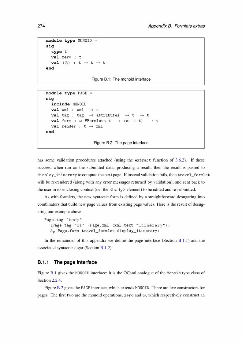
274 Appendix B. Formlets extras
module type MONOID =sigtype t
val zero : t
val (⊗) : t → t → t
end
Figure B.1: The monoid interface
module type PAGE =siginclude MONOID
val xml : xml → t
val tag : tag → attributes → t → t
val form : α VFormlets.t → (α → t) → t
val render : t → xml
end
Figure B.2: The page interface
has some validation procedures attached (using the extract function of 3.6.2). If these
succeed when run on the submitted data, producing a result, then the result is passed to
display_itinerary to compute the next page. If instead validation fails, then travel_formlet
will be re-rendered (along with any error messages returned by validation), and sent back to
the user in its enclosing context (i.e. the <body> element) to be edited and re-submitted.
As with formlets, the new syntactic form is defined by a straightforward desugaring into
combinators that build new page values from existing page values. Here is the result of desug-
aring our example above:
Page.tag "body"(Page.tag "h1" (Page.xml (xml_text "Itinerary"))⊗p Page.form travel_formlet display_itinerary)
In the remainder of this appendix we define the page interface (Section B.1.1) and the
associated syntactic sugar (Section B.1.2).
B.1.1 The page interface
Figure B.1 gives the MONOID interface; it is the OCaml analogue of the Monoid type class of
Section 2.2.4.
Figure B.2 gives the PAGE interface, which extends MONOID. There are five constructors for
pages. The first two are the monoid operations, zero and ⊗, which respectively construct an
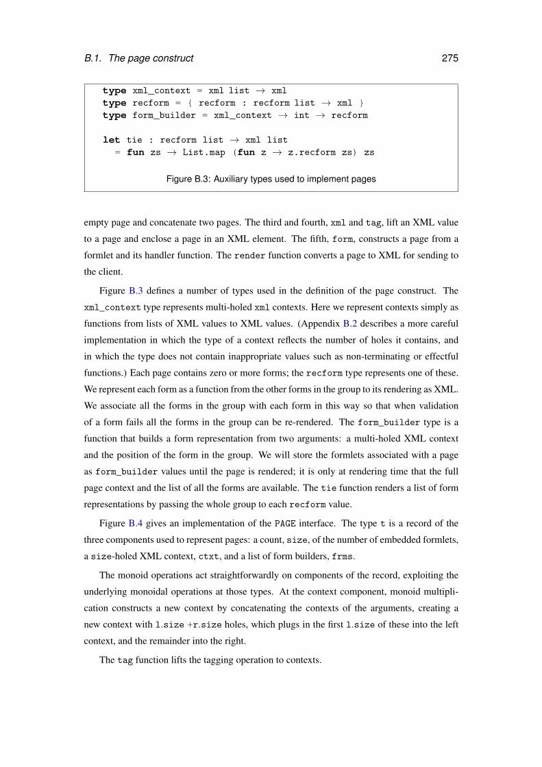
B.1. The page construct 275
type xml_context = xml list → xml
type recform = { recform : recform list → xml }type form_builder = xml_context → int → recform
let tie : recform list → xml list
= fun zs → List.map (fun z → z.recform zs) zs
Figure B.3: Auxiliary types used to implement pages
empty page and concatenate two pages. The third and fourth, xml and tag, lift an XML value
to a page and enclose a page in an XML element. The fifth, form, constructs a page from a
formlet and its handler function. The render function converts a page to XML for sending to
the client.
Figure B.3 defines a number of types used in the definition of the page construct. The
xml_context type represents multi-holed xml contexts. Here we represent contexts simply as
functions from lists of XML values to XML values. (Appendix B.2 describes a more careful
implementation in which the type of a context reflects the number of holes it contains, and
in which the type does not contain inappropriate values such as non-terminating or effectful
functions.) Each page contains zero or more forms; the recform type represents one of these.
We represent each form as a function from the other forms in the group to its rendering as XML.
We associate all the forms in the group with each form in this way so that when validation
of a form fails all the forms in the group can be re-rendered. The form_builder type is a
function that builds a form representation from two arguments: a multi-holed XML context
and the position of the form in the group. We will store the formlets associated with a page
as form_builder values until the page is rendered; it is only at rendering time that the full
page context and the list of all the forms are available. The tie function renders a list of form
representations by passing the whole group to each recform value.
Figure B.4 gives an implementation of the PAGE interface. The type t is a record of the
three components used to represent pages: a count, size, of the number of embedded formlets,
a size-holed XML context, ctxt, and a list of form builders, frms.
The monoid operations act straightforwardly on components of the record, exploiting the
underlying monoidal operations at those types. At the context component, monoid multipli-
cation constructs a new context by concatenating the contexts of the arguments, creating a
new context with l.size +r.size holes, which plugs in the first l.size of these into the left
context, and the remainder into the right.
The tag function lifts the tagging operation to contexts.
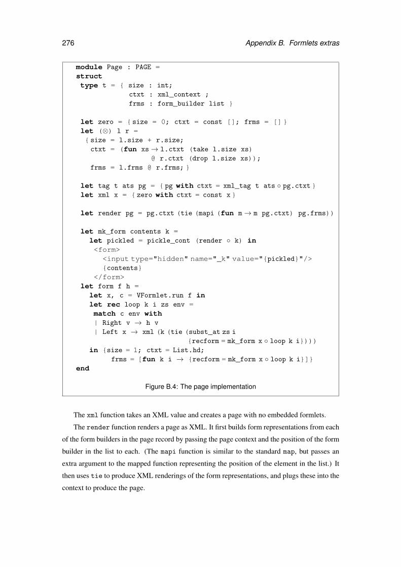
276 Appendix B. Formlets extras
module Page : PAGE =structtype t = { size : int;
ctxt : xml_context ;frms : form_builder list }
let zero = { size = 0; ctxt = const []; frms = []}let (⊗) l r ={ size = l.size + r.size;ctxt = (fun xs→ l.ctxt (take l.size xs)
@ r.ctxt (drop l.size xs));frms = l.frms @ r.frms;}
let tag t ats pg = { pg with ctxt = xml_tag t ats ◦ pg.ctxt}let xml x = { zero with ctxt = const x}
let render pg = pg.ctxt (tie (mapi (fun m→ m pg.ctxt) pg.frms))
let mk_form contents k =let pickled = pickle_cont (render ◦ k) in<form>
<input type="hidden" name="_k" value="{pickled}"/>{contents}
</form>let form f h =let x, c = VFormlet.run f inlet rec loop k i zs env =match c env with| Right v → h v
| Left x → xml (k (tie (subst_at zs i
{recform = mk_form x ◦ loop k i})))in {size = 1; ctxt = List.hd;
frms = [fun k i → {recform = mk_form x ◦ loop k i}]}end
Figure B.4: The page implementation
The xml function takes an XML value and creates a page with no embedded formlets.
The render function renders a page as XML. It first builds form representations from each
of the form builders in the page record by passing the page context and the position of the form
builder in the list to each. (The mapi function is similar to the standard map, but passes an
extra argument to the mapped function representing the position of the element in the list.) It
then uses tie to produce XML renderings of the form representations, and plugs these into the
context to produce the page.
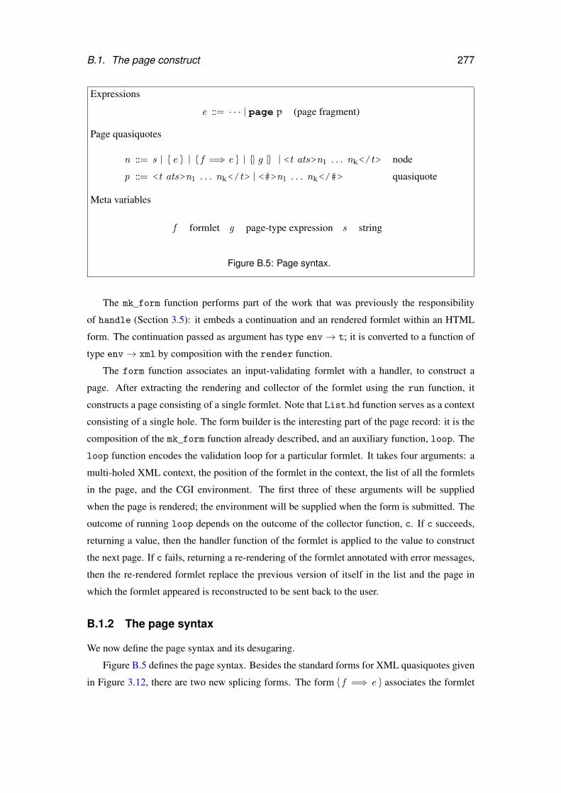
B.1. The page construct 277
Expressions
e ::= · · · | page p (page fragment)
Page quasiquotes
n ::= s | { e } | { f =⇒ e } | {| g |} | <t ats>n1 . . . nk</t> node
p ::= <t ats>n1 . . . nk</t> | <#>n1 . . . nk</#> quasiquote
Meta variables
f formlet g page-type expression s string
Figure B.5: Page syntax.
The mk_form function performs part of the work that was previously the responsibility
of handle (Section 3.5): it embeds a continuation and an rendered formlet within an HTML
form. The continuation passed as argument has type env→ t; it is converted to a function of
type env→ xml by composition with the render function.
The form function associates an input-validating formlet with a handler, to construct a
page. After extracting the rendering and collector of the formlet using the run function, it
constructs a page consisting of a single formlet. Note that List.hd function serves as a context
consisting of a single hole. The form builder is the interesting part of the page record: it is the
composition of the mk_form function already described, and an auxiliary function, loop. The
loop function encodes the validation loop for a particular formlet. It takes four arguments: a
multi-holed XML context, the position of the formlet in the context, the list of all the formlets
in the page, and the CGI environment. The first three of these arguments will be supplied
when the page is rendered; the environment will be supplied when the form is submitted. The
outcome of running loop depends on the outcome of the collector function, c. If c succeeds,
returning a value, then the handler function of the formlet is applied to the value to construct
the next page. If c fails, returning a re-rendering of the formlet annotated with error messages,
then the re-rendered formlet replace the previous version of itself in the list and the page in
which the formlet appeared is reconstructed to be sent back to the user.
B.1.2 The page syntax
We now define the page syntax and its desugaring.
Figure B.5 defines the page syntax. Besides the standard forms for XML quasiquotes given
in Figure 3.12, there are two new splicing forms. The form { f =⇒ e } associates the formlet
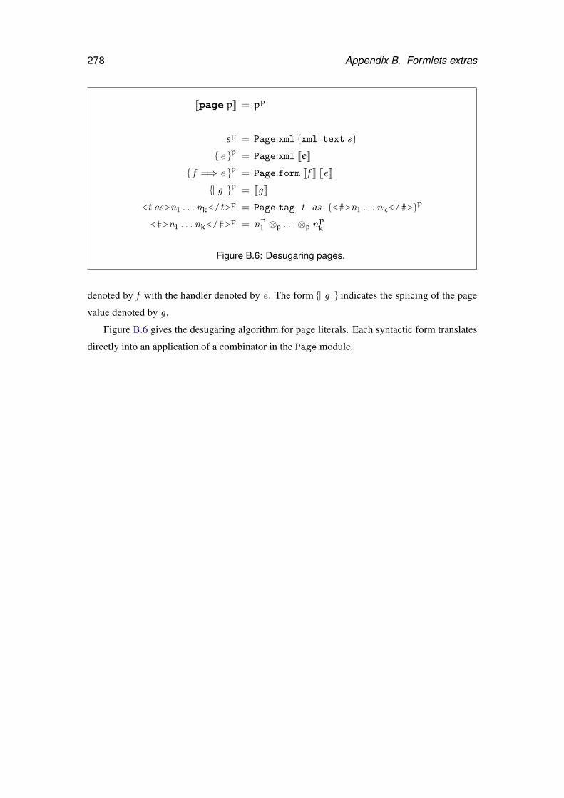
278 Appendix B. Formlets extras
Jpage pK = pp
sp = Page.xml (xml_text s)
{ e }p = Page.xml JeK
{ f =⇒ e }p = Page.form Jf K JeK
{| g |}p = JgK
<t as>n1 . . .nk</t>p = Page.tag t as (<#>n1 . . .nk</#>)p
<#>n1 . . .nk</#>p = np1 ⊗p . . .⊗p npk
Figure B.6: Desugaring pages.
denoted by f with the handler denoted by e . The form {| g |} indicates the splicing of the page
value denoted by g .
Figure B.6 gives the desugaring algorithm for page literals. Each syntactic form translates
directly into an application of a combinator in the Page module.
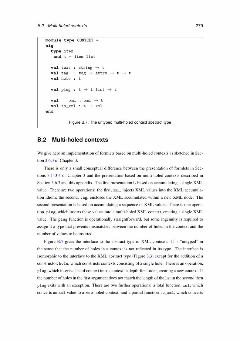
B.2. Multi-holed contexts 279
module type CONTEXT =sig
type item
and t = item list
val text : string → t
val tag : tag → attrs → t → t
val hole : t
val plug : t → t list → t
val xml : xml → t
val to_xml : t → xml
end
Figure B.7: The untyped multi-holed context abstract type
B.2 Multi-holed contexts
We give here an implementation of formlets based on multi-holed contexts as sketched in Sec-
tion 3.6.3 of Chapter 3.
There is only a small conceptual difference between the presentation of formlets in Sec-
tions 3.1–3.4 of Chapter 3 and the presentation based on multi-holed contexts described in
Section 3.6.3 and this appendix. The first presentation is based on accumulating a single XML
value. There are two operations: the first, xml, injects XML values into the XML accumula-
tion idiom; the second, tag, encloses the XML accumulated within a new XML node. The
second presentation is based on accumulating a sequence of XML values. There is one opera-
tion, plug, which inserts these values into a multi-holed XML context, creating a single XML
value. The plug function is operationally straightforward, but some ingenuity is required to
assign it a type that prevents mismatches between the number of holes in the context and the
number of values to be inserted.
Figure B.7 gives the interface to the abstract type of XML contexts. It is “untyped” in
the sense that the number of holes in a context is not reflected in its type. The interface is
isomorphic to the interface to the XML abstract type (Figure 3.3) except for the addition of a
constructor, hole, which constructs contexts consisting of a single hole. There is an operation,
plug, which inserts a list of context into a context in depth-first order, creating a new context. If
the number of holes in the first argument does not match the length of the list in the second then
plug exits with an exception. There are two further operations: a total function, xml, which
converts an xml value to a zero-holed context, and a partial function to_xml, which converts
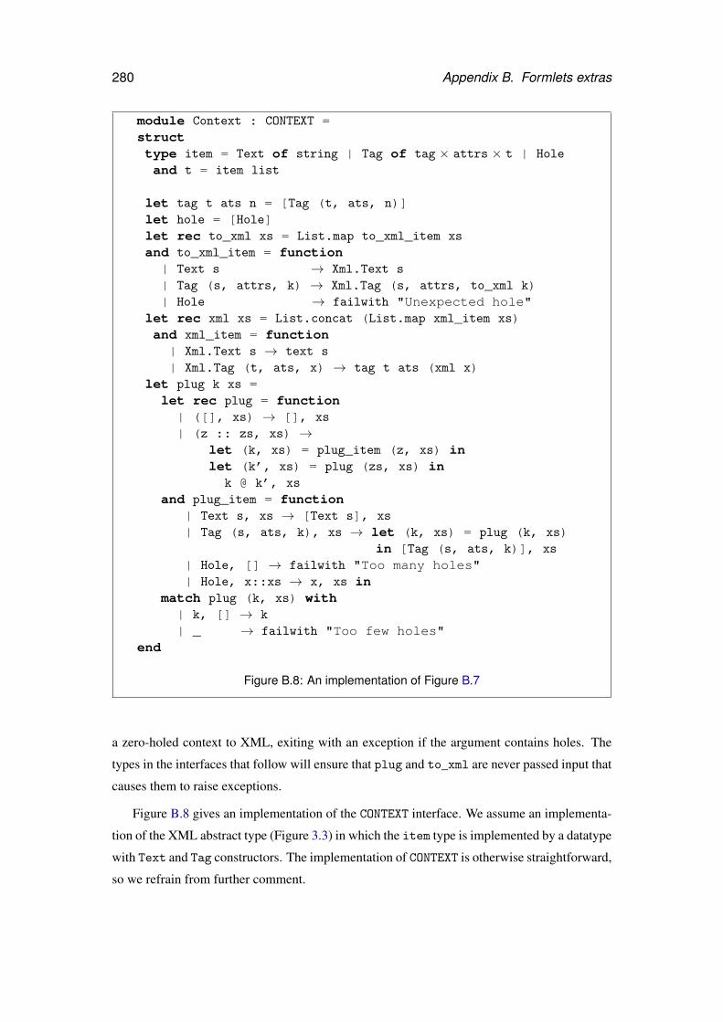
280 Appendix B. Formlets extras
module Context : CONTEXT =structtype item = Text of string | Tag of tag × attrs × t | Hole
and t = item list
let tag t ats n = [Tag (t, ats, n)]let hole = [Hole]let rec to_xml xs = List.map to_xml_item xs
and to_xml_item = function| Text s → Xml.Text s
| Tag (s, attrs, k) → Xml.Tag (s, attrs, to_xml k)| Hole → failwith "Unexpected hole"
let rec xml xs = List.concat (List.map xml_item xs)and xml_item = function| Xml.Text s → text s
| Xml.Tag (t, ats, x) → tag t ats (xml x)let plug k xs =
let rec plug = function| ([], xs) → [], xs
| (z :: zs, xs) →let (k, xs) = plug_item (z, xs) inlet (k’, xs) = plug (zs, xs) in
k @ k’, xs
and plug_item = function| Text s, xs → [Text s], xs
| Tag (s, ats, k), xs → let (k, xs) = plug (k, xs)in [Tag (s, ats, k)], xs
| Hole, [] → failwith "Too many holes"| Hole, x::xs → x, xs in
match plug (k, xs) with| k, [] → k
| _ → failwith "Too few holes"end
Figure B.8: An implementation of Figure B.7
a zero-holed context to XML, exiting with an exception if the argument contains holes. The
types in the interfaces that follow will ensure that plug and to_xml are never passed input that
causes them to raise exceptions.
Figure B.8 gives an implementation of the CONTEXT interface. We assume an implementa-
tion of the XML abstract type (Figure 3.3) in which the item type is implemented by a datatype
with Text and Tag constructors. The implementation of CONTEXT is otherwise straightforward,
so we refrain from further comment.
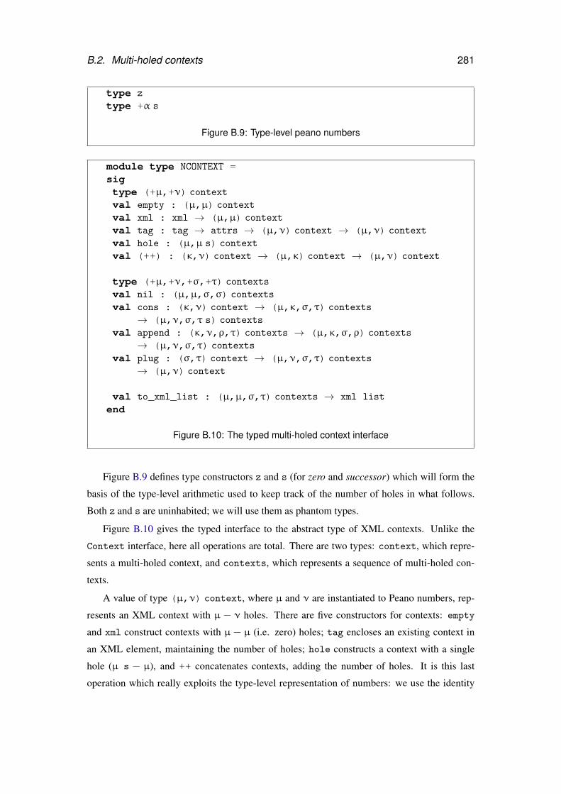
B.2. Multi-holed contexts 281
type z
type +α s
Figure B.9: Type-level peano numbers
module type NCONTEXT =sigtype (+µ,+ν) context
val empty : (µ,µ) context
val xml : xml → (µ,µ) context
val tag : tag → attrs → (µ,ν) context → (µ,ν) context
val hole : (µ,µ s) context
val (++) : (κ,ν) context → (µ,κ) context → (µ,ν) context
type (+µ,+ν,+σ,+τ) contexts
val nil : (µ,µ,σ,σ) contexts
val cons : (κ,ν) context → (µ,κ,σ,τ) contexts
→ (µ,ν,σ,τ s) contexts
val append : (κ,ν,ρ,τ) contexts → (µ,κ,σ,ρ) contexts
→ (µ,ν,σ,τ) contexts
val plug : (σ,τ) context → (µ,ν,σ,τ) contexts
→ (µ,ν) context
val to_xml_list : (µ,µ,σ,τ) contexts → xml list
end
Figure B.10: The typed multi-holed context interface
Figure B.9 defines type constructors z and s (for zero and successor) which will form the
basis of the type-level arithmetic used to keep track of the number of holes in what follows.
Both z and s are uninhabited; we will use them as phantom types.
Figure B.10 gives the typed interface to the abstract type of XML contexts. Unlike the
Context interface, here all operations are total. There are two types: context, which repre-
sents a multi-holed context, and contexts, which represents a sequence of multi-holed con-
texts.
A value of type (µ,ν) context, where µ and ν are instantiated to Peano numbers, rep-
resents an XML context with µ − ν holes. There are five constructors for contexts: empty
and xml construct contexts with µ − µ (i.e. zero) holes; tag encloses an existing context in
an XML element, maintaining the number of holes; hole constructs a context with a single
hole (µ s − µ), and ++ concatenates contexts, adding the number of holes. It is this last
operation which really exploits the type-level representation of numbers: we use the identity
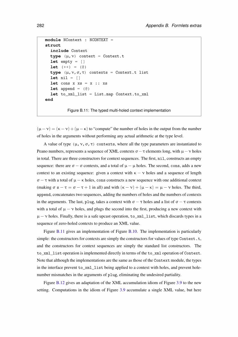
282 Appendix B. Formlets extras
module NContext : NCONTEXT =struct
include Context
type (µ,ν) context = Context.tlet empty = []let (++) = (@)type (µ,ν,σ,τ) contexts = Context.t list
let nil = []let cons x xs = x :: xs
let append = (@)let to_xml_list = List.map Context.to_xml
end
Figure B.11: The typed multi-holed context implementation
(µ− ν) = (κ− ν) + (µ− κ) to “compute” the number of holes in the output from the number
of holes in the arguments without performing any actual arithmetic at the type level.
A value of type (µ,ν,σ,τ) contexts, where all the type parameters are instantiated to
Peano numbers, represents a sequence of XML contexts σ− τ elements long, with µ−ν holes
in total. There are three constructors for context sequences. The first, nil, constructs an empty
sequence: there are σ − σ contexts, and a total of µ − µ holes. The second, cons, adds a new
context to an existing sequence: given a context with κ − ν holes and a sequence of length
σ− τ with a total of µ− κ holes, cons constructs a new sequence with one additional context
(making σ s − τ = σ − τ + 1 in all) and with (κ − ν) + (µ − κ) = µ − ν holes. The third,
append, concatenates two sequences, adding the numbers of holes and the numbers of contexts
in the arguments. The last, plug, takes a context with σ − τ holes and a list of σ − τ contexts
with a total of µ − ν holes, and plugs the second into the first, producing a new context with
µ− ν holes. Finally, there is a safe upcast operation, to_xml_list, which discards types in a
sequence of zero-holed contexts to produce an XML value.
Figure B.11 gives an implementation of Figure B.10. The implementation is particularly
simple: the constructors for contexts are simply the constructors for values of type Context.t,
and the constructors for context sequences are simply the standard list constructors. The
to_xml_list operation is implemented directly in terms of the to_xml operation of Context.
Note that although the implementations are the same as those of the Context module, the types
in the interface prevent to_xml_list being applied to a context with holes, and prevent hole-
number mismatches in the arguments of plug, eliminating the undesired partiality.
Figure B.12 gives an adaptation of the XML accumulation idiom of Figure 3.9 to the new
setting. Computations in the idiom of Figure 3.9 accumulate a single XML value, but here
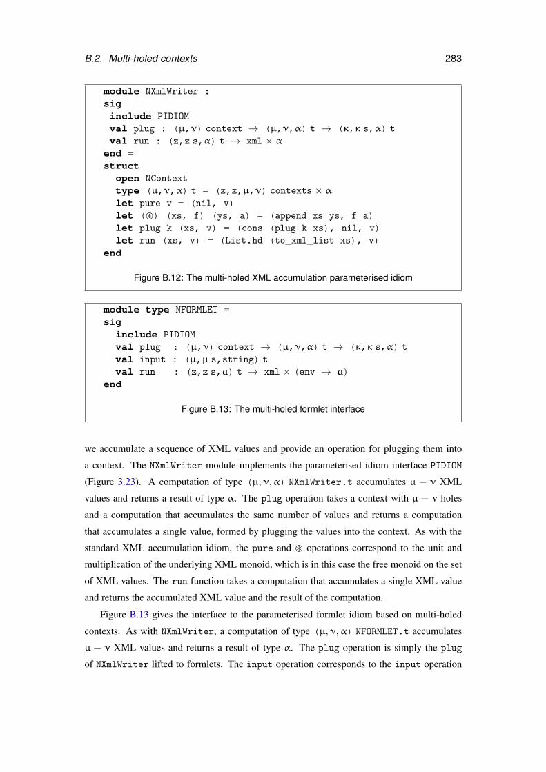
B.2. Multi-holed contexts 283
module NXmlWriter :siginclude PIDIOM
val plug : (µ,ν) context → (µ,ν,α) t → (κ,κ s,α) t
val run : (z,z s,α) t → xml × αend =struct
open NContext
type (µ,ν,α) t = (z,z,µ,ν) contexts × αlet pure v = (nil, v)let (�) (xs, f) (ys, a) = (append xs ys, f a)let plug k (xs, v) = (cons (plug k xs), nil, v)let run (xs, v) = (List.hd (to_xml_list xs), v)
end
Figure B.12: The multi-holed XML accumulation parameterised idiom
module type NFORMLET =sig
include PIDIOM
val plug : (µ,ν) context → (µ,ν,α) t → (κ,κ s,α) t
val input : (µ,µ s,string) t
val run : (z,z s,a) t → xml × (env → a)end
Figure B.13: The multi-holed formlet interface
we accumulate a sequence of XML values and provide an operation for plugging them into
a context. The NXmlWriter module implements the parameterised idiom interface PIDIOM
(Figure 3.23). A computation of type (µ,ν,α) NXmlWriter.t accumulates µ − ν XML
values and returns a result of type α. The plug operation takes a context with µ − ν holes
and a computation that accumulates the same number of values and returns a computation
that accumulates a single value, formed by plugging the values into the context. As with the
standard XML accumulation idiom, the pure and � operations correspond to the unit and
multiplication of the underlying XML monoid, which is in this case the free monoid on the set
of XML values. The run function takes a computation that accumulates a single XML value
and returns the accumulated XML value and the result of the computation.
Figure B.13 gives the interface to the parameterised formlet idiom based on multi-holed
contexts. As with NXmlWriter, a computation of type (µ,ν,α) NFORMLET.t accumulates
µ − ν XML values and returns a result of type α. The plug operation is simply the plug
of NXmlWriter lifted to formlets. The input operation corresponds to the input operation
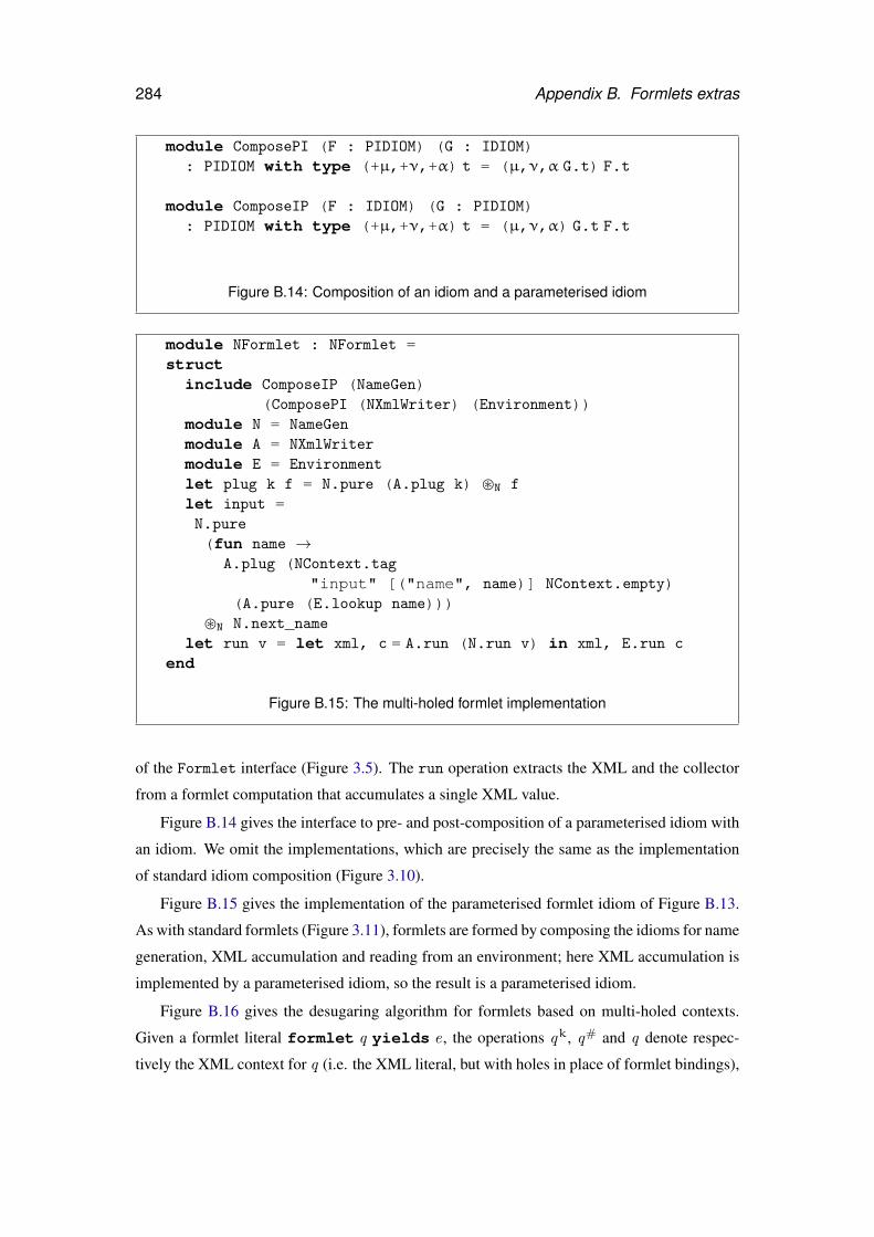
284 Appendix B. Formlets extras
module ComposePI (F : PIDIOM) (G : IDIOM): PIDIOM with type (+µ,+ν,+α) t = (µ,ν,α G.t) F.t
module ComposeIP (F : IDIOM) (G : PIDIOM): PIDIOM with type (+µ,+ν,+α) t = (µ,ν,α) G.t F.t
Figure B.14: Composition of an idiom and a parameterised idiom
module NFormlet : NFormlet =struct
include ComposeIP (NameGen)(ComposePI (NXmlWriter) (Environment))
module N = NameGen
module A = NXmlWriter
module E = Environment
let plug k f = N.pure (A.plug k) �N f
let input =N.pure(fun name →
A.plug (NContext.tag"input" [("name", name)] NContext.empty)
(A.pure (E.lookup name)))�N N.next_name
let run v = let xml, c = A.run (N.run v) in xml, E.run c
end
Figure B.15: The multi-holed formlet implementation
of the Formlet interface (Figure 3.5). The run operation extracts the XML and the collector
from a formlet computation that accumulates a single XML value.
Figure B.14 gives the interface to pre- and post-composition of a parameterised idiom with
an idiom. We omit the implementations, which are precisely the same as the implementation
of standard idiom composition (Figure 3.10).
Figure B.15 gives the implementation of the parameterised formlet idiom of Figure B.13.
As with standard formlets (Figure 3.11), formlets are formed by composing the idioms for name
generation, XML accumulation and reading from an environment; here XML accumulation is
implemented by a parameterised idiom, so the result is a parameterised idiom.
Figure B.16 gives the desugaring algorithm for formlets based on multi-holed contexts.
Given a formlet literal formlet q yields e , the operations qk, q# and q denote respec-
tively the XML context for q (i.e. the XML literal, but with holes in place of formlet bindings),
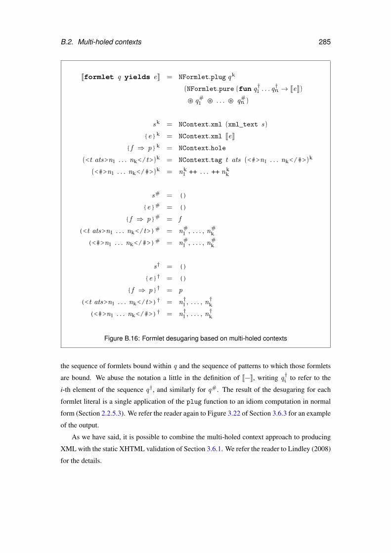
B.2. Multi-holed contexts 285
Jformlet q yields eK = NFormlet.plug qk
(NFormlet.pure (fun q†1 . . . q†n → JeK)
� q#1 � . . . � q#
n )
sk = NContext.xml (xml_text s)
{e}k = NContext.xml JeK
{f ⇒ p}k = NContext.hole
(<t ats>n1 . . . nk</t>)k = NContext.tag t ats (<#>n1 . . . nk</#>)k
(<#>n1 . . . nk</#>)k = nk1 ++ . . . ++ nkk
s# = ()
{e}# = ()
{f ⇒ p}# = f
(<t ats>n1 . . . nk</t>)# = n#1 , . . . , n#
k
(<#>n1 . . . nk</#>)# = n#1 , . . . , n#
k
s† = ()
{e}† = ()
{f ⇒ p}† = p
(<t ats>n1 . . . nk</t>)† = n†1 , . . . , n†k
(<#>n1 . . . nk</#>)† = n†1 , . . . , n†k
Figure B.16: Formlet desugaring based on multi-holed contexts
the sequence of formlets bound within q and the sequence of patterns to which those formlets
are bound. We abuse the notation a little in the definition of J−K, writing q†i to refer to the
i-th element of the sequence q†, and similarly for q#. The result of the desugaring for each
formlet literal is a single application of the plug function to an idiom computation in normal
form (Section 2.2.5.3). We refer the reader again to Figure 3.22 of Section 3.6.3 for an example
of the output.
As we have said, it is possible to combine the multi-holed context approach to producing
XML with the static XHTML validation of Section 3.6.1. We refer the reader to Lindley (2008)
for the details.

Bibliography
RFC 793, 1981. Transmission Control Protocol
http://tools.ietf.org/html/rfc793.
Lift website, March 2008.
http://liftweb.net/.
Martín Abadi. Access control in a core calculus of dependency. Electronic Notes in Theoretical
Computer Science, 172:5–31, 2007. ISSN 1571-0661.
Andrew W. Appel. Compiling with Continuations. Cambridge University Press, New York,
NY, USA, 2007.
Robert Atkey. What is a categorical model of arrows? In Venanzio Capretta and Conor
McBride, editors, Mathematically Structured Functional Programming, Reykjavik Univer-
sity, Iceland, July 2008.
Robert Atkey. Parameterised notions of computation. Journal of Functional Programming, 19
(3 & 4):355–376, July 2009.
Vincent Balat. Ocsigen: typing web interaction with Objective Caml. In ACM SIGPLAN
Workshop on ML, pages 84–94, Portland, Oregon, September 2006.
Ioannis G. Baltopoulos and Andrew D. Gordon. Secure compilation of a multi-tier web lan-
guage. In ACM SIGPLAN Workshop on Types in Language Design and Implementation,
pages 27–38, Savannah, GA, USA, January 2009. ISBN 978-1-60558-420-1.
John Billings, Peter Sewell, Mark Shinwell, and Rok Strniša. Type-safe distributed program-
ming for OCaml. In ACM SIGPLAN Workshop on ML, Portland, Oregon, September 2006.
Richard Bird. A program to solve sudoku. Journal of Functional Programming, 16(6):671–
679, July 2006.
287
288 Bibliography
Claus Brabrand, Anders Møller, and Michael I. Schwartzbach. Static validation of dynami-
cally generated HTML. In ACM SIGPLAN-SIGSOFT Workshop on Program Analysis For
Software Tools and Engineering, pages 38–45, Snowbird, Utah, USA, June 2001.
Björn Bringert and Aarne Ranta. A pattern for almost compositional functions. In ACM
SIGPLAN International Conference on Functional Programming, Portland, Oregon, USA,
September 2006.
Manuel M. T. Chakravarty, Gabriele Keller, and Simon Peyton Jones. Associated type syn-
onyms. In ACM SIGPLAN International Conference on Functional Programming, pages
241–253, Tallinn, Estonia, September 2005a.
Manuel M. T. Chakravarty, Gabriele Keller, Simon Peyton Jones, and Simon Marlow. Associ-
ated types with class. In ACM SIGPLAN-SIGACT Symposium on Principles of Programming
Languages, pages 1–13, Long Beach, California, USA, January 2005b.
James Cheney and Ralf Hinze. A lightweight implementation of generics and dynamics. In
ACM SIGPLAN Haskell Workshop, Pittsburgh, PA, USA, October 2002.
Noam Chomsky. Three models for the description of language. IRE Transactions on Informa-
tion Theory, (2):113–124, 1956.
Aske Simon Christensen, Anders Møller, and Michael I. Schwartzbach. Extending Java for
high-level web service construction. ACM Transactions on Programming Languages and
Systems, 25(6):814–875, 2003.
Albert Cohen and C. Herrmann. Towards a high-productivity and high-performance marshaling
library for compound data. In MetaOCaml Workshop, Tallinn, Estonia, September 2005.
Ezra Cooper, Sam Lindley, Philip Wadler, and Jeremy Yallop. Links: web programming with-
out tiers. In Formal Methods for Components and Objects, pages 266–296, Amsterdam, The
Netherlands, 2006.
Ezra Cooper, Sam Lindley, Philip Wadler, and Jeremy Yallop. The essence of form abstraction.
In Asian Symposium on Programming Languages and Systems, Bangalore, India, December
2008a.
Ezra Cooper, Sam Lindley, Philip Wadler, and Jeremy Yallop. An idiom’s guide to form-
lets. Technical Report EDI-INF-RR-1263, School of Informatics, University of Edinburgh,
2008b.
Bibliography 289
Brian J. Corcoran, Nikhil Swamy, and Michael Hicks. Combining provenance and security
policies in a web-based document management system. In Workshop on Principles of Prove-
nance, Edinburgh, Scotland, UK, November 2007.
Brian J. Corcoran, Nikhil Swamy, and Michael Hicks. Cross-tier, label-based security enforce-
ment for web applications. In ACM SIGMOD International Conference on Management of
Data, Providence, Rhode Island, USA, June 2009.
Antony Courtney and Conal Elliott. Genuinely functional user interfaces. In ACM SIGPLAN
Haskell Workshop, Firenze, Italy, September 2001.
Daniel de Rauglaudre. IoXML, 2002.
http://cristal.inria.fr/~ddr/IoXML/.
Derek Dreyer, Robert Harper, Manuel Chakravarti, and Gabriele Keller. Modular type classes.
In ACM SIGPLAN - SIGACT Symposium on Principles of Programming Languages, Nice,
France, January 2007.
Chris Eidhof. Formlets in Haskell, 2008.
http://blog.tupil.com/formlets-in-haskell/.
Conal Elliott. Simply efficient functional reactivity. Technical Report 2008-01, LambdaPix,
April 2008. URL http://conal.net/papers/simply-reactive/.
Martin Elsman. Polymorphic equality — no tags required. In Workshop on Types in Compila-
tion, volume 1473 of Lecture Notes in Computer Science, Kyoto, Japan, 1998.
Martin Elsman. Type-specialized serialization with sharing. In Trends in Functional Program-
ming, Tallinn, Estonia, September 2005.
Martin Elsman and Ken Friis Larsen. Typing XHTML web applications in ML. In Practical
Aspects of Declarative Languages, Dallas, TX, USA, June 2004.
Mary Fernandez, Kathleen Fisher, J. Nathan Foster, Michael Greenberg, and Yitzhak Man-
delbaum. A generic programming toolkit for pads/ml: First-class upgrades for third-party
developers. In Practical Aspects of Declarative Languages, San Francisco, CA, January
2008.
Andrzej Filinski. Controlling Effects. PhD thesis, School of Computer Science, Carnegie
Mellon University, May 1996.
290 Bibliography
Robert Bruce Findler and Matthias Felleisen. Contracts for higher-order functions. In ACM
SIGPLAN International Conference on Functional Programming, pages 48–59, Pittsburgh,
Pennsylvania, USA, September 2002.
Jacques Garrigue. Programming with polymorphic variants. In ACM SIGPLAN Workshop on
ML, Baltimore, Maryland, September 1998.
Jacques Garrigue. Relaxing the value restriction. In Asian Symposium on Programming Lan-
guages and Systems, pages 31–45, Shanghai, China, 2002.
Jeremy Gibbons. Design patterns as higher-order datatype-generic programs. In ACM SIG-
PLAN Workshop on Generic Programming, Portland, Oregon, September 2006.
Jeremy Gibbons and Bruno C. d. S. Oliveira. The essence of the iterator pattern. Journal of
Functional Programming, 19(3&4):377–402, July 2009.
Jean-Yves Girard, Paul Taylor, and Yves Lafont. Proofs and types. Cambridge University
Press, New York, NY, USA, 1989.
Paul Graham. Method for client-server communications through a minimal interface. US
Patent 6,205,469 B1, May 1997.
Paul Graunke, Robert Bruce Findler, Shriram Krishnamurthi, and Matthias Felleisen. Automat-
ically restructuring programs for the web. In IEEE International Conference on Automated
Software Engineering, L’Aquila, Italy, September 2001a.
Paul T. Graunke, Shriram Krishnamurthi, Steve Van Der Hoeven, and Matthias Felleisen. Pro-
gramming the web with high-level programming languages. In European Symposium on
Programming, pages 122–136, Genova, Italy, April 2001b.
Cordelia V. Hall, Kevin Hammond, Simon L. Peyton Jones, and Philip L. Wadler. Type classes
in haskell. ACM Transactions on Programming Languages and Systems, 18(2):109–138,
1996. ISSN 0164-0925. doi: http://doi.acm.org/10.1145/227699.227700.
David Alan Halls. Applying Mobile Code to Distributed Systems. PhD thesis, University of
Cambridge, June 1997.
David Heinemeier Hansson. Ruby on Rails, March 2008.
http://www.rubyonrails.org/.
Bibliography 291
Michael Hanus. Type-oriented construction of web user interfaces. In ACM-SIGPLAN Sym-
posium on Principles and Practice of Declarative Programming, pages 27–38, Venice, Italy,
July 2006.
Michael Hanus. Putting declarative programming into the web: Translating Curry to
JavaScript. In ACM-SIGPLAN Symposium on Principles and Practice of Declarative Pro-
gramming, pages 155–166, Wrocław, Poland, July 2007.
Ralf Hinze. Deriving backtracking monad transformers. In ACM SIGPLAN International
Conference on Functional Programming, Montreal, Canada, September 2000.
Ralf Hinze. Generics for the masses. In ACM SIGPLAN International Conference on Func-
tional Programming, Snowbird, Utah, September 2004.
Ralf Hinze, Johan Jeuring, and Andres Löh. Comparing approaches to generic programming
in Haskell. In Spring School on Datatype-Generic Programming, volume 4719 of Lecture
Notes in Computer Science, Nottingham, UK, April 2006a.
Ralf Hinze, Andres Löh, and Bruno C. d. S. Oliveira. “Scrap your boilerplate” reloaded. In
Symposium on Functional and Logic Programming, Fuji Susono, JAPAN, April 2006b.
Haruo Hosoya and Benjamin C. Pierce. XDuce: A statically typed XML processing language.
ACM Transactions on Internet Technology, 3(2):117–148, 2003.
Paul Hudak, Antony Courtney, Henrik Nilsson, and John Peterson. Arrows, robots, and func-
tional reactive programming. In Johan Jeuring and Simon Peyton Jones, editors, Advanced
Functional Programming, Oxford, UK, July 2003.
Paul Hudak, John Hughes, Simon Peyton Jones, and Philip Wadler. A history of Haskell: being
lazy with class. In ACM SIGPLAN conference on History of programming languages, pages
12–1–12–55, San Diego, California, 2007.
John Hughes. Why functional programming matters. Computer Journal, 32(2), 1989.
John Hughes. The design of a pretty-printing library. In Advanced Functional Programming,
pages 53–96, Båstad, Sweden, May 1995.
John Hughes. Generalising monads to arrows. Science of Computer Programming, 37:67–111,
May 2000.
John Hughes. Programming with arrows. In Advanced Functional Programming, volume 3622
of Lecture Notes in Computer Science. Tartu, Estonia, August 2004.
292 Bibliography
Graham Hutton and Erik Meijer. Monadic Parsing in Haskell. Journal of Functional Program-
ming, 8(4):437–444, July 1998.
Martin Jambon. json-static, 2007.
http://martin.jambon.free.fr/json-static.html.
Patrik Jansson and Johan Jeuring. Polyp – a polytypic programming language extension.
In ACM SIGPLAN-SIGACT Symposium on Principles of Programming Languages, Paris,
France, January 1997.
Patrik Jansson and Johan Jeuring. Polytypic compact printing and parsing. In European Sym-
posium on Programming, Amsterdam, The Netherlands, March 1999.
Thomas Johnsson. Lambda lifting: Transforming programs to recursive equations. In Func-
tional Programming Languages and Computer Architecture, volume 201 of LNCS, Nancy,
France, 1985. Springer Verlag.
Mark P. Jones. A system of constructor classes: overloading and implicit higher-order polymor-
phism. In Functional Programming Languages and Computer Architecture, pages 52–61,
Copenhagen, Denmark, June 1993. ISBN 0-89791-595-X.
Mark P. Jones and John Peterson. The Hugs 98 User Manual, 1999.
http://cvs.haskell.org/Hugs/downloads/hugs.pdf.
Vesa Karvonen. Generics for the working ML’er. In ACM SIGPLAN Workshop on ML,
Freiburg, Germany, October 2007.
Andrew J. Kennedy. Functional pearl: Pickler combinators. Journal of Functional Program-
ming, 14(6), November 2004.
Oleg Kiselyov. Applicative translucent functors in Haskell, August 2004.
http://haskell.org/pipermail/haskell/2004-August/014463.html.
Ralf Lämmel and Simon Peyton Jones. Scrap your boilerplate: a practical design pattern
for generic programming. In ACM SIGPLAN Workshop on Types in Language Design and
Implementation, New Orleans, Louisiana, USA, January 2003.
Daan Leijen and Erik Meijer. Domain specific embedded compilers. In Domain-Specific Lan-
guages, pages 109–122, Austin, Texas, United States, October 1999.
Xavier Leroy. The Objective Caml system, November 2008.
http://caml.inria.fr/pub/docs/manual-ocaml/index.html.
Bibliography 293
Chuck Liang and Gopalan Nadathur. Tradeoffs in the intensional representation of lambda
terms. In Rewriting Techniques and Applications, Copenhagen, Denmark, July 2002.
Sheng Liang, Paul Hudak, and Mark Jones. Monad transformers and modular interpreters. In
ACM SIGPLAN-SIGACT Symposium on Principles of Programming Languages, San Fran-
cisco, California, United States, January 1995.
Sam Lindley. Many holes in Hindley-Milner. In ACM SIGPLAN Workshop on ML, Victoria,
British Columbia, Canada, September 2008.
Sam Lindley and Ian Stark. Reducibility and >>-lifting for computation types. In Typed
Lambda Calculi and Applications, pages 262–277, Nara, Japan, 2005.
Sam Lindley, Philip Wadler, and Jeremy Yallop. The Arrow Calculus. Technical report, Uni-
versity of Edinburgh, 2008a.
Sam Lindley, Philip Wadler, and Jeremy Yallop. Idioms are oblivious, arrows are meticulous,
monads are promiscuous. In Venanzio Capretta and Conor McBride, editors, Mathematically
Structured Functional Programming, Reykjavik University, Iceland, July 2008b.
Sam Lindley, Philip Wadler, and Jeremy Yallop. The Arrow Calculus. Journal of Functional
Programming, 20(1):51–69, January 2010.
Saunders Mac Lane. Categories for the working mathematician. Springer, 1998.
Jacob Matthews and Amal Ahmed. Parametric Polymorphism Through Run-Time Sealing, or,
Theorems for Low, Low Prices! In European Symposium on Programming, March 2008.
Jacob Matthews and Robert Bruce Findler. Operational semantics for multi-language pro-
grams. ACM Transactions on Programming Languages and Systems, 31(3):1–44, 2009.
Conor McBride. Post to Haskell mailing list, June 2004.
http://www.haskell.org/pipermail/haskell/2004-July/014315.
html.
Conor McBride and Ross Paterson. Applicative programming with effects. Journal of Func-
tional Programming, 18(1):1–13, 2008.
Robin Milner, Mads Tofte, Robert Harper, and David MacQueen. The Definition of Standard
ML (Revised). The MIT Press, 1997.
Neil Mitchell and Stefan O’Rear. Derive, 2006.
http://www-users.cs.york.ac.uk/~ndm/derive/.
294 Bibliography
Eugenio Moggi. Computational lambda-calculus and monads. In Symposium on Logic in
Computer Science, Pacific Grove, California, United States, June 1989.
Eugenio Moggi. Notions of computation and monads. Information and Computation, 93(1):
55–92, 1991.
Anders Møller and Michael I. Schwartzbach. The design space of type checkers for XML trans-
formation languages. In International Conference on Database Theory, Edinbugh, Scotland,
January 2005.
James H. Morris, Jr. Types are not sets. In ACM SIGPLAN - SIGACT Symposium on Principles
of Programming Languages, pages 120–124, Boston, Massachusetts, October 1973.
Markus Mottl. Bin-prot, 2007.
http://www.janestreet.com/ocaml/.
Markus Mottl. Sexplib, 2008.
http://www.janestreet.com/ocaml/.
Martin Odersky, Philip Wadler, and Martin Wehr. A second look at overloading. In Functional
Programming Languages and Computer Architecture, pages 135–146, La Jolla, California,
United States, June 1995.
Ross Paterson. A new notation for arrows. In ACM SIGPLAN International Conference on
Functional Programming, Firenze, Italy, September 2001.
Ross Paterson. arrows: Arrow classes and transformers, November 2008.
http://www.haskell.org/arrows/download.html, Version 0.4.1.
Simon Peyton Jones and John Hughes, editors. Haskell 98: A Non-strict, Purely Functional
Language. Cambridge University Press, February 1999.
Simon L. Peyton Jones. The Implementation of Functional Programming Languages, chapter
Supercombinators and Lambda-Lifting. Prentice-Hall, 1986.
PHP. PHP Hypertext Preprocessor, March 2008.
http://www.php.net/.
Benjamin C. Pierce. Types and Programming Languages. The MIT Press, 2002.
Andrew M. Pitts. Parametric polymorphism and operational equivalence. Mathematical Struc-
tures in Computer Science, 10(3):321–359, 2000.
Bibliography 295
Rinus Plasmeijer and Peter Achten. iData for the world wide web: Programming intercon-
nected web forms. In Symposium on Functional and Logic Programming, Lecture Notes in
Computer Science, pages 242–258, Fuji Susono, JAPAN, April 2006.
Rinus Plasmeijer, Peter Achten, and Pieter Koopman. iTasks: executable specifications of
interactive work flow systems for the web. In ACM SIGPLAN International Conference on
Functional Programming, pages 141–152, Freiburg, Germany, October 2007.
Christian Queinnec. The influence of browsers on evaluators or, continuations to program
web servers. In ACM SIGPLAN International Conference on Functional Programming,
Montreal, Canada, September 2000.
J. Rees (eds.) R. Kelsey, W. Clinger. Revised5 report on the algorithmic language Scheme.
Higher-Order and Symbolic Computation, 11(1), 1998.
John C. Reynolds. Definitional interpreters for higher-order programming languages. In ACM
annual conference, Boston, Massachusetts, United States, 1972.
John C. Reynolds. Types, abstraction and parametric polymorphism. Information Processing,
pages 513–523, 1983.
Alexey Rodriguez, Stefan Holdermans Andres Löh, and Johan Jeuring. Generic programming
with fixed points for mutually recursive datatypes. In ACM SIGPLAN International Confer-
ence on Functional Programming, Edinburgh, Scotland, UK, September 2009.
Sergei Romanenko, Claudio Russo, and Peter Sestoft. Moscow ML Owner’s manual, June
2000.
Claudio V. Russo. First-class structures for standard ml. Nordic Journal of Computing, 7(4):
348–374, 2000.
Amr Sabry and Matthias Felleisen. Reasoning about programs in continuation-passing style.
LISP and Symbolic Computation, 6(3/4):287–358, 1993.
Martin Sandin. Tywith, 2004.
http://tools.assembla.com/tywith/wiki.
Tim Sheard and Simon Peyton Jones. Template metaprogramming for Haskell. In ACM SIG-
PLAN Haskell Workshop, pages 1–16, Pittsburgh, PA, USA, October 2002.
Steve Strugnell. Creating linksCollab: an assessment of Links as a web development language.
BSc thesis, University of Edinburgh, 2008.
296 Bibliography
Eijiro Sumii and Benjamin C. Pierce. A bisimulation for dynamic sealing. In ACM SIGPLAN-
SIGACT Symposium on Principles of Programming Languages, Venice, Italy, January 2004.
Nikhil Swamy, Michael Hicks, and Simon Tsang. Verified enforcement of security policies for
cross-domain information flows. In Military Communications Conference, Orlando, Florida,
October 2007.
Nikhil Swamy, Brian J. Corcoran, and Michael Hicks. Fable: A language for enforcing user-
defined security policies. In IEEE Symposium on Security and Privacy, Oakland, CA, USA,
May 2008.
S. Doaitse Swierstra and Luc Duponcheel. Deterministic, error-correcting combinator parsers.
In Advanced Functional Programming, volume 1129 of Lecture Notes in Computer Science,
Olympia, WA, USA, August 1996.
Don Syme. Initializing mutually referential abstract objects: The value recursion challenge.
Electronic Notes in Theoretical Computation Science, 148(2):3–25, 2006.
Guido Tack, Leif Kornstaedt, and Gert Smolka. Generic pickling and minimization. In ACM
SIGPLAN Workshop on ML, Tallinn, Estonia, September 2005.
The GHC Team. The Glorious Glasgow Haskell Compilation System User’s Guide, Version
6.12.1, December 2009.
http://haskell.org/ghc/docs/6.12.1/html/users_guide/.
Peter Thiemann. A typed representation for HTML and XML documents in Haskell. Journal
of Functional Programming, 12(4&5):435–468, July 2002.
Peter Thiemann. An embedded domain-specific language for type-safe server-side web script-
ing. ACM Transactions on Internet Technology, 5(1):1–46, 2005.
D. A. Turner. Miranda: a non-strict functional language with polymorphic types. In Functional
Programming Languages and Computer Architecture, pages 1–16, Nancy, France, Septem-
ber 1985.
Juliana Kaizer Vizzotto, AndrÃl’ Rauber Du Bois, and Amr Sabry. The arrow calculus as a
quantum programming language. In Workshop on Logic, Language, Information and Com-
putation, Tokyo, Japan, June 2009.
Philip Wadler. How to replace failure by a list of successes. In Functional Programming
Languages and Computer Architecture, Nancy, France, September 1985.
Bibliography 297
Philip Wadler. Theorems for free! In Functional Programming Languages and Computer
Architecture, London, United Kingdom, September 1989.
Philip Wadler. Comprehending monads. In ACM conference on LISP and functional program-
ming, Nice, France, 1990.
Philip Wadler and Peter Thiemann. The marriage of effects and monads. ACM Transactions
on Computational Logic, 4(1):1–32, 2003.
Stefan Wehr and Manuel Chakravarty. ML modules and Haskell type classes: A constructive
comparison. In Asian Symposium on Programming Languages and Systems, Bangalore,
India, December 2008.
Stephanie Weirich. Replib: A library for derivable type classes. In ACM SIGPLAN Haskell
Workshop, Portland, Oregon, September 2006.
Noel Winstanley. DrIFT, 1997.
http://repetae.net/~john/computer/haskell/DrIFT/.
Jeremy Yallop. Practical generic programming in OCaml. In Derek Dreyer, editor, ACM
SIGPLAN Workshop on ML, Freiburg, Germany, October 2007.
Zhe Yang. Encoding types in ML-like languages. In ACM SIGPLAN International Conference
on Functional Programming, Baltimore, Maryland, USA, September 1998.