j.fluids.engineering.2009.vol.131.n4

FLUIDS ENGINEERING DIVISIONEditor

J. KATZ „2009…Assistant to the Editor

L. MURPHY „2009…

Associate EditorsM. J. ANDREWS „2009…E. M. BENNETT „2012…

S. L. CECCIO „2009…D. DRIKAKIS „2012…

P. DURBIN „2012…I. EAMES „2010…

C. HAH „2010…T. J. HEINDEL „2011…

J. KOMPENHANS „2009…YU-TAI LEE „2009…

J. A. LIBURDY „2011…R. MITTAL „2010…

T. J. O’HERN „2009…N. A. PATANKAR „2011…

H. PEERHOSSAINI „2011…U. PIOMELLI „2010…

Z. RUSAK „2010…D. SIGINER „2009…

M. STREMLER „2012…M. WANG „2011…

St. T. WERELEY „2011…Y. ZHOU „2009…

PUBLICATIONS COMMITTEEChair, B. RAVANI

OFFICERS OF THE ASMEPresident, THOMAS M. BARLOW

Executive Director, THOMAS G. LOUGHLINTreasurer, T. D. PESTORIUS

PUBLISHING STAFF

Managing Director, PublishingP. DI VIETRO

Manager, JournalsC. MCATEER

Production CoordinatorA. HEWITT

Transactions of the ASME, Journal of Fluids Engineering�ISSN 0098-2202� is published monthly by

The American Society of Mechanical Engineers,Three Park Avenue, New York, NY 10016.Periodicals postage paid at New York, NY

and additional mailing offices.POSTMASTER: Send address changes to Transactions of the

ASME, Journal of Fluids Engineering, c/o THE AMERICANSOCIETY OF MECHANICAL ENGINEERS,

22 Law Drive, Box 2300, Fairfield, NJ 07007-2300.CHANGES OF ADDRESS must be received at Society

headquarters seven weeks before they are to be effective.Please send old label and new address.

STATEMENT from By-Laws. The Society shall not beresponsible for statements or opinions advanced in papers

or ... printed in its publications �B7.1, Par. 3�.COPYRIGHT © 2009 by the American Society of

Mechanical Engineers. Authorization to photocopy material forinternal or personal use under those circumstances not falling

within the fair use provisions of the Copyright Act, contactthe Copyright Clearance Center �CCC�, 222 Rosewood Drive,

Danvers, MA 01923, tel: 978-750-8400, www.copyright.com.Request for special permission or bulk copying should be

addressed to Reprints/Permission Department.Canadian Goods & Services Tax Registration #126148048.

RESEARCH PAPERS

Flows in Complex Systems041101 Considerations on a Mass-Based System Representation

of a Pneumatic CylinderM. Brian Thomas and Gary P. Maul

041102 Dynamic Model and Numerical Simulation for Synchronal RotaryCompressor

Hui Zhou, Zongchang Qu, Hua Yang, and Bingfeng Yu

041103 Evaluation of the Dynamic Transfer Matrix of Cavitating Inducersby Means of a Simplified “Lumped-Parameter” Model

Angelo Cervone, Yoshinobu Tsujimoto, and Yutaka Kawata

041104 RANS Analyses of Turbofan Nozzles With Internal Wedge Deflectorsfor Noise Reduction

James R. DeBonis

Fundamental Issues and Canonical Flows041201 Choking Phenomena in a Vortex Flow Passing a Laval Tube: An

Analytical TreatmentTheo Van Holten, Monique Heiligers, and Annemie Jaeken

041202 Pressure Drop in Rectangular Microchannels as Compared WithTheory Based on Arbitrary Cross Section

Mohsen Akbari, David Sinton, and Majid Bahrami

041203 Numerical Modeling of Laminar Pulsating Flow in Porous MediaS.-M. Kim and S. M. Ghiaasiaan

041204 Aerodynamic Analysis of a Vehicle TankerRamon Miralbes Buil and Luis Castejon Herrer

041205 Free Surface Model Derived From the Analytical Solution of StokesFlow in a Wedge

R. W. Hewson

Multiphase Flows041301 Numerical and Experimental Investigations of Steam Condensation

in LP Part of a Large Power TurbineWłodzimierz Wróblewski, Sławomir Dykas, Andrzej Gardzilewicz,and Michal Kolovratnik

041302 The Effects of Inlet Geometry and Gas-Liquid Mixing on Two-PhaseFlow in Microchannels

M. Kawaji, K. Mori, and D. Bolintineanu

Techniques and Procedures041401 A Principle to Generate Flow for Thermal Convective Base Sensors

Thien X. Dinh and Yoshifumi Ogami

Journal ofFluids EngineeringPublished Monthly by ASME

VOLUME 131 • NUMBER 4 • APRIL 2009

Downloaded 03 Jun 2010 to 171.66.16.159. Redistribution subject to ASME license or copyright; see http://www.asme.org/terms/Terms_Use.cfm

http://scitation.aip.org/getpdf/servlet/GetPDFServlet?filetype=pdf&id=JFEGA4000131000004041101000001&idtype=cvips


































TECHNICAL BRIEFS044501 Pressurized Flow in a Mesostructured Silica Modified by Silane Groups

Venkata K. Punyamurtula, Aijie Han, and Yu Qiao

The ASME Journal of Fluids Engineering is abstracted and indexed inthe following:Applied Science & Technology Index, Chemical Abstracts, Chemical Engineering andBiotechnology Abstracts (Electronic equivalent of Process and Chemical Engineering),Civil Engineering Abstracts, Computer & Information Systems Abstracts, CorrosionAbstracts, Current Contents, Ei EncompassLit, Electronics & CommunicationsAbstracts, Engineered Materials Abstracts, Engineering Index, EnvironmentalEngineering Abstracts, Environmental Science and Pollution Management, ExcerptaMedica, Fluidex, Index to Scientific Reviews, INSPEC, International Building ServicesAbstracts, Mechanical & Transportation Engineering Abstracts, Mechanical EngineeringAbstracts, METADEX (The electronic equivalent of Metals Abstracts and Alloys Index),Petroleum Abstracts, Process and Chemical Engineering, Referativnyi Zhurnal, ScienceCitation Index, SciSearch (The electronic equivalent of Science Citation Index), Shockand Vibration Digest, Solid State and Superconductivity Abstracts, Theoretical ChemicalEngineering

„Contents continued…

Journal of Fluids Engineering APRIL 2009Volume 131, Number 4




M. Brian ThomasDepartment of Industrial and Manufacturing

Engineering,Cleveland State University,

2121 Euclid Avenue, SH 221Cleveland, OH 44115-2214

e-mail: [email protected]

Gary P. MaulDepartment of Industrial, Welding, and Systems

Engineering,The Ohio State University,

210 Baker Systems,1971 Neil Avenue,

Columbus, OH 43210e-mail: [email protected]

Considerations on a Mass-BasedSystem Representation of aPneumatic CylinderPneumatic actuators can be advantageous over electromagnetic and hydraulic actuatorsin many servo motion applications. The difficulty in their practical use comes from thehighly nonlinear dynamics of the actuator and control valve. Previous works have usedthe cylinder’s position, velocity, and internal pressure as state variables in system models.This paper replaces pressure in the state model with the mass of gas in each chamber ofthe cylinder, giving a better representation of the system dynamics. Under certain cir-cumstances, the total mass of gas in the cylinder may be assumed to be constant. Thisallows development of a reduced-order system model. �DOI: 10.1115/1.3089533�

Keywords: pneumatics, servo motion, control

1 Introduction and ReviewPneumatic actuators present an alternative to the use of electro-

magnetic and hydraulic actuators in servo motion applications.Like electromagnetic actuators �i.e., motors�, pneumatic actuatorsare generally clean and reliable in operation. Like hydraulic ac-tuators, pneumatic actuators may be directly coupled to a payloadwithout the need for a transmission. Servopneumatics offer highpower-to-weight ratios and can provide a cost benefit as high as10:1 over competing technologies �1,2�. In certain niche applica-tions, pneumatic actuators provide unique advantages over com-petitive technologies. Unlike electromagnetic actuators, pneu-matic actuators are naturally compliant due to the compressibilityof air but are well adapted to wash-down environments. The natu-ral compliance of a pneumatic actuator also makes it advanta-geous when personnel must be inside the work envelope of themachine �3�.

The principal barrier to the more widespread application of ser-vopneumatic technology in industry has been the problem of con-trol. The dynamics of a pneumatic actuator are highly nonlineardue to the effects of friction, air compressibility, and time delaysand are compounded by the nonlinear flow characteristics of flowcontrol valves �3�. Linear control methods such as proportional-integral-derivative �PID�, while well understood by both engineersand technicians, perform poorly when coupled to such highly non-linear systems. With the recent availability of low-cost powerfulmicroprocessors, computationally expensive nonlinear controlstrategies may now be performed in real time. Advanced controlstrategies applied to servopneumatics include fuzzy control �4�,sliding mode control �5�, model-based adaptive control �1,6�, neu-ral networks �7�, and pulse-width modulation schemes for sole-noid valves �8,9�.

The principal contributions of this paper are as follows:

�1� Presentation of a mass-based state representation for apneumatic cylinder. Previous works use position, velocity,and the pressure in two chambers of a cylinder as statevariables, as these quantities are readily measured. A mass-based representation more closely links the state variableswith the process dynamics.

�2� Formal development and verification of the constant massassumption. This assumption states that under certain con-

ditions, the total mass of gas within a pneumatic actuator isconstant. In other words, the instantaneous rate of massflow going into one chamber of a pneumatic cylinder underservo control is equal to the mass flow rate, leaving theother chamber. This assumption can remain valid evenwhen the underlying preconditions are not met.

�3� A reduced-order system model, based on the constant massassumption, for advanced control algorithms. This modeluses three state variables—position, velocity, and equilib-rium position—instead of four.

The first significant works dealing with the modeling of servop-neumatics are two papers by Shearer �10,11�, in which he devel-oped a linear model for small motions of a double-rod cylinderabout its midstroke position. While his model is quite restricted inits practical application, most subsequent researchers have usedShearer’s methodology toward model development. Other ex-amples of linear models for pneumatic actuators include Liu andBobrow �12�, Kunt and Singh �13�, and Hamiti et al. �14�. Shear-er’s methodology may also be used in developing nonlinear mod-els of pneumatic actuators. A thorough nonlinear model was de-veloped by Richer and Hurmuzlu �15�, incorporating not only thenonlinear dynamics of the cylinder itself but also propagation de-lays and losses in the air lines connecting valve and cylinder andthe dynamics of the valve. Kawakami et al. �16� compared theresults of linearized and nonlinear models for a pneumatic posi-tioning axis with experimental data, finding that the linearizedmodel differs significantly from experimental results. More recentworks have focused on the problem of observability for the non-linear system �8,17�.

Servopneumatic systems find applications in both the labora-tory and the plant floor. Caldwell et al. �18� discussed the use ofpneumatic actuators in a humanoid robot. The properties of pneu-matic muscle actuators make them well suited for this application:a high power-to-weight ratio, flexibility, and mechanical behaviorsimilar to those of human muscle tissue. A light-weight internalcombustion engine can power the robot, giving it mobility withoutneeding an umbilical cord nor heavy banks of batteries. Pneumat-ics have been considered for a number of more conventional robotdesigns. Torque control of individual actuators allows a robot tohave force control at its end effector �19�. A survey by Harrison etal. �20� indicates an industry interest in modular pneumatic robotsfor flexible automation applications, particularly assembly, parthandling, and quality control. Finally, this research supported aneffort to incorporate servopneumatic actuators in a food process-

Contributed by the Fluids Engineering Division of ASME for publication in theJOURNAL OF FLUIDS ENGINEERING. Manuscript received July 25, 2007; final manuscriptreceived December 22, 2008; published online March 6, 2009. Review conducted byJoseph Katz.

Journal of Fluids Engineering APRIL 2009, Vol. 131 / 041101-1Copyright © 2009 by ASME


ing environment. Pneumatic actuators were chosen over othertechnologies due to their clean operation and compatibility withequipment wash-down procedures.

2 System ModelsA typical servopneumatic system consists of a pneumatic actua-

tor, one or more control valves to regulate flow, a position sensor,and a controller. The components may be selected from an exten-sive list of models and vendors, depending on the particular re-quirements of the application. This work considers a system con-sisting of a single-rod, double-acting pneumatic cylinder with aproportional spool valve controlling the flow of air to and fromthe cylinder �Fig. 1�. Mass flow meters measure flow in and out ofthe cylinder. Table 1 details the configuration of the system. Pre-vious work by the authors contains a simulation of a similar sys-tem �21�; its configuration is detailed in Table 2.

2.1 Conventional Representation. The conventional math-ematical representation of a pneumatic actuator uses four statevariables �x, x, P1, and P2� and three nonlinear differential equa-tions to describe the dynamics of the system. Though previousworks deriving these equations differ on their underlying assump-tions, they all use the general approach presented by Shearer inRef. �10�. This approach begins with the internal energy of vol-ume of gas,

E = cV�VT �1�The derivative of the internal energy with respect to time, whenapplied to the chambers of a pneumatic cylinder, yields two stateequations,

P1 =�RT

A1x + VX,1m1 −

�P1A1

A1x + VX,1x �2�

P2 =�RT

A2�L − x� + VX,2m2 +

�P2A2

A2�L − x� + VX,2x �3�

where VX,1 and VX,2 are the excess volumes of gas in either end ofthe cylinder and in the plumbing between the cylinder and thevalve. Derivation of Eqs. �2� and �3� is provided in Appendix A.The third governing equation for the pneumatic actuator addressesthe mechanical dynamics of the system,

x = �Mg + P1A1 − P2A2 − PatmArod − bx − Ffric�/M �4�The derivation of Eqs. �2� and �3� assumes that the gas undergoesadiabatic processes in the cylinder. Shearer �10� demonstrated thatfor an assumption of isothermal processes, the equation for pres-sure dynamics is similar, differing only by the factor �, the ratio ofspecific heats. For dry air at 20°C, this ratio � is 1.40. Equation�5� presents the general form for the pressure dynamics of anisothermal process, which may be compared with the general formfor an adiabatic process, which is presented in Eq. �6�,

P =RT

Vm −

P

VV �5�

P =�RT

Vm −

�P

VV �6�

There has been considerable discussion in previous works as tothe “best” method for modeling a pneumatic cylinder. Shearerassumed an adiabatic process in Ref. �11�; many subsequent re-searchers have assumed the same, as the heat transfer process isthought to be significantly slower than the pressure, flow, andmechanical processes. Exceptions include Pu and Weston �22�,who assumed an isothermal model to aid in their analysis. Richerand Hurmuzlu �15� used an intermediate term, �, which isbounded by 1.0 and �. Based on previous works, these authorssuggest a value of � closer to � for charging processes and closerto 1.0 for discharging processes. Using a three-parameter model,Backé and Ohligschläger �23� found a pneumatic cylinder in mo-tion initially behaves adiabatically, but heat flow works to restoreisothermal conditions. Kawakami et al. �16� found that the differ-

Fig. 1 Servopneumatic system

Table 1 Experimental system properties

Cylinder Parker 02.00 HMAU 34A

Servovalve Festo MPYE-5Position feedback Linear potentiometerFlow measurement TSI 40241 mass flowmeterCylinder stroke, L 304.8 mm �12.0 in.�a

Cylinder diameter, d 50.8 mm �2.0 in.�Rod diameter, drod 25.4 mm �1.0 in.�Payload mass, M 1.6 kg �3.5 lb�b

Supply pressure, PS

170 kPa �25 psi �gauge��340 kPa �50 psi �gauge��520 kPa �75 psi �gauge��

Orientation Vertical; rod end up or downControl Proportional; implemented through LABVIEW

aStroke shortened to accommodate 300 mm length of potentiometer.bIncludes estimated mass of piston and rod.

Table 2 Simulation system properties, from Ref. †21‡

Cylinder Festo DNG-50–200-P-A

Servovalve Festo MPYE-5a

Position feedback Gemco Blue Ox 952QDFlow measurement NoneCylinder stroke, L 175 mmb

Cylinder diameter, d 50.0 mmRod diameter, drod 25 mmPayload mass, M 11.0 kgc

Static friction, Fstat 21.8 N �4.90 lb�Dynamic friction, Fdyn 6.9 N �1.55 lb�Viscous friction, b 2.19 N s /m�0.125 lbs / in.�Orientation Vertical; rod end downControl PI with velocity feed-forward; implemented

through Allen-Bradley M02AEmotor control module

aFactory modified to accept a �10 V command signal.bEffective length shortened from 200 mm by an internal position-sensing magnet.cIncludes estimated mass of piston and rod.

041101-2 / Vol. 131, APRIL 2009 Transactions of the ASME


ences between an isothermal and an adiabatic model are not sig-nificant in their simulation and recommended using the math-ematically less-complicated isothermal model.

The state equations—Eqs. �2�–�4�—do not address the compu-tation of the mass flow rates into each chamber of the cylinder, m1and m2. These flow rates are dependent on the design, construc-tion, and operation of the valve �or valves�, the upstream and

downstream pressures, and the length and sizing of the plumbingused in the system. Reference �15� presents a thorough discussionon the propagation losses and delays that do occur but are oftenignored in systems with short lengths of air line. For the actualflow through a valve, the literature presents at least three models.Most researchers use the theoretical model of compressible flowthrough an orifice �24�, expressed as,

m =�CDAPup

�RT1

� 2�

� − 1��Pdn

Pup2/�

− �Pdn

Pup��+1�/� :�Pdn

Pup � �Pdn

Pup

crit

CDAPup

�RT1

� 0.6847 :�Pdn

Pup � �Pdn

Pup

crit

� �7�

where the critical pressure ratio

�Pdn

Pup

crit= � 2

� + 1�/�−1

�8�

separates the choked and unchoked regimes of flow through theorifice. For air, the critical pressure ratio is 0.528. The NationalFluid Power Association �NFPA� presents a less-complicatedmodel that produces similar results using the same critical pres-sure ratio as the orifice flow equation �25�. Equation �9� usesEnglish units of measurement, as is the convention in the litera-ture,

QSCFM =�22.48 � CV��Pup − Pdn�Pdn

T:�Pdn

Pup � �Pdn

Pup

crit

11.22 � CVPup

�T:�Pdn

Pup � �Pdn

Pup

crit

��9�

Less familiar through the literature is the Instrument Society ofAmerica �ISA� model for compressible flow through a valve. Thismodel was developed to account for the observation that twovalves with the same flow coefficient Cv can exhibit different flowcharacteristics. In addition to the flow coefficient, the ISA modelcontains a critical pressure drop ratio, XT. The critical pressuredrop ratio is a reflection of the complexity of the flow path geom-etry through the valve and changes the point at which choked flowoccurs �26�,

QSCFM =�22.67 � CVPup�1 −X

3XT�X

T:X � XT

15.11 � CVPup�XT

T:X XT

� �10�

where

X =Pup − Pdn

Pup= 1 − �Pdn

Pup �11�

Equation �10� uses English units of measure, as is the conventionin the literature. Equations �9� and �10� may be converted to massflow rates by multiplying the volumetric flow rate by standarddensity.

Figure 2 compares the orifice flow model, the NFPA flowmodel, and the ISA flow model using three values of XT. Experi-mental data collected in the course of this research support the useof the ISA model over the orifice flow model—note that the ISAmodel in Fig. 2 lacks the choked-flow behavior predicted by Eq.�7�. If one considers a valve as a series of orifice-type obstructionsto the flow of gas rather than as a single orifice, the ISA model

becomes more attractive than single-orifice models. Using Eq. �7�,one can show that flow through two orifice plates in series as afunction of the total pressure drop is different from that through asingle orifice plate. It is not difficult to find flow conditions inwhich one orifice experiences choked flow while the other is un-choked.

2.2 Mass-Based System Representation. Equations �2�–�4�describe the conventional state representation of a pneumatic cyl-inder. An alternate representation for the pneumatic cylinder usesthe mass of gas in each chamber of the cylinder, the cylinderposition, and the cylinder velocity �m1, m2, x, and x� as statevariables. The derivatives for the mass of gas in either chamberare found through application of the appropriate flow model ofEq. �7�, Eq. �9�, or Eq. �10�. The mechanical dynamics of Eq. �4�must be expressed in terms of mass rather than pressure. From theideal gas law, pressure in a closed chamber is a function of themass of gas in the chamber. Applied to the cylinder,

P1 =m1RT

A1x + VX,1�12�

P2 =m2RT

A2�L − x� + VX,2�13�

The mechanical dynamics of the cylinder may be expressed as

Fig. 2 Valve flow models

Journal of Fluids Engineering APRIL 2009, Vol. 131 / 041101-3


x =1

M�Mg +

m1RT

x + xT,1−

m2RT

�L − x� + xT,2− PatmArod − bx − Ffric

�14�

where xT,1 and xT,2 represent the equivalent cylinder lengths of theexcess volumes in the cylinder and hose,

xT,1 =VX,1

A1�15�

xT,2 =VX,2

A2�16�

The principal benefit of a mass-based system representation is thatit provides a direct link between the dynamics of the control valveand those of the pneumatic cylinder, as pneumatic servo valvesregulate mass flow rather than pressure. The principal disadvan-tage of a mass-based representation is that pressure is morereadily measured than flow or mass.

2.3 Constant Mass Assumption. If the sum of the mass ofgas in both chambers of the cylinder is constant, a reduced-ordersystem model may be derived. Consider a frictionless pneumaticcylinder moving at a constant velocity, x. Assume that no externalforces act on the cylinder and that constant pressures and tempera-tures exist in both chambers of the cylinder. While temperaturewill change in an adiabatic process, it is assumed here that thetemperature change is not significant �16�. Further, assume thatthe cylinder does not reach its limits of travel. With these assump-tions, the time derivative of the ideal gas law for the blind end ofthe cylinder, Eq. �12�, becomes

P1A1x = m1RT �17�

For the rod end,

− P2A2x = m2RT �18�

The forces acting on the cylinder piston are balanced,

P1A1 = P2A2 + PatmArod �19�

Combining Eqs. �17�–�19�,

m1 = − m2 + e �20�

where the error term from atmospheric pressure acting over thearea of the rod, e, is defined as

e =PatmArodx

RT�21�

Using the representative values found in Table 3, the error term eis found to be 7.6% of the measured mass flow rate. Note that theerror is proportional to velocity. Also note that the cylinder used inthis study has a relatively thick rod, which magnifies the error inEq. �21�. Supposing that the rod diameter is reduced to 12.7 mm,the error reduces to 1.9% of the mass flow rate. It is thereforeargued that for many applications, the error term can be ignored,so that

m1 = − m2 �22�

Because the mass flow rates are equal in magnitude and opposingin direction, the sum m1+m2 must be constant,

m1 + m2 = m �23�

This demonstrates that an assumption of a constant mass of gas ina pneumatic cylinder is valid when the cylinder travels at a con-stant velocity for many common valve-cylinder configurations. Anenergy analysis evaluates the strength of the underlying conditionsfor the constant mass assumption. In considering a pneumatic cyl-inder moving vertically, the rate of energy entering the cylinder aspressurized gas must equal the rate of energy stored within thecylinder, plus the energy extracted from the gas through variousmeans, plus the energy leaving with the air displaced from theother chamber of the cylinder. For the cylinder under consider-ation, energy extracted from the gas may �a� increase the gravita-tional potential energy of the payload, �b� increase the kineticenergy of the payload through acceleration, and �c� be convertedto heat by overcoming friction in the cylinder.

Table 3 shows the calculated values of these energy rates fortypical experiments conducted in the course of this study. Table 3also includes values from the earlier study �21�, in which themagnitude of the Coulomb friction was measured. The signifi-cance of Table 3 is that the energy rate supplied by the incomingflow of gas is at least one order of magnitude larger than theenergy rates due to changes in kinetic energy, potential energy,and overcoming friction. This suggests the constant mass assump-tion can be a valid system approximation even when the prereq-uisite conditions are not present.

Numeric simulation, incorporating the effects of friction, pres-sure losses in the hoses, and external loading on the cylinder,supports the constant mass assumption. The simulation modeledthe system response to a number of command trajectories, having

Table 3 Comparative energy rates

System studied System from Ref. �21�

Orientation Rod end up Rod end downIncoming flow Blind end Rod endPayload direction of travel Up UpSupply pressure 340 kPa �50 psi �gauge�� 550 kPa �80 psi �gauge��Representative test velocity 200 mm/s 254 mm/sVelocities tested 20–1200 mm/s 6.1–889 mm/sAcceleration 20 m /s2 1.27 m /s2

Coulomb friction force N/A 6.9 NFlow rate �source� 75 SLPM �data� 136 SLPM �simulation�Potential energy rate, EP=Mgx 3.1 J/s 27.4 J/s

Kinetic energy rate, EK=Mx · x 6.4 J/s 3.5 J/s

Energy rate from Coulomb friction, EF=Ffricx N/A 1.8 J/s

Energy rate from viscous friction, EF=bx2 N/A 0.14 J/sIncoming gas �air� energy rate,

Eair =d

dt�cV�VT� = mcPT − PAx

338 J/s 588 J/s



velocities from 6 mm/s to 890 mm/s and accelerations to8.89 m /s2. Figure 3�a� shows a typical mass flow rate graph fromthe simulation as a function of time; Fig. 3�b� shows the samedata, plotting rod end flow as a function of blind end flow. Re-gression in Fig. 3�b� shows that the best-fit line has a slope of1.103, with an R2 value of 0.987. Similar results were obtainedfor all simulations in which the cylinder did not reach either limitof its stroke.

Experimental verification of the constant mass assumption wasaccomplished using two TSI 40241 mass flow sensors �Shoreview,MN� capable of measuring air flow to 300 SLPM �standard litersper minute�. The configuration of Fig. 1 provided simultaneousflow measurements for both chambers of the cylinder. Because themass flow sensors are unidirectional, they were configured so thatone measured incoming flow to one chamber, while the othermeasured outgoing flow from the other. A complete flow historywas obtained by interweaving two data records in which the di-rection of measurement was reversed. A proportional controller,implemented through LABVIEW, tracked a repeating trapezoidalposition command signal. Details concerning the trajectoriestested and measurements are given in Table 4.

Figure 4�a� shows the measured mass flow rates for the cylinderin the upright position, moving at 200 mm/s and having a nominalsupply pressure of 340 kPa �50 psi �gauge��. The relationship be-tween the flow rates is apparent. The constant mass assumptionpredicts that the flow rate data will fall on a line having a slope of1. The best-fit line for these data, forced to pass through theorigin, has a slope of 0.9359 and an R2 value of 0.9546, vali-dating the constant mass assumption. While the loops at either endof Fig. 4�b� are a visually salient deviation from the constant massassumption, they do not represent a significant portion of the data.

Rather, they are associated with the transient spike in the air flowat the beginning of each cycle, occurring concurrently with theacceleration of the cylinder.

Table 5 lists the slope of the best-fit lines for the experimentsconducted, and Table 6 lists the R2 values. Figures 5 and 6 chartthese data. While agreement with the constant mass assumption isgood, the general trend is that the error increases as a function ofvelocity. Equation �21� predicts this trend, as it contains an errorterm proportional to velocity. Also contributing to the error is theacceleration of the cylinder. As the command velocity increases, alarger fraction of the duty cycle occurs with the cylinder underacceleration, violating the preconditions set for the constant massassumption.

The constant mass assumption can remain valid even when thecylinder undergoes stick-slip motion, characterized by short peri-ods of rapid motion with longer periods in which friction preventsmotion. Stick-slip is a common phenomenon in compliant systemswith friction at low command velocities. In Fig. 7�a� the experi-mental system is observed to undergo stick-slip behavior on re-traction; Fig. 7�b� shows the constant mass assumption remaining

Fig. 3 Simulated mass flow rates, from Ref. †21‡, 254 mm/scommand velocity, and 655 kPa supply. „a… Flow versus timeand „b… flow versus flow.

Table 4 Experimental trajectory properties

Trajectory Trapezoidal command position, repeating

Stroke 25–275 mm �250 mm total�Command velocity Variable, from 20 mm/s to 1200 mm/sCommand acceleration Infinite �d2x /dt2=��Dwell time 0.5 sSampling frequency �100 HzNumber of samples 5 complete cycles, including dwell

Fig. 4 Typical measured mass flow rates, 200 mm/s commandvelocity, 340 kPa, and rod end up. „a… Flow versus time and „b…flow versus flow.



valid. The validity of the constant mass assumption with stick-slipwas verified repeatedly in simulation �21�, as exemplified in Fig.8.

2.4 Reduced-Order System Model. The constant mass as-sumption permits a reduced-order model of the pneumatic cylin-der to be developed using position, x, velocity, x, and the cylin-der’s equilibrium position, xeq, as state variables. In a pneumaticcylinder, equilibrium is established when forces on opposite sidesof the piston face are balanced, P1A1= P2A2. Following the dis-cussion concerning Eq. �21�, error from ignoring the effects ofatmospheric pressure acting over the piston rod has been ignored.In a mass-based system representation of a closed cylinder withno leakage and no stiction, static equilibrium is established at

xeq =m1�L + xT,2� − m2xT,1

m1 + m2�24�

The time derivative of Eq. �24� yields

xeq = �L + xT,1 + xT,2�� m1m2 − m2m1

�m1 + m2�2 �25�

For a constant-velocity motion of the cylinder in which the limitsof travel are not reached, the constant mass assumption, stated inEqs. �22� and �23�, simplifies Eq. �25� to

xeq = �L + xT,1 + xT,2�m1

m�26�

The mechanical dynamics of Eq. �14� may also be expressed as afunction of displacement away from equilibrium,

x =1

M�Mg − kcyl�x − xeq� − bx − PatmArod − Ffric� �27�

where kcyl is the nonlinear spring stiffness of the gas in bothchambers of the cylinder. This stiffness may be expressed in termsof the equilibrium position and is derived in Appendix B. Forsmall displacements about equilibria not near the limits of travel,

kcyl � P1A1

xeq + xT,1+

P2A2

L − xeq + xT,2 �28�

Table 7 summarizes the state equations for the three models of apneumatic cylinder presented in this paper.

For the purposes of simulation, the reduced-order model doesnot provide a significant advantage in computational speed, and

Table 5 Slope of best-fit line, flow from rod end versus flow from blind end of cylinder

Commandvelocity�mm/s�

170 kPa,rod end up

170 kPa,rod end down

340 kPa,rod end up


520 kPa,rod end up


20 0.8857 0.8992 0.9686 0.9996 0.9452 1.017850 0.9312 0.9506 0.9976 1.0117 1.0082 1.0172

100 0.9397 0.9431 0.9791 0.9880 0.9942 1.0063200 0.9013 0.9108 0.9359 0.9501 0.9572 0.9795300 N/Aa N/Aa 0.9076 0.9233 0.9338 0.9443400 0.8733 0.8824 0.8928 0.8976 0.9164 0.9081800 0.8564 0.8770 N/Ab N/Ab N/Ab N/Ab

1200 0.8561 0.8764 N/Ab N/Ab N/Ab N/Ab

aNo data collected.bFlow sensors saturated at this combination of pressure and velocity.

Table 6 R2 values, flow from rod end versus flow from blindend of cylinder

Commandvelocity�mm/s�

170 kPa,rod end

up

170 kPa,rod enddown

340 kPa,rod end

up

340 kPa,rod enddown

520 kPa,rod end

up

520 kPa,rod enddown

20 0.9465 0.9468 0.9710 0.9644 0.9838 0.977650 0.9289 0.9224 0.9674 0.9678 0.9808 0.9784100 0.9374 0.9201 0.9696 0.9635 0.9784 0.9746200 0.9215 0.9139 0.9546 0.9486 0.9689 0.9679300 N/Aa N/Aa 0.9409 0.9392 0.9612 0.9473400 0.9056 0.9013 0.9315 0.9300 0.9412 0.9334800 0.9088 0.8754 N/Ab N/Ab N/Ab N/Ab

1200 0.8927 0.8539 N/Ab N/Ab N/Ab N/Ab

aNo data collected.bFlow sensors saturated at this combination of pressure and velocity.

Fig. 5 Slope of best-fit line through flow data Fig. 6 Goodness of fit „R2… of best-fit line through flow data



the simplifying assumptions cause it to lose fidelity. Where thereduced-order model is beneficial is in the control of a servopneu-matic system. Adaptive controllers use an internal model of theplant to update controller gains. The lower-order model lowers thecomputational time needed in the controller loop. Previous worksalso found that lower-order models can provide better results thanhigher-order models due to the destabilizing effects of uncertain-ties in the higher-order models �27�. Similarly, advanced distur-bance rejection control �ADRC� can also benefit from a lower-order system model. ADRC does not model the system undercontrol but does require knowledge of the order of the model to beable to effectively treat unmodeled dynamics as disturbances tothe system �28�. The lower-order model is less restrictive to theADRC, as it needs less information from the system during op-eration.

3 ConclusionsConventional state representation of a pneumatic cylinder uses

four variables—position, velocity, and two pressures—to modelthe system. A model replacing pressure with the mass of gas ineach chamber has been developed. It provides a more direct con-ceptual link between the command signal to the servovalve andthe dynamics of the cylinder. Consideration of mass flow leads tothe constant mass assumption, which states that for a pneumaticcylinder under servo control, the instantaneous mass flow rategoing into one chamber of the cylinder is equal to that going outof the other. It implies the sum of the masses of gas in bothchambers is constant. The underlying assumptions to the constantmass assumption are that the cylinder moves at a constant velocity

without external loads or friction and does not reach either limit oftravel. The constant mass assumption was verified by both simu-lation and experimentation.

Fig. 7 Mass flow rates under stick-slip, 20 mm/s commandvelocity, 520 kPa, and rod end up. „a… Position versus time and„b… flow versus flow.

Fig. 8 Simulated mass flow rates under stick-slip, 152 mm/speak command velocity, and 340 kPa supply. „a… Flow versustime and „b… flow versus flow.

Table 7 State equations for pneumatic cylinder models

Conventional model �x , x , P1 , P2�

P1 =�RT

A1x + VX,1m1 −

�P1A1

A1x + VX,1x �2�

P2 =�RT

A2�L − x� + VX,2m2 +

�P2A2

A2�L − x� + VX,2x �3�

x =1

M�Mg + P1A1 − P2A2 − PatmArod − bx − Ffric� �4�

�m1 , m2�= f�valve� �7�–�11�

Mass-based model �x , x ,m1 ,m2�

x =1

M�Mg +

m1RT

x + xT,1−

m2RT

�L − x� + xT,2− PatmArod − bx

− Ffric�14�

�m1 , m2�= f�valve� �7�–�11�

Reduced-order model �x , x ,xeq�

x =kcyl�xeq − x�

M+

1

M�Mg − bx − PatmArod − Ffric� �29�

xeq = �L + xT,1 + xT,2�m1

m�26�

m1= f�valve� �7�–�11�



The constant mass assumption permits a reduced-order statemodel of the system, in which the mass flow rate input acts on thecylinder’s equilibrium position, with classical mechanics describ-ing the cylinder’s position and velocity. This model is beneficialfor control methodologies such as advanced disturbance rejectioncontrol which require knowledge of the order of the system beingcontrolled.

A recommended area for future research is in the design of apneumatic servovalve. The present paradigm seeks a spool valveposition as a linear function of the command voltage. The valveused in this study has its own feedback controller to obtain thisbehavior. The weakness of this paradigm is that it results in non-linear flow behavior, exemplified in Fig. 9. This shows the flowrate into one chamber of the cylinder as a function of both thestatic command voltage and the back pressure in the cylinder. Animproved design paradigm for a pneumatic servovalve is to havethe mass flow rate be proportional to the command voltage, thusremoving a significant nonlinearity from the servopneumatic sys-tem.

AcknowledgmentThe authors wish to acknowledge the Nestlé R&D Center, Inc.,

in Marysville, OH, for their support of this project.

NomenclatureA � areab � coefficient of viscous damping

CD � discharge coefficientcp, cV � specific heats

CV � flow coefficientd � diameterE � energyF � force

Fdyn � Coulomb frictionFstat � static friction �stiction�

k � stiffness or gainL � stroke length

M � combined mass of payload, piston, and rodm � gas mass

P � pressureQSCFM � volumetric flow rate, SCFM

R � gas constantT � temperatureV � volumeX � pressure drop ratiox � cylinder position� � ratio of specific heats� � density

Subscripts1 � cylinder blind end2 � cylinder rod end

air � airatm � atmospherecrit � criticalcyl � cylinderdn � downstreameq � equilibrium

fric � frictionrod � cylinder rod

S � supplyspring � spring

T � equivalent with tubingup � upstream

valve � valveX � excess

Appendix AThe state equation for a gas, also known as the ideal gas law,

P = �RT �A1�The internal energy contained in a homogenous volume of gas,

E = cV�VT �A2�In an adiabatic process, the time rate of change in the internalenergy is equal to the rate of energy added to the control volumeby the incoming gas flow, less the rate of work the control volumeperforms on the cylinder piston,

Fig. 9 Mass flow rate m1 to the blind end of the cylinder as a function of the commandvoltage and cylinder pressure, supply pressure=660 kPa



d

dt�cV�VT� = mcPT − PV �A3�

Applying Eq. �A1� to Eq. �A3�,

d

dt� cV

RPV + PV = mcPT �A4�

The universal gas constant R, the specific heats of a gas, cP andcV, and the ratio of specific heats, �, are related,

R � cP − cV �A5�

� �cP

cV�A6�

For air, �=1.4. Expanding Eq. �A4�, with substitution of Eqs.�A5� and �A6�,

P =�RT

Vm −

�P

VV �A7�

Equation �A7� is the general form of the pressure dynamics of avolume of gas. Applied to either chamber of the pneumatic cylin-der,

P1 =�RT

A1x + VX,1m1 −

�P1A1

A1x + VX,1x �A8�

P2 =�RT

A2�L − x� + VX,2m2 +

�P2A2

A2�L − x� + VX,2x �A9�

where VX,1 and VX,2 are the excess volumes of gas in either end ofthe cylinder and in the plumbing between the cylinder and thevalve.

Appendix BAssuming adiabatic compression and expansion of the gas in

the cylinder, the initial �equilibrium� energy is equal to the dis-placed internal energy state of the gas plus the potential energystored in the compressed gas,

Eeq = Eair + Espring �B1�

The initial energy of the gas in the blind end is

Eeq,1 = cVm1T �B2�

Applying the relationships between the specific energies of a gasand its gas constant,

Eeq,1 =P1�A1xeq + VX,1�

� − 1�B3�

When the cylinder is displaced from equilibrium, the energy stateof the gas changes,

Eair,1 =�P1 + P1��A1�xeq + x� + VX,1�

� − 1�B4�

The potential energy stored by the gas in the blind end, acting asa spring, is given by

Espring,1 = 12 k1 x2 �B5�

where k1 is the effective nonlinear spring rate for the blind end,defined as the change in force per unit displacement.

k1 =− F

x=

− P1A1

x�B6�

Combining Eqs. �B1� and �B3�–�B5�,

P1�A1xeq + VX,1�� − 1

=�P1 + P1��A1�xeq + x� + VX,1�

� − 1+

1

2k1 x2

�B7�

Multiplying by ��−1 / x� and eliminating like terms,

0 = P1A1 + � P1A1

xxeq + � P1A1

x x + � P1A1

xVX,1

A1

+� − 1

2k1 x �B8�

After substitution of Eq. �B6�,

P1A1 = k1�xeq + xT,1 − x�� − 3

2 �B9�

Substituting Eqs. �12� and �15� into Eq. �B9�,

k1 =m1RT

�xeq + xT,1��xeq + xT,1 −� − 3

2 x �B10�

A similar analysis may be performed on the rod end of the cylin-der. In this case, the deflection is − x as it acts in the oppositedirection on chamber 2 than on chamber 1,

k2 =− F

− x=

− P2A2

− x�B11�

P2�A2�L − xeq� + VX,2�� − 1

=�P2 + P2��A2�L − xeq − x� + VX,2�

� − 1

+1

2k2 x2 �B12�

0 = − P2A2 + � P2A2

x�L − xeq� − � P2A2

x x + � P2A2

xVX,2

A2

+� − 1

2k2 x �B13�

P2A2 = k2�L − xeq + xT,2 + x�� − 3

2 �B14�

k2 =m2RT

��L − xeq� + xT,2��L − xeq� + xT,2 +� − 3

2 x �B15�

The total stiffness of the pneumatic cylinder is the sum of thestiffness of both chambers,

kcyl = k1 + k2 = RT� m1

�xeq + xT,1��xeq + xT,1 −� − 3

2 x

+m2

��L − xeq� + xT,2��L − xeq� + xT,2 +� − 3

2 x�

�B16�

Equation �B16� shows that the stiffness of the pneumatic cylinderis highly dependent not only on the position of the cylinder, x, butalso on the displacement away from equilibrium x. When thecylinder’s equilibrium position is not near the limits of travel,small displacements in Eq. �B16� may be neglected,



kcyl RT� m1

�xeq + xT,1�2 +m2

��L − xeq� + xT,2�2 �B17�

Equations �12� and �13� may be substituted into Eq. �B17� toexpress stiffness in terms of cylinder pressures,

kcyl P1A1

�xeq + xT,1�+

P2A2

��L − xeq� + xT,2��B18�

References�1� Bobrow, J. E., and Jabbari, F., 1991, “Adaptive Pneumatic Force Actuation and

Position Control,” ASME J. Dyn. Syst., Meas., Control, 113, pp. 267–272.�2� Richardson, R., Plummer, A. R., and Brown, M. D., 2001, “Self-Tuning Con-

trol of a Low-Friction Pneumatic Actuator Under the Influence of Gravity,”IEEE Trans. Control Syst. Technol., 9�2�, pp. 330–334.

�3� Moore, P. R., and Pu, J. S., 1996, “Pneumatic Servo Actuator Technology,”IEE Colloq. on Actuator Technology: Current Practice and New Developments110, pp. 3/1–3/6.

�4� Shih, M., and Ma, M.-A., 1998, “Position Control of a Pneumatic CylinderUsing Fuzzy PWM Control Method,” Mechatronics, 8, pp. 241–253.

�5� Richer, E., and Hurmuzlu, Y., 2000, “A High Performance Pneumatic ForceActuator System: Part II-Nonlinear Controller Design,” ASME J. Dyn. Syst.,Meas., Control, 122, pp. 426–434.

�6� McDonell, B. W., and Bobrow, J. E., 1993, “Adaptive Tracking Control of anAir Powered Robot Actuator,” ASME J. Dyn. Syst., Meas., Control, 115, pp.427–433.

�7� Gross, D. C., and Rattan, K. S., 1998, “An Adaptive Multilayer Neural Net-work for Trajectory Control of a Pneumatic Cylinder,” IEEE InternationalConference on Systems, Man, and Cybernetics, San Diego, CA, Vol. 2, pp.1662–1667.

�8� Barth, E. J., Zhang, J., and Goldfarb, M., 2003, “Control Design for RelativeStaility in a PWM-Controlled Pneumatic System,” ASME J. Dyn. Syst.,Meas., Control, 125�3�, pp. 504–508.

�9� Shih, M.-C., and Ma, M.-A., 1998, “Position Control of a Pneumatic CylinderUsing PWM Control Method,” Mechatronics, 8, pp. 241–253.

�10� Shearer, J. L., 1956, “Study of Pneumatic Processes in the Continuous Controlof Motion With Compressed Air–I,” Trans. ASME, 78, pp. 233–242.

�11� Shearer, J. L., 1956, “Study of Pneumatic Processes in the Continuous Controlof Motion With Compressed Air–II,” Trans. ASME, 78, pp. 243–249.

�12� Liu, S., and Bobrow, J. E., 1988, “An Analysis of a Pneumatic Servo Systemand Its Application to a Computer-Controlled Robot,” ASME J. Dyn. Syst.,

Meas., Control, 110, pp. 228–235.�13� Kunt, C., and Singh, R., 1990, “A Linear Time Varying Model for On-Off

Valve Controlled Pneumatic Actuators,” ASME J. Dyn. Syst., Meas., Control,112, pp. 740–747.

�14� Hamiti, K., Voda-Besançon, A., and Roux-Boisson, H., 1996, “Position Con-trol of a Pneumatic Cylinder Under the Influence of Stiction,” Control Eng.Pract., 4�8�, pp. 1079–1088.

�15� Richer, E., and Hurmuzlu, Y., 2000, “A High Performance Pneumatic ForceActuator System: Part I—Nonlinear Mathematical Model,” ASME J. Dyn.Syst., Meas., Control, 122, pp. 416–425.

�16� Kawakami, Y., Akao, J., Kawai, S., and Machiyama, T., 1988, “Some Consid-erations on the Dynamic Characteristics of Pneumatic Cylinders,” J. FluidControl, 19�2�, pp. 22–36.

�17� Bigras, P., 2005, “Sliding-Mode Observer as a Time-Variant Estimator forControl of Pneumatic Systems,” ASME J. Dyn. Syst., Meas., Control, 127, pp.499–502.

�18� Caldwell, D. G., Badihi, T. D., and Medrano-Cerda, G. A., 1998, “PneumaticMuscle Actuator Technology a Light Weight Power System for a HumanoidRobot,” IEEE International Conference on Robotics and Automation,” Leuven,Belgium, Vol. 4, pp. 3053–3058.

�19� McDonell, B. W., and Bobrow, J. E., 1998, “Modeling, Identification, andControl of a Pneumatically Actuated Robot,” IEEE Trans. Rob. Autom., 14�5�,pp. 124–129.

�20� Harrison, R., Weston, R. H., Moore, P. R., and Thatcher, T. W., 1987, “A Studyof Application Areas for Modular Robots,” Robotica, 5, pp. 217–221.

�21� Thomas, M. B., 2003, “Advanced Servo Control of a Pneumatic Actuator,”Ph.D. thesis, Ohio State University, Columbus, OH.

�22� Pu, J. S., and Weston, R. H., 1990, “Steady State Analysis of Pneumatic ServoDrives,” Proc. Inst. Mech. Eng., Part C: J. Mech. Eng. Sci., 204, pp. 377–387.

�23� Backé, W., and Ohligschläger, O., 1989, “A Model of Heat Transfer in Pneu-matic Chambers,” J. Fluid Control, 20, pp. 61–78.

�24� Andersen, B. W., 1976, The Analysis and Design of Pneumatic Systems, Rob-ert E. Kreiger, New York.

�25� Hong, I. T., and Tessmann, R. K., 1996, “The Dynamic Analysis of PneumaticSystems Using HyPneu,” International Fluid Power Exposition and TechnicalConference, Chicago, IL.

�26� Thomas, J. H., 2000, “Proper Valve Size Helps Determine Flow,” ControlEngineering Online, http://www.manufacturing.net/ctl/article/CA188679

�27� Bobrow, J. E., and Jabbari, F., 1991, “Adaptive Pneumatic Force Actuation andPosition Control,” ASME J. Dyn. Syst., Meas., Control, 113, pp. 267–272.

�28� Gao, Z., 2006, “Active Disturbance Rejection Control: A Paradigm Shift inFeedback Control Design,” Proceedings of the American Control Conference,Minneapolis, MN, pp. 2399–2405.



Hui Zhoue-mail: [email protected]

Zongchang Qu

Hua Yang

Bingfeng Yu

Institute of Compressor,Xi’an Jiaotong University,

Xi’an 710049, China

Dynamic Model and NumericalSimulation for Synchronal RotaryCompressorThe synchronal rotary compressor (SRC) has been developed to resolve high friction andsevere wear that usually occur in conventional rotary compressors due to the high rela-tive velocity between the key tribo-pairs. In this study, the working principle and struc-tural characteristics of the SRC are presented first. Then, the kinematic and force modelsare established for the key components—cylinder, sliding vane, and rotor. The velocity,acceleration, and force equations with shaft rotation angle are derived for each compo-nent. Based on the established models, numerical simulations are performed for a SRCprototype. Moreover, experiments are conducted to verify the established models. Thesimulated results show that the average relative velocity between the rotor and the cyl-inder of the present compressor decreases by 80–82% compared with that of the conven-tional rotary compressors with the same size and operating parameters. Moreover, theaverage relative velocity between the sliding contact tribo-pairs of the SRC decreases by93–94.3% compared with that of the conventional rotary compressors. In addition, thesimulated results show that the stresses on the sliding vane are greater than those on theother components. The experimental results indicate that the wear of the side surface ofthe sliding vane is more severe than that of the other components. Therefore, specialtreatments are needed for the sliding vane in order to improve its reliability. Thesefindings confirm that the new SRC has lower frictional losses and higher mechanicalefficiency for its advanced structure and working principle. �DOI: 10.1115/1.3089534�

Keywords: synchronal rotary compressor, dynamic model, motion, forces

1 IntroductionRotary type compressors are used more widely than reciprocat-

ing compressors in refrigeration and air-conditioning systems be-cause they have advantages such as less components, simplerstructure, better dynamic equilibrium characteristics, and higherreliability. However, owing to the high relative velocity betweenthe rotor, the cylinder, and the sliding vane of the conventionalrotary compressors, the frictional loss is high and then limits theirperformances. Much work has been devoted to reducing the fric-tion and wear of the conventional rotary compressors.

Jeon and Lee �1� discussed the tribological characteristics ofsliding surfaces between the vane and the flange in the rotarycompressor and conducted experiments to evaluate the effects ofdifferent hard coatings on the compressor performance. Suh et al.�2� and Demas and Polycarpou �3� conducted compressor tribo-logical experiments by using a high tribometer to explore the con-tact conditions. Oh et al. �4� and Oh and Kim �5� investigated thefriction and wear characteristics of sliding surfaces with variouscoatings for a rotary compressor. They conducted experimentswith different working media and pressures in order to find out thebest surface treatment method to improve the tribological proper-ties. Huang and Shiau �6� described a method to improve therotary vane compressor performance by employing extended rodson both edges of each vane and guide slots on both cover plates.In addition, Huang and Li �7� also established an optimum modeland found the optimal tolerance allocation for a vane rotary com-pressor. Cai et al. �8� proposed a perfect profile of the vane tip fora rotary vane compressor to reduce the friction and wear of thevane. Ooi �9� predicted that a 50% reduction in mechanical loss

can be achieved by employing a multivariable, direct search, con-strained optimization technique. Lee and Oh �10� conducted tri-bological experiments under various operation conditions and pro-posed an optimum initial surface roughness to prolong the wearlife of sliding surfaces.

The research mentioned above on reducing the friction andwear is mostly focused on surface treatment and structural opti-mization for rotary compressors. However, the research cannotreduce the friction and wear caused by high relative velocity be-tween the key moving parts in the conventional rotary compres-sors radically. This paper develops an innovative synchronal ro-tary mechanism, in which the high friction and severe wearcaused by high relative velocity in the conventional rotary com-pressors are effectively reduced by the method of the cylinder andthe rotor rotating around their own axis synchronously.

Recently, we have performed the research on kinematics char-acteristics of the vane �11� and leakage model �12� of the SRC.However, no studies have been published on the whole systemdynamic model of the SRC. The purpose of this study is to inves-tigate the performance of the SRC by establishing the dynamicmodel and testing the dynamic performance.

2 Working Principle and Structural CharacteristicsFigure 1 shows the working principle and structural character-

istics of the proposed SRC. It can be seen from Fig. 1 that themachine’s main components consist of a rotor, a cylinder, a slid-ing vane, a shaft, and two end covers.

The outside wall of the rotor and the inside wall of the cylinderare tangent to each other, and they form the working chambertogether. The rotor is driven by the shaft, and it rotates around itscenter OR at the angular velocity �. The cylinder is driven by theconnecting sliding vane, and it rotates around its own center OC atthe angular velocity �C. The sliding vane serves as a connector of

Contributed by the Fluids Engineering Division of ASME for publication in theJOURNAL OF FLUIDS ENGINEERING. Manuscript received October 24, 2007; final manu-script received January 9, 2009; published online March 6, 2009. Assoc. Editor:Chunill Hah.



the rotor and the cylinder, and it separates the working chamberinto a suction chamber and a compression chamber.

We define the starting point as the tangent point, � as the shaftrotation angle, and � as the discharge angle. The typical stages ofthe working process are shown in Fig. 1. It can be seen in Fig. 1that when �=0, the discharge stage is finished. When 0��,the compression chamber volume decreases with the increase in�, and the gas is compressed; meanwhile, the suction chambervolume increases and the gas is sucked in. During this stage, thesuction chamber volume equals the compression chamber volumewhen �=�. When �=�, the discharge process starts and the gasis expelled from the compression chamber. When �=2�, the dis-charge is completed; the compression chamber closes and the suc-tion chamber is full of fresh gas again. Thus, one operating cycleis completed.

Because the relative velocity between the sliding contact tribo-pairs of the SRC is much smaller than that of the conventionalrotary compressors, the SRC has many advantages such as lowerfriction and wear, easier to achieve seals, and lower vibration andnoise level.

3 Kinematic Model for the Sliding Vane and the Cyl-inder

3.1 Velocity and Acceleration of the Sliding Vane. The slid-ing vane driven by the rotor exhibits a composite planar motion. Itrotates with the rotor at a uniform speed, and it reciprocates alongthe vane slot simultaneously. In order to analyze the kinematicscharacteristics of the sliding vane, a rotational coordinate systemORXY, which rotates synchronously with the rotor, is established.

The velocity triangle of the sliding vane is shown in Fig. 2.According to the theorem of velocity composition, the absolutevelocity vSG of the barycenter G equals the vector sum of theconvected velocity vSGe and the relative velocity vSGr,

vSG = vSGe + vSGr �1�

The displacement of the barycenter G relative to the rotor centerOR is given as

x = � − r − RS = − e cos � + ��R + RS�2 − e2 sin2 � − r − RS

�2�

Therefore, the relative velocity of the barycenter G to the rotorcenter OR can be expressed as

vSGr = x =dx

dt= ��e sin � −

e2 sin � cos �

�R + RS�2 − e2 sin2 �� 3�

The convected velocity of the barycenter G is given by

vSGe = ��G = ��− e cos � + ��R + RS�2 − e2 sin2 � − RS − L/2��4�

According to the theorem of acceleration composition, the ab-solute acceleration aSG of point G equals the vector sum of theconvected acceleration aSGe, the relative acceleration aSGr, and theCoriolis acceleration aSGk,

aSG = aSGe + aSGr + aSGk �5�

where

aSGe = �2�G = �2�− e cos � + ��R + RS�2 − e2 sin2 � + RS − L/2�

aSGr = x = d2x/dt2

= �2e cos � − �2e2�cos 2��R + RS�2 − e2 sin2 ��−0.5

+ 1/4e2 sin2�2��R + RS�2 − e2 sin2 ��−1.5 �6�

aSGk = 2� � vSGr

3.2 Velocity and Acceleration of the Cylinder. Unlike theconventional rotary compressors, the cylinder of the SRC is notfixed but driven by the sliding vane and rotates synchronouslywith the rotor around its own center. In order to analyze the kine-matics characteristics of the cylinder, a rotational coordinate sys-tem OCXY, which rotates synchronously with the cylinder, isestablished.

Figure 3 shows the velocity triangle of the cylinder. Becausethe hinge joint hole center of the cylinder coincides with the headcenter OS of the sliding vane, the absolute velocity vC for thehinge joint hole center of the cylinder equals the absolute velocityvS for the point OS on the sliding vane. On the basis of the abovemotion model of the sliding vane, the absolute velocity vC at shaftrotation angle � can be expressed as

vC = vS = vSe + vSr �7�

where

vSe = �� = ��− e cos � + ��R + RS�2 − e2 sin2 ��

Fig. 1 Cross-section diagram of a synchronal rotary compressor

Fig. 2 Velocity triangle of the sliding vane



vSr = x =dx

dt= ��e sin � −

e2 sin � cos �

�R + RS�2 − e2 sin2 �� 8�

Accordingly, the cylinder angular velocity �C and angular accel-eration �C can be expressed as

�C = vC/R = �vSe2 + vSr

2/R�9�

�C = �C = d�C/dt

3.3 Kinematic Simulation and Analysis. Based on the kine-matic models established above, simulations of the relative veloc-ity between the key moving components can be performed. Figure4 shows the comparison of average relative velocity between therotor and the cylinder of the SRC and the conventional rotarycompressors with the same design and operating parameters. InFig. 4, it can be seen that the average relative velocity between therotor and the cylinder of the SRC decreases by approximately80–82% compared with that of the conventional rotary compres-sors. As a result, the disadvantages caused by high relative veloc-ity between the rotor and the cylinder such as severe wear, diffi-culty to control the meshing clearance between the rotor and thecylinder, and difficulty to achieve seals can be overcome.

For a SRC and a rolling piston compressor �RPC�, the vane and

the rotor are in sliding contact and the large frictional loss existsbetween them. For a rotary vane compressor �RVC�, the vane tipsand the cylinder are in sliding contact and the large frictional lossexists between the vane tips and the cylinder. The frictional losswould decrease if the relative velocity between these sliding con-tact tribo-pairs could decrease effectively. Figure 5 shows thecomparison of average relative velocity between the sliding con-tact tribo-pairs of the SRC and the conventional rotary compres-sors with the same design and operating parameters. It can be seenin Fig. 5 that the average relative velocity between the slidingcontact tribo-pairs is 0.8 m/s for the SRC, 11.3 m/s for the RPC,and 13.6 m/s for the RVC. Thus, the average relative velocitybetween the sliding contact tribo-pairs of the SRC decreases by92.8–94.1% compared with that of the conventional rotary com-pressors. Therefore, the disadvantages caused by high relative ve-locity between the sliding contact tribo-pairs such as large fric-tional loss and severe wear could be overcome completely.

4 Force Model for the Key ComponentsThe force models established in this research include not only

the principal forces but also the often neglected component weightand the frictional forces from the oil film. In the models, weassume the following:

�1� The pressure pulsation of the intake and discharge pro-cesses is ignored, which means that the intake and dis-charge pressures are regarded as constants.

�2� The effect of oil film thickness change on friction coeffi-cient is neglected; i.e., the friction coefficient is consideredconstant.

�3� Gas leakage and energy loss in gas flow are ignored.

4.1 Force Model for the Cylinder.

4.1.1 Forces Acting on the Cylinder. Figure 6 shows theforces acting on the cylinder. The forces are defined to be positivewhen their direction is the same as the positive direction of the Xor Y axis of the rotational coordinate system OCXY. The momentsare defined to be positive when they drive the cylinder to rotate inthe same direction with �.

4.1.1.1 Gas force FCg and moment MCg. The working cham-ber is separated into a suction chamber and a compression cham-ber by the sliding vane, and the gas force FCg acting on the cyl-

Fig. 3 Velocity triangle of the cylinder

Fig. 4 Comparison of average relative velocity between therotor and the cylinder

Fig. 5 Comparison of average relative velocity between thesliding contact tribo-pairs



inder is caused by the pressure difference in the suction chamberand the compression chamber. As shown in Fig. 3, �ORBOC=.The gas force is given by

FCg = 2HR sin�� −

2��Pd�� − Ps�� 10�

where Ps�� is the suction chamber pressure at the shaft rotationangle �, which equals the constant suction pressure Ps, and Pd��is the corresponding compression chamber pressure that may becalculated by

Pd�� = Ps � �V/Vd��n �11�

In Eq. �11�, V is the total volume of the working chamber andVd�� is the compression chamber volume at shaft rotation angle�.

The gas force components in X and Y directions can be givenby

FCgx = FCg sin�/2��12�

FCgy = FCg cos�/2�According to the geometrical relationship shown in Fig. 3,

ORB=��, can be expressed as

= arccos��e − e cos�2�� + 2 cos ��R2 − e2 sin2 ��1/2�/2eR�13�

The gas force crosses the center OC of the cylinder, and thus themoment caused by gas at the center OC is zero.

4.1.1.2 Driving force FCS and moment MCS from the slidingvane. The driving force on the cylinder by the sliding vane can bedivided into two components, namely, the normal component FCSnand the tangential component FCS�, which is normal and tangen-tial to the cylinder surface, respectively. The arms of FCSn andFCS� at the cylinder center OC are given as

LCSn = OCP = � e sin �

�14�LCS� = OSP = − e cos � + ��R + RS�2 − e2 sin2 � + e cos �

When 0 ��, the sign of LCSn in Eq. �14� is “+;” when � ��2�, the sign of LCSn is “�.”

The driving moment MCS to the cylinder by the sliding vane isgiven by

MCS = FCSn � LCSn + FCS� � LCS� �15�

FCSn and FCS� can be decomposed along the X and Y directions,respectively, and the included angle of the force FCS� and the Xaxis is �. The components can be obtained by

FCSnx = FCSn � sin � = FCSn � �1 − cos2 �

FCSny = FCSn � cos ��16�

FCS�x = FCS� � cos �

FCS�y = FCS� � sin � = FCS� � �1 − cos2 �

where � is defined as

� = arccos��e2 + �2 − �R + RS�2�/

2e�− e cos � + ��R + RS�2 − e2 sin2 �� 17�

4.1.1.3 Forces from lubricating oil at the meshing point. Lu-bricating oil exists in the meshing clearance of the rotor and thecylinder. Because of the relative motion between the rotor and thecylinder, there are normal fluid hydrodynamic forces FCMn andtangential frictional forces FCM� from the lubricating oil acting onthe cylinder. FCMn is transmitted to the shaft and causes momentof flexion, which can be ignored because it is much smaller thanthat of the other moments on the shaft.

According to the lubrication theory, the tangential frictionalforce FCM� and frictional moment MCM� at the meshing point canbe obtained by

FCM� =�or2H�� − �C�

�o

�18�

MCM� =�or2RH�� − �C�

�o

4.1.1.4 Frictional force from the head of the sliding vane. Thesliding vane rotates in the hinge joint hole of the cylinder andcauses the sliding frictional force FCSf, which is given by

FCSf = fCS · FCS = fCS · �FCSn2 + FCS�

2 �19�

4.1.1.5 Weight GC . The weight of the cylinder due to gravityis given as

GC = mCg �20�

4.1.1.6 Bearing housing opposing force FCB, frictional forceFCBf, and frictional resistance moment MCBf . The gas force, thedriving force by the sliding vane, the frictional forces, and theweight of the cylinder will be transferred to the cylinder bearingultimately. Therefore, the bearing housing opposing force compo-nents in X and Y directions can be written as

FCBx = FCgx + FCS�x + FCSnx

�21�FCBy = FCgy + FCS�y + FCSny + GC

Thus the resultant force FCB is given by

Fig. 6 Forces acting on the cylinder



FCB = �FCBx2 + FCBy

2�1/2 �22�

Accordingly, the frictional force and moment acting on the cylin-der are given by

FCBf = fCBFCB

�23�MCBf = FCBfRB

4.1.2 Differential Equation of Rotation of the Cylinder. Ac-cording to the differential equations of rotation of a rigid bodywith a fixed axis, the differential equation of rotation of the cyl-inder can be expressed as

JC�C = � Mi�F� = MCS + MCM� + MCBf �24�

where JC is the rotary inertia of the cylinder.

4.2 Force Model for the Sliding Vane. The forces acting onthe sliding vane are the gas force, the contact forces and frictionalforces from the vane slot, the constrained forces from the cylinder,and the inertia forces due to the vane motion, etc. Figure 7 showsall the forces acting on the sliding vane. The forces are assumed tobe positive when they deviate from the rotor, and the moments areassumed to be positive when they inhibit the sliding vane rotation.

4.2.1.1 Gas force FSg . The pressure difference between thesuction chamber and the compression chamber exerts gas force tothe sliding vane. The gas force is given by

FSg = − �Pd�� − Ps�� l�� H

= − �Pd�� − Ps�� − e cos � + �R2 − e2 sin2 � − r� � H

�25�

Thus, the moment MSg at the head center OS of the sliding vaneby the gas force can be given as

MSg = FSg · LSg = FSg · ��R2 − e2 sin2 � − r�/2 + RS� �26�

4.2.1.2 Constrained force FSC by the cylinder. The con-strained force FSC on the sliding vane by the cylinder can bedivided into the normal component FSCn and the tangential com-ponent FSC�. FSCn and FSC� are equal and opposite to the drivingforces FCS� and FCSn on the cylinder by the sliding vane, respec-tively.

4.2.1.3 Contact forces FSR1, FSR2 and frictional forces FSRf1,FSRf2 from the rotor. As shown in Fig. 7, FSR1 is the contact forcecaused by the vane slot up margin, and FSRf1 is the correspondingfrictional force. FSR2 is the contact force acting on the sliding vane

end part by the vane slot, and FSRf2 is the corresponding frictionalforce.

Both FSR1 and FSR2 are normal to the vane side surface. Themoments at the head center OS of the sliding vane caused by FSR1and FSR2 are given by

MSR1 = FSR1 · LSR1 = FSR1 · �− e cos � + ��R + RS�2 − e2 sin2 � − r��27�

MSR2 = FSR2 · LSR2 = FSR2 · �L − RS�

FSRf1 and FSRf2 act along the contact surface of the sliding vaneand the vane slot, and their directions are opposite to the velocityvSr. FSRf1 and FSRf2 are given by

FSRf1 = � fSR · FSR1

�28�FSRf2 = � fSR · FSR2

In Eq. �28�, when 0 ��, the signs of FSRf1 and FSRf2 are “�.”When � ��2� the signs are “+.”

The moments at the point OS by FSRf1 and FSRf2 can be ob-tained by

MSRf1 = − FSRf1 · b/2�29�

MSRf2 = FSRf2 · b/2

4.2.1.4 Frictional force FSCf on the sliding vane head by thecylinder. This force is equal and opposite to the FCSf on the cyl-inder.

4.2.1.5 Inertia forces and moments. The inertia forces causedby the vane motion include the convected inertial force FSe, therelative inertia force FSr, and the Coriolis inertial force FSk. Theseinertia forces cross the barycenter of the sliding vane and can bewritten as

FSe = mC · aSGe

FSk = − mC · aSGk �30�

FSr = − mC · aSGr

The corresponding moments caused by the inertia forces may beexpressed as

MSe = 0

MSk = FSk · LSk = FSk · �L/2 − RS� �31�

MSr = 0

A set of simultaneous equations including the normal and tan-gential force balance equations of the sliding vane, the momentbalance equation for the head of the sliding vane, and the differ-ential equation of the cylinder rotation are obtained as

− FCSn + FSe + FSr − FSR1 · fSR − FSR2 · fSR = 0

− FCS� + FSa + FSk + FSR1 − FSR2 = 0�32�

FSgLSg + FSkLSk + FSR1 · LSR1

− FSR2 · LSR2 � FSR1 · fSR ·b

2� FSR2 · fSR ·

b

2= 0

FCSn � LCSn + FCS� � LCS� = JC�C

This equation set can be expressed in the following form of ma-trix:

Fig. 7 Forces acting on the sliding vane



�− 1 0 1 − 1

0 − 1 − fSR − fSR

LCS� LCSn 0 0

0 0 LSR1 � fSR · b/2 − LSR1 � fSR · b/2 ·�

FCS�

FCSn

FSR1

FSR2

=�

− FSg − FSk

− FSe − FSr

JC�C

− FSgLSg − FSkLSk

�33�

All the four unknown forces can be obtained by solving the abovematrix. Based on these four forces, all the other unknown forcesacting on the cylinder and the sliding vane could be obtained.

4.3 Force Model for the Rotor. In the SRC, the rotor rotatesat a uniform angular velocity �. The forces and moments actingon the rotor are shown in Fig. 8, including the gas force, thereaction forces and frictional forces on the vane slot from thesliding vane, the frictional forces from the two end covers, thenormal dynamic flow force and the tangential frictional force cre-ated by the lubricating oil at the meshing point M of the rotor andthe cylinder, and the driving moment from the shaft.

4.3.1.1 Gas force FRg. The gas force acting on the rotor iscaused by the pressure difference between the suction chamberand the compression chamber. The gas force FRg crosses the rotorcenter OR and is given by

FRg = 2Hr sin�

2�Pd�� − Ps�� 34�

The moment MRg created by the gas force is zero because the gasforce crosses the center of the rotor.

4.3.1.2 Reaction forces FRS1, FRS2 and frictional forces FRSf1,FRSf2 from the sliding vane. These four forces acting on the rotorfrom the sliding vane are force couples with the correspondingFSR1, FSR2, FSRf1, and FSRf2 described previously in the forcemodel for the sliding vane.

The moments at the rotor center OR caused by these four forcesare given by

MRS1 = FRS1 · LRS1 = FRS1 · r

MRS2 = FRS2 · LRS2

= FRS2 · �− e cos � + ��R + RS�2 − e2 sin2 � − L + RS��35�

MRSf1 = FRSf1 · b/2

MRSf2 = − FRSf2 · b/2

4.3.1.3 Frictional forces from the end covers and forces fromthe lubricating oil at the meshing point. There is lubricating oil inthe gap between the rotor and the two cylinder end covers and inthe meshing clearance of the rotor and the cylinder. The relativemotion between the rotor and the cylinder causes viscous fric-tional forces and moments. Based on the lubrication theory, theviscous frictional force and frictional moment acting on the rotorby the oil between the rotor and the two cylinder end covers canbe obtained as

FRCf =2��C − ��r4 − rin

4��O�r − rin�

�36�

MRCf =��C − ��r4 − rin

4��O

Likely, the frictional force and moment acting on the rotor by theoil at the meshing point can be calculated by

FRM� =�or2H��C − ��

�O

�37�

MRM� =�or3H��C − ��

�O

4.3.1.4 Resistance moment Mz . The resistance moment iscomposed of all the force moments acting on the rotor and isgiven by

Mz = MRS1 + MRS2 + MRSf1 + MRSf2 + MRCf + MRM� �38�

5 Simulation Results and DiscussionBased on the established models, forces on the cylinder, the

sliding vane, and the rotor can be simulated for a SRC prototypeused in the experiment. We choose 1000 rpm as the rotationalspeed. The friction coefficient of each frictional surface dependson the material, the contact surface roughness, the lubrication, therelative velocity, etc. In this study, the friction coefficients fSR,fCS, and fCB are set to be 0.11, 0.12, and 0.008, respectively,according to the empirical values by Oh et al. �4�, Oh and Kim�5�, Solzak and Polycarpou �13�, and Xu et al. �14� in their tribo-logical experiments.

5.1 Simulation Results for Forces on the Cylinder. Figure 9shows the simulation results of the forces acting on the cylinder.From Fig. 9, it can be noted that the gas force and the bearingforce are the principal forces acting on the cylinder and are muchgreater than the other forces. They both reach their maximumvalues at the shaft rotation angle of 220 deg, where the dischargeprocess starts. In addition, the bearing loads are composed mainlyof the gas force, and the other forces such as the driving force andfrictional force from the sliding vane can be neglected becausethey are much smaller. The simulation results of the cylinderforces may be helpful to choose proper bearings for the compres-sor to improve the life and reliability.

5.2 Simulation Results for Forces on the Sliding Vane. Fig-ure 10 shows the simulation results of all the forces acting on thesliding vane. The forces on the sliding vane are more complexthan those on the other components, for the sliding vane serves as

Fig. 8 Forces acting on the rotor



a connector that drives the cylinder to rotate and at the same timeis driven by the rotor. In Fig. 10, it can be seen that the principalforces acting on the sliding vane are the contact forces by the vaneslot, the tangential constrained forces by the cylinder, and the gasforce. The other forces are relatively much smaller, varying over arange from �38 N to 79 N. Moreover, in Fig. 10, the tangentialconstrained force by the cylinder fluctuates from �247.9 N to237.9 N and changes from negative to positive at the rotationangle �, which not only increases the machine vibration but alsoaggravates the fatigue damage of the sliding vane. It is suggestedthat the inertia of the cylinder should be reduced in order to miti-gate the negative impacts on the sliding vane.

5.3 Simulation Results for Forces on the Rotor. Figure 11shows the simulation results of the forces acting on the rotor.From Fig. 11, it can be noted that the gas force is the greatest in

all forces, and its maximum value occurs at the shaft rotationangle of 220 deg, where the discharge process just starts. All theother forces are less than 346 N. In addition, it can be seen that theresistant moment consists mainly of the acting forces by the slid-ing vane, and the frictional moments are relatively smaller.

6 Model Verification

6.1 Test Bench. In order to verify the established models andinvestigate the general performances of the SRC, a compressortest bench was set up. On the test bench, the general performancesand the input torque of the SRC were measured. Furthermore, theinvestigation of sliding vane wear conditions was carried out.

Figure 12 shows the schematic of the test bench. The test benchconsists of the main parts, such as a second refrigerant calorim-eter, a compressor, a condenser, an electronic expansion valve�EEV�, a torque meter, and a motor. The structural parameters andthe operating parameters of the prototype used in the experimentare listed in Table 1.

6.2 Model Verification.

6.2.1 Indirect Verification of the Forces on the Sliding Vane.The sliding vane is one of the critical components that affect thecompressor leakage and reliability directly. Because of the very

Fig. 9 Results of forces on the cylinder

Fig. 10 Results of forces on the vane

Fig. 11 Results of forces on the rotor

Fig. 12 Test bench



complex forces on the sliding vane, a high speed composite planemotion of the sliding vane, and little space for the sensor to fit in,it is very difficult to measure the forces on the sliding vane di-rectly. Thus, the forces on the sliding vane can be verified indi-rectly by investigating the friction and wear of the sliding vaneused in the experiment.

Figure 13 shows the worn sliding vane after running 72 h in thecompressor test bench. It can be seen that the middle part and theend part of the side face were severely worn. The simulated re-sults of the forces on the sliding vane show that the forces on thevane side surface caused by the vane slot up margin within therotation angle range of 90–290 deg are greater than that within theother rotation angle range. Moreover, the end part of the slidingvane is continuously under heavy stress. Therefore, it appears thatthe simulated results might agree well with the experimental wearresults of the sliding vane.

6.2.2 Moment Verification. The established models of the SRCmay be verified through measuring the torque input of the SRC.The comparison between simulated and measured results of theresistant moment is shown in Fig. 14. It can be seen from Fig. 14that the simulated result is consistent with the measured result,which might confirm the correctness of the established models.The deviation of the average resistant moment between the ex-perimental data and the simulated results is less than 5%. Themeasured torque input is smaller than the simulated resistant mo-

ment within the rotation angle range of 190–270 deg, and theformer is greater than the latter within the other rotation anglerange. The error between the measured torque input and the simu-lated resistant moment reaches the maximum value �11 N.m� atthe shaft rotation angle of 220 deg, which may be caused by thebuffering of the rotor and the shaft coupling.

7 ConclusionsThe dynamic model has been established, and numerical simu-

lations have been conducted for a novel SRC in order to study itsdynamic characteristics. Motion and stress for its componentshave been discussed in detail. From the research, the followingconclusions could be drawn:

�a� The average relative velocity between the rotor and thecylinder of the SRC is only 18–20% of that of the con-ventional rotary compressors, and the average relative ve-locity between the sliding contact tribo-pairs of the SRCis only 5.9–7.1% of that of the conventional rotary com-pressors. Thus, the much lower relative velocity will con-tribute to resolve those problems caused by high relativevelocity between the rotor and the cylinder, such as se-vere wear, difficulty to control the mating clearance be-tween the rotor and the cylinder, and difficulty to achieveseals.

�b� The cylinder has an angular acceleration, which causesthe output torque to fluctuate seriously. The fluctuationwill increase when the shaft rotational speed rises. Whenthe rotational speed exceeds 3000 rpm, the machine isfound to operate roughly. Therefore, in order to improvethe operation smoothness of the machine at a high rota-tional speed, the inertia moment of the cylinder is neededto decrease. Moreover, a flywheel may be useful for theSRC.

�c� The sliding vane is a key component of the SRC. Theforces on the sliding vane are very complex because thesliding vane serves as a connector that drives the cylinderto rotate and at the same time is driven by the rotor.Therefore, further research should be performed to inves-tigate the fatigue strength and structure optimization ofthe sliding vane based on this study. The simulated andexperimental results show that there is severe wear on thevane surfaces, and then special treatments have to be ap-plied to the sliding vane surfaces to improve the reliabil-ity of the SRC.

AcknowledgmentThe authors acknowledge the National Natural Science Foun-

dation of China �NSFC� for funding this research project as partof the Design for Fluid Mechanism Program �Grant No.50476053�.

NomenclatureaSG � absolute acceleration for point G of the sliding

vaneaSGe, aSGr, aSGk � convected, relative, and Coriolis accelera-

tion for point G of the sliding vane

Table 1 Parameters for the SRC prototype

Structural parameters Operating parameters

Diameter of the cylinder �m� 0.120 Evaporating temperature �k� 273Diameter of the rotor �m� 0.108 Suction pressure �MPa� 0.3Height of the cylinder �m� 0.070 Discharge pressure �MPa� 1.5Thickness of the sliding vane �m� 0.008 Subcooling �K� 7Radial length of the sliding vane �m� 0.029 Superheat �K� 10Eccentricity �m� 0.006 Refrigerant R134a

Fig. 13 Wear of the sliding vane

Fig. 14 Comparison between simulated and measured results



b � thickness of the sliding vanee � eccentricity

fCB � friction coefficient of the cylinder bearingfSR � friction coefficient between the vane and the

vane slotfCS � friction coefficient between the vane and the

cylinderFCB, FCBx, FCBy � bearing opposing force and its components

FCBf � bearing frictional forceFCg, FCgx, FCgy � gas force on the cylinder and its

componentsFCMn, FCM� � normal and tangential forces by oil at the

meshing pointFCS, FCSn, FCS� � driving force on the cylinder by the sliding

vane and the corresponding normal andtangential components

FCSnx, FCSny � components in X and Y directions of FCSnFCSf � frictional force on the cylinder by head of the

vaneFCS�x, FCS�y � components in X and Y directions of FCS�

FSg � gas force on the sliding vaneFSC�, FSCn � normal and tangential constrained force on

vane by the cylinderFSR1, FSRf1 � contact force on the vane from the vane slot

up margin and the corresponding frictionalforce

FSR2, FSRf2 � contact force on the vane end part from thevane slot and the corresponding frictional force

FSe, FSr, FSk � convected, relative, and Coriolis inertial forceof the vane

FRCf � frictional force by oil among the rotor and thecylinder end covers

FRM� � frictional force on the rotor from oil at themeshing point

FRg � gas force on the rotorFRS1, FRS2 � reaction forces on rotor from the sliding vane

FRSf1, FRSf2 � frictional forces on rotor from the sliding vaneGC � weight of the cylinderH � height of the cylinderJC � cylinder rotary inertia

l�� length, l��=��−RR

L � radial length of the vaneLCSn, LCS�, LRS1, LRS2,

LSg, LSk, LSR1, LSR2 � arms of the corresponding forcesmC � mass of the cylinder

MCg, MCM�, MCS, MCBf � moments on the cylinder by thecorresponding forces

MRCf, MRM�, MRS1, MRS2,MRSf1, MRSf2, MRg � moments on the rotor created by

the corresponding forcesMSe, MSg, MSk, MSr,MSR1, MSR2, MSRf1, MSRf2 � moments on the sliding vane cre-

ated by the corresponding forcesMz � total resistance moment

Ps�� suction chamber pressure at shaft rotationangle �

Pd�� compression chamber pressure at rotation angle�

r � rotor radiusrin � rotor inside radius

R � cylinder radiusRB � cylinder bearing radiusRS � sliding vane radius

t � timevC � absolute velocity of the cylinder

vS, vSe, vSr, � absolute, convected, and relative velocity forpoint OS of the vane

vSG, vSGe, vSGr � absolute, convected, and relative velocityfor point G of the vane

V � total volume of the working chamberVd�� compression chamber volume at rotation angle

�x � displacement � angle, = �ORBOC

O � bow angle of the oil film� � shaft rotation angle� � included angle between of the FCS� with axis

X � angle, = �MOCB� � length of OSOR

�� length of ORB�G � length of ORG� � rotor angular velocity

�C � cylinder angular velocity�C � cylinder angular acceleration� � kinematic viscosity of the lubricating oil

�O � oil film thickness

References�1� Jeon, H-.G., and Lee, K-.S., 2007, “Friction and Wear of Lubricated Sliding

Surfaces of Coated Vane and Flange in Rotary Compressor With Carbon Di-oxide as a Refrigerant,” Asian Pacific Conference for Fracture and Strength,pp. 1785–1788.

�2� Suh, A. Y., Patel, J. J., and Polycarpou, A. A., 2006, “Scuffing of Cast Iron andAl390-T6 Materials Used in Compressor Applications,” Wear, 260, pp. 735–744.

�3� Demas, N. G., and Polycarpou, A. A., 2006, “Tribological Investigation ofCast Iron Air-Conditioning Compressor Surfaces in CO2 Refrigerant,” Tribol.Lett., 22, pp. 271–278.

�4� Oh, S.-D., Lee, K.-S., and Kim, J.-S., 2006, “Experimental Investigation onFriction and Wear of Coated Vane Under the Environments of Lubricants andCO2 as a Refrigerant,” Key Eng. Mater., 326–328�II�, pp. 1185–1188.

�5� Oh, S. D., and Kim, J. W., 2004, “Friction and Wear Characteristics of TiNCoated Vane for the Rotary Compressor in a R410a Refrigerant,” Tribol.Trans., 48�1�, pp. 29–33.

�6� Huang, Y. M., and Shiau, C.-S., 2006, “Optimal Tolerance Allocation for aSliding Vane Compressor,” ASME J. Mech. Des., 128, pp. 98–107.

�7� Huang, Y. M., and Li, C. L., 2005, “The Stress of Sliding Vanes in a RotaryCompressor,” 2005 World Tribology Congress III, pp. 99–100.

�8� Cai, H., Li, L., and Guo, B., 2005, “Research on Tip Profile of Vane for RotaryVane Compressor,” Fluid Machinery Group-International Conference on Com-pressors and Their Systems, pp. 215–222.

�9� Ooi, K. T., 2005, “Design Optimization of a Rolling Piston Compressor forRefrigerators,” Appl. Therm. Eng., 25, pp. 813–829.

�10� Lee, Y.-Ze., and Oh, S.-D., 2003, “Friction and Wear of the Rotary Compres-sor Vane–Roller Surfaces for Several Sliding Conditions,” Wear, 255, pp.1168–1173.

�11� Zhou, H., Qu, Z., and Feng, J., 2005, “Sliding Vane Kinetic CharacteristicsAnalysis for a SRC,” J. Shanghai Jiaotong Univ., 39�9�, pp. 982–984.

�12� Zhou, H., Qu, Z., and Yu, B., 2007, “Leakage Research in Synchronal RotaryGas Compressor,” China J. Mech. Eng., 18�2�, pp. 205–208.

�13� Solzak, T. A., and Polycarpou, A. A., 2006, “Tribology of WC/C Coatings forUse in Oil-Less Piston-Type Compressors,” Surf. Coat. Technol., 201, pp.4260–4265.

�14� Xu, H., Cai, C., Yan, J., Wang, K., and Zhou, S., 2000, “Machine DesignHandbook 2,” China Machine Press, Beijing, China, Chap. 16, pp. 16–23.



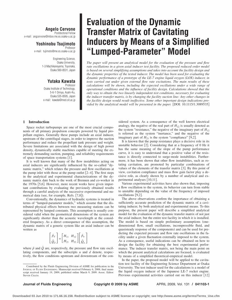
Angelo CervonePostdoctoral Fellow


Yoshinobu TsujimotoProfessor


Engineering Science,Osaka University,

1-3 Machikaneyama, Toyonaka,Osaka 560-8531, Japan

Yutaka KawataProfessor

Osaka Institute of Technology,5-6-1 Omiya, Asahi-Ku,Osaka 535-8505, Japan


Evaluation of the DynamicTransfer Matrix of CavitatingInducers by Means of a Simplified“Lumped-Parameter” ModelThe paper will present an analytical model for the evaluation of the pressure and flowrate oscillations in a given axial inducer test facility. The proposed reduced order modelis based on several simplifying assumptions and takes into account the facility design andthe dynamic properties of the tested inducer. The model has been used for evaluating thedynamic performance of a prototype of the LE-7 engine liquid oxygen (LOX) inducer, intests carried out under given external flow rate excitations. The main results of thesecalculations will be shown, including the expected oscillations under a wide range ofoperational conditions and the influence of facility design. Calculations showed that theonly way to obtain the two linearly independent test conditions, necessary for evaluatingthe inducer transfer matrix, is by changing the facility suction line: Any other changes inthe facility design would result ineffective. Some other important design indications pro-vided by the analytical model will be presented in the paper. �DOI: 10.1115/1.3089535�

1 IntroductionSpace rocket turbopumps are one of the most crucial compo-

nents of all primary propulsion concepts powered by liquid pro-pellant engines. Generally these pumps include an axial inducer,upstream of the centrifugal stages, in order to improve the suctionperformance and reduce the propellant tank pressure and weight.Severe limitations are associated with the design of high powerdensity, dynamically stable machines capable of meeting the ex-tremely demanding suction, pumping, and reliability requirementsof space transportation systems �1�.

It is well known that many of the flow instabilities acting onaxial inducers are significantly influenced by the so-called “dy-namic matrix,” which relates the pressure and flow oscillations atthe pump inlet with those at the pump outlet �2–4�. The first stepsin the analytical and experimental characterizations of the dy-namic matrix date back to the work of Brennen and co-worker inthe 1970s �5,6�. However, more recent works have given impor-tant contributions by evaluating the previously obtained resultsthrough a careful analysis of the successive experimental and nu-merical data �see, for example, Refs. �7,8��.

Conventionally, the dynamics of hydraulic systems is treated interms of “lumped-parameter models,” which assume that the dis-tributed physical effects between two measuring stations can berepresented by lumped constants. This assumption is usually con-sidered valid when the geometrical dimensions of the system aresignificantly shorter than the acoustic wavelength at the consid-ered frequency. As a direct consequence of this assumption, thedynamic matrix of a generic system like an axial inducer can bewritten as

� pd

Qd� = �H11 H12

H21 H22�� pu

Qu�

where p and Q are, respectively, the pressure and flow rate oscil-lating components, and the subscripts u and d denote, respec-tively, the flow conditions upstream and downstream of the con-

sidered system. As a consequence of the well known electricalanalogy, the negative of the real part of H12 is usually denoted asthe system “resistance,” the negative of the imaginary part of H12is referred as the system “inertance,” and the negative of theimaginary part of H21 is the system “compliance” �9,2�.

It is known that the pump resistance plays a decisive role in itsunstable behavior �2�. Considering that at a frequency of 0 Hz ithas the same meaning of the slope of the pump performancecurve, it is easy to understand that a positive value of the resis-tance is directly connected to surge-mode instabilities. Further-more, it has been shown that other flow instabilities, such as ro-tating cavitation, are promoted by particular combinations ofvalues of the elements of the transfer matrix �3�. By this point ofview, cavitation compliance and mass flow gain factor play a de-cisive role, as clearly shown by a number of analytical and ex-perimental analyses �10,11�.

Various experimental activities have also shown that, imposinga flow oscillation to the system, its behavior can turn from stableto unstable depending on the value of the frequency of imposedoscillations �9,2�.

The above observations confirm the importance of obtaining asufficiently accurate prediction of the dynamic matrix of a cavi-tating inducer, by both analytical and experimental means. To thispurpose, the present paper will describe a simplified analyticalmodel for the evaluation of the dynamic transfer matrix of not justthe axial inducer, but the entire test facility in which it is installed.The model is based on simple preliminary assumptions �one-dimensional flow, small oscillations, incompressible fluid, andquasisteady response of the components� and can be used for pre-dicting the expected pressure and flow rate oscillations in the fa-cility under a given fluctuation externally imposed to the system.As a consequence, useful indications can be obtained on how todesign the facility for obtaining the best experimental perfor-mance. The inducer transfer matrix, not being the main point onwhich the present analytical calculations are focused, is evaluatedby means of a simplified theoretical-empirical model.

In the paper, the proposed model will be applied to the cavita-tion test facility of the Engineering Science Department at OsakaUniversity. The test inducer used for the calculations is a model ofthe liquid oxygen inducer of the Japanese LE-7 rocket engine.Previous experimental activities carried out on this inducer �12�

Contributed by the Fluids Engineering Division of ASME for publication in theJOURNAL OF FLUIDS ENGINEERING. Manuscript received February 6, 2008; final manu-script received January 19, 2009; published online March 9, 2009. Assoc. Editor:Steven Ceccio.



have shown that several flow instabilities are promoted by thecavitating pattern on the pump. The experiments, mainly focusedon the characterization of the different flow instabilities acting onthe inducer and their field of existence, lead to the detection ofinstabilities including rotating cavitation, asymmetric blade cavi-tation, and higher order modes. It has also been shown that someof these instabilities can be reduced or suppressed by changing thecasing geometry: Rotating cavitation and asymmetric cavitation,as an example, are strongly reduced by means of a J-groove onthe casing.

2 Experimental ApparatusA sketch of the cavitation facility of the Engineering Science

Department at Osaka University is shown in Fig. 1. The figurealso shows the main notations, which will be used in the presentpaper.

The actual sections where the pressure and flow rate oscilla-tions are measured are denoted by subscripts 1 �upstream of theinducer� and 2 �downstream of the inducer�. The sector of thefacility included between these two points will be referred in thefollowing as “measurement section.” A given external flow rateoscillation �denoted by QF� is imposed just downstream of themeasurement point 2, by means of a dedicated apparatus. Thesuction line �between tank and upstream measurement point� isdenoted by subscript C, while the discharge line �between thefluctuator and the main tank entrance� is denoted by subscript B.The internal pipe diameter is 203.5 mm in the suction and dis-charge lines and 155.2 mm inside the measurement section. Aconical expansion is installed downstream the fluctuator, while aconical contraction is present just after the measurement point 1.Two valves for the regulation of the flow rate are mounted in thedischarge section.

The test inducer used for the present calculations �Fig. 2� is amodel of the liquid oxygen inducer of the Japanese LE-7 rocketengine. It is a three-bladed axial inducer, with a tip radius rT=74.9 mm and a profiled, variable-radius hub �the hub/tip radiiratio is 0.25 at the inlet and 0.51 at the outlet�. The inlet tip bladeangle is 7.5 deg and the tip solidity is 1.91.

3 Model DescriptionThe proposed model is based on the following initial assump-

tions.

�1� The flow is assumed unsteady, quasi-one-dimensional.�2� All oscillations are assumed to be small �only first order

terms are taken into account in the equations�.�3� The working fluid is assumed incompressible and compli-

ance is therefore considered negligible, except for regionswhere cavitation or air volumes are present.

�4� The response of all components of the system is assumedquasisteady. Even if it has been widely shown that this

assumption is not valid in real pumps under cavitating con-ditions �7,8,11�, it could represent a good starting point forthe simplified reduced order analysis presented in this pa-per. As it will be shown in the following, the results and themain conclusions drawn by the analyses are not signifi-cantly affected by this assumption, especially for what con-cerns the design of the experiment.

Under the above assumptions, pressure and flow rate can bewritten in a complex form, as functions of time, as follows:

p�t� = p + p · ei�t

Q�t� = Q + Q · ei�t

where p and Q �usually real� are the pressure and flow rate

steady values, p and Q �usually complex� are the pressure andflow rate oscillating components, and � is the frequency of theoscillations.

The relevant components for the evaluation of the dynamic ma-trix are the oscillating ones. Under the above assumptions, thematrices of all the components of the facility can be easily evalu-ated as follows.

Fig. 1 Schematic of the experimental facility

Fig. 2 The test inducer



3.1 Pipes. With a suitable manipulation of the generic conti-nuity and momentum equations, the dynamic matrix can be writ-ten as follows:

H = �1 − R − i�L

0 1�

where the resistance R and the inertance L are given by

R = k�Qu

Au2 + �� 1

Ad2 −

1

Au2�Qu

L = �1

�

in which � is the density of the working fluid, A is the pipesection, � is the “inertial length” of the pipe �defined as the meanpipe section divided to pipe length�, and k is the loss coefficientinside the pipe.

3.2 Main Tank. In this case, the dynamic matrix is given by

H = � 1 0

− i�C 1�

where the compliance C is

C =V

�p

in which p and V are the mean pressure and volume of the air atthe top of the tank, and � is the specific heat ratio of air.

3.3 Inducer. In the noncavitating case, it can be shown thatthe inducer dynamic matrix is very simple, with a similar structureto that of pipe sections. In this case the inertance L is simply givenby the inertial length of blade passages, while the resistance R canbe evaluated using the momentum equation as follows:

R = −��rT

Au

d�

d�+ �Qu� 1

Ad2 −

1

Au2�

in which � is the inducer rotating speed, rT is the inducer tipradius, and d� /d� is the slope of the inducer performance curve.

In the cavitating case the equations become more complicated.The driving parameter is the presence of a vapor region on theblades, the oscillations of which generate a shift between the inletand outlet flow oscillations. The evaluation of the volume of cav-ity formed inside the pump, as a function of the flow coefficient �and the cavitation number �, is therefore needed. Elaboration ofthe continuity and momentum equations shows that the dynamicmatrix is

H = �1 − �S + i�X� − R − i�L

− i�C 1 − i�M�

where S+ i�X is the pressure gain factor, R+ i�L is the pumpimpedance, C is the cavitation compliance, and M is the massflow gain factor. These parameters are defined as follows:

S + i�X = − 2 ��

��

�

+ CLind�2 − i��Qu

Ad2 C −

��rT

Ad ��

��

�

C�R + i�L = −

��rT

Ad ��

��

�

− �Qu� 1

Au2 −

1

Ad2� + MLind�

2

− i�M��Qu

Ad2 −

��rT

Ad ��

��

�

� + i�Lind

C = −2

��2rT2 �VC

��

�

M = −1

Au�rT �VC

��

�

in which VC is the cavity volume and Lind is the inertance ofinducer blade passages.

After having tried different approaches for the evaluation of thecavity volume VC, including suitable modifications to theBrennen–Acosta model of partially cavitating cascades �13,14�, asimpler empirical-theoretical model will be proposed here. Thechoice of this model was led by the consideration that the presentwork is not aimed to an accurate evaluation of the inducer dy-namic characteristics, but to a characterization of the entire facil-ity, in order to acquire useful theoretical and design indications forthe successive experimental activities.

The cavitation volume has therefore been estimated using apolynomial relationship and taking into account the experimentaldata provided by Brennen for a 10.2 cm inducer �13�. Consideringthat these data give an estimation of the cavitation compliance onthe inducer at four different values of �, the following relationwas used:

VC��,�� = a1�� − �c�4 + a2�� − �c�3 + a3�� − �c�2 + a4�� − �c�

+ VC��c�

where the constants a1, a2, a3, and a4 can be evaluated usingthe four experimental values of C�� provided by Brennen �13�.In the above equation, �c is the “choked cavitation number” of theBrennen–Acosta partially cavitating cascade model �i.e., the cavi-tation number for which the cavity becomes infinitely long �13��,which depends on the inducer geometry and the incidence angleand, as a consequence, the flow coefficient.

The cavity volume at the choked cavitation number, VC��c�, isevaluated assuming the following.

�1� At the choked cavitation number �c, complete breakdownoccurs �i.e., the head rise of the inducer falls to zero�.

�2� At �c, the blade channels are completely filled by bubblycavitation, having a void fraction 0, which can be evalu-ated using the relationship shown by Brennen �5�,

� =0�2 − 0��2

2�1 − 0�2 sin2 �b

where �b is the tip blade angle and � is the amount ofbreakdown, estimated using assumption �1�.

�3� The cavity volume at choked cavitation number is finallyestimated by multiplying the void fraction 0 to the bladechannel volume.

Calculations confirmed that the model can reasonably repro-duce the experimental transfer matrix as shown in Ref. �13�.

3.4 Characterization of the Complete Facility. Four un-knowns have to be evaluated for the solution of the problem: thepressure and flow oscillations at the inlet measurement point, p1

and Q1, and the correspondent oscillations at the outlet measure-

ment point, p2 and Q2. The first two equations for their evaluationcan be obtained by considering the equilibrium inside the mea-surement section

� p2

Q2� = �HM11 HM12

HM21 HM22�� p1

Q1�

where the transfer matrix HM is given by

HM = �1 − Rout − i�Lout

0 1��1 − �S + i�X� − Rind − i�Lind

− i�Cind 1 − i�M�

��1 − Rin − i�Lin

0 1�



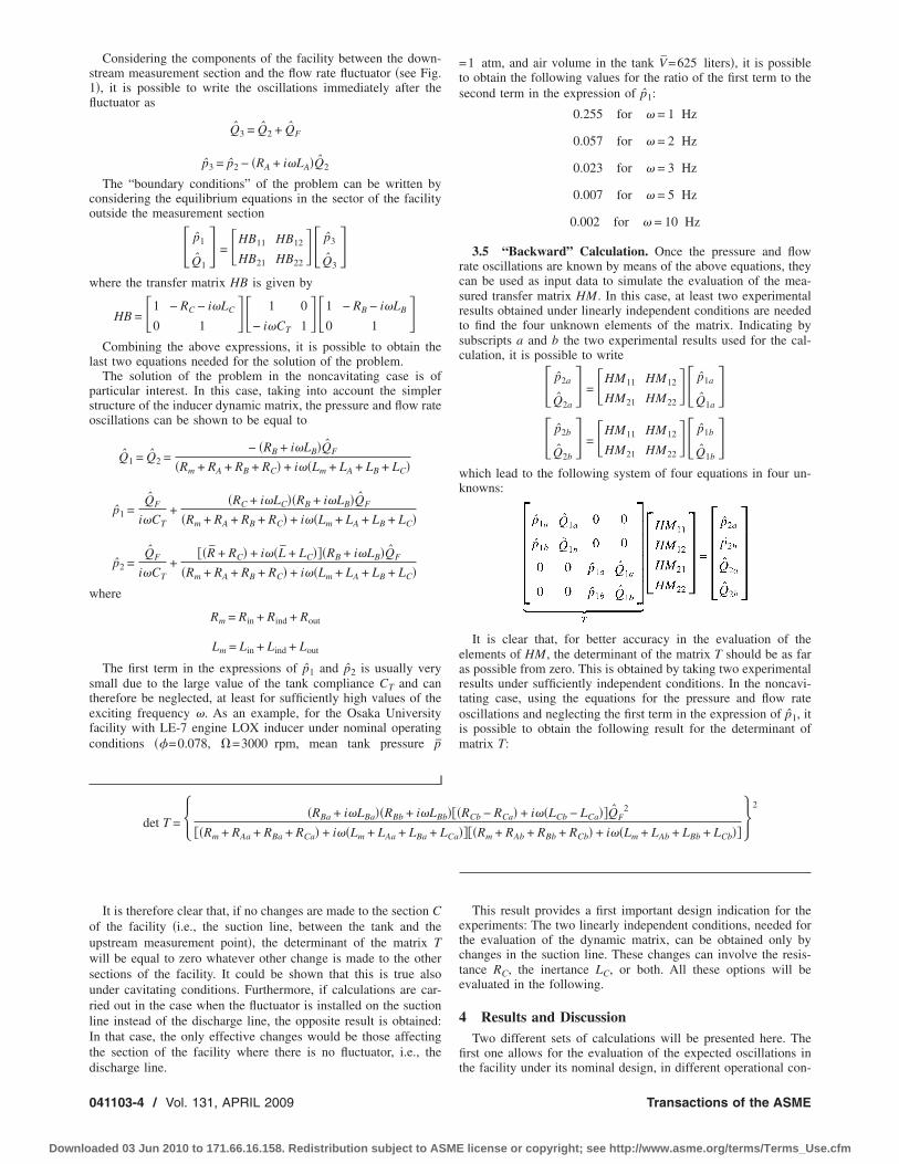
Considering the components of the facility between the down-stream measurement section and the flow rate fluctuator �see Fig.1�, it is possible to write the oscillations immediately after thefluctuator as

Q3 = Q2 + QF

p3 = p2 − �RA + i�LA�Q2

The “boundary conditions” of the problem can be written byconsidering the equilibrium equations in the sector of the facilityoutside the measurement section

� p1

Q1� = �HB11 HB12

HB21 HB22�� p3

Q3�

where the transfer matrix HB is given by

HB = �1 − RC − i�LC

0 1�� 1 0

− i�CT 1��1 − RB − i�LB

0 1�

Combining the above expressions, it is possible to obtain thelast two equations needed for the solution of the problem.

The solution of the problem in the noncavitating case is ofparticular interest. In this case, taking into account the simplerstructure of the inducer dynamic matrix, the pressure and flow rateoscillations can be shown to be equal to

Q1 = Q2 =− �RB + i�LB�QF

�Rm + RA + RB + RC� + i��Lm + LA + LB + LC�

p1 =QF

i�CT+

�RC + i�LC��RB + i�LB�QF


p2 =QF

i�CT+

��R + RC� + i��L + LC��RB + i�LB�QF


where

Rm = Rin + Rind + Rout

Lm = Lin + Lind + Lout

The first term in the expressions of p1 and p2 is usually verysmall due to the large value of the tank compliance CT and cantherefore be neglected, at least for sufficiently high values of theexciting frequency �. As an example, for the Osaka Universityfacility with LE-7 engine LOX inducer under nominal operatingconditions ��=0.078, �=3000 rpm, mean tank pressure p

=1 atm, and air volume in the tank V=625 liters�, it is possibleto obtain the following values for the ratio of the first term to thesecond term in the expression of p1:

0.255 for � = 1 Hz

0.057 for � = 2 Hz

0.023 for � = 3 Hz

0.007 for � = 5 Hz

0.002 for � = 10 Hz

3.5 “Backward” Calculation. Once the pressure and flowrate oscillations are known by means of the above equations, theycan be used as input data to simulate the evaluation of the mea-sured transfer matrix HM. In this case, at least two experimentalresults obtained under linearly independent conditions are neededto find the four unknown elements of the matrix. Indicating bysubscripts a and b the two experimental results used for the cal-culation, it is possible to write

� p2a

Q2a� = �HM11 HM12

HM21 HM22�� p1a

Q1a�

� p2b

Q2b� = �HM11 HM12

HM21 HM22�� p1b

Q1b�

which lead to the following system of four equations in four un-knowns:

It is clear that, for better accuracy in the evaluation of theelements of HM, the determinant of the matrix T should be as faras possible from zero. This is obtained by taking two experimentalresults under sufficiently independent conditions. In the noncavi-tating case, using the equations for the pressure and flow rateoscillations and neglecting the first term in the expression of p1, itis possible to obtain the following result for the determinant ofmatrix T:

det T = �RBa + i�LBa��RBb + i�LBb��RCb − RCa� + i��LCb − LCa��QF2

��Rm + RAa + RBa + RCa� + i��Lm + LAa + LBa + LCa��Rm + RAb + RBb + RCb� + i��Lm + LAb + LBb + LCb��2

It is therefore clear that, if no changes are made to the section Cof the facility �i.e., the suction line, between the tank and theupstream measurement point�, the determinant of the matrix Twill be equal to zero whatever other change is made to the othersections of the facility. It could be shown that this is true alsounder cavitating conditions. Furthermore, if calculations are car-ried out in the case when the fluctuator is installed on the suctionline instead of the discharge line, the opposite result is obtained:In that case, the only effective changes would be those affectingthe section of the facility where there is no fluctuator, i.e., thedischarge line.

This result provides a first important design indication for theexperiments: The two linearly independent conditions, needed forthe evaluation of the dynamic matrix, can be obtained only bychanges in the suction line. These changes can involve the resis-tance RC, the inertance LC, or both. All these options will beevaluated in the following.

4 Results and DiscussionTwo different sets of calculations will be presented here. The

first one allows for the evaluation of the expected oscillations inthe facility under its nominal design, in different operational con-



ditions. The second one will be a “backward” calculation, aimedto the estimation of the effectiveness of several alternative designsof the facility for obtaining the second linearly independent ex-perimental condition.

4.1 Nominal Design: Pressure and Flow Rate Oscillations.The 3D plots from Figs. 3–6 show the amplitude of pressure andflow rate fluctuations under cavitating conditions, as functions ofthe excitation frequency and the flow coefficient, for �=0.1, �=3000 rpm, and amplitude of the flow rate oscillations generatedby the fluctuator equal to 1 l/s. Since there is no phase informationin the 3D plots, Figs. 7–10 show the amplitude and phase ofpressure and flow rate fluctuations under cavitating conditions, asfunctions of the excitation frequency, for �=0.1, �=3000 rpm,�=0.078 �inducer nominal operating conditions�, and amplitudeof the flow rate oscillations generated by the fluctuator equal to 1l/s. The phase delay is calculated with respect to the flow rateoscillations generated by the fluctuator.

4.2 Evaluation of Alternative Facility Designs. The effec-tiveness of different facility designs has been evaluated by meansof the backward calculation. The results provided by the modelhave therefore been used as a starting point for the evaluation ofthe dynamic matrix elements, in order to compare this evaluationto the actual nominal values provided by the model. The dynamicmatrix elements have been evaluated at different excitation fre-quencies � and flow coefficients �.

In order to better simulate the real experimental conditions ex-pected in the facility, three different “artificial” error sources havebeen intentionally added to the nominal data. The first two errorsources are a random “white noise” at all the frequencies includedin the spectrum of the measured signal �which simulates the typi-cal white noise usually present in laboratory environments� and adefined sinusoidal noise at 60 Hz �frequency of electrical distur-bance in Japan�. The third error source consists in taking only afinite number of decimals from the numerical solutions providedby the model, in order to simulate the experimental sensors’ ac-curacy.

Fig. 3 Amplitude of the upstream pressure oscillations, as afunction of the excitation frequency � and the flow coefficient� „cavitating conditions…, for �=3000 rpm, �=0.1, and ampli-tude of the flow rate oscillations generated by the fluctuatorequal to 1 l/s

Fig. 4 Amplitude of the downstream pressure oscillations, asa function of the excitation frequency � and the flow coefficient� „cavitating conditions…, for �=3000 rpm, �=0.1, and ampli-tude of the flow rate oscillations generated by the fluctuatorequal to 1 l/s

Fig. 5 Amplitude of the upstream flow rate oscillations, as afunction of the excitation frequency � and the flow coefficient� „cavitating conditions…, for �=3000 rpm, �=0.1, and ampli-tude of the flow rate oscillations generated by the fluctuatorequal to 1 l/s

Fig. 6 Amplitude of the downstream flow rate oscillations, asa function of the excitation frequency � and the flow coefficient� „cavitating conditions…, for �=3000 rpm, �=0.1, and ampli-tude of the flow rate oscillations generated by the fluctuatorequal to 1 l/s



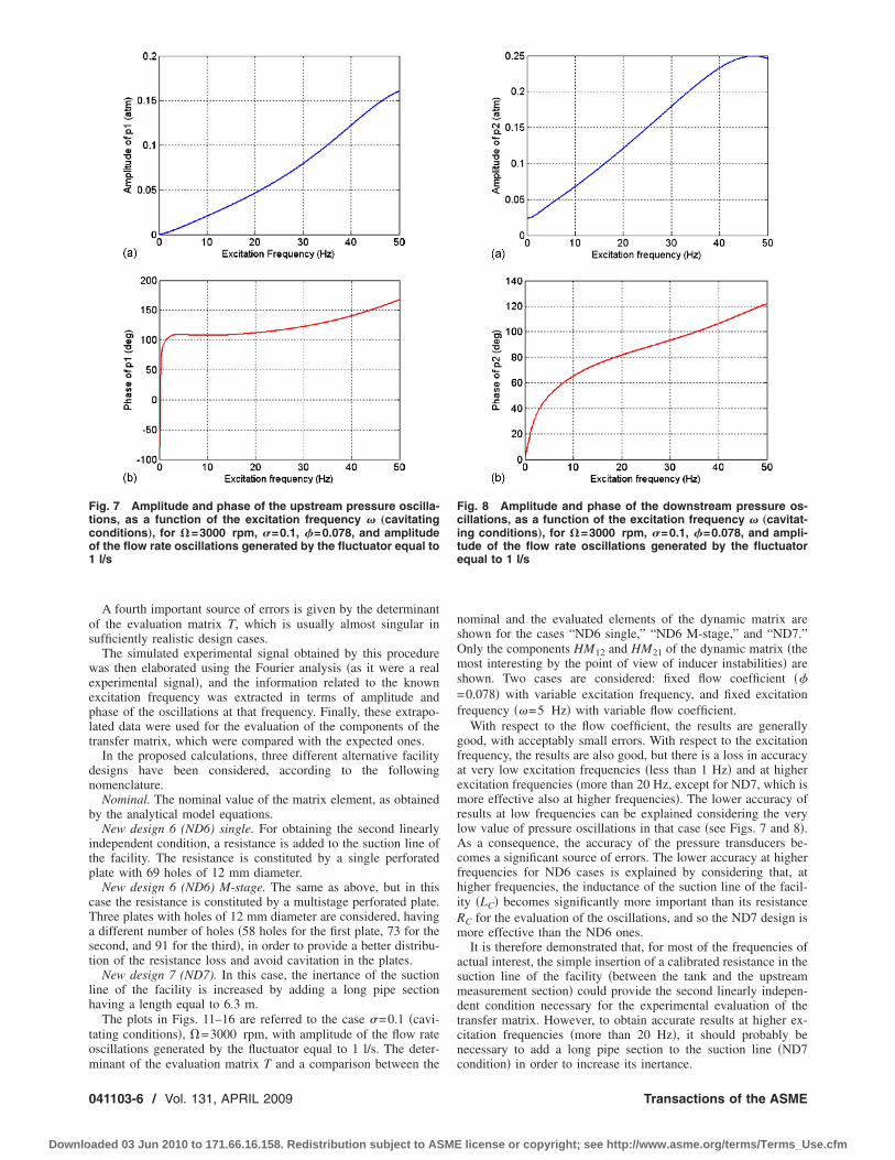
A fourth important source of errors is given by the determinantof the evaluation matrix T, which is usually almost singular insufficiently realistic design cases.

The simulated experimental signal obtained by this procedurewas then elaborated using the Fourier analysis �as it were a realexperimental signal�, and the information related to the knownexcitation frequency was extracted in terms of amplitude andphase of the oscillations at that frequency. Finally, these extrapo-lated data were used for the evaluation of the components of thetransfer matrix, which were compared with the expected ones.

In the proposed calculations, three different alternative facilitydesigns have been considered, according to the followingnomenclature.

Nominal. The nominal value of the matrix element, as obtainedby the analytical model equations.

New design 6 (ND6) single. For obtaining the second linearlyindependent condition, a resistance is added to the suction line ofthe facility. The resistance is constituted by a single perforatedplate with 69 holes of 12 mm diameter.

New design 6 (ND6) M-stage. The same as above, but in thiscase the resistance is constituted by a multistage perforated plate.Three plates with holes of 12 mm diameter are considered, havinga different number of holes �58 holes for the first plate, 73 for thesecond, and 91 for the third�, in order to provide a better distribu-tion of the resistance loss and avoid cavitation in the plates.

New design 7 (ND7). In this case, the inertance of the suctionline of the facility is increased by adding a long pipe sectionhaving a length equal to 6.3 m.

The plots in Figs. 11–16 are referred to the case �=0.1 �cavi-tating conditions�, �=3000 rpm, with amplitude of the flow rateoscillations generated by the fluctuator equal to 1 l/s. The deter-minant of the evaluation matrix T and a comparison between the

nominal and the evaluated elements of the dynamic matrix areshown for the cases “ND6 single,” “ND6 M-stage,” and “ND7.”Only the components HM12 and HM21 of the dynamic matrix �themost interesting by the point of view of inducer instabilities� areshown. Two cases are considered: fixed flow coefficient ��=0.078� with variable excitation frequency, and fixed excitationfrequency ��=5 Hz� with variable flow coefficient.

With respect to the flow coefficient, the results are generallygood, with acceptably small errors. With respect to the excitationfrequency, the results are also good, but there is a loss in accuracyat very low excitation frequencies �less than 1 Hz� and at higherexcitation frequencies �more than 20 Hz, except for ND7, which ismore effective also at higher frequencies�. The lower accuracy ofresults at low frequencies can be explained considering the verylow value of pressure oscillations in that case �see Figs. 7 and 8�.As a consequence, the accuracy of the pressure transducers be-comes a significant source of errors. The lower accuracy at higherfrequencies for ND6 cases is explained by considering that, athigher frequencies, the inductance of the suction line of the facil-ity �LC� becomes significantly more important than its resistanceRC for the evaluation of the oscillations, and so the ND7 design ismore effective than the ND6 ones.

It is therefore demonstrated that, for most of the frequencies ofactual interest, the simple insertion of a calibrated resistance in thesuction line of the facility �between the tank and the upstreammeasurement section� could provide the second linearly indepen-dent condition necessary for the experimental evaluation of thetransfer matrix. However, to obtain accurate results at higher ex-citation frequencies �more than 20 Hz�, it should probably benecessary to add a long pipe section to the suction line �ND7condition� in order to increase its inertance.

Fig. 7 Amplitude and phase of the upstream pressure oscilla-tions, as a function of the excitation frequency � „cavitatingconditions…, for �=3000 rpm, �=0.1, �=0.078, and amplitudeof the flow rate oscillations generated by the fluctuator equal to1 l/s

Fig. 8 Amplitude and phase of the downstream pressure os-cillations, as a function of the excitation frequency � „cavitat-ing conditions…, for �=3000 rpm, �=0.1, �=0.078, and ampli-tude of the flow rate oscillations generated by the fluctuatorequal to 1 l/s



Fig. 9 Amplitude and phase of the upstream flow rate oscilla-tions, as a function of the excitation frequency � „cavitatingconditions…, for �=3000 rpm, �=0.1, �=0.078, and amplitudeof the flow rate oscillations generated by the fluctuator equal to1 l/s

Fig. 10 Amplitude and phase of the downstream flow rate os-cillations, as a function of the excitation frequency � „cavitat-ing conditions…, for �=3000 rpm, �=0.1, �=0.078, and ampli-tude of the flow rate oscillations generated by the fluctuatorequal to 1 l/s

Fig. 11 Determinant of the evaluation matrix T, as a functionof the excitation frequency �, for �=3000 rpm, �=0.1, �=0.078, and amplitude of the flow rate oscillations generated bythe fluctuator equal to 1 l/s

Fig. 12 Real and imaginary parts of the element HM12 of thedynamic matrix, as functions of the excitation frequency �, for�=3000 rpm, �=0.1, �=0.078, and amplitude of the flow rateoscillations generated by the fluctuator equal to 1 l/s

Fig. 13 Real and imaginary parts of the element HM21 of thedynamic matrix, as functions of the excitation frequency �, for�=3000 rpm, �=0.1, �=0.078, and amplitude of the flow rateoscillations generated by the fluctuator equal to 1 l/s



5 ConclusionsAn analytical model for the evaluation of the dynamic matrix of

a cavitating inducer facility has been proposed in the present pa-per. The model, even if extremely simplified and based on verystrong assumptions, has shown to be a powerful tool for the de-sign of the facility and the preparation of the experimental activ-ity.

In particular, the backward calculation �utilization of the modelresults as simulated experimental data, after having opportunelyadded to them artificial error sources� can be used to get ex-tremely useful indications about the effectiveness of different fa-cility designs. Furthermore, the model equations showed that theonly effective design changes for obtaining the second linearlyindependent condition, needed for the experimental evaluation ofthe dynamic matrix, are those related to the suction line of thefacility �or, conversely, the discharge line if the external fluctua-tions are provided to the suction line�.

Future improvements to the model could include, as an ex-ample, a better evaluation of the inducer dynamic matrix, basedon more accurate models than the simple empirical-theoretical

model proposed in this paper. As a useful tool to this purpose, anextensive experimental activity is foreseen during the nextmonths, in order to measure the pressure and flow rate oscillationsin the facility under several operating conditions and compare theobtained data to the results of the model.

AcknowledgmentA.C. would like to acknowledge the support of Japan Society

for the Promotion of Science �JSPS�, which has funded his re-search program at Osaka University. He also expresses his grati-tude to all the colleagues at Pisa University in Italy, and, in par-ticular, Professor Luca d’Agostino and Professor MarianoAndrenucci, for their kind and constant encouragement.

Nomenclatureai constants in cavity volume equation,

i=1–4 �m3�A pipe section �m2�C compliance �m4 s2 /kg�k loss coefficient �dimensionless�L inertance �kg /m4�

M mass flow gain factor �s−1�p pressure �Pa�H generic dynamic matrix

HB dynamic matrix outside the measurementsection

HM dynamic matrix of the measurement sectionQ flow rate �m3 /s�

QF externally imposed flow oscillation �m3 /s�R resistance �kg /m4 s�rT inducer tip radius �m�S real part of the pressure gain factor

�dimensionless�t time �s�

T characteristic matrix for backward calculationV volume �m3�

VC cavity volume �m3�X imaginary part of the pressure gain factor �s�

0 void fraction �dimensionless��b inducer tip blade angle �rad�

� head loss at breakdown �dimensionless�� flow coefficient �dimensionless�� specific heat ratio �dimensionless�

Fig. 14 Determinant of the evaluation matrix T, as a functionof the flow coefficient �, for �=3000 rpm, �=0.1, �=5 Hz, andamplitude of the flow rate oscillations generated by the fluctua-tor equal to 1 l/s

Fig. 15 Real and imaginary parts of the element HM12 of thedynamic matrix, as functions of flow coefficient �, for �=3000 rpm, �=0.1, �=5 Hz, and amplitude of the flow rate os-cillations generated by the fluctuator equal to 1 l/s

Fig. 16 Real and imaginary parts of the element HM21 of thedynamic matrix, as functions of flow coefficient �, for �=3000 rpm, �=0.1, �=5 Hz, and amplitude of the flow rate os-cillations generated by the fluctuator equal to 1 l/s



� inertial length �m�� head coefficient �dimensionless�� density �kg /m3�� cavitation number �dimensionless�

�c “choked” cavitation number �dimensionless�� frequency of oscillations �Hz�� inducer rotating speed �rad/s�

Superscriptsˆ oscillating component of a given quantity

steady component of a given quantity

Subscriptsa ,b linearly independent experimental conditions

A pipework from measurement section tofluctuator

B discharge lineC suction lined downstream section �generic�

in measurement section �upstream of inducer�ind inducer

m total measurement section �including inducer�out measurement section �downstream of inducer�

T main tanku upstream section �generic�1 upstream measurement point2 downstream measurement point3 point immediately after the fluctuator

References�1� Stripling, L. B., and Acosta, A. J., 1962, “Cavitation in Turbopumps–Part 1,”

ASME J. Basic Eng., 84, pp. 326–338.�2� Kawata, Y., Takata, T., Yasuda, O., and Takeuchi, T., 1988, “Measurement of

the Transfer Matrix of a Prototype Multi-Stage Centrifugal Pump,” Paper No.C346/88.

�3� Tsujimoto, Y., Kamijo, K., and Yoshida, Y., 1993, “A Theoretical Analysis ofRotating Cavitation in Inducers,” ASME J. Fluids Eng., 115, pp. 135–141.

�4� Tsujimoto, Y., Watanabe, S., and Horiguchi, H., 1998, “Linear Analyses ofCavitation Instabilities of Hydrofoils and Cascades,” Proceedings of the US-Japan Seminar: Abnormal Flow Phenomena in Turbomachinery, Osaka, Japan.

�5� Brennen, C. E., 1978, “Bubbly Flow Model for the Dynamic Characteristics ofCavitating Pumps,” J. Fluid Mech., 89, pp. 223–240.

�6� Ng, S. L., and Brennen, C. E., 1978, “Experiments on the Dynamic Behaviorof Cavitating Pumps,” ASME J. Fluids Eng., 100, pp. 166–176.

�7� Otsuka, S., Tsujimoto, Y., Kamijo, K., and Furuya, O., 1996, “Frequency De-pendence of Mass Flow Gain Factor and Cavitation Compliance of CavitatingInducers,” ASME J. Fluids Eng., 118, pp. 400–408.

�8� Rubin, S., 2004, “An Interpretation of Transfer Function Data for a CavitatingPump,” Proceedings of the 40th AIAA/ASME/SAE/ASEE Joint PropulsionConference, Fort Lauderdale, FL.

�9� Bhattacharyya, A., 1994, “Internal Flows and Force Matrices in Axial FlowInducers,” Ph.D. thesis, California Institute of Technology, Pasadena, CA.

�10� Jun, S. I., Tokumasu, T., and Kamijo, K., 2003, “Dynamic Response Analysisof High Pressure Rocket Pumps,” Proceedings of CAV2003—Fifth Interna-tional Symposium on Cavitation, Osaka, Japan.

�11� Yamamoto, K., and Tsujimoto, Y., 2008, “Backflow Vortex Cavitation and ItsEffects on Cavitation Instabilities,” Proceedings of the WIMRC CavitationForum, Warwick University, Coventry, UK.

�12� Shimiya, N., Fujii, A., Horiguchi, H., Uchiumi, M., Kurokawa, J., andTsujimoto, Y., 2006, “Suppression of Cavitation Instabilities in an Inducer byJ-Groove,” Proceedings of CAV2006—Sixth International Symposium onCavitation, Wageningen, The Netherlands.

�13� Brennen, C. E., 1994, Hydrodynamics of Pumps, Concepts ETI Inc., Norwich,VT/Oxford University Press, Oxford.

�14� Brennen, C. E., and Acosta, A. J., 1973, “Theoretical, Quasi-Static Analysis ofCavitation Compliance in Turbopumps,” J. Spacecr. Rockets, 10�3�, pp. 175–179.



James R. DeBonis1

Inlet and Nozzle Branch,NASA Glenn Research Center,

Cleveland, OH 44135e-mail: [email protected]

RANS Analyses of TurbofanNozzles With Internal WedgeDeflectors for Noise ReductionComputational fluid dynamics (CFD) was used to evaluate the flow field and thrustperformance of a promising concept for reducing the noise at take-off of dual-streamturbofan nozzles. The concept, offset stream technology, reduces the jet noise observed onthe ground by diverting (offsetting) a portion of the fan flow below the core flow, thick-ening and lengthening this layer between the high-velocity core flow and the groundobservers. In this study a wedge placed in the internal fan stream is used as the diverter.Wind, a Reynolds averaged Navier–Stokes (RANS) code, was used to analyze the flowfield of the exhaust plume and to calculate nozzle performance. Results showed that thewedge diverts all of the fan flow to the lower side of the nozzle, and the turbulent kineticenergy on the observer side of the nozzle is reduced. This reduction in turbulent kineticenergy should correspond to a reduction in noise. However, because all of the fan flow isdiverted, the upper portion of the core flow is exposed to the freestream, and the turbulentkinetic energy on the upper side of the nozzle is increased, creating an unintended noisesource. The blockage due to the wedge reduces the fan mass flow proportional to itsblockage, and the overall thrust is consequently reduced. The CFD predictions are invery good agreement with experimental flow field data, demonstrating that RANS CFDcan accurately predict the velocity and turbulent kinetic energy fields. While this initialdesign of a large scale wedge nozzle did not meet noise reduction or thrust goals, thisstudy identified areas for improvement and demonstrated that RANS CFD can be used toimprove the concept. �DOI: 10.1115/1.3089536�

1 IntroductionThe concept of offsetting the fan stream of a dual flow turbofan

nozzle to reduce jet noise was developed by Papamoschou at theUniversity of California Irvine �UCI� �1–3�. The idea is to providea thicker layer of fan flow on the lower �observer� side of thenozzle. The additional fan flow serves to extend the length of thefan stream covering or “shielding” a larger portion of the coreflow on the lower side. This layer of low speed flow reduces theconvective Mach number of the turbulent eddies generated by thehigh speed core flow. This reduces these turbulent structures’ abil-ity to generate strong acoustic waves that travel to the far field �onthe lower side of the nozzle�. Papamoschou’s �1–3� initial conceptwas to physically offset the nozzle flow paths. This eccentricnozzle would be difficult to implement in a real system. He foundthat vanes and/or wedges placed in the fan stream can deflect thefan flow to the lower portion of the jet to achieve the desired flowfield and resulting acoustics in a simple, easy to implement man-ner.

Papamoschou �1–3� tested these concepts in a small jet facility�1 in. �2.54 cm� fan exit diameter� and measured jet noise reduc-tions of over 5.0 dB in the overall sound pressure level. Theseimpressive results led the National Aeronautics and Space Admin-istration �NASA� to examine this noise reduction concept at alarger scale. NASA developed the Offset Stream Technology�OST� program to design and test turbofan nozzles with devices tooffset the fan flow. The program consisted of computational fluiddynamics �CFD� analysis to screen flow deflector design andplacement and to estimate nozzle performance, design of experi-ments �DOE� methodology to reduce the number of experimental

test points required, additional small scale testing, and large scaletesting �9.63 in. �24.5 cm� fan exit diameter� in the NASA GlennNozzle Acoustic Test Rig �NATR� �4�.

There are four other papers from the OST study that form acomplete description of the program. A companion CFD studyexamining the vane deflector and s-duct nozzles was performedby Dippold et al. �5�. The experimental results from NATR, acous-tics and particle image velocimetry �PIV�–based velocity mea-surements in the exhaust plume, were reported by Brown et al.�6�, and a comparison of experimental results between UCI andNASA Glenn was detailed by Zaman et al. �7�. The results of theDOE study were reported by Henderson et al. �8�.

The experimental results at NATR indicate that the wedge de-flectors do reduce the noise on the lower side of the nozzle atdownstream angles. However, at other angles on the lower sideand at all angles on the sideline and upper side, the noise wasincreased. In general, the overall estimated perceived noise level�EPNL� increased relative to the baseline due to the higher noiseat the other locations. One configuration, BPR=5.0, M�=0.0,showed a small noise reduction of 0.8 EPN dB. Based on mea-surements of turbulent kinetic energy, Brown et al. �6� concludedthat the wedge designs tested were too aggressive.

Thrust performance is a critical factor in assessing low noisenozzle concepts. Papamoschou �1–3� estimated the thrust loss innozzles with vane deflectors based on airfoil drag and nozzle flowdeflection �2�, and Papamoschou et al. �9� experimentally exam-ined the aerodynamics of a wedge deflector in a simplified con-figuration. But up to this point, there has been no detailed exami-nation of the performance of these nozzles. The NATR tests didnot include force measurements. A key element of the CFD cal-culations presented here was to characterize the thrust of thesenozzles and compare them to a baseline nozzle without deflectors.This work represents the highest fidelity estimates of OffsetStream nozzle performance to date.

This paper describes the CFD analyses performed to supportthe design and testing of turbofan nozzles with the wedge shaped

1Corresponding author.Contributed by the Fluids Engineering Division of ASME for publication in the

JOURNAL OF FLUIDS ENGINEERING. Manuscript received March 21, 2008; final manu-script received January 22, 2009; published online March 9, 2009. Assoc. Editor: ZviRusak. Paper presented at the AIAA Aerospace Sciences Meeting, 2008.



flow deflectors. The CFD analyses consisted of three parts: �1�pretest predictions to verify the wedge design and its effect on theflow field, �2� performance calculations to examine the perfor-mance penalties due to the noise reduction scheme, and �3� vali-dation of the CFD methodology against experimental data. Whileestimates of jet noise cannot be obtained directly from the CFDanalyses, the predicted levels of turbulent kinetic energy can beused to infer the impact of the wedge deflector on the noise fieldat a rudimentary level.

2 Description of Nozzles and Flow ConditionsThe nozzles used in this study were originally designed for

NASA under the Advanced Subsonic Technology program for in-vestigating mixing enhancement devices to reduce jet noise �10�.The baseline nozzles with no mixing devices were used here. Forthis study a wedge flow deflector was placed in the fan stream.The wedge sits completely inside the nozzle, and the base of thewedge is coincident with the nozzle exit �Fig. 1�. Three differentnozzles were analyzed: 3BB, 4BB, and 5BB �Fig. 2�. The 3BBand 5BB nozzles both have an external nozzle plug in the corestream and have nozzle bypass ratios �BPR� of 5 and 8, respec-tively. These two nozzles share the same fan flow geometry. The

core flow nozzle section was replaced to affect the bypass ratiochange. The 4BB nozzle has an internal plug in the core flow andhas a bypass ratio of 8. This nozzle was studied computationallybut not tested in the experiment. All three nozzles have the samefan diameter of 9.63 in. �24.5 cm�.

The shape of the wedge deflector studied here is the same as thewedge used by Papamoschou �1–3� in his initial studies. Thewedge has a half angle of 11 deg and a base width of 3.44 in.�8.74 cm�. The upper and lower surfaces of the wedge conform tothe internal contours of the fan stream. The wedge reduces the exitarea of the fan stream by 14%.

It is anticipated that the wedge deflector would be incorporatedas a pair of flaps into the existing structure of the engine. Forunderwing mounted engines found on most large transport air-craft, the flaps could be placed in the pylon. For other installa-tions, side mounted or more highly integrated installations, theflaps could be incorporated into a strut. In either case the flapswould deploy to form a wedge on take-off and retract for cruise.The pylons for underwing mounted engines already deflect somefan flow. However, additional flow deflection is probably neces-sary to maximize noise reduction.

The calculations performed for the pretest predictions and per-formance analyses were done using cycle data for a representativetake-off condition. Details of the operating conditions are in Table1. The experiment was run subsequent to the CFD analyses, andthe data were taken at slightly different conditions. The analyseswere rerun at these conditions for code validation purposes �Table2�. For the 3BB validation case, the nozzle was tested with staticfreestream conditions. This analysis was run with a freestreamMach number of 0.05 for numerical stability. Two 5BB cases wererun, one with heated streams and one with cold streams. Bothcases had a freestream Mach number of 0.20. Because the wedgedeflectors will most likely be removed from the flow after take-off, only that flight condition was analyzed.

3 Analysis Procedure

3.1 Geometry Definition. The computational grids �Fig. 3�were generated using the Gridgen Version 15 software �11�. Thedatabase, which provides the geometry for the grid generator, wastaken directly from the computer aided drafting �CAD� file used todesign and build the experimental model hardware. The grids area structured multiblock type, with separate grid blocks represent-

Fig. 1 Turbofan nozzle with wedge installed in the fan stream

Fig. 2 Schematic drawings of NASA GRC turbofan nozzles



ing the following: �1� the internal primary flow path, �2� the ex-ternal primary flow path including the plug, �3� the internal sec-ondary flow path, �4� the external secondary flow path, �5� thenacelle, and �6� the jet plume region �Fig. 4�. Dimensions of thegrids are given in Table 3. At block interfaces the grids are notcontiguous, and a Roe-based zone coupling algorithm is used topass the fluxes between blocks.

The grids for the baseline nozzles with no wedge deflector wereplanar, taking advantage of the axisymmetric geometry. A total of66,734 points were used. The grids for the nozzles with the wedgedeflector were three dimensional: a 180 degree segment, takingadvantage of the symmetry about the xy-plane �vertical stream-wise� plane. A total of 6,072,794 grid points were used.

3.2 Flow Solution. The flow solver used for all the computa-tions was Wind version 5.0 �12�. Wind is a general purpose Rey-nolds averaged Navier–Stokes �RANS� equation solver. All thecalculations presented here used the same code options. The de-fault numerical scheme was used: implicit time stepping and asecond-order physical Roe scheme for stretched grids. Turbulence

was modeled using the Menter �13� shear stress transport �SST�model. No additional corrections �i.e., compressibility corrections�were used in the model.

Grid sequencing in all three computational directions was usedduring the flow solution. Sequencing solves the equations on areduced grid to speed convergence. The sequenced results are theninterpolated onto the finer grid for continued processing. Onelevel of sequencing involves removing every other grid point fromthe previous level. The solution started at two levels of sequencingand progressed to the full grid solution. Nozzle force measure-ments were monitored, and the sequencing was reduced when thenozzle force converged on that grid level. Nozzle force measure-ments between the final grid level and the next sequenced level

Table 2 Nozzle operating conditions for comparison to experiment

Nozzle BPR

Fan Core Freestream

NPRT0�K�

U�m/s� NPR

T0�K�

U�m/s�

p�

�kPa�T�

�K� M�

3BB hot 5.0 1.83 356 336 1.68 833 480 98.6 298 0.00a

5BB hot 8.0 1.62 356 303 1.42 832 399 98.6 298 0.205BB cold 8.0 1.42 298 239 1.86 298 311 98.6 298 0.20

aCFD analysis used M�=0.05 for numerical stability.

Table 1 Nozzle operating conditions for performance calculations

Nozzle BPR

Fan Core Freestream

NPRT0�K�

U�m/s� NPR

T0�K�

U�m/s�

p�

�kPa�T�

�K� M�

3BB 5.0 1.83 364 340 1.68 833 480 98.6 294 0.294BB 8.0 1.57 347 290 1.52 844 437 98.6 294 0.295BB 8.0 1.62 356 303 1.42 832 399 98.6 294 0.29

Fig. 3 Grid of the 5BB nozzle with wedge installed in the fanstream

Fig. 4 Grid blocking structure

Table 3 Dimensions of the computational grid

Block Axial Radial Azimuthal Total

1 73 45 91 298,9352 53 165 91 795,7953 65 45 91 266,1754 45 109 91 446,3555 69 45 91 282,5556 253 173 91 3,982,979

Wedge �3D� 6,072,794

Baseline 66,734



agreed within 1%, indicating that grid convergence was obtained.Local time stepping was used to achieve a steady state solution.For the 3BB case at near static ambient conditions �M�=0.05�,the solution did not converge in this manner. For this case thesolution was switched to global time stepping, and convergence toa steady state was achieved.

4 Results

4.1 Examination of the Flow Fields. The noise benefit of theoffset fan stream concept is predicated on reducing the convectiveMach number of the core stream instabilities by lengthening thefan stream to cover or shield a larger portion of the high speed

Fig. 5 Streamwise „xy-plane… contours of u-velocity, u /Uc, for 3BB nozzles




primary flow �14�. The increased interface between the primaryand secondary streams reduces the region of large velocity gradi-ents �between the core and surrounding flow� and thus reduces theconvective Mach number and the strength of the noise sources. Inthe context of the CFD solutions presented, the reduced velocitygradient lowers the resultant turbulent kinetic energy, which canbe related to the noise sources in jets �15�. This effect can be seenin the streamwise �xy-plane� velocity and turbulent kinetic energy

contours in Figs. 5–10. Data are presented for all three nozzles�3BB, 4BB, and 5BB�, and the results show that all three flowfields behave similarly.

Velocity contours in the streamwise planes compare the wedgenozzle to the baseline nozzle �Figs. 5–7�. These contours showthat the presence of the wedge directs the core flow upward andsignificantly shortens the core stream’s potential core. The layer offan flow on the underside of the jet plume is substantially thicker.


Fig. 8 Streamwise „xy-plane… contours of turbulent kinetic energy, k /Uc2, for 3BB nozzles



While it is difficult to quantify, the fan flow does appear to havelengthened. This can be seen by the presence of large regions offlow near the fan exit velocity �u /Uc=0.7� as far downstream asx /Df =6. A low-velocity region immediately behind the wedgeindicates that a large recirculation region is present there.

Turbulent kinetic energy contours in the streamwise planes areshown in Figs. 8–10. On the upper side of the exhaust plume,levels of k /Uc

2 are increased and the peak level has moved up-

stream, closer to the nozzle exit. On the lower side of the exhaustplume, the levels of k /Uc

2 have been reduced. This is the desiredeffect. A small local peak in turbulence levels is seen directlybehind the wedge, again indicating a separated region and poten-tial noise source.

The movement of the fan flow induced by the wedge deflectoris more easily seen in cross-planes downstream of the nozzle exit�Figs. 11–16�. The fan flow moves to the lower half of the exhaust





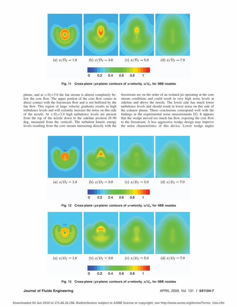
plume, and at x /Df =5.0 the fan stream is almost completely be-low the core flow. The upper portion of the core flow comes indirect contact with the freestream flow and is not buffered by thefan flow. This region of large velocity gradients results in highturbulence levels and will certainly increase the noise on this sideof the nozzle. At x /Df =3.0 high turbulence levels are presentfrom the top of the nozzle down to the sideline position �0–90deg, measured from the vertical�. The turbulent kinetic energylevels resulting from the core stream interacting directly with the

freestream are on the order of an isolated jet operating at the corestream conditions and could result in very high noise levels atsideline and above the nozzle. The lower side has much lowerturbulence levels and should result in lower noise on this side ofthe exhaust plume. These conclusions correspond well with thefindings in the experimental noise measurements �6�. It appearsthat the wedge moved too much fan flow, exposing the core flowto the freestream. A less aggressive wedge design may improvethe noise characteristics of this device. Lower wedge angles

Fig. 11 Cross-plane „yz-plane… contours of u-velocity, u /Uc, for 3BB nozzles





should be investigated to reduce the deflection of the fan flow.Also, shorter wedges that do not span the entire fan duct heightmay prevent the core flow from being completely exposed to thefreestream.

4.2 Nozzle Performance

4.2.1 Calculation Procedure. Nozzle performance was com-puted using the Wind utility, CFPOST. Stream thrust was com-

puted at the fan and core exits. Pressure and viscous forces werecomputed on the remaining surfaces: core nozzle lip, fan nozzlelip, plug, splitter between fan and core, nacelle, and wedge base.

Nozzle performance will be reported in two ways. First, thetotal thrust of the nozzle with wedge deflector will be expressed asa fraction of the baseline nozzle thrust

F/Fbaseline �1�

Fig. 15 Cross-plane „yz-plane… contours of turbulent kinetic energy, k /Uc2, for 4BB nozzles





Second, it will be expressed in terms of a thrust coefficient. Typi-cally nozzle performance results are reported using the grossthrust coefficient,

Cfg =Factual

mactualUideal

�2�

Using the actual mass flow in the denominator, Cfg, removes thedeviation from the ideal mass flow from the performance measure.Discharge coefficient is a separate measure for the reduction inmass flow,

Cd =mactual

mideal

�3�

For subsonic nozzles the mass flow through the nozzle can varydue to downstream effects, and the thrust coefficient does not givea true measure of nozzle performance. In these circumstances, thechange in the measured thrust is caused by the change in thenozzle flow rate and not a change in the exit velocity. This isespecially true for two-stream nozzles where the behavior of onestream can affect the flow rate of the other. Nozzles with noisesuppressing features can also affect flow rates. Therefore, a thrustcoefficient that accounts for the change in mass flow rate is usedin this paper. It is simply a thrust coefficient based on the idealmass flow rather than the actual mass flow. It can be convenientlywritten as the product of the gross thrust coefficient and dischargecoefficient,

Factual

midealUideal

=mactual

mideal

Factual

mactualUideal

= CdCfg �4�

For the cases where the wedge is installed in the nozzle, the idealmass flow is computed using the reduced nozzle exit area.

A baseline case, no wedge, was calculated for each nozzle ge-ometry. Performance of the wedge nozzles is referenced to thebaseline and is reported as ��CdCfg�,

��CdCfg� = �CdCfg�wedge − �CdCfg�baseline �5�

4.2.2 Performance Results. The thrust of the wedge nozzlesexpressed as a ratio to the baseline nozzle thrust is shown in Fig.17�a�. The wedge has created thrust losses between 11% and 13%.The reason for these losses is clear. Figure 17�b� shows the loss inmass flow of wedge nozzles, expressed as a ratio to the baselinenozzles. Total mass flow reduction also varies between 11% and13%. This reduction is due entirely to the reduction in fan massflow, which is approximately 14% for all three cases. These lossesare a direct result of the blockage created by the wedge �14% ofthe fan exit area�. For this noise reduction concept to be viable,the engine would have to be oversized to accommodate the per-formance penalty at take-off. Reducing the size of the wedge, assuggested for acoustic reasons, would reduce the thrust penalty.An alternative concept, placing the wedge external to the fannozzle on the splitter, has been proposed and should eliminate thisloss of fan mass flow �16�.

Fig. 17 Ratio of wedge nozzle to baseline nozzle performance

Fig. 18 Nozzle performance expressed as a thrust coefficient



Nozzle performance expressed as a thrust coefficient, CdCfg,for both the baseline and wedge configurations for all threenozzles is shown in Fig. 18�a�. For the wedge nozzles, this per-formance measure uses the ideal conditions based on the actual

exit area and therefore does not include the loss due to blockage.The external plug nozzles have uniformly higher performancethan the internal plug nozzle. Figure 18�b� shows the decrement inperformance due to the wedge. The losses due to the wedge vary

Fig. 19 Force breakout for 5BB baseline and wedge nozzles

Fig. 20 Streamlines for the 5BB nozzle



from about 0.7% to 1.1% and appear to be relatively low, consid-ering the large base area created by the wedge. A detailed break-out of the forces that comprise the thrust calculation is shown forthe 5BB baseline and wedge nozzles in Fig. 19. The figure con-firms that the primary loss mechanism is the loss in fan streamthrust due to the reduced mass flow. The presence of the wedgereduces the positive force on the nozzle plug and increases thedrag on the nacelle. The base drag on the wedge surface is arelatively minor component. This is somewhat surprising but canbe explained by the streamlines in Fig. 20. The figure shows thatthe flow that separates and recirculates behind the base of thewedge is the external flow over the nacelle. This also shows thelinkage between the presence of the wedge and the increased na-celle drag �Fig. 19�. The fan flow, the primary contributor to thethrust, is turned by the wedge to create the offset stream but doesnot separate behind the wedge, which would result in large thrustlosses.

By examining nozzle performance using the CdCfg parameter,we can see that the losses created by the wedge deflector would beacceptable if the reduction in mass flow could be removed oraccounted for in the nozzle design. The wedge deflector could be

Fig. 21 Component of the vertical thrust

Fig. 22 Comparison to experiment; u-velocity, u /Uc, for the 3BB nozzle with wedge, hot conditions



a viable noise reduction concept if the wedge size could be sig-nificantly reduced or if an external wedge that did not reduce thefan flow rate was employed.

The wedge induces a downward movement of the fan flow anda corresponding upward movement of the core flow. The resultingvertical component of the nozzle thrust is presented in Fig. 21.The data indicate that the wedge induces a very small verticalcomponent to the thrust. The external plug nozzles have a smallercomponent, about 0.5% of the axial thrust, and the internal plughas a slightly larger component, approximately 1.5% of the axialthrust.

The wedge deflector was one of three devices used to offset thefan stream examined in NASA’s OST program. The performanceof the other two devices, vane deflectors and s-duct nozzles, werealso analyzed using a similar CFD method �5�. The performanceof all three devices are compared in the Appendix of Ref. �17�.

4.3 Comparison to Experiment. Once the experimental testprogram was carried out, the CFD analyses were rerun to match

the experimental conditions. The same computational grids, codeversion, and code options were used. The experimental data werewithheld until the predictions were complete, and no attemptswere made to adjust code parameters to better match the data.

The nozzles were tested in the NASA Glenn NATR facility �4�.The NATR is a 53 in. �135 cm� diameter free jet facility with amaximum Mach number of 0.30. The nozzles were mounted inthe NATR on the high flow jet exit rig, which provides high pres-sure and high temperature air to both fan and core nozzle streams.The experimental data consisted of particle image velocimetrymeasurements of instantaneous velocity components in the nozzleplume �18�. The data were measured in planes parallel to thenozzle exit at distances of 1.0, 1.5, 2.0, 3.0, 5.0, and 7.0 fandiameters downstream of the fan nozzle exit. A complete descrip-tion of the experiment including both the PIV shown here and theacoustic measurements is given by Brown et al. �6�. The measuredu-velocity �axial component� and turbulent kinetic energy were

Fig. 23 Comparison to experiment; turbulent kinetic energy, k /Uc2, for the 3BB nozzle with wedge, hot

conditions



compared with the predictions for three wedge nozzle cases listedin Table 2. Comparisons for the baseline nozzle cases can befound in Ref. �17�.

The 3BB nozzle was tested at conditions similar to the pretestpredictions, but with a static freestream. The CFD analysis used asmall freestream velocity, M�=0.05, to prevent numerical insta-bilities. Plots showing the comparison between prediction and ex-periment for both axial velocity and turbulent kinetic energy areshown in Figs. 22 and 23. Near the fan exit plane at x /Df =1.0 and3.0, the proximity of the nozzle plug to the measurement planescaused a low signal to noise ratio in the experimental data. Thesedata were removed, resulting in the white regions in the center ofthe plots. The white areas at the corners of the experimental dataare due to the orientation of the nozzle relative to the PIV mea-surement plane. Overall, the agreement between CFD and experi-ment is very good. The contour plots indicate that the CFD does agood job of predicting the shape of the nozzle plume and themovement of diverted fan flow relative to the core. One does seethat the CFD predicts a more diffuse plume shape compared withexperiment. Line plots along the y-axis �vertical axis� show that

the CFD does a good job of predicting the levels of both velocityand turbulent kinetic energy. For this case the Wind code predictshigher peak velocities. This is due to the inclusion of the forwardvelocity in the freestream for numerical reasons. This small cof-low serves to reduce the nozzle mixing rate �19�.

The 5BB nozzle was tested at two different flow conditions.The quality of the PIV data near the nozzle exit was much betterwith only small regions at x /Df =1.0 where the data were re-moved. The first case had the same nozzle conditions as the pre-test prediction, but the freestream Mach number was 0.20 insteadof 0.29. The comparison is presented in Figs. 24 and 25. For thiscase agreement is very good for both velocity and turbulent ki-netic energy. The contour plots show similar agreement in plumeshape. The line plots show that there is excellent agreement in theprediction of both velocity and turbulence levels. The improvedagreement in the levels over the 3BB case is most likely due to thefact that the CFD analysis matched the experimental freestreamvelocity. The second 5BB case was tested at cold nozzle tempera-tures and a Mach 0.20 freestream. The comparison for this case ispresented in Figs. 26 and 27. Again, for all aspects agreement

Fig. 24 Comparison to experiment; u-velocity, u /Uc, for the 5BB nozzle with wedge, hot conditions



between experiment and predictions is very good.In general for all the cases, very good agreement is achieved

between the CFD and experiment in terms of plume shape, veloc-ity levels, and turbulent kinetic energy levels. The CFD predictsslightly higher values of velocity and slightly lower values ofturbulent kinetic energy at the downstream locations. This behav-ior is typical of RANS CFD predictions for jets using two-equation turbulence models �20�. The baseline nozzle cases re-ported in Ref. �17� similarly exhibit very good agreement. Thefavorable comparison between the analysis and the experiment isvery encouraging and indicates that this RANS CFD techniquecan be used effectively to optimize the wedge nozzle design andaccurately predict the resulting flow fields.

5 Summary and ConclusionsDetailed Reynolds averaged Navier–Stokes calculations of tur-

bofan nozzles with wedge deflectors for noise reduction were car-ried out to support NASA’s Offset Stream Technology program.The nozzles were designed to reduce jet noise at take-off condi-

tions. The computational fluid dynamics calculations were in-tended to characterize the exhaust plume aiding in wedge design,predict nozzle thrust performance, and validate the computationaltechnique against experimental data.

The predicted flow fields showed that the wedge deflector waseffective at redirecting the fan flow to the underside of the exhaustplume, effectively reducing noise on this side of the nozzle. Thepredictions indicate that the wedge design is too aggressive, de-flecting too much flow and exposing the core flow to thefreestream on the top and sides of the plume. Predictions of tur-bulent kinetic energy suggest that noise levels at the sideline andupper side of the nozzle may approach those of an isolated jet atcore flow conditions.

Nozzle performance calculations show that the thrust of thenozzle is significantly reduced relative to an unmodified nozzle.This thrust loss is caused by a reduction in mass flow of the fanstream, which is directly proportional to the area reduction of thefan exit caused by the wedge. Thrust losses imparted by thewedge not due to the fan flow reduction are relatively small. If the

Fig. 25 Comparison to experiment; turbulent kinetic energy, k /Uc2, for the 5BB nozzle with wedge, hot

conditions



loss in mass flow could be removed or accounted for in the nozzledesign, the wedge concept would be viable in terms of perfor-mance.

Two of the nozzles considered here were tested at the NASAGlenn NATR. The calculations were rerun to match the experi-mental test conditions. Predictions of axial velocity and turbulentkinetic energy in several downstream planes parallel to the nozzleexit were compared with experimentally obtained data. The CFDdid a very good job of predicting the offset stream nozzles’ plumeshape. Also, the agreement between the experiment and predictedlevels of both axial velocity and turbulent kinetic energy was verygood for all nozzle configurations, locations, and flow conditionsconsidered.

Acoustic testing of the nozzles considered here showed thatthey did not achieve the desired noise reduction. The analysespresented here suggest a smaller, less aggressive wedge diverterwould improve the thrust and noise characteristics. This echoesthe conclusion from the experimental program. Based on the pre-dicted flow fields, performance calculations, and agreement with

experimental data, this study shows that the CFD methodologyused here can be used to improve this nozzle concept.

Nomenclaturek � turbulent kinetic energy

m � mass flowp � pressureu � axial component of velocity

x ,y ,z � Cartesian coordinatesBPR � bypass ratio

Cd � discharge coefficientCfg � thrust coefficient

D � diameterF � nozzle force �thrust�

M � Mach numberNPR � nozzle pressure ratio

T � temperatureU � ideal exit velocity

Fig. 26 Comparison to experiment; u-velocity, u /Uc, for the 5BB nozzle with wedge, cold conditions



Subscriptsactual � measured quantity

baseline � nozzle without flow deflectorsideal � isentropically expanded to freestream condition

c � core �primary�f � fan �secondary�0 � stagnation/total condition� � freestream condition

References�1� Papamoschou, D., 2002, “Noise Suppression in Moderate-Speed Multistream

Jets,” AIAA Paper No. 2002-2557.�2� Papamoschou, D., 2004, “New Method for Jet Noise Reduction in Turbofan

Engines,” AIAA J., 42�11�, pp. 2245–2253.�3� Papamoschou, D., and Nishi, K., 2005, “Jet Noise Suppression With Fan Flow

Deflectors in Realistic-Shaped Nozzle,” AIAA Paper No. 2005-993.�4� Castner, R., 1994, “The Nozzle Acoustic Test Rig; An Acoustic and Aerody-

namic Free-Jet Facility,” NASA Report No. TM 106495.�5� Dippold, V., Foster, L., and Wiese, M., 2007, “Computational Analyses of

Offset Stream Nozzles for Noise Reduction,” AIAA Paper No. 2007-3589.

�6� Brown, C., Bridges, J., and Henderson, B., 2007, “Offset Stream TechnologyTest—Summary of Results,” AIAA Paper No. 2007-3664.

�7� Zaman, K., Bridges, J., and Papamoschou, D., 2007, “Offset StreamTechnology—Comparison of Results From UC and GRC Experiments,” AIAAPaper No. 2007-438.

�8� Henderson, B., Norum, T., and Bridges, J., 2006, “An MDOE Assessment ofNozzle Vanes for High Bypass Ratio Jet Noise Reduction,” AIAA Paper No.2006-2543.

�9� Papamoschou, D., Vu, A., and Johnson, A., 2006, “Aerodynamics of Wedge-Shaped Deflectors for Jet Noise Reduction,” AIAA Paper No. 2006-3655.

�10� Janardan, B. A., Hoff, G. E., Barter, J. W., Martens, S., Gliebe, P. R., Mengle,V., and Dalton, W. N., 2000, “AST Critical Propulsion and Noise ReductionTechnologies for Future Commercial Subsonic Engines Separate-Flow Ex-haust System Noise Reduction Concept Evaluation,” NASA Report No. CR2000-210039.

�11� Pointwise, Inc., http://www.pointwise.com/gridgen/�12� The NPARC Alliance, http://www.grc.nasa.gov/www/winddocs/�13� Menter, F. R., 1994, “Two-Equation Eddy-Viscosity Turbulence Models for

Engineering Applications,” AIAA J., 32�8�, pp. 1598–1605.�14� Papamoschou, D., 2003, “A New Method for Jet Noise Reduction in Turbofan

Engines,” AIAA Paper No. 2003-1059.�15� Khavaran, A., and Kenzakowski, D. C., 2007, “Noise Generation in Hot Jets,”

NASA Report No. CR 2007-214924.

Fig. 27 Comparison to experiment; turbulent kinetic energy, k /Uc2, for the 5BB nozzle with wedge, cold

conditions



�16� Papamoschou, D., 2006, “Fan Flow Deflection in Simulated Turbofan Ex-haust,” AIAA J., 44�12�, pp. 3088–3097.

�17� DeBonis, J., 2008, “RANS Analyses of Turbofan Nozzles With Wedge Deflec-tors for Noise Reduction,” AIAA Paper No. 2008-0041.

�18� Wernet, M., and Bridges, J., 2002, “Application of DPIV to Enhanced MixingHeated Nozzle Flows,” AIAA Paper No. 2002-0691.

�19� Dembowski, M. A., and Georgiadis, N. J., 2002, “An Evaluation of ParametersInfluencing Jet Mixing Using the WIND Navier-Stokes Code,” NASA ReportNo. TM 2002-211727.

�20� Georgiadis, N. J., and DeBonis, J. R., 2006, “Navier-Stokes Analysis Methodsfor Turbulent Jet Flows With Application to Aircraft Exhaust Nozzles,” Prog.Aerosp. Sci., 42, pp. 377–418.



Theo Van Holtene-mail: [email protected]

Monique Heiligers

Annemie Jaeken

Department of Design, Integration and Operationof Aircraft and Rotorcraft,

Faculty of Aerospace Engineering,Delft University of Technology,

Kluyverweg 1,2629 HS Delft, The Netherlands

Choking Phenomena in a VortexFlow Passing a Laval Tube: AnAnalytical TreatmentThe behavior of a vortex flow through a Laval nozzle was studied in connection with thepurification of natural gas. By creating a vortex and passing it through a Laval nozzle,the gas will be cooled, and water droplets will form and will be centrifuged out of thegas. This system is named the Condi-Cyclone. An analytical theory is developed to revealthe most important phenomena of the flow, to first order accuracy. Experiments have beenperformed with a prototype of the Condi-Cyclone. A Euler numerical simulation wasperformed, using the geometry of the test channel. This paper presents an analyticaltheory for a vortex flow through a Laval nozzle. It will demonstrate that when a vortex ispresent the total velocity reaches sonic conditions upstream of the nozzle throat, that theaxial component of the velocity in the nozzle throat is equal to the local speed of soundand that the mass flow through the Laval nozzle decreases with increasing vortexstrength. The predictions of the analytical theory have been compared with the results ofthe experiments and the Euler numerical simulation, and it can be concluded that theanalytical theory describes the main characteristics of the flow very well.�DOI: 10.1115/1.3089532�

Keywords: Laval nozzle, vortex flow, natural gas, Condi-Cyclone

1 IntroductionThe behavior of a vortex flow through a Laval nozzle was stud-

ied in connection with the purification of natural gas. Water nor-mally present in natural gas needs to be extracted because it canhave damaging effects on the installations and pipelines furtherdownstream. The steps of dehydration and hydrocarbon removalare normally achieved in multiple process stages, for example, inturbo-expanders or with added chemicals, notably glycol ormethanol �1�. In addition to requiring large vessels and complexoperation, processes such as glycol regeneration can also producetoxic atmospheric emissions, including benzene, toluene, ethyl-ene, and xylene �1�.

To solve these problems a radical new means to purify naturalgas has been invented: the Condi-Cyclone. By creating a vortex ina Laval nozzle, the gas will be cooled, and water droplets willform and will be centrifuged out of the gas. This paper willpresent an analytical theory describing the basic process of a vor-tex flow through a Laval nozzle.

Section 2 will provide a brief explanation of the Condi-Cycloneand its lay-out. Section 3 will present the actual analytical theory.To verify the predictions of the analytical theory, both Euler nu-merical simulation and full scale tests with the Condi-Cyclonehave been performed. The results of the full scale tests will bepresented in Sec. 4; the results of the numerical simulation in Sec.5. The different results will be compared with the analyticaltheory in Sec. 6, and finally the conclusions are presented in Sec.7.

2 Condi-Cyclone Lay-OutThe Condi-Cyclone accelerates the natural gas to supersonic

levels and at the same time introduces a strong vortex. By accel-erating the gas, the gas will cool down, the water will start to

condensate, and small water droplets will form. These water drop-lets will be centrifuged to the wall of the Condi-Cyclone by thevortex and can then be extracted from the flow. A schematic lay-out of the Condi-Cyclone is given in Fig. 1.

After the natural gas enters the inlet of the Condi-Cyclone, astatic center-body directs the gas flow past a static array of blades.This static array of blades deflects the flow and thereby generatesthe vortex. This part of the Condi-Cyclone is also referred to asthe subsonic vortex generator �SVG�. The next step is an accel-eration of the flow by means of a Laval nozzle. The flow willbecome supersonic, and when the temperature drop is sufficient,water droplets will start to form. When the water droplets havegrown sufficiently, they are driven toward the nozzle wall by thecentrifugal forces and are extracted from the flow in the recoverysection. When the flow has passed the recovery section, it isslowed down. The cleaned gas then flows straight into the remain-ing processes.

3 Analytical TheoryThe purpose of the analytical theory is to reveal the most im-

portant phenomena of the flow, to first order accuracy. In the caseof rocket nozzles and the design of supersonic windtunnels, it iswell known that the assumption of quasi-one-dimensional isentro-pic flow may give a useful first indication of the global flowproperties. For this reason it was attempted to develop a theory forthe Condi-Cyclone flow based on similar assumptions. The valid-ity of such an extremely simplified theory will depend on howstrong viscous effects are or on how much the flow is affected bylocal shocks. Comparisons with experiments �Sec. 4� are thereforeessential before conclusions can be drawn concerning the validityof the assumptions. Further insight into details such as the occur-rence of local shocks will be provided by Euler numerical simu-lations �Sec. 5�. The analytical theory for a vortex flow through aLaval nozzle will be presented in this section. Among others itwill be shown that the total velocity reaches the local speed ofsound upstream of the throat and that the mass flow is a functionof the vortex strength.

Contributed by the Fluids Engineering Division of ASME for publication in theJOURNAL OF FLUIDS ENGINEERING. Manuscript received July 28, 2006; final manuscriptreceived January 31, 2008; published online March 6, 2009. Assoc. Editor: Phillip M.Ligrani. Paper presented at the 45th AIAA Aerospace Sciences Meeting and Exhibit2007.



3.1 Basic Equations and Assumptions. The following basicassumptions have been made. The flow is considered to be isen-tropic and a calorically perfect gas is assumed, implying that thefollowing flow equations can be used:

Tt

T= 1 +

� − 1

2M2 �1�

pt

p= �1 +

� − 1

2M2��/�−1

�2�

�t

�= �1 +

� − 1

2M2�1/�−1

�3�

a2 = �RT = �RTt�1 +� − 1

2M2�−1

= at2�1 +

� − 1

2M2�−1

= at2 −

� − 1

2V2 �4�

in which Tt is the total temperature, T is the static temperature, �is the ratio of specific heats, M is the Mach number, pt is the totalpressure, p is the actual pressure, �t is the total air density, � is theactual air density, a is the speed of sound, at is the total speed ofsound, and V is the velocity. Furthermore, the flow is consideredto be rotationally symmetric. Quasi-one-dimensional flow is as-sumed, i.e., it is assumed that the flow properties depend on theaxial coordinate only. For the flow around the central body, this isan acceptable assumption; the variation in the velocity in the ra-dial direction will indeed be very small in the narrow annularchannel. For the flow downstream of the center-body this assump-tion will not be valid anymore; therefore in this part of the Lavalnozzle the analytically calculated velocities will merely be treatedas an indication of the average velocities.

The definition of the annulus and the corresponding velocitiesare clarified in Fig. 2. Vax is the axial velocity component, parallelto the axis of the Laval nozzle. Vtan is the tangent velocity due tothe vortex. It is tangent to the mean radius of the annulus r. Theangle between the total velocity V and the axial velocity Vax is �,and the area of the annulus is A.

The basic equations that will be used for the analytical calcu-lations are conservation of angular momentum and the continuityequation:

m = �VaxA = constant �5�

I = mVtanr = constant �6�

in which m is the mass flow and I is the angular momentum.

3.2 Throat Conditions. As a preliminary the local Machnumber is expressed as a function of the velocity components Vaxand Vtan. Using Eqs. �1� and �4�,

at2 − a2 = �RT�Tt

T− 1� = a2� − 1

2M2 =

� − 1

2V2 �7�

so that

M2 =V2

a2 =Vtan

2 + Vax2

at2 −

� − 1

2�Vtan

2 + Vax2 �

�8�

By definition the throat is given by dA /dx=0. This implies thatdr /dx=0 and thus, on account of Eq. �6�, dVtan /dx=0. Equation�5� states,

A =m

�Vax�9�

which yields upon differentiation.

dA

dx= −

m

�Vax�1

�

d�

dM2� �M2

�Vax

dVax

dx+

�M2

�Vtan

dVtan

dx +

1

Vax

dVax

dx�10�

Substituting the throat conditions dA /dx=0 and dVtan /dx=0yields,

0 =1

�

d�

dM2� �M2

�Vax +

1

Vax�11�

According to Eqs. �3� and �4� the derivative d� /dM2 is given by

d�

dM2 = −1

2�t�1 +

� − 1

2M2�−�/�−1

= −1

2��1 +

� − 1

2M2�−1

= −1

2�

a2

at2 �12�

The other derivative �M2 /�Vax occurring in Eq. �11� is foundusing Eqs. �7� and �8�:

�M2

�Vax=

2Vaxat2

�at2 −

� − 1

2�Vtan

2 + Vax2 �2 = 2Vax

at2

a4 �13�

After substituting Eqs. �12� and �13� into Eq. �11�, the followingresult is found for the flow in the throat:

�Vax = a�throat �14�The total Mach number of the flow in the throat section, takinginto account that there is an additional velocity component Vtan,apparently is larger than unity.

Mthr � 1 if Vtan � 0

In fact, the Mach number in the throat is uniquely determined bythe value of Vtan, as shown by the following expressions:

Mthr2 =

Vtan2 + Vax

2

a2 = 1 +Vtan

2

at2 �1 +

� − 1

2Mthr

2 � �15�

from which Mthr can be made explicit as follows:

Fig. 2 Definition of annulus and corresponding velocities

Fig. 1 Schematic lay-out of the Condi-Cyclone



Mthr2 =

1 +Vtan

2

at2

�1 −� − 1

2

Vtan2

at2 � �16�

The latter equation again clearly shows that the Mach number inthe throat is larger than unity if a vortex flow is present. Undersuch conditions the transition from sub-to supersonic flow occursat a position upstream of the throat.

3.3 Mass Flow Through the Channel. Making use of theproperty �14� and Eq. �5�, the mass flow through the throat section�and therefore the mass flow in every section� may be expressedas follows:

m = �VaxA = �thrathrAthr �17�

Using Eqs. �1�, �3�, and �4�, the right-hand side of this equationcan be written as a function of Mthr only.

m = �tatAthr�1 +� − 1

2Mthr

2 −�+1/2��−1�

�18�

If, for example, � is taken equal to the value for air ��=1.4�, theexponent in Eq. �18� will equal to �3. It can thus be seen thatincreasing Mthr will lead to a reduced mass flow. In other words,increasing the vortex strength will “throttle” the Laval nozzle, as aconsequence of the additional Vtan and the resulting increasedMach number in the throat. This throttling effect is quite large, aswill be seen later from some experimental results used to deter-mine the validity of the above given theory.

Using the average radius rthr of the flow annulus in the throat�see the earlier remarks about the quasi-one-dimensional approxi-mation underlying the developed theory�, Eq. �6� yields for theconditions in the throat:

Vtan,thr =I

mrthr

�19�

The set of equations �16�, �18�, and �19� determines a relationbetween the mass flow m and the angular momentum I, althoughan actual calculation will be iterative. In order to complete thequantification of the flow properties, a second relation between mand I will be needed.

3.4 Flow Conditions at the Blades of the VortexGenerator. A second relation between the mass flow and angularmomentum is provided by a consideration of the flow through thearray of blades at the entrance of the channel �see Fig. 3�, calledthe subsonic vortex generator. The blade angle determines theflow angle �bl just downstream of the subsonic vortex generator.

In terms of the flow properties just downstream of the blades,the mass flow �Eq. �5�� may be written as

m = �blMblabl cos �blAbl = �tat cos �blAblMbl

��1 +� − 1

2Mbl

2 �−�+1/2��−1�

�20�

Likewise the angular momentum may be expressed in terms of theflow condition just downstream of the vortex generator as follows:

I = mMblabl sin �blrbl = mat sin �blrblMbl�1 +� − 1

2Mbl

2 �−1/2

�21�

Equations �20� and �21� contain the three variables m, I, and Mbl,apart from the constants that specify the reservoir- �or total-� con-ditions of the gas and the geometry of the channel. The set �Eqs.�20� and �21�� therefore provides a second relation between massflow and angular momentum.

At this point there are two separate relations available betweenm and I; the first one derived from the throat conditions and thesecond one given by the inflow conditions. The calculation of thevalues of m and I can thus be completed.

3.5 Computational Scheme to Determine Mass Flow andAngular Momentum. The two relations between mass flow mand angular momentum I provided by the two sets of equations�16�, �18�, and �19� on the one hand, and Eqs. �20� and �21� on theother hand consist of nonlinear algebraic equations and do notallow for an explicit solution. The following is an efficient itera-tive calculation scheme:

Step 1. Guess a value of Mthr.Step 2. The corresponding estimate of the mass flow is given by

Eq. �18�, describing the throat condition.Step 3. Eq. �20� will provide the Mach number just downstream

of the vortex generator. Equation �20� may conveniently be solvedfor Mbl using a Newton–Raphson procedure.

Step 4. The angular momentum I brought into the flow by thevortex generator is given by Eq. �21�.

Step 5. The tangential velocity in the throat Vtan,thr is knownfrom Eq. �19�

Step 6. An improved estimate for Mthr is finally obtained fromEq. �16�, and, if necessary, the iteration can proceed by returningto step 1.

3.6 Calculation of Flow Conditions at Each Axial Station.Now the mass flow and the angular momentum have been calcu-lated, and since the flow area A�x� and radius r�x� as functions ofthe axial coordinate x are given, the flow conditions at each axialstation can be calculated. The tangent velocity is still given by Eq.�6�. The total velocity, axial velocity, and Mach number at eachaxial station can be calculated by combining the following fourequations:

V�x� = M�x�a�x� =M�x�at

�1 +� − 1

2M2�x�

�22�

V�x� = �Vtan2 �x� + Vax

2 �x� �23�

Equations �22� and �23� give the following expression for theaxial velocity:

Vax�x� =� M�x�2at2

1 +� − 1

2M2�x�

− Vtan2 �x� �24�

An expression for the Mach number can be derived from Eq. �9�by substituting Eqs. �24� and �3�, as follows:

Fig. 3 Flow angle just downstream of the subsonic vortexgenerator and the resulting velocities



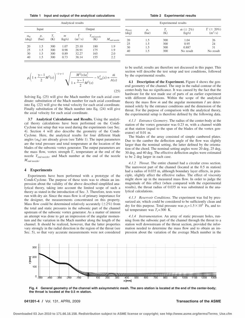
�t�1 +� − 1

2M2�x��−1/�−1� M2�x�at

2

1 +� − 1

2M2�x�

− Vtan2 �x� =

m

A�x�

�25�Solving Eq. �25� will give the Mach number for each axial coor-dinate: substitution of the Mach number for each axial coordinateinto Eq. �22� will give the total velocity for each axial coordinate.Finally substitution of the Mach number into Eq. �24� will givethe axial velocity for each axial coordinate.

3.7 Analytical Calculations and Results. Using the analyti-cal theory calculations have been performed on the Condi-Cyclone test setup that was used during the experiments �see Sec.4�. Section 4 will also describe the geometry of the Condi-Cyclone. Here, the analytical results for four different bladeangles ��bl� are already given �see Table 1�. The input parametersare the total pressure and total temperature at the location of theblades of the subsonic vortex generator. The output parameters arethe mass flow, vortex strength �, temperature at the end of thenozzle Tend nozzle, and Mach number at the end of the nozzleMend nozzle.

4 ExperimentsExperiments have been performed with a prototype of the

Condi-Cyclone. The purpose of these tests was to obtain an im-pression about the validity of the above described simplified ana-lytical theory, taking into account the limited scope of such atheory as stated in the introduction of Sec. 3. Therefore, tests wererun with dry air. Since the mass flow is of primary importance forthe designer, the measurements concentrated on this property.Mass flow could be determined relatively accurately ��2%� fromthe total and static pressures in the subsonic part of the channelupstream of the subsonic vortex generator. As a matter of interestan attempt was done to get an impression of the angular momen-tum and the variation in the Mach number along the length of thechannel. It should be realized, however, that the latter propertiesvary strongly in the radial direction in the region of the throat �seeSec. 5�, so that very accurate measurements were not considered

to be useful; results are therefore not discussed in this paper. Thissection will describe the test setup and test conditions, followedby the experimental results.

4.1 Description of the Experiment. Figure 4 shows the gen-eral geometry of the channel. The step in the radial contour of thecenter-body has no significance. It was caused by the fact that thehardware for the test made use of parts of an earlier experimentwith different dimensions. Within the scope of the analyticaltheory the mass flow m and the angular momentum I are deter-mined solely by the entrance conditions and the dimension of thethroat. For the purpose of comparison with the analytical theory,the experimental setup is therefore defined by the following data.

4.1.1 Entrance Geometry. The radius of the center-body at thestation of the vortex generator was 0.23 m, with a channel widthat that station �equal to the span of the blades of the vortex gen-erator� of 0.01 m.

The blades of the array consisted of simple cambered plates.Due to the camber the deflection angle of the flow was slightlylarger than the nominal setting, the latter defined by the orienta-tion of the chord. The nominal setting angles were 20 deg, 25 deg,30 deg, and 40 deg. The effective deflection angles were estimatedto be 2 deg larger in each case.

4.1.2 Throat. The entire channel had a circular cross section.The narrowest part of the channel �located at the 0.5 m station�had a radius of 0.035 m, although boundary layer effects, in prin-ciple, slightly affect the effective radius. The effect of viscositymight show up in the measured mass flow. In order to judge themagnitude of this effect �when compared with the experimentalresults�, the throat radius of 0.035 m was substituted in the ana-lytical calculations.

4.1.3 Reservoir Conditions. The experiment was fed by pres-surized air, which could be considered to be sufficiently clean anddry for this purpose. Total pressure was pt=1.5�105 Pa, and to-tal temperature was Tt=300 K.

4.1.4 Instrumentation. An array of static pressure holes, run-ning from the subsonic part of the channel through the throat to astation well downstream of the throat section, provided the infor-mation needed to determine the mass flow and to obtain an im-pression about the variation of the average Mach number in the

Table 1 Input and output of the analytical calculations

Analytical results

Input Output

�bl�deg�

pt�bar�

Tt�K�

m�kg/s�

��m2 /s�

Tend nozzle�K� Mend nozzle

20 1.5 300 1.07 25.10 180 1.925 1.5 300 0.98 28.91 175 1.930 1.5 300 0.89 32.27 165 2.040 1.5 300 0.73 38.14 155 2.2

Table 2 Experimental results

Experimental results

�SVG�deg�

pt�bar�

Tt�K�

m �� 2%��kg/s�

� �� 20%��m2 /s�

20 1.5 300 1.04 2625 1.5 300 0.95 2430 1.5 300 0.887 3140 1.5 300 No result No result

Fig. 4 General geometry of the channel with axisymmetric mesh. The zero station is located at the end of the center-body;the throat is located at the 0.5 m station.



channel.A crude check on the magnitude of the swirl was made by

mounting a three-hole pressure tube in the widest part of the chan-nel near the aft end of the central body. This pitot tube could berotated in such a way that it was roughly aligned with the flowdirection. From this device the flow angle � was derived on themean radius of this particular station.

The measured vortex strength was expressed in terms of thecirculation � defined as

� = 2rVtan = 2rblMblabl sin �bl �26�The expected accuracy is not more than 20% due to the uncertain-ties in the measurement techniques. On account of the quasi-one-dimensional assumption underlying the analytical theory, the cir-culation is related to the angular momentum I by the expression

I =m

2� �27�

4.2 Experimental Results. Experiments with the Condi-Cyclone have been performed at the Stork Product EngineeringTM620-Air/Water test facility �2,3�. The results of the test for

different blade angle deflections are given in Table 2. With in-creasing blade deflection angle and thus with increasing vortexstrength, the mass flow through the nozzle decreases. At the high-est blade deflection angle �40 deg� the test setup started to vibrateheavily, and the mass flow was severely limited. Because of thevibrations the test was aborted and therefore no results are avail-able for this blade deflection angle. Either vortex breakdown orthe stalling of the blades of the SVG is thought to be the probablecause for these vibrations.

5 Euler Numerical SimulationThe Euler numerical simulation �4� was performed using the

geometry of the test channel. The purpose was to obtain informa-tion on the radial variations in the flow, which may be expected tohave occurred during the experiment. Another goal was to checkwhether local shocks on the tail of the center-body could haveoccurred, thus causing the breakdown of the experiment with thelargest vane angles. For this specific purpose the Euler numericalsimulation was considered adequate.

5.1 Mesh Generation. Meshes have been generated to per-form dry air Euler numerical simulations for the Condi-Cyclone

Fig. 5 Axisymmetric mesh; zoomed in at the end of the center-body

Fig. 6 Tangential velocity „horizontal axis… as a function of radial distance „vertical axis…for several stations



SVG with various blade deflection angles. An axisymmetric meshwas used �starting just downstream of the static array of bladesand running through the throat until well downstream of thethroat�.

Because an axisymmetric flow is assumed, it was only neces-sary to generate a two-dimensional mesh. The mesh is a structuredH-type mesh with dimensions of 124�24 cells for the first block�running from just downstream of the blades until halfway of thecenter-body�. The remainder of the channel consisted of fourblocks of each 108�24 cells. The distribution of mesh points hasbeen chosen in such a way that the width of the cells approximatesthe height of the cells and that a refinement can be found at theend of the center-body and along the nozzle axis of symmetry �seeFig. 5�. Numerical simulations have also been performed withfiner meshes. However mesh convergence was reached, and there-fore results for these finer meshes have been omitted. The inflowboundary conditions, just downstream of the swirl vanes, werechosen to correspond to the flow conditions determined by theanalytical calculations.

5.2 Results of Numerical Analysis. The main findings of thenumerical simulations are the following: The vortex causes theflow to reach sonic conditions well upstream of the nozzle throat

in the region of the tail of the center-body. In the nozzle throat theaxial velocity is equal to the local speed of sound, as predicted bythe analytical theory. In the nozzle a vortex structure is found witha solid body rotation at the axis of symmetry and a “1 over r”behavior toward the nozzle wall �see Fig. 6�. A severe pressuredrop is present in the region of the solid body rotation.

With increasing blade deflection angle the mass flow decreases,the vortex strength increases, a higher Mach number at the end ofthe nozzle is achieved, and a slightly larger temperature drop oc-curs �see Table 3�. With increasing blade deflection angles thesolid body rotation region expands, the supersonic region at theend of the center-body moves upstream, and the effective crosssection of the channel decreases. At the highest vane angle of 40deg a flow disturbance at the very end of the center-body wasclear �see Fig. 7�, showing up as a region of back-flow near thecenter-line and possibly involving a small shock. It was thereforerecommended to use in later configurations center-bodies with apluglike tail shape.

6 Comparison of Analytical, Numerical, and Experi-mental Results

The results of the analytical theory, experiments, and numericalsimulation as explained in Secs. 3–5 will be compared.

6.1 Mass Flow and Vortex Strength. The mass flow andvortex strength as predicted by the analytical theory, calculated bythe numerical simulation, and measured during the experimentsare plotted as a function of the blade deflection angle in Fig. 8. Ascan be seen from this figure, the results correspond reasonablywell, especially when taking into account that the experimentallyobtained values for the vortex strength have an accuracy of only20%. The measured mass flow does not seem to be affected ap-preciably by viscosity effects.

6.2 Axial Velocity, Temperature, and Mach Number. Boththe analytical results and the numerical results show that the total

Table 3 Input and output of the Euler numerical simulation

Numerical results

Input Output

�SVG�deg� Mbl

pt�bar�

Tt�K�

m�kg/s�

��m2 /s�

Tend nozzle�K� Mend nozzle

20 0.14 1.5 300 1.12 23.31 186 1.7525 0.13 1.5 300 1.02 27.37 180 1.8030 0.13 1.5 300 0.91 32.68 174 1.8540 0.12 1.5 300 0.69 39.07 168 1.95

Fig. 7 Calculated back-flow at the end of the center-body



Mach number becomes supersonic well before the throat, just up-stream of the end of the center-body. Both results also show thatthe axial velocity in the throat is equal to the local speed of sound.The Mach number and temperature at the end of the nozzle �sta-tion 1.3 m downstream of the center-body� as predicted by theanalytical theory and calculated by the numerical simulation areplotted in Fig. 9.

7 ConclusionsThe analytical theory developed to describe a vortex flow

through a Laval nozzle predicts that the axial velocity in the throatwill be equal to the local speed of sound and that the total velocitywill be larger than the local speed of sound. The total velocity willreach M =1 upstream of the throat. Furthermore, the theory pre-dicts that the mass flow through the nozzle depends on the condi-tions in the throat and also on the vortex strength. The predictionsfrom a simplified analytical theory have been compared with theresults of a numerical simulation and experiments and correspondvery well.

8 EpilogueAfter some modifications were applied to the Condi-Cyclone �a

change in the end of the center-body and a redesign of the static

array of blades�, the concept performed very well during the ex-periments. The Condi-Cyclone concept has been patented byStork Product Engineering and has been further developed byTwister BV to make the technology commercially available to thewider industry. A Twister demonstration unit has been operationalin Nigeria since early 2001, successfully performing water andhydrocarbon separation, while confirming the ability of Twister torun virtually without supporting systems �Twister BV�. Earlierunits have been in operation in the Netherlands in Zuiderveen enBarendrecht since 1997 �5�.

References�1� Knott, T., 2000, “Twist in the Tale,” Offshore Engineer, http://

www.oilonline.com/news/features/oe/20000701.Twist_in.67.asp.�2� Mertens, S., 1999, “Test Report: Subsonic Vortex Generation �20 & 40 De-

grees Turbine Ring�,” Stork Product Engineering, Amsterdam, The Nether-lands, Technical Report No. SPE-CON-RP-102 �1/0�.

�3� Mertens, S., 1999, “Test report: Subsonic Vortex Generation �25 & 30 DegreesTurbine Ring�,” Stork Product Engineering, Amsterdam, The Netherlands,Technical Report No. SPE-CON-RP-113 �1/0�.

�4� Schoones, M. M. J., and Van Holten, Th., 1999, “Euler Numerical Simulationof Channel Flow With a Superimposed Vortex,” Faculty of Aerospace Engi-neering, Delft University of Technology, The Netherlands, Technical ReportNo. FM&P-99.001.

�5� Twister, B. V., http://www.twisterbv.com/

Fig. 8 Mass flow and vortex strength as a function of the blade deflection angle

Fig. 9 Temperature and Mach number at the end of the nozzle as a function of the blade deflection angle



Mohsen Akbari1

Ph.D. CandidateMechatronic System Engineering,

School of Engineering Science,Simon Fraser University,

Surrey, BC, V3T 0A3, Canadae-mail: [email protected]

David SintonAssociate Professor

Department of Mechanical Engineering,University of Victoria,

Victoria, BC, V8W 2Y2, Canada

Majid BahramiAssistant Professor

Mem. ASMEMechatronic System Engineering,

School of Engineering Science,Simon Fraser University,

Surrey, BC, V3T 0A3, Canada

Pressure Drop in RectangularMicrochannels as Compared WithTheory Based on Arbitrary CrossSectionPressure driven liquid flow through rectangular cross-section microchannels is investi-gated experimentally. Polydimethylsiloxane microchannels are fabricated using soft li-thography. Pressure drop data are used to characterize the friction factor over a range ofaspect ratios from 0.13 to 0.76 and Reynolds number from 1 to 35 with distilled water asworking fluid. Results are compared with the general model developed to predict the fullydeveloped pressure drop in arbitrary cross-section microchannels. Using available theo-ries, effects of different losses, such as developing region, minor flow contraction andexpansion, and streaming potential on the measured pressure drop, are investigated.Experimental results compare well with the theory based on the presure drop in channelsof arbitrary cross section. �DOI: 10.1115/1.3077143�

1 IntroductionAdvances in microfabrication make it possible to build micro-

channels with micrometer dimensions. Micro- and minichannelsshow potential and have been incorporated in a wide variety ofunique, compact, and efficient cooling applications in microelec-tronic devices �1�. These microheat exchangers or heat sinks fea-ture extremely high heat transfer surface area per unit volumeratios, high heat transfer coefficients, and low thermal resistances.In biological and life sciences, microchannels are used widely foranalyzing biological materials such as proteins, DNA, cells, em-bryos, and chemical reagents �2�. Various microsystems, such asmicroheat sinks, microbiochips, microreactors, and micronozzleshave been developed in recent years �3–6�. Since microchannelsare usually integrated into these microsystems, it is important todetermine the characteristics of the fluid flow in microchannels forbetter design of various microflow devices.

In parallel to the recent advances in microfluidic devices, mi-crofabrication techniques have evolved. Some of the importantfabrication techniques include lithography �soft and photolithog-raphy�, lamination, injection molding, hot embossing, laser micro-machining, and electrochemical or ultrasonic technologies�2,7–10�. Together with new methods of fabrication, it is possibleto exploit certain fundamental differences between the physicalproperties of fluids moving in large channels and those travelingthrough micrometer-scale channels �2�. In recent years, a largenumber of papers have reported pressure drop data for laminarfully developed flow of liquids in microchannels with variouscross sections �11–32�. Rectangular cross sections have been ex-tensively studied as they are employed in many applications�11–16�. However, published results are often inconsistent. Someauthors reported a huge deviation from the conventional theoriesand attributed it to an early onset of laminar to turbulent flowtransition or surface phenomena such as surface roughness, elec-trokinetic forces, viscous heating effects, and microcirculationnear the wall �12–26�.

Jiang et al. �28� conducted an experimental investigation of

water flow through different microchannel cross sections includ-ing circular, rectangular, trapezoidal, and triangular. The hydraulicdiameter of microchannels varied from 8 �m to 42 �m. Theycollected experimental data with the Reynolds number rangingfrom 0.1 to 2, and concluded that there was less influence of thecross-sectional shape on the microflow in the microchannel andthat the experimental data agreed well with the prediction of theconventional theory. Baviere et al. �29� performed an experimen-tal study on the water flow through smooth rectangular micro-channels. Their channels were made of a silicon engraved sub-strate anodically bonded to a Pyrex cover. Their results showedthat in smooth microchannels, the friction law is correctly pre-dicted by conventional theories. Judy et al. �15� and Bucci et al.�30� showed that their experimental results were in good agree-ment with conventional theories in the laminar regime. Also Wuand Cheng �31�, Liu and Garimella �32�, and Gao et al. �33�reported good agreement between experimental data with conven-tional theories.

Low Reynolds numbers characterize many microscale liquidflows �34�. Hence, nonlinear terms in the Navier–Stokes equationdisappear for fully developed flow, resulting in Poisson’s equation

�2u =1

�

dp

dz, u = 0 on � �1�

where u is the fluid velocity, z is the flow direction, and � is theperimeter of the channel. Exact solution for Eq. �1� in rectangularcross-section channels can be found in fluid mechanics textbookssuch as Ref. �35�. The original analytical solution for the meanvelocity in rectangular channels is in the form of a series, but ithas been shown that using the first term of the series results inerrors less than 0.7%.

Recently, Bahrami et al. �1,36� developed a general model forprediction of pressure drop in microchannels of arbitrary crosssection. Using the analytical solution of elliptical duct and theconcept of Saint-Venant principal in torsion �37�, they showed thatthe Poiseuille number, f Re�A, is a function of the polar momentof inertia, IP, area, A, and perimeter of the cross section of thechannel, �. Their model showed good agreement with experimen-tal and numerical data for a wide variety of channel cross sectionssuch as rectangular, trapezoidal, triangular, circular, and moonshaped.


JOURNAL OF FLUIDS ENGINEERING. Manuscript received June 11, 2008; final manuscriptreceived December 5, 2008; published online March 6, 2009. Assoc. Editor: JamesA. Liburdy. Paper presented at the ECI International Conference on Heat Transferand Fluid Flow in Microscale III, Whistler, BC, Canada, September 21–26, 2008.



However, they �1,36� did not perform any experiment to verifythis model, thus they could not investigate all issues and effects ofdifferent parameters. As a result the goal of the present work is toindependently validate the general model of Bahrami et al. �1,36�.Moreover, effects of different parameters, including microchanneldimensions, minor and developing region losses, viscous heating,electroviscous phenomena, and channel deformation on the mea-sured pressure drop, have been discussed. By successfully validat-ing the model, it will be used in more complicated channel geom-etries such as variable cross-section microchannels.

2 TheorySelection of the characteristic length is an arbitrary choice and

will not affect the final solution. However, an appropriate lengthscale leads to more consistent results, especially when a generalcross section is considered. A circular duct is fully described withits diameter, thus the obvious length scale is the diameter �orradius�. For noncircular cross sections, the selection is not asclear; many textbooks and researchers have conventionally chosenthe hydraulic diameter as the characteristic length. Yovanovich�38� introduced the square root of area as a characteristic lengthscale for heat conduction and convection problems. Later, Muzy-chka and Yovanovich �39� proposed the use of �A for the fullydeveloped flow in noncircular ducts. Bahrami et al. �1,37� showedthat the square root of area appears in the solution of fully devel-oped flow in noncircular ducts. They also compared both Dh and�A and observed that using �A as the characteristic length scaleresults in similar trends in Poiseuille number for microchannelswith a wide variety of cross sections. Therefore, in this study, �Ais selected consistently as the length scale throughout the analysis.

According to the model of Bahrami et al. �1�, pressure drop oflaminar fully developed flow in arbitrary cross-section microchan-nels can be obtained from

�P = 16�2�QIp� L

A2 �2�

where Ip� = Ip /A is the specific polar momentum of inertia of the

microchannel cross section, �=4�W+H� is the microchannelcross-section perimeter, L is the fully developed length, and Q isthe the volumetric flow rate. Substituting for the geometrical pa-rameters in Eq. �2� for microchannels of rectangular cross sectionand the definition of the Poiseuille number yields �1�

f Re�A =4�2�1 + �2�

3��1 + ��3�

As can be seen the only parameter effects the Poiseuille numberin rectangular channels is the cross-section aspect ratio, consistentwith previous works �35,40�. For rectangular microchannels, twoasymptotes can be recognized, i.e., very narrow rectangular andsquare channels

f Re�A =4�2

3��; � → 0

f Re�A = 13.16; � = 1 �4�

3 Experimental Setup

3.1 Chemicals and Materials. De-ionized water was used asthe testing liquid. SU-8 photoresist �Microchem, Newton, MA�and diacetone-alcohol developer solution �Sigma-Aldrich, St.Louis, MO� were used in the making of the positive relief mastersby the procedure outlined below. Polydimethylsiloxane �PDMS�casts were prepared by thoroughly mixing the base and curingagent at a 10:1 ratio as per the manufacturer’s instructions for theSylgard 184 silicon elastomer kit �Dow Corning, Midland, MI�.Caution was used to avoid contact between the liquid PDMS andlatex rubber �gloves�, as this was found to inhibit curing �41�.

3.2 Microfabrication. The PDMS/PDMS microchannelsused in this study have been manufactured using the soft lithog-raphy technique �42� described by Erickson et al. �41�. A sche-matic of the process is provided in Fig. 1. Photomasks were de-signed by AUTOCAD software2 and printed with a 3500DPI printer�Island Graphics Ltd., Victoria, BC, Canada�. Masters containingthe desired microchannel pattern have been made by spin coatingof SU-8 negative photoresist on a glass slide to the desired thick-ness. The photoresist film was then hardened through a two-stagedirect contact pre-exposure bake procedure �65°C for 5 min and95°C for 30 min� and exposed to UV light for 100 s through themask containing the channel pattern. A two-stage postexposurebake procedure �65°C for 5 min and 95°C for 30 min� was thenused to enhance cross linking in the exposed portion of the film.The slide was then placed in quiescent developer solution for 10min to dissolve the unexposed photoresist, leaving a positive reliefcontaining the microchannel pattern.

Liquid PDMS was then poured over the master and exposed tovacuum condition �1 h� to extract all the bubbles in it and cured at85°C for 15–20 min yielding a negative cast of the microchannelpattern. An enclosed microchannel was then formed by bondingthe PDMS cast with another piece of PDMS via plasma treatment.

Five microchannels were made with a range of aspect ratios,0.13��0.76, and tested in this study. Dimensions of the micro-channels are shown in Table 1. The channels’ names in the tableindicate the channel material, cross-sectional shape, and the aspectratio �i.e., PPR-0.13 corresponds to the PDMS/PDMS chip withrectangular cross section and the aspect ratio of 0.13�. As can beseen, channels were designed long enough so that fully developedflow is dominant. Since the microchannel dimensions have a ma-jor effect on the friction factor calculation �13,15,33�, a destruc-tive careful measurement was performed after the experiments.Channels were cut carefully at three random cross sections. Thecutting lines were perpendicular to the channel to ensure a 90 degviewing angle. Dimensions of the channel were measured by animage processing method. To do so, a Leica DMI 6000B �LeicaMicrosystems, Richmond Hill, ON, Canada� microscope with a10�, 0.4 N.A. objective was used. Images of the channel cross

2www.usa.autodesk.com.

Fig. 1 Schematic of the soft lithography technique



section were captured by a high resolution high sensitivity CCDcamera �Hamamatsu Orca AG, NJ� and imported into a photoediting software, ADOBE PHOTOSHOP 8.0. Dimensions of the chan-nel were then measured by pixel counting. Size of each pixel wascalibrated using a known dimension provided by the microscopeimage acquisition software. Accuracy of this method was found tobe �3.6 �m. Due to the microfabrication process, the microchan-nel cross section has some deviations from the rectangular shape.Height and width measurements were conducted at different ran-dom positions for each cross section and the average value wasdetermined. This measurement was also performed at severalcross sections. Mean values are reported in Table 1. It was ob-served that both microchannel depth and width were differentfrom the expected values in the fabrication process. From ourmeasurements, channel height, and width deviated less than 4%and 3% from the designed sizes, respectively. Since smooth sur-faces were observed by the image processing technique describedabove, the roughness of the channels was estimated to be less thanthe accuracy of the image processing method. Hence, the relativechannel roughness �channel roughness/channel length scale� wasfound to be less than 3%. As a result the effect of roughness on thepressure drop of the fully developed flow can be neglected �27�.

3.3 Experimental Procedure. An open loop syringe pumpsystem, as illustrated in Fig. 2, was designed for this work. Asyringe pump �Harvard Apparatus, QC, Canada� provided con-stant flow rate with �0.5% accuracy. A range of Reynolds num-bers was covered by changing the volumetric flow rate from40 �l /min to 240 �l /min. Water was forced to flow through asubmicron filter �Aktreingeselchaf Co., Germany� before enteringthe channel. To measure the pressure drop, a gauge pressure trans-ducer �Omega Inc., Laval, QC, Canada� was fixed at the channelinlet while the channel outlet was opened to the atmosphere. Te-flon tubing �Scientific Products And Equipment, North York, ON,Canada� was employed to connect the pressure transducer to thesyringe pump and the microchannel. Measured pressure was thenmonitored and recorded with a computerized data acquisition sys-

tem �LABVIEW 8.5, National Instruments, USA3�. The flow wasconsidered to have reached a steady state condition when the read-ings of the pressure drop did not change with time. For a givenchannel, the measurement of pressure drop was repeated threetimes for each flow rate. An arithmetic averaging method �43� wasperformed to determine the final results.

4 Analysis of Experimental DataReynolds number was calculated knowing the volumetric flow

rate, Q, and the cross-sectional area, A, from

Re�A =Q

��A�5�

Viscous dissipation effect was neglected since the dimension-less number 4 Ec�L�f Re�A� /Re�A=0.006 is much smaller than1. The value of �Tref=1°C was used to calculate the Eckert num-ber, Ec, for water as a working fluid �26�. Hence, the properties ofthe water was assumed to be constant.

Total measured pressure drop during the experiment, �Pmeasuredis

�Pmeasured = �Pc + �Pin + �PD + �PFD + �Pex + 2�Pb + �Pev

�6�

where �Pc is the pressure loss due to the flow in the connectingtubes, �Pin and �Pex are the inlet and exit losses, �PD is thedeveloping region loss, �PFD is the pressure drop in the fullydeveloped region, �Pb is the pressure drop due to 90 deg bends,and �Pev is the pressure drop corresponds to the electroviscouseffect. Since fully developed pressure drop is the focus of thisstudy, right hand side losses except �PFD must be subtracted fromthe measured pressure drop.

4.1 Connecting Tube Pressure Loss, �Pc. The connectingtube pressure drop includes the losses due to all fittings and thecapillary tube from the transducer to the microchannel inlet. Wemeasured this loss directly at each flow rate when there was nomicrochannel at the end of the tubing. The measurements werecarefully conducted with the conditions identical to the case whena microchannel was added to the end of the connecting tube toavoid the effects of hydrostatic pressure.

4.2 Developing Region, �PD. Since the viscous boundarylayer inherently grows faster in microchannels than in macros-cales, the developing region in most cases is negligible. There arefew references that can be found in literature, in which the effectof inlet region was considered �40,44,45�. Phillips �44� showedthat the length of the hydrodynamic developing region, LD, de-pends on the aspect ratio of rectangular cross-section microchan-nels; the higher the aspect ratio, the longer the developing length.Maximum value of LD can be obtained from Eq. �7�

LD =4�

�1 + ��2

Q

��7�

This equation shows that the developing length depends on theflow rate and the channel aspect ratio. The higher the aspect ratioand/or flow rate, the higher the developing length. Ratio of themaximum developing length over the total length of the micro-channel is listed in Table 1 for different channels. Obviously thislength occurs in the maximum flow rate. Pressure drop associatedwith the entrance region after changing the length scale to �A is�46�

�PD =�f Re�A��Q�

2A�ALD + K

Q2

2A2 �8�

where K=0.6796+1.2197�+3.3089�2−9.5921�3+8.9089�4

3www.ni.com.

Table 1 Dimensions of the fabricated microchannels

ChannelWidth, 2W

��m�Depth, 2H

��m�Length, L

�mm� �=H /W LD,max /L�%�

PPR-0.13 780 110 50 0.13 3.47PPR-0.17 581 101 50 0.17 4.03PPR-0.4 480 192 58.8 0.4 5.55PPR-0.6 189 113 55.5 0.6 6.75PPR-0.76 134 103 50 0.76 7.86

Fig. 2 Schematic of the test section



−2.9959�5.In Eq. �8�, f Re�A was calculated based on the measured pres-

sure drop. Table 2 lists the relative pressure loss of the developingregion with respect to the measured pressure drop. As can be seen,the values are small, less than 0.3%, and can be neglected for therange of Reynolds numbers studied in this work �1�Re�A�35�.For the higher Reynolds numbers �Re�100�, the developing pres-sure drop, �PD, was found to be less than 2% of the fully devel-oped pressure drop obtained from Eq. �3�.

4.3 Minor Losses, �Pmin. Other pressure losses associatedwith the measured pressure drop are inlet, exit, and bend losses.These losses are usually obtained from the traditional relation-ships used in macroscale �15,44,46,47�. Phillips �44� showed thatthe minor pressure losses can be obtained from

�Pmin = �Pin + �Pex + 2�Pb =Q2

2A�Kc + Ke + 2Kb� A

At2

�9�

where A and At are the channel and connecting tube cross-sectional areas, respectively. Kb is the loss coefficient for thebend, and Kc and Ke represent the contraction and expansion losscoefficients due to area changes. Phillips �44� recommended Kb tobe approximately 1.2 for a 90 deg bend. Assuming equal cross-sectional areas for the channel and connecting tubes and alsomaximum possible values for Kc and Ke �48�, relative minorlosses with respect to the measured pressure drop are listed inTable 3. As can be seen, these losses are negligible compared withthe measured pressure drop. For higher Reynolds numbers �Re�100�, minor pressure drop, �Pmin, was found to be less than 5%of the fully developed pressure drop obtained from Eq. �3�.

4.4 Electroviscous Effect, �Pev. When a liquid is forcedthrough a narrow channel under an applied pressure gradient, thecounterions in the diffusive layer of EDL �electric double layer�are moving toward the downstream end and a potential gradient isinduced in the flow �49�. This so called streaming potential acts to

drive the counterions in the diffuse layer of the EDL to move inthe direction opposite to the pressure-driven flow. The overall re-sult is a reduced flow rate for a constant pressure gradient orincrease in pressure drop for a given flow rate. This phenomenon,which gives the appearance of an increased viscosity, �a, is calledthe electroviscous effect �50�. The ratio of this apparent viscosityto the actual fluid viscosity for circular cross-section capillariescan be found from �50�

�a

�� 1 +

32�

bD2�eo2 �10�

where D is the capillary diameter, � is the fluid viscosity, b is theliquid electrical conductivity, and a is the radius of the capillary.�eo=�0�r� /� is the electro-osmotic mobility, where �0=8.854�10−12 C2 V−1 m−1 is the permittivity of vacuum, �r=78.3 is therelative permittivity for water at 25°C �49�, and � is the zetapotential of the surface. Approximating the rectangular cross-section microchannel with a capillary of the same cross-sectionalarea, b=5.6�10−6 S m−1 �51� and �eo=5.9�10−8 m2 V−1 s−1

�52� for PDMS, value of �a /� was found to be less than 1.03 forthe channel sizes in this study.

4.5 Effect of Channel Deformation Under Pressure-DrivenFlow. Effect of channel deformation becomes important since itcan change the microchannel cross-sectional area and as a resultthe pressure drop. In all equations used in Secs. 1–3, we assumedthat the channel cross section did not change under pressure-driven flow. Few works have discussed the importance of bulkdeformation in rectangular microchannels. Holden et al. �53� mea-sured the PDMS bulk deformation under high pressure drops��1 bar� using the change in fluorescence intensity. Gervais et al.�54� studied the elastic deformation of PDMS microchannels un-der imposed flow rates. They demonstrated that the channel de-formation can effect the the laminar flow profile and pressuredistribution within the channels with low aspect ratios and highpressure drops. In a bulged microchannel, measured pressure dropno longer changes linearly with the flow rate �53�. This is becausethe microchannel cross section varies due to deformation, and fora constant flow rate, pressure drop changes. Figure 3 shows thevariation in the channel pressure drop with flow rate for presentwork. Experimental results properly follow the linear behavior oftheoretical profiles. Thus one can conclude that the channel defor-mation has negligible effect on the results in this work. However,a careful experimental and theoretical investigation is required tostudy the effect of the channel deformation on the pressure drop ofmoderate and high aspect ratio rectangular cross-section micro-channels.

4.6 Uncertainty Analysis. A careful analysis of the experi-mental uncertainty in this study is critical to the interpretation ofexperimental data of Poiseuille number, Po, and exploration ofdeviations from the macroscale theory. Neglecting the developingregion, minor losses, electroviscous effects, and considering thatthe channel deformation is not significant, the experimental Poi-seuille number can be obtained from

Poexp =4

�Q�A2�A

L��PFD �11�

where �PFD=�Pmeasured−�Pc. The uncertainty associated withPoexp based on the measured variables, and the method providedin Ref. �43� is then given by

�Poexp

Poexp= ��P

�P2

+ ��L

L2

+ ��

�2

+25

4��A

A2

+ ��Q

Q21/2

�12�

where � values indicate uncertainty associated with each variableas subscribed, �A=4��H�W�2+ �W�H�2�1/2 and ��=4��W

2 +�H2 �1/2

�see Appendix for details of calculations�. In this equation we

Table 2 Ratio of the developing region pressure drop over themeasured pressure drop of the microchannel

�PD /�Pmeasured�%�

Q��l /min� �=0.13 �=0.17 �=0.4 �=0.6 �=0.76

40 0.01 0.01 0.04 0.03 0.0460 0.01 0.02 0.03 0.04 0.0680 0.01 0.02 0.04 0.06 0.08100 0.02 0.01 0.06 0.07 0.10120 0.02 0.02 0.06 0.08 0.11240 0.03 0.05 0.10 0.20 0.24

Table 3 Ratio of the minor pressure loss over the measuredpressure drop of the microchannel

�Pmin /�Pmeasured�%�

Q��l /min� �=0.13 �=0.17 �=0.4 �=0.6 �=0.76

40 0.04 0.04 0.12 0.09 0.1160 0.05 0.07 0.10 0.13 0.1780 0.07 0.10 0.14 0.17 0.23100 0.08 0.07 0.21 0.22 0.28120 0.09 0.10 0.19 0.25 0.35240 0.16 0.24 0.35 0.51 0.70



assumed that the fluid properties remained constant. Equation �12�shows that the channel dimensions play an important role in de-termination of uncertainty by effecting three terms. Also for smallReynolds numbers, the accuracy of the flow rate becomes moresignificant. The uncertainty in the measurement of each parameteris listed in Table 4. Using Eq. �12� minimum uncertainties for thesamples of PPR-0.13, PPR-0.17, PPR-0.4, PPR-0.6, and PPR-0.76are 8.7%, 9.3%, 8.9%, 9.3%, and 11.1%, respectively.

5 Results and DiscussionFigures 4 and 5 show the comparison between friction factor

obtained from Eq. �3�, the solid line, and experimental data fortwo typical samples of PPR-0.13 and PPR-0.76, respectively. Asshown, the trend and the values of experimental data are wellpredicted by the theoretical model. Consistent with the laminarflow in channels friction factor decreases with the Reynolds num-ber.

Variation in the Poiseuille number, f Re�A, with the Reynoldsnumber for different channels is shown in Fig. 6. Experimentaldata are normalized by the analytical model obtained from Eq. �3�.The solid line shows the analytical model. From Eq. �3�, it is clearthat the Poiseuille number does not depend on the Reynolds num-ber and it only varies with the aspect ratio of the channel crosssection. The same trend can be observed in the experimental data.Large deviations from this trend in the very low Reynolds num-bers attributed to the large uncertainties occur due to small flowrates and pressure drops. The Reynolds number can be a result ofthe small cross-sectional area and/or flow rate, with both param-eters increasing the uncertainty in the value of the Poiseuille num-ber, see Eq. �12�. As can be seen, most of the experimental pointsfall within �10% bounds of the analytical model.

Another comparison of the present experimental work with ana-lytical model is illustrated in Fig. 7. Since the Poiseuille number,f Re�A, remains constant for the laminar regime as the Reynoldsnumber varies, the experimental data for each set were averagedover the laminar region. The �10% bounds of the model are alsoshown in the plot to better demonstrate the agreement between thedata and the model.

As shown in Eq. �3�, the Poiseuille number, f Re�A, is only afunction of the aspect ratio, which is a geometrical parameter.This dependency is plotted in Fig. 8. Averaged values over thestudied range of the Reynolds number were used in this plot. Itcan be observed that for smaller aspect ratios, the Poiseuille num-ber, f Re�A, increases sharply. To better show the trend of theanalytical model, two asymptotes of very narrow and square crosssections are also included in Fig. 8. As can be seen, when �→0,parallel plate, the Poiseuille number asymptotically approaches4�2 /3��.

Table 4 Uncertainty values for measured parameters

Parameter Uncertainty

�P �0.25% of full scaleL �0.02 mmW �3.6 �mH �3.6 �mQ �0.5%

Fig. 3 Channel pressure drop as a function of flow rate. Linesshow the theoretical prediction of pressure drop using Eq. „3…and symbols show the experimental data.

Fig. 4 Variation in friction factor with Reynolds number forsample no. PPR-0.13

Fig. 5 Variation in friction factor with Reynolds number forsample no. PPR-0.76



It is beneficial to compare the results of present work with theexisting data of rectangular microchannels. Data were collectedfrom the works of Wu and Cheng �31�, Lu and Garimella �32�,and Gao et al. �33�. As shown in Fig. 9, the collected data cover awide range of the aspect ratio for almost three decades. The solidline represents the analytical model of Bahrami et al. �1�. As canbe seen, the analytical model agrees well with the experimentaldata over the wide range of microchannel cross-section aspectratio.

6 Summary and ConclusionsThe general model developed by Bahrami et al. �1,36� was

experimentally validated for the case of rectangular cross-sectionmicrochannels. Frictional pressure drop measurements were con-ducted over a range of Reynolds numbers from 1 to 35 for rect-angular cross-section microchannels fabricated with soft lithogra-phy method in the aspect ratio range of 0.13��0.76. A carefulmeasurement of pressure drop and channel dimensions was con-

ducted, and the pressure drops due to the developing region, mi-nor losses, and electroviscous effect were estimated using avail-able models in literature. Channel deformation due to the pressureinside the microchannel was found to be negligible since the pres-sure drop changes linearly with the flow rate. Comparing the re-sults with the general theoretical model shows good agreementbetween the model and experimental data.

Uncertainty analysis showed that the measurement of channeldimensions and flow rate is critical in microscales. Here, micro-channel cross-section geometry was determined through process-ing high quality images of the channel cross section.

According to the analytical model and experimental data ofpresent work, the Poiseuille number, f Re�A, was found to be onlya function of microchannel geometry in the range of Reynoldsnumbers studied in this work. For rectangular cross sections, thechannel aspect ratio is the only parameter that affects the Poi-

Fig. 6 Variation in Poiseuille number, f Re�A, with Reynoldsnumber

Fig. 7 Comparison of experimental data of present work withanalytical model of Bahrami et al. †1‡

Fig. 8 Variation in Poiseuille number, f Re�A, with Reynoldsnumber

Fig. 9 Comparison between experimental data of presentstudy and previous works



seuille number. The analytical model employed in this work willbe applied to other channel geometries such as variable cross-section microchannels in our future work.

AcknowledgmentThe authors gratefully acknowledge the financial support of the

Natural Sciences and Engineering Research Council of Canada�NSERC�. Also they thank Dr. Viatcheslav Berejnov and Mr. AliK. Oskooi for their assistance.

NomenclatureA microchannel cross-sectional area, m2

At tubing cross-sectional area, m2

cp fluid specific heat, J /kg KEc Eckert number, W2 / �2cp�Tref�

f Fanning friction factorH channel half height, mIp polar momentum of inertia, m4

Ip� specific polar momentum of inertia, Ip /A2

Kb loss coefficient for bendKc flow contraction loss coefficientKe flow expansion loss coefficientL channel length, m

LD developing region length, mL�

dimensionless length L /�APo Poiseuille number, f Re�AQ volumetric flow rate, m3 /s

Re�A Reynolds number, Q /��AW channel half width, m

Greek�Pb bend pressure loss, Pa�Pc connecting tube pressure loss, Pa�PD developing region pressure loss, Pa�Pex exit pressure loss, Pa�PFD fully developed pressure loss, Pa�Pev pressure loss due to electroviscous effect, Pa�Pin inlet pressure loss, Pa

� channel aspect ratio, 2H /2W� channel cross-section perimeter, m� fluid viscosity, kg /m s

�a apparent viscosity, kg /m s�eo electro-osmotic mobility, m2 /V s

fluid density, kg /m3

b fluid electrical conductivity, S/m� uncertainty

Appendix: Uncertainty FormulationTo calculate the uncertainty associated with the experimental

measurements the following relation is used �43�:

�R = �� R

�xi�i21/2

�A1�

where �R is the uncertainty in results, R�x1 ,x2 , . . . ,xn�, and �i isthe uncertainty of the independent variable xi. If the results func-tion, R�x1 ,x2 , . . . ,xn�, takes the form of a product of the indepen-dent variables, R=x1

a1x2a2 , . . . ,xn

an, Eq. �A1� can be rewritten as

�R

R= �� ai

xi�i21/2

�A2�

The final form of the uncertainty of the Poiseuille number, Eq.�12�, is obtained using Eqs. �10� and �A2�.

To calculate the uncertainty of the channel cross section, A=4W�H, and perimeter, �=4�W+H�, Eq. �A1� is employed

�A = �� A

�W�W2

+ � �A

�H�H21/2

�A3�

�� = ��

�W�W2

+ � ��

�H�H21/2

�A4�

where �A /�W=4H, �A /�H=4W, �� /�W=4, and �� /�H=4.

References�1� Bahrami, M., Yovanovich, M. M., and Culham, J. R., 2006, “Pressure Drop of

Laminar, Fully Developed Flow in Microchannels of Arbitrary Cross-Section,”ASME J. Fluids Eng., 128, pp. 1036–1044.

�2� Whitesides, G. M., 2006, “The Origins and the Future of Microfluidics,” Na-ture �London�, 442, pp. 368–372.

�3� Grushka, E., McCormick, R. M., and Kirkland, J. J., 1989, “Effect of Tem-perature Gradients on the Efficiency of Capillary Zone Electrophoresis Sepa-rations,” Anal. Chem., 61, pp. 241–246.

�4� Fletcher, P. D. I., Haswell, S. J., Pombo-Villar, E., Warrington, B. H., Watts, P.,Wong, S., and Zhang, X., 2002, “Micro Reactors: Principles and Applicationsin Synthesis,” Tetrahedron, 58, pp. 4735–4757.

�5� DeWitt, S., 1999, “Microreactors for Chemical Synthesis,” Curr. Opin. Chem.Biol., 3�3�, pp. 350–356.

�6� Miyake, R., Lammerink, S. J., Elwenspoek, M., and Fluitman, H. J., 1993,“Micro Mixer With Fast Diffusion,” MEMS ’93, Fort Lauderdale, FL, pp.248–253.

�7� Weigl, B. H., Bardell, R. L., and Cabrera, C. R., 2003, “Lab-on-a-Chip forDrug Development,” Adv. Drug Delivery Rev., 55, pp. 349–377.

�8� Becker, H., and Locascio, L. E., 2002, “Polymer Microfluidic Devices,” Tal-anta, 56, pp. 267–287.

�9� Chovan, T., and Guttman, A., 2002, “Microfabricated Devices in Biotechnol-ogy and Biochemical Processing,” Trends Biotechnol., 20�3�, pp. 116–122.

�10� Ehrfeld, W., 2003, “Electrochemistry and Microsystems,” Electrochim. Acta,48, pp. 2857–2868.

�11� Bayraktar, T., and Pidugu, S. B., 2006, “Characterization of Liquid Flows inMicrofluidic Systems,” Int. J. Heat Mass Transfer, 49, pp. 815–824.

�12� Peng, X. F., Peterson, G. P., and Wang, B. X., 1994, “Frictional Flow Charac-teristics of Water Flowing Through Rectangular Microchannels,” Exp. HeatTransfer, 7, pp. 249–64.

�13� Xu, B., Ooi, K. T., and Wong, N. T., 2000, “Experimental Investigation ofFlow Friction for Liquid Flow in Microchannels,” Int. Commun. Heat MassTransfer, 27, pp. 1165–1176.

�14� Ren, C. L., and Li, D., 2004, “Electroviscous Effects on Pressure-Driven Flowof Dilute Electrolyte Solutions in Small Microchannels,” J. Colloid InterfaceSci., 274, pp. 319–330.

�15� Judy, J., Maynes, D., and Webb, B. W., 2002, “Characterization of FrictionalPressure Drop for Liquid Flows Through Microchannels,” Int. J. Heat MassTransfer, 45, pp. 3477–3489.

�16� Tuckerman, D. B., and Peace, R. F. W., 1981, “High-Performance Heat Sink-ing for VLSI,” IEEE Electron Device Lett., 2, pp. 126–129.

�17� Mala, G. M., and Li, D., 1999, “Flow Characteristics of Water in Microtubes,”Int. J. Heat Mass Transfer, 20, pp. 142–148.

�18� Pfhaler, J., Harley, J., and Bau, H., 1990, “Liquid Transport in Micron andSubmicron Channels,” Sens. Actuators, A, A21–A23, pp. 431–434.

�19� Pfhaler, J., Harley, J., Bau, H., and Zemel, J. N., 1991, “Gas and Liquid Flowin Small Channels Micromechanical Sensors, Actuators, and Systems,” ASMEDyn. Syst. Control Div., 32, pp. 49–60.

�20� Urbanek, W., Zemel, J. N., and Bau, H. H., 1993, “An Investigation of theTemperature Dependence of Poiseuille Numbers in Microchannel Flow,” J.Micromech. Microeng., 3, pp. 206–208.

�21� Qu, W., Mala, G. M., and Li, D., 2000, “Pressure-Driven Water Flows intrapezoidal Silicon Microchannels,” Int. J. Heat Mass Transfer, 43, pp. 3925–3936.

�22� Papautsky, I., Brazzle, J., Ameel, T., and Frazier, A. B., 1999, “Laminar FluidBehavior in Microchannels Using Micropolar Fluid Theory,” Sens. Actuators,A, 73, pp. 101–108.

�23� Ren, C. L., and Li, D., 2005, “Improved Understanding of the Effect of Elec-trical Double Layer on Pressure-Driven Flow in Microchannels,” Anal. Chim.Acta, 531, pp. 15–23.

�24� Weilin, Q., Mala, H. M., and Li, D., 2000, “Pressure-Driven Water Flows inTrapezoidal Silicon Microchannels,” Int. J. Heat Mass Transfer, 43, pp. 353–364.

�25� Guo, Z., and Li, Z., 2003, “Size Effect on Microscale Single-Phase Flow andHeat Transfer,” Int. J. Heat Mass Transfer, 46, pp. 149–159.

�26� Morini, G. L., 2005, “Viscous Heating in Liquid Flows in Microchannels,” Int.J. Heat Mass Transfer, 48, pp. 3637–3647.

�27� Bahrami, M., Yovanovich, M. M., and Culham, J. R., 2006, “Pressure Drop ofLaminar, Fully Developed Flow in Rough Microtubes,” ASME J. Fluids Eng.,128, pp. 632–637.

�28� Jiang, X. N., Zhou, Z. Y., Huang, X. Y., and Liu, C. Y., 1997, “Laminar FlowThrough Microchannels Used for Microscale Cooling Systems,” IEEE/CPMTElectronic Packaging Technology Conference, pp. 119–122.

�29� Baviere, R., Ayela, F., Le Person, S., and Favre-Marinet, M., 2005, “Experi-mental Characterization of Water Flow Through Smooth Rectangular Micro-channels,” Phys. Fluids, 17, p. 098105.

�30� Bucci, A., Celata, G. P., Cumo, M., Serra, E., and Zummo, G., 2003, “WaterSingle-Phase Fluid Flow and Heat Transfer in Capillary Tubes,” InternationalConference on Microchannels and Minichannels, Vol. 1, pp. 319–326, ASMEPaper No. 1037.



�31� Wu, H. Y., and Cheng, P., 2003, “Friction Factors in Smooth TrapezoidalSilicon Microchannels With Different Aspect Ratios,” Int. J. Heat Mass Trans-fer, 46, pp. 2519–2525.

�32� Liu, D., and Garimella, S., 2004, “Investigation of Liquid Flow in Microchan-nels,” J. Thermophys. Heat Transfer, 18, pp. 65–72.

�33� Gao, P., Le Person, S., and Favre-Marinet, M., 2002, “Scale Effects on Hydro-dynamics and Heat Transfer in Two-Dimensional Mini and Microchannels,”Int. J. Therm. Sci., 41, pp. 1017–1027.

�34� Squires, T. M., and Quake, S. R., 2005, “Micro Fluidics: Fluid Physics atNanoliter Scale,” Rev. Mod. Phys., 77, pp. 977–1026.

�35� White, F. M., 1974, Viscous Fluid Flow, McGraw-Hill, New York, Chap. 3.�36� Bahrami, M., Yovanovich, M. M., and Culham, J. R., 2007, “A Novel Solution

for Pressure Drop in Singly Connected Microchannels,” Int. J. Heat MassTransfer, 50, pp. 2492–2502.

�37� Timoshenko, S. P., and Goodier, J. N., 1970, Theory of Elasticity, McGraw-Hill, New York, Chap. 10.

�38� Yovanovich, M. M., 1974, “A General Expression for Predicting ConductionShape Factors,” AIAA Prog. in Astro. and Aeronautics: Thermophysics andSpace Craft Control, Vol. 35, R. G. Hering, ed., MIT Press, Cambridge, MA,pp. 265–291.

�39� Muzychka, Y. S., and Yovanovich, M. M., 2002, “Laminar Flow Friction andHeat Transfer in Non-Circular Ducts and Channels Part 1: HydrodynamicProblem,” Proceedings of Compact Heat Exchangers, A Festschrift on the 60thBirthday of Ramesh K. Shah, Grenoble, France, pp. 123–130.

�40� Shah, R. K., and London, A. L., 1978, Laminar Flow Forced Convection inDucts, Supplement to Advances in Heat Transfer, Academic, New York.

�41� Erickson, D., Sinton, D., and Li, D., 2003, “Joule Heating and Heat Transfer inPoly�dimethylsiloxane� Microfluidic Systems,” Lab Chip, 3, pp. 141–149.

�42� McDonald, J. C., Duffy, D. C., Anderson, J. R., Chiu, D. T., Wu, H., Schueller,O. J. A., and Whiteside, G., 2000, “Fabrication of Microfluidic Systems in

Poly�dimethylsiloxane�,” Electrophoresis, 21, pp. 27–40.�43� Holman, J. P., 2001, Experimental Methods for Engineering, 7th ed., McGraw-

Hill, New York, Chap. 3.�44� Phillips, R. J., 1990, Microchannel Heat Sinks, Advances in Thermal Modeling

of Electronic Components and Systems, Hemisphere, New York, Chap. 3.�45� Sharp, K. V., Adrian, R. J., Santiago, J. G., and Molho, J. I., 2005, Liquid

Flows in Microchannels, MEMS Hand Book: Introduction and Fundamentals,2nd ed., Taylor & Francis, New York.

�46� Kandlikar, S. G., Garimella, S., Li, D., Colin, S., and King, M. R., 2006, HeatTransfer and Fluid Flow in Minichannels and Microchannels, Elsevier, Ox-ford.

�47� Steinke, M. E., and Kandlikar, S. G., 2006, “Single-Phase Liquid FrictionFactors in Microchannels,” Int. J. Therm. Sci., 45, pp. 1073–1083.

�48� Kays, W. M., and London, A. L., 1984, Compact Heat Exchangers, McGraw-Hill, New York.

�49� Probstein, R. F., 1994, Physicochemical Hydrodynamics, 2nd ed., Wiley, NewYork.

�50� Masliyah, J. H., and Bhattacharjee, S., 2006, Electrokinetic and Colloid Trans-port Phenomena, Wiley, Englewood Cliffs, NJ.

�51� Lide, D., and Kehiaian, H. V., 1994, CRC Handbook of Thermophysical andThermochemical Data, 1st ed., CRC Press, Florida.

�52� Lee, J. S. H., Hu, Y., and Li, D., 2005, “Electrokinetic Concentration GradientGeneration Using a Converging-Diverging Microchannel,” Anal. Chim. Acta,543, pp. 99–108.

�53� Holden, M. A., Kumar, S., Beskok, A., and Cremer, P. S., 2003, “MicrofluidicDiffusion Diluter: Bulging of PDMS Microchannels Under Pressure DrivenFlow,” J. Micromech. Microeng., 13, pp. 412–418.

�54� Gervais, T., El-Ali, J., Gunther, A., and Jensen, K., 2006, “Flow-Induced De-formation of Shallow Microfluidic Channels,” Lab Chip, 6, pp. 500–507.



S.-M. Kim1,2


S. M. Ghiaasiaan1


G. W. Woodruff School of MechanicalEngineering,

Georgia Institute of Technology,Atlanta, GA 30332-0405

Numerical Modeling of LaminarPulsating Flow in Porous MediaThe laminar pulsating flow through porous media was numerically studied. Two-dimensional flows in systems composed of a number of unit cells of generic porousstructures were simulated using a computational fluid mechanics tool, with sinusoidalvariations in flow with time as the boundary condition. The porous media were periodicarrays of square cylinders. Detailed numerical data for the porosity ranging from 0.64 to0.84, with flow pulsation frequencies of 20–64 Hz were obtained. Based on these numeri-cal data, the instantaneous as well as the cycle-average permeability and Forchheimercoefficients, to be used in the standard unsteady volume-averaged momentum conserva-tion equation for flow in porous media, were derived. It was found that the cycle-averagepermeability coefficients were nearly the same as those for steady flow, but the cycle-average Forchheimer coefficients were significantly larger than those for steady flow andwere sensitive to the flow oscillation frequency. Significant phase lags were observedbetween the volume-averaged velocity and the pressure waves. The phase differencebetween pressure and velocity waves, which is important for pulse tube cryocooling,depended strongly on porosity and the mean-flow Reynolds number.�DOI: 10.1115/1.3089541�

Keywords: porous media, pulsating flow, permeability, Forchheimer coefficient, phaseshift

1 IntroductionPulsating and periodic flows in porous media are poorly under-

stood. An important area of application of such flow is in theStirling and pulse tube cryocooler systems. In these systems, mi-croporous structures constitute cold and warm heat exchangers,and more importantly a regenerator, all of which are subject to aperiodic flow of a gas �usually helium�.

The fluid-solid interactions in these microporous structures, inparticular, the regenerator, are important with respect to the per-formance of the cryocooler system. The frictional losses, in par-ticular, adversely affect the overall system performance. A numberof experimental investigations dealing with friction in commonly-used cryocooler regenerator material have been reported in therecent past �1–6�. These investigations have all dealt with themacroscopic aspects of friction in porous media subject to peri-odic flow and have shown that, except at very low frequencies, theclosure parameters that represent friction between the fluid andsolid are different in steady and periodic flows. However, no sys-tematic study of pore-level phenomena during periodic or pulsat-ing flows through porous media has been reported in the past. It isthus the objective of this investigation to study the pore-levelphenomena in a pulsating flow through a generic two-dimensionalporous medium by numerical analysis, and from there examinethe effects of flow pulsations on the closure parameters that areencountered in the standard volume-averaged momentum equa-tion for porous media. We have chosen the pulsating flow as anintermediate step toward the more difficult problem of periodicflow.

Since pore-level analysis in general is not feasible for the usualdesign and analysis calculations for flow through porous media,model equations are often applied instead. The most widely used

method for the derivation of tractable model equations for porousmedia is volume averaging, where surface integrals and integralsinvolving dispersion and tortuosity are replaced with tractablemodel terms �7–11�. The model equations derived in this way willinclude terms with unknown coefficients that must be found byexperiments or numerical simulations aimed at pore-level analy-sis. For the pore-level analysis, the exact pore structure is needed,however, which is often complex, nonuniform, and even un-known. Nevertheless, valuable information about the flow in po-rous media can be obtained by direct pore-level simulation ofidealized generic porous media composed of periodically-configured circular or square cylinders. Published investigationsin this area include Refs. �12–18�.

These investigations have all addressed steady flow, however, itappears that transient flows in porous media and, in particular,pulsating or periodic flow have thus far not been systematicallystudied by numerical simulation of pore-level flow and heat/masstransport phenomena.

2 Geometric ConfigurationFor the numerical simulation of flow through porous media,

two-dimensional periodic arrays of cylindrical or rectangular cyl-inders are usually assumed �12–18�. In this study, the porous me-dium is simulated by an array of square cylinders. Figure 1 depictsthe unit cells and dimensions of all the configurations considered.The flow everywhere is from left to right along the x coordinate.The geometric dimensions have been chosen such that porosityranging from 0.64 to 0.84 is covered, where evidently �see Fig. 2�

� = 1 − �D/L�2 �1�Figure 2 displays the generic computational domain, which is

composed of six unit cells in series. Past studies have shown thatthe end effects typically extend for a few unit cells in porousmedia, and an array of several unit cells is an adequate computa-tional domain �9,12�. The forthcoming simulation results confirmthat by using six unit cells in series and investigating in detail theflow field in the fifth unit cell, the end effects are effectivelyeliminated in the simulations.

1Corresponding author.2Present address at Boiling and Two-Phase Flow Laboratory, School of Mechani-

cal Engineering, Purdue University, West Lafayette, IN 47907-1288Contributed by the Fluids Engineering Division of ASME for publication in the

JOURNAL OF FLUIDS ENGINEERING. Manuscript received August 8, 2008; final manu-script received January 5, 2009; published online March 9, 2009. Assoc. Editor:Neelesh A. Patankar.



Figure 3 shows a sample grid system for the porous structurewith �=0.84, where each unit cell is represented with a 20�40grid structure. Since the location of the inlet and outlet can affectthe convergence and the accuracy of the simulations, followingseveral numerical tests, it was found out that the inlet and outletshould be separated from the computational domain by bufferzone lengths of 2L and 7L, respectively. With these separationlengths the simulation results became effectively independent ofthe inlet and outlet locations.

3 Governing EquationsTwo separate sets of conservation equations are solved for the

system shown in Fig. 3. The Navier–Stokes equations are solvedfor detailed pore-level simulations. These will be referred to as themicroscopic-level equations. The results obtained with themicroscopic-level equations will be compared with the solution ofvolume-average porous media-type equations. The latter equationswill be referred to as the macroscopic-level equations.

Assuming incompressible and constant-property fluid, themicroscopic-level equations will be the following:

� · u = 0 �2�

�u

�t+ u · �u = −

1

�� P + ��2u �3�

where properties all belong to the fluid.The macroscopic-level conservation equations will be the

commonly-used model equations for flow in porous media�19–21�. The superficial volume-average velocity is defined as

�u� =1

V�Vf

udV �4�

where V and Vf denote the averaging control volume and the fluidvolume contained within the averaging control volume, respec-tively �see Fig. 2�. The intrinsic volume-average fluid velocity isdefined as

�u� f =1

Vf�

Vf

udV �5�

Clearly, �=Vf /V= �u� / �u� f. The macroscopic-level momentumconservation equation will be as follows �17,20,21�:

Fig. 1 Different porous structure geometries showing a unit cell of continuous porousstructures

Fig. 2 Computational domain with boundary conditions



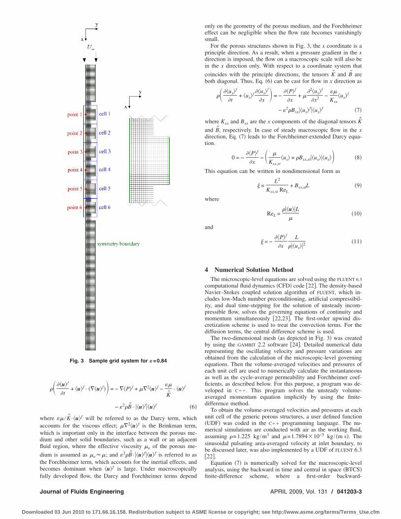
�� u� f

�t+ �u� f · ��u� f� = − ��P� f + ��2�u� f −

��

K�· �u� f

− �2�B� · �u� f�u� f �6�

where �� /K� · �u� f will be referred to as the Darcy term, whichaccounts for the viscous effect; ��2�u� f is the Brinkman term,which is important only in the interface between the porous me-dium and other solid boundaries, such as a wall or an adjacentfluid region, where the effective viscosity �e of the porous me-

dium is assumed as �e��; and �2�B� · �u� f�u� f is referred to asthe Forchheimer term, which accounts for the inertial effects, andbecomes dominant when �u� f is large. Under macroscopicallyfully developed flow, the Darcy and Forchheimer terms depend

only on the geometry of the porous medium, and the Forchheimereffect can be negligible when the flow rate becomes vanishinglysmall.

For the porous structures shown in Fig. 3, the x coordinate is aprinciple direction. As a result, when a pressure gradient in the xdirection is imposed, the flow on a macroscopic scale will also bein the x direction only. With respect to a coordinate system that

coincides with the principle directions, the tensors K� and B� areboth diagonal. Thus, Eq. �6� can be cast for flow in x direction as

�� ux� f

�t+ �ux� f ��ux� f

�x = −

��P� f

�x+ �

�2�ux� f

�x2 −��

Kxx�ux� f

− �2�Bxx�ux� f�ux� f �7�

where Kxx and Bxx are the x components of the diagonal tensors K�

and B� , respectively. In case of steady macroscopic flow in the xdirection, Eq. �7� leads to the Forchheimer-extended Darcy equa-tion.

0 = −��P� f

�x− � �

Kxx,st�ux� + �Bxx,st�ux��ux� �8�

This equation can be written in nondimensional form as

� =L2

Kxx,st ReL+ Bxx,stL �9�

where

ReL =��u�L

��10�

and

� = −��P� f

�x

L

��ux�2�11�

4 Numerical Solution MethodThe microscopic-level equations are solved using the FLUENT 6.3

computational fluid dynamics �CFD� code �22�. The density-basedNavier–Stokes coupled solution algorithm of FLUENT, which in-cludes low-Mach number preconditioning, artificial compressibil-ity, and dual time-stepping for the solution of unsteady incom-pressible flow, solves the governing equations of continuity andmomentum simultaneously �22,23�. The first-order upwind dis-cretization scheme is used to treat the convection terms. For thediffusion terms, the central difference scheme is used.

The two-dimensional mesh �as depicted in Fig. 3� was createdby using the GAMBIT 2.2 software �24�. Detailed numerical datarepresenting the oscillating velocity and pressure variations areobtained from the calculation of the microscopic-level governingequations. Then the volume-averaged velocities and pressures ofeach unit cell are used to numerically calculate the instantaneousas well as the cycle-average permeability and Forchheimer coef-ficients, as described below. For this purpose, a program was de-veloped in C��. This program solves the unsteady volume-averaged momentum equation implicitly by using the finite-difference method.

To obtain the volume-averaged velocities and pressures at eachunit cell of the generic porous structures, a user defined function�UDF� was coded in the C�� programming language. The nu-merical simulations are conducted with air as the working fluid,assuming �=1.225 kg /m3 and �=1.7894�10−5 kg / �m s�. Thesinusoidal pulsating area-averaged velocity at inlet boundary, tobe discussed later, was also implemented by a UDF of FLUENT 6.3�22�.

Equation �7� is numerically solved for the macroscopic-levelanalysis, using the backward in time and central in space �BTCS�finite-difference scheme, where a first-order backward-

Fig. 3 Sample grid system for ε=0.84



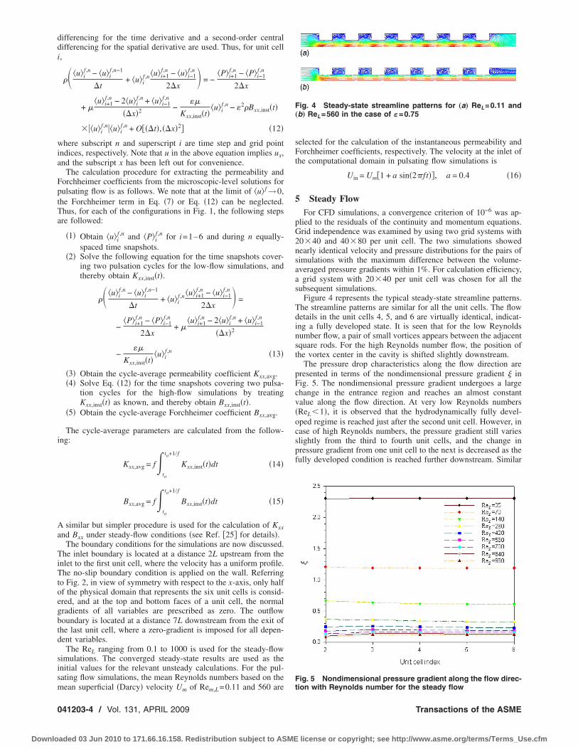
differencing for the time derivative and a second-order centraldifferencing for the spatial derivative are used. Thus, for unit celli,

�� u�if ,n − �u�i

f ,n−1

�t+ �u�i

f ,n �u�i+1f ,n − �u�i−1

f ,n

2�x = −

�P�i+1f ,n − �P�i−1

f ,n

2�x

+ ��u�i+1

f ,n − 2�u�if ,n + �u�i−1

f ,n

��x�2 −��

Kxx,inst�t��u�i

f ,n − �2�Bxx,inst�t�

��u�if ,n�u�i

f ,n + O��t�,��x�2� �12�

where subscript n and superscript i are time step and grid pointindices, respectively. Note that u in the above equation implies ux,and the subscript x has been left out for convenience.

The calculation procedure for extracting the permeability andForchheimer coefficients from the microscopic-level solutions forpulsating flow is as follows. We note that at the limit of �u� f →0,the Forchheimer term in Eq. �7� or Eq. �12� can be neglected.Thus, for each of the configurations in Fig. 1, the following stepsare followed:

�1� Obtain �u�if ,n and �P�i

f ,n for i=1–6 and during n equally-spaced time snapshots.

�2� Solve the following equation for the time snapshots cover-ing two pulsation cycles for the low-flow simulations, andthereby obtain Kxx,inst�t�.

�� u�if ,n − �u�i

f ,n−1

�t+ �u�i

f ,n �u�i+1f ,n − �u�i−1

f ,n

2�x =

−�P�i+1

f ,n − �P�i−1f ,n

2�x+ �

�u�i+1f ,n − 2�u�i

f ,n + �u�i−1f ,n

��x�2

−��

Kxx,inst�t��u�i

f ,n �13�

�3� Obtain the cycle-average permeability coefficient Kxx,avg.�4� Solve Eq. �12� for the time snapshots covering two pulsa-

tion cycles for the high-flow simulations by treatingKxx,inst�t� as known, and thereby obtain Bxx,inst�t�.

�5� Obtain the cycle-average Forchheimer coefficient Bxx,avg.

The cycle-average parameters are calculated from the follow-ing:

Kxx,avg = f�to

to+1/f

Kxx,inst�t�dt �14�

Bxx,avg = f�to

to+1/f

Bxx,inst�t�dt �15�

A similar but simpler procedure is used for the calculation of Kxxand Bxx under steady-flow conditions �see Ref. �25� for details�.

The boundary conditions for the simulations are now discussed.The inlet boundary is located at a distance 2L upstream from theinlet to the first unit cell, where the velocity has a uniform profile.The no-slip boundary condition is applied on the wall. Referringto Fig. 2, in view of symmetry with respect to the x-axis, only halfof the physical domain that represents the six unit cells is consid-ered, and at the top and bottom faces of a unit cell, the normalgradients of all variables are prescribed as zero. The outflowboundary is located at a distance 7L downstream from the exit ofthe last unit cell, where a zero-gradient is imposed for all depen-dent variables.

The ReL ranging from 0.1 to 1000 is used for the steady-flowsimulations. The converged steady-state results are used as theinitial values for the relevant unsteady calculations. For the pul-sating flow simulations, the mean Reynolds numbers based on themean superficial �Darcy� velocity Um of Rem,L=0.11 and 560 are

selected for the calculation of the instantaneous permeability andForchheimer coefficients, respectively. The velocity at the inlet ofthe computational domain in pulsating flow simulations is

Uin = Um�1 + a sin�2ft��, a = 0.4 �16�

5 Steady FlowFor CFD simulations, a convergence criterion of 10−6 was ap-

plied to the residuals of the continuity and momentum equations.Grid independence was examined by using two grid systems with20�40 and 40�80 per unit cell. The two simulations showednearly identical velocity and pressure distributions for the pairs ofsimulations with the maximum difference between the volume-averaged pressure gradients within 1%. For calculation efficiency,a grid system with 20�40 per unit cell was chosen for all thesubsequent simulations.

Figure 4 represents the typical steady-state streamline patterns.The streamline patterns are similar for all the unit cells. The flowdetails in the unit cells 4, 5, and 6 are virtually identical, indicat-ing a fully developed state. It is seen that for the low Reynoldsnumber flow, a pair of small vortices appears between the adjacentsquare rods. For the high Reynolds number flow, the position ofthe vortex center in the cavity is shifted slightly downstream.

The pressure drop characteristics along the flow direction arepresented in terms of the nondimensional pressure gradient � inFig. 5. The nondimensional pressure gradient undergoes a largechange in the entrance region and reaches an almost constantvalue along the flow direction. At very low Reynolds numbers�ReL1�, it is observed that the hydrodynamically fully devel-oped regime is reached just after the second unit cell. However, incase of high Reynolds numbers, the pressure gradient still variesslightly from the third to fourth unit cells, and the change inpressure gradient from one unit cell to the next is decreased as thefully developed condition is reached further downstream. Similar

Fig. 4 Steady-state streamline patterns for „a… ReL=0.11 and„b… ReL=560 in the case of ε=0.75

Fig. 5 Nondimensional pressure gradient along the flow direc-tion with Reynolds number for the steady flow



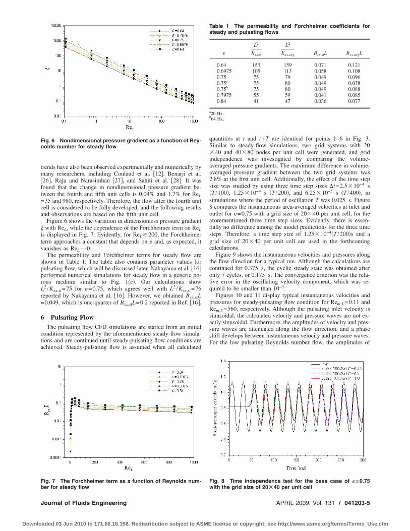
trends have also been observed experimentally and numerically bymany researchers, including Coulaud et al. �12�, Benarji et al.�26�, Raju and Narasimhan �27�, and Sahiti et al. �28�. It wasfound that the change in nondimensional pressure gradient be-tween the fourth and fifth unit cells is 0.04% and 1.7% for ReL=35 and 980, respectively. Therefore, the flow after the fourth unitcell is considered to be fully developed, and the following resultsand observations are based on the fifth unit cell.

Figure 6 shows the variation in dimensionless pressure gradient� with ReL, while the dependence of the Forchheimer term on ReLis displayed in Fig. 7. Evidently, for ReL�200, the Forchheimerterm approaches a constant that depends on � and, as expected, itvanishes as ReL→0.

The permeability and Forchheimer terms for steady flow areshown in Table 1. The table also contains parameter values forpulsating flow, which will be discussed later. Nakayama et al. �16�performed numerical simulations for steady flow in a generic po-rous medium similar to Fig. 1�c�. Our calculations showL2 /Kxx,st=75 for �=0.75, which agrees well with L2 /Kxx,st=76reported by Nakayama et al. �16�. However, we obtained Bxx,stL=0.049, which is one-quarter of Bxx,stL=0.2 reported in Ref. �16�.

6 Pulsating FlowThe pulsating flow CFD simulations are started from an initial

condition represented by the aforementioned steady-flow simula-tions and are continued until steady-pulsating flow conditions areachieved. Steady-pulsating flow is assumed when all calculated

quantities at t and t+T are identical for points 1–6 in Fig. 3.Similar to steady-flow simulations, two grid systems with 20�40 and 40�80 nodes per unit cell were generated, and gridindependence was investigated by comparing the volume-averaged pressure gradients. The maximum difference in volume-averaged pressure gradient between the two grid systems was2.8% at the first unit cell. Additionally, the effect of the time stepsize was studied by using three time step sizes �t=2.5�10−4 s�T /100�, 1.25�10−4 s �T /200�, and 6.25�10−5 s �T /400�, insimulations where the period of oscillation T was 0.025 s. Figure8 compares the instantaneous area-averaged velocities at inlet andoutlet for �=0.75 with a grid size of 20�40 per unit cell, for theaforementioned three time step sizes. Evidently, there is essen-tially no difference among the model predictions for the three timesteps. Therefore, a time step size of 1.25�10−4�T /200�s and agrid size of 20�40 per unit cell are used in the forthcomingcalculations.

Figure 9 shows the instantaneous velocities and pressures alongthe flow direction for a typical run. Although the calculations arecontinued for 0.375 s, the cyclic steady state was obtained afteronly 7 cycles, or 0.175 s. The convergence criterion was the rela-tive error in the oscillating velocity component, which was re-quired to be smaller than 10−3.

Figures 10 and 11 display typical instantaneous velocities andpressures for steady-pulsating flow condition for Rem,L=0.11 andRem,L=560, respectively. Although the pulsating inlet velocity issinusoidal, the calculated velocity and pressure waves are not ex-actly sinusoidal. Furthermore, the amplitudes of velocity and pres-sure waves are attenuated along the flow direction, and a phaseshift develops between instantaneous velocity and pressure waves.For the low pulsating Reynolds number flow, the amplitudes of

Fig. 6 Nondimensional pressure gradient as a function of Rey-nolds number for steady flow

Fig. 7 The Forchheimer term as a function of Reynolds num-ber for steady flow

Table 1 The permeability and Forchheimer coefficients forsteady and pulsating flows

�

L2

Kxx,st

L2

Kxx,avg Bxx,stL Bxx,avgL

0.64 153 159 0.071 0.1210.6975 105 113 0.058 0.1080.75 75 79 0.049 0.0960.75a 75 80 0.049 0.0780.75b 75 80 0.049 0.0880.7975 55 59 0.041 0.0850.84 41 47 0.036 0.077

a20 Hz.b64 Hz,

Fig. 8 Time independence test for the base case of ε=0.75with the grid size of 20Ã40 per unit cell



instantaneous pressure waves along the flow direction decreasenotably; whereas for high Rem,L cases, the reduction in instanta-neous pressure amplitudes is insignificant along the flow direc-

tion, and the waves are flattened with decreasing porosity. Theresults also show that the cycle-average instantaneous velocities atthe measured points increase as the porosity decreases, and as the

Fig. 9 Convergence check for ε=0.75 with 20Ã40 nodes per unit cell for„a… velocity and „b… pressure

Fig. 10 Variation in the instantaneous „a… velocity and „b…pressure waves along the flow direction for Rem,L=0.11 and ε=0.7975

Fig. 11 Variation in the instantaneous „a… velocity and „b…pressure waves along the flow direction for Rem,L=560 and ε=0.84



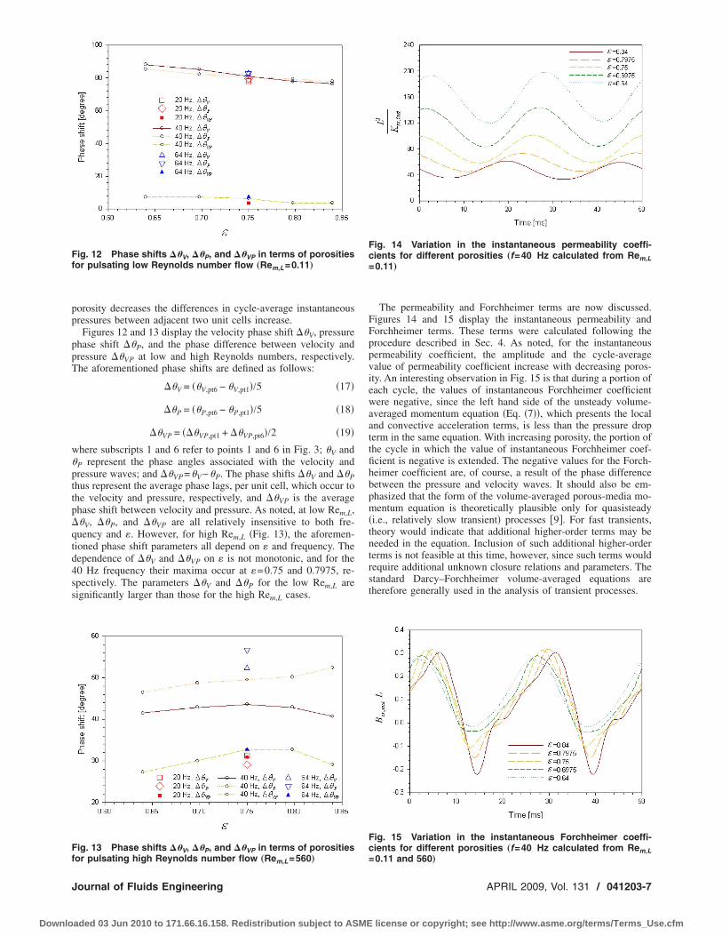
porosity decreases the differences in cycle-average instantaneouspressures between adjacent two unit cells increase.

Figures 12 and 13 display the velocity phase shift ��V, pressurephase shift ��P, and the phase difference between velocity andpressure ��VP at low and high Reynolds numbers, respectively.The aforementioned phase shifts are defined as follows:

��V = ��V,pt6 − �V,pt1�/5 �17�

��P = ��P,pt6 − �P,pt1�/5 �18�

��VP = ��VP,pt1 + ��VP,pt6�/2 �19�

where subscripts 1 and 6 refer to points 1 and 6 in Fig. 3; �V and�P represent the phase angles associated with the velocity andpressure waves; and ��VP=�V−�P. The phase shifts ��V and ��Pthus represent the average phase lags, per unit cell, which occur tothe velocity and pressure, respectively, and ��VP is the averagephase shift between velocity and pressure. As noted, at low Rem,L,��V, ��P, and ��VP are all relatively insensitive to both fre-quency and �. However, for high Rem,L �Fig. 13�, the aforemen-tioned phase shift parameters all depend on � and frequency. Thedependence of ��V and ��VP on � is not monotonic, and for the40 Hz frequency their maxima occur at �=0.75 and 0.7975, re-spectively. The parameters ��V and ��P for the low Rem,L aresignificantly larger than those for the high Rem,L cases.

The permeability and Forchheimer terms are now discussed.Figures 14 and 15 display the instantaneous permeability andForchheimer terms. These terms were calculated following theprocedure described in Sec. 4. As noted, for the instantaneouspermeability coefficient, the amplitude and the cycle-averagevalue of permeability coefficient increase with decreasing poros-ity. An interesting observation in Fig. 15 is that during a portion ofeach cycle, the values of instantaneous Forchheimer coefficientwere negative, since the left hand side of the unsteady volume-averaged momentum equation �Eq. �7��, which presents the localand convective acceleration terms, is less than the pressure dropterm in the same equation. With increasing porosity, the portion ofthe cycle in which the value of instantaneous Forchheimer coef-ficient is negative is extended. The negative values for the Forch-heimer coefficient are, of course, a result of the phase differencebetween the pressure and velocity waves. It should also be em-phasized that the form of the volume-averaged porous-media mo-mentum equation is theoretically plausible only for quasisteady�i.e., relatively slow transient� processes �9�. For fast transients,theory would indicate that additional higher-order terms may beneeded in the equation. Inclusion of such additional higher-orderterms is not feasible at this time, however, since such terms wouldrequire additional unknown closure relations and parameters. Thestandard Darcy–Forchheimer volume-averaged equations aretherefore generally used in the analysis of transient processes.

Fig. 12 Phase shifts ��V, ��P, and ��VP in terms of porositiesfor pulsating low Reynolds number flow „Rem,L=0.11…

Fig. 13 Phase shifts ��V, ��P, and ��VP in terms of porositiesfor pulsating high Reynolds number flow „Rem,L=560…

Fig. 14 Variation in the instantaneous permeability coeffi-cients for different porosities „f=40 Hz calculated from Rem,L=0.11…

Fig. 15 Variation in the instantaneous Forchheimer coeffi-cients for different porosities „f=40 Hz calculated from Rem,L=0.11 and 560…



The cycle-average permeability and Forchheimer terms areshown in Figs. 16 and 17, respectively, and their numerical valuesare provided in Table 1. In both figures, model predictions areshown for f =40 Hz for all porosities of interest. For �=0.75,however, model predictions for f =20 Hz and 60 Hz are also de-picted. Furthermore, in both figures the parameters representingsteady-flow conditions are also shown for comparison. The per-meability parameter, as noted in Fig. 16, is a strong function ofporosity and monotonically decreases as porosity is increased.More importantly, furthermore, the cycle-average permeability pa-rameter for pulsating flow is only slightly larger than the perme-ability parameter for steady flow �or, equivalently, the permeabil-ity for pulsating flow is only slightly larger than the permeabilityfor steady flow�. On the other hand, as noted in Fig. 17, the cycle-average Forchheimer coefficients decrease with increasing poros-ity and are about two times larger than those for steady flow at thesame porosity. It is also noted in Fig. 17 that the Forchheimerparameter depends on the frequency, and its dependence on fre-quency is not monotonic. Our simulation results, although rela-tively limited in scope and parametric range, thus suggest that theapplication of the Darcy–Forchheimer model equations withsteady-flow parameters to pulsating flow is, in general, incorrect.While the permeability is likely to be approximately the same forsteady and pulsating flow conditions, the Forchheimer coefficientcan have significantly different values for steady-flow and pulsat-ing flow conditions. More comprehensive investigations are rec-ommended for better understanding the trends and dependenciesin pulsating flow.

7 ConclusionsWe have investigated, by numerical simulation, the momentum

transfer parameters associated with pulsating laminar flowthrough generic porous media made of periodic square cylinderspatterned on a rectangular pitch, for flow pulsation frequencies of20–64 Hz and the porosity ranging from 0.64–0.84. Detailed nu-merical data representing the oscillating two-dimensional velocityand pressure variations were obtained by solving the Navier–Stokes using the CFD code FLUENT 6.3. These numerical datawere then utilized for the calculation of various volume-averagedproperties to be used in the standard Darcy-extended Forchheimermomentum equation. Instantaneous and cycle-average parameterswere both extracted and displayed. The results indicated that theapplication of the Darcy-extended Forchheimer momentum equa-tion with coefficients representing steady flow to pulsating flowconditions is only adequate at very low-flow �low frequency� con-ditions and is otherwise incorrect. Within the range of parametersstudied in this investigation, the pulsating flow cycle-average per-meabilities were a strong function of porosity, but they were onlyslightly larger than the permeabilities for steady flows. The cycle-average Forchheimer coefficients for pulsating flows strongly de-pended on frequency, however, and were significantly larger thansteady-flow Forchheimer coefficients.

The results also showed that the velocity and pressure phaseshifts are sensitive to the mean-flow Reynolds number. The veloc-ity phase shifts ��V and pressure phase shifts ��P for low mean-flow Reynolds numbers �Rem,L=0.11� were significantly largerthan those for the high-flow Reynolds number �Rem,L=560� flows.However, the phase shifts between velocity and pressure ��VP forRem,L=560 were several times larger than those for the Rem,L=0.11 case.

Nomenclaturea normalized amplitude of velocityA constantB Forchheimer coefficient �1/m�

Bxx,avg cycle-average Forchheimer coefficient �m2�Bxx,inst instantaneous Forchheimer coefficient along

the x direction for pulsating flow �m2�Bxx,st Forchheimer coefficient along the x direction

for steady flow �m2�B� Forchheimer coefficient tensor �1/m�D side of square rod �m�f frequency �Hz�I identity tensor

K permeability coefficient �m2�Kxx,avg cycle-average permeability coefficient �m2�Kxx,inst instantaneous permeability coefficient along the

x direction for pulsating flow �m2�Kxx,st permeability coefficient along the x direction

for steady flow �m2�K� permeability tensor �m2�L length of unit cell �m�P static pressure �N /m2�

�P� f intrinsic volume-average fluid static pressureover Vf �N /m2�

ReL Reynolds number based on a unit cell length Lin steady flow

Rem,l Reynolds number based on mean velocity andunit cell length �pulsating flow�

t time �s�T period of pulsation �s�

u, U velocity �m/s��u� superficial volume-average fluid velocity �m/s�

�u� f intrinsic volume-average fluid velocity �m/s�V averaging control volume �m3�

Fig. 16 Comparison of the permeability coefficients betweenthe steady and pulsating flow for different porosities

Fig. 17 Comparison of the Forchheimer coefficients betweenthe steady and pulsating flow for different porosities



Vf fluid volume in an averaging control volume�m3�

�t time step size �s�

Greek Letters� porosity of medium� molecular viscosity �kg /m s�� kinematic viscosity �m2 /s�� phase angle �deg�� density �kg /m3�

��V phase shift of velocity �deg��P phase shift of pressure �deg�

��VP phase shift between velocity and pressure �deg�� nondimensional pressure gradient

Subscriptsavg cycle-average value

e effectiveexit exit

i grid point indexin inlet

inst instantaneous valuem mean valuest steady state

x, xx x direction

Superscriptsf fluidn time step index= tensor

References�1� Ju, Y. L., Wang, C., and Zhou, Y., 1998, “Numerical Simulation and Experi-

mental Verification of the Oscillating Flow in Pulse Tube Refrigerator,” Cryo-genics, 38, pp. 169–176.

�2� Hsu, C. T., Fu, H. L., and Cheng, P., 1999, “On Pressure Velocity Correlationof Steady and Oscillating Flows in Regenerators Made of Wire-Screens,”ASME J. Fluids Eng., 121, pp. 52–56.

�3� Nam, K., and Jeong, S., 2002, “Experimental Study on the Regenerator UnderActual Operating Conditions,” Adv. Cryog. Eng., 47, pp. 977–984.

�4� Jeong, S., Nam, K., and Jung, J., 2002, “Regenerator Characterization UnderOscillating Flow and Pulsating Pressure,” Cryocoolers, 12, pp. 531–537.

�5� Cha, J. S., Ghiaaisiaan, S. M., Desai, P. V., Harvey, J. P., and Kirkconnell, C.S., 2006, “Multi-Dimensional Flow Effects in Pulse Tube Refrigerators,”Cryogenics, 46, pp. 658–665.

�6� Clearman, W. M., Cha, J. S., Ghiaasiaan, S. M., and Kirkconnell, C. S., 2008,“Anisotropic Steady-Flow Hydrodynamic Parameters of Microporous MediaApplied to Pulse Tube and Stirling Cryocooler Regenerator,” Cryogenics, 48,pp. 112–121.

�7� Whitaker, S., 1973, “The Transport Equations for Multi-Phase Systems,”

Chem. Eng. Sci., 28, pp. 139–147.�8� Gray, W. G., and O’Neill, K., 1976, “On the General Equation for Flow in

Porous Media and Their Reduction to Darcy’s Law,” Water Resour. Res., 12,pp. 148–154.

�9� Kaviany, M., 1995, Principles of Heat Transfer in Porous Media, 2nd ed.,Springer-Verlag, Berlin.

�10� Quintard, M., Kaviany, M., and Whitaker, S., 1997, “Two-Medium Treatmentof Heat Transfer in Porous Media: Numerical Results for Effective Properties,”Adv. Water Resour., 20, pp. 77–94.

�11� Moyne, C., Didierjean, S., Amaral Souto, H. P., and da Silveira, O. T., 2000,“Thermal Dispersion in Porous Media: One Equation Model,” Int. J. HeatMass Transfer, 43, pp. 3853–3867.

�12� Coulaud, O., Morel, P., and Caltagiorne, J. P., 1988, “Numerical Modeling ofNonlinear Effects in Laminar Flow Through a Porous Medium,” J. FluidMech., 190, pp. 393–407.

�13� Kuwahara, F., Nakayama, A., and Koyama, H., 1996, “A Numerical Study ofThermal Dispersion in Porous Media,” ASME J. Heat Transfer, 118, pp. 756–761.

�14� Kuwahara, F., Shirota, M., and Nakayama, A., 2001, “A Numerical Study ofInterfacial Convective Heat Transfer Coefficient in Two-Energy EquationModel for Convection in Porous Media,” Int. J. Heat Mass Transfer, 44, pp.1153–1159.

�15� Kuwahara, F., Yamane, T., and Nakayama, A., 2006, “Large Eddy Simulationof Turbulent Flow in Porous Media,” Int. Commun. Heat Mass Transfer, 33,pp. 411–418.

�16� Nakayama, A., Kuwahara, F., Umemoto, T., and Hayashi, T., 2002, “Heat andFluid Flow Within an Anisotropic Porous Medium,” ASME J. Heat Transfer,124�4�, pp. 746–753.

�17� Nakayama, A., Kuwahara, F., and Kodama, Y., 2006, “An Equation for Ther-mal Dispersion Flux Transport and Its Mathematical Modeling for Heat Trans-fer and Fluid Flow in a Porous Medium,” J. Fluid Mech., 563, pp. 81–96.

�18� Nakayama, A., Kuwahara, F., and Sano, Y., 2007, “Concept of EquivalentDiameter for Heat and Fluid Flow in Porous Media,” AIChE J., 53, pp. 732–736.

�19� Vafai, K., and Tien, C. L., 1981, “Boundary and Inertia Effects on Flow andHeat Transfer in Porous Media,” Int. J. Heat Mass Transfer, 24, pp. 195–203.

�20� Vafai, K., and Amiri, A., 1998, “Non-Darcian Effects in Confined ForcedConvective Flows,” Transport Phenomena in Porous Media, D. B. Ingham andI. Pope, eds., Pergamon, New York.

�21� Hsu, C. T., and Cheng, P., 1990, “Thermal Dispersion in a Porous Medium,”Int. J. Heat Mass Transfer, 33, pp. 1587–1597.

�22� FLUENT Inc., 2006, “Fluent 6 User Manual.�23� Weiss, J. M., and Smith, W. A., 1995, “Preconditioning Applied to Variable

and Constant Density Flows,” AIAA J., 33, pp. 2050–2057.�24� FLUENT Inc., 2006, “GAMBIT 2 User Manual.�25� Kim, S.-M., 2008, “Numerical Investigation on Laminar Pulsating Flow

Through Porous Media,” MS thesis, Georgia Institute of Technology, Atlanta,GA.

�26� Benarji, N., Balaji, C., and Venkateshan, S. P., 2008, “Unsteady Fluid Flowand Heat Transfer Over a Bank of Flat Tubes,” Heat Mass Transfer, 44, pp.445–461.

�27� Raju, K. S., and Narasimhan, A., 2007, “Porous Medium Interconnector Ef-fects on the Thermohydraulics of Near-Compact Heat Exchangers Treated asPorous Media,” ASME J. Heat Transfer, 129, pp. 273–281.

�28� Sahiti, N., Lemouedda, A., Stojkovic, D., Durst, F., and Franz, E., 2006, “Per-formance Comparison of Pin Fin In-Duct Flow Arrays With Various Pin Cross-Sections,” Appl. Therm. Eng., 26, pp. 1176–1192.



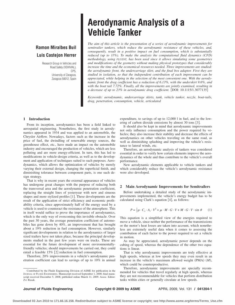
Ramon Miralbes Buil

Luis Castejon Herrer

Research Group in Vehicles andRoad Safety (VEHIVIAL),

CPS,University of Zaragoza,Zaragoza 50012, Spain

Aerodynamic Analysis of aVehicle TankerThe aim of this article is the presentation of a series of aerodynamic improvements forsemitrailer tankers, which reduce the aerodynamic resistance of these vehicles, and,consequently, result in a positive impact on fuel consumption, which is substantiallyreduced (up to 11%). To make the analysis the computational fluid dynamics (CFD)methodology, using FLUENT, has been used since it allows simulating some geometriesand modifications of the geometry without making physical prototypes that considerablyincrease the time and the economical resources needed. Three improvements are studied:the aerodynamic front, the undercarriage skirt, and the final box adaptor. First they arestudied in isolation, so that the independent contribution of each improvement can beappreciated, while helping in the selection of the most convenient one. With the aerody-namic front the drag coefficient has a reduction of 6.13%, with the underskirt 9.6%, andwith the boat tail 7.72%. Finally, all the improvements are jointly examined, resulting ina decrease of up to 23% in aerodynamic drag coefficient. �DOI: 10.1115/1.3077135�

Keywords: aerodynamic, undercarriage skirts, tank, vehicle tanker, nozzle, boat-tails,drag, penetration, consumption, vehicle, articulated

1 IntroductionFrom its inception, aerodynamics has been a field linked to

aerospatial engineering. Nonetheless, the first study in aerody-namics appeared in 1934 and was applied to an automobile, theChrysler Airflow. Nowadays, factors such as the increase in theprice of fuel, the dwindling of renewable energy sources, thegreenhouse effect, etc., have made an impact on the automobileindustry and encouraged the production of vehicles, which are lesspolluting and are more energy-efficient. In turn, this has led tomodifications in vehicle-design criteria, as well as to the develop-ment and application of techniques suited to such purposes. Aero-dynamics, which allows the optimization of vehicles by merelyvarying their external design, changing the superficial finish, anddiminishing tolerance between component parts, is one such de-sign strategy.

That is why in recent years the external appearance of vehicleshas undergone great changes with the purpose of reducing boththe transversal area and the aerodynamic penetration coefficient,replacing the straight lines of yesteryear with new and sinuousshapes and more stylized profiles �1�. These developments are theresult of the application of strict efficiency and economic profit-ability criteria, since approximately half of the energy used by avehicle is used to counteract the resistance of the atmosphere. Thisin itself would suffice to prove the importance of aerodynamics,which is the only way of overcoming this invisible obstacle. Overthe past 30 years, the average penetration coefficient of automo-biles has gone down by 40%, an improvement that has broughtabout a 19% reduction in fuel consumption. However, similarlysignificant developments in relation to the aerodynamics of largersized trailers have not taken place, because the principal develop-ments studied in the past few years were on trucks. These areessential for the future development of more environmentally-friendly vehicles; should improvements be carried out, they couldentail a feasible 15% �2� reduction in fuel consumption.

Therefore, 20% improvements in a vehicle’s aerodynamic pen-etration coefficient can lead to savings of up to 10% in annual

expenditure, to savings of up to 12,000 l in fuel, and to the low-ering of carbon dioxide emissions by almost 30 tons �3�.

It should also be kept in mind that aerodynamic improvementsnot only influence consumption and the power required by ve-hicles; they also increase their stability and decrease the effects ofaerodynamics on other vehicles traveling on the same road, aswell as diminishing splashing and improving the vehicle’s resis-tance to lateral winds, etc.

Therefore, an aerodynamic analysis of tankers was consideredessential in order to verify how certain elements improve the aero-dynamics of the whole and thus contribute to the vehicle’s overallperformance.

New aerodynamic elements applicable to vehicle tankers andwhich considerably reduce the vehicle’s aerodynamic resistancewere also developed.

2 Main Aerodynamic Improvements for SemitrailersBefore undertaking a detailed study of the aerodynamic im-

provements implemented, the vehicle’s energy budget has to becalculated using Clark’s equation �4�, as follows:

P = 12� · Cx · At · V3 + � · M · G · V + M · G · V · sin � �1�

This equation is a simplified view of the energies required tomove a vehicle, since neither the performance of the transmissionsor the motor’s heat losses are taken into account, which nonethe-less are extremely useful data when it comes to assessing thecontribution of each factor to the power required to set a vehiclein motion.

As may be appreciated, aerodynamic power depends on thecubing of speed, whereas the dependence of the other two equa-tions is linear.

That is why aerodynamic improvements are truly effective athigh speeds, whereas at low speeds they may even result in anincrease in the vehicle’s maximum allowed weight �PMA� �M�,which could be counterproductive.

Therefore, aerodynamic improvements are specially recom-mended for vehicles that travel regularly at high speeds, whereasthey are not recommendable for vehicles that perform distributiontasks within cities or generally circulate at low speeds.

Contributed by the Fluids Engineering Division of ASME for publication in theJOURNAL OF FLUIDS ENGINEERING. Manuscript received September 1, 2008; final manu-script received December 5, 2008; published online March 11, 2009. Assoc. Editor:Zvi Rusak.



If we look closely at the previous equation we see that the mainfactors that can be modified are the vehicle’s transversal area �At�,the aerodynamic coefficient �Cx�, and the tire friction coefficient�� with low consumption tires.

Regarding the vehicle’s transversal area, we may notice that thewidth of an articulated vehicle designed for the transport of com-modities is determined both by the width of the tractor and by itsheight. However, the use of tankers with a low level chassis di-minishes the overall height and allows the use of tractors with alower height or smaller superior spoilers.

As far as the aerodynamic resistance coefficient is concerned,several aerodynamic improvements will lower this coefficient.Among these, a distinction must be made between those whichapply to the tractor and those which apply to the semitrailer,which is responsible for up to 70% of aerodynamic losses �seeFig. 1�. These losses could be reduced by up to 40% by using theavailable technology and would equate to a 28% reduction in theaerodynamic resistance coefficient. Figure 1 shows the high pres-sure areas of an articulated vehicle associated with high aerody-namic losses.

If we manage to lower the effects of pressure on each of theseareas, the overall aerodynamics of the vehicle will therefore im-prove considerably.

It should be pointed out that latter-day aerodynamic improve-ments are applied mainly to square box �5� vehicles and thereforehave to be adapted for their use with tankers. Among these, wewill be examining boat-tails, aerodynamic undercarriage skirtsand aerodynamic fairings.

2.1 Boat-Tails . Boat-tails �see Fig. 2� prevent the detachmentof the outer layer of the rear end of the box by preventing pressuregradients that would generate vorticity.

There are several possible boat-tail configurations. One is theuse of rear plates �up to 4% aerodynamic improvement�. Anotheris the application of round beam sections �up to 5%� �6� to the rear

area of the box, although the use of one type of boat-tail or theother depends on the type of box, the maximum size of the ve-hicle, etc.

2.2 Aerodynamic Fairings. These aerodynamic elements arefixed on the upper front area of the semitrailer �see Fig. 3� andredirect the air flow that appears in that area toward the box,keeping it out of the king-pin cavity and thus involving an aero-dynamic improvement of up to 3% �7�.

2.3 Aerodynamic Undercarriage Skirt. This part preventsthe entry of air in the lower part of the vehicle, both in the tractorarea and the semitrailer area, decreasing air flow in these areas,which due to the wheels and several parts of the vehicle’s lowerarea would otherwise generate a turbulent flow that would ad-versely affect the vehicle’s aerodynamics. A decrease of up to 7%�8� can be achieved this way �see Fig. 4�.

3 Methodology for Aerodynamic Calculation UsingCFD

A commercial aerodynamic program was used for the aerody-namic calculation of the vehicle and its possible modifications.The following methodology was used for modeling, discretiza-tion, and vehicle calculation.

3.1 Computer Aided Design (CAD) Modeling. In order toproceed with the analysis, the first step is to perform CAD mod-eling of the vehicle’s outer area and remove or simplify certainelements, such as the vehicle’s rearview mirrors, turn signals,small external accessories, sleeves, and other auxiliary elements,as the modeling of these elements would involve an excessivelycomplex and detailed finite element model �9,10�.

In our particular case, a CAD model faithfully reflecting theexternal dimensions of both the vehicle and the tractor was de-signed, and therefore we chose to use the main dimensions of atanker supplied by CryoEnergy S. A. �Tarrega, Spain� �11�, towhich a medium range tractor was added �see Figs. 5 and 6�.

This cab was used as a basis, removing all the optional aerody-

Fig. 1 Wind-averaged drag values for an articulated vehiclewith a square box †4‡

Fig. 2 Boat-tails

Fig. 3 Aerodynamic fairings



namic accessories that may come with it: spoiler, lateral air flowstreamliners, and bumper spoiler. These elements were not used,as we only intended to affect the semitrailer. The reason for notusing them is that since these elements are cab accessories, not all

cabs employ them, and also that, due to the fact that they havebeen studied and optimized in depth, these elements have manydifferent configurations and shapes.

The air inlet of the vehicle’s radiator was also left out of themodeling, because taking this factor into account would have re-quired a very elaborate model of the vehicle, which would, inturn, have involved numerical complications that would havemade calculation unfeasible. Besides, the contribution of this partto the global model is relatively small and is not under study here�9,10,12�.

As far as the tanker is concerned, the turn signals, sleeves, andtubes of the lower area of the tanker, etc., were removed.

The several elements, which comprise the tanker’s lower area,were not removed, since this is one of the areas under study,despite the fact that this entails an increase both in the complexityof the model and in the number of elements that comprise it.

In relation to the tire area, the wheel pitch and the empty spaceswithin it, along with its dimensions, were maintained in order tocorrectly model the contribution of these elements to the vehicle,since the tire area significantly affects the vehicle’s overall aero-dynamics and is one of the areas subject to study �9,10,12�. It maybe worth pointing out that a symmetrical model was used to re-duce the necessary computational cost. Consequently, only halfthe vehicle was modeled.

3.2 Discretization Through Volumetric Elements. In orderto perform modeling using volumetric elements, the vehicle’sCAD was taken as the starting point and introduced into a volume,which is to simulate the air on the outside of the vehicle. Thefollowing volume—in keeping with the recommendations of otherauthors �9,10,12� and those of the program—was considered forthis purpose �12�.

In theory, there should be a distance of 2000 mm in the airvolume of a vehicle similar to the one selected between the frontpart of the vehicle and the air inlet, and a distance of 10,000 mmbetween the end of the vehicle and the air outlet in order to per-fectly collect the slipstream generated by the vehicle. Regardingboth lateral and superior distances, these should be at least 4000mm in relation to the outermost tangent surface.

The dimensions of this volume are such that the air circulatingin the areas furthest from the vehicle is not altered by the latter,which implies that the imposition of contour conditions on theouter area of the volume will not be altered by the vehicle, as thiswould involve a modification of the model’s air flows and, conse-quently, an error in the results.

Fig. 4 Aerodynamic undercarriage skirt

Fig. 5 Baseline equipment trailer

Fig. 6 Baseline equipment trailer



The next step was to extract the vehicle’s volume from the totalvolume, with which we could obtain a “negative image” of thevehicle with regards to how discretization will be carried out

To do so, a tetrahedral mesh with lineal Lagrange elements waschosen, because it allows moderately simple vehicle discretizationand an optimum degree of approximation in relation to computa-tional cost.

First of all, discretization of the outer surfaces was performedboth on the inside and on the outside. The size of these surfaceelements depends on the area in which discretization is carried out�9,10,12�, on its magnitude and on previous experience, althoughit was attempted to reduce the number of elements to the mini-mum, with the proviso that they be as equilateral as possible inorder to ensure convergence and reduce time and calculation re-quirements. A more elaborate discretization was performed inthose areas where greater speed gradients were expected, allowingfor improved simulation of air flow in those areas: the wheelpitch, the front of the vehicle, the area between the cab, and thetank and the rear part of the vehicle, where detachment of theouter layer will occur.

After the discretization of the surfaces was performed, “bound-ary layers” �13� were imposed. This procedure allows us to per-

form fine meshing of the zones immediately surrounding the sur-faces of the vehicle in order to faithfully model the vehicle’s outerlayer. To this end, an initial element size of 6 mm and a boundarylayer of three elements with a mesh growth factor of 1.2 �9,10,12�was chosen. The reason for building such a mesh was to try tocorrectly approximate the outer layer, despite the fact that thisentails a substantial increase in the number of elements and anincrease in computational cost; however, this is justifiable and wasnecessary for the correct modeling of the outer layer of fluid.

Following this, discretization of the remaining air volume wascarried out; in order to do so, meshing of the outer area with alarger size element �1000 mm� was performed, since attached flowwill be preponderant in this area and there will be no flow alter-ations or speed gradients. In order to perform discretization, a sizefunction was used, allowing control of the growth size of theelements from the vehicle to the outside area. To achieve this, amaximum element size of 1000 mm and a 1.2 growth factor—themaximum recommended by the program—was imposed. In thisway, discretization with the most equilateral surfaces possible canbe achieved �see Figs. 7 and 8�.

Fig. 7 Mesh of the baseline equipment trailer „rear zone…

Fig. 8 Mesh of the baseline equipment trailer „middle zone and tractor…



3.3 Aerodynamic Calculation. In order to perform aerody-namic calculation, several tasks have to be carried out prior to thecalculation proper:

3.3.1 Definition of Solution Options. A “segregated” solutionmodel—recommended for this type of calculations—was chosenin order to lower computational requirements. This model uses adouble precision calculation �recommended for aerodynamic cal-culation of vehicles� �14,15� for a stationary �steady� model basedon node calculation and is recommended by the program in orderto achieve better results with this type of calculation.

3.3.2 Definition of the Turbulence Model. A turbulence modelbased on k-� type realizable Reynolds average Navier-Stokes�RANS� equations �14–16� and a wall treatment with nonequili-brated flow were chosen �17�. The choice of this turbulence modelwas mainly due to the fact that nowadays it is the most commonlyused one for aerodynamic calculations and because it also offersan optimum degree of approximation in regard to computationalrequirements.

3.3.3 Definition of Contour Conditions. Since there are severalareas, different contour conditions were considered for each ofthem. An air flow at a constant speed �30 m/s� in a tangentialdirection �7� with very low turbulence �0.1% turbulence intensity�was introduced for the entry boundary, which means that any flowthat there may be will be laminar. Regarding the upper, lateral,and rear areas, these were simulated as being open to the outside,with a pressure of 1 atm and an air flow of 30 m/s in the relevantdirection.

The ground was modeled as a smooth surface traveling at thesame speed as the fluid �30 m/s� �18�, and the wheels were con-sidered smooth and rotational surfaces, coherent with the speed ofthe vehicle �17�.

Symmetry was imposed on the interior wall and the vehicle’swalls were considered fixed and smooth walls without friction.This was due to the fact that the contribution of friction betweenthe fluid and the surface in relation to the global model representsless than 10% of the resistant contribution and that the implemen-tation of this contribution would entail a substantial increase incomputational cost and might even have lead to divergent results.Nonetheless, it would be useful to establish, very precisely and bymeans of experiments, the friction coefficient of each of the mod-el’s superficial finish types in order to establish their contributionto the aerodynamic resistance, which would not be substantiallymodified by variations in the vehicle’s geometry, since the latterdepends mainly on the choice of superficial finishes.

Thus, simulation of the movement of the vehicle is possible, butfrom the relative viewpoint of the tanker.

3.3.4 Selection of Options for Solving the Equations. ASIMPLE-C �13� type resolution algorithm was chosen to solve the

pressure-speed fields, which is the appropriate resolution schemefor discretizations with elements not aligned with the flow �19�. Inaddition, standard discretization schemes were used for pressuresolution and second order schemes were used for calculating mo-mentum and turbulence. These are the parameters recommendedby the program for this type of calculations.

It should be pointed out that in order to improve the model’sconvergence, first order equations were used for calculating mo-mentums and turbulences during the first 300 iterations and thatthe second order scheme was implemented subsequently.

4 Adaptation of Aerodynamic Improvements to theTankers

In this paper, only those aerodynamic improvements directlyapplicable to cryogenic tanks will be analyzed; and therefore, de-spite the fact that they improve the aerodynamics of the tank area,the improvements applied to the tractor will not be taken intoaccount in this study.

Before proceeding with the analysis, it should be pointed outthat aerodynamic resistance coefficients for latter-day articulatedvehicles can be extracted from article 20, and that these can beused to verify the results obtained in the calculation of the originalvehicle. Thus, the aerodynamic resistance coefficient of a vehiclewith the characteristics of the one we are dealing with is roughly0.69.

As a starting point for the analysis of this type of vehicles, theway in which air flow covers the outer surface of the vehicle mustbe understood qualitatively. In order to do so, we will set out fromthe previous experience existing regarding automobiles �20–22�.

On the basis of this information it may be presumed that in atanker-type articulated vehicle �23�, there will be a flow of par-ticles like the one shown in Fig. 9. Therefore, just like in a car,there will be an area at the front where particles will stagnate dueto their collision with the frontal area, although since our frontalarea is much larger and its aerodynamic shape is much less styl-ized than a car’s, and also because this area is perpendicular to theflow, this area will be much larger. There will also be an area nearthe king-pin cavity in which the outer boundary will become de-tached due to the existence of the said cavity, whereas the par-ticles entering the cavity will collide with its rear part, creating aturbulent zone and, presumably, low longitudinal speed and highvorticity.

Since the external geometry of the tank has no protuberances,projections, cavities, etc., it is likely that coupling will recur be-hind the cavity of the king-pin, and therefore, that there will beattached flow in this area.

In the vehicle’s rear area, where the surface ends, flow separa-tion will recur, presumably with low longitudinal speed, and aturbulent slipstream will be generated behind the vehicle.

Fig. 9 Flow around a semitrailer tanker „side view…



The existence of turbulent flow in the lower part of the vehiclemay be presumed due to the large amount of elements and pro-jections in that area. Besides, the presence of the wheels and theirturning will generate turbulence and additional flow detachment.

When we speak of null speed we assume a viewpoint relative tothe vehicle.

Once the flow was theoretically established, the next step was anumerical verification of the hypotheses set forth; therefore, nu-merical calculation and postprocessing of the original configura-tion of the articulated vehicle was carried out.

Total forces and aerodynamic coefficients for all configurationsare reflected in Table 1.

The global aerodynamic resistance coefficient is 0.618, which iswithin the established range for this type of vehicles �24�. Thiscoefficient is somewhat high, because a tractor without aerody-namic elements—which involve considerable aerodynamicpenalization—was used. This is also appreciable in relation to thecontribution of each part of the articulated vehicle to the globalresistance coefficient: 55.4% in the tractor and 44.6% in the body.It should also be pointed out that the body’s contribution to thevehicle’s average total drag is inferior to the 65–75% range indi-cated in Fig. 1. This is because this figure established the contri-bution for a square box semitrailer, the aerodynamic coefficient ofwhich is usually 5% superior to that of a semitrailer tanker �18�and due to the use of a vehicle with aerodynamic improvements inthe tractor.

Once the correctness of the aerodynamic resistance coefficientand the resistant forces of the vehicle have been established, thenext step is to analyze the several areas, which make up the ve-hicle so as to verify in which areas flow detachment occurs andturbulent flow predominates. In order to do so, we analyzed pres-sure maps �high pressures indicate vorticity and turbulent flow�,speed maps �low relative speeds indicate vorticity and turbulent

flow�, turbulence energy maps, and particle flow maps �draft lineswere analyzed in order to perform this analysis, as well as ananalysis of the flow of particles in motion, which was not includedhere due to its being a moving image�.

It must be pointed out that in order to keep the article relativelyshort, only the more representative images of the vehicle wereincluded.

As shown in Fig. 10 and predicted earlier, the low speed areasare the lower part of the vehicle, the king-pin cavity area and theslipstream of the tank; i.e., these are the areas with greater turbu-lence and higher pressures. This figure shows the longitudinalspeed of the vehicle. It shows the wake in the rear part of thevehicle and indicates a high aerodynamical resistance. It alsoshows, in the bottom part of the vehicle past the tractor, a zonewith low velocity and the same in the wheel zone of the tanker.This indicates high aerodynamical losses too. Analyzing Figs. 11and 12 that show the k turbulence parameter and then the zoneswith high aerodynamical losses, these match with the zones pre-viously mentioned and with Fig. 9, so these zones should bemodified to improve the aerodynamics. These zones also havewhirls that indicate turbulence �see Fig. 10 and 13� and causeaerodynamical losses, usually because the geometry of the vehicleis discontinuous, and the attached flow changes to a turbulenceone. In Fig. 10 there is a zero velocity zone in the gap between thetractor and the trailer and it matches with a high losses zone �seeFigs. 11 and 15�.

We also notice in Figs. 10 and 13 a stagnation zone in the frontarea �that is one of the zones with high aerodynamical losses ofthe tractors�, the detachment of the outer layer above the cab inthe vehicle’s rear part and the lower part of the tractor, as well as��coupling�� of the flow in the upper part of the tank �all waspredicted in Fig. 9�.

Table 1 Total resistant forces and aerodynamic resistance coefficients of all the cases considered



Moreover, we may appreciate high fluid speeds �which arecompletely normal� on the edges of the tractor �see Figs. 14 and15� as a result of the latter’s stagnation.

If we perform a cut, which is parallel to the plane of symmetryand near the lateral surface of the cab, we can appreciate the effectof the tires on the speed and the increase in turbulence due to thisphenomenon �see Fig. 16� and an increase in the aerodynamicallosses, and the effect of the change in geometry on the bottom partof the trailer near the tractor

If we perform a cut on a horizontal plane located 2 m above theroad we can verify the flows and speeds shown in Fig. 5 and wecan also obtain flows, turbulence, speed, etc.

A close look at Fig. 13 reveals that the flow of particles is verysimilar to the one proposed and that the areas where the k turbu-lence parameter is highly correlated with those areas in whichhigh aerodynamic losses were predicted.

The analysis of the tire area, where turbulent flow predomi-nates, as evidenced in Fig. 20, is also worth paying special atten-tion to. A detachment of the outer layer in the areas near thewheels may also be appreciated, as well as in the lower part of thevehicle, the latter presumably due to the discontinuity between thetractor and the semitrailer.

Once the analysis was carried out, the conclusion was that the

Fig. 10 Longitudinal speed of the original configuration at the vehicle’s plane of symmetry

Fig. 11 k turbulence parameter of the configuration original at the vehicle’s plane of symmetry

Fig. 12 k turbulence parameter on a horizontal plane 2 m above the road



previously established flow hypotheses were correct, and conse-quently that modification of the king-pin cavities and the wheelswould be necessary in order to reduce the vehicle’s aerodynamiclosses. Regarding the slipstream area of the vehicle, no initialmodifications had to be undertaken, since the aerodynamic profileand the level of turbulence are correct and flow detachment cannotbe avoided in that area; the configuration with the box in the rearwill require modification, since it generates greater flow detach-ment and more turbulence, which ought to be prevented.

It is worth mentioning that depending on the positioning of thebox �in the rear or the front part� there are two different tankerconfigurations. Each of them will be studied separately and certainaerodynamic improvements will have to be adapted for each con-figuration. Due to the shape of the tank itself, some of the aero-dynamic improvements proposed for vehicles with a square boxare inefficient for this type of semitrailer. The use of boat-tails,aerodynamic fairings, and rear vorticity generators, for example,would require adaptation. Due to the geometry, the use of vortex

Fig. 13 Flow lines and associated speeds of the original configuration at the vehicle’s plane ofsymmetry for the cab and rear areas

Fig. 14 Longitudinal speed of the original configuration at a plane parallel to the plane ofsymmetry and in the tire area

Fig. 15 Longitudinal speed of the original configuration at a plane parallel to the plane ofsymmetry tangential to the tank



traps in the lower front part of our vehicle is also impossible, andtherefore, this improvement cannot be implemented either.

The main aerodynamic elements subject to study will be under-carriage skirts. An aerodynamic modification based on the boat-tail will also be designed for the vehicle with a rear box configu-ration in order to prevent the detachment of the outer layer of thiszone, which we will call aerodynamic ��box adaptor��; on theother hand, an aerodynamic improvement for the vehicle’s frontarea—in order to prevent the generation of vorticity and the de-tachment of the outer layer of the king-pin cavity—will be de-signed on the basis of a modification of the aerodynamic fairingsand the lateral air flow streamliners, but will be applied to the tankand will be named “aerodynamic front.”

4.1 Undercarriage Skirts. At present, all newly built semi-trailers have to implement lateral protection measures in compli-ance with EEC guideline 98/297. This directive regulates the useof lateral protectors. The use of these protective elements, in theirhorizontal spar configuration—the most widely used onenowadays—leads to aerodynamic penalization, since they favordetachment of the outer layer due to their discontinuities with thetank.

Furthermore, the cavities of the wheel area allow air to pen-etrate this area and therefore generate an aerodynamic penaliza-tion, which increases in proportion to the increase in the air flowrunning through that area; therefore, the use of aerodynamic un-dercarriage skirts will be implemented to reduce the air flow lat-erally penetrating the area.

Consequently, an aerodynamic improvement was suggested inorder to decrease the aerodynamic penalization caused by theseelements.

The aerodynamic improvement in question is based on the re-duction of free edges and geometries capable of generating a de-tachment of the outer layer in the area between the tractor and thewheels of the vehicle, since in this area there are many elementsthat generate vorticity and aerodynamic losses.

To this end, we suggest a continuous surface going from thefront area of the semitrailer to the rear area, comprising of threeclearly differentiated areas, and additionally, made out of differentmaterials.

�1� The area between the tractor and the parking holder �A�:this area is to be made of plastic materials, since it will notbe subjected to important mechanical stress. Its function is

to avoid air penetrating the lower area of the tank from thelateral areas, mainly issuing from the tractor.

�2� The area between the parking holder and the wheels �B�:this part was designed according to EEC directive 98/297and allows the use of said area as a lateral protector incompliance with previous specifications.

3� The area of the semitrailer’s wheels �C�: this part coversboth the cavities located above the vehicle’s wheelguardsand those between the semitrailer’s wheels, as these cavitiesgenerate vorticity and aerodynamic losses.

We can see the aerodynamic improvements in Fig. 17.When we analyze the results obtained we will see that k turbu-

lence is reduced in the lower part of the vehicle �see Figs. 16 and18�. This indicates a decrease in turbulence in the area, and there-fore a decrease in aerodynamic losses.

The trajectories of particles �Fig. 19� follow the direction of theflow and very small amounts of fluid penetrate the vehicle’s lowerarea, as might have been expected, while the curved part in area Aperforms its task, preventing air flow in that area �Fig. 20�. Thisindicates that the turbulence flow first has decreases and thenaerodynamical losses. This is because the underskirt avoids abruptgeometry changes and then the whirls that are generated are lower�see Figs. 18 and 20 versus Fig. 11�.

On the other hand, we may see that the final curved shape ofarea C of the undercarriage skirt redirects flow and reduces slip-stream in that area �see Fig. 20�.

Regarding the forces acting on the vehicle �see Table 1� and theaerodynamic resistance coefficient, we see that the vehicle’s aero-dynamic coefficient is 0.56, i.e., 9% less, which means that theaerodynamic benefit of this part is considerable and has no impactin terms of weight increase �approximately 77 kg�

4.2 The Aerodynamic Front. The king-pin area is a zone inwhich detachment of the outer layer and high vorticity occur, asshown in Fig. 11. Consequently, it is an area with high aerody-namic losses, and therefore we suggested an aerodynamic im-provement in order to reduce the king-pin cavity and redirect theair in that area to prevent whirlwinds and detachments of the outerlayer.

The aerodynamic front was designed so as not to interfere withthe vehicle’s maneuvers or with access to the area when it comesto connecting it to the tractor. With this in mind, geometry such as

Fig. 16 k turbulence parameter on a horizontal plane in the tire area

Fig. 17 Aerodynamic undercarriage skirt in a configuration with the box in the lower part versus linebase one



the one which appears in Figs. 21 and 22 was suggested.This geometry reduces the size of the king-pin cavity both in its

lower and upper parts, and also performs the same function as thelateral air flow streamliners of the tractor, preventing air frompenetrating the cavity and redirecting it to the outside area.

It is worth pointing out that the aerodynamic front can be madeout of low density materials such as aluminum or plastic, as it isnot an element subject to mechanical stress. Therefore, given anappropriate selection of materials and low thickness, the weightpenalization for including these materials will be inferior to the

aerodynamic improvement obtained. The approximate weight ofthe part when built in PVC with an approximate thickness of 3mm will be 42.3 kg.

After analyzing the results obtained for this configuration, weappreciate a reduction in the k turbulence parameter of the aero-dynamic front �Fig. 23 as opposed to Fig. 11� in relation to theinitial parameter, which indicates a decrease in turbulence in thearea and therefore an aerodynamic improvement, as expected.This is because the gap between the tractor and the trailer has

Fig. 18 k turbulence parameter in the aerodynamic undercarriage skirt area

Fig. 19 Speed in the aerodynamic undercarriage skirt area

Fig. 20 Detail of areas A „right… and C „left… of the aerodynamic undercarriage skirt



been reduced and the new geometry reduces geometry changes.Likewise, if we analyze both the path lines and the speed of the

vehicle �Fig. 24 as opposed to Fig. 14�, we appreciate a decreasein turbulent vortices in the king-pin cavity area because the ge-ometry changes are lower.

In relation to the model’s forces and aerodynamic coefficients, a6.2% force reduction, besides a substantial improvement of theaerodynamic resistance coefficient, which now has a value of0.58, �Table 1� may be pointed out.

4.3 The Aerodynamic Box Adaptor. The vehicle being ana-lyzed has two different box configurations in which the elementsfor manipulating the load are placed and which allows loading andunloading operations. One configuration has the box in the rearpart and the other one has the box in the lower part of the vehicle.

The disadvantage of the configuration with the box in the rearpart of the vehicle is that it causes disturbances in air flow lines,

increases vorticity, and leads to detachment of the outer layer, ascan be appreciated in Figs. 25 and 26 that indicate zones with highaerodynamical losses. This is due to the fact that this configurationinvolves cavities between the box and the rear part of the tank,and thus the aerodynamic improvement of the tanker is due to theshape of its rear bottom part, which reduces the vorticity of thevehicle’s slipstream as well as the detachment of the outer layer.In the following images we may appreciate the increase in vortic-ity due to the presence of the box and an increase in the slipstreamgenerated behind the vehicle �see Fig. 27�. We may also appreci-ate an increase in the k turbulence parameter in relation to themodel with the box in the lower part �Fig. 11 as opposed to Fig.25�.

As might have been expected, this rear box configuration con-siderably worsens the aerodynamic coefficient, which reaches0.657, i.e., 6.25% more.

The use of aerodynamic elements between the box and the rearpart of the tank in order to allow for transition between thesezones is suggested. To this end, curved shapes that prevent the

Fig. 21 Vehicle tanker with an aerodynamic front versus line-base one

Fig. 22 Vehicle tanker with an aerodynamic front versus linebase one. Top view.

Fig. 23 k turbulence parameter on the plane of symmetry and on a vertical plane 2 m abovethe ground in the king-pin area for a vehicle with an aerodynamic front

Fig. 24 Flow lines at the plane of symmetry and on a verticalplane 2 m above the ground in the king-pin cavity area for avehicle with an aerodynamic front



detachment of the outer layer of the said area and minimize over-all aerodynamic losses were used.

Since these elements are not subject to significant mechanicalstress, they can also be made out of plastic, which minimizes thetotal weight contribution �57 kg in 3 mm PVC�

As a result, the vehicle’s slipstream �Figs. 25 and 26 as opposedto Fig. 29� is reduced.

If we pay attention to the movement of particles, we will noticethat flow detachment is not as sharp in the vehicle’s rear area �Fig.28�, and therefore an aerodynamic improvement might be ex-

Fig. 25 k turbulence parameter on a horizontal plane 2 m above the ground and at the plane ofsymmetry for a rear box configuration without improvements

Fig. 26 k turbulence parameter at the plane of symmetry for a rear box con-figuration without improvements

Fig. 27 Final box adaptor versus baseline one



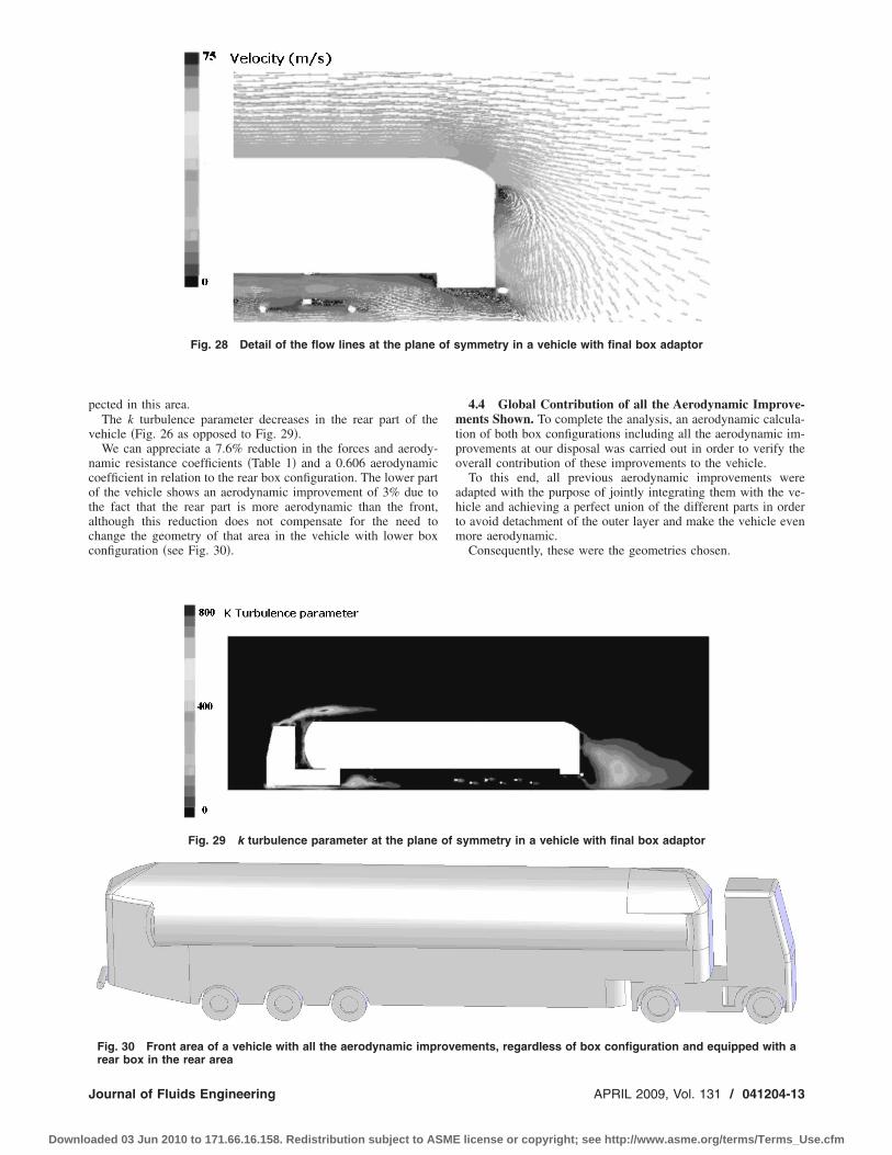
pected in this area.The k turbulence parameter decreases in the rear part of the

vehicle �Fig. 26 as opposed to Fig. 29�.We can appreciate a 7.6% reduction in the forces and aerody-

namic resistance coefficients �Table 1� and a 0.606 aerodynamiccoefficient in relation to the rear box configuration. The lower partof the vehicle shows an aerodynamic improvement of 3% due tothe fact that the rear part is more aerodynamic than the front,although this reduction does not compensate for the need tochange the geometry of that area in the vehicle with lower boxconfiguration �see Fig. 30�.

4.4 Global Contribution of all the Aerodynamic Improve-ments Shown. To complete the analysis, an aerodynamic calcula-tion of both box configurations including all the aerodynamic im-provements at our disposal was carried out in order to verify theoverall contribution of these improvements to the vehicle.

To this end, all previous aerodynamic improvements wereadapted with the purpose of jointly integrating them with the ve-hicle and achieving a perfect union of the different parts in orderto avoid detachment of the outer layer and make the vehicle evenmore aerodynamic.

Consequently, these were the geometries chosen.

Fig. 28 Detail of the flow lines at the plane of symmetry in a vehicle with final box adaptor

Fig. 29 k turbulence parameter at the plane of symmetry in a vehicle with final box adaptor

Fig. 30 Front area of a vehicle with all the aerodynamic improvements, regardless of box configuration and equipped with arear box in the rear area



If we examine the results obtained for the lower box configu-ration, we find a 0.52 aerodynamic coefficient, i.e., 15.85% less,due both to the contribution of the undercarriage skirt and that ofthe aerodynamic front, as well as to the joint integration of bothelements. This can be appreciated in Figs. 31–33, in which wemay notice the reduction of the k vorticity parameter in the un-dercarriage skirt area and the king-pin cavity. We also notice themovement of particles, which tends to produce less vortices and,consequently, to generate less turbulence. Thus the aerodynamicimprovements are expected to prove effective �see Table 1�.

The implementation of all the aerodynamic improvements forthe rear box configuration yields a 0.505 aerodynamic coefficient,i.e., 23% less in relation to the original rear box configuration, asmight have been expected �see Fig. 34�. This aerodynamic coef-ficient is noticeably inferior to that of the vehicle with the lowerbox configuration including all the aerodynamic improvements,due to the fact that the configuration used for the rear box is moreaerodynamic, although the improvement obtained amounted onlyto 3%.

As far as turbulence is concerned, and as a result of the aero-dynamic improvements implemented in these areas, we notice adecrease in the value of the k turbulence parameter in the slip-stream, the wheel area and the king-pin cavity �Fig. 33 versus Fig.

14�.We may also notice, in Fig. 35 versus Fig. 13, that there are less

vortices in the flow lines and that flow is redirected.Figures 33 and 36 �versus Fig. 13� shows that the turbulence in

the bottom zone and in the wheel zone of the trailer has beenreduced, because the underskirt decreases the geometry changesand redirects the air flow properly �see Figs. 32 and 35 versus Fig.13�.

5 Economical AnalysisAll the improvements that have been used in the cryogenic

tanker trailer can be used in any type of tanker trailer without theneed to make any modification, so the analysis that has been doneis for all types of tankers. The benefit of these improvements isclear regardless of the vehicle tanker, but the percentage canchange depending on the geometry of the tanker. In this paper astandard tanker has been used.

To know if the improvements are viable it is essential to makean economic analysis of them in the US market, so we have usedthe NADA �21,22,25� database and the “Truck Inventory Use andSurvey” �26�. They indicate that in 2003 there were, in USA,85,174,800 trailers and out of them 34,056,134 were tanker trail-

Fig. 31 Speed at the plane of symmetry in a vehicle with lower box configuration and all theimprovements

Fig. 32 Flow lines on a vertical plane 1 m above the ground in a vehicle with lower boxconfiguration and all the improvements



ers. For the cost analysis a price of 2.1 $/gal �11/09/2008� hasbeen used and a vehicle consumption of 16 gal/100 miles and100.000 miles/year for a standard vehicle. This indicates an an-nual consumption of 16,000 gal and a cost of 33,600 $/year. Asfor the improvements, the repercussion of them on the consumer

depends on some factors �average speed, driving style, orography,etc., but can vary from 10% for slow trailers to 50% for trailersthat make railway routs. 40% has been used�. The potential costshave been estimated �see Table 2�.

The economic results show that with low cost �less than $1100�

Fig. 33 k turbulence parameter at the plane of symmetry in a vehicle with a lower box and theimprovements

Fig. 34 Speed at the plane of symmetry in a vehicle with rear box configuration and all theimprovements

Fig. 35 Flow lines on a vertical plane 1 m above the ground in a vehicle with a rear box and allthe improvements



the fuel consumption is cut down and the annual saving can be$2100, so the return on investment �ROI� is approximately 0.5years and the economic gain is clearly large. �all economic resultsare in Table 2�. There are also environmental benefits with theCO2 emissions being reduced by 2.73 Tm during a year.

6 ConclusionsFollowing a detailed analysis of the results obtained and the

methodology implemented, the conclusion reached was that CFDprograms are very useful tools for performing aerodynamic modi-fications in vehicles at a very low cost, and that they allow theachievement of satisfactory results in a short period of time.

There is a wide field of research and a number of improvementsto be explored as far as aerodynamic improvements in articulatedtanker-type semitrailers are concerned. This is due to the fact thatlatter-day vehicles have few or no aerodynamic improvementsowing to the small amount of research carried out in this transportsector. Therefore, bearing in mind the results obtained and thefuture prospects of reducing fuel consumption in vehicles, thisfield of research would seem most promising.

It must be pointed out that the coefficient of aerodynamic re-sistance can be considerably lowered without modifying the di-mensions of the elements subject to mechanical stress by addingexternal aerodynamic elements that do not entail substantialweight penalization, such as those included in this chapter. Thusthe vehicles presently being used can implement these improve-ments to reduce fuel consumption and improve energy efficiencywithout having to resort to far-reaching modifications.

In relation to the aerodynamic improvements introduced, it isworth pointing out that the aerodynamic skirt entails the greatestaerodynamic gain of all, and involves a 9% improvement in theaerodynamic coefficient, by preventing the flow of air toward thelower part of the vehicle, where turbulence is predominant.

The contribution of the remaining aerodynamic improvementsis also relevant, and their use is always advantageous �see Table1�, although the undercarriage skirt is preferable as an initial aero-dynamic improvement. Should the others be implemented as well,they ought to be integrated with the use of the skirt. The integrateduse of all these improvements can lead to an aerodynamic im-provement of up to 23%, which would measure up to an improve-ment of up to 11% in fuel consumption. Although this comesclose to the 15% expounded in Sec. 1, it does not include im-provements in the tractor or those improvements due to modifica-tions in the shape of the resistant elements, which may make upfor that 4% difference.

Last but not the least relating to the economic aspect, the aero-dynamical improvements have a ROI of 0.5 years and the eco-nomic benefit is clearly substantial.

References�1� Morelli, A., 2000, “A New Aerodynamic Approach to Advanced Automobile

Basic Shapes,” SAE Technical Paper No. 2000-01-0491, p. 104.�2� Wood, R. M., and Bauer, S. X. S., 2003, “Simple and Low Cost Aerodynamic

Drag Reduction Devices for Tractor-Trailer Trucks,” SAE Paper No. 2003-01-3377.

�3� Bachman, L. J., Erb, A., and Bynum, C. L., 2005, “Effect of Single Wide Tiresand Trailer Aerodynamics on Fuel Economy and NOx Emissions of Class 8Line-Haul Tractor ,” SAE Paper No. 05CV45.

�4� Rutledge, W. H., Polansky, G. F., and Clark, E.L., 1988, “Aerodynamic Designand Performance of a Bent-Axis Geometry Vehicle,” J. Spacecr. Rockets,25�4�, pp. 257–262.

�5� Wood, R. M., 2004, Advanced Aerodynamic Trailer Technology.�6� 2007, FreightWing’s web page, http://www.freightwing.com�7� 2007, Nosecone’s web page, http://www.nosecone.com�8� Graham, S., and Bigatel, P., 2001, “Freight Wing Trailer Aerodynamics,” Tech-

nical Report No. JA-132.�9� Kleber, A., 2005, “Simulation of Air Flow Around an OPEL Astra Vehicle

With Fluent,” International Technical Development Center, Adam, Opel AG,Journal Articles by FLUENT Software users, www.fluent.com/solutions/articles/ja132.pdf

Table 2 Economical analysis of the improvements

Fig. 36 k turbulence parameter on a vertical plane 1 m above the ground in a vehicle with arear box and improvements



�10� Saiz, V., 2005, “Estudi i Simulació Aerodinàmica del Roadster FS1,” MSthesis, Escola Tècnica d’Enginyers Industrials de Barcelona, Barcelona, Spain.

�11� ROS ROCA INDOX CryoEnergy, http://www.cryoenergy.net�12� Canet, J. M., Bugeda, G., and Oñate, E., 1991, Simulación Numérica de la

Aerodinámica de Vehículos, Centro Internacional de Métodos Numéricos enIngeniería, Barcelona, Spain.

�13� 2004, FLUENT 6.2 Documentation, User’s Guide, Fluent, Inc.�14� Parneix, S., Durbin, P. A., and Behnia, M., 1998, “Computation of 3-D Tur-

bulent Boundary Layer Using theV2 Model,” Flow, Turbul. Combust., 60, pp.19–46.

�15� Menter, F. R., 1994, “Two-Equation Eddy-Viscosity Turbulence Models forEngineering Applications,” AIAA J., 32�8�, pp. 1598–1605.

�16� Davidson, L., 2003, An Introduction to Turbulence Models, Chalmers Univer-sity of Technology, Reston, VA.

�17� Durbin, P. A., 1991, “Near-Wall Turbulence Closure Modelling Without‘Damping Functions’,” Theor. Comput. Fluid Dyn., 3, pp. 1–13.

�18� Mercker, E., and Knape, H. W., 1989, “Ground Simulation With Moving Belt

and Tangential Blowing for Full-Scale Automotive Testing in a Wind Tunnel,”SAE Paper No. 890367.

�19� Skea, A. F., Bullen, P. R., and Qiao, J., 1998, “The Use of CFD to Predict theAir Flow Around a Rotating Wheel,” MIRA, International Symposium onAutomotives Technology and Automation, Düsseldorf, Germany.

�20� Wong, J. Y., 1993, Theory of Ground Vehicles, 2nd ed., Wiley, Ottawa, Canada.�21� Carr, G. W., 1983, “Potential for Aerodynamic Drag Reduction in Car De-

sign,” Int. J. Veh. Des., pp. 51–52.�22� Carr, G. W., 1983, “Potential for Aerodynamic Drag Reduction in Car De-

sign,” Int. J. Veh. Des., pp. 176–196.�23� Heisler, H., 2002, Advanced Vehicle Technology, 2nd ed., Butterworth–

Heinemann, Oxford, pp. 584–617.�24� Comisión Nacional para el Ahorro de Energía de México �Mexico D.C.,

Mexico�, 2007, www.conae.gob.mx�25� National Automobile Dealers Association, http://www.nada.org/�26� U.S. Census Bureau, “Truck Inventory and Use Survey,” http://

www.census.gov/svsd/www/tiusview.html

Dr. Ramon Miralbes Buil obtained a degree in Industrial Engineering from Zaragoza University in 2005 (Spain), with specializationin Vehicle and Machinery Design. From this time on, he continued his Ph.D. studies in the area of New Materials for Road Transportin this university. In February 2008 he finished his Ph.D. studies with the thesis: “Flow-Termo-Mechanical Analysis of CryogenicTanker Vehicles” and is working on several research projects involving vehicle strength and rigidity performance simulation by theFEM. He also works as an Associate Professor in the area of Design and Graphic Expression at the University of Zaragoza.

Dr. Luis Castejon Herrer graduated with a degree in Mechanical Engineering (University of Zaragoza, Spain, 1992) and a Ph.D. inMechanical Engineering (University of Zaragoza, Spain, 1998). Dr. Luis Castejon Herrer is a full Professor in Transportation Engi-neering at the University of Zaragoza. Since 1991, he has been involved in several projects in the areas of Vehicle Dynamics and NewMaterials for vehicles, buses, railways, and ground transportation. He has written over 120 papers in technical journals and interna-tional congresses and 9 books, published in Europe. He has been a researcher in the European BRITE-EURAM Project “MULTEX-COMP” and he has collaborated in other European projects such as “SEABUS” and “AFICOSS.” He has participated in several R+DSpanish projects. He developed his Ph.D. thesis on the simulation of roll over of metallic and composite buses by means of FEM,obtaining the Doctoral Special Award of the University of Zaragoza.



R. W. Hewson1

School of Mechanical Engineering,University of Leeds,

Woodhouse Lane,Leeds, LS2 9JT UK


Free Surface Model Derived Fromthe Analytical Solution of StokesFlow in a WedgeThe formation of a thin liquid film onto a moving substrate is a commonly encounteredindustrial process, and one that is encountered in lubrication, oil extraction processes,and coating flows. The formation of such a film is analyzed via the analytical Stokes flowsolution for the flow in a wedge bounded on one side by a free surface and on the otherby a moving surface. The full solution is obtained by numerically integrating a set ofordinary differential equations from far downstream, in the region of the final film thick-ness. The results show excellent agreement with the results obtained by the Brethertonequation, the Ruschak equation, the Coyne and Elrod model, and a two-dimensional freesurface finite element simulation of the problem. �DOI: 10.1115/1.3089540�

1 IntroductionThe deposition of a thin liquid film is commonly encountered in

a number of tribological and coating applications �1–3� and in-volves the deposition of the thin film onto a moving substrate as itsweeps from a fluid filled gap, as shown in Fig. 1. As such therehave been a number of analyses of the problem, most notably thatof Bretherton �4� �see also Ref. �5�� who, using a similar methodof matched asymptotic expansion as Landau and Levich �6�, de-termined the residual fluid deposited onto a moving substrate by,

h0

r= 1.337Ca2/3, Ca � �0,10−2� �1�

where h0 is the residual film thickness, r is the �constant� menis-cus radius, and Ca is the capillary number given by Ca=�U /� ��is the fluid viscosity, U is the substrate speed, and � is the inter-facial surface tension�.

Ruschak �7� used the finite element method �FEM� to obtain anempirical expression governing the residual film thickness to gapratio for higher capillary numbers than those for which theBretherton expression is valid.

h0

h�=�

= 0.54�Ca, Ca � �10−2,10−1� �2�

where h�=� is the initial fluid filled gap. One limitation of Rus-chak’s equation is that although it predicts the residual film thick-ness accurately, the nonconstant meniscus radius means that Eq.�2� is not able to calculate the local pressure at the point of filmformation, an important parameter, and one that is often used as apressure boundary condition in a range of different coating andlubrication problems. This is noted by Thompson et al. �8� whocompared the finite element method with the lubrication approxi-mation for reservoir fed rigid roll coating.

Coyne and Elrod �9� derived a set of four ordinary differentialequations �ODEs� to describe the process of film formation bysolving the Navier–Stokes equations along the free surface. Themodel assumes a quadratic velocity profile to describe the flowperpendicular to the free surface. One limitation of the model isthe stiffness of the set of equations around the free surface stag-nation point �occurring at 3H�. Despite this, the method has beenused by some investigators as a free surface boundary condition

for lubrication �3� �via a function fitted to the data in Coyne andElrod’s paper �9�� as well as for coating problems �2,7�.

The cavitation boundary condition can have a significant effecton the pressure profile within the lubricated geometry studied�10�. In addition to the film splitting model described here, thereare a number of other models that can be applied to lubricationflows to describe the film splitting process, these include theSwift–Steiber condition �11� and the Prandtl–Hopkins condition�12,13� �u=du /dx=0� �as examined for the case of roll coating bySavage �14��.

Hewson et al. �15� solved the film forming problem as a bound-ary value problem �BVP� for shear thinning fluids obeying boththe power law and the Ellis fluid models. The results for the New-tonian fluids �power index n=1� compared well with those of theCoyne and Elrod model and the Bretherton and Ruschak equa-tions within their ranges of applicability. The model describedhere is an attempt to provide a solution to the film forming prob-lem, in a similar way to that of Coyne and Elrod �i.e., the numeri-cal solution of ODEs� using equations that are computationallymore stable, in doing so the film forming process has been de-scribed for a range of capillary numbers and contact angles. Theprimary difference between the model presented here and that ofCoyne and Elrod is that the flow described here is based on thesolution of Stokes flow in a wedge type geometry rather than as aquadratic velocity profile perpendicular to the free surface �as isconsistent with the lubrication approximation�.

2 Model FormulationThe problem is solved using an analysis similar to that of the

long wave approximation but with the local flow solution basedon the Stokes solution for the flow in a wedge shaped geometry.For such an assumption to be strictly valid, the free surface radiusof curvature must be greater than the residual film thickness�16�—in addition to the work of Snoeijer the analysis here uses asimilar method to that of Cox �17,18�. This is valid in the regionwhere the free surface is close to the moving substrate—i.e., in theregion where viscous forces are greatest �4�. In undertaking theanalysis the variation in film thickness in the region where the freesurface is close to the moving substrate is taken into account indetermining the free surface profile.

The solution of Stokes flow in a wedgelike geometry with onefree surface, one moving surface, and a net flux is formulated inpolar coordinates and solved in terms of the stream function �, asfollows:


JOURNAL OF FLUIDS ENGINEERING. Manuscript received July 24, 2008; final manuscriptreceived January 15, 2009; published online March 11, 2009. Assoc. Editor: MalcolmJ. Andrews.



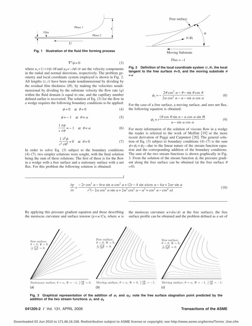
�4� = 0 �3�

where ur=1 /r�� /�� and u�=−�� /�r are the velocity componentsin the radial and normal directions, respectively. The problem ge-ometry and local coordinate system employed is shown in Fig. 2.All lengths �x ,r� have been made nondimensional by dividing bythe residual film thickness �H�, by making the velocities nondi-mensional by dividing by the substrate velocity the flow rate �q�within the fluid domain is equal to one, and the capillary numberdefined earlier is recovered. The solution of Eq. �3� for the flow ina wedge requires the following boundary conditions to be applied:

� = 0 at � = 0 �4�

� = − 1 at � = � �5�

1

r

��

��= − 1 at � = � �6�

1

r2

�2�

��2 = 0 at � = 0 �7�

In order to solve Eq. �3� subject to the boundary conditions�4�–�7�, two simpler solutions were sought, with the final solutionbeing the sum of these solutions. The first of these is for the flowin a wedge with a free surface and a stationary surface with a netflux. For this problem the following solution is obtained:

�1 = −2� cos2 � − � − sin � cos �

2� cos2 � − � − sin � cos ��8�

For the case of a free surface, a moving surface, and zero net flux,the following equation is obtained:

�2 = r�� cos � sin � − � cos � sin ��

� − sin � cos ��9�

For more information of the solution of viscous flow in a wedgethe reader is referred to the work of Moffatt �19� or the morerecent derivation of Paggi and Carpinteri �20�. The general solu-tion of Eq. �3� subject to boundary conditions �4�–�7� is the sum�=�1+�2—due to the linear nature of the stream function equa-tion and the corresponding addition of the boundary conditions.The sum of the two stream functions is shown graphically in Fig.3. From the solution of the stream function �, the pressure gradi-ent along the free surface can be obtained �at the free surface �=0�.

�p

�r=

− 2r cos3 � − 4r� sin � cos2 � + �2r − 4 sin ��cos � − 4� + 2�r sin �

r3�− 2� cos3 � sin � + 2�2 cos2 � − �2 + cos2 � − cos4 ��10�

By applying this pressure gradient equation and those describingthe meniscus curvature and surface tension �p=� /Ca, where � is

the meniscus curvature �=d� /ds at the free surface�, the freesurface profile can be obtained and the problem defined as a set of

HPhase 2

U

FilmCPhase 1

Fig. 1 Illustration of the fluid film forming process

Flux = −1

α(r,θ)

Free surface

Moving Substrate

Fig. 2 Definition of the local coordinate system „r ,�…, the localtangent to the free surface �=0, and the moving substrate �=�

Free surface,θ = 0, Ψ = 0,1r2

∂2Ψ∂θ2 = 0.

Stationary surface, θ = α, Ψ = −1, 1r

∂Ψ∂θ = 0.


∂2Ψ∂θ2 = 0.

Moving surface, θ = α, Ψ = 0, 1r

∂Ψ∂θ = −1.


∂2Ψ∂θ2 = 0.

Moving surface, θ = α, Ψ = −1, 1r

∂Ψ∂θ = −1.

(a) (b) (c)

Fig. 3 Graphical representation of the addition of �1 and �2: note the free surface stagnation point predicted by theaddition of the two stream functions �1 and �2



four first order ODEs �with respect to distance along the freesurface s�, one of which is Eq. �10� ��p /�r=dp /ds�, the otherthree are as follows:

d�

ds= − Cap �11�

dh

ds= sin�� 12�

dx

ds= cos�� 13�

where h is the film thickness perpendicular to the substrate, and xis the distance along the substrate from the initial condition. Equa-tion �13� is not required in order to close the problem but providesinformation on the distance downstream from the origin, allowingthe meniscus shape to be determined. In addition to the four ODEsthe identity r=h /sin � is also used. The set of four ODEs weresolved using MATLAB’s general ODE solver ode45 and were inte-grated from downstream, in the final film region to an angle of�=90 deg �however different limits of � can be used ifrequired—as determined by the contact angle�. It should also benoted that it is possible to solve the set of equations as a BVP withthe option of using a further equation �dq /ds=0� describing theflux if this is to be solved for. For this approach the reader isreferred to Ref. �15�. The initial conditions used are characteristicof the final film thickness with a perturbation applied to the freesurface angle ��=10−5 rad�. These initial conditions allow stableperturbation independent solutions to be obtained. The model de-tailed here has the advantage over the widely used analysis ofCoyne and Elrod �9�, in that the instability in obtaining their so-lution is not present in this analysis. As the solution is obtained

(a)

(b)

Fig. 4 COMSOL MULTIPHYSICS finite element implementation of thefree surface problem

−100 −80 −60 −40 −20 0−20

−10

0

10

20

30

40

50

60

70

80

x

Model Free SurfaceConstant radiusPressureFE Free Surface

(a)−30 −25 −20 −15 −10 −5 0

−10

−5

0

5

10

15

20

x(b)

−12 −10 −8 −6 −4 −2 0−3

−2

−1

0

1

2

3

4

5

6

x(c)−5 −4 −3 −2 −1 0

−1

−0.5

0

0.5

1

1.5

2

2.5

3

x(d)

Fig. 5 Free surface meniscus shape, pressure distribution and constant radius at �=90 deg, as obtained by the analyticalmodel „Eqs. „10…–„13……



using numerical integration rather than by solving the problem asa BVP as in the analysis of Hewson et al., the model is memoryand time efficient and allows the model to be applied to a widerange of coating type flows.

2.1 FEM. The FEM was used to compare with the modelresults. The simulation was undertaken in COMSOL MULTIPHYSICS

using the arbitrary Lagrangian Eulerian �ALE� method. The fluidwas modeled as Stokes flow with the free surface curvature ob-tained by calculating the rate of change with distance along thefree surface of the angle the free surface makes with the movingsubstrate �an implementation that can be achieved in COMSOL bydefining the free surface angle as an additional variable along theboundary�. The simulation used to obtain the results had27,733DOF and solution times were of the order of 10 min; themesh and an example solution are shown in Fig. 4. The velocityinlet boundary condition on the left hand side of the domain isquadratic, consistent with the lubrication approximation. The flowrate across this boundary was varied until the angle the free sur-face made with the symmetry boundary condition �along the topof the domain� was 90 deg. The main results extracted from theFEM simulations where the final film thickness and the free sur-face profile. To facilitate the analysis the final film thickness wassolved for with the gap h�=� kept fixed, this is accounted for inSec. 3 were the results have been appropriately scaled.

3 Results and DiscussionFigure 5 shows the free surface profile for a range of different

capillary numbers; also plotted is a constant radius based on thecurvature at �=90 deg. It is interesting to note that as the capil-lary number decreases then as would be expected, the meniscusshape follows the constant radius more closely and that the greaterthe viscous forces, the greater the proportion of the meniscus thatis not constant in radius. For capillary numbers of Ca=0.001 andCa=0.01, the finite element and model results are almost identical�the finite element results line is obscured by the free surface lineobtained from the model�. For a capillary number of Ca=0.1 thereis still good agreement between the model and the finite elementresults, with the model capturing the divergence from the constantradius reasonably well. However, for a capillary number of Ca=1 the results diverge significantly.

Perhaps the results of greatest interest are those of the final filmthickness and the meniscus curvature—which allows the localpressure to be determined and can be applied as a boundary con-dition in a range of different lubrication analyses. Here a compari-son is made with the results of the Bretherton equation, Ruschak’sequation, and the numerical results of Coyne and Elrod as well asthe FEM.

Figure 6�a� shows how the residual film thickness varies withcapillary number. It can be seen that these results are in excellentagreement with one another. Comparing the radius of curvature tofilm thickness ratio at �=90 deg �Fig. 6�b�� shows general agree-ment for capillary numbers below Ca=0.1 �if a constant meniscusradius is assumed for Ruschak’s model a constant radius of cur-vature of unity would result due to the choice of scaling em-ployed�. It can be seen that both the model described here and thatof Coyne and Elrod both represent the free surface curvature forlow capillary numbers reasonably well. The model described heremore closely follows the finite element results for capillary num-bers below Ca�0.1 however the Coyne and Elrod model is moreaccurate as the capillary number increases further.

The reducing accuracy of the model for higher capillary num-bers is consistent with the observation that the analysis is valid forthe location where the free surface radius of curvature is largerelative to the film thickness. This is in agreement with the analy-sis of Bretherton �4�, however unlike the analysis of Brethertonthe divergence from a constant radius is accounted for, alluding to

the possibility that the analysis may be able to predict the filmprofile at higher capillary numbers—something already shown byexamining the free surface profile data.

4 ConclusionsThe model detailed here provides an accurate and reasonably

efficient means of calculating the free surface shape of a fluid filmdrawn from a gap. The method is more stable than that developedby Coyne and Elrod and allows greater capillary numbers to beinvestigated than the simpler relationships developed by Brether-ton and Ruschak. It should be noted that there is some additionalcomputational cost associated with the solution, when comparedwith the elegant solution of Bretherton so a compromise betweencomputational cost and accuracy at moderately high capillarynumbers must be borne in mind when deciding on the free surfacemodel to adopt. However the model outlined here provides anextension to higher capillary numbers compared with the Brether-ton equation, with the results showing that a capillary number ofCa=0.1 is a realistic upper limit for the model.

AcknowledgmentIt is a pleasure to acknowledge Yeaw Chu Lee for his interest-

ing discussions on Stokes flow.

References�1� Greener, J., and Middleman, S., 1979, “Theoretical and Experimental Studies

10−3

10−2

10−1

100

100

101

102

Capillary number, Ca

C

ODEBrethertonRuschakCEFEM

(a)

10−3

10−2

10−1

100

0.4

0.5

0.6

0.7

0.8

0.9

1

Capillary number, Ca

(dθ/

ds)/

(C−

1)

ODECEFEM

(b)

Fig. 6 Results of the model, compared with Bretherton equa-tion, Ruschak equation, and Coyne and Elrod „CE… results; for„a… gap, h�=0 „at �=90 deg… and „b… scaled meniscus radius ofcurvature d� /ds / „h�=�−1…



of the Fluid Dynamics of a Two-Roll Coater,” Ind. Eng. Chem. Fundam.,18�1�, pp. 35–41.

�2� Benkreira, H., Edwards, M. F., and Wilkinson, W. L., 1982, “Ribbing Instabil-ity in the Roll Coating of Newtonian Fluids,” Plastics and Rubber Processingand Applications, 2, pp. 137–144.

�3� Priest, M., Dowson, D., and Taylor, C. M., 2000, “Theoretical Modelling ofCavitation in Piston Ring Lubrication,” Proc. Inst. Mech. Eng., Part C: J.Mech. Eng. Sci., 214�3�, pp. 435–447.

�4� Bretherton, F., 1961, “The Motion of Long Bubbles in Tubes,” J. Fluid Mech.,10, pp. 166–168.

�5� Park, C. W., and Homsy, G. M., 1984, “Two-Phase Displacement in HeleShaw Cells: Theory,” J. Fluid Mech., 139, pp. 291–308.

�6� Landau, L., and Levich, B., 1942, “Dragging of a Liquid by a Moving Plate,”Acta Physicochim. URSS, 17, pp. 42–54.

�7� Ruschak, K. J., 1982, “Boundary-Conditions at a Liquid Air Interface in Lu-brication Flows,” J. Fluid Mech., 119, pp. 107–120.

�8� Thompson, H. M., Kapur, N., Gaskell, P. H., Summers, J. L., and Abbott, S. J.,2001, “A Theoretical and Experimental Investigation of Reservoir-Fed, Rigid-Roll Coating,” Chem. Eng. Sci., 56�15�, pp. 4627–4641.

�9� Coyne, J. C., and Elrod, H. G., 1970, “Conditions for the Rupture of a Lubri-cating Film. Part 1: Theoretical Model,” ASME J. Lubr. Technol., 92, pp.451–456.

�10� Cameron, A., 1979, Basic Lubrication Theory, Longman, Greens, New York.�11� Swift, H. W., 1932, “The Stability of Lubricating Films in Journal Bearings,”

Proc. Inst. of Civ. Eng. �UK�, 233, pp. 267–288.�12� Prandtl, L., 1928, “Motion of Fluids With Very Little Viscosity,” Technical

Memorandum of the National Advisory Committee, NACA.�13� Hopkins, M. R., 1957, “Viscous Flow Between Rotating Cylinders and a Sheet

Moving Between Them,” Br. J. Appl. Phys., 8, pp. 442–444.�14� Savage, M. D., 1982, “Mathematical-Models for Coating Processes,” J. Fluid

Mech., 117, pp. 443–455.�15� Hewson, R. W., Kapur, N., and Gaskell, P. H., 2005, “Film Formation Model

of Shear Thinning Power Law Fluids Using Lubrication Analysis,” EuropeanCoating Symposium, Bradford, West Yorkshire.

�16� Snoeijer, J. H., 2006, “Free-Surface Flows With Large Slopes: Beyond Lubri-cation Theory,” Phys. Fluids, 18�2�, pp. 021701.

�17� Cox, R. G., 1986, “The Dynamics of the Spreading of Liquids on a Solid-Surface. Part 1. Viscous-Flow,” J. Fluid Mech., 168, pp. 169–194.

�18� Boender, W., Chesters, A. K., and Vanderzanden, A. J. J., 1991, “An Approxi-mate Analytical Solution of the Hydrodynamic Problem Associated With anAdvancing Liquid Gas Contact Line,” Int. J. Multiphase Flow, 17�5�, pp.661–676.

�19� Moffatt, H. K., 1964, “Viscous and Resistive Eddies Near a Sharp Corner,” J.Fluid Mech., 18�1�, pp. 1–18.

�20� Paggi, M., and Carpinteri, A., 2008, “On the Stress Singularities at Multima-terial Interfaces and Related Analogies With Fluid Dynamics and Diffusion,”Appl. Mech. Rev., 61�2�, pp. 020801.



Włodzimierz Wróblewskie-mail: [email protected]

Sławomir Dykas

Institute of Power Engineering andTurbomachinery,

Silesian University of Technology,Gliwice, Poland

Andrzej GardzilewiczInstitute of Fluid-Flow Machinery,

Polish Academy of Science,Gdansk, Poland


Michal KolovratnikCzech Technical University in Prague (CTU),

Prague, Czech Republice-mail: [email protected]

Numerical and ExperimentalInvestigations of SteamCondensation in LP Part of aLarge Power TurbineThis paper presents the experimental investigations of steam flow with condensation inthe blading system of the low-pressure (LP) part of a 360 MW turbine. To this end,special probes were used, which provided flow visualization opportunities including lo-calization of the front of condensation, determining distributions of pressure, tempera-ture, velocity, and flow angle in the inter-row gaps, measurements of water droplet con-centration and sizes. The measurements have proved that the condensation process in theLP turbine might be of heterogeneous nature, depending on the concentration of chemicalimpurities in steam. The measurement results constituted the basis for computational fluiddynamics (CFD) flow calculations, which were performed using the time-dependent 3DReynolds averaged Navier–Stokes equations coupled with two-equation turbulence model(k-� SST) and additional conservation equations for the liquid phase. The set of govern-ing equations has been closed by a “local” real gas equation of state. The condensationphenomena were modeled on the basis of the classical nucleation theory. The heteroge-neous condensation model on the insoluble and soluble impurities was implemented intopresented CFD code. The system of governing equations was solved by means of a finitevolume method on a multiblock structured grid. The obtained numerical results andexperimental data were compared and discussed. �DOI: 10.1115/1.3089544�

1 IntroductionThe flow of steam through the blades of a low-pressure �LP�

turbine results in condensation that unfavorably influences effi-ciency of power generation. The homogeneous condensation insteam flow occurs when there are no foreign nuclei. In real con-ditions, for steam power cycle, the steam always contains someimpurities of both insoluble and soluble characters. Therefore, inreal turbine, the wetness appears as a result of a mixedhomogeneous/heterogeneous condensation or pure heterogeneouscondensation, everything depends on the quantity of foreign nu-clei.

The lack of experimental data for the steam flow with hetero-geneous condensation and new data for the flow with pure homo-geneous condensation limit the progress in numerical modeling ofthe wet steam flows. It is very difficult to reproduce the real con-ditions in large output turbine in experiment; it refers to the flowconditions and steam quality, the number, and the sort of the im-purities. The impurities may change the mechanism of the liquidphase generation and may intensify the corrosion and erosion pro-cesses. Many operational experiences in the power plants �e.g.,Refs. �1,2�� and author’s own observations confirm that facts.

In the feedwater cycle of power plant, different sources of im-purities may be identified: mechanical, chemical, or electrochemi-cal ones. Particles that exist in steam are soluble and insolublecompounds �salts and alkalis�. For the parameter range occurringin water-steam cycle, these impurities can be divided into groupswith and without phase change. In the first group, sodium chloride�NaCl� is the most important one, taking into consideration con-densation process, which dissolves just above the saturation lineof pure steam. As regards condensation on soluble particles, it is

necessary to take into account the size change of the particles andthe solution concentration in the droplets. The condensation modelrequires knowledge of many physical and chemical properties ofthe salt solution in steam. It is often very hard to find enoughinformation in the references, as well as from the feedwater analy-sis in the power plant.

Two processes have to be considered during steam expansion inthe turbine: homogeneous and heterogeneous condensations.Steam impurities, necessary to initiate heterogeneous condensa-tion, occur in the form of suspension of particles, which are in-soluble or soluble in water. The chemical and physical propertiesof a suspension influence the size of the droplets nucleated on theparticles and the nucleation process.

It is possible to model various types of condensation processes,i.e., homogeneous and heterogeneous ones �on soluble and in-soluble particles�. The necessary step in the nonequilibrium wetsteam flow modeling is the validation of the numerical modelsagainst the experimental results. The development of numericalmethods for wet steam flow calculations has to allow for real gasproperties, which, in fact, is the fundamental one for correct cal-culations of the condensation process. The correct calculation ofthe steam flow for low pressures close to the saturation line andfor high pressures needs to implement the real gas equation ofstate into numerical algorithm. The relation between thermal pa-rameters of state is nonlinear within these ranges and does notfollow the ideal equation of state. Moreover, in the case of wetsteam, a two-phase flow model has to be considered.

The developed steam condensing flow models have been vali-dated against experimental data for simple 2D test cases. Usually,they are the Laval nozzles in which 1D flow form dominates. Allavailable experimental investigations relate to the homogeneouscondensation, whereas in real turbine the heterogeneous conden-sation is predominant. Therefore, validation of the numerical al-gorithm for modeling the flow in real turbine stages by means ofsuch test cases is not easy; it has been discussed in Refs. �3,4�.

The comparison of the numerical modeling and measurements

Contributed by the Fluids Engineering Division of ASME for publication in theJOURNAL OF FLUIDS ENGINEERING. Manuscript received October 30, 2007; final manu-script received October 6, 2008; published online March 9, 2009. Assoc. Editor:Chunill Hah.



of the flow in real turbine of the large output is not often pub-lished. The crucial value of such verification comes down to theassessment of flow conditions for real LP steam turbine stages bymeans of the CFD code.

This paper presents the results of experimental and numericalinvestigations of 3D flows through the last two stages of the LPpart of a 360 MW turbine. The problems of condensation in a LPsteam turbine has been presented and discussed also, e.g., byHesler et al. �5�, Bakhtar and Heaton �6�, and Petr et al. �7�.

Measurements of thermodynamic parameters, the size, and con-centration of water droplets together with CFD results have beendescribed below. The presented work was performed by researchteams of the Institute of Fluid-Flow Machinery from Gdansk �PL�,the Czech Technical University �CTU� of Prague, and the SilesianUniversity of Technology �PL� within the framework of the Re-search Project No. 3T10B04726 sponsored by the State Commit-tee for Scientific Research in Poland.

2 Physical and Mathematical Model

2.1 Governing Equations. All results presented in this paperwere obtained by means of the in-house CFD code. The code isbased on the time-dependent 3D Reynolds averaged Navier–Stokes �RANS� equations formulated for the vapor/water mixture,which are coupled with a two-equation turbulence model �k-�SST model�, and with additional mass conservation equations forthe liquid phase: two for homogeneous condensation,

��yhom��t

+��yhomu�

�x+

��yhomv��y

+��yhomw�

�z

=4

3��l�r�3Jhom + 3�nhomrhom

2 drhom

dt�

�1��nhom�

�t+

��nhomu��x

+��nhomv�

�y+

��nhomw��z

= Jhom

and one for heterogeneous condensation:

��yhet��t

+��yhetu�

�x+

��yhetv��y

+��yhetw�

�z= 4��l�nhetrhet

2 drhet

dt

�2�

The droplet radius rhet in the heterogeneous condensation is cal-culated from the relation

rhet = �rp3 +

3

4�

yhet

�lnhet�1/3

�3�

where rp is the radius of the particle on which the droplet isgrowing.

For the two-phase nonequilibrium flow, it has been assumedthat the volume occupied by droplets is negligibly small. Theinteraction between droplets is not taken into account in themodel. The heat exchange between the liquid phase and the solidboundary, and the velocity slip between vapor and the liquidphase are neglected. The nonslip assumption is much less signifi-cant than the effects of the thermal nonequilibrium �8�. The con-servation equations are formulated for the two-phase mixture withthe specific parameters calculated with the following relations:

h = hv�1 − y� + h1y

s = sv�1 − y� + s1y �4�

� = �v/�1 − y�

The value of the nonequilibrium wetness fraction y is calculatedas the sum of the homogeneous and heterogeneous wetness ob-tained from the conservation equations for the liquid phase �1� and�2�.

2.2 Equation of State. For wet steam flow calculations, theset of ten governing equations has to be closed by a real gasequation of state �EOS�. The formulation of the real gas EOS iscompound even in case when simplified model has been used. Theidea of applied real gas EOS consisted in creation of equation ofstate with as simple mathematical form as possible, but simulta-neously very accurate. The simple mathematical form can be veryaccurate, but only within the small parameters range.

The mathematical form of used real gas EOS is similar to thevirial equation of state with one virial coefficient.

p�

RT= Z�T,�� = A�T� +

B�T��

�5�

where A�T� and B�T� are defined as

A�T� = a0 + a1T + a2T2

B�T� = b0 + b1T + b2T2

The coefficients ai ,bi�i=0, . . . ,2� of the polynomials A�T� andB�T� are the functions of temperature only, and they can be foundfrom an approximation of thermodynamic properties of steam cal-culated using IAPWS-IF’97 �9�. It is easily to notice that thisequation is represented by a relatively uncomplicated approximatesurface.

The equation of state �5� is called the “local” real gas equationof state because, due to the simple mathematical form, it can beapplied locally within the limited parameter range only.

Expressions for the specific enthalpy, specific entropy, andother properties such as specific heat capacities and speed ofsound can be determined from the standard thermodynamicrelations.

The concept of the local real gas equation of state can be ap-plied to determine the thermodynamic properties of any real gas,in the case when the simple mathematical form is needed.

2.3 Nucleation and Droplet Growth Model. The homoge-neous condensation phenomenon is modeled on the ground of theclassical nucleation theory of Volmer, Frenkel �10�, and Zeldovichand continuous droplet growth model of Gyarmathy �11�.

The nucleation rate, i.e., number of supercritical droplets pro-duced per unit mass of vapor per unit time, is calculated from therelation derived by the assumption of thermodynamic equilibriumbetween critical droplets and vapor. Additionally, the nonisother-mal correction factor C proposed by Kantrowitz �12� has beenused because the isothermal model assumption does not apply tothe vapor:

Jhom = C�2�

��1/2

mv−3/2�v

2

�lexp�− �

4�r�2�

3kTv� �6�

where coefficient C is calculated from the relation

C = �1 + 2� − 1

� + 1

hv − hl

RTv�hv − hl

RTv−

1

2��−1

and mv is the mass of a water molecule and � is the correctionfactor �in the calculations assumed=1�.

The radius of critical clusters r� for the applied real gas EOS �5�has a form that differs from the known relation for ideal gas:

r� =2�

�l�f�pv� − f�ps�� − �pv − ps��7�

where

f�p� =b

2ln p + c −

b

2ln 1 +

c

b

1 −c

b

b = A�T�RT



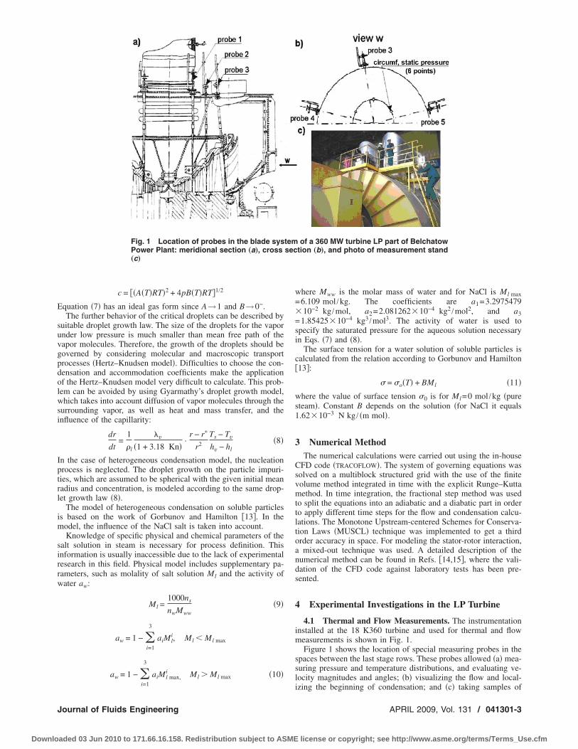
c = ��A�T�RT�2 + 4pB�T�RT�1/2

Equation �7� has an ideal gas form since A→1 and B→0−.The further behavior of the critical droplets can be described by

suitable droplet growth law. The size of the droplets for the vaporunder low pressure is much smaller than mean free path of thevapor molecules. Therefore, the growth of the droplets should begoverned by considering molecular and macroscopic transportprocesses �Hertz–Knudsen model�. Difficulties to choose the con-densation and accommodation coefficients make the applicationof the Hertz–Knudsen model very difficult to calculate. This prob-lem can be avoided by using Gyarmathy’s droplet growth model,which takes into account diffusion of vapor molecules through thesurrounding vapor, as well as heat and mass transfer, and theinfluence of the capillarity:

dr

dt=

1

�l

�v

�1 + 3.18 Kn�·

r − r�

r2

Ts − Tv

hv − hl�8�

In the case of heterogeneous condensation model, the nucleationprocess is neglected. The droplet growth on the particle impuri-ties, which are assumed to be spherical with the given initial meanradius and concentration, is modeled according to the same drop-let growth law �8�.

The model of heterogeneous condensation on soluble particlesis based on the work of Gorbunov and Hamilton �13�. In themodel, the influence of the NaCl salt is taken into account.

Knowledge of specific physical and chemical parameters of thesalt solution in steam is necessary for process definition. Thisinformation is usually inaccessible due to the lack of experimentalresearch in this field. Physical model includes supplementary pa-rameters, such as molality of salt solution Ml and the activity ofwater aw:

Ml =1000ns

nwMww�9�

aw = 1 − �i=1

3

aiMli, Ml Ml max

aw = 1 − �i=1

3

aiMl max,i Ml Ml max �10�

where Mww is the molar mass of water and for NaCl is Ml max=6.109 mol /kg. The coefficients are a1=3.2975479�10−2 kg /mol, a2=2.081262�10−4 kg2 /mol2, and a3=1.85425�10−4 kg3 /mol3. The activity of water is used tospecify the saturated pressure for the aqueous solution necessaryin Eqs. �7� and �8�.

The surface tension for a water solution of soluble particles iscalculated from the relation according to Gorbunov and Hamilton�13�:

� = �o�T� + BMl �11�

where the value of surface tension �0 is for Ml=0 mol /kg �puresteam�. Constant B depends on the solution �for NaCl it equals1.62�10−3 N kg / �m mol�.

3 Numerical MethodThe numerical calculations were carried out using the in-house

CFD code �TRACOFLOW�. The system of governing equations wassolved on a multiblock structured grid with the use of the finitevolume method integrated in time with the explicit Runge–Kuttamethod. In time integration, the fractional step method was usedto split the equations into an adiabatic and a diabatic part in orderto apply different time steps for the flow and condensation calcu-lations. The Monotone Upstream-centered Schemes for Conserva-tion Laws �MUSCL� technique was implemented to get a thirdorder accuracy in space. For modeling the stator-rotor interaction,a mixed-out technique was used. A detailed description of thenumerical method can be found in Refs. �14,15�, where the vali-dation of the CFD code against laboratory tests has been pre-sented.

4 Experimental Investigations in the LP Turbine

4.1 Thermal and Flow Measurements. The instrumentationinstalled at the 18 K360 turbine and used for thermal and flowmeasurements is shown in Fig. 1.

Figure 1 shows the location of special measuring probes in thespaces between the last stage rows. These probes allowed �a� mea-suring pressure and temperature distributions, and evaluating ve-locity magnitudes and angles; �b� visualizing the flow and local-izing the beginning of condensation; and �c� taking samples of

Fig. 1 Location of probes in the blade system of a 360 MW turbine LP part of BelchatowPower Plant: meridional section „a…, cross section „b…, and photo of measurement stand„c…



early condensate for chemical analyses.The probes can be mounted during nonstop operation into spe-

cial seats prepared during an overhaul of the turbine. The measur-ing probe, presented in Fig. 2, can be classified as a disk probe.This type is not sensitive to water films that form on it �16�. Theprobe tip consists of four �five� Pitot tubes inclined toward theflow at four various pitch angles �every 20 deg from �20 up to+40 �60��. It allows us to determine the streamline angles in me-ridional plane. It is also possible to measure the total pressure,which is taken as the highest value of all four readings. Two holeshave been made on the side surface of disk to determine the yawangle. The holes are also used to determine the static pressure.The whole tip of probe �the head and the tubes� is lined inside andcovered outside with Teflon to avoid watering of the probe and toassure effective blowthrough and extraction of deposited water.Smooth regular flowthrough is assured at joints of tubes of differ-ent diameters. Owing to this, the probe disk was miniaturized to adiameter of less 20 mm. The diameter of the probe tubes is lessthan 1 mm. In order to perform the blowthrough of the probe, acutoff valve has been installed, which links all tubes with atmo-sphere. When the blowthrough is switched off and the measure-ment starts, the complete leak tightness is secured. It is vital thatthe probe is placed properly with respect to the flow. Therefore,turbine geometry is studied and the probe is aligned carefullyprior to the measurement. Visualization is based on a special tele-scope. The probe is equipped with an optical system adjusted formicrophotography purposes, see Fig. 2.

1000 W halogen lighting is a part of the system to enable theflow visualization. TV camera or an Olympus system can be uti-lized here. A special wiper cleans the prismatic eyepiece if wa-tered. Before each measurement, the measuring probes were cali-brated at the laboratory rigs. This, along with the stabilization ofthe genset operating parameters, provided a high accuracy of themeasurements, in which temperature was assessed with an uncer-tainty equal to 0.5 K, and pressure—with that equal to 0.5%.The uncertainty in evaluating flow inclination angles was equal to 2 deg in the circumferential plane and 10 deg in the meridi-onal plane. The measuring procedure was described in detail byGardzilewicz and Marcinkowski �17�.

The investigations were done for two characteristic loads of300 MW and 360 MW.

During thermal and flow measurements, sections between thethree last stages were radially traversed �probes 1–3�, as shown inFig. 1. These measurements were completed by measurements incircumferential direction behind last stage �probes 4 and 5�.

The unsymmetrical flow behind the turbine checked addition-ally by static pressure measurements at six points of circumfer-ence distributed each 60 deg.

A complete set of the measured results can be found in Ref.�18�.

Selected results of these measurements, which were a databasefor numerical calculations, are shown in Fig. 3 �concerned powerof 360 MW�. They include all measurement parameters at the inletto the fourth stage and distribution of static pressure along theradial and circumferential directions behind last stage. Other nec-essary data from the complete set are presented in the next para-graph in order to compare them with calculation results.

It is noteworthy that the thermal measurements made it possibleto determine the course of the expansion line in the wet steamarea. Average enthalpy values required for this purpose were ob-tained from additional heat balance calculations and mass flowrate known from experiment �17�. The shape of the expansion linefor one of the reported experimental case �made with the liquidphase measurements �360 MW, case 2� is shown in Fig. 4. In thisfigure, an area is marked in which the condensation begins. This

Fig. 2 Plate probe for thermal and flow measurements „a… in-cluding the optical system „b…

Fig. 3 Measurement radial parameters at the inlet fourth stage„a… and behind the last stage „b…. Circumferential static pres-sure at the root stage behind the turbine „c….



area, detected by the optical system of the probe, is situated be-hind the third stage, below the saturation line, which could possi-

bly be explained by the heterogeneous nature of the steam con-densation process at the presence of other chemical compounds.The presence of chemical inclusions was confirmed by pH con-ductivity tests and chemical analyses of the first condensate andcondenser water samples. This is presented in Table 1. Notewor-thy are high numbers of Na and Cl ions, which, according toinvestigations by Steltz et al. �19� and Svoboda et al. �20�, accel-erate the condensation process.

4.2 Measurement of Liquid Phase Characteristics. Measur-ing the liquid-phase structure in the LP part was a special part of360 MW turbine tests. The optical measurements require a specialmeasuring device. Therefore, the CTU team was invited, who haslong-time experience with this problem. Measurements of thedroplet size distribution and steam wetness were carried out by anextinction probe, developed at CTU �7�. The probe measures themultispectral extinction of light, i.e., attenuation �I / Io�, caused bythe light scattering on droplets, at the series of light wavelengths.

The universal measuring system with an extinction probe wasused for measuring the multispectral light extinction. The probemeasures the transmittance �I / Io�i, caused by the light scatteringon droplets, of the light beam transmitted through the wet steam atthe series of light wavelengths �i�i=1, . . .�. The layout of the mea-suring system is shown in Fig. 5�a�, while the measuring head ofthe extinction probe with the 25 mm diameter is presented in Fig.5�b�.

The distribution function F�D� of the droplet sizes, togetherwith the wetness fraction y, is then found by means of computeranalysis �using Mie’s theory of light scattering on droplets� of themeasured transmittance data I / Io. In principal, the problem leadsto the solution of the system of the first kind Fredholm integralequations.

The structure of fine droplets at the measurement site wasevaluated from the measurement data I / Io by means of the CTUinversion method using the well-known exponential law:

1

lln� Io

I�

i

=�

4�Dmin

Dmax

E��D/�i,m�F�D�D2dD �12�

where i means the discrete wavelength.The Sauter mean droplet diameter and volume concentration of

droplets could be evaluated then from Eqs. �13� and �14�, respec-tively.

Fig. 4 Expansion lines in LP part of a 360 MW turbine

Table 1 Calculated mass flow rates m „kg s−1… „case 1…

AdiabaticHomogeneouscondensation

Homo-/heterogeneouscondensation

Heterogeneouscondensation

103.5 102.2 102.1 101.8

Fig. 5 Measuring system of CTU extinction probe „a… and head of extinc-tion probe „b…



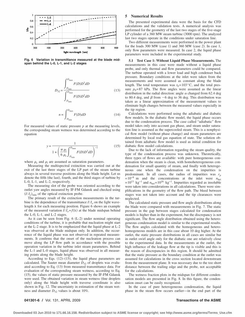
D32 =

�Dmin

Dmax

F�D�D3dD

�Dmin

Dmax

F�D�D2dD

�13�

n =�Dmin

Dmax

F�D�dD �14�

For measured values of static pressure p at the measuring levels,the corresponding steam wetness was determined according to theequation

y =1

1 + ��

6

�l

�v�

Dmin

Dmax

F�D�D3dD�−1 �15�

where �v and �l are assumed as saturation parameters.Measuring the multispectral extinction was carried out at the

exit of the last three stages of the LP part of the steam turbinealways in several traverse positions along the blade height. Let usdenote the fifth �the last�, fourth, and the third stages of turbine byL-0, L-1, and L-2, respectively.

The measuring slot of the probe was oriented according to theoutlet yaw angles measured by IF-FM Gdansk and checked using�I / Io�min of the optical extinction probe.

The primary result of the extinction measurements in the tur-bine is the dependence of the transmittance I / Io on the light wave-length � for each measuring position. Figure 6 shows an exampleof the measured variation I / Io= f�� at the blade midspan behindthe L-0, L-1, and L-2 stages.

As it can be seen from Fig. 6 �L-2� under nominal operatingconditions of the turbine, it is probable that nucleation might startat the L-2 stage. It is to be emphasized that the liquid phase at L-2was observed at the blade midspan only. In addition, the occur-rence of the liquid phase was not observed in repeated measure-ments. It confirms that the onset of the nucleation process canmove along the LP flow path in accordance with the possibleoperation variation in the turbine inlet steam parameters. Behindthe L-1 and L-0 stages, liquid phase was observed in all measur-ing points along the blade height.

According to Eqs. �12�–�15�, the liquid phase parameters arecalculated. The Sauter mean diameter D32 of droplets was evalu-ated according to Eq. �13� from measured transmittance data. Forevaluation of the corresponding steam wetness, according to Eq.�15�, the values of static pressure measured by the IF-FM Gdanskwere used. The obtained variation in steam wetness �fine dropletsonly� along the blade height with traverse coordinate is alsoshown in Fig. 12. The uncertainty in estimation of the steam wet-ness and diameter D32 values is about 10%.

5 Numerical ResultsThe presented experimental data were the basis for the CFD

calculations and the validation tests. A numerical analysis wasperformed for the geometry of the last two stages of the five-stageLP cylinder of a 360 MW steam turbine �3000 rpm�. The analyzedlast two stages operate in the conditions under saturation line.

Two different measurements were performed in the power plantfor the loads 300 MW �case 1� and 360 MW �case 2�. In case 1,only flow parameters were measured. In case 2, the liquid phaseparameters were included in the experimental study.

5.1 Test Case 1: Without Liquid Phase Measurements. Themeasurements in this case were made without a liquid phaseprobe, and only thermal and flow parameters could be compared.The turbine operated with a lower load and high condenser backpressure. Boundary conditions at the inlet were taken from themeasurements and were assumed as constant along the bladelength. The total temperature was t0=103°C, and the total pres-sure p0=87 kPa. The flow angles were assumed as the lineardistribution in the radial direction: angle � changed from 62.4 degto 80.4 deg, and � from �6 deg to 36 deg. This distribution wastaken as a linear approximation of the measurement values toeliminate high changes between the measured values especially inthe tip region.

Calculations were performed using the adiabatic and diabaticflow models. In the diabatic flow model, the liquid phase occursdue to the condensation process. The case called “adiabatic” flowmodel takes only into account gas phase, and steam under satura-tion line is assumed as the supercooled steam. This is a nonphysi-cal flow model �without phase change� and steam parameters aredetermined by local real gas equation of state. The solution ob-tained from adiabatic flow model is used as initial condition fordiabatic flow model calculations.

Due to the lack of information regarding the steam quality, thetype of the condensation process was unknown. Theoretically,three types of flows are available: with pure homogeneous con-densation when the steam is clean, with homoheterogeneous con-densation for small quantity of steam, and finally with heteroge-neous one when the condensation on the impurities ispredominant. In all cases, the radius of impurities was rp=10−8 m and the concentrations at the inlet were nhet=1013 kg−1 and nhet=1016 kg−1. Impurities regarded as insolublewere taken into considerations in all calculations. There were sim-plifications in the geometry of the flow path. The bleed betweenstages was not taken into account and the tip clearances wereneglected.

The calculated static pressure and flow angle distributions alongthe blade were compared with measurements in Fig. 7. The staticpressure in the gap between stages calculated for condensationmodels is higher than in the experiment, but the discrepancy is notsignificant. The flow angle distribution obtained using the hetero-geneous condensation model is similar to the experimental results.The flow angles calculated with the homogeneous and hetero-homogeneous models are in this case about 10 deg higher. At theoutlet, the static pressure distributions in all cases are similar butin outlet swirl angle only for the diabatic one are relatively closeto the experimental data. In the measurements at the outlet, thehigh influence of the leakage flow at the tip is visible and this isthe reason of discrepancies in this region. It should be admittedthat the static pressure as the boundary condition at the outlet wasassumed for calculations in the cross section located downstreamfrom the measurement plane. It was necessary due to the too shortdistance between the trailing edge and the probe, not acceptablefor the calculations.

The wetness fraction plots in the midspan for different conden-sation models are presented in Fig. 8. In this figure, the conden-sation onset can be easily recognized.

In the case of pure heterogeneous condensation, the liquidphase in the steam flow occurs earlier—in the end part of the

Fig. 6 Variation in transmittance measured at the blade mid-span behind the L-0, L-1, and L-2 stages



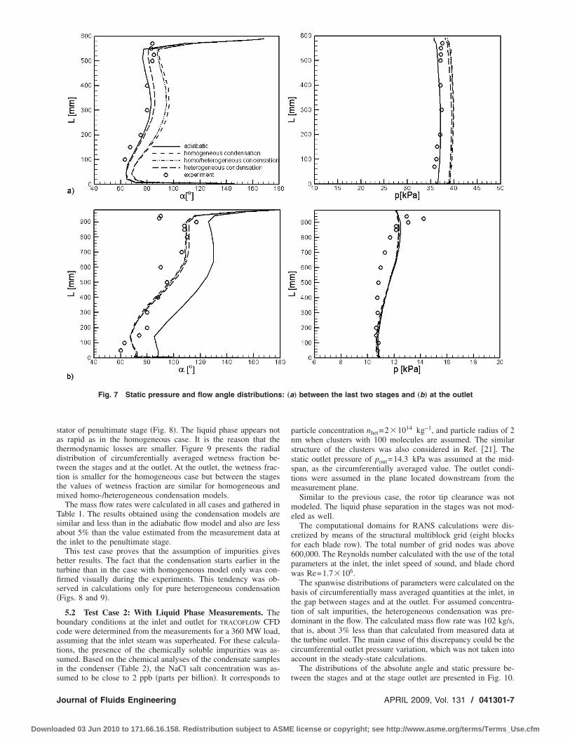
stator of penultimate stage �Fig. 8�. The liquid phase appears notas rapid as in the homogeneous case. It is the reason that thethermodynamic losses are smaller. Figure 9 presents the radialdistribution of circumferentially averaged wetness fraction be-tween the stages and at the outlet. At the outlet, the wetness frac-tion is smaller for the homogeneous case but between the stagesthe values of wetness fraction are similar for homogeneous andmixed homo-/heterogeneous condensation models.

The mass flow rates were calculated in all cases and gathered inTable 1. The results obtained using the condensation models aresimilar and less than in the adiabatic flow model and also are lessabout 5% than the value estimated from the measurement data atthe inlet to the penultimate stage.

This test case proves that the assumption of impurities givesbetter results. The fact that the condensation starts earlier in theturbine than in the case with homogeneous model only was con-firmed visually during the experiments. This tendency was ob-served in calculations only for pure heterogeneous condensation�Figs. 8 and 9�.

5.2 Test Case 2: With Liquid Phase Measurements. Theboundary conditions at the inlet and outlet for TRACOFLOW CFDcode were determined from the measurements for a 360 MW load,assuming that the inlet steam was superheated. For these calcula-tions, the presence of the chemically soluble impurities was as-sumed. Based on the chemical analyses of the condensate samplesin the condenser �Table 2�, the NaCl salt concentration was as-sumed to be close to 2 ppb �parts per billion�. It corresponds to

particle concentration nhet=2�1014 kg−1, and particle radius of 2nm when clusters with 100 molecules are assumed. The similarstructure of the clusters was also considered in Ref. �21�. Thestatic outlet pressure of pout=14.3 kPa was assumed at the mid-span, as the circumferentially averaged value. The outlet condi-tions were assumed in the plane located downstream from themeasurement plane.

Similar to the previous case, the rotor tip clearance was notmodeled. The liquid phase separation in the stages was not mod-eled as well.

The computational domains for RANS calculations were dis-cretized by means of the structural multiblock grid �eight blocksfor each blade row�. The total number of grid nodes was above600,000. The Reynolds number calculated with the use of the totalparameters at the inlet, the inlet speed of sound, and blade chordwas Re=1.7�106.

The spanwise distributions of parameters were calculated on thebasis of circumferentially mass averaged quantities at the inlet, inthe gap between stages and at the outlet. For assumed concentra-tion of salt impurities, the heterogeneous condensation was pre-dominant in the flow. The calculated mass flow rate was 102 kg/s,that is, about 3% less than that calculated from measured data atthe turbine outlet. The main cause of this discrepancy could be thecircumferential outlet pressure variation, which was not taken intoaccount in the steady-state calculations.

The distributions of the absolute angle and static pressure be-tween the stages and at the stage outlet are presented in Fig. 10.

Fig. 7 Static pressure and flow angle distributions: „a… between the last two stages and „b… at the outlet



The numerical results are compared with the experimental data.The calculated flow angles at the outlet coincide relatively well

with the measurement data �Fig. 10�b��. The comparison of cal-culated parameters with experiment between the stages is shownin Fig. 10�a�. The absolute outlet angle is within the range be-tween 60 deg and 90 deg without taking into account endwallboundary layers. The maximum discrepancy between the calcu-

lated and measured values is twice as big as the measurementerror. The calculated distribution of static pressure is consistentwith the experiment.

To show the wet steam formation, the blade-to-blade cross sec-tions of stages at the midspan are presented in Fig. 11. For theassumed soluble impurities in the steam, the condensation processshows homo- and heterogeneous patterns, but the second one is

Fig. 8 Wetness fraction at the midspan section: „a… homogeneous, „b… homoheteroge-neous, and „c… heterogeneous condensations

Fig. 9 Wetness fraction distributions: „a… between the last two stages and „b… at the outlet

Table 2 Results of chemical analyses of condensate samples

Notation pH Na+ K+ NH4+ Cl− SO4

− SiO2 Fe

Unit - �g /kg �g /kg �g /kg �g /kg �g /kg �g /kg �g /kgCondensate behind the LP part 8–8.4 2–3 5 - 2 1–2 2–3 7–8First condensate 6.8–6.9 180 40 60 130 90 900 1200



predominant. The liquid phase generated in the flow forms in65–70% on the salt particles. The beginning of the condensation

process is in the stator row of the first calculated stage �Fig.12�a��. The proper conditions for the homogeneous condensation

Fig. 10 Flow angle and static pressure distribution: „a… between the last two stages and „b… at the outlet

Fig. 11 Wetness fraction contours at midspan section: global wetness frac-tion contours „homogeneous and heterogeneous… „a… and wetness fractioncontours generated only due to the heterogeneous condensation „b…



are in the rotor row of the first stage as can be deduced from thewetness contours in Figs. 11�a� and 11�b�. The contours are shownfor the global wetness fraction obtained due to the homogeneousand heterogeneous condensation processes and for the wetnessfraction generated only on the soluble particles.

The spanwise distributions of the wetness fractions and dropletradii in the gap between stages and at the stage outlet are showntogether with experimental data in Fig. 12. The relatively goodagreement in the wetness fraction distributions is observed belowthe midsection at the outlet. The calculated wetness fraction be-tween the stages is about 30% smaller than that estimated fromthe experimental data. This difference is high in the midpart of theblade and decreases in the tip sections. The discrepancies at theoutlet are smaller than those between the stages. This can be ex-plained by fact that at the outlet the equilibrium in the wet steamwas achieved. The simplifications in condensation models and theaccuracy of the real-scale measurements bear on the discrepanciesin the flow parameters between the calculations and experiment.

In Fig. 12, the spanwise distributions of the Sauter mean diam-eters are presented. From calculations, the volume averaged diam-eter is obtained; therefore, the Sauter diameter was calculated onthe basis of droplet size spectrum known from experiment.

The calculated droplet radii show a more even distribution andare confined within the same range in the both sections.

6 Conclusions

The reported investigation of steam flow through the LP part ofa 360 MW turbine suggests that the heterogeneous condensationmight be a dominating process for the considered concentration ofimpurities �NaCl�. This could be the reason why supercooling isnot observed in the turbine, and the condensation starts practicallyclose to the saturation line. The optical extinction test reveals thatthe water droplets recorded in the turbine flow can be as large as300–500 nm in diameter. The comparison of the flow field param-eters obtained by means of TRACOFLOW in-house CFD code andfrom experimental data shows relatively good correspondence andconfirms proper modeling of the real gas properties and conden-sation processes in the steam flowing through the stages.

The applied CFD tool has been before thoroughly validatedagainst laboratory experiments. It has been possible to validate themathematical model under conditions present in the real turbine aswell.

It should be emphasized that it was the first step in the compre-hensive analysis of the condensation phenomena using numericaland experimental research made for the working steam turbine oflarge output.

Fig. 12 Wetness fraction and mean droplet Sauter diameter: „a… between the last two stages and „b… at the outlet



AcknowledgmentThe authors would like to thank the Polish Ministry of Science

and Information Technology for the financial support of the Re-search Project No. PB 1431/T10/2004/26 and the management ofthe Belchatow Power Plant for the consent for onsite measure-ments.

Nomenclatureaw � activity of water in solutionD � droplet diameter, m

D32 � Sauter mean droplet diameter, mE � Mie extinction functionF � distribution function of diameter D, m−3

h � specific enthalpy, J kg−1

Io � incident light intensity �no droplets�I � light intensityJ � nucleation rate, m−3 s−1

k � Boltzmann constant, J K−1

l � light path length in wet steam, mL � blade height, mm � relative refraction index, mass, kgm � mass flow rate, kg s−1

Ml � molality, mol kg−1

Mw � molal mass, kg kmol−1

n � number of droplets, kg−1

p � pressure, PaR � individual gas constant, J kg−1 K−1

r � radius, mr� � critical radius, ms � specific entropy, J kg−1 K−1

T � temperature, Ku ,v ,w � velocity components in Cartesian coordinates,

m s−1

y � wetness fraction, kg kg−1

Z � compressibility coefficientx ,y ,z � Cartesian coordinates, m

� � inclination angle, deg� � circumferential angle, deg� � wavelength of light, m, thermal conductivity,

W m−1 K−1

� � density, density of the mixture, kg m−3

� � isentropic exponent� � specific volume, m3 kg−1

� � surface tension, N m−1

Subscripts0 � total parameter

hom � homogeneoushet � heterogeneous

v � vapor phase

l � liquid phases � saturation value

w � water

References�1� Keller, H., 1974, “Erosionkorrosion an Nassdampfturbinen,” VGB Kraftwerk-

technik, 54, pp. 292–295.�2� Jonas, O., 1985, “Steam Turbine Corrosion,” Mat. Perf., 24�2�, pp. 9–18.�3� Bakhtar, F., White, A. J., and Mashmoushy, H., 2005, “Theoretical Treatments

of Two-Dimensional, Two-Phase Flows of Steam and Comparison With Cas-cade Measurements,” Proc. Inst. Mech. Eng., Part C: J. Mech. Eng. Sci., 219,pp. 1335–1355.

�4� Wróblewski, W., Dykas, S., and Gepert-Niedobecka, A., 2007, “CondensingSteam Flow Computations—Validation Problems,” Seventh European Confer-ence on Turbomachinery, Conference Proceedings, Athens, K. D. Papailiou, F.Martelli, and M. Manna, eds., pp. 841–848.

�5� Hesler, S., Shuster, L., and McCloskey, T., 1998, “Optical Probe of Measure-ment of Steam Wetness Friction in LP Turbine,” IPJC II, ASME, New York,PWR-Vol. 33.

�6� Bakhtar, F., and Heaton, A. V., 2005, “Effects of Wake Chopping on DropletSizes in Steam Turbines,” J. Mech. Eng. Sci., 219�C12�, pp. 1357–1367.

�7� Petr, V., Kolovratník, M., and Hanzal, V., 2003, “Instrumentation and Tests onDroplet Nucleation in LP Steam Turbines,” Power Plant Chemistry, 5�7�, pp.389–395.

�8� White, A. J., Young, J. B., and Walters, P. T., 1996, “Experimental Validationof Condensing Flow Theory for a Stationary Cascade of Steam TurbineBlade,” Philos. Trans. R. Soc. London, Ser. A, 354, pp. 59–88.

�9� Wagner, W., Cooper, J. R., Dittmann, A., Kijima, J., Kretzschmarr, H.-J.,Kruse, A., Mareš, R., Oguchi, K., Sato, H., Stöcker, I., Šifner, O., Takaishi, Y.,Tanishita, I., Trübenbach, J., and Willkommen, Th., 2000, “The IAPWS In-dustrial Formulation 1997 for the Thermodynamic Properties of Water andSteam,” Trans. ASME: J. Eng. Gas Turbines Power, 122�1�, pp. 150–181.

�10� Frenkel, J., 1946, Kinetic Theory of Liquids, Oxford University Press, NewYork.

�11� Gyarmathy, G., 1960, “Grundlagen einer Theorie der Nassdampfturbine,”Ph.D. thesis, ETH, Zürich.

�12� Kantrowitz, A., 1951, “Nucleation in Very Rapid Vapor Expansions,” J. Chem.Phys., 19, pp. 1097–1100.

�13� Gorbunov, B., and Hamilton, R., 1997, “Water Nucleation on Aerosol ParticlesContaining Both Soluble and Insoluble Substances,” J. Aerosol Sci., 28�2�, pp.239–248.

�14� Dykas, S., 2001, “Numerical Calculation of the Steam Condensing Flow,”Task Quarterly, Scientific Bulletin of Academic Computer Centre in Gdansk,5�4�, pp. 495–519.

�15� Wróblewski, W., Dykas, S., and Gepert, A., 2006, “Modeling of Steam FlowWith Heterogeneous Condensation,” Monografia 95, Wydawnictwo Politech-niki Sląskiej, Gliwice, in Polish.

�16� Lagun, V. P., Simoyu, L. L., and Frumin, Yu. Z., 1975, “Full-Scale Tests of theExhaust Hoods of a High-Capacity Steam Turbine,” Teploenergetika �Moscow,Russ. Fed.�, 22�2�, pp. 31–35.

�17� Gardzilewicz, A., and Marcinkowski, S., 1995, “Diagnosis of LP Steam Tur-bine Prospects of Measuring Techniques,” Proceedings of the ASME JointPower Generation Conference, Vol. 3, pp. 349–358.

�18� Gardzilewicz, A., Marcinkowski, S., Karwacki, J., and Kurant, B., 2006, “Re-sults of Measurements of Condensing Steam Flow in LP Part of Turbine 18 Kin Belchatow Power Plant,” IF-FM Report Nos. 5681 and 6157.

�19� Steltz, W., Lindsay, P., and Lee, W., 1983, “The Verification of ConcentratedImpurities in Low Pressure Steam Turbine,” ASME Winter Meeting, WA.

�20� Svododa, R., Phlug, H.-D., and Warnecke, T., 2003,“Investigation into theComposition of the Early Condensate in Steam Turbines,” Power Plant Chem-istry GmbH, Neulusshei.

�21� Petr, V., and Kolovratnik, M., 2001, “Heterogeneous Effects in the DropletNucleation Process in LP Steam Turbines,” Proceedings of the Fourth Euro-pean Conference on Turbomachinery, Florence, Italy, pp. 783–792.



M. Kawaji1

Department of Chemical Engineering and AppliedChemistry,

University of Toronto,200 College Street,

Toronto, ON, M5S 3E5, Canada

K. MoriDepartment of Mechanical Engineering,

Osaka Electro-Communication University,18-8 Hatsu-cho,

Neyagawa, Osaka, Japan 572-8530

D. BolintineanuDepartment of Chemical Engineering and Applied

Chemistry,University of Toronto,

200 College Street,Toronto, ON, M5S 3E5, Canada

The Effects of Inlet Geometry andGas-Liquid Mixing on Two-PhaseFlow in MicrochannelsThe effects of gas-liquid inlet geometry and mixing method on adiabatic gas-liquid two-phase flow in a microchannel of 100 �m diameter have been investigated using aT-junction inlet with the same internal diameter as the microchannel. Two-phase flowpatterns, void fraction, and friction pressure drop data obtained with the T-junction inletwere found to be significantly different from those obtained previously with a reducerinlet. For the T-junction inlet, the two-phase flow patterns in the microchannel werepredominantly intermittent flows with short gas and liquid plugs/slugs flowing with nearlyequal velocities. The void fraction data then conformed nearly to that of a homogeneousflow model, and the two-phase friction multiplier data could be described by theLockhart–Martinelli correlation applicable to larger channels. However, when a reducerinlet was used previously and the diameter of the inlet section was much larger than thatof the microchannel, an intermittent flow of long gas slugs separated by long liquid slugsbecame prevalent and the void fraction decreased to values far below the homogeneousvoid fraction. The differences in the two-phase flow characteristics between a T-junctioninlet and reducer inlet were attributed to the differences in the gas bubble/slug generationmechanisms. �DOI: 10.1115/1.3089543�

1 IntroductionFew two-phase flow studies are yet available in the literature

that involved a microchannel diameter of 100 �m or less as notedin recent reviews by Serizawa �1� and Thome �2�. The availableresults for microchannels have shown certain differences fromthose for conventional channels: bubbly and droplet flows maynot always occur in microchannels, the void fraction data in mi-crochannels may deviate from the Armand correlation �3� and thetwo-phase friction pressure drop in microchannels could be pre-dicted by conventional models.

The available results also indicate that the adiabatic two-phaseflow characteristics in the same microchannel such as flow pat-terns, void fraction, and friction pressure drop can vary signifi-cantly depending on the microchannel inlet configuration and thegas-liquid mixing method, unlike in minichannels and conven-tional channels.

Stanley et al. �4� investigated two-phase pressure drop and heattransfer in the square and rectangular aluminum channels of hy-draulic diameters Dh ranging from 56 �m to 256 �m. Theymixed water with argon, helium, or nitrogen gas upstream of themicrochannel and injected the two-phase mixture from a 1

4 in.tube into the microchannel test section, so the inlet was a reducerwith sudden reduction in diameter from 1

4 in. to 56–256 �m.They reported that the conventional semi-empirical correlationsfor two-phase pressure drop overpredicted their microchannel datasubstantially.

Air-water two-phase flow experiments were conducted in25 �m and 100 �m circular microchannels connected to areducer-type inlet by Serizawa and co-workers �5,6�. Five flowpatterns were observed: dispersed bubbly flow, gas slug flow,liquid-ring flow, liquid lump flow, and liquid droplet flow. Theoccurrence of liquid-ring flow and liquid lump flow clearly indi-

cated that there are differences in the flow patterns between mi-crochannels of D�100 �m and minichannels of D�1 mm.

Kawaji and co-workers �7,8� investigated the two-phase flow ofnitrogen gas and water through horizontal circular microchannelsof 50–250 �m diameter. The gas and liquid were mixed in areducer inlet where the diameter changed from 750 �m down tothe microchannel diameter. They reported significant differencesin the flow pattern maps and void fraction data from those previ-ously described for minichannels with diameters above �1 mm.In particular, they reported the existence of flow patterns unique tomicrochannels �liquid-ring flow and serpentinelike gas core flow�.Furthermore, the time-average void fraction data deviated fromArmand’s correlation �3�, which is normally applicable to min-ichannels with diameters �1 mm. This was in contrast with thevoid fraction data of Serizawa et al. �6� for a 20 �m circularmicrochannel, which could be well described by Armand’s typecorrelation.

Chung et al. �9� later found that the two-phase flow character-istics in a 96 �m square channel and a 100 �m circular channelconnected to the same reducer inlet used by Kawahara et al. �7�were quite similar and independent of the channel cross sectionfor a mixture of nitrogen gas and water. Furthermore, Kawahara etal. �10� found only a moderate effect of fluid properties such asliquid viscosity and surface tension on the two-phase flow char-acteristics in a microchannel.

Besides the reducer-type inlet, several different inlet designsand gas-liquid mixing methods have been used to inject a two-phase mixture into a microchannel. A simple T-junction has alsobeen popular particularly for microfluidic applications as used byThorsen et al. �11�, Okushima et al. �12�, Günther et al. �13�, Xu etal. �14�, Garstecki et al. �15�, and Ide et al. �16�, among others. Inmany cases, the T-junction diameter was the same as or close tothe microchannel diameter, and its use was intended to producemonodisperse microbubbles. On the other hand, a much larger�1/8 in.� diameter T-junction was used by Xiong and Chung �17�upstream of a rectangular microchannel. The gas was injected intothe liquid stream through a 200 �m diameter needle, which wasinserted from the branch of the T-junction so that the needle tipwould be positioned in the middle of the T-junction.


JOURNAL OF FLUIDS ENGINEERING. Manuscript received October 8, 2007, final manu-script received January 19, 2009; published online March 11, 2009. Assoc. Editor:Theodore Heindel. Paper presented at the Third International Conference on Micro-channels and Minichannels �ICMM2005�, Toronto, ON, Canada, June 13–15, 2005.



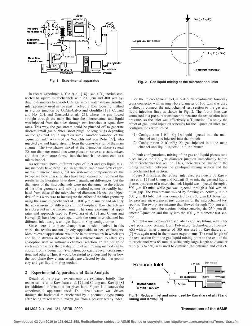
In recent experiments, Yue et al. �18� used a Y-junction con-nected to square microchannels with 200 �m and 400 �m hy-draulic diameters to absorb CO2 gas into a water stream. Anotherinlet geometry used in the past involved a flow focusing methodin a cross junction by Gañán-Calvo and Gordillo �19�, Cubaudand Ho �20�, and Garstecki et al. �21�, where the gas flowedstraight through the main line into the microchannel and liquidwas injected from the sides through two branches at equal flowrates. This way, the gas stream could be pinched off to generatediscrete small gas bubbles, short plugs, or long slugs dependingon the gas and liquid injection rates. Another variation of theT-junction inlet was used by Waelchli and von Rohr �22�, whoinjected gas and liquid streams from the opposite ends of the mainchannel. The two phases mixed at the T-junction where several50 �m diameter round pins were placed to serve as a static mixer,and then the mixture flowed into the branch line connected to amicrochannel.

As reviewed above, different types of inlet and gas-liquid mix-ing methods have been used in adiabatic two-phase flow experi-ments in microchannels, but no systematic comparisons of thetwo-phase flow characteristics have been carried out. Some of theresults in the literature have shown significant differences, but thediameters of the microchannels were not the same, so the effectsof the inlet geometry and mixing method cannot be readily iso-lated from those of the microchannel diameter. Hence, the objec-tive of this work was to investigate the effect of the inlet geometryusing the same microchannel of �100 �m diameter and identifythe key reasons for differences in the two-phase flow characteris-tics observed in the microchannel. The same experimental appa-ratus and approach used by Kawahara et al. �7� and Chung andKawaji �8� have been used again with the same microchannel butdifferent inlet designs and gas-liquid mixing configurations.

Since there is no phase change heat transfer involved in thiswork, the results are not directly applicable to heat exchangers.Most relevant applications would be in microreactors in which gasand liquid streams are contacted in a microchannel to effect gasabsorption with or without a chemical reaction. In the design ofsuch microreactors, the gas-liquid inlet and mixing method can bechosen from a T-junction, Y-junction, co-axial reducer, cross junc-tion, and others. Thus, it would be useful to understand better howthe two-phase flow characteristics are affected by the inlet geom-etry and gas-liquid mixing method.

2 Experimental Apparatus and Data AnalysisDetails of the present experiments are explained briefly. The

reader can refer to Kawahara et al. �7� and Chung and Kawaji �8�for additional information not given here. Figure 1 illustrates theexperimental apparatus used. De-ionized water was driventhrough the horizontal microchannel by a pneumatic-type pumpafter being mixed with nitrogen gas from a pressurized cylinder.

For the microchannel inlet, a Valco Nanovolume® four-waycross connector with an inner bore diameter of 100 �m was usedto directly connect the microchannel test section to the gas andliquid injection lines as shown in Fig. 2. The fourth line wasconnected to a pressure transducer to measure the test section inletpressure, so the inlet was effectively a T-junction. To study theeffect of gas-liquid injection schemes for the T-junction inlet, twoconfigurations were tested.

�1� Configuration 1 �ConFig 1�: liquid injected into the mainchannel and gas injected into the branch

�2� Configuration 2 �ConFig 2�: gas injected into the mainchannel and liquid injected into the branch.

In both configurations, mixing of the gas and liquid phases tookplace inside the 100 �m diameter junction immediately beforethe microchannel test section. Thus, there was no change in thetubing diameter between the gas-liquid mixing section and themicrochannel test section.

Figure 3 illustrates the reducer inlet used previously by Kawa-hara et al. �7� and Chung and Kawaji �8� to mix the gas and liquidphases upstream of a microchannel. Liquid was injected through a500 �m ID tube, while gas was injected through a 200 �m an-nular gap. The two streams mixed by flowing collectively into a500 �m ID tube that was connected to a 250 �m ID T-junctionfor pressure measurement just upstream of the microchannel testsection. The two-phase mixture thus flowed through 750 �m and500 �m diameter tube sections before entering the 250 �m di-ameter T-junction and finally into the 100 �m diameter test sec-tion.

A circular microchannel �fused silica capillary tubing with stan-dard polyimide coating from Polymicro Technologies, Phoenix,AZ� with an inner diameter of 100 �m used by Kawahara et al.�7� was again used in the present experiments. The total length ofthe test section from the gas-liquid mixing point to the exit of themicrochannel was 65 mm. A sufficiently large length-to-diameterratio �L /D=650� was used to diminish the entrance and exit ef-

Fig. 1 Experimental apparatus Fig. 2 Gas-liquid mixing at the microchannel inlet

Fig. 3 Reducer inlet and mixer used by Kawahara et al. †7‡ andChung and Kawaji †8‡



fects. The window for flow visualization was located as far backas possible �46.1 mm from the gas-liquid mixing point� on themicrochannel to achieve a well-developed flow.

Three pressure transducers �PX303 series from Omega Engi-neering �Stamford, CT�� covering different ranges�3450�8.6 kPa, 690�1.7 kPa, and 210�0.52 kPa� were usedto measure the pressure drop between the microchannel inlet andoutlet. The liquid was discharged freely from the test section, sothat the pressure was atmospheric and temperature ambient at themicrochannel outlet.

The liquid flow rate was determined by using a load cell�50.97�0.255 g, model ELJ-0.5N from Entran Devices �Fair-field, NJ�� to weigh the discharged liquid collected over time. Thegas flow rate was measured using three mass flow meters �model179A-23012 from MKS Instruments �Andover, MA�, and models8172-0411 and 8172-0451 from Matheson Gas Products �Mont-gomeryville, PA�� to encompass a wide range of conditions�1�0.01 sccm, 10�0.1 sccm, and 50�0.5 sccm�. The analogsignals for all of the pressure, temperature, and mass flow ratereadings were sampled at 10 Hz by a 16-bit data acquisition sys-tem �model NI 6035E from National Instruments �Austin, TX��.

Background illumination to see the flow patterns was generatedby a cold lamp �model DCR III from Schott-Fostec �Auburn,NY�� located behind the test section. The view field was magni-fied by attaching a 20� microscope objective lens �model 378-802-2 from Mitsutoyo America Corporation �Aurora, IL�� to thevideo camera. A monochrome CCD camera �model TM-1040from Pulnix America �Sunnyvale, CA�� with a resolution of1024�H��1024�V� pixels, a maximum frame rate of 30 fps, anda shutter speed of 1/16,000 s was used for image capturing. Theproblem of optical distortion was dealt with earlier by Kawaharaet al. �7�. They elected to not correct for optical distortion so thatthe images of the gas-liquid interfacial structure near the channelwall could be enlarged and better examined. Likewise, opticaldistortion is not addressed here for the same reason.

The previous experiments covered a range of 0.01� jL�5.77 m /s for the superficial liquid velocity and 0.02� jG,avg�73 m /s for the average superficial gas velocity. The new ex-periments covered slightly smaller ranges: 0.027� jL�2.05 m /sand 0.1� jG,avg�50 m /s. The values of dimensionless param-eters calculated for the previous experiments are the Bond number�0.000083�Bo�0.0095�, the superficial Weber number for liq-uid �0.00057�WeLS�116� and gas �0.0000020�WeGS�12�,the superficial Reynolds number for liquid �2�ReLS�2300� andgas �0.4�ReGS�751�, and the capillary number �0.00013�CaL

�0.070�. These values indicate the relative magnitudes of theforces involved �inertia�surface tension�viscous force�gravity�.

2.1 Measurement Uncertainties and Data Analyses. Themeasurement uncertainties estimated for the present experimentsare summarized in Table 1. A propagation of error analysis �23�was performed to estimate the uncertainties in the derived quan-tities such as superficial velocities, void fraction, and pressuregradients.

Initially, experiments were conducted with de-ionized water tocalculate the single-phase friction factor from the frictional pres-sure drop. The computed friction factor was compared with theconventional value for laminar flow in a pipe. The two-phase fric-tional pressure drop was calculated by subtracting estimates of thepressure drop due to inlet contraction and flow acceleration fromthe total pressure drop measured in the horizontal channel. Toestimate the pressure drop attributed to the acceleration of theflow, the void fraction at the inlet and outlet of the test section wasestimated based on the homogeneous flow model.

3 Results and DiscussionThe experimental results on the two-phase flow patterns, void

fraction, and two-phase friction pressure drop obtained with aT-junction inlet will be presented and compared with those re-ported previously by Kawahara et al. �7� for a reducer inlet todetermine the effects of inlet geometry and gas-liquid mixingmethod.

3.1 Two-Phase Flow Patterns. The two-phase flow patternsobtained in the present experiments are found to be quite differentfrom those observed in our previous work. Typical examples ofthe flow patterns seen in the present experiments for both Con-figurations 1 and 2 are shown in Fig. 4. Short gas bubbles or plugssuch as those shown in Figs. 4�a� and 4�b� were seldom observedin the previous experiments using a series of reducer sectionsbetween the gas-liquid mixer and the microchannel test section.Instead, slug flows with a long gas core shown in Fig. 4�c� andsurrounded by a thin, thick, or wavy liquid film were predomi-nant. Thus, the flow patterns observed in the present experimentswere classified differently from the previous experiments and ac-cording to the following definitions.

�1� Bubbly flow: the presence of spherical bubbles whose di-ameters are less than the diameter of the microchannel

�2� Plug flow: the presence of gas plugs that are shorter thanthe width of the viewing window ��250 �m� and areseparated by liquid bridges

Table 1 Measurement uncertainties

Parameters Uncertainty range

Mass flow rate of liquid, mL �0.1% to �1%Mass flow rate of gas, mG �1% to �10%Superficial liquid velocity, jL �2.1% to �3%Superficial gas velocity, jG �3% to �12%Void fraction, � � 0.05Total two-phase pressure gradient, ��P /�Z� �1% to �4%Two-phase frictional pressure gradient, ��Pf /�Z�TP �2% to �7%Two-phase friction multiplier, L

2 �2% to �7%

Fig. 4 Two-phase flow patterns observed in a microchannelwith a micro-T-junction inlet



�3� Slug flow: the presence of gas slugs that are longer than theviewing window

�4� Semi-annular flow: long gas core surrounded by a liquidfilm and interrupted by infrequent liquid slugs

�5� Ring flow: 10% or more of the images for a given run havea ring-shaped liquid film surrounding the gas core

The two-phase flow pattern maps were then constructed basedon the above definitions for the two T-junction inlet configurationsas shown in Fig. 5. At low superficial gas velocities jG1 m /s,bubbly flow, plug flow, and slug flow patterns appeared at pro-gressively lower liquid flow rates. At moderate to high superficialgas velocities jG�2 m /s, slug and semi-annular flow patternswere observed. An open circle �� in Figs. 5�a� and 5�b� indicatesthe occasional appearance of a ring-film flow pattern.

The difference in the gas and liquid injection configurations forthe micro-T-junction inlet had only a small effect on the flowpattern map as clear from a comparison of Fig. 5�a� and 5�b�.However, these results for the micro-T-junction inlet were signifi-cantly different from the map previously obtained for a reducerinlet case by Kawahara et al. �7� and shown in Fig. 5�c�. When theinlet section consisted of a series of reducer sections from750 �m to 100 �m �Fig. 2�, the predominant flow pattern ob-

served was a slug flow with a long gas core surrounded by a thin,thick or ring-shaped film. Depending on the frequency of the ap-pearance of different liquid film shapes, the flow patterns weredefined as slug-ring, ring-slug, and multiple flows �Fig. 5�c��.

Although a semi-annular flow pattern was observed in bothmicro-T-junction and reducer inlet experiments, a strong differ-ence existed between them in the appearance of short gas bubblesand plugs. This is due to the fact that small gas bubbles are readilycreated at the T-junction inlet as reported in previous studies. Themechanism of small gas bubble generation at the micro-T-junctioncan be readily illustrated as shown in Fig. 6. Such a mechanismhad been previously investigated for the ConFig. 1 case �liquidinjected into the main channel while gas is injected into thebranch, Fig. 6�a�� by Shibata et al. �24�. Short gas plugs wereobserved to be generated as a result of interfacial instability orpinch-off at the corner of the T-junction as shown in Figs.6�b�–6�e�.

Although no flow visualization was conducted for ConFig. 2, asimilar interfacial instability or pinching off of a gas bubble orplug at the micro-T-junction can be conjectured. Thus, regardlessof which phase is injected into the main channel or the branch, theuse of a T-junction to mix and inject the gas-liquid mixture into amicrochannel can result in two-phase flow patterns that are verydifferent from those observed in the reducer inlet case. The largerinlet cross section �D=750 �m� for the reducer inlet used byKawahara et al. �7� would allow larger gas bubbles to form up-stream of the microchannel test section. When these gas bubblesflow into the microchannel with a much smaller diameter �D=100 �m�, the gas slug length would increase by more than 50times, as illustrated in Fig. 7. Thus, for example, if the diameter ofthe gas bubble formed in the inlet section were 2 mm, then itwould form a 100 mm long gas slug in the microchannel. This canexplain why Kawahara et al. �7� obtained mostly long gas coreflows with a reducer inlet rather than short gas plug flows.

The present flow pattern results obtained with a T-junction inletare now compared with the previous results obtained with othertypes of inlet as shown in Fig. 8. Only the bubbly-to-plug �or slug�and slug-to-annular �or semi-annular� flow pattern transitionboundaries are indicated. Although the transition boundaries arerepresented by thin lines, the flow patterns did not change assharply as suggested by those lines. Nevertheless, the present

Fig. 5 Two-phase flow pattern maps for a micro-T-junction in-let „a… ConFig. 1 and „b… ConFig. 2, and „c… a reducer inlet usedby Kawahara et al. †7‡ „an open circle indicates the occasionalappearance of a ring-film flow pattern…

Fig. 6 Sequence of images showing gas plug generation at amicro-T-junction „from Ref. †24‡…



T-junction inlet results are in general agreement with previousstudies for both bubbly-to-slug and slug-to-annular flow transitionboundaries.

It is noted in Fig. 8 that unlike the reducer inlet results obtainedby Kawahara et al. �7�, the flow pattern transition boundaries ob-tained by Serizawa et al. �6� are in agreement with the T-junctioninlet results. This may be attributed to the small diameter of thegas injection nozzle �D=40 �m� used within the 300 �m diam-eter reducer inlet section, which was connected to a 25 �m di-ameter microchannel. The size of the gas bubbles generated couldhave been much smaller than the internal diameter of the reducerdue to the small size of the gas injection nozzle and the effect ofco-axially flowing liquid, so the phenomenon illustrated in Fig. 7may not have occurred in the experiments of Serizawa et al. �6�.

3.2 Void Fraction. The differences in the two-phase flow pat-terns obtained in microchannels with a T-junction inlet and re-ducer inlet can also cause large differences in the void fraction asdiscussed below. To estimate the void fraction in the 100 �mmicrochannel, about 300 video images were analyzed for eachrun. The instantaneous void fraction was estimated for plug flowimages such as those shown in Fig. 4 by measuring the length ofa gas bubble or plug and calculating the volume by assuming acylindrical shape with semispherical caps. The instantaneous voidfraction was then computed as the ratio of the gas volume to thetotal channel volume within the viewing window. The imageswere assigned a void fraction of zero when they showed only theliquid flowing alone in the entire view window or a void fractionof unity when they showed a continuous gas core with a thin-smooth liquid film or ring-shaped liquid film. The time-averagedvoid fraction was then obtained by averaging the instantaneous

void fraction values from about 300 images. The effect of opticaldistortion on the above-mentioned method of measuring the voidfraction, particularly for long gas core flows with ring-shapedfilms and thick liquid films, was previously addressed by Kawa-hara et al. �7�.

The time-averaged void fraction �� data for the T-junction inletare plotted against the volumetric quality ��=�JG /JG+JL�� in Figs.9 and 10 for Configurations 1 and 2, respectively. The homoge-neous flow model ��=�� and the Armand correlation �3� for nar-row channels recommended by Ali et al. �25� are also shown inthe figures, respectively. Ali et al. �25� recommended using a cor-relation of the form ��=0.8�� originally developed by Armand �3�for narrow rectangular channels with DH�1 mm.

Both Configurations 1 and 2 data show a linear relationshipbetween the void fraction and volumetric quality, consistent withthe homogeneous flow model and Armand’s correlation, but un-like the nonlinear relationship obtained by Kawahara et al. �7� forthe reducer inlet case and given by

� =0.03�0.5

1 − 0.97�0.5 �1�

Equation �1� indicates the void fraction to increase slowly withincreasing volumetric quality and then exponentially after ��0.8. This trend implies a strong departure from homogeneousflow and indicates a large velocity slip between the liquid and gasphases.

Thus, as the inlet geometry was changed from a reducer toT-junction, the two-phase flow patterns in the microchannelchanged and this also strongly affected the time-average void frac-tion. For example, a plug flow pattern with alternating passages of

Fig. 7 Formation of a long gas slug from a bubble in a reducer inlet „not to scale…

Fig. 8 Comparison of flow pattern transition boundaries



short gas and liquid plugs as shown in Fig. 4 would lead to a slipratio close to unity, which is representative of a homogeneousflow. Since such a plug flow pattern was not observed in thereducer inlet case, the void fraction deviated strongly from thehomogeneous flow model in the experiments of Kawahara et al.�7�. The present data show that the inlet geometry and the methodof gas-liquid mixing can drastically change the time-average voidfraction for the same microchannel at given superficial gas andliquid velocities.

3.3 Friction Pressure Drop. The two-phase friction pressuredrop was evaluated from the measured total pressure drop by sub-tracting the acceleration pressure drop. The data were correlatedusing the Lockhart–Martinelli correlation �26�, which was devel-oped based on a separated flow assumption. This correlation usesa two-phase friction multiplier L

2 defined as follows:

��Pf

�Z�

TP= L

2��Pf

�Z�

L

�2�

where ��Pf /�Z�L is the frictional pressure drop when liquid isassumed to flow alone in the channel.

The two-phase friction multiplier has been correlated in termsof the Lockhart–Martinelli parameter X given by

X2 =��Pf/�Z�L

��Pf/�Z�G�3�

where ��Pf /�Z�G is the frictional pressure drop when the gas isassumed to flow alone in the channel. A widely used correlation tocalculate the friction multiplier is that proposed by Chisholm andLaird �27�.

L2 = 1 +

C

X+

1

X2 �4�

where the coefficient C is a constant ranging in value from 5 to 20for larger channels, depending on whether the liquid and gas flowsare laminar or turbulent. In conventional channels and minichan-nels, a strong mass velocity effect has been observed in the two-phase friction multiplier data �25�, because the flow can changefrom laminar to turbulent as the total mass velocity is increased.The C-value in Eq. �4� is also known to decrease as the channel’shydraulic diameter is reduced �28,29�.

The two-phase friction multiplier data obtained with aT-junction inlet in the present experiments are compared with theLockhart–Martinelli correlation in Fig. 11. Also shown are thecurves given by Eq. �4� with C=5 and the best fit values of C=2.0 and 2.5 for the present experiments, as well as C=0.24 forthe reducer inlet experiments obtained by Kawahara et al. �7�.Overall, the Lockhart–Martinelli model with properly chosen val-ues of C can be used to predict the two-phase friction multiplierdata reasonably well for the T-junction inlet experiments. Switch-ing the gas and liquid injection lines in the T-junction �Configu-rations 1 and 2� is seen to have only a minor effect.

The data from the T-junction inlet experiments for both Con-figurations 1 and 2 can be represented by different C-value curvesdepending on the range of the Lockhart–Martinelli parameter �C=2.0 or 2.5 for X2, and C=5 for X�3�. These C-values aremore than ten times greater than the value of C�=0.24�, obtainedfor the reducer inlet by Kawahara et al. �7�. Although not shownhere, only small deviations from the C=0.24 curve were seen forthe reducer inlet data for comparable ranges of gas and liquid flowrates tested �7�. This is likely to be due to a greater variety of flowpatterns observed in the T-junction inlet experiments describedearlier. Thus, as in the void fraction data, the two-phase friction

Fig. 9 Void fraction data for Configuration 1 of the T-junctioninlet; „– – –… homogeneous model „ε=�…, „——… Armand corre-lation „ε=0.833�…, and „----… Eq. „1……

Fig. 10 Void fraction data for Configuration 2 of the T-junctioninlet; „– – –… homogeneous model „ε=�…, „——… Armand corre-lation „ε=0.833�…, „----… „Eq. „1……

Fig. 11 Two-phase friction multiplier data for „a… ConFig. 1 and„b… ConFig. 2 of the T-Junction Inlet



pressure drop could be significantly different between theT-junction and the reducer inlet cases indicating the strong effectof the inlet geometry.

4 ConclusionThe effects of inlet geometry and gas-liquid injection method

on adiabatic two-phase flow in a 100 �m microchannel havebeen investigated experimentally. Nitrogen gas and water wereinjected into a micro-T-junction with the same diameter as themicrochannel connected downstream. The two-phase flow pat-terns observed have been found to differ strongly from those ob-tained in a previous study using a reducer inlet and a 750 �mdiameter mixing section. For the micro-T-junction inlet, plug andslug flows with alternating short gas plugs and liquid slugs wereobserved, which were rarely observed in the reducer inlet case.

Due to the obvious differences in the flow patterns observed,the void fraction data for the micro-T-junction inlet case agreedwith the homogeneous flow model, unlike the data obtained witha reducer inlet with a 750 �m diameter mixing section. The two-phase friction multiplier data could be well correlated in terms ofthe Lockhart–Martinelli parameter but the value of the constant Cin Chisholm’s correlation was much larger than the value obtainedfor the reducer inlet case.

Since the time-average void fraction �and consequently interfa-cial area� and friction pressure drop would strongly affect theperformance of microchannel devices such as microreactors fordirect contacting of gas and liquid streams, the dimensions andtype of a gas-liquid mixer to be used at the microchannel inletwould have to be carefully considered in the design process.

AcknowledgmentThis work was supported by a Discovery research grant from

the Natural Sciences and Engineering Research Council ofCanada. K. Mori would like to thank Osaka Electro-Communication University for a research leave grant, which al-lowed a one-year stay at the University of Toronto.

NomenclatureBo � Bond numberC � coefficient in Eq. �4�

Ca � capillary numberD � tube inner diameter �m�g � gravitational acceleration �m /s2�j � superficial velocity �m/s�

L � length �m�m � mass flow rate �kg/s�P � pressure �Pa�

Re � Reynolds numberu � axial velocity �m/s�

We � Weber numberX � Lockhart–Martinelli parameterZ � flow direction coordinate �m�

Greek Symbols� � volumetric quality� � void fraction

�P � pressure drop� � dynamic viscosity �Pa s�

L2 � two-phase friction multiplier � density �kg /m3�� surface tension �N/m�

Subscriptsf � friction

G � gas phaseL � liquid phase

M � mixing section

S � superficialTP � two-phase

References�1� Serizawa, A., 2006, “Gas-Liquid Two-phase Flow in Microchannels,” Multi-

phase Flow Handbook, C. T. Crowe, ed., CRC Press, Boca Raton, FL.�2� Thome, J. R., 2006, “State-of-the-Art Overview of Boiling and Two-Phase

Flows in Microchannels,” Heat Transfer Eng., 27�9�, pp. 4–19.�3� Armand, A. A., 1946, “The Resistance during the Movement of a Two-phase

System in Horizontal Pipes,” Izv. Vses. Teplotekh. Inst. �AERE-Lib/Trans.828�, 1, pp. 16–23.

�4� Stanley, R. S., Barron, R. F., and Ameel, T. A., 1997, “Two-Phase Flow inMicrochannels,” Micro-Electro-Mechanical Systems (MEMS), ASME, DSC-Vol. 62/HTD-Vol. 354, New York, pp. 143–152.

�5� Serizawa, A., and Feng, Z. P., 2001, “Two-Phase Flow in Micro-Channels,”Proceedings of the Fourth International Conference on Multiphase Flow, NewOrleans, LA, May 27–Jun. 1.

�6� Serizawa, A., Feng, Z., and Kawara, Z., 2002, “Two-Phase Flow in Micro-channels,” Exp. Therm. Fluid Sci., 26�6–7�, pp. 703–714.

�7� Kawahara, A., Chung, P. M.-Y., and Kawaji, M., 2002, “Investigation of Two-Phase Flow Pattern, Void Fraction and Pressure Drop in a Microchannel,” Int.J. Multiphase Flow, 28�9�, pp. 1411–1435.

�8� Chung, P. M. Y., and Kawaji, M., 2004, “The Effect of Channel Diameter onAdiabatic Two-Phase Flow Characteristics in Microchannels,” Int. J. Multi-phase Flow, 30�7–8�, pp. 735–761.

�9� Chung, P. M.-Y., Kawaji, M., Kawahara, A., and Shibata, Y., 2004, “Two-Phase Flow Through Square and Circular Microchannels—Effect of ChannelGeometry,” ASME J. Fluids Eng., 126�4�, pp. 546–552.

�10� Kawahara, A., Kawaji, M., Chung, P. M.-Y., Sadatomi, M., and Okayama, K.,2005, “Effects of Channel Diameter and Liquid Property on Void Fraction inAdiabatic Two-Phase Flow Through Microchannels,” Heat Transfer Eng.,26�3�, pp. 13–19.

�11� Thorsen, T., Roberts, R. W., Arnold, F. H., and Quake, S. R., 2001, “DynamicPattern Formation in a Vesicle-Generating Microfluidic Device,” Phys. Rev.Lett., 86, pp. 4163–4166.

�12� Okushima, S., Nishisako, T., Torii, T., and Higuchi, T., 2004, “ControlledProduction of Monodisperse Double Emulsions by Two-Step Droplet Breakupin Microfluidic Devices,” Langmuir, 20, pp. 9905–9908.

�13� Günther, A., Khan, S. A., Thalmann, M., Trachsel, F., and Jensen, K. F., 2004,“Transport and Reaction in Microscale Segmented Gas—Liquid Flow,” LabChip, 4, pp. 278–286.

�14� Xu, J. H., Li, S. W., Wang, Y. J., and Luo, G. S., 2006, “Controllable Gas-Liquid Two Phase Flow Patterns and Monodispersive Microbubbles in a Mi-crofluidic T-Junction Device,” Appl. Phys. Lett., 88, pp. 133506.

�15� Garstecki, P., Fuerstman, M. J., Stone, H. A., and Whitesides, G. M., 2006,“Formation of Droplets and Bubbles in a Microfluidic T-Junction—Scalingand Mechanism of Break-Up,” Lab Chip, 6, pp. 437–446.

�16� Ide, H., Kimura, R., and Kawaji, M., 2007, “Optical Measurement of VoidFraction and Bubble Size Distributions in a Microchannel,” Heat TransferEng., 28�8�, pp. 713–719.

�17� Xiong, R., and Chung, J. N., 2007, “An Experimental Study of the Size Effecton Adiabatic Gas-Liquid Two-phase Flow Patterns and Void Fraction in Mi-crochannels,” Phys. Fluids, 19, p. 033301.

�18� Yue, J., Chen, G. W., and Yuan, Q., 2004, “Pressure Drops of Single andTwo-Phase Flows Through T-Type Microchannel Mixers,” Chem. Eng. J.,102, pp. 11–24.

�19� Gañán-Calvo, A. M., and Gordillo, J. M., 2001, “Perfectly Monodisperse Mi-crobubbling by Capillary Flow Focusing,” Phys. Rev. Lett., 87, p. 274501.

�20� Cubaud, T., and Ho, C. M., 2004, “Transport of Bubbles in Square Microchan-nels,” Phys. Fluids, 16, pp. 4575–4585.

�21� Garstecki, P., Stone, H. A., and Whitesides, G. M., 2005, “Mechanism forFlow-Rate Controlled Breakup in Confined Geometries: A Route to Monodis-perse Emulsions,” Phys. Rev. Lett., 94, p. 164501.

�22� Waelchli, S., and von Rohr, P. R., 2006, “Two-Phase Flow Characteristics inGas—Liquid Microreactors,” Int. J. Multiph. Flow, 32�7�, pp. 791–806.

�23� Kline, S. J., and McClintock, F. A., 1953, “Describing Uncertainties in SingleSample Experiments,” Mech. Eng. �Am. Soc. Mech. Eng.�, 75, pp. 3–8.

�24� Shibata, Y., Ikeda, K., Hanri, T., Chung, P. M. Y., and Kawaji, M., 2003,“Study on Two-Phase Flow Through a T-Junction,” Proceedings of the FourthASME-JSME Joint Fluids Engineering Conference, Honolulu, Hawaii, Jul.6–11, Paper No. FDSM2003-45385.

�25� Ali, M. I., Sadatomi, M., and Kawaji, M., 1993, “Two-Phase Flow in NarrowChannels Between Two Flat Plates,” Can. J. Chem. Eng., 71�5�, pp. 657–666.

�26� Lockhart, R. W., and Martinelli, R. C., 1949, “Proposed Correlation of Datafor Isothermal Two-Phase, Two-Component Flow in Pipes,” Chem. Eng. Prog.,45�1�, pp. 39–48.

�27� Chisholm, D., and Laird, A. D. K., 1958, “Two-Phase Flow in Rough Tubes,”Trans. ASME, 80�2�, pp. 276–286.

�28� Mishima, K., and Hibiki, T., 1996, “Some Characteristics of Air-Water Two-Phase Flow in Small Diameter Vertical Tubes,” Int. J. Multiphase Flow, 22�4�,pp. 703–712.

�29� Kawaji, M., 1999, “Fluid Mechanics Aspects of Two-phase Flow,” Handbookof Phase Change: Boiling and Condensation, Taylor & Francis, London, Chap.9, pp. 205–259.



Thien X. Dinhe-mail: [email protected]

Yoshifumi Ogami

Department of Mechanical Engineering,Ritsumeikan University,

1-1-1 Nojihigashi,Kusatsu, Shiga 525-8577, Japan

A Principle to Generate Flow forThermal Convective BaseSensorsThis paper presents a thin millimeter-scaled device that can generate a closed flow withinitself with a velocity of the order of a few m/s. The device comprises a piezoelectric pumpwith a PZT membrane, housing chamber, and a closed network channel connected to thehousing chamber through a specific throat. We investigate the device by computationalfluid dynamics. This device is used to produce several free jet flows depending on thestructure of the network channel. In this study, four jet flows comprising two perpendicu-lar pairs of flows are demonstrated. If the PZT membrane vibrates within a suitablerange, the self-similarity of the axial velocity (along the jet direction) to the cross dis-tances scaled by the half-widths of the jet is observed for a certain range of axialdistance. Each jet flow can bend almost freely in three dimensions. The two remainingflow components are small as compared to the axial component. The device potentiallyhas wide applications in flow-based sensors. �DOI: 10.1115/1.3089538�

Keywords: microfluidics, micropumps, piezoelectrics, numerical simulation, free jet flows

1 IntroductionMicrofluidics is a concept that is used to manipulate flow in

devices whose dimensions range from millimeters to micrometers.Microfluidics has attracted attention for several reasons in recentyears. The first reason is the development of microelectrome-chanical systems �MEMS�, which simplifies the fabrication ofminiaturized devices. The second reason is the numbers of fieldsthat are related to microfluidics, such as convection-based sensors,analytical chemistry, and “lab-on-a-chip.”

The flow is usually a vital aspect in the functioning of micro-fluidic devices. For example, biological samples must be movedthrough the components of miniature assay systems �1,2� and acoolant must be forced through microheat exchangers �3�. Anothergreat application of flow in microfluidics is the Coriolis effect-based sensors �e.g., gyroscope� in which jet flow is required. Theflow in this type of sensors is usually generated by a self-contained valveless micropump. The advantage of self-containedvalveless micropump Coriolis effect-based sensors is the absenceof moving parts, with exception of the diaphragm. Therefore, itreduces the risk of damage or fragility as an incoherent of me-chanical sensors. Furthermore, the convective sensors with valve-less pump have quick respond performance. One of the greatestdifficulties of the Coriolis effect-based sensors is forming jet flow,which can freely vibrate in space. In the recent applications forgyroscopes �4–6�, only one jet flow was created. This makes themeasurement ability of the gyroscopes limited in two componentsof angular rate. In two later works, MEMS technique was appliedto fabricate the devices. The jet flow can bend “freely” on oneplane. Therefore, they are single axis sensors. The former gyro-scope is dual axes sensing because the jet can move in three-dimensional space. However, it is not compatible with MEMSprocess, except for the fabrication of hotwires. In these works, theflow properties have not been discussed in detail.

In this paper, we present a piezoelectrically actuated microflu-idic device that can create a closed flow with four jet flows. The

structure of the device is compatible to planar layer-by-layer ge-ometry that is feasibly produced by lithography-based microfab-rication techniques. The working principle and some primitiveresults are presented. All velocity components are examined.However, the axial component is mostly studied, since it is themost important flow characteristic.

2 The Device and Working PrincipleThe sealed device comprises the pump chamber, the housing

chamber, and a network channel on a substrate. The pump cham-ber and the network channel are connected through a housingchamber and the throats �Fig. 1�. The network channel includesthe drive-channel and the main chamber in which the jet flow iscreated. One end of the main chamber is connected to the outer-most channel through the nozzle, and the other end directlymatches the back-channels. The depth and length of the mainchamber are 1.5 mm and 3 mm, respectively. The main nozzle,whose width and depth are 0.3 mm and 0.5 mm, respectively, islocated at a distance of 4 mm from the center of the housingchamber. The widths of the other channels are typically 0.5 mm,and their depths are the same as that of the main chamber. On thetop surface of the pump chamber, a thin piezoelectric layer isbonded to vibrate this surface. The device is cylindrical and has adiameter and depth of 10 mm and 2 mm, respectively.

The working principle of the device relies on the behavior ofthe flow through the throat, as shown in Figs. 2�a� and 2�b�. Thelength and thickness of the arrows qualitatively represent the flowrates and their directions in the designated channel. In the pumpphase, the fluid in the housing chamber can be easily pushedstraight into the drive-channel than into the back-channels, whichare perpendicular to the flow. In the suction phase, because of thegeometry of the throat, the back flow from the drive-channelslows down and becomes comparable to those from the back-channels. Therefore, the former flow is interrupted by the twolatter perpendicular flows. Additionally, the back flow from thedrive-channel experiences the diffuser-nozzle effect, wherein theresistance of the nozzle is higher than that of the diffuser. Due tothis effect at the throat, a jet flow is created in the main chamberthrough the nozzle �Fig. 1�.

Contributed by the Fluids Engineering Division of ASME for publication in theJOURNAL OF FLUIDS ENGINEERING. Manuscript received June 25, 2008; final manuscriptreceived January 14, 2009; published online March 11, 2009. Assoc. Editor: James A.Liburdy. Paper presented at the 2007 ASME International Mechanical EngineeringCongress �IMECF2007�, Seattle, WA, November 10–16, 2007.



3 The Governing Equations and Numerical SetupThe flow is generated by the vibration of a PZT diaphragm in a

sealed packed device. Therefore, the fluid inside the device iscompressed or extended due to the oscillation of the diaphragm.To cover these effects, the governing equations of the motion of acompressible Newtonian fluid are used as follows:

��

�t+ � · �u = 0 �1�

��u

�t+ �u · ��u = − �p + � · �� u� �2�

Here, u and p denote the velocity vector and pressure of theflow field; � and � are the dynamic viscosity and density of thefluid, respectively. Since the working fluid is air, the relation be-tween pressure and density can follow the state equation of anideal gas, p=�RaT /Mw, where Ra is the universal gas constant,Mw is the molecular weight, and T is temperature. To close thegoverning equations, the solution of temperature is needed bysolving the energy equation

��cpT

�t+ �u · ��cpT = � · �� T� �3�

In Eq. �3�, � and cp are the thermal conductivity and specificheat coefficient of the fluid, respectively.

In our simulation, the change of temperature is insignificant�i.e., 0.5 K�; thus the density varies mainly with the change ofpressure due to the deformation of the PZT diaphragm.

Because of the symmetry flow feature, only one-eighth of thedevice is simulated. The computational domain is discretized intoa structural mesh grid system by using GAMBIT, a commercialsoftware developed by ANSYS, Inc. The mesh grids are clusteredfor regions where a high velocity gradient exists, i.e., near thewalls, throat, and main nozzle. Then, FLUENT 6.3 �ANSYS, Inc.� isemployed to obtain approximate values for the flow variables inthis grid system. A second-order accuracy scheme is used for theconvection and diffusion terms of each governing equation. The

discretization equations are advanced with time by a second-ordertime stepping method. The semi-implicit method for pressure-linked equation �SIMPLE� scheme is used as the velocity-pressurecoupling algorithm. The general version of the algebraic multigridmethod �AMG� is used to solve the Poisson equation. The simu-lations were performed on RedHat 7.3 OS on a Pentium III CPUwith 4 Gbyte memory.

Usually, the PZT diaphragm is excited by an alternating circuitwith frequency f . Therefore, the time step should be determinedaccording to this frequency by the following expression:

�t =1

fN�4�

where N is an arbitrary integer. For the exact reproduction of theflow behavior in 1 cycle of the PZT diaphragm oscillation, N isselected to be greater than 20.

The grid sensitivity or simulation accuracy was assessed in ad-vance by several additional simulations on a refined double mesh.The solution for the mass flow rate in the jet nozzle is comparedfor the cases of “coarse” and “fine” meshes. If the solutions forthe coarse and fine grids differ by less than 1%, the coarse gridsystem is selected for the simulation. A mesh with 300,000 gridpoints is sufficient to accurately simulate the flow.

The reference fluid properties, i.e., ideal air, are as follows:temperature=298 K, molecular weight Mw=28.96 g /mol, vis-cosity �=1.789�10−5 Pa s, thermal conductivity �=2.42�10−3 w /m K, and specific heat cp=1006.43 J /kg K. The esti-mated Knudsen number, Kn=�F /L, where �F�100 nm is themean free path of the air and is less than 10−3. Hence, the con-tinuum hypothesis and nonslip condition at the walls are appli-cable.

The PZT diaphragm is assigned as the inlet surface conditionfor the simulation model of the device. Assuming uniform forcedistribution on the membrane, which is mounted at its perimeter,the displacement at a distance r from the center of the membraneis given by �7�

��r,t� = ��t��1 − � r

R�22

�5�

where the displacement of the membrane center ��t� is a functionof time depending on the applied electric power and R denotes theradius of the membrane. Since the applied power varies sinusoi-dally with time at frequency f , we obtain

��t� = �0 sin�2�ft� �6�

Because �0 �of the order of tens of microns� is small as com-pared to the depth of the pump chamber ��300 �m�, it is notnecessary to use the deformation mesh in the simulation. The localrate of deformation of the diaphragm is converted to local velocityapplied on the inlet surface by taking derivative of Eq. �5� respec-tive with time as

v�r,t� = 2�f�0�1 − � r

R�2cos�2�ft� �7�

A commercial PZT membrane usually comprises LiNbO3 witha natural frequency of 7 MHz. Therefore, in the present simula-tion, the frequency is selected as 7 MHz. This implies that themembrane functions at its resonance frequency.

4 Results and DiscussionIn order to facilitate the discussion, a Cartesian coordinate sys-

tem is designated with the origin located at the center of thenozzle outlet. The x-, y-, and z-axes correspond to the axial, hori-zontal, and vertical directions, respectively, as shown in Fig. 1.The corresponding velocity components along the x-, y-, andz-directions are denoted as u, v, and w.

Figures 3�a� and 3�b� shows the instantaneous vector velocityfield at the throat for the discharge and suction phases, respec-

Fig. 1 Structure design of the device

Fig. 2 Working principle of the device



tively. The vectors are plotted with constant length for simplifica-tion. The magnitude of the vector velocity is represented by thecolor bar. The highest and lowest values are represented by redand blue, respectively. The working principle of the device isclearly observed. In the discharge phase, there is a ring-shapedcirculatory flow �its cross sections are indicated by characters Aand B in the front and side views, as shown in Fig. 3�a�� aroundthe throat. It intercepts the flow from the throat to the back-channels. The flow from the housing chamber goes straight to thedrive-channel. In the suction phase, the flows from the back-channels are comparable to that from the drive-channel at thethroat. Then, the former slows down the fluid from the drive-channel to the housing chamber. Moreover, the secondary flowfrom the wall of the drive-channel �indicated by the arrows in Fig.3�b�� also contributes to slowing down the flow from this channelto the housing chamber. Consequently, only a small portion of theflow in the drive-channel, which was created in the pump phase, issucked back into the housing chamber. The other major portionstill flows in the drive-channel. We can observe this effect by thedivision of the vector velocity field into opposite directions at thethroat, as shown in Fig. 3�b�.

Figure 4 shows the variation in the spatial-average axial veloc-ity at the nozzle outlet, UJ, against the dimensionless time t� f .We observe that the flow attains the steady state after 4 cycles ofvibration of the membrane. It is also observed that UJ completes 1cycle during the dimensionless time t� f =1. In other words, theflow in the main chamber oscillates at the same frequency as thePZT membrane. It should be noted that the PZT vibrates at a veryhigh frequency. Therefore, it is expected that the flow is almost inthe steady state for the application’s time scales.

Hereafter, the characteristics of one jet flow are considered, andall the mentioned quantities are the time averaged values. In ourpresent simulation, the time averaged values are computed in theperiod of 20 t� f 60. This ensures that the flow in the mainchamber has reached steady state, and that time is long enough fortaking averaged values.

The measured profile of the axial velocity u�x ,y=0,z� alongthe z-direction at different axial locations, x, is plotted in the left-hand side of Fig. 5 for the case of �0=15 �m. Similarly, theright-hand side of Fig. 5 plots the profiles of the axial velocityu�x ,y ,z=0� against the y-distance from the axis of the jet flow forthe same working conditions. From Fig. 5, it is evident that thepeaks of the profile decrease with an increase in the axial distancefrom the nozzle, x. This implies that the jet decays with an in-crease in the axial distance from its source. The tails of theseprofiles have negative values. This shows that there is a circula-tory flow in the main chamber.

Often, a central characteristic of free jet flows is self-similarity.Therefore, roughly, the self-similar property of a jet flow can beused to measure its freedom in space, which is an important fea-ture in Coriolis effect-based applications. As shown in Fig. 5,there is a secondary flow from the near wall of the main chamberto the jet flow. Therefore, we seek the self-similar property of theaxial flow as a turbulent jet instead of a laminar jet.

In terms of the axial velocity field u�x ,y ,z�, the centerline ve-locity is

uc�x� = u�x,0,0� �8�

The jet’s half-width along the y- and z-directions, y1/2�x� and

Fig. 3 Flow behavior at the throat in the discharge phase „a… and suction phase „b…

Fig. 4 Variation in the spatial-average axial velocity at the out-let of the nozzle against time. The maximum amplitude of thePZT membrane is 10 �m

Fig. 5 Profiles of u„x ,0 ,z… and u„x ,y ,0… against z and y, re-spectively, for �0=15 �m



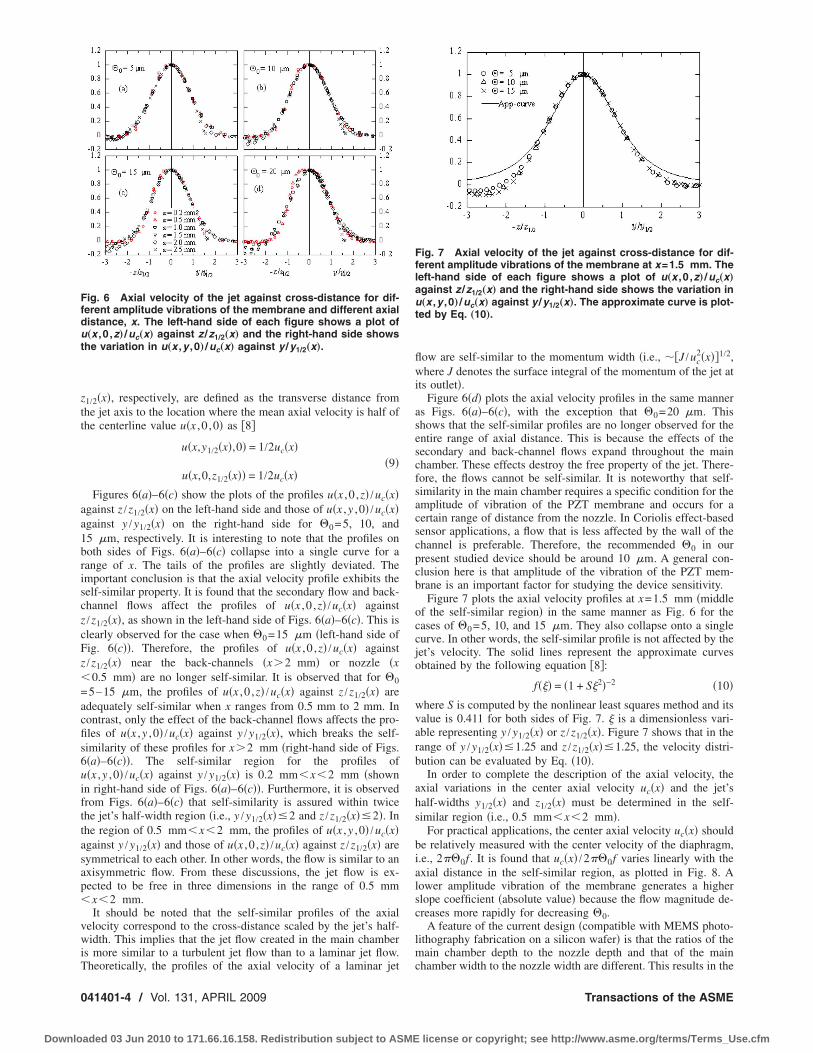
z1/2�x�, respectively, are defined as the transverse distance fromthe jet axis to the location where the mean axial velocity is half ofthe centerline value u�x ,0 ,0� as �8�

u�x,y1/2�x�,0� = 1/2uc�x��9�

u�x,0,z1/2�x�� = 1/2uc�x�

Figures 6�a�–6�c� show the plots of the profiles u�x ,0 ,z� /uc�x�against z /z1/2�x� on the left-hand side and those of u�x ,y ,0� /uc�x�against y /y1/2�x� on the right-hand side for �0=5, 10, and15 �m, respectively. It is interesting to note that the profiles onboth sides of Figs. 6�a�–6�c� collapse into a single curve for arange of x. The tails of the profiles are slightly deviated. Theimportant conclusion is that the axial velocity profile exhibits theself-similar property. It is found that the secondary flow and back-channel flows affect the profiles of u�x ,0 ,z� /uc�x� againstz /z1/2�x�, as shown in the left-hand side of Figs. 6�a�–6�c�. This isclearly observed for the case when �0=15 �m �left-hand side ofFig. 6�c��. Therefore, the profiles of u�x ,0 ,z� /uc�x� againstz /z1/2�x� near the back-channels �x2 mm� or nozzle �x�0.5 mm� are no longer self-similar. It is observed that for �0=5–15 �m, the profiles of u�x ,0 ,z� /uc�x� against z /z1/2�x� areadequately self-similar when x ranges from 0.5 mm to 2 mm. Incontrast, only the effect of the back-channel flows affects the pro-files of u�x ,y ,0� /uc�x� against y /y1/2�x�, which breaks the self-similarity of these profiles for x2 mm �right-hand side of Figs.6�a�–6�c��. The self-similar region for the profiles ofu�x ,y ,0� /uc�x� against y /y1/2�x� is 0.2 mm�x�2 mm �shownin right-hand side of Figs. 6�a�–6�c��. Furthermore, it is observedfrom Figs. 6�a�–6�c� that self-similarity is assured within twicethe jet’s half-width region �i.e., y /y1/2�x�2 and z /z1/2�x�2�. Inthe region of 0.5 mm�x�2 mm, the profiles of u�x ,y ,0� /uc�x�against y /y1/2�x� and those of u�x ,0 ,z� /uc�x� against z /z1/2�x� aresymmetrical to each other. In other words, the flow is similar to anaxisymmetric flow. From these discussions, the jet flow is ex-pected to be free in three dimensions in the range of 0.5 mm�x�2 mm.

It should be noted that the self-similar profiles of the axialvelocity correspond to the cross-distance scaled by the jet’s half-width. This implies that the jet flow created in the main chamberis more similar to a turbulent jet flow than to a laminar jet flow.Theoretically, the profiles of the axial velocity of a laminar jet

flow are self-similar to the momentum width �i.e., ��J /uc2�x��1/2,

where J denotes the surface integral of the momentum of the jet atits outlet�.

Figure 6�d� plots the axial velocity profiles in the same manneras Figs. 6�a�–6�c�, with the exception that �0=20 �m. Thisshows that the self-similar profiles are no longer observed for theentire range of axial distance. This is because the effects of thesecondary and back-channel flows expand throughout the mainchamber. These effects destroy the free property of the jet. There-fore, the flows cannot be self-similar. It is noteworthy that self-similarity in the main chamber requires a specific condition for theamplitude of vibration of the PZT membrane and occurs for acertain range of distance from the nozzle. In Coriolis effect-basedsensor applications, a flow that is less affected by the wall of thechannel is preferable. Therefore, the recommended �0 in ourpresent studied device should be around 10 �m. A general con-clusion here is that amplitude of the vibration of the PZT mem-brane is an important factor for studying the device sensitivity.

Figure 7 plots the axial velocity profiles at x=1.5 mm �middleof the self-similar region� in the same manner as Fig. 6 for thecases of �0=5, 10, and 15 �m. They also collapse onto a singlecurve. In other words, the self-similar profile is not affected by thejet’s velocity. The solid lines represent the approximate curvesobtained by the following equation �8�:

f�� = �1 + S�2�−2 �10�

where S is computed by the nonlinear least squares method and itsvalue is 0.411 for both sides of Fig. 7. � is a dimensionless vari-able representing y /y1/2�x� or z /z1/2�x�. Figure 7 shows that in therange of y /y1/2�x�1.25 and z /z1/2�x�1.25, the velocity distri-bution can be evaluated by Eq. �10�.

In order to complete the description of the axial velocity, theaxial variations in the center axial velocity uc�x� and the jet’shalf-widths y1/2�x� and z1/2�x� must be determined in the self-similar region �i.e., 0.5 mm�x�2 mm�.

For practical applications, the center axial velocity uc�x� shouldbe relatively measured with the center velocity of the diaphragm,i.e., 2��0f . It is found that uc�x� /2��0f varies linearly with theaxial distance in the self-similar region, as plotted in Fig. 8. Alower amplitude vibration of the membrane generates a higherslope coefficient �absolute value� because the flow magnitude de-creases more rapidly for decreasing �0.

A feature of the current design �compatible with MEMS photo-lithography fabrication on a silicon wafer� is that the ratios of themain chamber depth to the nozzle depth and that of the mainchamber width to the nozzle width are different. This results in the

Fig. 6 Axial velocity of the jet against cross-distance for dif-ferent amplitude vibrations of the membrane and different axialdistance, x. The left-hand side of each figure shows a plot ofu„x ,0 ,z… /uc„x… against z /z1/2„x… and the right-hand side showsthe variation in u„x ,y ,0… /uc„x… against y /y1/2„x….

Fig. 7 Axial velocity of the jet against cross-distance for dif-ferent amplitude vibrations of the membrane at x=1.5 mm. Theleft-hand side of each figure shows a plot of u„x ,0 ,z… /uc„x…against z /z1/2„x… and the right-hand side shows the variation inu„x ,y ,0… /uc„x… against y /y1/2„x…. The approximate curve is plot-ted by Eq. „10….



difference between y1/2�x� and z1/2�x�, as shown in Fig. 9. Thehalf-widths of the flow in the depth, z1/2�x�, appear to remainunchanged with axial distance, x, and their values are approxi-mately 0.2. Figure 9 also shows that the jet spreads along they-direction. The spread is approximately linear with a rate,dy1/2 /dx, of around 0.45–0.5.

The other flow components, v�x ,y ,z� and w�x ,y ,z�, along they- and z-directions, respectively, are also examined in the self-similar region �i.e., 0.5 mm�x�2 mm�. Similar to the exami-nation of the axial flow, v�x ,y ,z� /uc�x� and w�x ,y ,z� /uc�x� areplotted as functions of y /y1/2�x� and z /z1/2�x�, respectively, asshown in Fig. 10. The self-similar properties are not observed inthese cross section velocity components. The cross profiles,v�x ,y ,z� /uc�x� against z /z1/2�x� and w�x ,y ,z� /uc�x� againsty /y1/2�x�, approach zero. Physically, a circulatory flow is createdin the bracelet shape in the main chamber encompassing the jetflow, as shown in Fig. 11, which plots the mean velocity vector onthe horizontal and vertical planes. This also explains why the tailsof the axial velocity profiles against y /y1/2�x� or z /z1/2�x� are notself-similar. It is observed in Fig. 10 that v�x ,y ,z� and w�x ,y ,z�are of the same order of magnitude and are very small—less thanuc�x� by a factor of 25—as shown in Fig. 10. This implies that apassive scalar �e.g., temperature� is mainly transported by axialflow.

5 ConclusionsA simple device that is compatible with planar layer-by-layer

geometries and can create several jet flows within is proposed andnumerically studied by computational fluid dynamics. In thisstudy, four jet flows are independently formed. The principle ofthe device is presented.

The axial velocity component is self-similar with a cross-streamnondimensionlized by the half-widths of the jet flow if the ampli-tude of vibration of the PZT membrane lies in a suitable range.This implies that the spread of the jet flow along two perpendicu-lar directions is similar to a turbulent free jet flow. The self-similarregion covers almost the entire main chamber, except in areasvery close to the nozzle or the back-channels.

In the self-similar region, the jet flow is expected to vibratefreely in three dimensions.

Fig. 8 Variation in the center velocity against axial distance inthe self-similar region

Fig. 9 Variation of half-widths against axial distance in theself-similar region. Black symbols z1/2„x…, white symbolsy1/2„x…, circle �0=5 �m, upward-facing triangle �0=10 �m,and downward-facing triangle �0=15 �m.

Fig. 10 Variation of cross-stream velocity components withradial distance in the self-similar region. The left-hand side ofeach figure shows plots of v or w„x ,0 ,z… /uc„x… against z /z1/2„x…and the right-hand side shows the variation of v orw„x ,y ,0… /uc„x… against y /y1/2„x….

Fig. 11 Time averaged velocity fields on two perpendicularplanes containing the axis of the jet flow in the main chamber



The two remaining components of the flow are small as com-pared to the axial component.

Furthermore, the characteristics of the centerline axial velocity,as well as the half-widths of the jet, should be addressed in ageneral way. The device has been investigated only for one spe-cific dimension. Since the geometry, throat, and nozzle may con-tribute significantly in optimizing the operation of the device,these factors should be carefully considered in the future.

References�1� Woolley, A. T., Hadley, D., Landre, P., deMello, A. J., Mathies, R. A., and

Northrup, M. A., 1996, “Functional Integration of PCR Amplification andCapillary Electrophoresis in a Microfabricated DNA Analysis Device,” Anal.Chem., 68, pp. 4081–4087.

�2� Taylor, M. T., Nguyen, P., Ching, J., and Petersen, K. E., 2003, “Simulation of

Microfluidic Pumping in a Genomic DNA Blood-Processing Cassette,” J. Mi-cromech. Microeng., 13, pp. 201–208.

�3� Zhang, L., Koo, J. M., Jiang, L., Asheghi, M., Goodson, K. E., Santiago, J. G.,and Kenny, T. W., 2002, “Measurements and Modeling of Two-Phase Flow inMicrochannels With Nearly Constant Heat Flux Boundary Conditions,” J. Mi-croelectromech. Syst., 11, pp. 12–19.

�4� Dau, V. T., Dao, V. D., Shiozawa, T., Kumagai, H., and Sugiyama, S., 2005,“A Dual Axis Gas Gyroscope Utilizing Low Doped Silicon Thermistor,” 18thIEEE MEMS, pp. 626–629.

�5� Zhou, J., Yan, G., Zhu, Y., Xiao, Z., and Fan, J., 2005, “Design and Fabricationof a Microfluidic Angular Rate Sensor,” 18th IEEE International Conferenceon Micro Electro Mechanical Systems �MEMS�, pp. 363–366.

�6� Saito, K., Komatsu, G., and Kato, K., 2001, “An Analysis of Fluid Behavior onGas Angular Rate Sensor,” JSME Int. J., Ser. C, 67, pp. 135–140.

�7� Bassi, A., Gennar, F., and Symonds, P. S., 2003, “Anomalous Elastic-PlasticRespond to Short Pulse Loading of Circular Plates,” Int. J. Impact Eng., 28,pp. 65–91.

�8� Pope, S. B., 2000, Turbulent Flows, Cambridge University, Cambridge.



Pressurized Flow in a MesostructuredSilica Modified by Silane Groups

Venkata K. Punyamurtula

Aijie Han

Yu Qiao1


Department of Structural Engineering,University of California, San Diego,La Jolla, CA 92093-0085

By applying a quasihydrostatic pressure, water or electrolyte so-lution can be compressed into a surface treated MSU-H mesopo-rous silica. Based on the pressure-volume curves, thermodynamicand kinetic characteristics of the pressurized flow are analyzed.For pure water based system, continuum theory explains the test-ing data quite well but fails to capture the rate effect. For elec-trolyte solution based system, the classic interface theory breaksdown, probably due to the unique ion behaviors in thenanoenvironment. �DOI: 10.1115/1.3089542�

1 IntroductionLiquid behavior in nanoenvironment has been an important re-

search topic for more than a decade �1,2�, which shed much lighton fundamental mechanisms governing solid-liquid interactions atsmall length and time scales. The studies in this area have beenimmensely useful to developing better techniques for drug deliv-ery, micro-/nanotransportation, micro-/nanofabrication, biosens-ing, etc.

Over the years, energy dissipation associated with nanofluidicbehaviors has drawn considerable attention �3,4�. The initial ideawas based on the assumption that, as a liquid flows in nanoporesand the internal friction takes place across the large pore surface,the energy dissipation capacity can be ultrahigh. Such a systemmay have great applicability in advanced dampers, bumpers, andarmors. For instance, in an experiment performed by Li �5�, bend-ing moments were applied on a hydrophilic nanoporous silicablock soaked by water. As water flowed from compressive parts totensile parts, there was a detectable damping effect. However, theenergy dissipation efficiency was lower than the expected level.

Recently, an improved concept has been investigated by a fewresearch teams �6–11�, including the authors of this paper, whoreplaced the hydrophilic nanoporous solids by hydrophobic ones.Due to the capillary effect, as a hydrophobic nanoporous materialis immersed in water, the nanopores remain empty. Once a highpressure is applied on the liquid phase, pressure induced infiltra-tion �PII� would occur, accompanied by conversion of a signifi-cant amount of external work to excess solid-liquid interfacialenergy. In a number of nanoporous systems, the excess solid-liquid interfacial energy cannot be converted back to the hydro-static pressure as the external loading is removed; that is, thesorption isotherm curves are hysteretic, which results in ultrahighenergy dissipation efficiency larger than a few J/g, much betterthan many conventional protective materials �12�. A similar de-sign concept can be extended to nonpolar liquids using lyophobic

nanoporous materials, which has led to an even higher energydensity �13,14�. In these investigations, it has been noticed thatincreasing degree of hydrophobicity, decreasing pore size, andadding electrolytes can be of beneficial effects to improving sys-tem performance.

2 Experimental ProcedureIn the current study, we investigated a MSU-H type nanoporous

silica that was commonly used as adsorbent and catalyst support.It was of a hexagonal framework, small pore size, and relativelarge specific pore volume, ideal for energy absorption applica-tions. The network material was obtained from Sigma-Aldrich �St.Louis, MO� �CAT No. 643637�. The as-received material was inpowder form. The particle size was 20–80 �m. According to agas absorption analysis using a Tristar-3000 analyzer, the averagepore size was 7.1 nm, the specific pore volume was 0.9 cm3 /g,and the specific pore surface area was 510 m2 /g. Figure 1 showsthe Barrett–Joyner–Halenda �BJH� analysis result of nanoporevolume distribution. Its pore surface was hydrophilic, and there-fore could not be directly used for PII testing. In order to modifythe pore surface structure, the silica particles were first dried at100°C in a vacuum oven for 24 h and then refluxed in a silaneagent solution in a hot mantle. The solution was prepared by in-jecting 1 part of chlorotrimethylsilane into 40 parts of dry toluene.Prior to the refluxing, the mixture had been gently stirred at roomtemperature for 10 min. The refluxing time ranged from 3 h to 24h. During this process, the chlorotrimethylsilane molecules dif-fused into the nanopores and formed hydrophobic O–Si�CH3�3groups at nanopore walls, changing the surface wettability �15�.The treated sample was vacuum filtered, washed with dry toluene,and dried at 100°C for 24 h in vacuum.

Figure 2 depicts the PII experimental setup, which consisted of0.2 g of surface treated silica particles immersed in 7 g of liquid,a steel cylinder, and a piston. A compressive load was applied onthe liquid phase through the piston by an Instron machine, forcingthe piston into the cylinder at a constant rate. The liquid phase waseither de-ionized water or saturated aqueous solution of sodiumchloride. The compression rate, V, was 1–20 mm/min. The quasi-hydrostatic pressure in the liquid, p, was calculated as P /A0, withP being the axial load and A0=286 mm2 being the cross-sectionalarea of the cylinder. The piston displacement, �p, was also mea-sured, based on which the liquid volume change was calculated as�V0=�p ·A0. As the pressure exceeded 30–40 MPa, the piston wasmoved out of the cylinder at the same rate. Figures 3 and 4 showthe typical sorption isotherm curves. The resolutions of load anddisplacement measurements were 250 N and 20 �m, respectively.

3 Results and DiscussionWithout the surface treatment, the silica is hydrophilic and thus

the nanoporous particles can be infiltrated by water. Under thiscondition, as shown by the dashed curve in Fig. 3, no infiltrationcan be observed in the PII experiment. With the surface treatment,as shown by the solid curves, infiltration plateaus are formed. Theinfiltration plateau is defined as the middle portion of the loadingpart of sorption isotherm where the slope is much smaller thanthat of the linear compression sections. The surface treated nano-porous silica particles are initially filled by entrapped air. As thepressure is sufficiently high �4.5 MPa and 8.1 MPa for silicassurface treated for 3 h and 24 h, respectively�, liquid starts to enterthe largest nanopores. As a result, the system volume decreasesrapidly. As the pressure rises, smaller nanopores are involved inthe PII process, during which the entrapped gas molecules aredissolved by the confined liquid. Note that the interactions amonggas and liquid molecules in a nanopore can be fundamentallydifferent from that in a bulk phase, as demonstrated by the mo-lecular dynamics simulation in Ref. �16�. As the nanopore wallconfines the molecular motion, there must be a sufficiently large“gap” between the gas molecule and the solid surface; otherwise,


JOURNAL OF FLUIDS ENGINEERING. Manuscript received February 23, 2007; final manu-script received March 11, 2008; published online March 6, 2009. Assoc. Editor: AliBeskok.



the liquid molecules would be blocked. When the pressure is low-ered, since gas phase nucleation may be energetically unfavorable,the confined liquid does not come out of the nanopores �17�; thatis, a decrease in solid-liquid interfacial energy associated with theexpansion of a nanobubble can be lower than the energy requiredfor “evaporating” molecules from liquid phase to vapor phase,which causes a significant hysteresis in sorption isotherm. Theenclosed area of the loading-unloading cycle indicates the dissi-pated energy �Table 1�.

According to Fig. 3, the infiltration volume of the silica surfacetreated for 3 h, which can be measured by the width of infiltration

plateau, is about 0.7 cm3 /g, smaller than the BJH measurementresult of nanopore volume of untreated silica. Note that the mo-lecular size of O–Cl�CH3�3 is around 0.26 nm. As the nanoporesurface is covered by a surface group layer, the effective pore sizeshould be reduced from 7.1 nm to 6.6 nm, and the effective porevolume would decrease by about 15%, from 0.9 cm3 /g to0.76 cm3 /g, quite close to the infiltration volume. The effectivesolid-liquid interfacial tension, according to the classic Young’sequation, can be calculated as ��= pin ·r /2=13 mJ /m2, with pinbeing taken as 7.9 MPa and r=3.3 nm.

As the surface treatment time, tr, is increased to 24 h, the infil-tration pressure largely rises to 12.4 MPa, while the infiltrationvolume decreases considerably from 0.7 cm3 /g to 0.4 cm3 /g,even though the nanoporous structure does not change. This phe-nomenon may be attributed to the formation of dense layers ofsilane groups at nanopore surfaces. When the surface coverage issaturated, in a prolonged surface treatment process, chlorotrimeth-ylsilane molecules would continue to diffuse into the nanopores.Consequently, the pore volume decreases. The reduction in acces-sible pore volume from 0.7 cm3 /g to 0.4 cm3 /g is equivalent toa change in effective nanopore radius from 3.3 nm to 2.5 nm. Withthe same solid-liquid interfacial tension of 13 mJ /m2, the infiltra-tion pressure would increase from 7.9 MPa to 10.5 MPa, which isquite close to the values shown in Fig. 3. That is, the large varia-tion in infiltration pressure and volume associated with the in-crease in treatment time are caused by the decrease in emptynanopore space.

If the liquid motion in nanopores could be described by a cir-cular Poiseuille flow, as the infiltrating liquid molecules movealong the pore wall, an additional pressure must be applied toovercome the viscosity effect. For a zero-order approximation, thepressure increase can be assessed as dp=32� ·v ·dz /D2 �18�,where �=10−3 Pa s is the liquid viscosity, v is the inflow rate, dzis the pore depth, and D=6.6 nm is the effective pore diameterfor the silica sample that is treated for 3 h. In the current study, thecross-sectional area of the testing cylinder, A0, is 286 mm2, andtherefore it takes about 30 s to fill the nanopores. The averagesilica particle size is about 50 �m. Thus, the inflow rate, v, is

Fig. 1 The BJH analysis result of the nanopore volumedistribution

Fig. 2 A schematic of the testing system

Fig. 3 Typical sorption isotherm curves of pure water basedsystem. The specific system volume change is defined as thesystem volume change normalized by the mass of the nano-porous silica.

Specific System Volume Change (cm3/g)

Pressure(MPa)

Sodium ChlorideSolution Based System

Pure WaterBased System

Fig. 4 The effect of addition of sodium chloride. The silica issurface treated for 3 h.

Table 1 Energy absorption capacity of surface treated MSU-Hsilica „J/g…

Experimental condition

Surface treatment time �h�

3 12 24

v=1 mm /minIn pure water 5.1 5.6 3.1In saturated NaCl solution 6.8 7.0 3.6

v=20 mm /min �in pure water� 5.2 5.6 3.2



around 1 �m /s, and the characteristic value of dz is about10 �m. Consequently, when the piston speed changes from 1mm/min to 20 mm/min, the sorption isotherm curve should shiftalong the pressure axis by a few MPa, which was not observed inthe PII experiment. When the loading rate varied in this range, theinfiltration plateaus were nearly identical. Clearly, in the confiningnanoenvironment, the no-slip boundary condition is no longervalid, and the definition of liquid viscosity breaks down, whichexplains why the internal-friction-based energy dissipationmechanism did not have the expected energy density �5�.

As sodium chloride is added in the liquid phase, as shown inFig. 4, while the infiltration volume does not vary, the infiltrationpressure becomes much higher. The pin increase is about 2.2 MPa,which corresponds to a large variation in effective solid-liquidinterfacial tension of about 8.6 mJ /m2, 66% of that of pure water.Note that the surface tension of saturated sodium chloride solutionis larger than that of pure water by less than 10% �19�. The largeincrease in the effective interface tension should be related to theconfinement effect of pore walls on ion distribution. In a nano-pore, normal to the pore surface, there is no enough space for theformation of a double layer. The bulk phase may not exist. There-fore, the effective ion concentration is higher than that at a largesolid surface; that is, the ion structure is affected by the oppositenanopore surface, causing a “squeezing” effect, which can lead toa higher liquid composition sensitivity. The details of the funda-mental mechanisms are still under investigation.

4 ConclusionTo summarize, through a pressure induced infiltration experi-

ment on a surface treated MSU-H nanoporous silica, the liquidmotion in nanopores are examined. For the system under investi-gation, the classic capillary theory can be employed to relate theinfiltration pressure to the nanopore size. However, the continuumtheory does not explain the low sensitivity of sorption isotherm toloading rate. It also fails to capture the large variation in infiltra-tion pressure caused by addition of sodium chloride.

AcknowledgmentThis work was supported by the Army Research Office under

Grant No. W911NF-05-1-0288, for which the authors are gratefulto Dr. D.M. Stepp.

References�1� Sansom, M. S. P., and Biggin, P. C., 2001, “Biophysics: Water at the Nano-

scale,” Nature �London�, 414, pp. 156–158.�2� Majumder, M., Chopra, N., Andrews, R., and Hinds, B. J., 2005, “Experimen-

tal Observation of Enhanced Liquid Flow Through Aligned Carbon NanotubeMembranes,” Nature �London�, 438, pp. 44–46.

�3� Borman, V. D., Grekhov, A. M., and Troyan, V. I., 2000, “Investigation of thePercolation Transition in a Nonwetting Liquid-Nanoporous Medium System,”J. Exp. Theor. Phys., 91, pp. 170–181.

�4� Fadeev, A. Y., and Eroshenko, V. A., 1997, “Study of Penetration of Water IntoHydrophobized Porous Silicas,” J. Colloid Interface Sci., 187, pp. 275–282.

�5� Li, J. C. M., 2000, “Damping of Water Infiltrated Nanoporous Glass,” J. AlloysCompd., 310, pp. 24–29.

�6� Martin, T., Lefevre, B., Brunel, D., Galarneau, A., Di Renzo, F., Fajula, F.,Gobin, P. F., Quinson, J. F., and Vigier, G., 2002, “Dissipative Water Intrusionin Hydrophobic MCM-41 Type Materials,” Chem. Commun. �Cambridge�,2002, pp. 24–25.

�7� Borman, V. D., Belogorlov, A. A., Grekhov, A. M., Lisichkin, G. V., Tronin, V.N., and Troyan, V. I., 2005, “The Percolation Transition in Filling a Nano-porous Body by a Nonwetting Liquid,” J. Exp. Theor. Phys., 100, pp. 385–397.

�8� Surani, F. B., Kong, X., and Qiao, Y., 2005, “Two-Staged Sorption Isotherm ofa Nanoporous Energy Absorption System,” Appl. Phys. Lett., 87, p. 251906.

�9� Surani, F. B., Kong, X., Panchal, D. B., and Qiao, Y., 2005, “Energy Absorp-tion of a Nanoporous System Subjected to Dynamic Loadings,” Appl. Phys.Lett., 87, p. 163111.

�10� Kong, X., and Qiao, Y., 2005, “Improvement of Recoverability of a Nano-porous Energy Absorption System by Using Chemical Admixture,” Appl.Phys. Lett., 86, p. 151919.

�11� Kong, X., Surani, F. B., and Qiao, Y., 2005, “Effects of Addition of Ethanol onthe Infiltration Pressure of a Mesoporous Silica,” J. Mater. Res., 20, pp. 1042–1045.

�12� Lu, G., and Yu, T., 2003, Energy Absorption of Structures and Materials, CRC,Boca Raton, FL.

�13� Punyamurtula, V. K., and Qiao, Y., 2007, “Hysteresis of Sorption Isotherm ofa Multiwall Carbon Nanotube in Paraxylene,” Mater. Res. Innovations, 11, pp.37–39.

�14� Punyamurtula, V. K., Han, A., and Qiao, Y., 2007, Damping Properties ofNanoporous Carbon-Cyclohexane Mixtures,” Adv. Eng. Mater., 9, pp. 209–211.

�15� Lim, M. H., and Stein, A., 1999, “Comparative Studies of Grafting and DirectSyntheses of Inorganic-Organic Hybrid Mesoporous Materials,” Chem. Mater.,11, pp. 3285–3295.

�16� Qiao, Y., Cao, G., and Chen, X., 2007, “Effects of Gas Molecules on Nano-fluidic Behaviors,” J. Am. Chem. Soc., 129, pp. 2355–2359.

�17� Han, A., Kong, X., and Qiao, Y., 2006, “Pressure Induced Infiltration in Nano-pores,” J. Appl. Phys., 100, p. 014308.

�18� Fay, J. A., 1994, Introduction to Fluid Mechanics, MIT, Cambridge, MA.�19� Hartland, S., 2004, Surface and Interface Tension, CRC, Boca Raton, FL.



j.fluids.engineering.2009.vol.131.n4

Documents

new address

new york

address changes

changes of address

numerical simulation

copyright act

brian thomas

maul041102 dynamic model