1

AME 30315; Spring 2015; Midterm 2 Review (not graded)

Problems:

• 9.3

• 9.8

• 9.9

• 9.12 except parts 5 and 6.

• 9.13 except parts 4 and 5

• 9.28

• 9.34

• You are given the transfer function:

G(s) =−100

(s+ 10) (s+ 100)e−0.5s.

1) Plot the bode plot for G(s)

2) Find the analytic solution to |G(iω)| and ∠ (G(iω)).

• Plot the bode plot for the transfer function:

G(s) =s− 100

(s+ 10) (s+ 100).

• (A)

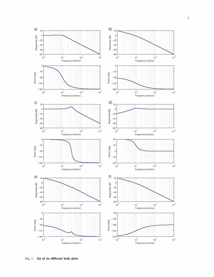
1) Below are pole and zero locations for five different transfer functions G(s). Match the

pole and zero locations to the corresponding bode plots in Fig. 1. You do not need

to perform any calculations to receive full credit; however, you do need to provide a

complete justification.

Notes: (i)

2

a) There are more bode plots than pole/zero sets, so one bode plot will not have a

match;

b) (s+ 5− 8.66i) (s+ 5 + 8.66i) = s2 + 10s+ 100;

c) (s+ 5− 29.58i) (s+ 5 + 29.58i) = s2 + 10s+ 900;

d) (s+ 5− 31.23i) (s+ 5 + 31.23i) = s2 + 10s+ 1000.

1) z = [−5± 29.58i], p = [0,−10,−5± 31.23i]: match = ; Justification:

2) z = none; p = [−5± 8.66i]: match = ; Justification:

3) z = none; p = [0,−10]: match = ; Justification:

4) z = none; p = [0, 10]: match = ; Justification:

5) z = none; p = [−5± 29.58i]: match = ; Justification:

3

100

101

102

103

−80

−60

−40

−20

0

20

Frequency [rad/sec]

Mag

nitu

de [d

B]

100

101

102

103

−180

−135

−90

−45

0

Frequency [rad/sec]

Phas

e [d

eg]

100

101

102

103

−80

−60

−40

−20

0

20

Frequency [rad/sec]

Mag

nitu

de [d

B]

100

101

102

103

−180

−135

−90

−45

0

Frequency [rad/sec]

Phas

e [d

eg]

100

101

102

103

−80

−60

−40

−20

0

20

Frequency [rad/sec]

Mag

nitu

de [d

B]

100

101

102

103

−180

−135

−90

−45

0

Frequency [rad/sec]

Phas

e [d

eg]

100

101

102

103

−80

−60

−40

−20

0

20

Frequency [rad/sec]

Mag

nitu

de [d

B]

100

101

102

103

−90

−45

0

45

90

Frequency [rad/sec]

Phas

e [d

eg]

100

101

102

103

−80

−60

−40

−20

0

20

Frequency [rad/sec]

Mag

nitu

de [d

B]

100

101

102

103

−180

−135

−90

−45

0

Frequency [rad/sec]

Phas

e [d

eg]

100

101

102

103

−80

−60

−40

−20

0

20

Frequency [rad/sec]

Mag

nitu

de [d

B]

100

101

102

103

−270

−225

−180

−135

−90

Frequency [rad/sec]

Phas

e [d

eg]

a)

d)

f )e)

c)

b)

Fig. 1. Set of six different bode plots.

4

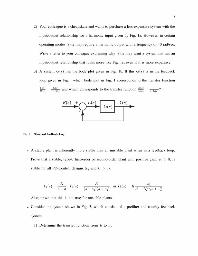
2) Your colleague is a cheapskate and wants to purchase a less-expensive system with the

input/output relationship for a harmonic input given by Fig. 1a. However, in certain

operating modes (s)he may require a harmonic output with a frequency of 40 rad/sec.

Write a letter to your colleague explaining why (s)he may want a system that has an

input/output relationship that looks more like Fig. 1c, even if it is more expensive.

3) A system G(s) has the bode plot given in Fig. 1b. If this G(s) is in the feedback

loop given in Fig. , which bode plot in Fig. 1 corresponds to the transfer function

Y (s)R(s)

= G(s)1+G(s)

and which corresponds to the transfer function E(s)R(s)

= 11+G(s)

?

R(s)G(s)

+

-E(s) Y(s)

Fig. 2. Standard feedback loop.

• A stable plant is inherently more stable than an unstable plant when in a feedback loop.

Prove that a stable, type-0 first-order or second-order plant with positive gain, K > 0, is

stable for all PD-Control designs (kp and kd > 0):

P1(s) =K

s+ a; P2(s) =

K

(s+ a1)(s+ a2); or P3(s) = K

ω2n

s2 + 2ζωns+ ω2n

Also, prove that this is not true for unstable plants.

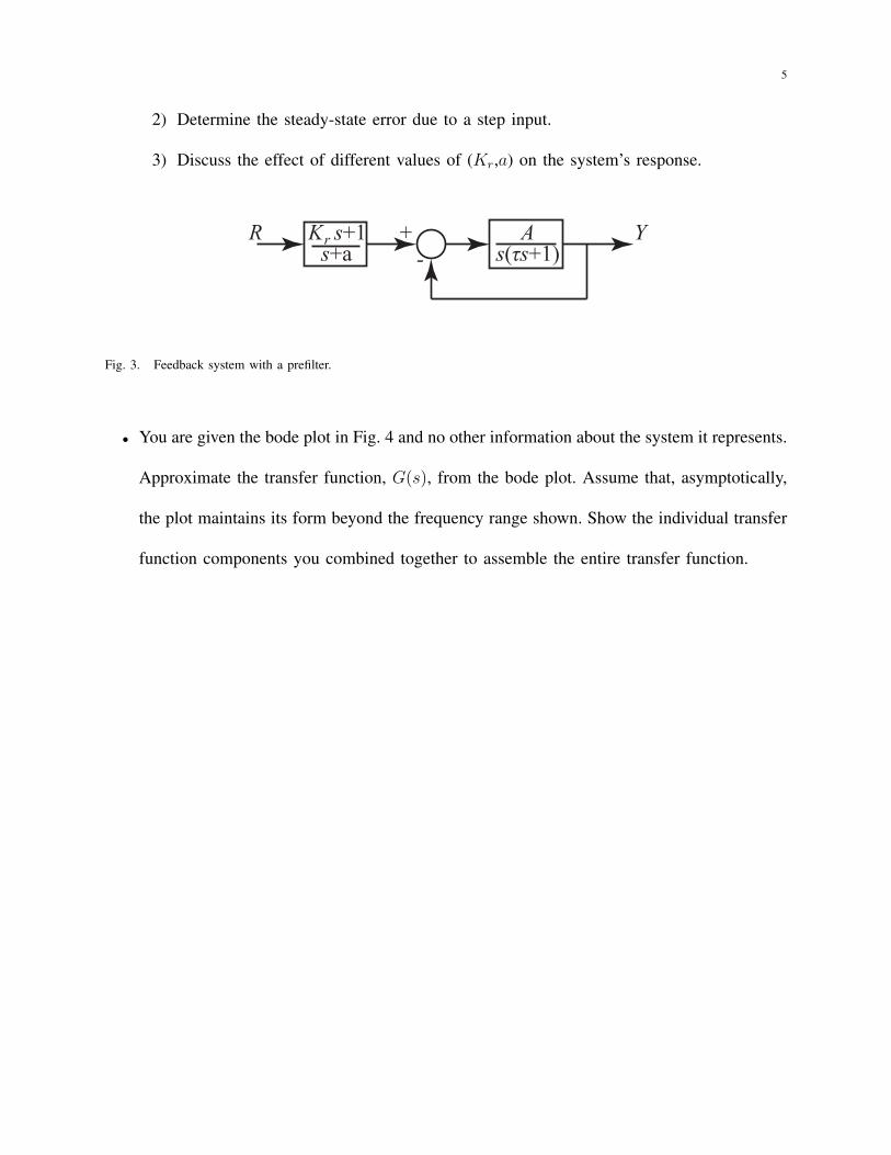
• Consider the system shown in Fig. 3, which consists of a prefilter and a unity feedback

system.

1) Determine the transfer function from R to Y .

5

2) Determine the steady-state error due to a step input.

3) Discuss the effect of different values of (Kr,a) on the system’s response.

K s+1rs+a

As(τs+1)

R Y+-

Fig. 3. Feedback system with a prefilter.

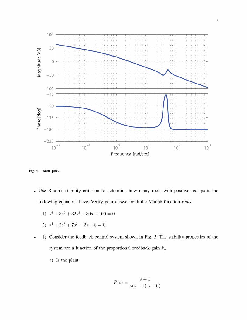
• You are given the bode plot in Fig. 4 and no other information about the system it represents.

Approximate the transfer function, G(s), from the bode plot. Assume that, asymptotically,

the plot maintains its form beyond the frequency range shown. Show the individual transfer

function components you combined together to assemble the entire transfer function.

6

−100

−50

0

50

100M

agni

tude

[dB]

10−2

10−1

100

101

102

103

−225

−180

−135

−90

−45

Phas

e [d

eg]

Frequency [rad/sec]

Fig. 4. Bode plot.

• Use Routh’s stability criterion to determine how many roots with positive real parts the

following equations have. Verify your answer with the Matlab function roots.

1) s4 + 8s3 + 32s2 + 80s+ 100 = 0

2) s4 + 2s3 + 7s2 − 2s+ 8 = 0

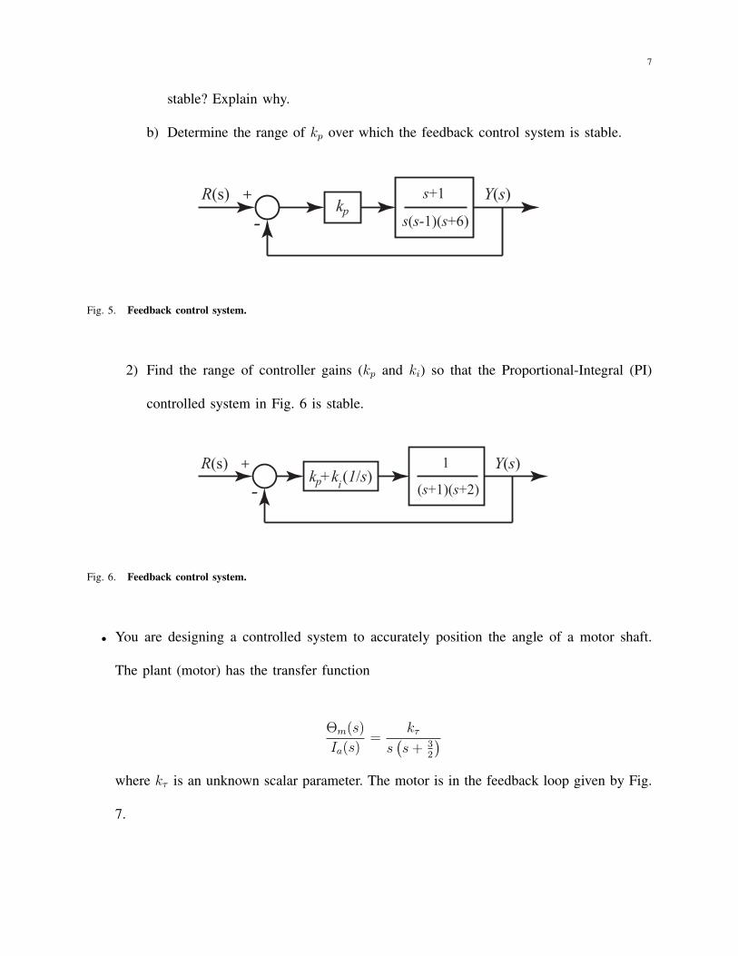
• 1) Consider the feedback control system shown in Fig. 5. The stability properties of the

system are a function of the proportional feedback gain kp.

a) Is the plant:

P (s) =s+ 1

s(s− 1)(s+ 6)

7

stable? Explain why.

b) Determine the range of kp over which the feedback control system is stable.

R(s) Y(s)+

-s+1

s(s-1)(s+6)k p

Fig. 5. Feedback control system.

2) Find the range of controller gains (kp and ki) so that the Proportional-Integral (PI)

controlled system in Fig. 6 is stable.

R(s) Y(s)k +k (1/s)

+

-1

(s+1)(s+2)p i

Fig. 6. Feedback control system.

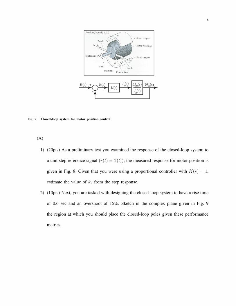
• You are designing a controlled system to accurately position the angle of a motor shaft.

The plant (motor) has the transfer function

Θm(s)

Ia(s)=

kτ

s(s+ 3

2

)where kτ is an unknown scalar parameter. The motor is in the feedback loop given by Fig.

7.

8

R(s) Θ (s)mI (s)

K(s)Θ (s)m

a

+

-E(s) I (s)a

(Franklin, Powell, 2002)

Fig. 7. Closed-loop system for motor position control.

(A)

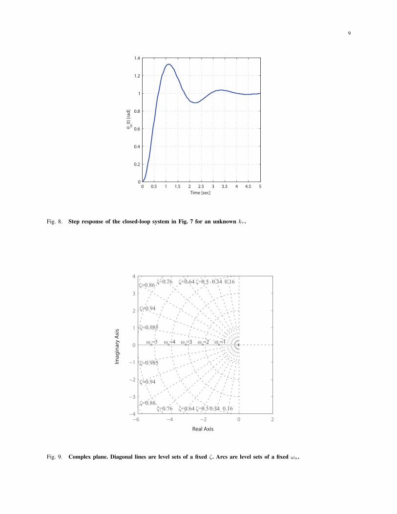
1) (20pts) As a preliminary test you examined the response of the closed-loop system to

a unit step reference signal (r(t) = 1(t)); the measured response for motor position is

given in Fig. 8. Given that you were using a proportional controller with K(s) = 1,

estimate the value of kτ from the step response.

2) (10pts) Next, you are tasked with designing the closed-loop system to have a rise time

of 0.6 sec and an overshoot of 15%. Sketch in the complex plane given in Fig. 9

the region at which you should place the closed-loop poles given these performance

metrics.

9

0 0.5 1 1.5 2 2.5 3 3.5 4 4.5 50

0.2

0.4

0.6

0.8

1

1.2

1.4

Time [sec]

θ (t

) [ra

d] m

Fig. 8. Step response of the closed-loop system in Fig. 7 for an unknown kτ .

−6 −4 −2 0 2−4

−3

−2

−1

0

1

2

3

40.160.34ζ=0.5ζ=0.64ζ=0.76ζ=0.86

ζ=0.94

ζ=0.985

0.160.34ζ=0.5ζ=0.64ζ=0.76ζ=0.86

ζ=0.94

ζ=0.985

ω =1ω =2ω =3ω =4ω =5

Real Axis

Imag

inar

y A

xis

n n n n n

Fig. 9. Complex plane. Diagonal lines are level sets of a fixed ζ. Arcs are level sets of a fixed ωn.

10

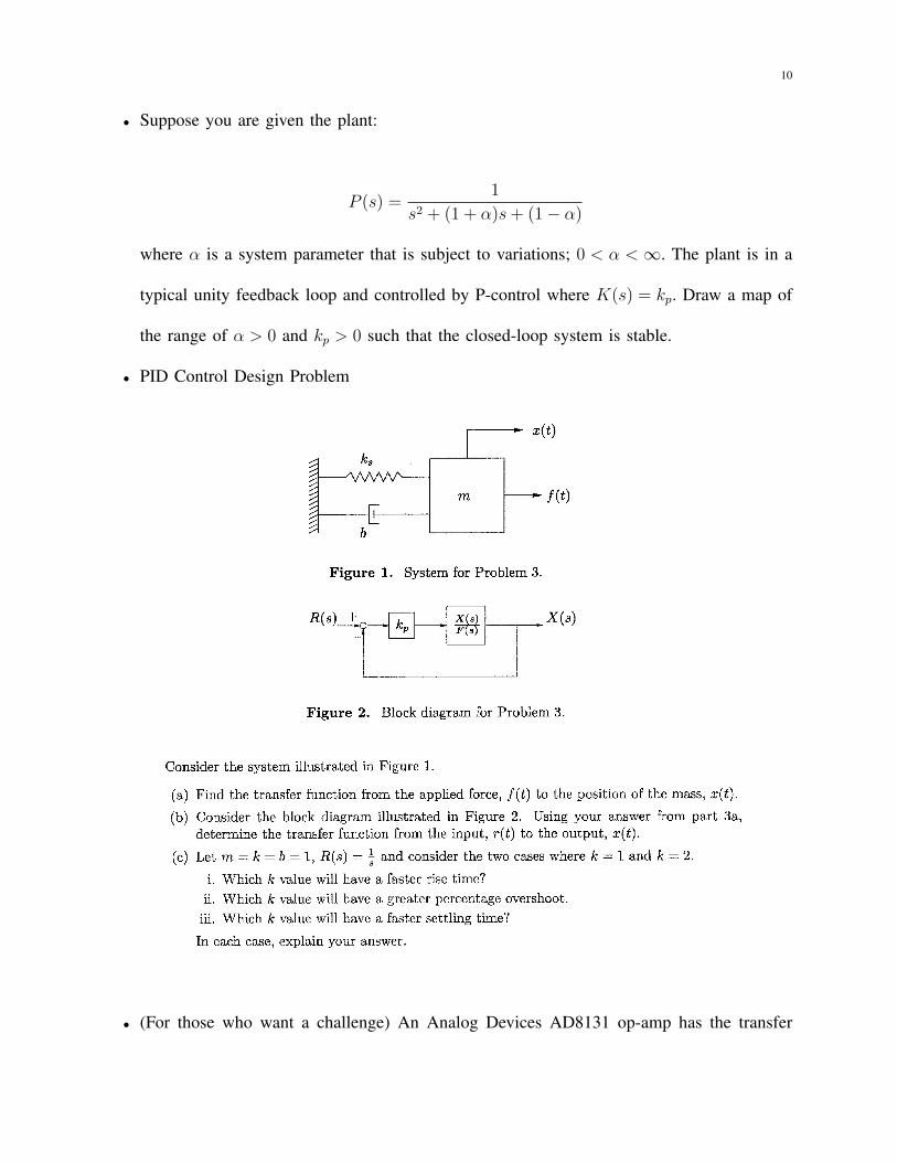
• Suppose you are given the plant:

P (s) =1

s2 + (1 + α)s+ (1− α)

where α is a system parameter that is subject to variations; 0 < α <∞. The plant is in a

typical unity feedback loop and controlled by P-control where K(s) = kp. Draw a map of

the range of α > 0 and kp > 0 such that the closed-loop system is stable.

• PID Control Design Problem

• (For those who want a challenge) An Analog Devices AD8131 op-amp has the transfer

11

function:

G(s) =−2(

s2π475×106 + 1

)2 .1) Find the analytic solution for |G(iω)| and ∠(G(iω)).

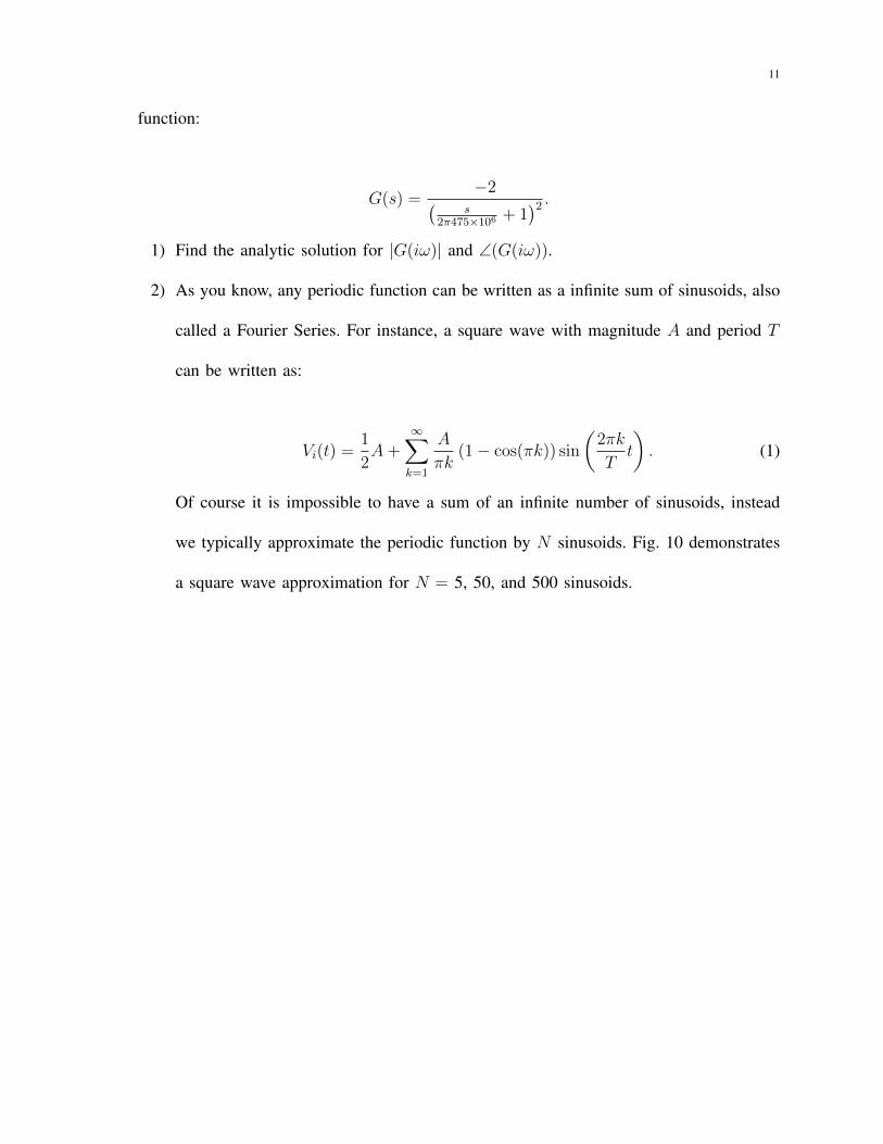
2) As you know, any periodic function can be written as a infinite sum of sinusoids, also

called a Fourier Series. For instance, a square wave with magnitude A and period T

can be written as:

Vi(t) =1

2A+

∞∑k=1

A

πk(1− cos(πk)) sin

(2πk

Tt

). (1)

Of course it is impossible to have a sum of an infinite number of sinusoids, instead

we typically approximate the periodic function by N sinusoids. Fig. 10 demonstrates

a square wave approximation for N = 5, 50, and 500 sinusoids.

12

0 T 2T

0

A

Time [msec]

Vi(t

) [V]

N = 5N = 50N = 500

Fig. 10. Approximation of a square wave with N sinusoids.

Given your analytic solution from Part 1, write the analytic solution for the output,

Vo(t), given that the input is the infinite sum in Equation (1).

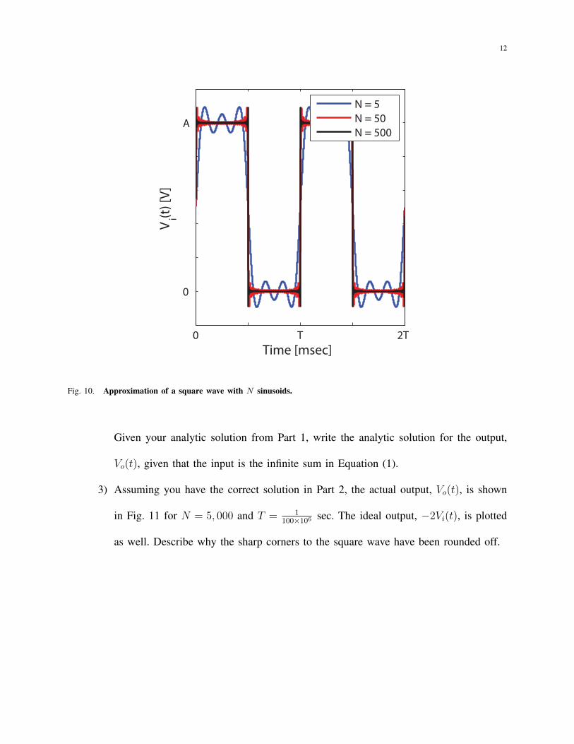
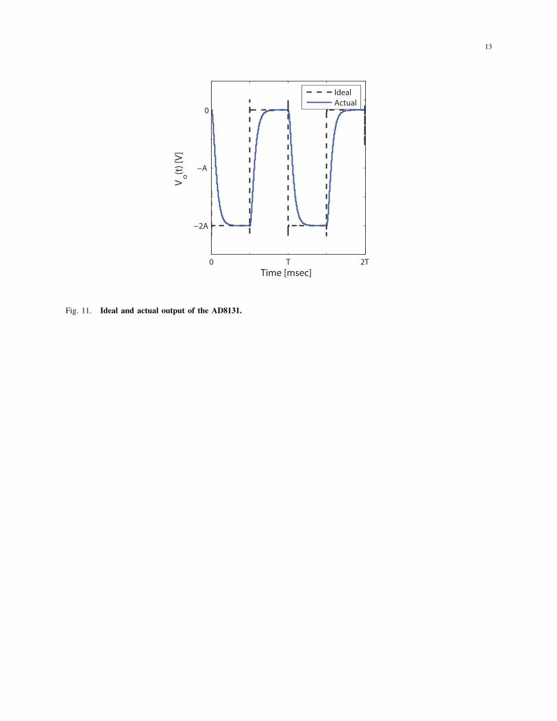
3) Assuming you have the correct solution in Part 2, the actual output, Vo(t), is shown

in Fig. 11 for N = 5, 000 and T = 1100×106 sec. The ideal output, −2Vi(t), is plotted

as well. Describe why the sharp corners to the square wave have been rounded off.

13

0 T 2T

−2A

−A

0

Time [msec]

Vo(t

) [V]

IdealActual

Fig. 11. Ideal and actual output of the AD8131.