jjee pages 253-269 jordan journal of electrical

JJEE Volume 2, Number 3, 2016 Pages 253-269

Jordan Journal of Electrical Engineering ISSN (Print): 2409-9600, ISSN (Online): 2409-9619

Corresponding author's e-mail: [email protected]

Excitation Control of a Synchronous Generator Using Neural

Networks and Simulated Annealing Controllers

Ali S. Al-Dmour Department of Electrical Engineering, Mu'tah University, Al-Karak, Jordan

e-mail: [email protected]

Received: February 13, 2016 Accepted: March 9, 2016 Abstract— This paper considers the problem of oscillations in a synchronous generator connected to infinite bus through transmission lines. Two on-line control techniques, namely, artificial neural networks (ANN) and simulated annealing (SA) are utilized to cancel the oscillations in synchronous generators (SG). Simulation results of applying external disturbances to the synchronous generator controlled by the proposed simulated annealing controllers are compared to results obtained by using neural network controllers. These control schemes contribute to preventing system instability by suppressing the low-frequency oscillations arising from power grid fault disturbances. The proposed on-line SA and NN integrate a voltage regulator and a power system stabilizer to obtain near-optimal solutions of the problem through utilizing functions evaluation. They can be adopted to replace the conventional automatic voltage regulator (AVR) with power system stabilizer (PSS) of the generator. Simulation results show that algorithms can efficiently and effectively solve such optimization problems within short time. In addition, they are presented to demonstrate the effectiveness and advantage of the control system of synchronous generator (SG) in comparison with the conventional control scheme so as to allow the generator to operate closely to its steady state stability limits. Keywords— Excitation control, Neural networks, On-line control, Optimization, Simulated annealing, Synchronous generator.

I. INTRODUCTION

Successful operation of modern complex power system depends largely on the engineer’s ability to provide a reliable and uninterrupted service to the load, ideally with best quality. The load must be fed at a constant voltage; and frequency must be held within close tolerances so that the consumer's equipment may operate satisfactorily [1]. It is important to observe that change in the real output power of electric generators affect essentially, only the frequency; and change in the reactive power affect essentially, only the voltage in the system. These properties make it possible to divide the control of a power system into two separate control channels, the MEGAVAR voltage control channel and the MEGAWATT frequency control channel. According to this classification, a generator is equipped with two major controls. Automatic Voltage Regulator (AVR) maintains the generator voltage to a reference value; and a governor keeps the generator rotating speed or frequency constant. However, most electric power systems are equipped with (AVR) and (AGC) controls, but still they have spontaneous oscillations at very low frequencies in order of several cycles per minute. The low frequency oscillation is an unstable phenomenon. It belongs to the so-called small signal stability problem in power systems. Also, the system suffers from large oscillations due to transient changes, faults and other types of disturbances. A small signal (steady-state) stability problem arises when a generator or a group of generators in a power system is subjected to small and gradual changes in load. This leads to unbalance between the mechanical input and electrical output powers of the generator. Following a small disturbance, if system variables (frequency, power, and voltage) do not reach their steady-state values at specified levels and time, poorly damped or even unstable low frequency oscillations occur in these variables [2], [3].

254 © 2016 Jordan Journal of Electrical Engineering. All rights reserved - Volume 2, Number 3

The requirement of a reliable power system is to operate the SG in a large area interconnection network. Effective control makes dynamic operations stable when there is a small variation or small oscillation in the network or in the excitation and governor control systems, as well as when it is subjected to large and sudden disturbance [4]. This is called transient stability of synchronous machine. These disturbances, which include a fault, a heavily loaded line or a bruit of large load, may also cause instability. Permanent changes, such as load changes, usually alter the system at least temporarily so that the subsequent steady-state operation will be different from that prior to the disturbance [1], [5]. In this paper, neural networks with specialized learning and simulated annealing (SA) approaches for problem optimization control are presented. Artificial neural networks (ANNs) are adaptive non-linear maps that accept inputs from one finite dimensional space and produce outputs in another finite space. This inherent nonlinearity makes them very useful tools in complex, uncertain and dynamic environments [6], [7]. The power grid is highly complex, uncertain and dynamic in which ANNs have proved to be useful in providing effective control [8]. It has been reported that when using specialized learning, it is beneficial to implement off-line learning first. The first rough approximation of the desired control law is performed via direct learning [9]. In this paper, the neural controller would be capable for driving the system over the entire operating range without instability problems. After this has been done, it will be possible to implement the on-line specialized learning to improve the NN controller. ANNs have been used in a wide range of applications, such as modeling tools, for regression, classification, and system approximation [10], [11], [12]. They are also attractive nonlinear controllers due to their inherent nonlinearity, insensitivity to noise and robustness [13], [14]. Research on the use of ANNs for automatic voltage regulation has been explored using recurrent neural networks (RNN), which show a better performance than the conventional AVR with PSS [15], [16], [17]. Extensive work has also been done on the use of ANNs in adaptive critic design (ACD) used for synchronous generator voltage regulation. In our work, the NN controller is investigated using the specialized learning. In addition, the results of the implementation of NN controller and the on-line simulated annealing are presented and compared. Simulated Annealing (SA) is a well-known probabilistic meta-heuristic; and it can be used to solve discrete and continuous optimization problems. The significant advantage of SA over other solution methods has made it a practical solution method for solving complex optimization problems. In this study, SA is used to minimize a prescribed objective function. It should be noted that on-line SA algorithm is run several times, before optimal control signals are obtained. In this paper, the on-line neuro-controller with specialized learning and SA are designed to replace the conventional AVR with PSS. Simulation results show that the performance of SA controllers based excitation system is superior to that of a conventional AVR and PSS excitation system.

II. SYNCHRONOUS GENERATOR MODELING

For any electric power system dynamic study, a proper mathematical model must be chosen. Yet, the selection of a power system model cannot be dissociated from the problem itself, or from the computational facilities and control techniques available. It is neither adequate nor practical to revise "universal models" for all power system dynamic problems [18]. When the power system stability problem was investigated using an ac calculating board years ago, the model of voltage behind reactance with a second-order torque equation was the best choice; the system was relatively small; and there were no other computational facilities

© 2016 Jordan Journal of Electrical Engineering. All rights reserved - Volume 2, Number 3 255

available. With modern digital computers, however, there is a tendency to over-represent an electric power system [1]. There are various kinds of power system dynamic problems: high-or low frequency oscillations, large or small (fast and slow varying) disturbances, and large or small electric power systems. However, there is only a limited number of system components that are essential to the dynamic study: the hydraulic and steam turbines, the synchronous generator, the governor, and the excitation system. For each of them, several basic models are recommended by the professional societies for the study of specific problems [19]. When studying the identification and control of synchronous machines, it is necessary to have a mathematical model for it. The model may be obtained in the form of a set of differential equations. The state space representation is the most suitable technique for digital computer applications in synchronous machine control. Such models can be obtained from the knowledge of the physical behavior of the system or from input-output data. A dynamic system consisting of a finite number of lumped elements may be described by ordinary differential equations in which time is the independent variable. By using vector matrix notation, nth order differential equation may be expressed as nth order vector-matrix of the first order differential equation. If n-element of the vector-matrix differential equation is a set of state variables, the vector-matrix differential equation will be called a state equation. [2]. It should be noted that the list of symbols of all parameters and variables of the adopted system is presented in Table A1. The nonlinear time-invariant system equations for the system are of form:

),( uxfx = (1)

FFdod

do

d

ddoF V

XX

XXXV

dtd ∆ψ∆

τδ∆δψ∆

Σ

Σ

Σ

+

′′

−

′

′−−= sin)(

(2)

ω∆ωωδ∆ =−= sdtd

(3)

mFdod

oo

dq

oqd

dod

Fooo

PXM

V

XXVXX

XV

Mdtd

+

′′

−

′−′

+′′

−=

ψ∆τδ

δ∆δ

τψδ

ω∆

Σ

ΣΣΣ

sin

2cos)(cos1 2

(4)

exs

ss

ss UGVV

dtd

ττ+−=

1

(5)

se

eF

eF

dod

qo

toe

e

od

dqoo

q

qdo

toe

oeF

VGVX

xVV

G

XxV

XxV

VVGV

dtd

∆τ

∆τ

ψ∆ττ

δ∆δδτ

∆Σ

−

−

′

−

′

′−

−=

∑

∑

1

sincos

(6)

Ft KKV ψ∆δ∆∆ 21 += (7)

′

′−= o

dto

odqoo

qto

oqdo

XVVXV

XVVXV

K δδ sincos1

(8)


′′

=ddoto

qo

XVXV

Kτ2

(9)

On this basis, (2), (3), (4) and (7) represent the four state equations of the synchronous machine; and flux linkage (ψ F ) is a state variable to obtain a simple formulation [2], [1]. Equations (5) and (6) represent the state equation of a second order exciter voltage regulator system. Therefore, the overall state-space equation will be:

+

∆∆∆∆∆∆

−

=

∆

∆

∆

∆

∆

∆

•

•

•

•

•

•

PU

VV

V

aaaaa

aaKaaa

aMD

a

Vs

V

V

m

ex

s

F

F

t

F

F

t

010000001000

0000000

010000

000000010

66

56555451

4441

2343231

2421

ψ

ωδ

ψ

ω

δ

(10)

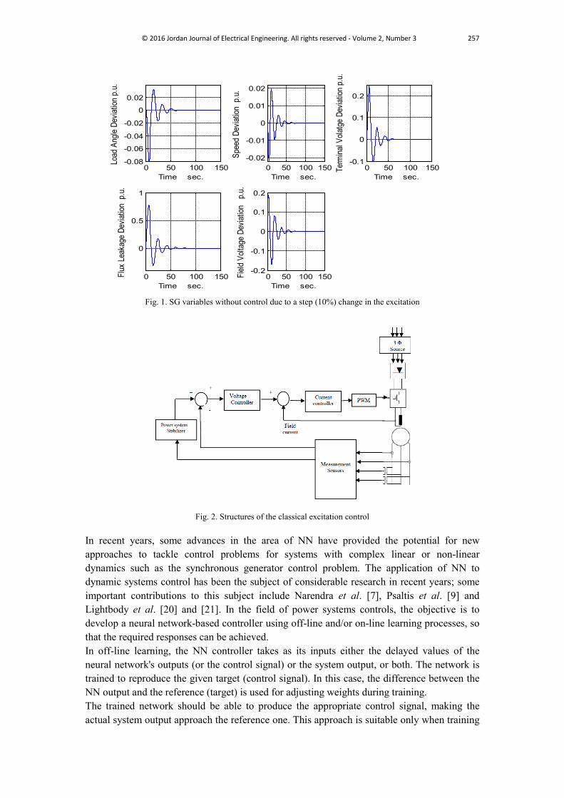
Equation (10) shows the final state-space mathematical model obtained. It is a set of nonlinear-coupled first order differential equations. In this work, the system investigated has the parametric and initial values, which are given in Tables A2 and A3. These parametric and initial values adopted from [1] are presented in the Appendix. For simulation purposes, the SG system was simulated in C++ environment using numerical techniques based on the forth order Runge-Kutta method with time step size of 0.05ms. The power system under study is tested for (10%) change in excitation to study the open loop performance (the system without controller). The deviations of output states ( δ∆ , ω∆ , V t

∆ ,

ψ∆ F , and V F∆ ) are oscillated before reaching their steady-state values as shown in Fig. 1

which shows that the system is stable but with significant amount of oscillations in the state variables. These oscillations are not acceptable in power system stability considerations; therefore, the stability of the system needs to be improved.

III. NEURAL NETWORK FOR EXCITATION CONTROL OF SG

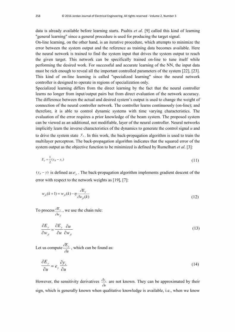
The control of systems having complex, linear or non-linear dynamics using neural network-based methods has become a topic of considerable importance in the research literature. The primary object of any controller is to provide an appropriate control signal to the system, so that a desired output is reached. Much development in designing modern as well as traditional controllers has already occurred; the same is not true for neural network (NN) based solutions. In traditional regulation structures of the excitation control of a synchronous generator, proportional integral derivative (PID) voltage controller is mainly adopted for an excitation current controller. The structure of the classical control system is presented in Fig. 2. In particular, much is currently known about adaptive designs, optimal control systems, and multivariable analysis, but there are very few well established methodologies based on neural reasoning. Therefore, the development of NN-based controllers is still quite lagging behind the more traditional forms of control systems.


Fig. 1. SG variables without control due to a step (10%) change in the excitation

Fig. 2. Structures of the classical excitation control

In recent years, some advances in the area of NN have provided the potential for new approaches to tackle control problems for systems with complex linear or non-linear dynamics such as the synchronous generator control problem. The application of NN to dynamic systems control has been the subject of considerable research in recent years; some important contributions to this subject include Narendra et al. [7], Psaltis et al. [9] and Lightbody et al. [20] and [21]. In the field of power systems controls, the objective is to develop a neural network-based controller using off-line and/or on-line learning processes, so that the required responses can be achieved. In off-line learning, the NN controller takes as its inputs either the delayed values of the neural network's outputs (or the control signal) or the system output, or both. The network is trained to reproduce the given target (control signal). In this case, the difference between the NN output and the reference (target) is used for adjusting weights during training. The trained network should be able to produce the appropriate control signal, making the actual system output approach the reference one. This approach is suitable only when training

0 50 100 150-0.08

-0.06

-0.04

-0.02

0

0.02

Time sec.

Load

Ang

le De

viatio

n p.

u.

0 50 100 150-0.02

-0.01

0

0.01

0.02

Time sec.

Spee

d De

viatio

n p

.u.

0 50 100 150-0.1

0

0.1

0.2

Time sec.

Ter

mina

l Vola

tge

Devia

tion

p.u.

0 50 100 150

0

0.5

1

Time sec.

Flux

Lea

kage

Dev

iation

p.u

.

0 50 100 150-0.2

-0.1

0

0.1

0.2

Time sec.

Field

Volt

age

Devia

tion

p.u

.


data is already available before learning starts. Psaltis et al. [9] called this kind of learning "general learning" since a general procedure is used for producing the target signal. On-line learning, on the other hand, is an iterative procedure, which attempts to minimize the error between the system output and the reference as training data becomes available. Here the neural network is trained to find the system input that drives the system output to reach the given target. This network can be specifically trained on-line to tune itself while performing the desired work. For successful and accurate learning of the NN, the input data must be rich enough to reveal all the important controlled parameters of the system [22], [23]. This kind of on-line learning is called "specialized learning" since the neural network controller is designed to operate in regions of specialization only. Specialized learning differs from the direct learning by the fact that the neural controller learns no longer from input/output pairs but from direct evaluation of the network accuracy. The difference between the actual and desired system’s output is used to change the weight of connection of the neural controller network. The controller learns continuously (on-line); and therefore, it is able to control dynamic systems with time varying characteristics. The evaluation of the error requires a prior knowledge of the beam system. The proposed system can be viewed as an additional, not modifiable, layer of the neural controller. Neural networks implicitly learn the inverse characteristics of the dynamics to generate the control signal u and to drive the system state sy . In this work, the back-propagation algorithm is used to train the multilayer perceptron. The back-propagation algorithm indicates that the squared error of the system output as the objective function to be minimized is defined by Rumelhart et al. [3]:

)(21

sdy yyE −= (11)

)( yyd − is defined as ye . The back-propagation algorithm implements gradient descent of the

error with respect to the network weights as [19], [7]:

)()()1(

kwE

kwkwji

yjiji ∂

∂η−=+

(12) To process

ji

y

wE

∂∂ , we use the chain rule:

∂

∂

∂

∂∂∂

Ew

Eu

uw

y

ji

y

ji=

(13)

Let us computeu

Ey

∂∂

, which can be found as:

∂

∂∂∂

Eu

eyu

yy

s=

(14)

However, the sensitivity derivatives uys

∂∂ are not known. They can be approximated by their

sign, which is generally known when qualitative knowledge is available, i.e., when we know


the orientation in which the control signal influences the outputs of the plants. Therefore, (14) will be written as:

)sign(uye

uE s

yy

∂∂

∂∂

=

(15)

Where u

Ey

∂∂ represents a gradient approximation by sign. Finally, the back-propagated error

jδ , if unit j is an output unit, is given by:

δ∂∂j

s

jy

yu

e= ×sign( ) (16)

For hidden units, we can use the standard rule as:

δ δj j k kjs

o w= − ∑( )1 2

(17) Actually, we evaluate the error jδ using (16) by replacing the partial derivative with its signs.

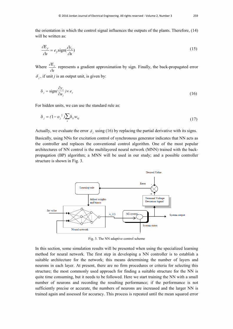
Basically, using NNs for excitation control of synchronous generator indicates that NN acts as the controller and replaces the conventional control algorithm. One of the most popular architectures of NN control is the multilayered neural network (MNN) trained with the back- propagation (BP) algorithm; a MNN will be used in our study; and a possible controller structure is shown in Fig. 3.

Fig. 3. The NN adaptive control scheme

In this section, some simulation results will be presented when using the specialized learning method for neural network. The first step in developing a NN controller is to establish a suitable architecture for the network; this means determining the number of layers and neurons in each layer. At present, there are no firm procedures or criteria for selecting this structure; the most commonly used approach for finding a suitable structure for the NN is quite time consuming, but it needs to be followed. Here we start training the NN with a small number of neurons and recording the resulting performance; if the performance is not sufficiently precise or accurate, the numbers of neurons are increased and the larger NN is trained again and assessed for accuracy. This process is repeated until the mean squared error


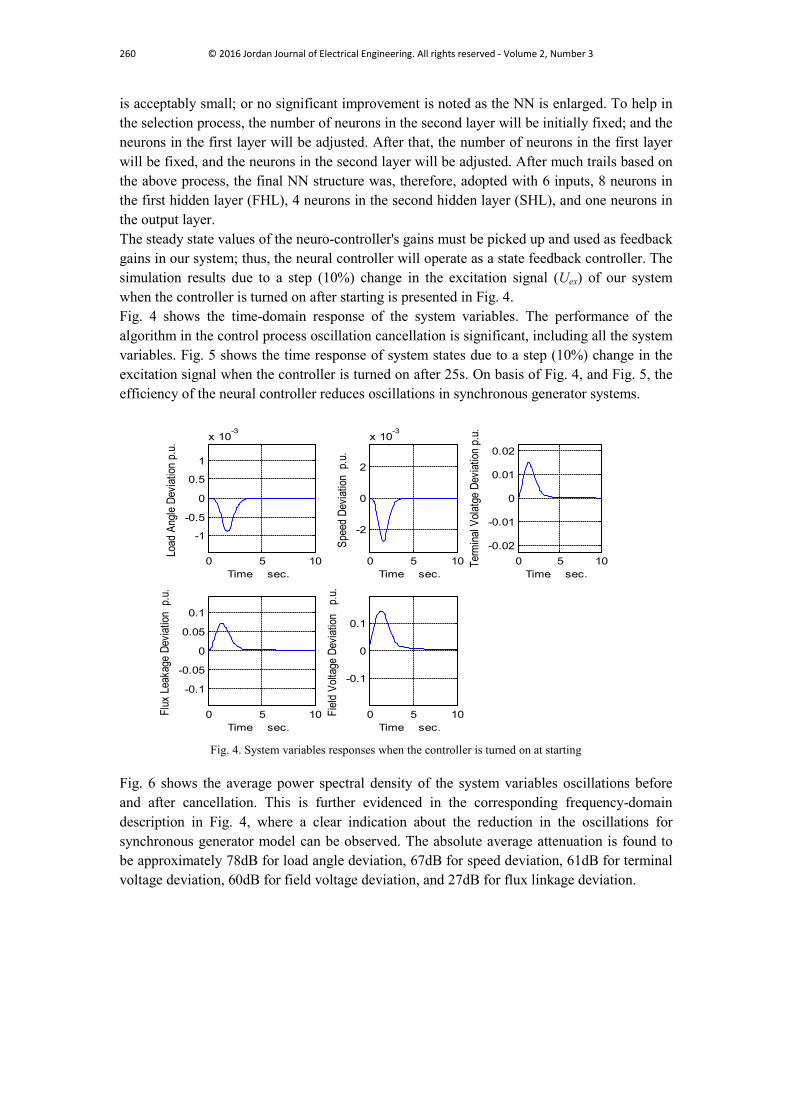
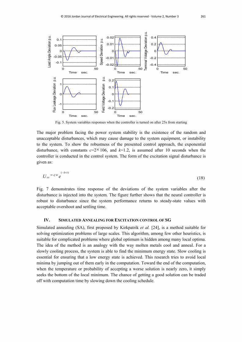
is acceptably small; or no significant improvement is noted as the NN is enlarged. To help in the selection process, the number of neurons in the second layer will be initially fixed; and the neurons in the first layer will be adjusted. After that, the number of neurons in the first layer will be fixed, and the neurons in the second layer will be adjusted. After much trails based on the above process, the final NN structure was, therefore, adopted with 6 inputs, 8 neurons in the first hidden layer (FHL), 4 neurons in the second hidden layer (SHL), and one neurons in the output layer. The steady state values of the neuro-controller's gains must be picked up and used as feedback gains in our system; thus, the neural controller will operate as a state feedback controller. The simulation results due to a step (10%) change in the excitation signal (Uex) of our system when the controller is turned on after starting is presented in Fig. 4. Fig. 4 shows the time-domain response of the system variables. The performance of the algorithm in the control process oscillation cancellation is significant, including all the system variables. Fig. 5 shows the time response of system states due to a step (10%) change in the excitation signal when the controller is turned on after 25s. On basis of Fig. 4, and Fig. 5, the efficiency of the neural controller reduces oscillations in synchronous generator systems.

Fig. 4. System variables responses when the controller is turned on at starting

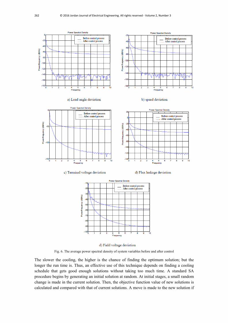
Fig. 6 shows the average power spectral density of the system variables oscillations before and after cancellation. This is further evidenced in the corresponding frequency-domain description in Fig. 4, where a clear indication about the reduction in the oscillations for synchronous generator model can be observed. The absolute average attenuation is found to be approximately 78dB for load angle deviation, 67dB for speed deviation, 61dB for terminal voltage deviation, 60dB for field voltage deviation, and 27dB for flux linkage deviation.

0 5 10

-1

-0.5

0

0.5

1

x 10-3

Time sec.

Load

Ang

le De

viatio

n p.

u.

0 5 10

-2

0

2

x 10-3

Time sec.

Spee

d De

viatio

n p

.u.

0 5 10-0.02

-0.01

0

0.01

0.02

Time sec.

Ter

mina

l Vola

tge

Devia

tion

p.u.

0 5 10

-0.1

-0.05

0

0.05

0.1

Time sec.

Flux

Lea

kage

Dev

iation

p.u

.

0 5 10

-0.1

0

0.1

Time sec.

Field

Volt

age

Devia

tion

p.u

.


Fig. 5. System variables responses when the controller is turned on after 25s from starting

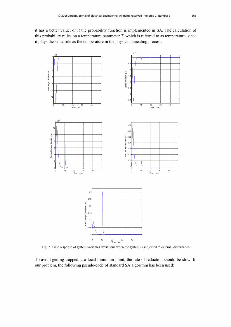
The major problem facing the power system stability is the existence of the random and unacceptable disturbances, which may cause damage to the system equipment, or instability to the system. To show the robustness of the presented control approach, the exponential disturbance, with constants c=2×106, and k=1.2, is assumed after 10 seconds when the controller is conducted in the control system. The form of the excitation signal disturbance is given as:

eUtk

exc

)( ×−×=

(18) Fig. 7 demonstrates time response of the deviations of the system variables after the disturbance is injected into the system. The figure further shows that the neural controller is robust to disturbance since the system performance returns to steady-state values with acceptable overshoot and settling time.

IV. SIMULATED ANNEALING FOR EXCITATION CONTROL OF SG

Simulated annealing (SA), first proposed by Kirkpatrik et al. [24], is a method suitable for solving optimization problems of large scales. This algorithm, among few other heuristics, is suitable for complicated problems where global optimum is hidden among many local optima. The idea of the method is an analogy with the way molten metals cool and anneal. For a slowly cooling process, the system is able to find the minimum energy state. Slow cooling is essential for ensuring that a low energy state is achieved. This research tries to avoid local minima by jumping out of them early in the computation. Toward the end of the computation, when the temperature or probability of accepting a worse solution is nearly zero, it simply seeks the bottom of the local minimum. The chance of getting a good solution can be traded off with computation time by slowing down the cooling schedule.

0 50

-0.1

-0.05

0

0.05

0.1

Time sec.

Load

Ang

le De

viatio

n p.u.

0 50-0.02

-0.01

0

0.01

0.02

Time sec.

Spee

d Dev

iation

p.u.

0 50-0.4

-0.2

0

0.2

0.4

Time sec.

Term

inal V

olatge

Dev

iation

p.u.

0 50

-1

0

1

Time sec.

Flux L

eaka

ge D

eviat

ion p

.u.

0 50-0.2

-0.1

0

0.1

0.2

Time sec.

Field

Volta

ge D

eviat

ion

p.u.


Fig. 6. The average power spectral density of system variables before and after control

The slower the cooling, the higher is the chance of finding the optimum solution; but the longer the run time is. Thus, an effective use of this technique depends on finding a cooling schedule that gets good enough solutions without taking too much time. A standard SA procedure begins by generating an initial solution at random. At initial stages, a small random change is made in the current solution. Then, the objective function value of new solutions is calculated and compared with that of current solutions. A move is made to the new solution if


it has a better value; or if the probability function is implemented in SA. The calculation of this probability relies on a temperature parameter T, which is referred to as temperature, since it plays the same role as the temperature in the physical annealing process.

Fig. 7. Time response of system variables deviations when the system is subjected to external disturbance

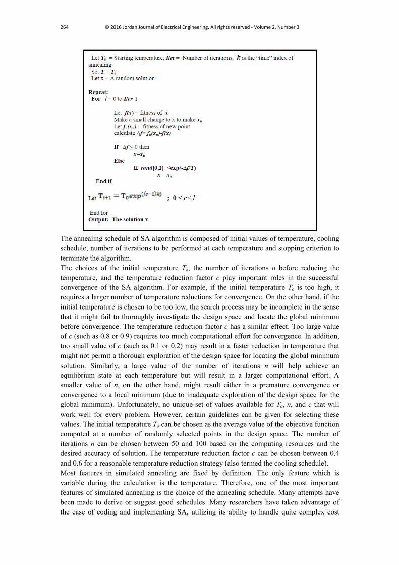
To avoid getting trapped at a local minimum point, the rate of reduction should be slow. In our problem, the following pseudo-code of standard SA algorithm has been used:

0 10 20 30 40

-12

-10

-8

-6

-4

-2

0x 10

-4

Time sec.

Load

Ang

le D

evia

tion

p.u.

0 10 20 30 40

-3.5

-3

-2.5

-2

-1.5

-1

-0.5

0

x 10-3

Time sec.

Spe

ed D

evia

tion

p.u

.

0 10 20 30 400

2

4

6

8

10

12

x 10-3

Time sec.

Ter

min

al V

olat

ge D

evia

tion

p.u.

0 10 20 30 40

0

0.01

0.02

0.03

0.04

0.05

0.06

0.07

Time sec.

Flux

Lea

kage

Dev

iatio

n p

.u.

0 10 20 30 40

0

0.05

0.1

0.15

0.2

0.25

0.3

Time sec.

Fiel

d V

olta

ge D

evia

tion

p.u

.


The annealing schedule of SA algorithm is composed of initial values of temperature, cooling schedule, number of iterations to be performed at each temperature and stopping criterion to terminate the algorithm. The choices of the initial temperature To, the number of iterations n before reducing the temperature, and the temperature reduction factor c play important roles in the successful convergence of the SA algorithm. For example, if the initial temperature To is too high, it requires a larger number of temperature reductions for convergence. On the other hand, if the initial temperature is chosen to be too low, the search process may be incomplete in the sense that it might fail to thoroughly investigate the design space and locate the global minimum before convergence. The temperature reduction factor c has a similar effect. Too large value of c (such as 0.8 or 0.9) requires too much computational effort for convergence. In addition, too small value of c (such as 0.1 or 0.2) may result in a faster reduction in temperature that might not permit a thorough exploration of the design space for locating the global minimum solution. Similarly, a large value of the number of iterations n will help achieve an equilibrium state at each temperature but will result in a larger computational effort. A smaller value of n, on the other hand, might result either in a premature convergence or convergence to a local minimum (due to inadequate exploration of the design space for the global minimum). Unfortunately, no unique set of values available for To, n, and c that will work well for every problem. However, certain guidelines can be given for selecting these values. The initial temperature To can be chosen as the average value of the objective function computed at a number of randomly selected points in the design space. The number of iterations n can be chosen between 50 and 100 based on the computing resources and the desired accuracy of solution. The temperature reduction factor c can be chosen between 0.4 and 0.6 for a reasonable temperature reduction strategy (also termed the cooling schedule). Most features in simulated annealing are fixed by definition. The only feature which is variable during the calculation is the temperature. Therefore, one of the most important features of simulated annealing is the choice of the annealing schedule. Many attempts have been made to derive or suggest good schedules. Many researchers have taken advantage of the ease of coding and implementing SA, utilizing its ability to handle quite complex cost


functions and constraints. However, the long time of execution of standard Boltzmann-type SA has driven these projects to utilize a temperature schedule and satisfy the sufficiency conditions required to establish a true search. Our annealing procedure involves ‘melting’ the system at a high temperature, before repeatedly lowering the temperature by a factor using the Boltzmann algorithm, which is an exponential schedule form:

))1((1 exp kc

oi TT −+ = (19)

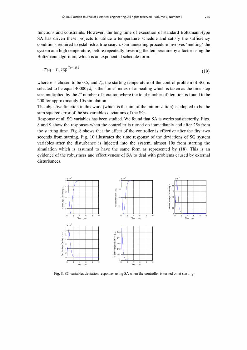
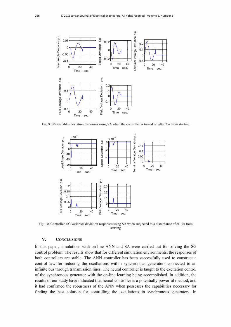
where c is chosen to be 0.5; and To, the starting temperature of the control problem of SG, is selected to be equal 40000; ki is the "time" index of annealing which is taken as the time step size multiplied by the ith number of iteration where the total number of iteration is found to be 200 for approximately 10s simulation. The objective function in this work (which is the aim of the minimization) is adopted to be the sum squared error of the six variables deviations of the SG. Response of all SG variables has been studied. We found that SA is works satisfactorily. Figs. 8 and 9 show the responses when the controller is turned on immediately and after 25s from the starting time. Fig. 8 shows that the effect of the controller is effective after the first two seconds from starting. Fig. 10 illustrates the time response of the deviations of SG system variables after the disturbance is injected into the system, almost 10s from starting the simulation which is assumed to have the same form as represented by (18). This is an evidence of the robustness and effectiveness of SA to deal with problems caused by external disturbances.

Fig. 8. SG variables deviation responses using SA when the controller is turned on at starting

0 2 4 6 8 10

-5

-4

-3

-2

-1

0x 10

-5

Time sec.

Load

Ang

le D

evia

tion

p.u.

0 2 4 6 8 10

-15

-10

-5

0x 10

-5

Time sec.

Spe

ed D

evia

tion

p.u

.

0 2 4 6 8 100

0.5

1

1.5

2

2.5

x 10-3

Time sec.

Ter

min

al V

olat

ge D

evia

tion

p.u.

0 2 4 6 8 10

0

2

4

6

8

10

12

x 10-3

Time sec.

Flux

Lea

kage

Dev

iatio

n p

.u.

0 2 4 6 8 100

0.01

0.02

0.03

0.04

0.05

Time sec.

Fiel

d V

olta

ge D

evia

tion

p.u

.


Fig. 9. SG variables deviation responses using SA when the controller is turned on after 25s from starting

Fig. 10. Controlled SG variables deviation responses using SA when subjected to a disturbance after 10s from

starting

V. CONCLUSIONS

In this paper, simulations with on-line ANN and SA were carried out for solving the SG control problem. The results show that for different simulation environments, the responses of both controllers are stable. The ANN controller has been successfully used to construct a control law for reducing the oscillations within synchronous generators connected to an infinite bus through transmission lines. The neural controller is taught to the excitation control of the synchronous generator with the on-line learning being accomplished. In addition, the results of our study have indicated that neural controller is a potentially powerful method; and it had confirmed the robustness of the ANN when possesses the capabilities necessary for finding the best solution for controlling the oscillations in synchronous generators. In

0 20 40

-0.1

-0.05

0

0.05

Time sec.

Load

Ang

le D

evia

tion

p.u.

0 20 40

-0.02

0

0.02

Time sec.

Spe

ed D

evia

tion

p.u

.

0 20 40-0.1

0

0.1

0.2

Time sec.

Ter

min

al V

olat

ge D

evia

tion

p.u.

0 20 40-0.5

0

0.5

Time sec. Flux

Lea

kage

Dev

iatio

n p

.u.

0 20 40

-0.1

0

0.1

0.2

Time sec. Fiel

d V

olta

ge D

evia

tion

p.u

.

0 20 40-20

-15

-10

-5

0

x 10-4

Time sec.

Load

Ang

le D

evia

tion

p.u.

0 20 40

-4

-2

0x 10

-3

Time sec.

Spe

ed D

evia

tion

p.u

.

0 20 400

0.05

0.1

0.15

Time sec.

Ter

min

al V

olat

ge D

evia

tion

p.u.

0 20 400

0.05

0.1

0.15

0.2

Time sec. Flux

Lea

kage

Dev

iatio

n p

.u.

0 20 40

0

0.1

0.2

0.3

Time sec. Fiel

d V

olta

ge D

evia

tion

p.u

.


addition, the potential of this controller was demonstrated through conducting the control process form starting and after a certain period of time. It demonstrated an excellent control action within the first three seconds. The SA controller was found to be an effective approach for solving this problem. It is relatively easy to comprehend because it is intuitive and involves only simple function of evaluations compared to the NN controller. The results obtained in this case show how quickly they respond and damp out oscillations in all SG system variables. The system reaches its steady state in about two seconds while the NN controller needs about 3s to accomplish the problem of cancellations. Like NN, SA gives the quality of the final solution that is not affected by the initial guesses, except that the computational effort may increase with worse starting designs. In addition, because of the discrete nature of the functional and constraint evaluations, the convergence or transition characteristics are not affected by the continuity or differentiability of the functions. Actually, one of the major problems faced when using this kind of solution is its enormous computational demands. Because the on-line ANN and SA should work during all the period, the execution time is more quite high. Here, SA controller implementation in the control process needs less execution time than that obtained for using ANN. Therefore, it was faster in dealing with the cancellation of oscillation as the results indicate. For applying such on-line controllers on real-time applications, more than one processor needs to be considered. The adaptation of parallel computing techniques to achieve real-time performances would be useful; and such implementation is left for future work. In view of the simulation results obtained, it can be concluded with some confidence that the ANN and SA control strategies offer a viable solution for excitation control of SG problems. APPENDIX

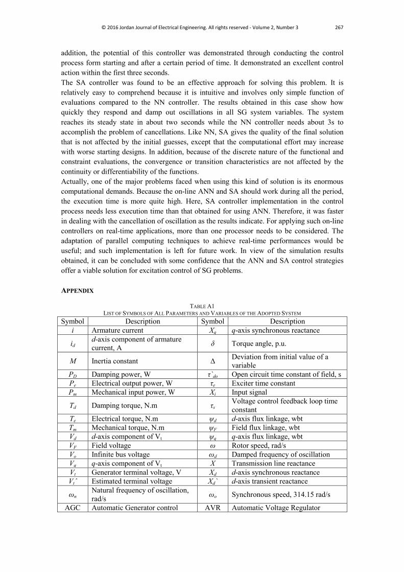
TABLE A1 LIST OF SYMBOLS OF ALL PARAMETERS AND VARIABLES OF THE ADOPTED SYSTEM

Symbol Description Symbol Description i Armature current Xq q-axis synchronous reactance

id d-axis component of armature current, A δ Torque angle, p.u.

M Inertia constant Δ Deviation from initial value of a variable

PD Damping power, W τ`do Open circuit time constant of field, s Pe Electrical output power, W τe Exciter time constant Pm Mechanical input power, W Xi Input signal

Td Damping torque, N.m τs Voltage control feedback loop time constant

Te Electrical torque, N.m ψd d-axis flux linkage, wbt Tm Mechanical torque, N.m ψF Field flux linkage, wbt Vd d-axis component of Vt ψq q-axis flux linkage, wbt VF Field voltage ω Rotor speed, rad/s Vo Infinite bus voltage ωd Damped frequency of oscillation Vq q-axis component of Vt X Transmission line reactance Vt Generator terminal voltage, V Xd d-axis synchronous reactance Vtˆ Estimated terminal voltage Xd` d-axis transient reactance

ωn Natural frequency of oscillation, rad/s ωo Synchronous speed, 314.15 rad/s

AGC Automatic Generator control AVR Automatic Voltage Regulator


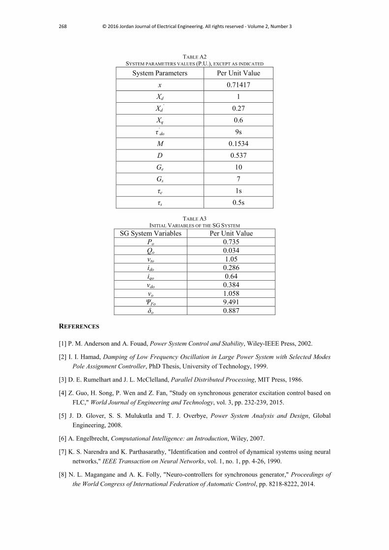
TABLE A2

SYSTEM PARAMETERS VALUES (P.U.), EXCEPT AS INDICATED

System Parameters Per Unit Value x 0.71417 Xd 1 Xd

’ 0.27 Xq 0.6 τ`do 9s M 0.1534 D 0.537 Ge 10 Gs 7 τe 1s τs 0.5s

TABLE A3

INITIAL VARIABLES OF THE SG SYSTEM SG System Variables Per Unit Value

Po 0.735 Qo 0.034 vto 1.05 ido 0.286 iqo 0.64 vdo 0.384 vo 1.058 ΨFo 9.491 δo 0.887

REFERENCES

[1] P. M. Anderson and A. Fouad, Power System Control and Stability, Wiley-IEEE Press, 2002.

[2] I. I. Hamad, Damping of Low Frequency Oscillation in Large Power System with Selected Modes Pole Assignment Controller, PhD Thesis, University of Technology, 1999.

[3] D. E. Rumelhart and J. L. McClelland, Parallel Distributed Processing, MIT Press, 1986.

[4] Z. Guo, H. Song, P. Wen and Z. Fan, "Study on synchronous generator excitation control based on FLC," World Journal of Engineering and Technology, vol. 3, pp. 232-239, 2015.

[5] J. D. Glover, S. S. Mulukutla and T. J. Overbye, Power System Analysis and Design, Global Engineering, 2008.

[6] A. Engelbrecht, Computational Intelligence: an Introduction, Wiley, 2007.

[7] K. S. Narendra and K. Parthasarathy, "Identification and control of dynamical systems using neural networks," IEEE Transaction on Neural Networks, vol. 1, no. 1, pp. 4-26, 1990.

[8] N. L. Magangane and A. K. Folly, "Neuro-controllers for synchronous generator," Proceedings of the World Congress of International Federation of Automatic Control, pp. 8218-8222, 2014.


[9] D. Psaltis, A. Sideris and A. Yamamura, "Neural controllers," Proceedings of IEEE First International Conference on Neural Networks, pp. 551-558, 1987.

[10] L. Wolf and A. Shashua, "Feature selection for unsupervised and supervised inference: the emergence of sparsely in a weight-based approach," Journal of Machine Learning Research, vol. 6, pp. 1855-1887, 2005.

[11] J. A. Starzyk, Z. Zhu and T. Liu, "A self-organizing learning array," IEEE Transactions on Neural Networks, vol. 16, no. 2, pp. 382-289, 2005.

[12] H. He and J. A. Starzyk, "A self-organizing learning array system for power quality classification based on wavelet transform," IEEE Transactions on Power Electronics, vol. 25, no. 2, pp. 382-289, 2010.

[13] T. Fukuda and S. Takanori, "Theory and applications of neural networks for industrial control systems," IEEE Transactions on Industrial Electronics, vol. 39, no. 6, pp. 472-486, 1992.

[14] S. Cong and y. Liang, "PID-like neural network nonlinear adaptive control for uncertain multivariable motion control systems," IEEE Transactions on Industrial Electronics, vol. 56, no. 10, pp. 3872-3879, 2009.

[15] N. Bulic and E. Krasse, "Neural network based excitation control of synchronous generator," Proceedings of The International Conference on Computer as a Tool, pp. 1935-1941, 2007.

[16] N. B. Karayiannis and A. N. Venetsanopoulos, Artificial Networks: Learning Algorithms, Performance Evaluation, and Applications, Springer, 1993.

[17] M. M. Salem, O. P. Malik, A. M. Zaki, O. A. Mahgoub and A. E. El-Zahab, "Simple neuro-controller with modified error function for a synchronous generator," Electrical Power and Energy Systems, vol. 25, no. 9, pp. 759-771, 2003.

[18] A. F. Bati, "On-line computer control of synchronous generator using state estimation and state feedback with particular reference to the excitation system," Engineering and Technology, vol. 11, no. A2, pp. 24-33, 1992.

[19] Y. Yao, Power System Dynamic, Academic Press, 1983.

[20] G. Lightbody and G. W. Irwin, "Nonlinear control structures based on embedded neural system models," IEEE Transactions on Neural Networks, vol. 8, no. 3, pp. 553-567, 1997.

[21] G. Lightbody and G. W. Irwin, "Direct neural model reference adaptive control," IEE Proceeding on Control Theory and Application, pp. 31-43, 1995.

[22] G. K. Venayagamoorthy and R. G. Harley, "Two separate continually online-trained neurocontrollers for excitation and turbine control of a turbo-generator," IEEE Transactions on Industry Applications, vol. 38, no. 3, pp. 887-893, 2002.

[23] J. Ghaboussi and A. Joghataie, "Active control of structures using neural networks," Engineering Mechanics, vol. 121, no. 4, pp. 555-567, 1995.

[24] S. Kirkpatrik, C. D. Gelatt and M. P. Vecchi, "Optimization by simulated annealing," IBM Research Report RC 9355, 1982.

http://ieeexplore.ieee.org/search/searchresult.jsp?searchWithin=%22Authors%22:.QT.G.%20K.%20Venayagamoorthy.QT.&newsearch=true

http://ieeexplore.ieee.org/search/searchresult.jsp?searchWithin=%22Authors%22:.QT.R.%20G.%20Harley.QT.&newsearch=true

jjee pages 253-269 jordan journal of electrical

Documents