J.M. Prusa1 and W.J. Gutowski2

1Teraflux Corporation, Boca Raton, FL; jprusa@bellsouth.net2Iowa State University, Ames, IA; gutowski@iastate.edu

Multi-scale Waves in Sound-Proof Global Simulations with EULAG

3rd International EULAG Workshop, Loughborough, UK

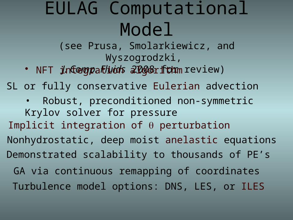
EULAG Computational Model(see Prusa, Smolarkiewicz, and Wyszogrodzki,

J. Comp. Fluids 2008 for review)

• NFT integration algorithm

• SL or fully conservative Eulerian advection

• Robust, preconditioned non-symmetric Krylov solver for pressure

• Implicit integration of perturbation

• Nonhydrostatic, deep moist anelastic equations

• Demonstrated scalability to thousands of PE’s

• GA via continuous remapping of coordinates

• Turbulence model options: DNS, LES, or ILES

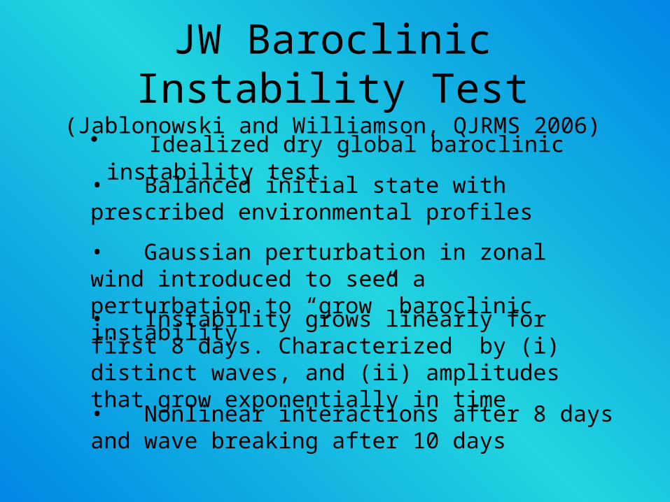
JW Baroclinic Instability Test(Jablonowski and Williamson, QJRMS 2006)

• Idealized dry global baroclinic instability test

• Balanced initial state with prescribed environmental profiles

• Gaussian perturbation in zonal wind introduced to seed a perturbation to “grow” baroclinic instability

• Instability grows linearly for first 8 days. Characterized by (i) distinct waves, and (ii) amplitudes that grow exponentially in time

• Nonlinear interactions after 8 days and wave breaking after 10 days

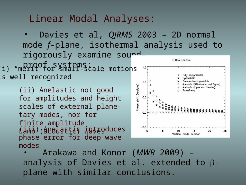
Linear Modal Analyses:

• Davies et al, QJRMS 2003 – 2D normal mode f-plane, isothermal analysis used to rigorously examine sound-proof systems:

(ii) Anelastic not good for amplitudes and height scales of external plane-tary modes, nor for finite amplitude Lamb (acoustic) waves

(iii) Anelastic introduces phase error for deep wave modes

• Arakawa and Konor (MWR 2009) – analysis of Davies et al. extended to -plane with similar conclusions.

(i) “merit for small-scale motionsis well recognized”

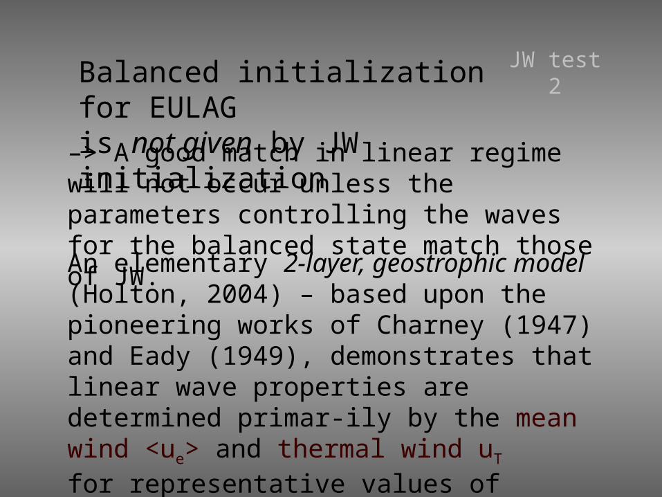
JW test 2

–> A good match in linear regime will not occur unless the parameters controlling the waves for the balanced state match those of JW.

Balanced initialization for EULAG is not given by JW initialization

An elementary 2-layer, geostrophic model (Holton, 2004) – based upon the pioneering works of Charney (1947) and Eady (1949), demonstrates that linear wave properties are determined primar-ily by the mean wind <ue> and thermal wind uT for representative values of static stability .

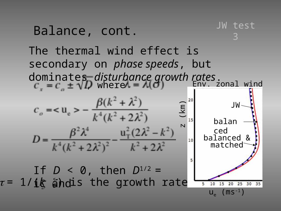
JW test 3Balance, cont.

The thermal wind effect is secondary on phase speeds, but dominates disturbance growth rates.

, where

If D < 0, then D1/2 = i and = 1/(k ) is the growth rate

ue (ms-1)z

(km

)

Env. zonal wind

JW

balanced

balanced &matched

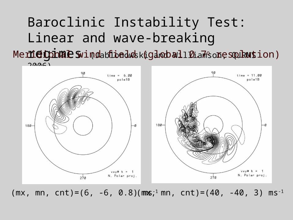
Baroclinic Instability Test: Linear and wave-breaking regimes (Jablonowski and Williamson, QJRMS 2006)

Meridional wind field (global 0.7o resolution)

(mx, mn, cnt)=(6, -6, 0.8) ms-1 (mx, mn, cnt)=(40, -40, 3) ms-1

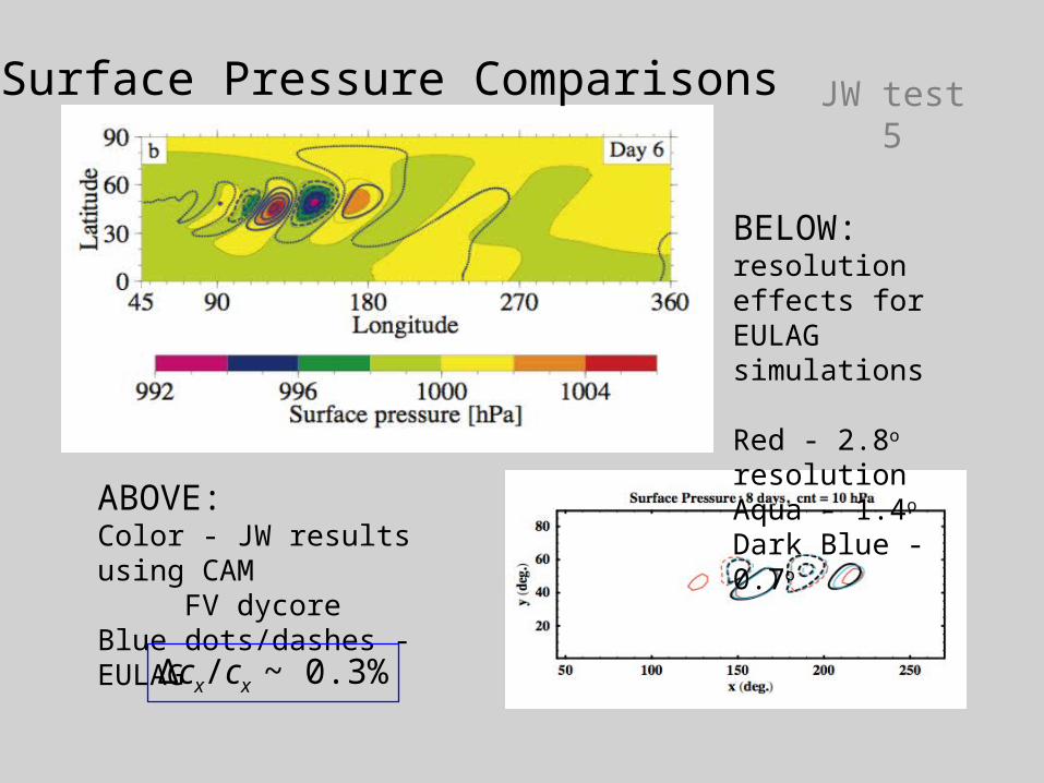
JW test 5

ABOVE:Color - JW results using CAM FV dycoreBlue dots/dashes - EULAG

BELOW:resolution effects for EULAG simulations

Red - 2.8o resolutionAqua - 1.4o

Dark Blue - 0.7o

Surface Pressure Comparisons

Δcx/cx ~ 0.3%

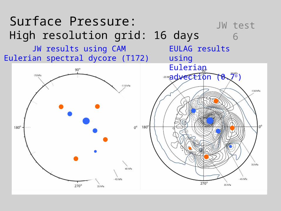
JW test 6

JW results using CAMEulerian spectral dycore (T172)

EULAG results using Eulerian advection (0.7o)

Surface Pressure:High resolution grid: 16 days

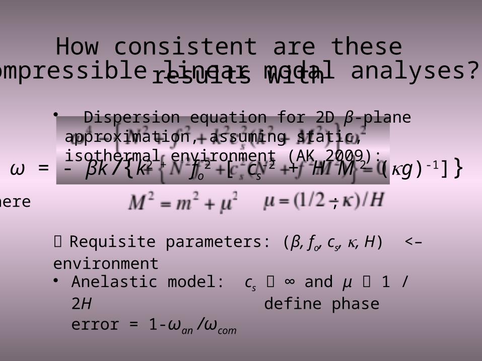
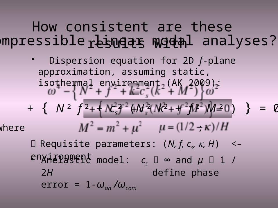
How consistent are these results withcompressible linear modal analyses?

Requisite parameters: (β, fo, cs, , H) <– environment

Anelastic model: cs ∞ and μ 1 / 2H

define phase error = 1-ωan /ωcom

where ;

ω = - βk /{k2 + fo2 [ cs

-2 + H M 2 (g)-1]}

• Dispersion equation for 2D β-plane approximation, assuming static, isothermal environment (AK 2009):

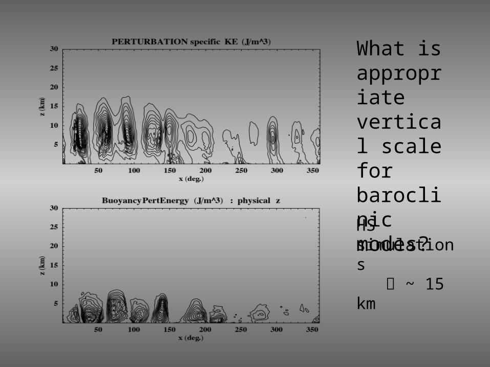
What is appropriate vertical scale for baroclinic modes?

HS simulations ~ 15 km

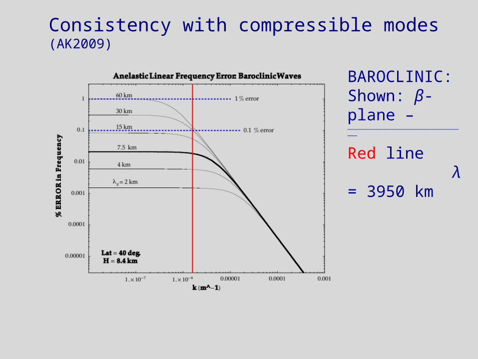
Consistency with compressible modes (AK2009)

BAROCLINIC: Shown: β-plane –______________________________________

Red line λ = 3950 km

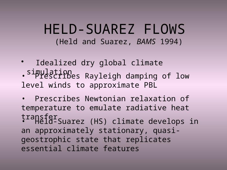
HELD-SUAREZ FLOWS(Held and Suarez, BAMS 1994)

• Idealized dry global climate simulation

• Prescribes Rayleigh damping of low level winds to approximate PBL

• Prescribes Newtonian relaxation of temperature to emulate radiative heat transfer

• Held-Suarez (HS) climate develops in an approximately stationary, quasi-geostrophic state that replicates essential climate features

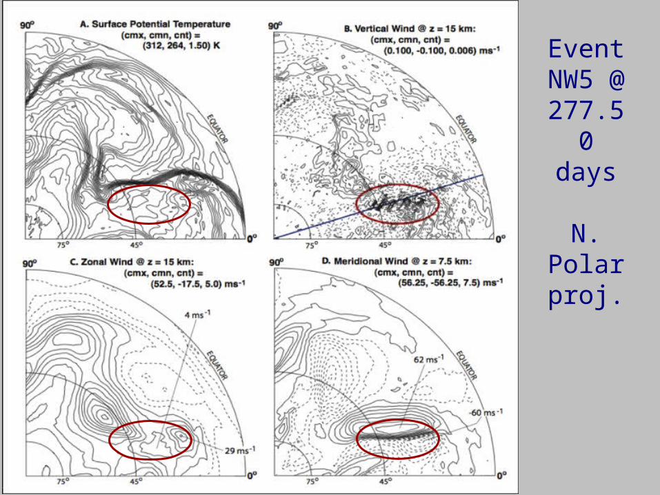
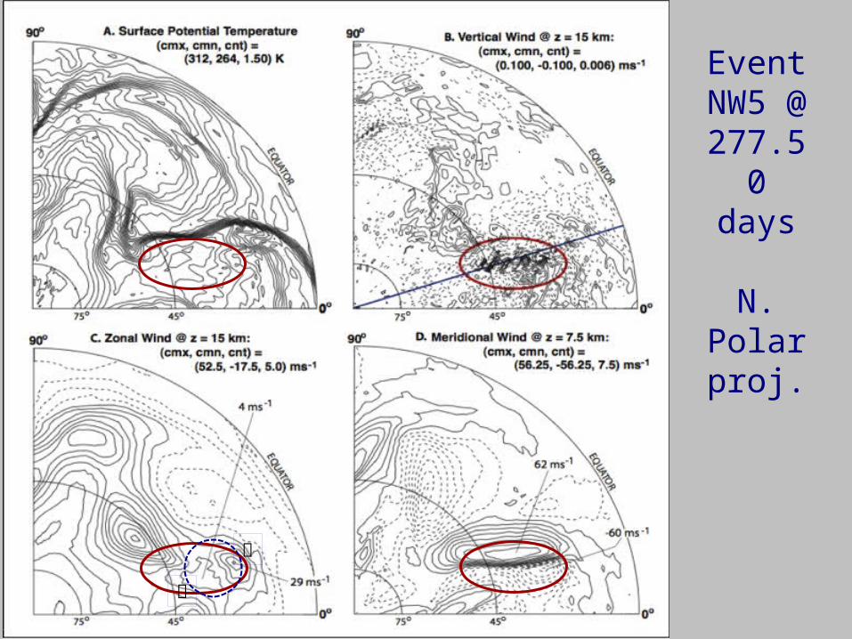
NW5: yz slicesEvent

NW5 @ 277.50 days

N. Polar proj.

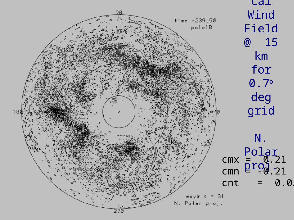
Vertical Wind

Field @ 15 km for 0.7o deg grid

N. Polar proj.

cmx = 0.21cmn = -0.21cnt = 0.02

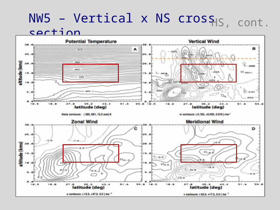
NW5 – Vertical x NS cross section meridional slice @ 18 deg. Long.

HS, cont.

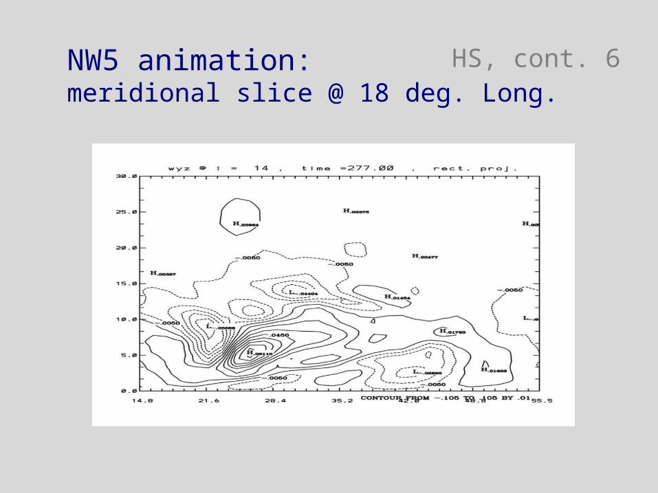
NW5 animation: meridional slice @ 18 deg. Long.

HS, cont. 6

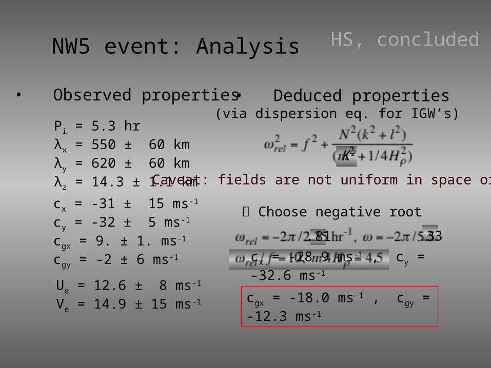
NW5 event: Analysis HS, concluded

• Observed properties

Ue = 12.6 ± 8 ms-1

Ve = 14.9 ± 15 ms-1

cx = -31 ± 15 ms-1

cy = -32 ± 5 ms-1

cgx = 9. ± 1. ms-1

cgy = -2 ± 6 ms-1

Pi = 5.3 hrλx = 550 ± 60 kmλy = 620 ± 60 kmλz = 14.3 ± 1.1 km

• Deduced properties(via dispersion eq. for IGW’s)

Caveat: fields are not uniform in space or time

K 2

Choose negative root

.81 .33

cx = -28.9 ms-1 , cy = -32.6 ms-1

cgx = -18.0 ms-1 , cgy = -12.3 ms-1

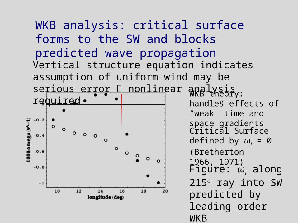
WKB analysis: critical surface forms to the SW and blocks predicted wave propagation

Vertical structure equation indicates assumption of uniform wind may be serious error nonlinear analysis required

Figure: ωi along 215o ray into SW predicted by leading order WKB

WKB theory: handles effects of “weak” time and space gradients

Critical Surface defined by ωi = 0 (Bretherton 1966, 1971)

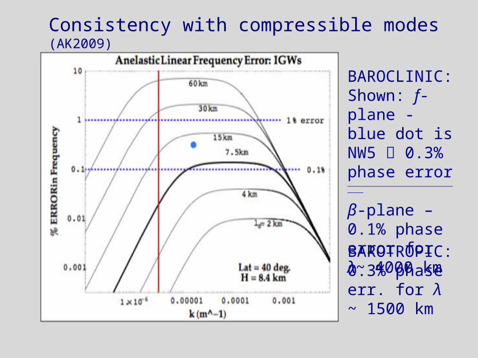
Consistency with compressible modes (AK2009)

BAROCLINIC: Shown: f-plane -blue dot is NW5 0.3% phase error______________________________________

β-plane – 0.1% phase error for λ~ 4000 kmBAROTROPIC: 0.3% phase err. for λ ~ 1500 km

Remarks

• Global HS simulations show (some) localized packets of internal gravity waves in lower stratosphere. Linear modal analysis predicts all properties of a representative wave packet except group velocity, which WKB analysis shows depends strongly upon wind gradients in local environment of waves. Linear analyses do not give correct group velocities due to nonlinear synoptic scale wave interactions.

• Baroclinic wave test results show excellent agreement with published results of JW (2006) in linear wave regime. REQUIRED: initialization balanced for EULAG; andMATCHING of env. mean wind, thermal wind, and stability. In wavebreaking regime, differences arise in details.

Why Baroclinic Motion?• “Baroclinic instability is the most important

form of instability in the atmosphere, as it is responsible for mid-latitude cyclones” (Houghton, 1986)

• Baroclinic wave breaking radiates gravity waves, which act to restore geostrophic balance (Holton, 2004).

Why Study Baroclinic Dynamics?

• “Baroclinic instability is the most important form of instability in the atmosphere, as it is responsible for mid-latitude cyclones” (Houghton, 1986)

• Baroclinic wave breaking radiates gravity waves, which act to restore geostrophic balance (Holton, 2004) –> multi-scale physics

• J. Charney (J. Meteor 1947), E. Eady (Tellus 1949), and J. Smagorinsky (MWR 1963)

• Good test case for multi-scale global atmospheric models• Good test case for multi-scale global atmospheric models

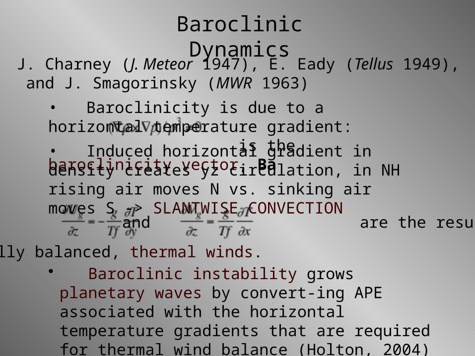
• and are the resulting

geostrophically balanced, thermal winds.

Baroclinic Dynamics

• Baroclinicity is due to a horizontal temperature gradient: is the baroclinicity vector, Ba

• J. Charney (J. Meteor 1947), E. Eady (Tellus 1949), and J. Smagorinsky (MWR 1963)

• Induced horizontal gradient in density creates yz circulation, in NH rising air moves N vs. sinking air moves S -> SLANTWISE CONVECTION

• Baroclinic instability grows planetary waves by convert-ing APE associated with the horizontal temperature gradients that are required for thermal wind balance (Holton, 2004)

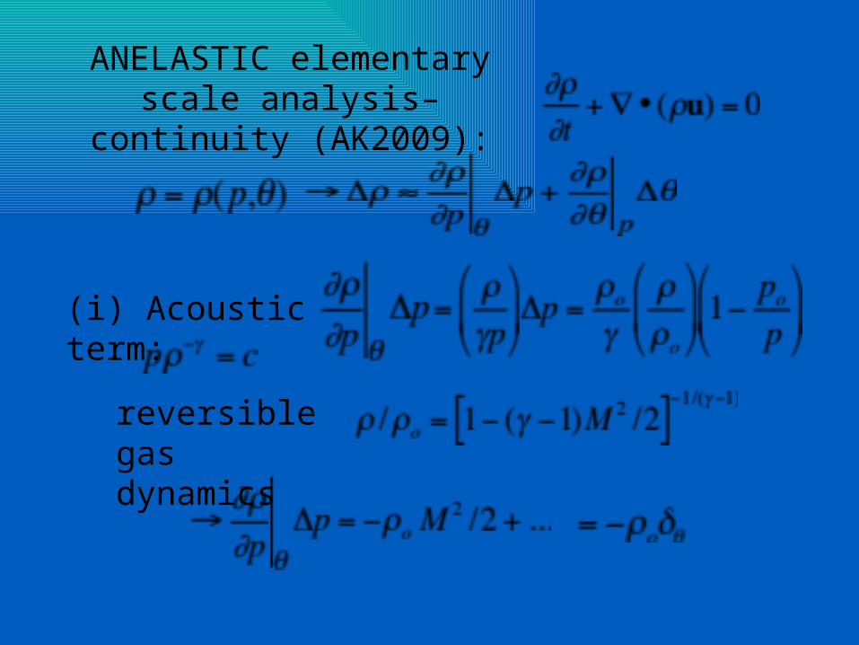
ANELASTIC elementary scale analysis– continuity (AK2009):

(i) Acoustic term:

reversible gas dynamics

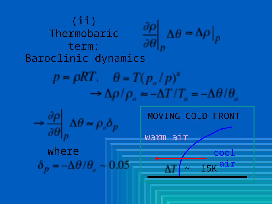
(ii) Thermobaric term:

warm air

cool air ~ 15K

MOVING COLD FRONT

Baroclinic dynamics

where

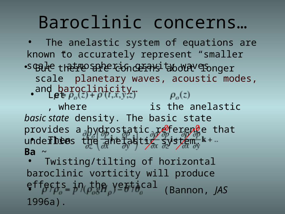
Baroclinic concerns…

• But there are concerns about longer scale planetary waves, acoustic modes, and baroclinicity…

• Then Ba ~

• Let , where is the anelastic basic state density. The basic state provides a hydrostatic reference that underlies the anelastic system.

0 0

• (Bannon, JAS 1996a).

• The anelastic system of equations are known to accurately represent “smaller scale” atmospheric gravity waves

• Twisting/tilting of horizontal baroclinic vorticity will produce effects in the vertical

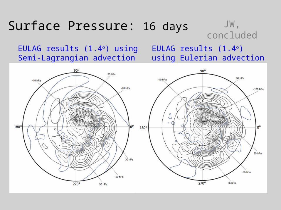
JW, concludedSurface Pressure: 16 days

EULAG results (1.4o)using Eulerian advection

EULAG results (1.4o) using Semi-Lagrangian advection

How consistent are these results with

• Dispersion equation for 2D f-plane approximation, assuming static, isothermal environment (AK 2009):

compressible linear modal analyses?

Requisite parameters: (N, f, cs, , H) <– environment

Anelastic model: cs ∞ and μ 1 / 2H

define phase error = 1-ωan /ωcom

where ;

+ { N 2 f 2 + cs2 (N 2 k2 + f 2 M 2 ) } = 0

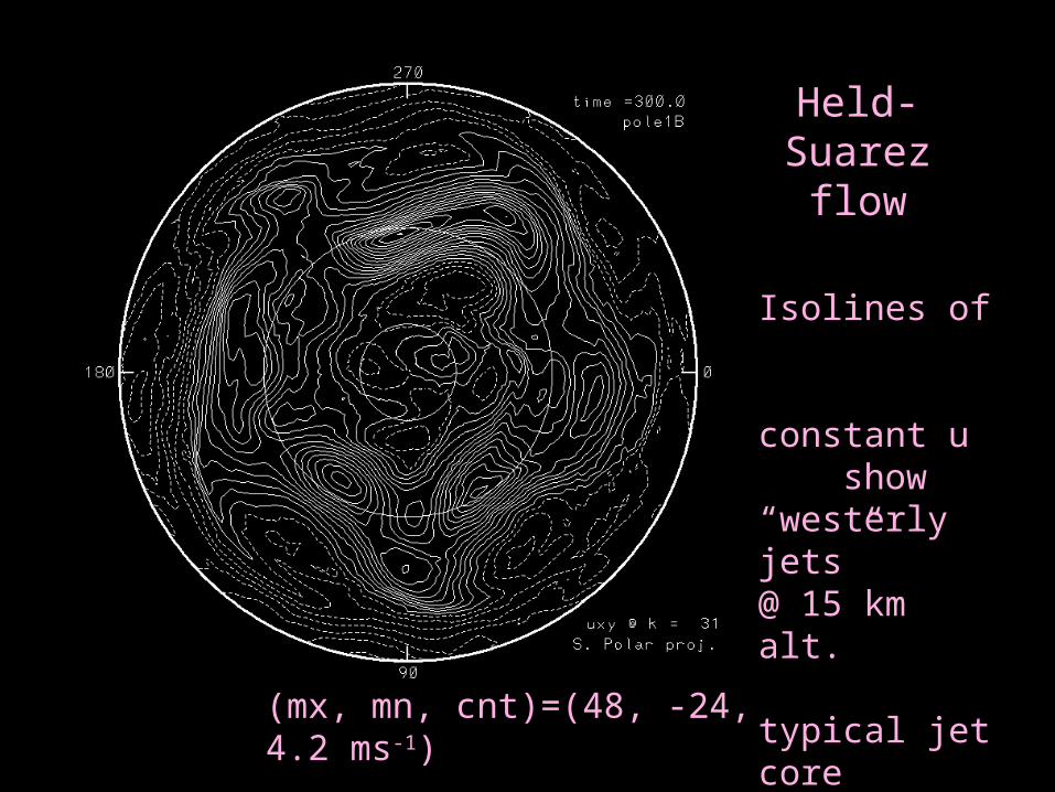
Held-Suarezflow

Isolines of constant u show “westerly jets”@ 15 km alt.

typical jet coreΔ umax ~ 65 ms-1 over synoptic scales

(mx, mn, cnt)=(48, -24, 4.2 ms-1)

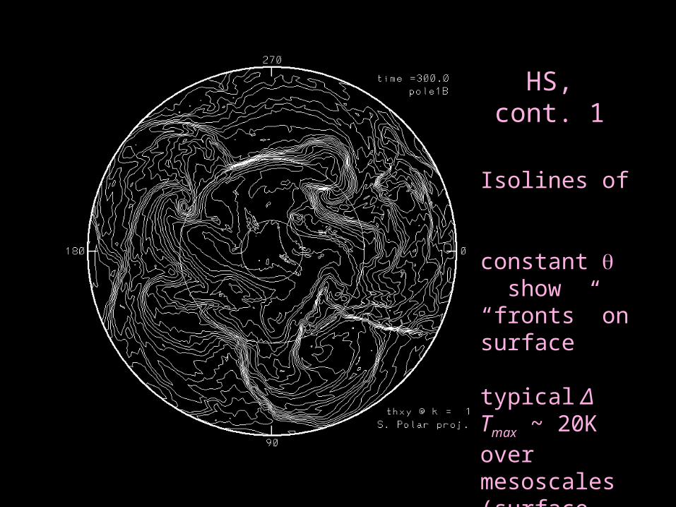
HS, cont. 1

Isolines of constant show “fronts” on surface

typical Δ Tmax ~ 20K over mesoscales (surface fronts)

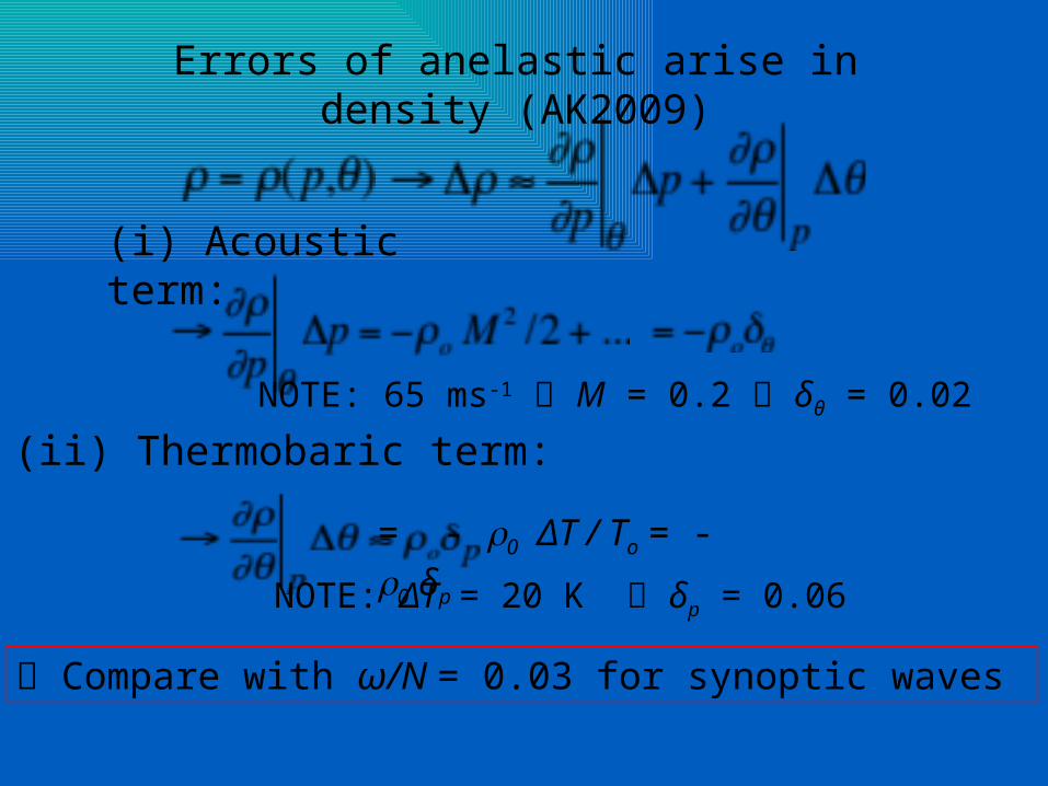
Errors of anelastic arise in density (AK2009)

(i) Acoustic term:

NOTE: 65 ms-1 M = 0.2 δθ = 0.02

Compare with ω/N = 0.03 for synoptic waves

(ii) Thermobaric term:

NOTE: ΔT = 20 K δp = 0.06

= - r0 ΔT / To = - r0 δp

NW5: yz slicesEvent

NW5 @ 277.50 days

N. Polar proj.

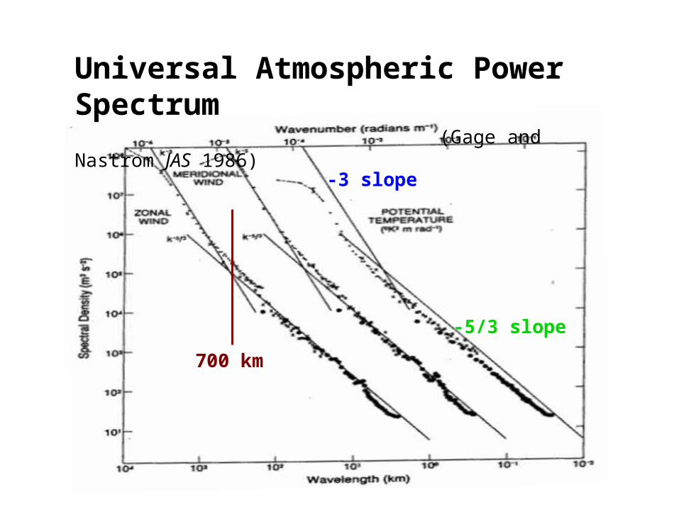
Universal Atmospheric Power Spectrum (Gage and Nastrom JAS 1986)

700 km

-5/3 slope

-3 slope

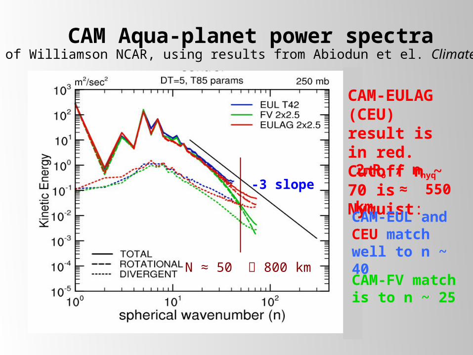
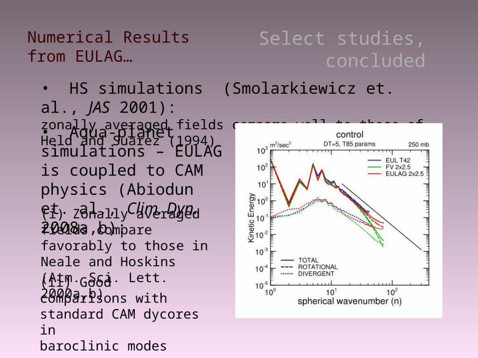
CAM Aqua-planet power spectra(courtesy of Williamson NCAR, using results from Abiodun et el. Climate Dyn. 2008)

N ≈ 50 800 km

2pRo / nnyq

≈ 550 km

CAM-EULAG (CEU) result is in red. Cutoff n ~ 70 is Nyquist:

CAM-FV match is to n ~ 25

CAM-EUL and CEU match well to n ~ 40

-3 slope

Examples

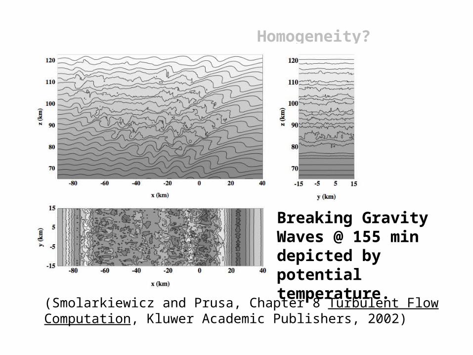
Homogeneity? Isotropy?

Breaking Gravity Waves @ 155 min depicted by potential temperature.

(Smolarkiewicz and Prusa, Chapter 8 Turbulent Flow Computation, Kluwer Academic Publishers, 2002)

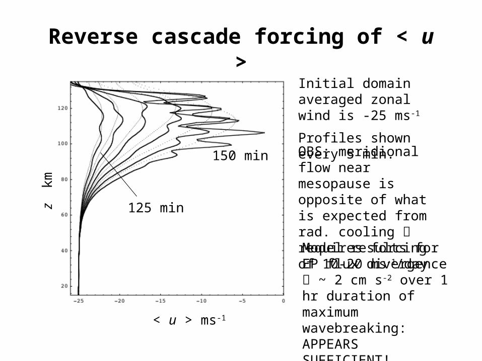
Reverse cascade forcing of < u >

< u > ms-1

z k

m

125 min

150 min

Initial domain averaged zonal wind is -25 ms-1

Profiles shown every 5 min.OBS: meridional flow near mesopause is opposite of what is expected from rad. cooling requires forcing of 10-20 ms-1/day

Model results for EP flux divergence ~ 2 cm s-2 over 1 hr duration of maximum wavebreaking: APPEARS SUFFICIENT!

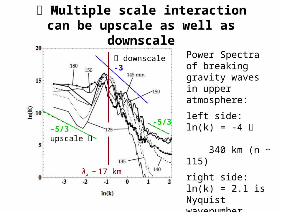
Multiple scale interaction can be upscale as well as downscale

Power Spectra of breaking gravity waves in upper atmosphere:

left side: ln(k) = -4 340 km (n ~ 115)

right side: ln(k) = 2.1 is Nyquist wavenumber λnyq = 760 m

(Prusa et al. Int. J. Math. Comput. Sci. 2001)

λx ~ 17 km

-5/3upscale

-5/3

downscale-3

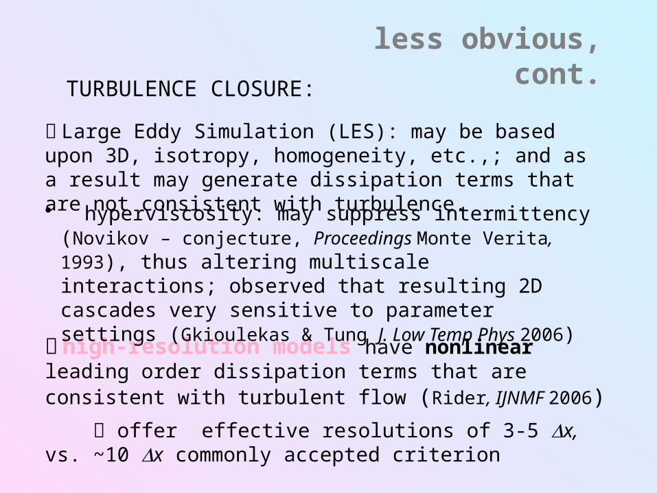
less obvious, cont.

high-resolution models have nonlinear leading order dissipation terms that are consistent with turbulent flow (Rider, IJNMF 2006)

offer effective resolutions of 3-5 Dx, vs. ~10 Dx commonly accepted criterion

Large Eddy Simulation (LES): may be based upon 3D, isotropy, homogeneity, etc.,; and as a result may generate dissipation terms that are not consistent with turbulence.

hyperviscosity: may suppress intermittency (Novikov – conjecture, Proceedings Monte Verita, 1993), thus altering multiscale interactions; observed that resulting 2D cascades very sensitive to parameter settings (Gkioulekas & Tung J. Low Temp Phys 2006)

TURBULENCE CLOSURE:

A Few Select Studies…

• Davies et al, QJRMS 2003 – 2D normal mode f-plane analysis used to rigorously examine sound-proof systems:

(i) Anelastic works well for all gravity wave frequencies

(ii) Anelastic not good for amplitudes and height scales of external planetary modes, nor for finite amplitude Lamb (acoustic) waves

(iii) Anelastic introduces phase error for deep wave modes

• Klein et al., JFM 2010 – multiple parameter, singular perturbation analysis that examines multiscale interaction between planetary and gravity wave modes:

(i) The anelastic sytem “gets it right”, with differences from elastic systems being asymptotically small, of order ~ O( M2/3 )

(ii) This translates into stratification increases of ~ 10% over a pressure scale height

Select studies, concluded

• HS simulations (Smolarkiewicz et. al., JAS 2001):zonally averaged fields compare well to those of Held and Suarez (1994)

Numerical Results from EULAG…

• Aqua-planet simulations – EULAG is coupled to CAM physics (Abiodun et. al., Clim. Dyn. 2008a,b):

(i) Zonally averaged fields compare favorably to those in Neale and Hoskins (Atm. Sci. Lett. 2000a,b)

(ii) Good comparisons with standard CAM dycores in baroclinic modes