John Lyons

CONTENTS

Page

Par_ 1: General Considerations ....................................................................... 1

Background ................................................................................................. 2Structure of"the IBI ....................................................................................... 2Where to Use the IBI ..................................................................................... 3

Using and Interpreting the IB! ..................................................................... 3Accounting for Natural D_erences Among Strea_n Fish CommuF_tles .......... 4

Part 2: Applying the IBI in Wisconsin _Varznwater Streams ............................... 5Collecting and Processing the Field Data ....................................................... 5

Selecting and Delineating Sites for Data Callection ................................... 5Determining When to Sample .................................................................... SDetermining Stream Size ........................................................................... 9Sampling the Fish Community ................................................................... 9Processing the Fish Sample ...................................................................... 9

Analyzing the Data ..................................................................................... I0Determining Stream Location ..................................................................... 10Classifying Fish Species ........................................................................... 10Dealing With Very Low Catch Rates ......................................................... i SUsing MSR Plots tbr Scoring .................................................................... i 8Scoring Metrics Based on Percentages ...... .... ........................................... 22Scoring Correction Factors ........................................................................ 22Calculating the Overall IBI Score ............................................................. 22

Interpreting IBI Scores ................................................................................ 23Interpreting the Overall IBI Score ............................................................. 23Identifying Specific Environmemal Problems ............................................ 23Accounting for Differences Among Samples in IBI Scores ......................... 23Incorporating Other Types of Information. ................................................ 25

Acknowledgments ........................................................................................ 25Literature Cited .............................................................................................. 26

Appendix 1 .............................................................................................. 29Appendix 2 ................................................................................................ 38Appendix 3 .................................................................................................... 41Appendix 4 ........................................... .......................................................... 42Appendix 5 ............................................................................................... 48

North Central Forest Experiment StationForest Service - U.S. Department of Agriculture

1992 Folwell AvenueSt. l_ul, Minnesota 55108

Manuscript approved for publication April 6, 19921992

Using The Index Of Biotic Integrity (IBI) ToMeasttre Environmental Quality In War.water

Strea s of Wisconsirl

John Lyons

PART 1: GENERAL CONSIDERATIONS a pilot study to identify suitable bioassessment/biomonitoring techniques for Wisconsin based

Many varied and complex environmental prob- on fish. The pilot study concluded that antems affect the surface waters of North Amerlca_ existing technique, the Index of Biotic Integrity,To better address some of these problems, a had excellentpotentlal (Forbes and Lyons,new approach to field monitoring and ev_uation WDNR, unpublished data). The Index of Biotichas recently emerged. This approach, generally Integrity, commonly known as the IBI, is atermed "bioassessment _ or "biomonltoring," bioassessment/biomonttoring technique thatuses data on biological populations or commu- allows attributes of fish communities to be usedntties to assess and monitor environmental to assess biotic Integrity and environmental

quality (Plafkln et al. 1989). Bioassessment and quality of streams and rivers {Karr 1981, Karr etblomonitoring techniques have proven valuable a/. 1986).in detecting and quahog many types of envi-ronmental degradation in aquatic systems From 1987 through 1990, my colleagues and I(Berkman and Rabenl 1987, Ohio EPA 1988, from the WDNR collected and analyzed fishFausch et al. 1990, Karr 1991). community data with the aim of developing a

version of the IBI for use In warmwater streams

Although many types of biota have been used in of Wisconsin. This paper summarizes thebioassessment and biomonitoring, benthic results of this effort and presents a detailedmacroinvertebrates and fish have been found to description of how the IBI should be applied and

be particularly effective (Berkman and Rabenl Interpreted in Wisconsin. Because of simflari-1987, Plafkin et al. 1989). Wisconsin pioneered ties in stream characteristics and fish faunathe development of bioassessment and biomonl- between Wisconsin and parts of adjacent States

toting techniques based on benthic macroin- (Page and Burr 1986, Underhill 1986, Omernikvertebrate community data during the 1970's and Gallant 1988), the Wisconsin version of theand early 1980's (Hflsenhoff 1977, 1982). How- IBI described here should also be useful inever, use of fish community data in bioassess- southeastern and northeastern Minnesota, thement/biomonitoring of the State's waters lagged entire Upper Peninsula and the northern Lowerbehind until recently. In 1984, the Wisconsin Peninsula of Michigan, extreme northwesternDepartment of Natural Resources (WDNR) began Illinois, and extreme northeastern Iowa. This

paper is designed primarily as a "how to" man-ual, and as such contains little discussion of

John Lyons is a Fisheries Research Biologist, the underlying principles of the IBI. ReadersFish Research Section, Bureau of Research, interested in a more theoretical treatment of the

Wisconsin Department of Natural Resources, IBI, including a comparison of the IBI with other1350 Feml-ite Drive, Monona, Wisconsin 53716.

environmental indices that are based on fish STRUCTL_E OF THE 1BIcommunities, should refer to Berkman et aL

(i986), Karr et aL (1988), Angermeier and The IBI consists of a series of fish communitySchlosser (1987), Hughes and Gammon (1987), attributes, termed met:dcs_ that reflect basicFausch et al. (1990), Karr (1991), and references structural and functional characteristics of

therein. Appendix 1 describes in more technical biotic assemblages: species richness and corn-detail the data and procedures used to develop position, trophic and reproductive function, andand validate the Wisconsin version, individual abundance and condition. The

number and identity of metrics diker amongBACKGRO_ different versions of the IBI, but all versions

have metrics that measure both structural and

The IBI was originally developed by Dr. James functional characteristics of fish communities.Karr during the late 1970's and early 1980's toassess biotic integrity and environmental qual- The Wisconsin version of the IBI described here

ity in small streams in Indiana and Illinois (Karr consists of 10 basic metrics, plus 2 additional1981, Karr et al. 1986). Karr and Dudley (1981) metrics (termed "correction factors _ later in the

defined biotic integrity as "a balanced, inte- text) that affect the index only when they havegrated, adaptive community of organisms extreme values. These 12 metrics, described inhaving a species composition, diversity, and detail in Part 2, are:functional organization comparable to that of

natural habitat of the region." Although the Species Richness and ComFc:sitionspecific attributes and expectations of the Total number of native speciesoriginal version of the IBI apply only to Indiana Number of darter speciesand Illinois, the general principles underlying Number of sucker speciesthe IBI concept apply to many streams through- Number of sunfish speciesout North America. Karr recognized this, and Number of intolerant specieshe and his colleagues at the University of Illinois Percent (by number of individuals) that aredeveloped procedures for adapting the IBI for tolerant speciesuse in different regions (Fausch et al, 1984,

Karr et al. 1986). Biologists and managers in Trophic and Reproductive Functionother States and Canadian provinces have since Percent that are omntvores

modified the IBI to fit the physical and biological Percent that are insectivorescharacteristics of streams in their areas. They Percent that are top carnivores

have generally found the IBI to be a useful Percent that are simple lithophllous spawnersassessment and evaluation tool (Miller et al.1988, Fausch et al. 1990). Fish Abundance and Condition

Number of individuals (excluding tolerantOne of the most thorough modifications of the species) per 300 m sampledIBI has been done by the Division of Water Percent with deformities, eroded fins, lesions,Quality Monitoring and Assessment of the Ohio or tumors (DELT)Environmental Protection Agency (Ohio EPA

1988). The Ohio EPA developed several versions The last two metrics are not normally includedof the IBI based on hundreds of fish Community, in the calculation of the IBI, but they can lowerhabitat, and water quality samples from a wide the overall IBI score if they have extreme valuesvariety of Ohio streams and rivers. The Ohio (very low number of individuals or high percentEPA uses the IBI extensively, and IBI scores DELT fish).

have been incorporated into Ohio water qualitystandards. The Wisconsin version of the IBI

that I present here is largely derived from theOhio EPA "wading sites" version.

_'_E_ TO USE THE _I USING AND I_'_ERPR_TING THE IBI

The Wisconsin IBI described in this paper is The IBI is calculated for a stream site by corn-appropriate for use only in warmwater it, co, non- paring the observed values of each metric withtrout) streams° Many Wisconsin coldwater values expected in comparable streams of highstreams have too few species for a corpm_unity- environmental quality (Karr et at, 1986). If thelevel index such as the IBt, although the IBI has observed values are close to the expected, thenbeen successfully adapted for trout streams in the stream in question probably has goodthe western U.S. (Miller et at. 1988). More environmental quality. K observed and expectedimportantly, the response of many Wisconsin values are far apart, then the stream is probablycoldwater streams to changes in environmental degraded. Thus, to ca!culate the IBI, it isquality violates one of the key assumptions necessary to know the characteristics of fishunderlying the Wisconsin IBI. 2_e Index is communities in streams of high environmentalpredicated on the assumption that the number quality.of species in a commun_y declines with increas-ing environmental degradation. This assump- In Wisconsin, high quality warmwater streams[ion seems to be valid kn warmwater streams in have many native species, darters, suckers,Wisconsin, but in coldwater streams, the num- sunfish, and intolerant species [species that arebet of species sometimes increases after limited particularly sensitive to water pollution andor moderate degradation. Appendix 2 gives a habitat degradation) (Lyons et al. 1988, Lyonsmore complete analysis of why the Wisconsin 1989). Tolerant species (species capable ofIBI is inappropriate fbr use in coldwater persisting under a wide range of degradedstreams, conditions) are present, but do not dominate.

Most fish are insectivores (species that feed

The Wisconsin tBI is appropriate only for per- primarily on insects or other small macroin-rnanent warmwater streams and rivers of inter- vertebrates), and top carnivores (species thatmediate size. Small headwater or intermittent feed primarily on other vertebrates or largestreams and streams and rivers that are too macrotnvertebrates such as crayfish) are corn-deep or wide to be effectively sampled by wading mon. Omnivores (species that have at least 25require different versions of the IBI. The Ohio percent of their diet as plants and at least 25EPA (1988) has developed versions of the IBI for percent as ankmal matter) are also common butthese two types of habitat, but these versions do not dominate. Simple llthophflous spawnershave not been evaluated in Wisconsin. Appen- (species that lay their eggs on clean gravel ordlx 2 describes in more detail why different cobble without building a nest or providingversions oft_he IBI are needed for headwater parental care; Balon 1975) are common. Fishstreams, "wadable" streams and rivers, and abundance is moderate to high [catch per

larger rivers. 300 m (excluding tolerant species) greater than150), and few or no individuals have deformi-

Aithough the _isconsin IBI is useful for assess- ties, eroded fins, lesions, or tumors (DELT).lng environmental quality and biotic integrity inintermediate*sized, warmwater streams, it is not As environmental degradation increases, themeant to be a substitute for other proven envi- number of species declines; intolerant speciesronmental indices. Additional data on physical decline the fastest and sunfish or suckers thehabitat, water quality, macroinvertebrates, and slowest (Karr et al. 1986, Ohio EPA 1988).other biota are always desirable when evaluat- Tolerant species and omnlvores become moreing a site. The Wisconsin IBI will be most common, and top carnivores, insectivores, anduseful when it complements rather than re- simple lithophflous spawners decrease, with topplaces other measures of environmental quality carnivores tending to decline the fastest. Fishand biotic integrity.

abundance does not decline and proportion of Wisconsin areas approxhn_ates t:he boundaryDELT fish does not increase substantially until between the Northern Lakes and Forests

degradation Is severe. In severely degraded Ecoregion and the North Central Hardwoodstreams, few species and Individuals (or no fish Forest Ecoregion of the U.So Envlror_menta!at all) are present, and those present tend to be Protection Agency (Lyor_s i989). Within thetolerant ornnivores in poor physical condition, central/southern Wisconsin area, streams less

than 8 km and streams more than 8 km (via a

ACCOUNTING FOR NATURAL DIFFEREiNCF_ stream channel)from a lake or largeriver

AMONG STREAM FISH CO_TIES should be treatedseparatelyfor the number of

sunfish speciesmetric.

Although it is fairly easy to qualitatively de- f,j_$scribe the characteristics ofwarmwater stream / ........_ /_ Lake Superior Basini ,, ! : i'-_,fish communities at different levels of environ ..... ,,.-ih::_,._... Z .mental degradation, quantitative descriptions 4 _ i '.............:--/ Northernt t i I

are much more difficult to generate. Much of w]sconsir0

the research required to modify the IBI for use 4in Wisconsin has focused on deternmaing pre-

cisely how fish community structure and func-tion are related to degradation. This research 1

/

has been complicated by the fact that several Central and

environmental factors unrelated to degradation s o u th ern Wis co ns in Jalso influence community structure and func- <

tion. These "natural" factors need. to be takeninto account in the development of quantitativeexpectations for IBI metrics.

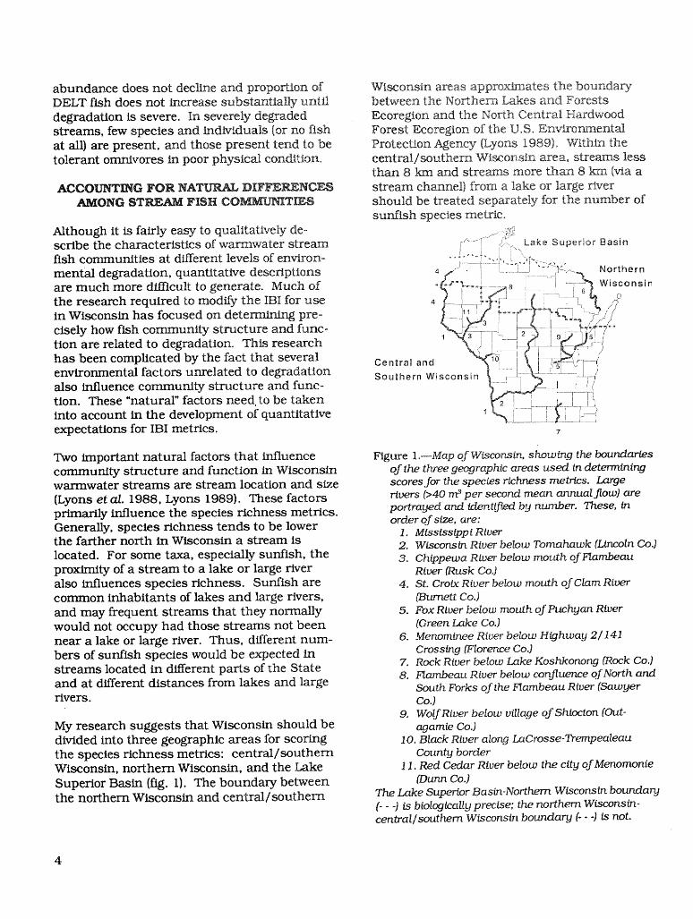
Two important natural factors that influence Figure 1.--Map of Wisconsin, show[ng the boundariescommunity structure and function in Wisconsin of the three geographic areas used in determiningwarmwater streams are stream location and size scores for the species richness metrics. Large

(Lyons et al. 1988, Lyons 1989). These factors rivers (>40 m _per second mean annual flow) areprimarily influence the species richness metrics, portrayed and identified by number. These, in

order of size, are:Generally, species richness tends to be lower I. Mississippi Riverthe farther north in Wisconsin a stream is 2. Wisconsin River below Tomahawk (Lincoln Co.)located. For some taxa, especially sunfish, the 3. Chippewa River below mouth of Flambeauproximity of a stream to a lake or large river River (Rusk Co.)also influences species richness. Sunfish are 4. st. Crolx River below mouth of Clam Rivercommon inhabitants of lakes and large rivers, (Bumett Co.)

and may frequent streams that they normally 5. Fox River below mouth of Puchyan Riverwould not occupy had those streams not been (Green Lake Co.)near a lake or large river. Thus, different num- 6. Menominee River below Highway 2/141bers of sunfish species would be expected in Crossing (Florence Co.)7. Rock River below Lake Koshkonong (Rock Co.}streams located in different parts of the State 8. Flambeau River below confluence of North andand at different distances from lakes and large South Forks of the Flambeau River (Sawyerrivers. Co.)

9. Wolf River below village of Shiocton (Out-My research suggests that Wisconsin should be agamie Co.)divided into three geographic areas for scoring 10. Black River along LaCrosse-Trempealeauthe species richness metrics: central/southern County borderWisconsin, northern Wisconsin, and the Lake 1I. Red Cedar River below the city of Menomonie

Superior Basin (fig. i). The boundary between (Dunn Co.}the northern Wisconsin and central/southern The Lake Superior Basin-Northern Wisconsin boundary

(- - -) is biologically precise; the northern Wisconsin-central/southern Wisconsin boundary (- - -) is not.

The boundary between the Lake Superior Basin PART 2: APPLYING THE IBZ IN WISCONSINand northe_ Wi_:onsin areas is biologically WANa_WATEN STEAMS

precise, delineating the northern range bound-ary" for several fish species in Wisconsin, Application of the V_risconsin tBI is a sequentialStrea_s _n.the Ls,ke Superior Basin tend to process, involving a seSes of discrete steps.have fish connsaunities with ,fewer species than These steps are surmma_ed in table 1 andChose of northern V/iscons.hn streams, discussed in detail below,

Howe'ver, the bounda_-y between the northern COLLECTING AND PROCIgSSlNG TH__Ari_onsin and central/southern Wisconsin F]KgLD DATA

areas is biologically imprecise. Generally,no_,hern Wisconsin fish communities are more telectir_g a_ad Delt_eattrtg Sites f¢_r

depauperate _ species than central/southern Data ColtectionWi_onsin fish communities, but the transition

between these two areas is not as sharp as An appropriate choice of sampling sites is

indicated on figure 1. tn fact, the boundary is critical for the successful application of the IBI.fairly dfdTuse; streams north of the border may The Wisconsin IBI presented here should behave attributes of central/southern Wisconsin used only on %Vlsconsin warmwater streams offish cornrnu:aities, and streams south of the intermediate s_e. More specifically, the Wis-

border rnacy have attributes of northern Wiscon- consin IBI should be applied only to reaches ofsin fish commur_.tfeso permanent streams that are not designated as

trout water and t_hat are between 2.5 and 50 m

In Wisconsin, species richness tends to increase wide with few areas deeper than 1.25 m. It

with increasing stream sLze. The rate at-which must be possible to effectively sample thesespecies richness increases differs depending on stream reaches by wading. The general conceptthe taxa considered. To account< for this in- of the IBI is valid for stream reaches that do not

crease, Maximum Species Richness (MSR) plots meet these criteria, but the Wisconsin IBIhave been developed (see Appendix S) for each presented here has not been tested on them andspecies richness metric, MSR plots predict the may not be appropriate. Note that some sitesmaximum number of species that undegraded with relatively cool water but degraded environ-streams of different s_es should have {Karr et mental conditions have the potential to become

aL 1986). The actual number of species in a trout water ff environmental conditions arestream is compared with the prediction from the improved. The Wisconsin IBI should probably

MSR plot as part o£ the IB! calculation (see Part not be applied to these sites (see Appendix 2].2). Dirt%rent MSR plots are used for the Lake

Superior Basin, northern Wisconsin, and cen- Sites chosen for sampling should be representa-tral/southem Wisconsin_ tive of the overall habitat of the stream reach.

Sampling areas should not normally include

Metrics related to species composition, trophic bridges, dams, mouths of tributaries, or otherand reproductive function, and fish abundance atypical habitat features, u_ess the goal of theand condition are not strong!y influenced by sampling is to characterize the influence ofstream location and s_e; for these metrics, the these atypical features on local environmental

same expectations are used for atl areas of the quality. Fish assemblages in the vicinity ofState and all sbzes of streams (see Part 2). atypical habitat features are often not represen-

tative of the overaI1 fish community of a streamreach.

Table 1.mAn outline of the steps involved in applying the Wisconsin IBI

I. COLLECTING AND PROCESSING THE FIELD DATA

A. Selecting and Delineating Sites for Data CollectionChoose sites on warmwater streams that are 2.5 to 50 m wide and shallowenough to be effectively sampledby wading. Choose sites representative of the stream reach that is to be characterized. Delineate sites with alength of approximately 35 times the average width of the stream.

B. Determining When to SampleSample sitesbetween mid-June and mid-September in central and southern Wisconsin, and during July orAugust in northern Wisconsin. Sample during daylight hours when streams are at baseflow.

C. Determining Stream SizeUse mean stream width within each site as the measure of stream size. Calculate mean stream widths fromat least 10 field measurements per site. Make measurements at baseflow.

D. Sampling the Fish CommunitySample each site thoroughly in an upstreamdirection with a towed eiectroshocker. Carefully sample all majorhabitats within each site, and attempt to capture all fish observed that are greater than 25 mm total length.

E. Processing the Fish SampleAccurately identify all fish to species and count the number of each species captured for each site. Also countthe number of fish with obvious external deformities, eroded fins, lesions, and tumors (DELT).

!1. ANALYZING THE DATA

A. Determining Stream LocationLocateeach sitewiththe three IBi regionsof Wisconsin(Lake SuperiorBasin, northernWisconsin,andcentral/southernWisconsin),and measurethe distance (via streamchannels)from each site to the nearestlake (greaterthan 4 ha) or largeriver(see fig. 1).

B. Classifying Fish SpeciesFor eachsite,classify each fish speciesthatwas caughtintothe appropriateIBI metricgroupingsusingtables2, 3, and 13.

C. Dealing With Very Low Catch RatesDetermineif sufficientfish havebeen capturedto calculatethe IBI. If fewer than 50 fish (includingtolerantspecies)havebeen capturedfrom a site,do not calculatean overallIBI score;ratethe bioticintegrity/environ-mentalqualityof that site asvery poor.

D. Using MSR Plots for ScoringDeterminethe numberof speciescapturedat each sitefor eachof the five speciesrichnessmetrics(nativespecies,darters,suckers,sunfish,andintolerants).Use the appropriateMSR plotsandguidelinesfor scoringeach metric. For sites inthe Lake SuperiorBasin,usetable 4. Forsitesin northernWisconsin,usefigures 2-6. Forsitesin central/southernWisconsin,use figures7-12.

(table I continued on next page)

m

{table 1 continued)

E. Scoring Metrics Based on PercentagesCalculate the remaining five metrics (tolerant species, omnivores, insectivores, top carnivores, simpletithophiis) as percentages (to the nearest 1 percent) of the total number of fish caught at each site. Use theguidelines in table 5 to score these metrics.

F. Scoring Correction FactorsFor each site, calculate the number of individuals per 300 m correction factor as the total number of fishcaught, excluding tolerant species, per 300 m of stream sampled, and the percent DELT fish correction factoras the total number of DELT fish captured divided by the total number of all fish (including tolerant species)captured. Score these two correction factors using guidelines in table 5.

G. Calculating the Overall IBI ScoreDetermine the overall IBI score at each site by summing the scores for the 10 metrics and the 2 correctionfactors. If the overall score is less than zero, round the score up to zero.

Ill. INTERPRETING JBJSCORES

A. Interpreting the Overall IBi ScoreUse the guidelines in table 6 to interpret the overall IBi score for each site. If the overall score is close to 100,then infer that the biotic integrity/environmental quality of the site is high. If the score is near O,then infer thatbiotic integrity/environmental quality is low. If the score is intermediate, then infer that biotic integrity/environ-mental quality is intermediate.

B. Identifying Specific Environmental ProblemsUse scores for individual metrics to suggest specific environmental problems at sites where biotic integrity/environmental quality is intermediate or low.

C. Accounting for Differences Among Samples in IBI ScoresIn comparisons of overall IBi scores from different sites or from the same site over time, assume that differ-ences in scores of 10 points or less are not significant and probably represent the combined effects of sam-pling error and natural variation in biotic integrity. Assume that differences of 25 points or more representclear differences in biotic integrity/environmental quality. Collect further data to indicate whether differences of10 to 25 points are significant.

D. Incorporating Other Types of InformationDo not rely solely on IBi scores when assessing the biotic integrity/environmental quality of sites. Wheneverpossible, also incorporate data on the other biota and the physical and chemical attributes of each site.

The total length of the site is very important, Deterr_tnlng Whets _:_'_Sa_;apleand it will vary dependtr_ on the size andnature of the stream. I:f the site is too short, Sampling should take place between mid-Junecertain uncommon or diDlcult-to-catch species and mid-September in central/sou:them Wis-are likely to be missed. K the site is too long, consin, and during July or August in northern

the amount of effort necessary to complete the Wisconsin and the Lake Superior Basin {:fig.. t).sampling becomes prohibitive. Ideally. the site Sampling during sun.her macdmizes samplingshould be long enough to encompass several ease and minimizes disturbance of springexamples of all the major macrohabitat types spawning gamefish. Additionally, surmnerwithin the reach (/.e., pools, runs, riffles, bends, sampling avoids t2_e potential inclusion ofbackwaters, side channels, islands, log jams). A transient species that may occur during springminimum distance of 35 t_e:s the mean chan- or fall sampling. Many species of fish, including

nel width at normal flow should be sampled to mirmows (family Cyprtnidae), suckers (familyobtain an accurate picture of the fish co_u- Catostomidae) 0smallmouth bass (M_ropterus

nity [Lyons 1992). In other words, ff the stream dolomieu), sauger (Stfzostedfor_ car_ade.ns_o andreach averages 5 m wide at normal flow, then at walleye (Sttzosted_on ugtreum), undertake large-least 175 m of stream should be sampled. K the scale movement or migration during spring and

reach has well-developed, regularly spaced fall (Hall 1972, Curry and Spacie 1979, Schlos-pools, riffles, and runs, then an alternative ser and Ebel 1989, Langhurst and Schoenikesampling distance is three complete adjacent 1990), but appear to stay within a limited homepool-riffle-run sequences. _VVhichever criterion range during the summer (_rirnore t952,is used, the sampling distance should be accu- Gerking 1953, Funk 1955). Angermeier andrately measured and recorded. Karr (198G), Angermeier and Schlosser (t987),

and Karr et aL (1987) analyzed several years ofFor small (fie., narrow) streams, the above data from Illinols streams and concluded that

sampling distance guidelines can be easily met early summer to midsummer was the best time

I in less than 3 hours of sampling, and should to sample for calculation of the IBI.

always be followed. However, the amount oftime required to meet these guidelines for some Sampling should always occur during thelarger streams may be prohibitive {re., more daytime. Although night sampling may be morethan 5 hours), especially ff fish density is high. effective for :some nocturnal species such asIn such cases, site length can be shortened, but bullheads and catfish (family Ictalu_idae) andunder no circumstances should site length for for top carnivores such as smattmouth bass

larger streams be less than 150 m nor should (Paragamian 1989), expectations for all thesampling time be less than 1 hour. metrics in the Wisconsin tBI have been devel-

oped from daytime data, so use of nighttimeAt sites that are wider than 16 m, it is usually data may bias results. Additionally, electro-

Impossible to simultaneously sample the entire shocking by wading is far easier and saferwidth of the channel. At such sites, sampling during the day than at night.

should proceed in a zigzag pattern, moving fromone bank to the other. All areas of hiding cover Sampling should take place when the stream isshould be sampled thoroughly, as well as at baseflow (stable flow in the absence of runoffrepresentative examples of all the major mac- from precipitation). Eleetroshocking at higherrohabitats present, but the entire surface area flows is more difficult and less effective becauseof the site need not be sampled, of greater water volume, stronger currents, and

decreased water clarity_ Sampling should alsobe avoided for at least 2 weeks after a majorflood, even ff water levels quickly return tonormal. Many fish probably vacate their usualhabitat during floods, and it may take themseveral days to return to this habitat after the

flood has ended.

7

8!

))

i!;il ....................................................................llllliillrf"rcfTrr................iiiiillliilrNTrrl,- -T........ I

DCtC_T_i_ing Strcara Size Width measurements should be made at base-flow. K flow is reduced below normal baseflow

In the Wisconsin version of the IBI, mean because of drought, then width measurementsstream width at normal flow is used as the should be based on an estimate of width at

measure of stream size for calculation of species normal flow rather than the actual currentrichness metrics. This differs from other vet- channel width. Usually, the edges of the normalsions of the IBI in which stream order (Karr baseflow channel can be easily determined from

t 981, Karr et ato 1988) or drainage basfin area an examination of channel shape and the{Ohio EPA 1988) is used. I have chosen to use distribution of terrestrial vegetation along themean width in the Wisconsin version for four banks.reasons: {1) stream width is a measure ofstream size more famflia_r to WDNR managers Sampling the Fish Community

and biologists than either Stream order or basLnarea; {2) stream width is a more accurate and Fish sampling should be done with a single

precise measure of stream s_e than stream WDNR-type "stream" electroshocker (generatororder in Wisconsin; (3) stream width was avail- towed in a small boat, with two or three opera-

able in the Fish Distribution Survey data base, tots who wade with hand-held electrodes). Inwhereas stream order and basin area were not; streams less than 4 m wide that are very shal-

{4) stream width is a more consistent measure low or have numerous obstacles to boat move-of stream size between glaciated and unglacl- ment (e.g., large rocks or woody debris, thick

ated regions of Wisconsin than either stream overhanging vegetation), a backpack electro-order or basin area. In examining streams from shocker can be used. Usually, a DC or pulsed-

regions with dtt%erent glacial histories, the best DC output electroshocker is preferred because itmeasure of stream size is probably mean an- is safer, more effective in turbid or deep water,nual discharge {Hughes and Omernik 1981, and lessharmful to fish, but In low conductivity1983). However, discharge data are available water (less than 75 umhos/cm) it may befor only a small fraction of Wisconsin streams, necessary to use an AC unit. Shocking shouldWhen I compared streams of similar discharge be done in an upstream direction for safety

between the unglaciated Driftless Area of Wis- reasons. All habitats within the site should beconsin and the glaciated portions of the State, carefully and thoroughly shocked, and attemptsmean width differed less than either stream should be made to capture all fish observedorder or basin area. Revak [1989) found that greater than 25 mm in total length. Fish

Driftless Area streams had higher stream orders smaller than this are not effectively sampled bybut smaller basin areas than similarly sized electrofishing and should not be used in calcu-streams from glaciated areas of Wisconsin. lation of the IBI. It is particularly Important to

expend the same effort to capture nongameFor use in the IB!, mean stream width should species as to capture gameflsh species. Thebe calculated from at least 10 widely spaced goal is to obtain a representative sample of thefield measurements at the site. These measure- total fish community.

ments should be made with a tape measure,and must have a minimum precision of _+0.3 m. Prc_essing the Fish SampleMeasurements must encompass the range ofwidths present at a site, as well as the major Proper identification of all fish species is essen-main channel macrohabitats that are present tial to accurately determine the IBI. Identifica-

(i.e,, pools, riffles, runs). Side channels should tion of many nongame fish species and juvenilebe part of width meaurements, but islands and game species is difficult in the field, so unlesssand or gravel bars should not, unless they identification is certain, captured fish should behave been exposed by drought and would be preserved for later examination and identfflca-underwater at normal flow (see below). Backwa- tion with keys. For specimens too large to

ters, sloughs, and adjacent wetlands should preserve, good quality photographs are analso not be included in width measurements.

option, but it is important that these photo- assigned to the approp_ate geegraphic area:graphs clearly show the features necessary for Lake Superior Basks, northern Wisconsin, or

accurate identification. The best keys :for central/southern Wisconsin {fig. 1),, Differentidentification of Wisconsin fishes are in Becker criteria are used :for each area in scoring species(1983); other useful keys are Eddy and Under- richness metrics.hill (1974), Pflieger (1975), Smith (1979), andTrautman (1981). Even with good keys, identffi- The boundary between the northern Wisconsincation of many species, especially minnows, is and central/southern Wisconsin areas, whichnot easy and requires patience and practice, corresponds to county boundaries, represents a

relatively broad transition zone rather than aDuring Identification, the total number of fish sharp border. In analyzing species richness

with obvious external deformities, eroded fins, metrics for sites within 40 km of"this boundarylesions, and tumors should be counted for (via stream channels), I recommend calculatingcalculating the percent DELT fish correction two IBI scores, one using the expectations forfactor. It is important to distinguish between northern Wisconsin and the other -using expec-damage to fish caused by poor environmental rations for central/southern Wisconsin. The

quality and damage to fish caused by electro- score and rating that seem most reasonableshocking or preservation, which should not be based on overall fish community attributes [seeincluded in the count. Electroshocking, espe- Interpreting IBI Scores on page 23) should becially with AC current, sometimes causes large used.gashes or burns on fish, and may break bones,leading to apparent deformities (personal obser- In the central/southern Wisconsin area, thevations). Poor or incomplete preservation can scoring criteria for the sunfish species richness

lead to sloughing of scales and breakage of fins. metric depend on the distance of the samplingSome parasites that occur just under the skin site {via stream channels) from a lake greatersurface on fish may expand upon preservation, than 4 ha or a river with a mean annual dis-

and the bump on the skin that results may charge of 40 m a per second (see fig. 1). Thissuperficially resemble a tumor. All of these distance should be determined from 7.5 minute

electroshocking and preservation artifacts can (1:24000 scale) topographic maps using a mapbe distinguished from true deformities, eroded wheel. If the distance is less than or equal to 8fins, lesions, and tumors with careful observa- km, then one MSR plot is used to score thetlon and dissection. Note also that during and metric; if the distance is greater than 8 kin,immediately after the spawning season, breed- then another MSR plot is used.ing individuals of many species may appear"beat up" as a result of spawning activities; Classlfytr_g Fish Speciessuch individuals should not be Included In the

count of DELT fish. To score the IBI metrics, all fish in a sample

from a site must be classified into the appropri-ate structural and functional groups. Each

AlgALYZING THE DATA metric consists of the fish that belong to a singlestructural or functional group. Individual fish

Determining Stream Locatton species may be part of more than one group andhence contribute to more than one metric. A

Information about stream location is necessary complete classification of all fish species infor the calculation of species richness metrics. Wisconsin can be found in Appendix 4. TheThe location of each sampling site should be metrics and groups are as follows:precisely described, including drainage basin,county, legal description (township, range, Species Richness and Composgtfon Metricssection), and distance from permanent land-

marks, such as bridges, roads, or towns. It is Total number of native species--The totaloften useful to prepare a map of the sampling number of species collected at a site, excludingsite and surrounding area. Each site should be hybrids (which can be common among sunfish

10

and ce_ain species of minnows) and exotic flavescens) are included tn this metric. Yellowspecies (table 2). Exotic species are species that perch are widespread in this area, and occupyare present in Wisconsin waters only because of an ecological niche generally similar to that ofdirect introduction by humans (eog., carp, sunfish.salmon) or because of recent invasions that

would not have been possible without human Number of tnto|era_t apecies---The totalintervention (eog., the sea lamprey and alewife number of species, excluding hybrids, that areir_vaded Lake Michigan and Lake Superior after intolerant of environmental degradation, par-the construction of the Weiland Canal, which ticularly poor water quality, siltation and in-bypassed Niagara Falls, a barrier to fish move- creased turbidity, and reduced habitat heteroge-ment), neity (e.g., channelization). Intolerant species

exist in a wide variety of fish families (table 2).Number of darter species--The total number of However, delineation of intolerant species is adarter species (family Percidae, table 2) col- somewhat subjective process, and the criterialected, excluding hybrids. Darters are small used in delineation are not easily quantified. Ibenthic species that tend to be intolerant of used three qualitative criteria, listed in order ofmany types of en_dronmental degradation. They priority, to classify species as intolerant: (1} aare mainly insectivorous, and for many of them, known high degree of sensitivity to the types ofriffles or runs are preferred habitat. In the Lake environmental degradation listed above, asSuperior Basin, where darter species richness is documented in Becker (1983) and other regionalnaturally low, sculpins (Cottus species) and fish publications; (2) an observed major declinemadtoms (Notucus species) are included in this in distribution and abundance in regions ofmetric. Sculpins and madtoms are commonly Wisconsin where environmental problems areencountered in warmwater streams of this area, known to be severe (urban and industrial areas,

and occupy an ecological niche generally similar agricultural areas with serious nonpoint sourceto that of the darters (see also Steedman 1988). pollution problems); (3) designation as intoler-

ant in other versions of the IBI used in central

Nt_raber of sucker species---The total number North America.of sucker species (family Catostomidae, table 2)collected, excluding hybrids. Suckers are large Percent that are tolerant species--The num-benthic species that generally live in pools or ber of Individuals that are members of speciesruns, although a few species are common in classified as tolerant of environmental degrada-riffles. Some species are intolerant of environ- tton (table 2), expressed as a percentage of themental degradation, whereas others are toler- total number of fish captured. As is the case forant. Most species feed on insects, although a intolerant species, the delineation of tolerantfew will also eat large quantities of detritus or species is somewhat subjective. I used threeplankton, qualitative criteria, listed in order of priority, to

classify species as tolerant: (1) a known abilityNumber of sunfish species--The total number to withstand poor water quality, particularly lowof sunfish species (family Centrarchidae, table dissolved oxygen levels, high levels of ammonia2), including rock bass (Ambtoptites rupestrts} and other toxic substances, and high turbidity,and crappies (Pomoxis species}, but excluding as documented in Becker (1983) and otherhybrids and smallmouth and largemouth bass regional fish publications; (2) an observed(Micropterus salmoides). Sunfish are medium- ability to persist in good numbers in Wisconsinsized, midwater species, which tend to occur in streams with poor environmental quality; (3}pools or other areas of slow-moving water, designation as tolerant in other versions of theMost, but not all, are moderately tolerant of IBI used in central North America. Hybrids areenvironmental degradation. All feed on a variety included in this metric ff one or both parentalof invertebrates, although after some sunfish species are considered tolerant species.

reach a certain size, they will eat fish. In theLake Superior Basin, where sunfish species

richness is naturally low, yellow perch (Perca

11

i, i I I I --

Table 2.--Species asslgruments for species richness and composition metrics _

Group Species

Exotic species Sea Lamprey, Alewife, PinkSalmon, Coho Salmon, Chinook Salmon, Atlantic Salmon,Rainbow Trout, Brown Trout, Rainbow Smelt, Goldfish, Common Carp, Grass Carp, Rudd,Threespine Stickleback, White Perch, Ruffe

Darters Crystal Darter, Western Sand Darter, Mud Darter, Rainbow Darter, Bluntnose Darter, IowaDarter, Least Darter, JohnnyDarter, Banded Darter, Logperch, Gilt Darter, Blackside Darter,Slenderhead Darter, River Darter

Suckers Highfin Carpsucker, Quillback, River Carpsucker, Longnose Sucker, White Sucker, BlueSucker, Creek Chubsucker, Lake Chubsucker, Northern Hog Sucker, Spotted Sucker,Smallmouth Buffalo, Bigmouth Buffalo, Black Buffalo, Silver Redhorse, River Redhorse, BtackRedhorse, Golden Redhorse,Shorthead Redhorse, Greater Redhorse

Sunfish Rock Bass, Green Sunfish, Pumpkinseed, Bluegill, Warmouth, Orangespotted Sunfish,Longear Sunfish, White Crappie, Black Crappie

Intolerant species Chestnut Lamprey (ammocoeteonly), Northern Brook Lamprey, Southern Brook Lamprey,Silver Lamprey (ammocoete only), American Brook Lamprey, Sea Lamprey (ammocoeteonly), Brook Trout, Muskellunge, RedsideDace, Mississippi Silvery Minnow, Speckled Chub,Gravel Chub, Pallid Shiner, Pugnose Shiner, Ghost Shiner, Blackchin Shiner, BlacknoseShiner, Spottail Shiner, Rosyface Shiner, Weed Shiner, Ozark Minnow, Highfin Carpsucker,Blue Sucker, Northern Hog Sucker, Black Buffalo, Spotted Sucker, Greater Redhorse, Slen-der Madtom, Rock Bass, Longear Sunfish, Smallmouth Bass, Crystal Darter, Rainbow Darter,Iowa Darter, Least Darter, Gilt Darter, Slenderhead Darter, Mottled Sculpin, Slimy Sculpin,Spoonhead Sculpin, DeepwaterSculpin

Tolerant species Central Mudminnow, Goldfish, Common Carp, Golden Shiner, Red Shiner, Bluntnose Min-now, Fathead Minnow, Blacknose Dace, Rudd, Creek Chub, White Sucker, Yellow Bullhead,Green Sunfish

Scientific names for this and table 3 are given in Appendix 4 table 13.

12

Table 3._Spectes assignments for trophtc and reproductive function metrics

Group Species

OmnivoFes Goldfish, Common Carp, Golden Shiner, Red Shiner, Biuntnose Minnow, Fathead Minnow,Bullhead Minnow, Rudd, River Carpsucker, Quillback, Highfin Carpsucker, White Sucker

Insectivores Lake Sturgeon, Shovelnose Sturgeon, Goldeye, Mooneye, LakeWhitefish, Round Whitefish,Pygmy Whitefish, Central Mudminnow, Redside Dace, Lake Chub, Speckled Chub, Silver Chub,Gravel Chub, Homyhead Chub, Pallid Shiner, Emerald Shiner, River Shiner, Ghost Shiner,]roncolor Shiner, Striped Shiner, Common Shiner, Bigmouth Shiner, Pugnose Minnow, Black-chin Shiner, Blacknose Shiner, Spottaii Shiner, Rosyface Shiner, Spotfin Shiner, Sand Shiner,Redfin Shiner, Mimic Shiner, Suckermouth Minnow, Finescale Dace, Longnose Dace, PearlDace, Longnose Sucker, Blue Sucker, Creek Chubsucker, Lake Chubsucker, Northern HogSucker, Smatlmouth Buffalo, Bigmouth Buffalo, Black Buffalo, Spotted Sucker, Silver Redhorse,River Redhorse, Black Redhorse, Golden Redhorse, Shorthead Redhorse, Greater Redhorse,Black Bullhead, Yellow Bullhead, Brown Bullhead, Stonecat, Slender Madtom, TadpoleMadtom, Pirate Perch, Troutperch, Banded Killifish, Blackstripe Topminnow, Starhead Topmin-now, Brook Silverside, Brook Stickleback, Ninespine Stickleback, Threespine Stickleback, WhitePerch, Green Sunfish, Pumpkinseed, Bluegill, Orangespotted Sunfish, Longear Sunfish, CrystalDarter, Western Sand Darter, Mud Darter, Rainbow Darter, Biuntnose Darter, Iowa Darter,Fantail Darter, Least Darter, Johnny Darter, Banded Darter, Ruffe,Yellow Perch, Logperch, GiltDarter, Blackside Darter, Slenderhead Darter, River Darter, Freshwater Drum, Mottled Sculpin,Slimy Sculpin, Spoonhead Sculpin, Deepwater.Sculpin

Top carnivores Longnose Gar, Shortnose Gar, Bowfin, American Eel, Skipjack Herring, Pink Salmon, CohoSalmon, Chinook Salmon, Atlantic Salmon, Rainbow Trout, Brown Trout, Brook Trout, LakeTrout, Northern Pike, Grass Pickerel, Muskellunge, Channel Catfish, Flathead Catfish, Burbot,White Bass, Yellow Bass, RockBass, Warmouth, Smailmouth Bass, Largemouth Bass, WhiteCrappie, Black Crappie, Walleye, Sauger

Simple Lake Sturgeon, Shovelnose Sturgeon, Paddlefish, Redside Dace, Lake Chub, Gravel Chub,Iithophilous Emerald Shiner, River Shiner, Striped Shiner, Common Shiner, Ozark Minnow, Rosyfacespawners Shiner, Suckermouth Minnow, Southern Redbelly Dace, Biacknose Dace, Longnose Dace,

Longnose Sucker, White Sucker, Blue Sucker, Northern Hog Sucker, Silver Redhorse, RiverRedhorse, Black Redhorse, Golden Redhorse, Shorthead Redhorse, Greater Redhorse, Burbot,Crystal Darter, Rainbow Darter, Banded Darter, Logperch, Gilt Darter, Blackside Darter, Slen-derhead Darter, River Darter, Walleye, Sauger

13

Trophic and Reproductive t?_nction Metrics Percent that are top ear_xtvores ..........the nurnberof individuals that belong to species with an

Percent that are omnivores--The number of adult diet dominated by vertebrates (especiallyindividuals that belong to species with an adult fish) or decapod crustacea {eogo, crayfish,diet consisting of at least 25 percent {by volume) shrimp) (table 3), expressed as a percentage ofplant material or detritus and at least 25 per- the total number of fish captured° Species thatcent live animal matter (table 3), expressed as a have a predominantly piscivorous diet onlypercentage of the total number of fish captured, when they reach very large size (eog., creekBy definition, omnivores can subsist on a broad chub) are not considered top carnivores for thisrange of food items, and they are relatively metric. Hybrids are considered top carnivoresinsensitive to changes In the food base of a only ff both parental species are top carnivores.stream caused by environmental degradation.Primarily herbivorous species that occasionally Percent that are simple lttl_opl_ilot_s sl)awn-ingest significant proportions of animal matter ers_The number of individuals that belong to

(e.g., stonerollers [Carnpostoma species]) are not species that lay their eggs on clean gravel orconsidered omnivores for this metric. Trophic cobble and do not build a nest or provide paren-classifications for this and the two other trophic tal care (table 3), expressed as a percentage offunction metrics are based upon personal the total number of fish captured. Simpleobservations, data in Becket (1983), and trophic lithophflous species need clean substrates forclassifications in Karr et al. (1986) and Ohio spawning and are particularly sensitive toEPA (1988). Hybrids are included as omnlvores sedimentation of rocky subs(rates. Classffica-If one or both parental species are omnivores, tlon of species as simple lithophilous spawners

is based on Balon (1975), Berkman and Rabenil%rcent that are tnsectlvores_The number of (1987), and Ohio EPA (1988). Hybrids areindividuals that belong to species with an adult considered simple lithophflous spawners only ffdiet that is normally dominated by aquatic or both parental species are simple lithophilousterrestrial insects (table 3), expressed as a per- species.centage of the total number of fish captured.Species classified as omnlvores are not consld- Fish Abundance and Condition Correctionered insecttvores even if they eat large numbers Factorsof insects, nor are obligate filter feeders thatmay eat drifting insects (e.g., g _izzard shad Nc_r_ber of individuala-_Fhe number of indlvld-[Dorosoma cepedianum]). However, species that ual fish, exelutling individuals of tolerant spe-may be primarily insectivorous under some cies, captured per 300 m of stream sampled.

circumstances, and planktivorous (e.g., bluegill To calculate this value, multiply the number of[Lepomis macrochirus]) or molluscivorous (e.g., individuals captured {minus the tolerant indl-pumpklnseed [Lepomis gibbosus], freshwater viduals) times 300 and then divide by thedrum [Aplodinotus grunntens]) under others, are distance sampled in meters. The number ofconsidered lnsectlvores for this metric. The individuals per 300 m Is consistently very low at

creek chub (Semotilus atromaculatus) and highly degraded sites, but may be either high orlow at moderately or lightly degraded sites (seeblacknose dace (Rhinichthys atratulus) are

considered generalized invertivores rather than Appendix 1).insectivores, and they are not Included in thismetric. Although their diet is often dominated Percent with deformities, eroded fins, le-by Insects and they rarely consume plant atons, or tu_ors (DELT)--The number ofmaterial, these two species eat a very broad individual fish with skeletal or scale deformities,range of animal matter, and they respond to heavily frayed or eroded fins, open skin lesions,changes in the food base of a stream more as an or tumors, that are apparent from an externalomnivore than an Insectivore (Ohio EPA 1988). examination, expressed as a percentage of the

Hybrids are counted as insectlvores only ff both total number of fish captured. Fish with heavyparental species are insectivores, parasite burdens (e.g., infestations of black spot

14

[Neascus sp.] or anchor hookwoITn [Lemea sp.]) The first step in using MSR plots is to convertare not included as DE_[' fish unless the para- stream s_e to the proper unit of measure. MSRsites have caused defo_nities or lesions. Fish plots are based on the natural logarithmwith DELT anomalies that are o_fly visible a[_er (base e) of the mean stream width of a site in

dissection are also not included. DELT fish are meters. Most calculators have a function keynormally rare except at highly degraded sites that directly determines natural logarithms; al-(see Appendix 1). ternatively, log tables are available in many

math and statistics textbooks.Dealing Wigh Very Low Catch Rages

Once the natural logarithm of stream width forIf the total number of fish captured from a site a site is determined, the number of species at(including toierant species) is very low, IBI that site should be calculated for each of thescores may be biased and not representative of five species richness metrics. Then, for eachthe tFae biotic integrity and environmental metric, the point that represents the lntersec-quality of the site. W_en a sample contains tion of the natural logarithm of stream width (xonly a few fish, IBI metrics and correction axis) and the number of species (y axis) shouldfactors (especlally those that are based on be located on the appropriate MSR plot. Figurespercentages) may be unduly irffluer_ced by the 2 to 6 give the five MSR plots for sites in north-presence or absence of a few individuals. As a ern Wisconsin, and figures 7 to 12 give the sixrule of thumb, the IBI should not be calculated MSR plots for sites in central and southern Wis-for sites where the total sample consists of less consin (there are two plots for the number ofthan 50 individuals. At sites where fish abun- sunfish species, one for sites within 8 km of adance is yew low, it may be worthwhile to lake or large river, and one for sites more than 8extend the sampling distance to the point where km from a lake or large river). Plots are notat least 50 landividuats have been captured. If given for sites in the Lake Superior Basin.this is not possible or desirable, then the IBI Rather, because of the simplicity of the relation-should not be calculated, and instead, the low ship between stream size and expected numberfish abundance ltseg should be used to assess of species, table 4 gives scoring criteria for threebiotic integrity (see section on Interpreting IBI size classes of streams.Scores).

Once the species richness for a particularUsing MSR Plots For Seori_ag metric has been located on the appropriate MSR

plot, that metric can be scored. Note that eachThe five species richness metrics are scored MSR plot has three diagonal or diagonal/using Maximum Species Richness (MSR) plots horizontal lines. The uppermost of these linesgiven in figures 2 to 12. These MSR plots relate is the Maximum Species Richness Line, the lineexpected numbers of species to stream size at below it is the First Trisection Line, and the llnedifferent levels of environmental quality. Differ- below that is the Second Trisection Line. Theent MSR expectations have been developed for position of the Maximum Species Richness Lineeach of the three geographic areas of Wisconsin, determines the positions of the two Trisectionand within these areas, for each of the five Lines (see Appendix 3 for information on howmetrics. As a rule, at any given stream size, the these lines are generated). If species richnessbetter the environmental quality, the greater the falls on or above the Maximum Species Rich-number of species expected. Additionally, for a hess Line, or between the Maximum Speciesgiven level of environmental quality, the larger Richness line and the First Trisection Line,the stream size, the greater the number of then species richness is similar to that of aspecies expected. Thus, large, high-quality high-quality, relatively undegraded stream, andstreams should have large numbers of species, the metric is scored a 10. If species richnesswhereas small, pooroquallty streams shouldhave few species.

15

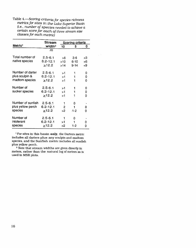
Table 4.--Scoring c_eria for species richnessmetrics for sites in the Lake Superior Basin(i.e., number of species needed to achieve acertain score for each of three stream sizeclasses for each metric)

Stream Scodn criteriaMetric 1 width 2 10 5 0

m

Total number of 2.5-6.1 >6 3-6 <3native species 6.2-12.1 >10 6-10 <6

>-12.2 >14 9-14 <9

Number of darter 2.5-6.1 >1 1 0

plus sculpin & 6.2-12.1 >1 1 0madtom species >_12.2 >1 1 0

Number of 2.5-6.1 >1 1 0sucker species 6.2-12.1 >1 1 0

>_12.2 >1 1 0

Number of sunfish 2.5-6.1 1 0 -plus yellow perch 6.2-12.1 2 1 0species >-12.2 >2 ,1-2 0

Number of 2.5-6.1 1 0 -intolerant 6.2-12.1 >1 1 0

species >12.2 >2 1-2 0

i For sites in this basin only, the Darters metricincludes all darters plus any sculpin and madtomspecies, and the Sunfish metric includes all sunfishplus yellow perch.

2 Note that stream widths are given directly inmeters, rather than the natural log of meters as isused in MSR plots.

16

40 .............................................................................................................. 9 [[ Darter Species - Northern Wisconsin

Total Native Species - Northern Wisconsin 8 I-

]32:" 7i

5 , v,-2s o 10

93 _ 5 _ Y-5.O

._ 10i /" Y=_7__.../ ,,-,., 7z

Z i Y=8.3 2 2 Y-I.Z 2

0 ..............• ............................................J-..............................a ....................... 0 ___L ........... ___ " _O.O0 0.80 1.60 2.40 3.20 4.00 0.00 0.80 1.60 2.40 3.20 4.@0

Natural Log of Mean Width (m) Natural Log of Mean Width (m)

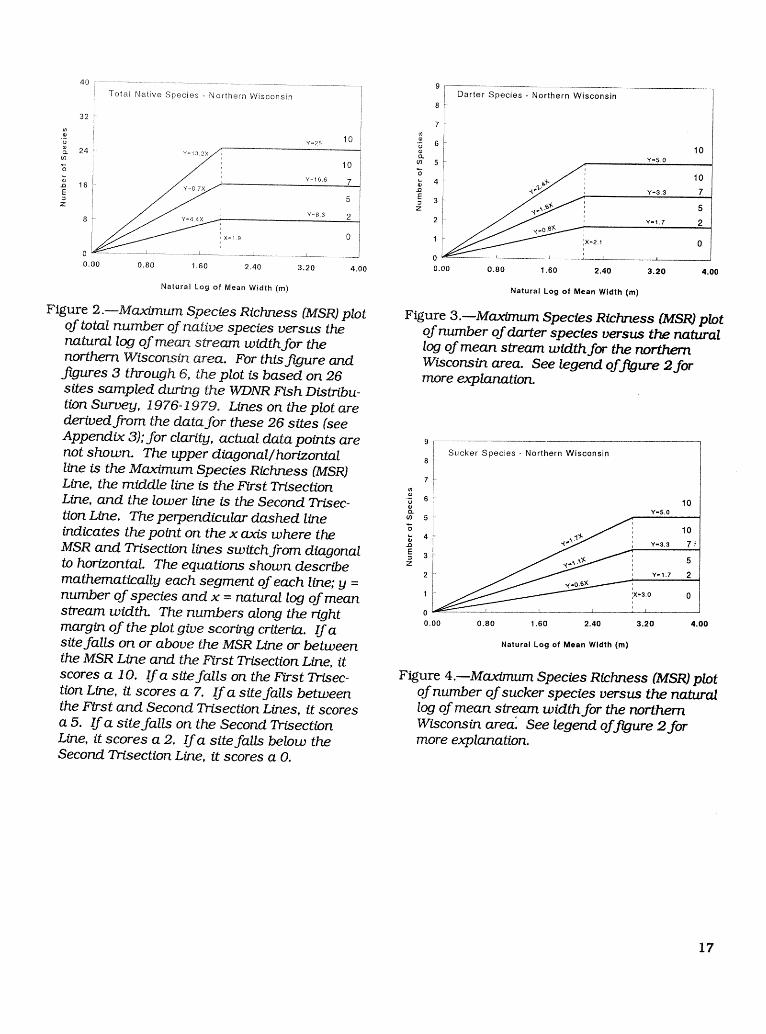
Figure 2.wMaxtmum Species Richness (MSR) plot Figure 3._Maximum Species Richness (MSR) plotof total number of native species versus the of number of darter species versus the naturalnatural log of mean stream width for the log of mean stream width for the northernnorthern Wisconsin area. For this figure and Wisconsin area. See legend of figure 2forfigures 3 through 6, the plot is based on 26 more explanation.sites sampled during the WDNR Fish Distribu-tion Survey, 1976-1979. Lines on the plot arederived from the data for these 26 sites (seeAppendix 3); for clarity, actual data points are 9

! Sucker Species - Northern Wisconsin

not shown. The upper diagonal 8line is the Maximum Species Richness (MSR) t7F

Line, the middle line is the F_rst Trisection _ iLine, and the lower line is the Second Trisec- _ 6 i _o_- i Y-S.otion Line. The perpendicular dashed line _ s F

indicates the point on the x axis where the _ [I i Y-_ _0MSR and Trisection lines switch from diagonal 41

to horizontaL The equations shown describe z 2 i.... Y-,, 2mathematically each segment of each line; y = ! "_-° 'number of species and x = natural log of mean _ i ix-_o ostream width. The numbers along the right o '0.00 0.80 1.60 2.40 3.20 4.00

margin of the plot give scoring criteria. If asite falls on or above the MSR Line or between NaturalLogofMeanWidth(m)

the MSR Line and the First Trisection Line, it

scores a 10. If a site falls on the First Trisec- Figure 4._Maximum Species Richness (MSR) plottion Line, it scores a 7. Ira site falls between of number of sucker species versus the naturalthe FYrst and Second Trisection Lines, it scores log of mean stream width for the northern

a 5. Ifa site falls on the Second Trisection Wisconsin area. See legend of figure 2forLine, it scores a 2. If a site falls below the more explanation.Second Trisection Line, it scores a O.

17

91.............................................................................................................................................................40[........................................................................................................................, Sunfish Species - Northern Wisconsin Total Native Species - Central/Southern Wisconsin

8]- 10Y=30

•_ 6 I- ._ lor_ _ _. 24

¢0e3 5 _ ¥,,,20 7"s i "s

1 ,J _ _8 5•., 3 F :_ v=10 2z

I '°2 F ._ _ _'_ -- 8- " , 1o ,

_, , Y-13 zj

1 -. __ [ .... .b.i

0,00 0.80 1.60 2,40 3.20 4,00 0.00 0.80 1.60 2.40 3.29 4,00

Natural Log of Mean Width (m) Natural Log of Mean Width (m)

Figure 5.wMaximurn Species Richness (MSR) plot Figure 7.wMaximum Species Richness (MSR) plotof number of sunJ'is h species versus the of total number of native species versus thenatural log of mean stream width for the natural log of mean stream width for the cen-northern Wisconsin area. See legend of figure tral/ southern Wisconsin area, For this figure2for more explanation, and flgures 8, 9, and 12, the plot ts based on

435 sites sampled during the WDNR _shDistribution Survey, 1976-I979. Lines on theplot are derived from the data for these 435

9 _............................................................................................................................................................................................sites (see Appendix 3);for clarity, actual data] Intolerant Species - Northern Wisconsin points are not shown. See legend of figure 2

8 1

I for more explanation.7I 10

'G 6 I ¥°_,o

_. i _ _o

'_ 4 !,. Y=4.0 7. 8 Darter Species - Central/Southern Wisconsin

E i s= 3 " 7

z _ ', Y . 102l, / 111"- : _o_,o2 t, ¥_.o_- 10

1 Xo,32 0 {/3 5

0 .................................... '_ Y=4.0 7'- 40.00 0.80 1.60 2.40 3.20 4.00 -_

=E 3 ', 5

Natural Log of Mean Width (m) z ,: Y=2.0 22

Figure 6.--Maximum Species Richness (MSR) plot _ :×°"_ oof number of intolerant species versus the o ......................natural log of mean stream width for the 0.00 0.80 1.60 2.40 3.20 4.00northern Wisconsin area. See legend of figure NaturalLog ofMeanWidth(m)

2for more explanation. Figure 8._Maximum Species Richness (MSR) plotof number of darter species versus the naturallog of mean stream width for the central/southern Wisconsin area. See legends of

figures 2 and 7for more explanation.

18

Sucker Species - Central/Southern Wisconsin f Sunfish Species- Central/Southern Wisconsin

8 ' 8 i Far From Lake or Large River10Y=70 /

7 7[

!_. , Q. /

o0 5 } Y=4.7 7 o_ 5 I' , 10"S I "8 , Y4oj : 5] .a ' 10

:mE 3i ' i E t I Y=2,Z 7z i Y<3 2 j 2- 3 / _"2 ,_,0. [ [ 2 I i

I X=2.5 0 l , Y=1.3 2

1 , i 1 _-0.5! i J ;x=_4s 0

o o '0.00 0.80 1,60 2.40 3.20 4.00 0.00 0.80 1,60 2.40 3.20 4.00

Natural Log of Mean Width (m) Natural Log of Mean Width (m)

Figure 9.--Maximum Species Richness (MSR) plot Figure 11.--Maximum Species Richness (MSR)of number of sucker species uersus the natural plot of number of sunfish species versus thetog of mean stream w_dth for the central/ natural tog of mean stream width for sitessouthern Wisconsin area. See legends of more than 8 km (via stream channels)from afigures 2 and 7for more explanation, lake (> 4 ha surface area) or large r_ver (2_40

mJ per second mean annual discharge) in thecentral�southern Wisconsin area. Lines on

the plot are derived from the data from 2789 _.........................................................................................................................................,

SunfishSpecies- Central/Southern Wisconsin sites;for clarity, these actual data points are8 i NearLakeor LargeRiver not shown. See legend of figure 2for more7_ explanation.

"'5 610

CO 5 b Y=5.0

*,Q Y=3.3 _Z.7 i Intolerant Species 10

E 3 8 _" Central/Southern Wisconsin

1 i/J_,; p'_ x _1 0 '_ 6 / ', Y_5,3 7

0 ' ' ' _ 5 -

0.00 0.80 1.60 2.40 3.20 4.00 "6 /. ,q,._,,,- ii_, 4!- 5" i / %->" '

Figure ZO._Max/mum Species Richness (MSR) 2

__ ×_ 0plot of number of sunfish species versus the _natural tog of mean stream width for sites less o _ .........................................._ _ ,than or equal to 8 km (via stream channels) 0.0o 0.80 1.6o 2.4o 3.20 4.00

from a lake (> 4 ha surface area) or large river Nat,ra_Logof Mean Width(m)(> 40 m 3 per second mean annual discharge)in the central�southern Wisconsin area. Lines Figure 12._Maximum Species Richness (MSR)on the plot are derived from the data from 157 plot of number of intolerant species versus thesites;for clarity, these actual data points are natural tog of mean stream width for the cen-not shown. See legend of fkgure 2for more tral/southern Wisconsin area. See legends ofexplanation, figures 2 and 7for more explanation.

19

falls directly on the First Trisection Line, thenspecies richness is similar to that of a slightly Percentages are calculated by dividing thedegraded stream, and the metric is scored a 7. number of fish within a particular metric groupIf species richness falls between the First and by the total number of fish (including tolerantSecond Trisection Lines, then species richness species) captured from a site° All percentagesls similar to that of a moderately degraded should be rounded to the nearest 1 percent.stream, and the metric Is scored a 5. If species Scoring is based on criteria given in table 5.richness falls directly on the Second TrisectionLine, then species richness is similar to that of a ScoringCorrection Factorsdegraded stream, and the metric is scored a 2.If species richness falls below the Second Tri- The number of individuals captured per 300 msection Line, then species richness is similar to of stream sampled and the percentage of DELTthat of a highly degraded stream, and the metric fish correction factors only influence the overallls scored a 0. IBI score when they have extreme values (table

4). These two correction factors can lower the

As a brief example, consider a site in the cen- overall IBI score, but not improve it. The num-tral/southern Wisconsin area with a mean ber of individuals captured correction factorwidth of 5 m (natural log = 1.61) that Is located includes all fish except tolerant, species.within 8 km of a 80-ha lake. The site has 21 Thus, it is possible to catch a large number oftotal native species, including 2 darter species, tolerant fish from a site and still calculate a veryand 1 sunfish species. The appropriate MSR low or zero value for number of individualsplots for this site are found in figure 7 for the captured (see Appendix 5). If the number oftotal number of native species metric, figure 8 individuals captured per 300 m of stream is lessfor the number of darter species metric, and than 50, the score for this correction factor isfigure 10 for the number of sunfish species - 10; ff it is 50 or greater, the score is 0.metric. The total number of native species fallsJust above the First Trisection Line in figure 7. The percentage of DELT fish ls calculated usingThus, the total number of native species metric all fish captured, including tolerant species. ToIs scored a 10 for this site. The number of determine this percentage, the number of DELT

darter species falls on the Second Trisection fish captured is divided by the total number ofLine in figure 8, so the number of darter species fish captured. If the percentage is greater thanmetric scores a 2. The number of sunfish or equal to 4 percent, the score for this correc-species falls below the Second Trisection Line in tion factor is -10; ff it is less than 4 percent, thefigure 10, so the number of sunfish species score is 0.metric ls scored a 0. A more complete set ofexamples of scoring of all metrics is given in Calculating the Overall IBI ScoreAppendix 5.

The overall IBI score is the sum of the scores for

Scoring Metrics Based on Percentages the I0 metrics and the 2 correction factors. Ifthis sum is less than 0 (i.e., if the sum of the 2

The remaining five metrics, dealing with species correction factors is greater than the sum of thecomposition and trophic and reproductive 10 metrics, yielding a negative overall sum),function, are based on percentages of individual then it is rounded up to 0. Thus, the minimumfish captured rather than number of species, possible overall IBI score is 0, representing veryThese metrics are not strongly influenced by poor biotic integrity, and the maximum is I00,stream size or site location either within Wis- representing excellent biotic integrity.consin or relative to lakes and large rivers.Thus, the same scoring criteria are used for a11sites in Wisconsin.

2O

TabIe 5.---Scoring cr_erta for the t 0 metrics and 2 correct_n factors used to cal-cuJate the W_'_corts_ uers_n of the IBP

Scorln_ criteda_J_etdc or coG'ection factor" 10 7 5 2 0

Species R_chness and Composition Metrics

Total number of native species Scoring for species richness metrics depends onNumber of darter species stream size and location. For sites in theNumber of sucker species Lake Superior Basin, see table 4. For sites inNumber of sunfish species Northern Wisconsin, see figs. 2-6. For sites inNumber of intolerant species Central/Southern Wisconsin, see figs. 7-12.Percent tolerant species 0-19 20 21-49 50 51-100

Trophic and Reproductive Function MetricsPercent omnivores 0-19 20 21-39 40 41-100Percent insectivores 100-61 60 59-31 30 29-0Percent top carnivores 100-15 14 13-8 7 6-0Percent simple Hthophils 100-51 50 49-21 20 19-0

F_sh Abundance and Condition Correction FactorsNumber of individuals per 300 m2 If < 50 fish, subtract 10 from overall IBI scorePercent DKLT fish 3 If > 4 percent, subtract 10 from overall IBi score

1All percents are in terms of total number of fish (inciuding tolerant species); incalculating, round all percentages to the nearest 1 percent.

2The number of individuals correction factor does not include tolerant species.3 Percent DELT fish refers to fish with deformities, eroded fins, lesions, or tumors.

21

L_TERPR]_TLWG _I SCORES Xdentifylng Speclflc E_vh'on_e_$al Problems

Iritell_reting tile Overall l[Bl Score l_e over'all IBI score is a measure of the overallenvironmental quality of a stream site, and a

The higher the overall IBI score, the better the tow score indicates that environmental problemsbiotic integrity and, by inference, the environ- exist_ By itself, the overall tBI score cannotmental quality of a site. Sites with !BI scores reveal what these problems are, However, theclose to the maximum possible value of I00 scores of individual metrics often provide insightpresumably have excellent environmental into the specific causes of enviroxcmentai degra-quality, whereas sites with tBI scores close to dation. For instance, tow numbers of simplethe minimum possible value of 0 presumably lithophilous species and benthic species such

have very poor environmental quality. Sites as darters and suckers are often caused bywith intermediate scores presumably have siltation and loss of coarse substrate. Sunfishintermediate environmental quality, Table 6 and top carnivores do best in deeper pool

provides integrity ratings for different ranges of habitats and areas of extensive cover, so if theiroverall IBI scores, species richness and abundance are low, deep

water and instream cover habitat may have

The overall IBI score is a useful summary of a been lost. High numbers of DELT individuals

wide and complex range of fish community invariably indicate major water quality prob-attributes at a site. However, like all summaries lems. Highly skewed relative abundances of

of complex situations, the overall IBI score feeding groups can reflect disruptions of foodsometimes oversimplifies or misrepresents webs. Karr et at. (1985, 1986), Berkman et al.reality. Therefore, it is important not to rely too (1986), Leonard and Orth {1986), Ohio EPAheavily on the overall IBI score when assessing {1988), and Steedman (1988) provide examplesbiotic integrity. Of more value are the integrity of how metric scores can be used to infer spe-rating derived from the IBI score and the actual cfflc types of environmental degradation.nature of the fish community (Karr et al. 1986).Attributes of fish communities that are repre- Accoanting for Differences A_ong Samples

sentative of very poor to excellent biotic integrity in IBI Scoresare given in table 6, and have been described inthe section "Using and Interpreting the IBI." Even when true biotic integrity and environ-These attributes should be used to check the mental quality of a site remain constant over a

validity of biotic Integrity ratings derived from time period, multiple fish community samplesoverall IBI scores, from that site made over that time period will

rarely all have the same overall IBI score. This

At some sites, the catch of fish {including temporal variation among samples in IBI scorestolerant species) may be too low {fewer than 50 is caused by two factors: sampling error andIndividuals) to permit calculation of the IBI. natural variations in fish community attributes.Assuming that sampling procedures and per- Sampling error represents the failure to accu-formance have been adequate, an extremely low rarely and precisely characterize the fish corn-catch rate In a permanent, lntermedlate-slzed, munity because of sampling difficulties orWisconsin warmwater stream is always an limitations. Natural variations are real fluctua-indication of a serious environmental problem, tions in fish community attributes that resultIf catch rates at a site are too low to allow the from something other than human activitiesIBI to be calculated, then the biotic integrity (e,g., climatic fluctuations). Both sampling

rating of that site should be very poor. error and natural variation are unavoidable, butproper sampling design can minimize theireffects on overall IBI scores (see section Collect-

ing and Processing the Field Data; see alsoAngermeler and Karr 1986, Karr et al. 1987,Ohio EPA 1988).

22

Table 6.--G_.t_el_nes for _nterpret_ng overait IBI scores (modtf_ed frorn Karr et al. 1986)

Overal_ Biotic m

_BJ integrity Fish community attributesscore rating

100-65 Excellent Comparable to the best situations with minimal human disturbance; all regionally expectedspecies for habitat and stream size, including the most intolerant forms, are present with afuji array of age and size classes; balanced trophic structure.

64-50 Good Species richness somewhat below expectation, especially due to the loss of the most in-tolerant forms; some species, especially top carnivores, are present with less than optimalabundances or size/age distributions; trophic structure shows some signs of imbalance.

49-30 Fair Signs of additiona_deterioration include decreased species richness, loss of intolerantforms, reduction in simple lithophils, increased abundance of tolerant species, and/orhighly skewed trophic structure (e.g., increasing frequency of omnivores and decreasedfrequency of more specialized feeders); older age classes of top carnivores rare or absent.

29-20 Poor Relatively few species; dominated by omnivores, tolerant forms, and habitat generalists;few or no top carnivores or simple Iithophilous spawners; growth rates and conditionfactors sometimes depressed; hybrids sometimes common.

19-0 Very poor Very few species present, mostly exotics or tolerant forms or hybrids; few large or old fish;DKLT fish (fish with deformities, eroded fins, lesions, or tumors) sometimes common.

No score Very poor Thorough sampling finds few or no fish; impossible to calculate IBI.

23

III I

To determine whether observed differences The 9-percent mean d_t!%rence between samplesamong IBI scores actually represent true differ- for the Wisconsin IBI is shn_lar to vah_es forences in biotic Integrity and environmental other versions of the IIBI, For his Ontarioquality, It is necessary to understand the nag- version of the IBI, Steedman (1S88j %und that

nttude of the hnt"luence of sampling error and the maxkmum wRhin-year di_erence at a skaglenatural variation in fish community attributes :site was 10 percent (4 points; overall IBI rangeon IBI scores. Because the Influences of sam- of 40 poLnts), with most sites having dFferencespiing error and natural variation are difficult to of 5 percent or less. Between=year differencesseparate from each other, their effects are best were greater, with a maximum vahJe of 30 per-estimated Jointly. The most straightforward way cent and most vatues at 13 percent or less. Forto do this is by analyzing fluctuations In IBI the original version of the !_Bi, Ka_ et aL (1987;scores over time at Individual sites where table 2, p. 4) found with_--year dHYerences In

environmental quality has remained constant. IBI scores to range from 4 to 25 percent with amean of 15 percent (7 points: overs11 IBI range

Using this approach, sampling error and natu- of 48 points), and among-year differences [forral variation together are estimated to cause August samples only) to range from 0 to 2 5fluctuations of 0 to 17 points (mean = 9 points; percent with a mean of 1 ! percent9 percent of overall 100-point range) tn theoverall IBI score for the Wisconsin IBI (table 7). Several studies Indicate that variation m IBIThis estimate is based on data from six sites in scores may be influenced by the tevel of bioticthe 1987-1990 data set that were sampled more integrity and by stream size. For _e Ohio EPA

than once during the 3 years. At each site, (1988) version of the IBI, RaD_dm and ¥oderenvironmental quality ratings were similar (1990) found that w_thin-year coefficients ofbetween samples. Five of the six sites had good variation at individual sites were negativelyto excellent biotic integrity (IBI scores above 50), correlated with biotic integ_ty; high bioticand the remaining site had fair biotic integrity integrity sites had lower coefficients of variation(IBI score of 35 to 37). than low Integrity sites. Rarfkin and Yoder

(1990) also found that coeff!cients of variation

Table 7._Overatt IBI scores from sites that were tended to increase slightly as stream stze in-sampled more than once during the 1987-1990 creased; they attributed this to greater samplingsampling and that had no change in environ- error In larger streams. Schiosser (1990) ar-mental quality between samplings gued that studies of fish community structure

and function predict that IBI scores should varyYear more in small streams than in larger streams.

Stream Mile' 1987 1988 1989 1990 Difference For the original version of the tBI, Karr et aL

(1987) found that both within- and among-yearLittle Platte 19.4 35 .2 37 2 variation in IBI scores were greater at sites withMilwaukee 66.8 - 62 55 50 12 low biotic Integrity than at sites with high biotic

Mineral Point 12.6 64 - - 80 16 integrity.North Branch

Milwaukee 4.4 72 - 77 60 17 From my analyses, coup]ed worth results fromSouth Fork previous studies, I conclude that for the Wis-

Flambeau 59.4 90 90 - 0 consin version of the IBI, dffi%rences among IBISouth Fork scores of 10 points or less (t0 percent) are not

Flambeau 66.8 65 70 - 5 significant. Observed differences of this magni-tude probably represent the combmed effects of

"Mile" refers to the distance (via the channel)from sampling error and natural variation in fishthe mouth of the stream to the downstream end of the community attributes rather than true changessite, and is used to indicate site location on the stream, in biotic integrity or envk_orm_ental quality.

2A "-" indicates that the site was not sampled that Differences of 10 to 25 points (10 to 25 percent)year.

24

may or may not represent true changes in biotic Often, data on other biota, such as macroin-integrity; additional samples or supplementary vertebrates or algae, can indicate environmentaldata may be needed to determine if such dkffer- problems that the IBI has missed, or shed lightences are meaningful. Differences of 10 to 25 on the specific causes of low biotic Integrity at apoints may be more likely to indicate real site (Berkman et al. 1986, Plaikln et al. 1989).

differences in biotic integrity among sites with Water quality and physical habitat deficiencieshigh IBI scores than among sites with low IBI are almost always among the causes of reducedscores. Differences of 25 points or more (25 biotic integrity, so obviously habitat and waterpercent) probably indicate real differences in quality data are essential In the evaluation ofbiotic integrity and environmental quality, no streams (Plafkin et al. 1989, Fausch et al.matter what the values of the IBI scores for the 1990).

samples or sites beir_g compared.The IBI cannot successfully replace these other

When a particular site is sampled several times measures of biotic integrity and environmentalover a relatively short time period (e.g., less quality, but It can definitely enhance theirthan 1 year), one additional factor that might value. Like all widely used and proven environ-cause variation in IBI scores is the effect of the mental assessment tools, the IBI has attributes

sampling ttseK on the fish community. Parttcu- and strengths that other environmental Indiceslarly in small sh-eams, repeated electroflshing or measures lack (Karr 1981, 1991). Manymay cause substantial mortality or emigration difficulties remain in the evaluation and protec-of fish, as well as skeletal deformities among tion of stream resources, and the IBI Is certainlythose fish that remain (personal observations), not a panacea. However, used in concert withThese effects of electrofishing will tend to lower data on physical habitat, water quality, andthe overall IBI score, especially ff the intervals other biota, the IBI can greatly enhance effortsbetween samplings are too short to allow re- to quantify and protect biotic integrity andcolonization and recruitment processes to environmental quality of Wisconsin streams.replace fish that have died or left the site. Tominimize sampling effects on overall IBI scoresduring repeated monitoring of a site, I recom- ACKNOWLEDGMENTSmend that no more than three IBI samples betaken per year from each individual site, and I thank Don Fago and the other members of thethat the Interval between samplings at each site Wisconsin Department of Natural Resourcesbe at least 6 weeks. Flsh Distribution Survey for collecting the data

that I used to develop MSR plots. I also thankIncorporating Other Types of Information the many people, especially Paul Kanehl, who

helped collect and manage the 1987-1990 data.Relying solely on the IBI to assess the biotic Anne Forbes provided the initial impetus for theintegrity and environmental quality of a stream Wisconsin IBI work and deserves credit forcan be a risky strategy. The IBI is a useful tool helping get this project off the ground. Paulfor evaluatIng and monitoring streams, and may Rasmussen provided much helpful advice onIn fact be the best tool under many circum- statistics and computer programming. Earlierstances, but it is by no means foolproof or all drafts of this paper benefited from reviews byencompassing (Fausch et aI. 1990). The IBI is Lyle Christenson, Dave Day, Clay Edwards, Pauldesigned to complement rather than replace Kanehl, Ed Rankin, and Tim Simonson. Thisother measures of environmental quality (Karr research was funded in part by the WDNR,

et al. 1986, Angermeier and Schlosser 1987, Bureau of Research; Sport Fish RestorationKarr 1991). Whenever possible during stream Program, Project F-83-R, Study 043; and thesurveys, information on other biota and on U.S. Department of Agriculture, Forest Service,

physical habitat and water quality should be North Central Forest Experiment Station,gathered in addition to fish community data. Wildlife and Fish Habitat Research Unit NC-

4202.

25

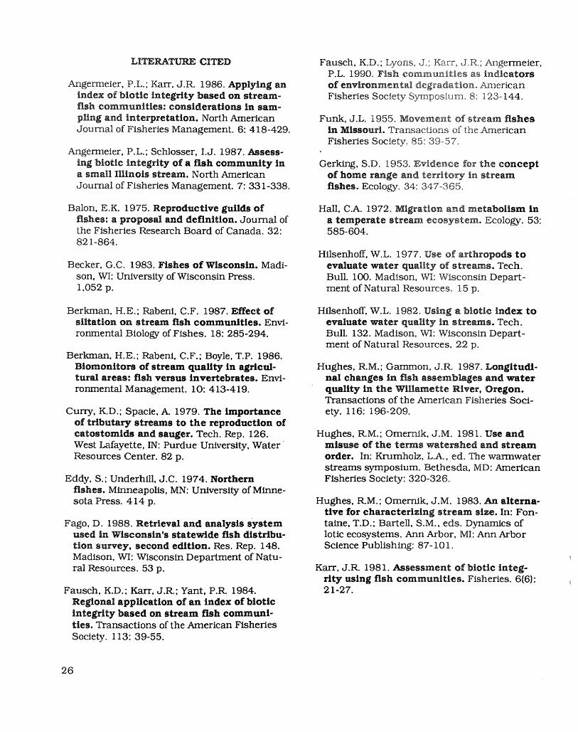
LITERATURE CITED Fausch, K.D.; Lyons, J.; Kary, J.R.; Angermeier,P.L. 1990. Fish communities as indicators

AngerTneier, P.L.; Karr, J.R. 1986. Applying an of environmental degradatioa, A_lericanindex of biotic integrity based on stream- Fisheries Society Symposium. 8: 123-144.fish communities: considerations in sam-

piing and interpretation. North American Funk, J.L. 1955. Movement of stream fishesJournal of Fisheries Management. 6: 418-429. in Missouri. Transactions of the American

Fisheries Society. 85: 39-57.Angermeier, P.L.; Schlosser, I.J. 1987. Assess-

ing biotic integrity of a fish community in Gerking, S.D. 1953. Evidence for the concepta smaU Illinois stream. North American of home range and territory in streamJournal of Fisheries Management. 7:331-338. fishes. Ecology. 34: 347-365.

Balon, E.K. 1975. Reproductive guilds of Hall, C.A. 1972. Migration and metabolism infishes: a proposal and definition. Journal of a temperate stream ecosystem, Ecology. 53:the Fisheries Research Board of Canada. 32: 585-604.821-864.

Hilsenhoff, W.L. 1977. Use of arthropods toBecker, G.C. 1983. Fishes of Wisconsin. Madi- evaluate water quality of streams, Tech.

son, WI: University of Wisconsin Press. Bull. 100. Madison, WI: Wisconsin Depart-1,052 p. merit of Natural Resources. 15 p.

Berkman, H.E.; Rabeni, C.F. 1987. Effecl of Hilsenhoff, W.L. 1982. Using a biotic index tosiltation on stream fish communities. Envi- evaluate water quality in streams. Tech.ronmental Biology of Fishes. 18: 285-294. Bull. 132. Madison, WI: Wisconsin Depart-

ment of Natural Resources. 22 p.

Berkman, H.E.; Rabent, C.F.; Boyle, T.P. 1986.Biomonitors of stream quality in agricul- Hughes, R.M.; Gammon, J.R. 1987. Longitudi-rural areas: fish versus invertebrates. Envi- hal changes in fish asserablages and waterronmental Management. I0:413-419. quality in the Willamette River, Oregon.

Transactions of the American Fisheries Soct-

Curry, K.D.; Spacte, A. 1979. The importance ety. 116: 196-209.of tributary streams to the reproduction ofcatostomids and sauger. Tech. Rep. 126. Hughes, R.M.; Omerntk, J.M. 1981. Use andWest Lafayette, IN: Purdue University, Water misuse of the terms watershed and s/reamResources Center. 82 p. order. In: Krumholz, L.A., ed. The warmwater

streams symposium. Bethesda, MD: AmericanEddy, S.; Underhfll, J.C. 1974. Northern Fisheries Society: 320-326.

fishes. Minneapolis, MN: University of Minne-sota Press. 414 p. Hughes, R.M.; Omernlk, J.M. 1983. An alterna-

tive for characterizing stream size. In: Fon-Fago, D. 1988. Retrieval and analysis system taine, T.D.; Bartell, S.M., eds. Dynamics of

used in Wisconsin's statewide fish distribu- lotic ecosystems. Ann Arbor, MI: Ann Arbortion survey, second edition, ires. Rep. 148. Science Publishing: 87-101.Madison, WI: Wisconsin Department of Natu-ral Resources. 53 p. Karr, J.R. 1981. Assessmenl of biotic integ-

rity using fish communities. Fisheries. 6(6):Fausch, K.D.; Karr, J.R.; Yant, P.R. 1984. 21-27.

Regional application of an index of bioticintegrity based on stream fish communi-ties, Transactions of the American Fisheries

Society. 113: 39-55.

26

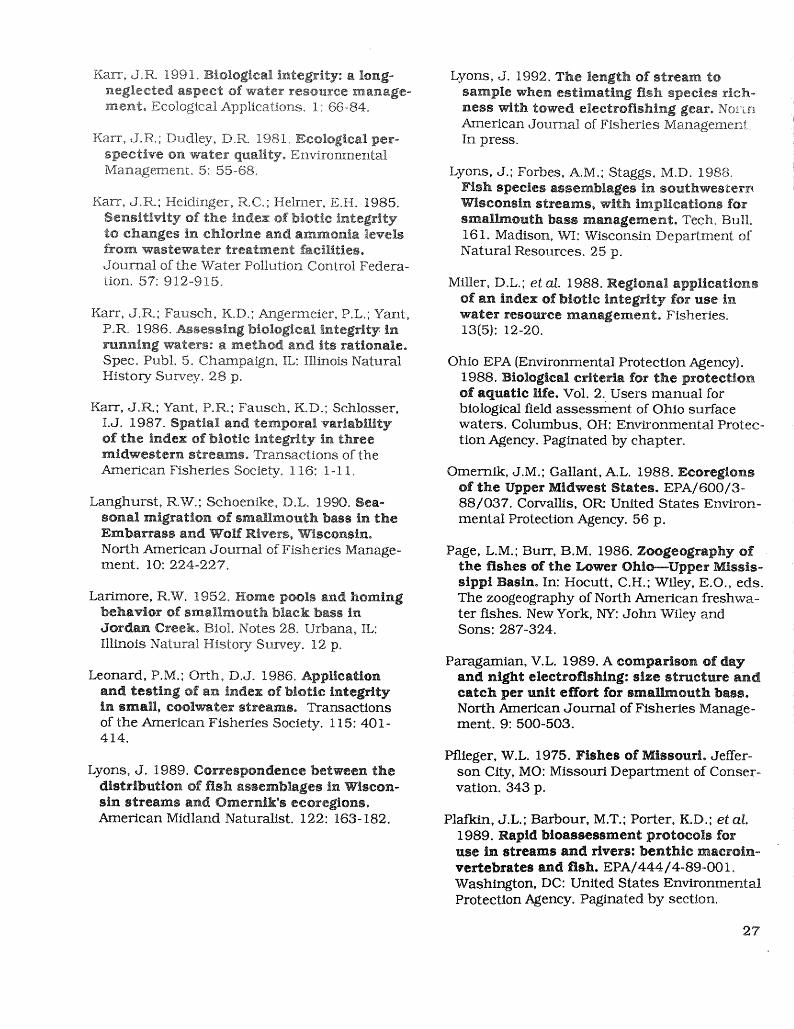
Karr, J. R, 1991, Biological integrity: a long- Lyons, J. 1992, The length of stream toneglected aspect of water resource manage- sample when estimating fish species rich-mento Ecological Applications. 1: 66-84. hess with towed electroflshing gear, Nol_r_

American Journal of Fisheries ManagementKarr0 J.R.; Dudley, D.R. 1981. Ecological per- In press.

speetive on water qaalityo Envtromnental

Management. 5: 55-68. Lyons, d.; Forbes, A.M.; Staggs, M.D. 1988,Fish species assemblages in southwestern

Karro J.R.; HeidiiNer, R.C.; Helmet, E.H. 1985. Wisconsin streams, with implications forSensttiviW of the index of biotic integrity smallmouth bass management, Tech. Bull.to changes in chlorine and ammonia levels 161. Madison, WI: Wisconsin Department offrom wastewater treatment faeilitieso Natural Resources. 25 p.Journal of the Water Pollution Control Federa-

tion. 57:912-9 t5. Miller, D.L.; et al. 1988. Regional applicationsof an index of biotic integrity for use in

Karr, J.R.; Fausch, K.D.; Ange_Tneier, P.L.; Yant, water resource management, Fisheries.P.R. 1986, A_sessing biological integrity in 13(5): 12-20.running waters: a method and its rationale.

Spec. Publ. 5. Champaign, IL: Illinois Natural Ohio EPA {Environmental Protection Agency).History Survey. 28 p. 1988. Biological criteria for the protection

of aquatic life, Vol. 2. Users manual forKarr, J.R.; YanL P°R.; Fausch, K.D.; Schlosser, biological field assessment of Ohio surface

I.J. 1987. Spatial and temporal 'variability waters. Columbus, OH: Environmental Protec-of the index of biotic integrity in three tion Agency. Paginated by chapter.midwestern streams° Transactions of the

.American Fisheries Society. 116:1-11. Omernik, J.M.; Gallant, A.L. 1988. Ecoregtonsof the Upper Midwest States. EPA/600/3-

Langhurst, R.W.; Schoenike, D.L. 1990, Sea- 88/037. Corvallis, OR: United States Environ-

sonal migration of smallmouth bass in the mental Protection Agency. 56 p.Embarrass and Woff Rivers, Wisconsin.

North American Journal of Fisheries Manage- Page, L.M.; Burr, B.M. 1986. Zoogeography ofmerit. 10: 224-227. the fishes of the Lower Ohio--Upper Missis-

stppi Basin, In: Hocutt, C.H.; Wiley, E.O., eds.Larimore, R.W. t952. Home pools and homing The zoogeography of North American freshwa-

behavior of smallraouth black bass in ter fishes. New York, NY: John Wiley andJordan Creek, Biol. Notes 28. Urbana, IL: Sons: 287-324.

Illinois Natural History Survey. 12 p.

Paragamian, V.L. 1989. A comparison of dayLeonard, P.M.; Ortho D.J. 1986. Application and night electrofishtng: size structure and

and testing of an index of biotic integrity catch per unit effort for smallraouth bass.in small, coolwater streams, Transactions North American Journal of Fisheries Manage-of the American Fisheries Society. 115: 401- merit. 9: 500-503.414.

Pflleger, W.L. 1975. Fishes of Missouri, Jeffer-Lyons, J. 1989. Correspondence between the son City, MO: Missouri Department of Conser-

distrlbntton of fish assemblages in Wtscon- vation. 343 p.sin streams and Omernik's ecoregions,American Midland Naturalist. 122: 163-182. Plaikin, J.L.; Barbour, M.T.; Porter, K.D.; et al.

1989. Rapid btoassessment protocols foruse in streams arid rivers: benthic macroin-

vertebrates and fish. EPA/444/4-89-001.

Washington, DC: United States EnvironmentalProtection Agency. Paginated by section.

27

Rankln, E.T.; Yoder, C.O. 11990. The nature of Schlosser, I.J.: Ebeto K.K. 1989. Effects of flow

sampling variability in the Index of Biotic regime and cyprinid predation on a head-Integrity (IBI) in Ohio streams, In: Da_s, water stream. Ecological Monographs. 59:WLS., ed. Proceedings of the 1990 Midwest 41-57.pollution control biologists meeting. EPA/905/9-90-005. Chicago, IL: United States En- Smith, P.W. 1979. Fishes of Illinois° Cham-vironmental Protection Agency Region 5, Envi- palgn, IL: University of Illinois Press. 314 p.ronmental Sciences Division: 9-18.

Steedman, R.J. 1988. Modification and assess-

Revak, C. 1989. Analysis of the order system ment of an Index of Biotic Integrity toacross Wisconsin's different geographic re- quantify stream quality in southern On-gions. Scientific Wisconsin (University of ratio. Canadian Journal of Fisheries andWisconsin-Stevens Point). 2(1): 1-10. Aquatic Sciences. 45:492-501.

Robins, C.R.; Bailey, R.M.; Bond, C.E.; et al. Trautman, M.B. 1981. The fishes of Ohio.1991. Common and scientific names of Columbus, OH: The Ohio State Universityfishes from the United States and Canada. Press. 782 p.

5th ed. Spec. Publ. 20. Bethesda, MD: Ameri-can Fisheries Society. 183 p. Underhill, J.C. 1986. The fish fauna of the

Laurenflan Great Lakes, the St. Lawrence

Schlosser, I.J. 1990. Environmental variation, Lowlands, Newfoundland, and Labrador. In:

life history attributes, and community Hocutt, C.H.; Wiley, E.O., eds. The zoogeogra-structure in stream fishes: implications for phy of North American freshwater fishes. Newenvironmental management and assess- York, NY: John Wiley and Sons: 105-136.ment. Environmental Management. 14:621-628.

28

APPENDIX 1

DE*,K_L_P_'T _D VALIDATION OF THE I evaluated and developed scoring criteria forWISCONS_ VERSION fish community composition and relative abun-

dance metrics (metrics based on counts of

Development individual fish; i.e., species composition, trophicand reproductive function, m-ld fish abundance

The Wisconsin IBI was developed using a large and condition metrics) wlth data collected

aznount of fish community data, in some cases during 1987 through 1989 as part of a WDNR

coupled with habitat and water quality informa- research study that I directed. This studytion, from streams and rivers throughout the explored relationships between fish communi-State. Species richness metrics and MSR plots ties and physical habitat characteristics in

were based on data from the WDNR Fish Distri- WalTnwater streams throughout Wisconsin, andbution Survey (Fago 1988). From 1974 through encompassed streams ranging from very poor to1979, the Fish Distribution Survey sampled fish excellent in environmental quality. Completecommu_tles at more than 4,500 discrete fish community data, including counts of allstations on more than 1,700 lakes, rivers, and fish captured, were collected from 70 stations

streams throughout the southern and western on 39 streams. All fish data were collected bythirds of Wisconsin. From the survey data base, wading with a standard WDNR DC stream

I chose 490 stations on 290 warmwater streams shocker during June, July, or August.and rivers for development of MSR lines. At all

of these stations, survey personnel had at- Additionally, detailed physical habitat measure-

tempted to completely sample the entire fish ments (stream widths, depths, and discharge;community, and all captured fish were accu- water velocity, temperature, conductivity, and

rarely identified to species. However, counts of turbidity; bottom substrate composition; hidingfish within each species stopped at 99, so the cover for adult fish; pool-riffle development,data did not always adequately represent rela- channel gradient, and sinuosity; and banktire abundance of species. All stations had stability, riparian vegetation, and land use) were

been sampled by wading with either a standard made at each station during fish sampling.WDNR DC backpack electroshocker or stream Some of these measurements were used to

shocker during June, July, or August. An develop a 100-point rating scale for physicalestimate of mean stream width, which I used as habitat quality (fig. 13). Water quality was ratedmy measure of stream size, was available for on a four-point scale (table 8), using qualitativeeach station, observations made at the station coupled with

qualitative and quantitative water qualityTo develop MSR plots, I graphed the number of information from WDNR stream files.species versus the natural log of the mean

stream width in meters. I made separate plots I considered 15 possible fish community compo-for each of the three geographic areas and each sition, trophic and reproductive function, andof the five species richness metrics (totals of relative abundance _ind condition metrics for

native species, darters, sunfish, suckers, and inclusion in the IBI (see Appendix IV). These 15intolerant species) for a total of 15 plots. For included all of those from Karr's original versioneach plot I then drew the MSR line and derived (Karr 1981, Karr et al. 1986) and the Ohio EPA

scoring criteria (see Appendix 3). Stations with "wading sites" version (Ohio EPA 1988), plus aa species richness near or above the MSR line few from other versions of the IBI (Leonard andfor a particular metric received a score of 10 for Orth 1986, Miller et al. 1988, Steedman 1988).that metric. Stations with a species richness far For each potential metric, I correlated station

below the MSR line received a score of 0, and values for that metric with station ratings forstations with intermediate species richness habitat quality, water quality, and overallreceived intermediate scores, environmental quality (a composite index ob-

tained by multiplying the water quality rating bythe habitat quality rating and dividing by four).

29

II I ill I I I

WISCONSIN WAK_¢ATEK STREAM PHYSICAL HABITAT RATING FORM

Stream: Water Both/ [O:

Year: Month: Day: Entire Stre_ M_[e:

Evaluators: Total Score:

CATEGORY

Rating Item Excel lent Good Fair Poor Score

Bank erosion, No significant bank Limited amount of bank Intermediate amount Extensive amount of

faiture and erosion, failure, erosion, failure, of bank erosion, bank erosion, fail-bank protec- >_90% of bank pro- 80% of bank protected failure. 60% of ure. ! 50% of bank

lion. tected by plants by plants or stable bank protected by protected by plantsor stable rock. rock, plants or stab(e or stable rock.

rock.

12 8 4 0r

Main channel ->65% of the bottom 45% of the bottom 25% of the bottom _<5% of bottom

rocky covered by rocky covered by rocky covered by rocky covered by rockysubstrate substrate (BE + 30 substrate, substrata, substrate.

(% of area). + RC + GR).

25 16 8 0

Available Extensive cover, Adequate cover, 8% Cover limited, 4 % Little or no cover,cover for (woody debris, of the total surface of the total sur- 0% of the total sur-

adult rocks, or macro- area. face area. face area.

gamef _sh. phyte beds)> 12% of totalsurface area.

25 16 8 0

Average max- >_ 1.5 meters. 1.2 meters. 0.9 meters. _<0.6 meters.

imum Tha[weg

depth (4 deep- ii

est depths). 25 16 8 0 i

..... 4

BB or RR Ratio BB or RR Ratio _< 12. BB or RR ratio = 18. 8B or RR ratio = 24. BB or RR Ratio >_30.(distance be- l

tween bends or

riff les/avg.

main channel

width). 12 8 4 0

99 = Excellent 66 = Good 33 = Fair 0 = Poor Total Score:

Figure 13.--Criteria and example of data sheet used to rate physical habitat quality at sites sampledd_'ing 1987-1990. The four categories (Excellent, Good, Fair', Poor) are provided as guidelines; theactual scores for each rating item can be fnbetween the scores given for two adjacent categories.Terms and abbreviations used on the form include:

Water Body _a unique seven-digit identification code assigned to each stream, river, and lakein Wisconsin.

Entire Stream Mile---The distance in miles (via the stream channel) between the mouth of thestream and the downstream end of the site. Used to indicate site location on the stream.

Main Chan_el Rocky Substrata--BE = Bedrock, BO = Boulder, RC = Rubble�Cobble, GR =Gravel.

BB or RJFtRatio---Bend to Bend or Riffle to R_le Ratio,

30

Table 8 o--Crtterta for assigning water gualtty ratings to sites sampled in 1987-1990

Score Rating Criteria

1 Very poor Major fish kill within I year, or a history of regular fish kills, or chronic (more than once peryear) severe violations of Wisconsin standards for key water quality characteristics (e.g.,dissolved oxygen, pH, suspended solids, ammonia, nitrates, pesticides, heavy metals).

2 Poor Major fish kill within 5 years, or occasional (less than once per year) severe violations of Wis-consin standards for key water qua]ity characteristics.

3 Fair No known fish kills within 5 years, but site either is located in critical non-point source pollutionwatershed or highly developed urban or suburban area where poor quality runoff is possible,or occasionally suffers from minor violations of Wisconsin standards for key water qualitycharacteristics.

4 Good No evidence of fish kills or vioJatiansof Wisconsin standardsfor key water quality characteris-tics. Site located in an area where poor quality runoff is unlikely.

ASSF.SSMIt, N_£0_" POTENTIAL _TRICS Table 9.--Correlations (Spearman's Rank Correla-tion Coefficient) between potential metrics and

I selected metrics for the Wisconsin version of an independent measure of environmentalthe IBI based on the magnitude of their correla- quality for the 70 sites sampled during 1987-tion with environmental quality and their appro- 1989priateness for use in all parts of the State.Using these criteria, I chose to retain the follow- Correlation Significanceing metrics, all of which are also used in the Potential metric coefficient (r) value (p)Ohio EPA {1988) "wading sites" version of theIBI: Percent green sunfish -0.50 0.0001

Percent tolerant species -0.57 0.0001Percent tolerant species Percent common carp -0.45 0.0001Percent omnivores Percent creek chub 0.16 0.1934Percent insectivores Percent white sucker -0.32 0.0070Percent top carnivores Percent omnivores -0.50 0.0001Percent simple lithophilous spawners Percent facultative omnivores -0.01 0.9476

Percent generalist feeders 0.16 0.1921I also retained two other metrics as correction Percent insectivorous Cyprinids 0.17 0.1543factors: Percent insectivores 0.32 0.0064

Percent top carnivores 0.58 0.0001Number of individuals (excluding tolerant Percent hybrids -0.29 0.0157

species) per 300 m sampled Percent simple lithophilousPercent DELT (deformed, eroded fins, lesions, spawners 0.25 0.0372

tumors) fish Number of individualsper 300 msampled 0.15 0.2096

Number of individuals, or Its equivalent, has Percent DELT fish -0.15 0.2084been used in most other versions of the IBI(Karr et al. 1986, Miller et al. 1988, Ohio EPA1988). I did not find a strong relationshipbetween number of individuals and environ-

mental quality (table 9), although the lowest

3i

1600 Ii

= _ 1987-1989 Data1400 F

P-- 1200

"_ 1000"5

800 -

_ 4o0

•.; 200:S=

m 0 -- ..............

POOR FAIR GOOD EXCELLENT

Environmental Quality Rating

Figure 14.--Plot of rnean catch of individuals per 300 m sampled (excZud-ing tolerant species)for four levels of the Environmental Quality Rating°The Poor rating was given to sites with environmentat quality scoresfrom 0 to 24, the Fair rating was given to sites with scores from 25 to49, the Good r&ting was given to sites with scores from 50 to 74, andthe Excellent rating was given to sites with scores from 75 to 100.Lines bisecting the bars indicate the 95 percent confidence limits of themearu

numbers occurred at the sites with the worst grossly polluted sites (Karr et at. 1988, Ohio

environmental quality (fig 14; ANOVA and Bon- EPA 1988). Only a few such sites were sampledferronl Multiple Comparisons Test of log(Catch + during 1987-1989, so I have retained percentI); F = 7.15, p = 0.0003). The highest numbers DELT fish as a correction factor that onlyoccurred at sites with fair environmental qual- influences the overall IBI score when the pro-ity. Therefore, the number of individuals portion of DELT fish is high.correction factor only influences the overall IBI

score when the number of individuals is very I rejected the following eight metrics:low.

Percent common ca_>---Common carp (Cyp-Percent DELT fish has also been used in most rinus carplo) relative abundance tends to in-

other versions of the IBI (Karr et al. 1986, Miller crease with increasing environmental degra-et al. 1988, Ohio EPA 1988). However, very few dation (Karr et al. 1986, Miller et al. 1988).

DELT fish were encountered in Wisconsin However, carp reach the northern edge ofduring the 1987-1989 sampling. Of 70 sites, 24 their range in Wisconsin and are rare In

had DELl" fish, but no site had more than four, northern Wisconsin (Becket 1983). They alsoand the maximum percentage was 0.5 percent, do not occur in high abundance in high

There was not a significant relationship between gradient streams (Lyons 1989). Althoughrelative abundance of DELT fish and environ- percent common carp was negatively corre-mental quality [table 9). However, other studies fated with environmental quality, the percent

have found high numbers of DELT fish at tolerant species metric (of which carp forma part) had a better correlation {table 9).

32

Percent creek ehu_--Creek chub relative

abundance is often high at degraded sites Percent insectivorous cyprinids--tnsectivo-(Karr et aL 1986, Leonard and Orth t986), rous cyprirAds tend to decline as environ-However, creek chubs usually do best in mentat degradation increases (Kan- et at.small streams and tend to be uncommon in 1986). However, they are naturally rare Inlarger streams (Becker 1983)o Percent creek very low gradient streams (Lyons, unpub-chub was not correlated with environmental llshed data). Addittonally, the relative abun-quality (table 9). dance of insectivorous cyprinids was not

correlated with environmental quality (tablePercent green sunfishwGreen sunfish rela- 9).rive abundance tends to increase with in-

creasing environmental degradation (Karr et Percent hybrids-Hybrids are often commona/. 1986). However, green sunfish reach the at degraded sites. However, hybrids arenorthern edge of their range in Wisconsin difficult to identify, and they were rare in theand are rare in northern Wisconsin (Becker 1987-1989 data set.1983). They also do best in small streamsand tend to be uncommon In larger streams Scoring criteria for the five metrics chosen for(Ohio EPA 1988). Although, percent green inclusion in the Wisconsin IBI were based onsunfish was negatively correlated with the distribution of station values for eachenvironmental quality, the percent tolerant metric. The four stations (5.7 percent of total)species metric (of which green sunfish form with the best values for each metric (highest ora part) had a better correlation (table 9). lowest values, depending on the nature of the

metric) determined the expected value forPercent white sucker--White sucker (Ca- streams with good environmental quality.tostomus commersoni ) relative abundance is Stations with metric values near this expectedoften high at degraded sites (Karr et at. 1986; value scored a 10 for that metric. Stations withMiller et at. 1988). Although, percent white metric values much worse than the expectedsucker was negatively correlated with envl- value scored a 0, and stations with intermediateronmental quality, the percent tolerant values received an intermediate score.species metric (of which white suckers forma part) had a better correlation (table 9). Other versions of the IBI rate metrics on a

scoring scale from 1 (worst) to 5 (best) (Karr etPercent facultatlve omntvores--Under a/. 1986, Leonard and Orth 1986, Miller et al.certain degraded conditions, normally inset- 1988, Steedman 1988). Most of these othertivorous common shiners (Luxilus cornutus) versions have 12 metrics, resulting in a possibleand spoffin shiners (CyprineUa spiloptera) range of IBI values from 12 (worst) to 60 (best).may have an omnivorous diet (Ohio EPA Wisconsin biologists unfamiliar with the IBI1988). However, the combined relative tend to not like this scoring range, and severalabundance Of these two species was not of them requested that the Wisconsin versioncorrelated with environmental quality (table have a more easily interpretable scale (personal9). observations). Thus, I have scaled the Wiscon-

sin IBI from 0 to 100, scoring each metric over aPercent generalist feeders--Creek chubs range of 0 to 10.and blacknose dace have vaned, broad diets,

and often respond positively to environmental Validationdegradation and food web disruption in thesame manner as omnivores (Leonard and To validate whether the Wisconsin IBI trulyOrth 1986, Ohio EPA 1988, Steedman 1988). reflected the environmental quality of a stream,However, the combined relative abundance of I tested whether there was a significant positivethese two species was not correlated with relationship between the overall IBI score andenvironmental quality (table 9). independent measures of environmental quality.

33

I ilHllllIlHIINII'

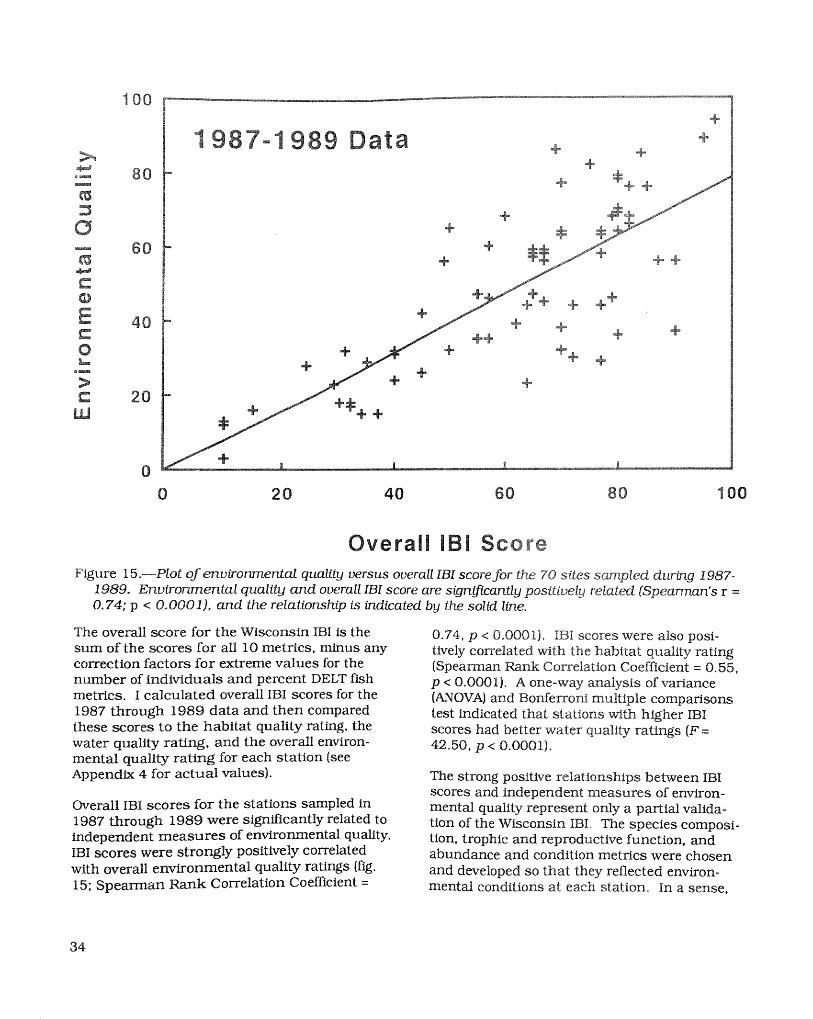
100 ['_

+

87-1 989 Data + + ++

°_ 80 + #+ +_3c_ + @o

&_ +o +++ + ++E 40 + + + +E ++ ,+O + + ++

> + + +,E 20

+ +uJ #

Overall iSi Score

Figure 15.--Plot of envirormlentat quality versus overall IBf score for the 70 sites sampled during I987-I989. Environmental quality and overall IBI score are significantly positively related (Spearman's r =0.74; p < 0.0001), and the relationship is indicated by the solid line.

The overall score for the Wisconsin IBI Is the 0.74, p < 0.0001). IBI scores were also posi-sum of the scores for all 10 metrics, minus any tively correlated with the habitat quality ratingcorrection factors for extreme values for the (Spearman Rank Correlation Coefficient = 0.55,number of individuals and percent DELT fish p < 0.0001). A one-way analysis of variancemetrics. I calculated overall IBI scores for the (ANOVA) and BonfeFroni multiple comparisons1987 through 1989 data and then compared test indicated that stations with higher IBIthese scores to the habitat quality rating, the scores had better water quality ratings {F =water quality rating, and the overall environ- 42.50, p < 0.0001).•mental quality rating for each station (see

Appendix 4 for actual values). The strong positive relationships between IBIscores and Independent measures of environ-

Overall IBI scores for the stations sampled In mental quality represent only a partial vallda-

1987 through 1989 were significantly related to tion of the Wisconsin IBI. The species composi-Independent measures of environmental quality, tlon, trophic and reproductive function, andIBI scores were strongly positively correlated abundance and condition metrics were chosen

with overall environmental quality ratings (fig. and developed so that they reflected environ-15; Spearman Rank Correlation Coefficient = mental conditions at each station. In a sense,

34

100

1990 Data>_

80 °+

t_

= ++©

,,_ 60 ° + +fi:

E 4o

C: + + +0&>

2O

UJ ++ +++

0 20 40 60 80 100

Overall IBI ScoreFigure 1&--Plot of envfronmentat quality versus overall IBI score for the 28 sites sampled during 1990.

Environmental quality and overall ZBZscore are significantly positively related (Spearman's r = 0.60; p= 0.0007), and the relationship ts indicated by the solid line.

the IBI was developed to mimic patterns of envl- Analysis of 1990 data validated the Wisconsinronmentat quality at a specific set of stations, version of the IBI. Overall IBI scores were againDetemUnmg whether IBI scores were likely to strongly positively correlated with overall envl-reflect environmental quality at other stations ronmental quality ratings (fig. 16; Spearmanrequired an independent test using data from a Rank Correlation Coefficient = 0.60, p =new set of stations. 0.0007). IBI scores were also positively corre-

lated with the habitat quality rating, althoughI carried out this test with data from 1990. The the correlation was only marginally significantresearch study that produced the 1987-1989 (Spearman Rank Correlation Coefficient = 0.31,data continued into 1990, with data collected in p = 0. I071). The weaker relationship betweenthe same manner as previously. In 1990, a IBI scores and habitat ratings occurred becausetotal of 28 stations on 16 streams were three of the 1990 stations had fair to good

sampled. Seven of these stations on four habitat but very poor water quality and hencestreams had also been sampled during 1987- very low IBI scores. A one-way ANOVA and1989, but the rest were sampled for the first Bonferronl multiple comparisons test againtime. I related IBI scores to environmental indicated that stations with higher IBI scores i

quality ratings for the 1990 set of stations, had better water quality ratings (F= 8.17, p = !_o.ooo6), i

ii

35 !

!

:i

Table I O.--IBI and environmental quality data for sites sampled duFtng 1987-t989; higherscores Lndlcate better quality

Stream County Ml_e1 tBF EQ3 HOff WQ5

Amnicon R. Douglas 5.7 80 69 69 4Big Plover R. Portage 7.4 80 70 70 4Big Plover R. Portage 8.8 80 64 64 4Big Rib R. Marathon 13.1 64 44 59 3Big Rib R. Marathon 14.7 82 66 66 4Big Rib R. Marathon 16.5 77 63 63 4Big Rib R. Marathon 17.9 50 32 32 4Big Rib R. Marathon 18.0 77 58 58 4Big Rib R. Marathon 19.0 79 68 68 4Big Roche a Cri Cr. Adams 2.0 77 64 64 4Big Roche a Cri Cr. Adams 6.8 50 65 65 4CedarCr. Washington 18.5 45 26 34 3Cedar Cr. Washington 19.4 37 15 20 3Crawfish R. Dodge 37.8 57 35 47 3Crawfish R. Dodge 38.7 45 42 56 3Crawfish R. Dodge 39.6 79 46 61 3East Fork Chippewa R. Ashland 24.1 80 79 79 4East R. Brown 10.6 10 12 24 2Embarrass R. Shawano 46.6 84 85 85 4Galena R. Lafayette 29.8 29 23 45 2Goose Lake Canal Racine 2.4 10 3 5 2Hay R. Dunn 16.6 67 59 78 3Jump R. Rusk 3.5 95 89 89 4Jump R. Rusk 7.2 82 76 76 4Little Platte R. Grant 19.4 35 29 57 2LittleWolf R. Waupaca 9.9 85 76 76 4LivingstonBr. iowa 2.5 32 18 36 2Manitowish R. Vilas 31.4 65 58 58 4Mecan R. Marquette 9.5 49 56 56 4Menominee Cr. Grant 7.7 40 31 62 2Menomonee R. Milwaukee 3.0 15 16 64 1Menomonee R. Milwaukee 5.7 10 13 50 1MilwaukeeR. Ozaukee 53.4 65 47 63 3Milwaukee R. (1988) Washington 64.6 55 35 47 3MilwaukeeR. (1989) Washington 64.6 57 46 61 3Milwaukee R. (1988) Washington 65.5 30 18 24 3MilwaukeeR. (1989) Washington 65.5 40 32 42 3Milwaukee R. Washington 66.0 24 28 37 3Milwaukee R. (1988) Washington 66.8 62 39 52 3Milwaukee R. (1989) Washington 66.8 55 47 63 3Mineral Point Br. Iowa 12.6 64 23 30 3Mineral Point Br. Iowa 13.0 72 44 59 3Moose R. Douglas 1.0 70 63 63 4Moose R. Sawyer 2.5 67 58 58 4Mukwonago R. Waukesha 1.3 80 36 36 4

(Table 10 continued on next page)

36

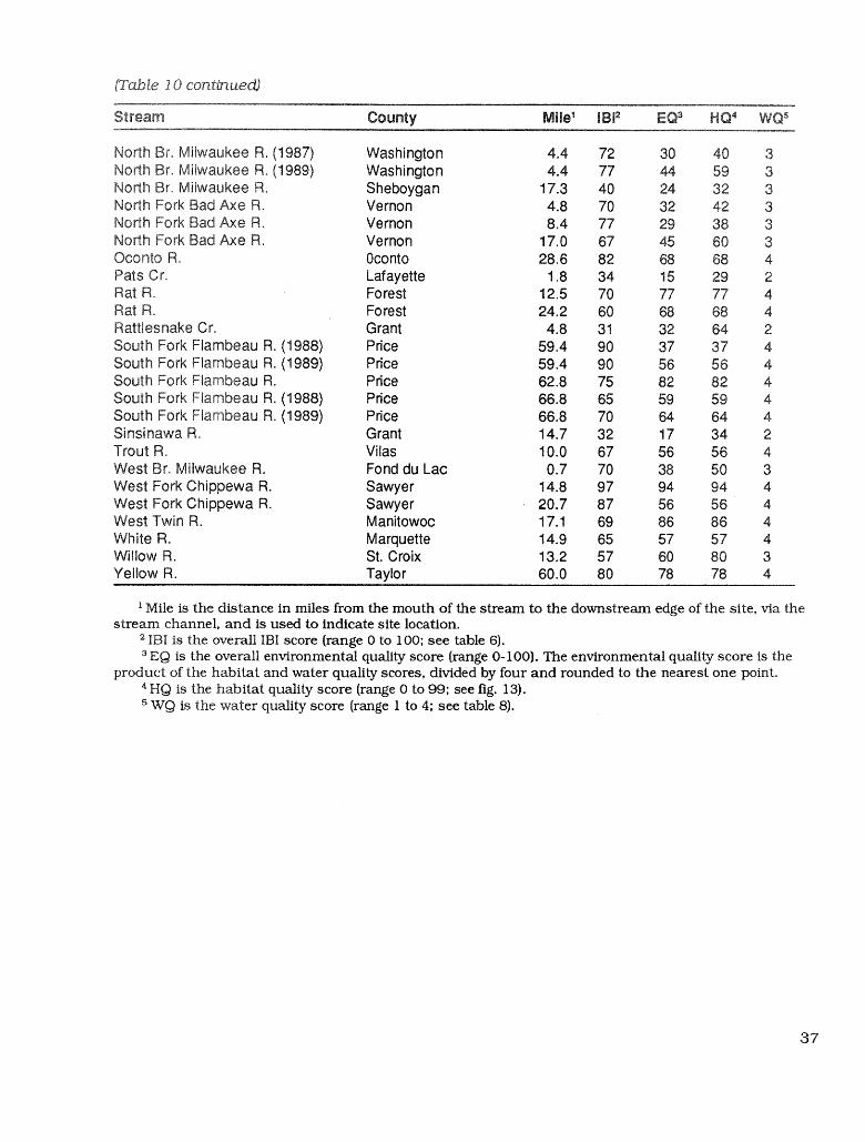
(Table 10 contfnued)

Stream County Mile 1 18F EQ3 HQ 4 W@

North Br. Milwaukee R. (1987) Washington 4.4 72 30 40 3North Br. Milwaukee R. (1989) Washington 4.4 77 44 59 3North Br. Milwaukee R. Sheboygan 17.3 40 24 32 3North Fork Bad Axe R. Vernon 4.8 70 32 42 3North Fork Bad Axe R. Vernon 8.4 77 29 38 3North Fork Bad Axe R. Vernon 17.0 67 45 60 3Oconto R, 0conto 28.6 82 68 68 4Pats Cr. Lafayette 1.8 34 15 29 2Rat R. Forest 12.5 70 77 77 4Rat R_ Forest 24.2 60 68 68 4Rattlesnake Cr. Grant 4.8 31 32 64 2South Fork Flambeau R. (1988) Price 59.4 90 37 37 4South Fork Flambeau R. (1989) Price 59.4 90 56 56 4South Fork Flambeau R. Price 62.8 75 82 82 4South Fork Flambeau R. (1988) Price 66.8 65 59 59 4South Fork Flambeau R. (1989) Price 66.8 70 64 64 4Sinsinawa R. Grant 14.7 32 17 34 2Trout R. Vilas 10.0 67 56 56 4West Br. Milwaukee R. Fond du Lac 0.7 70 38 50 3West Fork Chippewa R. Sawyer 14.8 97 94 94 4West Fork Chippewa R. Sawyer 20.7 87 56 56 4West Twin R. Manitowoc 17.1 69 86 86 4White R. Marquette 14.9 65 57 57 4Willow R. St. Croix 13.2 57 60 80 3Yellow R. Taylor 60.0 80 78 78 4

1Mile is the distance in miles from the mouth of the stream to the downstream edge of the site, via thestream channel, and Is used to Indicate site location.

2IBI is the overall IBI score {range 0 to 100; see table 6).3EQ is the overall environmental quality score (range 0-100). The environmental quality score is the

product of the habitat and water quality scores, divided by four and rounded to the nearest one point.4HQ is the habitat quality score (range 0 to 99; see fig. 13).5 WQ is the water quality score (range 1 to 4; see table 8).

37

Table 11 .--IBt and environmental quality data for sites sampled durlng t 990° (Seelegend from table 1Of or explanations of column headings).

Stream County Mite tBt EQ HQ WQ

Beaver Dam R. Dodge 18.9 0 10 41 1Beaver Dam FI. Dodge 20,2 0 16 65 1Beaver Dam R. Dodge 26,5 24 16 65 1Little Platte R. Grant 19,4 .37 38 71 2Manitowish R. iron 11.3 80 77 77 4MiJwaukeeR. Washington 64.6 12 52 69 3Milwaukee R. Washington 85.5 24 48 64 3Milwaukee R. Washington 68.8 50 59 79 3Mineral Point Br. Iowa 12,6 80 29 39 3North Br. MiJwaukeeR. Washington 4.4 60 46 61 3North Br. Pike R. Kenosha 0.9 2 16 63 1North Br. Pike R, Racine 2,8 27 9 37 1North Br. Pike R. Racine 3.8 30 8 30 1North Fork Eau Claire R, Eau Claire 11.5 60 48 48 4Otter Or, Lafayette 4.1 50 34 67 2Otter Or, Lafayette 6.6 42 28 55 2Pike R. Kenosha 2.6 5 21 42 2Pike R, Kenosha 5.9 30 29 57 2Pike R, Kenosha 8.3 15 31 62 2South Br. Pike R, Kenosha 0.5 27 26 52 2South Br, Pike R. Kenosha 2.4 25 12 24 2South Fork Eau Claire R, Eau Claire 24.6 69 70 70 4Squirrel R. Oneida 6.7 55 49 65 3Tomahawk R. Oneida 43.6 75 57 76 3Tomahawk R. Oneida 53.6 75 43 57 3Waumandee Cr. Buffalo 17.1 19 35 47 3Waumandee Cr. Buffalo 21,0 22 14 19 3Wisconsin R. Vilas 406.6 70 68 68 4

38

WHERE NOT TO USE THIS VERSION picture of the fish community in larger streams.OF THE IBI The difficulty in applying the IBI lies in combin-

ing the sampling results from these differentVery Small Warmwater Streams methods. Each sampling method has different

biases and capture efficiencies, and sknplyThe nature of fish communities in very small adding together catches from different samplingwarmwater streams (intermittent and/or <2.5 m techniques and gear types is usually lnappropri-wide) differs substantially from that of fish ate. It may be possible to formulate samplingcommunities in larger warmwater streams, so protocols that involve standardized units ofversions of the IBI developed for intermediate- effort for combinations of methods, but this hassized streams are inappropriate for very small not yet been done. The Ohio EPA (1988) hasstreams. In Wisconsin, very small warmwater developed a version of the IBI for larger Ohiostreams are often harsh, highly variable envi- rivers (their "boat" sites version) based solely onronments, even in the absence of human per- boat electroflshing, but it is not known how thisturbation. As a result, their fish communities version will work on larger warmwater streamsare usually dominated by a small number of' and rivers in Wisconsin.small, mobile, generalist or tolerant speciessuch as the bigmouth shiner {Notropis dorsalis), Coldwater and Coolwater Streamscreek chub, fathead minnow (PimephalespromeIas), blacknose dace, and green sunfish In Wisconsin, coldwater streams have maximum(Lepomis cyanetlus) (Lyons et aL 1988, Lyons daffy summer temperatures that rarely exceed1989). Because these opportunistic species 22°C, and coolwater streams have maximummove in and out of small warmwater streams as daffy summer temperatures that rarely exceedphysical and chemical conditions change, 24°C. Summer water temperatures in warmwa-natural variability in fish community structure ter streams regularly surpass these levels. I doand function tends to be high. This natural not believe that tt will be possible to develop avariability makes It difficult to develop an version of the IBI that will be effective foreffective version of the IBI for very small warm- coldwater and coolwater streams In Wisconsinwater streams. The Ohio EPA (1988) has devel- without fundamental changes in the index.oped a version of the IBI for very small warmwa- This is because the response of Wisconsinter streams in Ohio (their "headwater sites" coldwater and coolwater streams to many typesversion), but thls version has not yet been of degradation violates one of the key underlyingtested in Wisconsin. assumptions of the Wisconsin IBI and all other

versions of the IBI proposed thus far. All cur-Large Warmwater Streams and Rivers rent versions of the IBI are based on the as-

sumption that as environmental degradation in-Warmwater streams and rivers too large to creases and biotic integrity declines, the num-sample effectively by wading require a different ber of species declines. In Wisconsin coldwaterversion of the IBI than intermedlate-sized and coolwater streams, moderate levels ofwarmwater streams. Electroshocking by wading environmental degradation often result incannot effectively sample all areas of large Increased species richness, and species rich-streams and rivers, so large streams and rivers ness often declines as environmental qualityrequire a more complex sampling scheme than and biotic integrity improve.intermediate-sized streams. Usually thisscheme involves a combination of sampling For example, consider the case of Timber Couleetechniques and gears (boat electrofishing, gill/ Creek in west-central Wisconsin. During thetrammel netting, trap netting, and/or trawling 1960's, poor agricultural land use practices andin deeper areas; wading electrofishing and/or bank erosion caused biotic integrity in theseining in shallow areas) because no one tech- stream to decline. Once a good coldwater troutnique alone can give a reasonably complete

39

stream, habitat in the Timber Coulee Creek had and coldwater streams. Relatively few W°lscon -

been so degraded that only heavy stocking sin fish species can persist in coolwater andpermitted trout to persist there. Beginning In coldwater streams, but many can persist inthe late 1960's, the WDNR undertook a massive warmwater streams. Thus, high quality coolwa-

habitat improvement project over several kilo- ter and coldwater streams tend to have lowermeters of the stream. Riparian land-use prac- species richness than comparably sized warm_tices were improved, banks were stabilized, and water streams. Small coldwater streams some-

Instream habitat was greatly enhanced. Biotic times contain only one or two species {a troutintegrity improved greatly, and the stream now and a sculpin or a Rhintchthys species).supports a healthy trout population with manylarge individuals. Stocking is no longer needed Most types of environmental degradation lead toto maintain this population. However, as a Increased maximum summer water tempera-consequence of habitat improvement, species tures. For example, poor land-use practicesrichness in Timber Coulee Creek declined by and increased erosion often result in a reduc-one to six species (8 to 67 percent) depending tion of cold groundwater or spring inputs toon location (fig. 17). Improved biotic integrity streams, removal of riparian vegetation andresulted in reduced species richness, decreased shading of streams, and wider,

shallower stream channels that more effectivelyWhy do eool/coldwater streams and warmwater absorb solar radiation. As streams become

streams respond differently to changes In biotic degraded, summer water temperatures willintegrity?. The answer to this question lles in often increase enough to permit colonization bythe temperature preferences of Wisconsin fishes warmwater species. Even if water temperaturesand the relationship between environmental increase to the point where coolwater or coldwa-degradation and water temperature in coolwater ter species are eliminated, a greater number of

warmwater species will probably be able to taketheir place. Thus, species richness will increase

is ...........................................................................................................................................................................even though environmental quality, and with it; Timber Coulee Creek "

14 . v_,,r.... c....ty._v_ biotic integrity, have declined.

12Some coolwater and coldwater streams are

.lo i degraded to the point where they have become_ warmwater streams. With improvements ins

"'_ environmental quality, these streams mightE 6, again become coolwater or coldwater and de-

4 .. A,,o,,n,..........,_-,. cline in species richness. As presently formu-lated, the IBI may not be the most appropriate

2 _

tool for assessing biotic integrity in theseo .............................................................................................................................................streams. But how can potential coolwater and

s z , 9 _o __ _2 _a _4 _s coldwater streams be identified?Distance Upstream from Mouth (km)

Coolwater and coldwater streams have charac-

Figure 17._Totat species richness at several teristic fish faunas. As these types of streamssites in Timber Coulee Creek, west-central become degraded, their fish faunas are joinedWisconsin, during two time periods. The and ultimately replaced by generalist anddownstream-most sites are to the left of the tolerant warmwater species. Moderately de-

plot, and the upstream-most are to the right, graded coolwater and coldwater streams usuallySites sampled in 1966, before habitat and have a mixed fish fauna, with some coldwater or

biotic integrity were improved, are indicated coolwater species and some warmwater species.by triangles and a solid line. Sites sampled By examining species composition, it may beafter habitat and biotic integrity were ira- possible to identify potential coolwater orproved are indicated by circles (1976), a coldwater streams that have been converted to

square (1980), and a dashed line. warmwater by environmental degradation.

40

/

t

Table 12 lists species generally restricted to primary coolwater and coldwater species /coldwater and coolwater streams in Wisconsin. coupled with the relative abundance of secon- i

IThese "primary" coolwater and coldwater spe- dary coolwater species. A rule of thumb is that

cies tend to decline as environmental degrada- ff at least three primary coolwater or coldwatertion increases and stream temperatures ap- species are present and most individuals are ,proach wan_water levels. Table 12 also lists a either primary or secondary coolwater species, a i

group of species that does well in both coolwater site is probably potentially coolwater or coldwa-and warmwater streams, and in some cases ter.even coldwater streams. These "secondary" i

icoolwater species are usually among the first to If the IBI is not a good measure of biotic integ-invade coolwater or coldwater streams that have rity and environmental quality in actual orincreased in temperature. Some of them (e.g., potential coolwater and coldwater streams, thenfathead minnow, blacknose dace, creek chub, what measure should be used? Little researchwhite sucker) are highly tolerant of degradation has been done on this question, and any recom-and can become quite abundant as environ- mendations must be regarded as tentative.mental quality declines. With this in mind, I suggest using the relative

abundance, age/size structure, and condition ofA good indication of whether or not a moder- any primary coolwater and coldwater fishesately degraded warmwater stream is a potential present as Indicators of environmental quality.coolwater or coldwater stream is the number of

i

Table 12.--Wtsconstn fLshes that are primarily found in coldwater streams (primary coldwater) orcoolwater streams (primary cooIwater) and that occur commonly in both coolwater and warmwater

eco.a.ry

Classification Species

Primarycoldwater Pink Salmon,Coho Salmon,RainbowTrout,ChinookSalmon,BrownTrout, Brook Trout,LongnoseSucker,MottledSculpin,SlimySculpin

Primarycooiwater NorthernBrookLamprey,SouthernBrookLamprey,AmericanBrookLamprey,SeaLamprey, Alewife, RainbowSmelt, Muskellunge, Redside Dace, Lake Chub, Brassy Min-now, Northern Redbelly Dace, Finescale Dace, Pearl Dace, Burbot, BrookStickleback, ....Threespine Stickleback, Ruffe

Secondarycoolwater Central Mudminnow, NorthernPike, Emerald Shiner, Spottail Shiner, Southern RedbellyDace, Fathead Minnow, Biacknose Dace, Longnose Dace, Creek Chub, White Sucker, ....

Rock Bass, Smallmouth Bass, Iowa Darter, Johnny Darter, Yellow Perch,Troutperch,

Logperch, Walleye

1Sclentiflc names are given in Appendix 4, Table 13.

iz!ili_!i

iilL

: !i:i:

APPENDIX 3

CONSTRUCTING I_SR PLOTS in this example), Then continue the line hori-zontally to the right at this height, parallel to

Maximum Species Richness (MSR) plots are the X axis. This line is the Maximum Speciesconstructed as follows:: For all appropriate sites Richness (MSR) Line. At the point where the(75 in this example) in the database, graph MSR line shifts from ascending to horizontal,number of species (Y axis) versus tile natural drop a perpendicular line to the X axis (X = 2,9log of mean stream width in meters (X ayds) (fig. in this example). Divide this perpendicular line

18). Place a ruler along the y ms. Pivot the into three equal segments, Draw lines from theruler to the right, with the ruler anchored at the origin to each of the two points that divide the

origin. When the pivoting Paler has passed 5 perpendicular line into segments° Continuepercent of the total data points (3.75 points in these two lines horizontally to the right from thethis example [0.05 X 75]}, stop the ruler and division points, parallel to the X axis. Thedraw a straight line from the origin to the height upper of these two lines is the First Trisectionof the maximum number of species observed (9 Line, and the lower is the Second Trisection

Line.

12

11 - Maximum Species Richness (MSR) Plot

10 - 10(Y-9.0)

9 -- 0 @

'5 8 - ,, ® ® 10I

o. 7 - ® $ *m ' (Y-6.0) 7IN,,,=o 6 - ®

I

Q) 5 -- 0 ® @ @@@ @ @ @

E , 54 - OOOOOO0¢ ® @1

Z j (Y_3.0) 23 - oo ®e@® ®

II

2 -- • @ @ @ @ _@Perpindicular @2nq

i Line (X=2.9) 01 - ®0 • • 0 @ l @

i

t I0 O--O • J • 1

0.00 0.80 1.60 2.40 3.20 4.00

Natural Log of Mean Stream Width (m)

Figure 18._Example of a Maximum Species Richness (MSR) plot, which is used togenerate scoring criteria for species richness metrics in streams of different sizes.Lines are positioned based on the distribution of points. Equations for each line

segment are given in parentheses. Numbers along the right part of the figuredenote scoring values for different regions of the plot.

42

APPENDIX 4IBI CLASSIFICATION OF WISCONSIN FISHES

Table 13.--Ctass_icat{on qf Wisconsin fishes {nto taxonomic, tolerance, feeding, and spawning groupsfoc catcuiatk)n o(IBI metrics. Fish are listed in order of their Code. Common and scientific namesJbSow Robins et at. (I 991)o For the lamprey common names: "N." = Northern; "Am." = American; "S°" =Southerr_; "Brko" = Brook.

Code: the VJiscortstn Department of Natural Resources frsh species code (Fago 1988). The codeis usejht for" fdent_ing species ta computer applications of the IBL A code in parentheses indi-cates that the species has been e._irpated from the State.

Taxa: the taxor_.omic groups used in species richness metrics. C = Catostomicl {Sucker); D =Darter; E = Exotic; S = Sunfish,

To[eyaytce: the ability of a species to tolerate environmental degradation and severe environ-mental cortd_tfons. I = I_toterant; T = Tolerant.

Feeding: the feeding or trophic classification of a species. Fi = Filter Feeder (pIanktivore); Ge =Generalk_t Feeder; He =Herbfvore; In = Insectivore; Om = Omnivore; Pa = Parasite; Tc = Top

Carnivore (pisctvore). The Ft, Ge, He, and Pa groups are not used in the calculation of metrics. A"-" after the three species of brook lampreys indicates that these species do not feed as adults.

Spaw_ing: the spawning behavior and habitat of a species. SL = Simple LithophiIous.

IBmClassificationCommon name Scientific name Code Taxa Tolerance Feeding Spawning

LAM PF{EYS PETROMYZONT! DAEChestnut Lamprey (ammocoete) lchthyomyzon castaneus A02 I Fi -Chestnut Lamprey (adult) lchthyomyzon castaneus A02 - Pa -N. Brook Lamprey (ammocoete) Ichthyomyzon fossor A03 I Fi -N. Brook Lamprey (adult) lchthyomyzon fossor A03 I -Silver Lamprey (ammocoete) lchthyomyzon unicuspis A04 ! Fi -Silver Lamprey (adult) ]chthyomyzon unicuspis A04 - Pa -Am. Brk. Lamprey (ammocoete) Lampetra appendix A05 I Fi -Am. Brk. Lamprey (adult) Lampetra appendix A05 I - -Sea Lamprey (ammocoete) Petromyzon marinus A06 E I FiSea Lamprey (adult) Petromyzon marinus A06 E - PaS. Brook Lamprey (ammocoete) Ichthyomyzon cf. gagei A07 I FiS. Brook Lamprey (adult) Ichthyomyzon cf. gagei A07 I -

STURGEONS ACIPENSERIDAE

Lake Stu rgeo n Acipenser fulvescens B01 - In SLShovelnose Sturgeon Scaphirhynchus platorynchus B02 - - In SL

PADDLEFISHES POLYODONTIDAE

Paddlefish Polyodon spathula C01 - - Fi SL

(Table 13 continued on next page)

43

J

(T_zb_.e13 continuecO

mB_C_assliication

Common name Scientific name Code Taxa Tolerance Feeding Spawning

GARS LEPISQSTEIDAE

Longaose Gar Lepisosteus osseus D01 - TcShortnose Gar Lepisosteus platostomus D02 - Tc -

BOWFINS AMliDAEBowfin Amia calva E01 - Tc

FRESHWATER EELS ANGUILLI DAEAmerican Eel Anguitta rostrata F01 - Tc -

HERRINGS CLUPEIDAE

Alewife Alosa pseudoharengus GO1 E - Fi -Gizzard Shad Dorosoma cepedianum G02 - Fi -Skipjack Herring Alosa chrysochloris G03 - Tc -

MOONEYES HIODONTIDAE

Goldeye Hiodon alosoides H01 - In -Moo neye Hiodon tergisus H02 - !n -

TROUTS SALMONIDAECisco (Lake Herring) Coregonus artedi t04 - Fi -Lake Whitefis h Coregonus ctupeaformis 105 - In -Bloater Coregonus hoyi 106 Fi -Deepwater Cisco Coregonus johannae (107) - Fi? -Kiyi Coregonus kiyi 108 Fi -Blackfin Cisco Coregonus nigripinnis (109) Fi -Shortnose Cisco Coregonus reighardi (110) - Fi? -Shortjaw Cisco Coregonus zenithicus I11 Fi -Pink Salmon Oncorhynchus gorbuscha 112 E - Tc -Coho Salmon Oncorhynchus kisutch i13 E - TcChinook Salmon Oncorhynchus tshawytscha 116 E - Tc -Pygmy Whitefish Prosopium coulteri I17 - - In -Round Whitefish Prosopium cylindraceum i18 - In -Rainbow Trout Oncorhynchus rnykiss !19 E - TcAtlantic Salmon Salmo salar 120 E - TcBrown Trout Satmo trutta 121 E - TcBrook Trout Saivelinus fontinalis 122 - I TcLake Trout Salvelinus namaycush 123 - Tc

SMELTS QSMERIDAERainbow Smelt Osmerus mordax J01 E - Fi

M UDMINN0WS UMBRIDAECentral Mudminnow Umbra limi K01 - T In -

(Table 13 continued on next page)

44

(Tdo:_e13 con_ued)IB! Classification

Common name Scientific name Code Taxa Tolerance Feeding Spawning

PIKES ESOCIDAEGrass Pickere_ Esox americanus vermiculatus L01 - Tc -Northern Pike Esox lucius L02 - Tc -Muskellunge Esox masquinongy L03 - i Tc -

M]NNOWS CYPRINIDAECentral StonerolJer Campostoma anomalum M06 - - He -Largescale Stoneroller Campostoma oligolepis M07 - - He -Goldfish Carassius auratus M08 E T OmRedside Dace Clinostomus elongatus M09 - i In SLLake Chub Couesius plumbeus M10 - - in SLGrass Carp Ctenopharyngodon idella M11 E - HeCommon Carp Cyprinus carpio M12 E T OmBrassy Minnow Hybognathus hankinsoni M14 - HeMississippi Silvery Minnow Hybognathus nuchalis M15 I He -Speckled Chub Macrhybopsis aestivalis M16 I in -Silver Chub Macrhybopsis storeriana M17 - In -GraveJChub Erimystax x-punctatus M18 I In SLHornyhead Chub Nocomis biguttatus M19 - In -Golden Shiner Notemigonus crysoleucas M20 T Om -Pallid Shiner Notropis amnis M21 I In -Pugnose Shiner Notropis anogenus M22 I He -Emeraid Shiher Notropis atherinoides M23 In SLRiver Shiner Notropis blennius M24 in SLGhost Shiner Notropis buchanani (M25) - I In -groncolorShiner Notropis chalybaeus (M26) In -Striped Shiner Luxilus chrysocephalus M27 - in SLCommon Shiner Luxilus comutus M28 In SLBigmouth Shiner Notropis dorsalis M29 - In -Pugnose Minnow Opsopoeodus emiliae M30 In -Blackchin Shiner Notropis heterodon M31 I In -Blacknose Shiner Notropis heterolepis M32 I InSpottail Shinet Notropis hudsonius M33 I InOzark Minnow Notropis nubilus M34 I He SLRosyface Shiner Notropis rubellus M35 I in SLSpotfin Shiner Cyprinella spiloptera M36 InSand Shiner Notropis stramineus M37 InWeed Shiner Notropis texanus M38 - I HeRedfin Shiner Lythrurus umbratilis M39 - InMimic Shiner Notropis volucellus M40 - InSuckermouth Minnow Phenacobiusmirabilis M41 - In SLNorthern Redbelly Dace Phoxinus eos M42 - HeSouthern Redbelly Dace Phoxinus erythrogaster M43 He SLFinescale Dace Phoxinus neogaeus M44 - In -Bluntnose Minnow Pimephales notatus M45 - T Om -Fathead Minnow Pirnephalespromelas M46 - T Om -Bullhead Minnow Pirnephalesvigilax M47 - - Qm -

(Table 13 continued on next page)

45

(Table 13 continued)1Bl C_assification

Common name Scientific name Code Ta×a Tolerance Feeding Spawning

Blacknose Dace Rhinichthys atratulus M48 - T Ge SLLongnose Dace Rhinichthys cataractae M49 - - In SLCreek Chub Semotilus atromaculatus M50 - T Ge -Pearl Dace Margariscus margarita M51 - - In -Red Shiner Cyprinella lutrensis (M52) - T Om -Rudd Scardiniuserythrophthafmus M53 E T Om -Channel Shiner Notropis wickliffi M54 - - In -

SUCKERS CATOSTOMIDAERiver Carpsucker Carpiodes carpio N05 C - Om -Quillback Carpiodescyprinus N06 C - Om -HighfinCarpsucker Carpiodes velifer N07 C I Om -Longnose Sucker Catostomus catostomus N08 C - In SLWhite Sucker Catostomus commersoni N09 C T Om SLBlue Sucker Cycleptuselongatus N10 C I In SLCreek Chubsucker Erimyzonoblongus (N11) C - In -Lake Chubsucker Erimyzonsucetta N12 C - In -Northern Hog Sucker Hypentifiumnigricans N13 C I in SLSmailmouth Buffalo Ictiobus bubalus N14 C - In -Bigmouth Buffalo lctiobus cyprinellus N15 C - In -Black Buffalo I_Jobusniger N16 C I In -Spotted Sucker Minytremamelanops N17 C i In SLSilver Redhorse Moxostoma anisurum N18 C In SLRiver Redhorse Moxostomacarinatum N19 C - In SLBlack Redhorse Moxostomaduquesnei (N20) C - In SLGolden Redhorse Moxostoma erythrurum N21 C - In SLShorthead Redhorse Moxostoma macrolepidotum N22 C in SLGreater Redhorse Moxostomavalenciennesi N23 C ! In SL

BULLHEADCATFISHES ICTALURIDAEBlack Bullhead Ameiurus melas 005 - In -Yellow Bullhead Ameiurus natalis 006 T tn -Brown Bullhead Ameiurus nebulosus 007 In -Channel Catfish Ictaluruspunctatus 008 Tc -Slender Madtom Noturusexilis 009 I In -Stonecat Noturusflavus O10 In -Tadpole Madtom Noturusgyrinus O11 - In -Flathead Catfish Pylodictisolivaris O12 Tc -

PIRATE PERCHES APHREDODERIDAEPirate Perch Aphredoderussayanus P01 - In -

TROUTPERCHES PERCOPS1DAETroutperch Percopsisomiscomaycus Q01 - In -

CODFISHES GADIDAEBurbot Lota Iota R01 - - Tc SL

(Table 13 continued on next page)

46

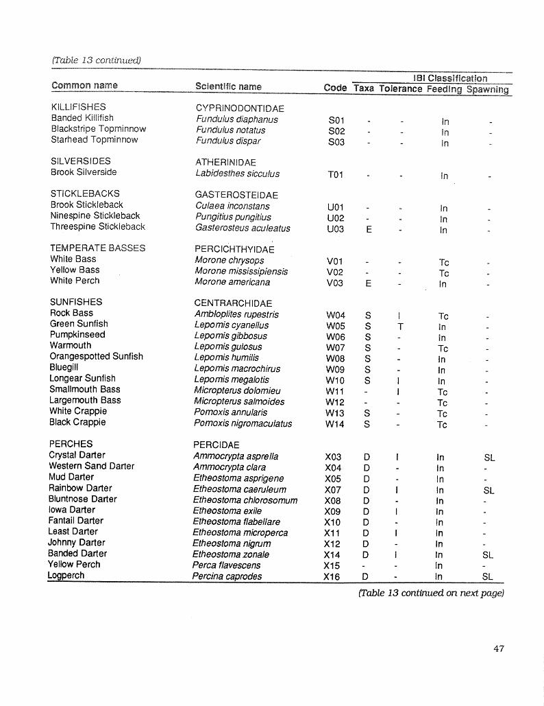
(Table 13 coT_t_ued)IBmCJassification

Common name Scientific name Code Taxa Tolerance Feeding Spawning

KILLIFISHES CYPRINODONTIDAEBanded Kiliifish Fundulus diaphanus S01 - - in -Blackstripe Topminnow Fundulus notatus S02 - - In -Starhead Topminnow Fundulus dispar S03 - - In -

SILVERSIDES ATHERINIDAEBrook Silverside Labidesthes sicculus T01 - - In

STICKLEBACKS GASTEROSTEIDAEBrook Stickleback Culaea inconstans U01 - - InNinespine Stickleback Pungitius pungitius U02 - - InThreespine Stickleback Gasterosteus aculeatus U03 E - In

TEMPERATE BASSES PERCICHTHYIDAEWhite Bass Morone chrysops V01 - - TcYellow Bass Morone mississipiensis V02 - - TcWhite Perch Morone americana V03 E - In

SUNFISHES CENTRARCHIDAERock Bass Ambloplites rupestris W04 S I TcGreen Sunfish Lepomis cyanellus W05 S T in -Pumpkinseed Lepomis gibbosus W06 S - In -Warmouth Lepomis gulosus W07 S - TcOrangespotted Sunfish Lepomis humilis W08 S - inBluegill Lepomis macrochirus W09 S - InLongearSunfish Lepomis megalotis W10 S i In -Smallmouth Bass Micropterus dolomieu W11 - i Tc -Largemouth Bass Micropterus salmoides W12 - - Tc -White Crappie Pomoxis annularis W13 S - TcBlack Crappie Pomoxis nigromaculatus W14 S - Tc -

PERCHES PERCIDAECrystal Darter Ammocrypta asprella X03 D I in SLWestern Sand Darter Ammocrypta clara X04 D - In -Mud Darter Etheostoma asprigene X05 D - In -Rainbow Darter Etheostoma caeruleum X07 D I In SLBluntnose Darter Etheostoma chlorosomum X08 D - In -Iowa Darter Etheostoma exile X09 D I In -Fantail Darter Etheostoma flabellare X10 D - In -Least Darter Etheostoma microperca X11 D I In -Johnny Darter Etheostoma nigrum X12 D - In -

Etheostoma zonale X1, D i In SLBanded DarterYellow Perch Perca flavescens X15 - - In -Logperch Percina caprodes Xl 6 D - In SL

(Table 13 continued on next page)

i

(Table I3 continued)IB_Ciassiflcation

Common name Scientific name Code Taxa Tolerance Feeding Spawning

Gilt Darte,_ Percinaevides X17 D _ In SLBlackside Darter Percinamaculata X18 D - Jn SLSienderhead Darter Percinaphoxocephala X19 D 1 in SLRiver Darter Percinashumardi X20 D - _n SLSauger Stizostedion canadense X21 - - Tc SLWalleye Stizostedion vitreum X22 Tc SLRuffe Gymnoc_phaluscemuus X26 E - In -

DRUMS SCIAENIDAEFreshwater Drum Aplodinotus grunniens Y01 - tn -

SCULPINS COTTIDAEMottled Sculpin Cottusbairdi Z01 - I In -Slimy Sculpin Cottuscognatus Z02 i In -Spoonhead Sculpin Cottusricei Z03 ] In -Deepwater Sculpin Myoxocephalus thompsoni Z04 l an -

48

........................'1/N_m_m=_=_3 .........._.......................IIr[I lll I II III II ii _ =_