IS SKILL DISPERSION A SOURCE OF PRODUCTIVITYAND EXPORTING IN DEVELOPING COUNTRIES?

John Morrow†University of Wisconsin-Madison

May 13, 2010

ABSTRACT. Recent literature claims that skill mix within firms, in contrast to average human capital,influences the entire economy. This paper provides theoretical and empirical evidence of the linkagefrom skill mix to output, inequality, productivity and exports. I develop a multisector model offirms who employ teams of workers in production. First, I consider what impact changes in theskill distribution from migration, education or outsourcing have on output. I find an increase inindustry specific workers boosts output, but in contrast to classical models, worker spillovers to otherindustries may attenuate output. Increases in diversity increase productivity and decrease inequality.Second, I consider the impact of price changes as caused by tariff reductions or subsidies. I show arise in output prices raises the total wages of a worker team, but changes relative wages withinthe team. This is because wages depend on the relative supply of high and low skill team members.Inequality will increase if the supply of high skilled workers is tight. This possibility of a sector boomcoincident with higher inequality provides a new explanation of inequality trends beyond skill biasedtechnical change. Empirically, my model motivates a novel specification that characterizes industriesas “intensive in skill diversity” or “intensive in skill similarity.” Productivity differences explainedby skill mix intensity are comparable to the magnitude of training and imported inputs combined.I also find skill mix differences explain intrasector export variation better than physical or humancapital.

JEL Codes: F11, F16, D51, J31

Keywords: wage inequality, worker teams, productivity estimation, comparative advantage

Acknowledgments. This paper has benefited from helpful discussions with Brad Barham, ChiaraBinelli, Michael Carter, Jean-Paul Chavas, Ian Coxhead, Swati Dhingra, Rob Feenstra, RebeccaLessem, Yue Li, Jim Lin, Annemie Maertens, Hiroaki Miyamoto, Shuichiro Nishioka, Yuya Taka-hashi, Scott Taylor, Carolina Villegas-Sanchez, Greg Wright, Shintaro Yamaguchi, Mian Zhu, aswell as participants at UW-Madison, OSU, and UC-Davis seminars, SOEGW 2008, MIEDC andthe CEA meetings. The usual disclaimer applies. Appendix available upon request.

† Department of Agricultural and Applied Economics, morrow1@wisc.edu.1

1. INTRODUCTION

This paper revisits the theory of the firm to incorporate the role of worker teams in production.

The mix of skills employed within a firm may range from one extreme of skill similarity to an-

other extreme of skill diversity. By skill similarity I refer to production processes which benefit

when worker teams are composed of similarly skilled workers. An example is a production line

where jobs have been broken down into equally difficult tasks, as typified by the O-Ring produc-

tion process of Kremer (1993). By skill diversity I refer to superstar production processes which

depend on the most skilled member of a team. An example is hierarchical production structures

where success is heavily tied to the quality of individuals at the top, an idea which goes back to

Rosen’s Economics of Superstars Rosen (1981). Such a fundamental distinction between methods

of production has important implications for growth, labor markets with imperfect information,

theories of the firm, wage inequality and trade.1 This paper contributes new theoretical implica-

tions by considering the role of worker scarcity when firms form teams. In addition, this paper

supports the theoretical literature by providing an empirical linkage from skill mix to productivity

within and across industries.

Theoretically I build on Grossman and Maggi (2000) who consider worker teams employed in

either skill similar or skill diverse production. Each firm hires from a population of skill levels

to form worker teams and produce goods. I extend their model to multiple sectors and arbitrary

skill distributions to exhibit new, rich forms of the Rybczynski and Stolper-Samuelson theorems.

The Rybczynski Theorem under skill diversity predicts an increase in the mass of industry specific

workers increases industry output. However, spillovers of workers into other sectors may attenu-

ate this increase in output. The Stolper-Samuelson theorem under skill diversity shows that a rise

in output prices raises the total wages of worker teams but changes relative wages within the team.

Furthermore, an increase in industry output price may decrease the wages of some workers in the

industry due to changes in the division of surplus. This possibility of growth concurrent with

decreasing wages provides a new channel for inequality beyond skill biased technical change.

1In connection to growth, Das (2005) considers research and development as a submodular process while consump-tion goods are produced using a supermodular process. In labor, Jones (2009) builds on the idea of complementaryproduction processes and intermediate goods linking sectors while Delacroix (2003) links unemployment and wagedispersion. See also Acemoglu (1999), Grossman (2004) and Moro and Norman (2005). Organizational theories of thefirm include Hong and Page (2001) who theoretically explore role of diversity in production in a novel way, suggest asearch for additional empirical evidence of richer organizational theories.

2

The primary empirical focus of this paper is establishing that skill mix, in contrast to the av-

erage level of skill, is an important determinant of productivity. There is a paucity of systematic

evidence for the role of skill similarity and skill diversity at the firm level, although some evi-

dence is suggestive.2 The theoretical model motivates an empirical specification that characterizes

industries as “intensive in skill diversity” or “intensive in skill similarity.” I use the production

structure of the model to arrive at estimable primitives of a skill diverse, multisector economy.

The approach is to specify production in a neoclassical form where skill mix enters as labor aug-

menting technology. The labor augmenting technology may be “similar skill loving”, “diverse

skill loving” or neutral for each industry. The specification is estimated for a cross section of firms

in over thirty developing countries using the Enterprise Surveys collected by the World Bank. In

developing countries productivity differences due to skill mix should be pronounced due to both

greater heterogeneity in educational attainment and labor abundant production.

I find that over two-thirds of developing country firms belong to sectors which are significantly

characterized as either “similar skill loving” or “diverse skill loving.” The estimates provide a

ranking of intensity across industries from skill similar to skill diverse. This parallels the concept

of factor intensity in classical trade theory. As the model predicts linkages from such intensities

to inequality, the magnitudes of the estimates are particularly relevant in a developing country

context.3 Within industries, I rank firms by the level of productivity explained by skill mix. Using

this ranking, I find the difference between the 75th and 25th percentiles are 9-13%, comparable to

the effects of training and imported inputs combined.

The second empirical focus of this paper is testing the linkage from skill mix to comparative ad-

vantage at the firm level.4 Recent theoretical work has shown that skill mix may predict patterns

2Andersson et al. (2009) find that firms with high potential payoffs for selecting the right products (a task assistedby worker talent) pay higher starting salaries and select superstars who have a history of success. Martins (2008)also uses matched employer-employee data to tackle competing theories of the relationship between wage dispersionon firm performance, finding a positive relationship which becomes negative once firm and worker fixed effects areconsidered.3The relationship between trade and inequality has generated a vast literature. For surveys, see Kremer and Maskin(2003), Winters et al. (2004) and Goldberg and Pavcnik (2007).4Again evidence is sparse or suggestive. Mamoon and Murshed (2008) find developing countries with a high level ofschooling experience smaller increases in wage inequality following trade. This is consistent with the idea that highskill countries have a comparative advantage in complementary production relative to low skill countries which bestutilize scarce high skill workers in diverse production.

3

of trade and expected wage shifts resulting from trade.5 My approach to testing trade implications

joins two strains of the trade literature. The first literature emphasizes the role of heterogeneous

firm level productivity as a selection mechanism for exports in the presence of trade frictions (e.g.

Melitz (2003)). The second literature explains productivity differences as outcomes of heteroge-

neous worker matches to jobs.6 If productivity differences arise from a relatively high endowment

of diverse or similar labor, the predicted pattern of trade depends on moments of the skill dis-

tribution beyond the mean. I use a non-linear function of skill mix to explain firm productivity

and account for firm exports, revealing a new connection from skill similarity and skill diversity

to trade. Productivity differences explained by skill mix predict intrasector exports better than

physical or human capital.

The rest of this paper is organized in six sections. Section 2 lays out the model setting while

Section 3 develops implications in the form of new Rybczynski and Stolper-Samuelson theorems.

Section 4 puts forth the production specification and estimates the relative importance of skill mix

within industries. Section 5 estimates the relationship between propensity to export and skill mix.

Section 6 concludes.

2. A SKILL DIVERSE MULTI-SECTOR ECONOMY

This section begins with the model setting where firms form production teams from a hetero-

geneous pool of workers. After defining a perfectly competitive equilibrium, I consider the allo-

cation of workers within and across firms. Finally, I construct the wage schedule which supports

the efficient equilibrium. General equilibrium implications are pursued in the following section.

2.1. Model Setting. Consider an economy populated with a mass L of workers of varying skill

levels q. Denote the distribution of skills within the population by Φ(q), and assume that Φ has

a continuous pdf with full support on [0, ∞) and finite mean.7 Equilibrium wages received by a

5Ohnsorge and Trefler (2007) construct a model in which a high correlation between worker attributes amounts to arelative abundance of one of the factors, resulting in a pattern of trade based on a second moment of the skill distribu-tion. In Bougheas and Riezman (2007) both first order stochastic dominance and mean preserving spreads which alterthe skill distribution predict a pattern of trade.6From a comparative advantage perspective, both Manasse and Turrini (2001) and Yeaple (2005) result in the selectionof high skill inputs into export activities. Both papers are competing explanations for the stylized facts of a growingskill premium and productivity differences between exporters and non-exporters. Costinot and Vogel (2009) considera continuum of workers and goods produced with different skill intensities and considers the implications of skill andtechnology shifts in autarky, North-South and North-North trade. In contrast, I investigate a different channel basedon the skill mix of worker teams rather than the skill of individual workers.7I show in the appendix that the value of production in the economy is bounded if and only if Φ has a finite mean sothis assumption entails no loss of generality.

4

worker of skill level q are written as w(q). Workers supply labor inelastically, and choose employ-

ment at the highest wage available in one of N + 1 sectors Si, i ∈ {0, . . . , N}. This results in an

optimal sorting problem of workers within firms and across sectors.

Each sector i produces a single type of good, whereas goods within a sector i are indistinguish-

able. Workers incomes consist of their wages w(q) and have identical homothetic preferences

U(y0, . . . , yN) over bundles of outputs y ≡ (y0, . . . , yN). Output prices are denoted {pi}Ni=0. For

the moment I take prices {pi}Ni=0 as exogeneous, consistent with the assumption of a small open

economy, in order to focus on the production side.

A firm within sector i has a production technology Fi which produces goods by pairing workers

with skill levels q and q′, producing a quantity Fi(q, q′). Each production technology Fi is symmet-

ric, homogeneous of degree one and twice continuously differentiable. All firms maximize profits.

Firms face perfectly competitive output prices pi and input prices w(q). Thus each firm takes pi

and w(q) as set by the market and chooses to pair workers of skills q, q′ in order to maximize

profits πi(q, q′) where

πi(q, q′) ≡ piFi(q, q′)− w(q)− w(q′)(2.1)

I now formalize the idea that different industries might better use different mixes of skill within

their workforce. This is done by adding structure to the production technologies, which will

result in a ranking of the skill diversity content across sectors. S0 is a complementary sector where

the production technology F0 supermodular in skill inputs. In this case, supermodularity of F0 is

equivalent to F012(q, q′) ≥ 0 so worker skills are complementary. Grossman and Maggi (2000) show

that the revenue maximizing skill pairing within such a supermodular sector is to pair workers of

identical skills and this pairing also occurs in the equilibrium of this model. It is only necessary to

consider a single supermodular sector S0 as investigation shows one such complementary sector

dominates the others and crowds them out in equilibrium.

For each sector Si, with i > 0 the production technology Fi(q, q′) is submodular. Submodularity

of Fi is equivalent to Fi12(q, q′) ≤ 0 so workers skills are imperfect substitutes for each other.8 This

8Note the often used Cobb-Douglas form for skill inputs cannot distinguish skill inputs as being supermodular orsubmodular since the cross partials are always positive (if output is homogeneous and increasing in inputs), implyinga supermodular form. For instance, Ohnsorge and Trefler (2007) model heterogeneous workers with “human capital”and “brawn” attributes which enter production in a Cobb-Douglas fashion, implying complementarity between theattributes across all sectors. See Kremer and Maskin (1996) for a discussion of the necessity of imperfect substitutabilityof skills in explaining worker inequality and segregation.

5

implies production becomes mostly dependent on the highest skill worker of the team. Holding

total skills q + q′ constant, firm revenues in these sectors increase as the skill levels of employed

workers diverge. However, the allocation of labor across many sectors creates a conflict: which

sectors will get the most diverse workers and how will they be paired? I show that the most

important difference between sectors is their input intensities, akin to other models based on factor

intensity.9 Intuitively, the “most submodular” sector can best utilize a diverse workforce and

should therefore be allocated the most diverse workers. This intuition bears out in equilibrium,

provided the production technologies satisfy the following diversity ranking � between sectors.

Definition (Diversity Ranking). Si is more diverse than Sj, written Si � Sj, if and only if piFi(1, x)/pjFj(1, x)is strictly increasing for x ≥ 1.

If for each pair of sectors Si and Sj either Si � Sj or Si � Sj then � is a complete diversity ranking.

Intuitively, Si � Sj says that the relative output of Si over Sj increases as more diverse workers

are employed. In order to make this ranking concrete, consider the ranking in the context of CES

production functions. In this case it is straightforward to show that the elasticity of substitution

measures the capacity of a technology to efficiently use diverse labor. The diversity ranking in-

duced is given in the following Lemma.

Lemma (CES Ranking). Suppose each Fi is CES, specifically Fi(q, q′) ≡ Ai(qρi + q′ρi)1/ρi . Then Si � Sjif and only if ρi > ρj so CES production technologies imply a complete diversity ranking.

Proof. See Appendix. �

The supermodularity of F0 guarantees that Si � S0 for all i > 0. This makes sense as the

productivity of a submodular technology Fi increases in diversity, while the productivity of F0 is

maximized when identical workers are employed. It is also clear that � is transitive, i.e. Si � Sj

and Sj � Sk implies Si � Sk, so� provides a natural way to rank all of the sectors Si. Consequently,

I hereafter maintain Assumption 1.10

Assumption 1. The diversity ranking � is complete and SN � SN−1 � . . . � S1 � S0.

I consider competitive equilibria in which all firms maximize profits and economy wide revenue

is maximized. To account for the sorting of workers, define two assignment maps M(q) = q′ and

9Of course, if some sectors strictly dominate others, for example through a superior Hicks neutral technology or highprice, such dominant sectors will soak up all the workers. Consequently the most interesting sectors are those whichemploy workers in equilibrium and therefore consideration is restricted to producing sectors.10A more empirically motivated criterion which implies completeness (and is almost equivalent) is to define the“elasticity of diversity” for each sector i by Ei ≡ ∂ ln Fi(1, x)/∂x. Then there is a complete ranking of sectorsSN � SN−1 � . . . � S1 � S0 so long as EN ≥ EN−1 ≥ . . . ≥ E0.

6

ι(q) = i. M(q) pairs a worker of skill q to a worker of skill q′ while ι(q) assigns the paired workers

(q, M(q)) to sector i. A competitive equilibrium therefore consists of assignments M(q), ι(q) and

wages w(q) which satisfy the following conditions:

Definition. An efficient, competitive equilibrium is a wage schedule w(q), team compositions(q, M(q)), and sector assignments ι(q) which satisfy:

(1) (Profit Maximization) Each triple (q, M(q), ι(q)) is consistent with profit maximization:

πι(q)(q, M(q)) ≥ πi(q, q′) ∀i, q′

(2) (Perfect Competition) Each triple (q, M(q), ι(q)) yields zero profits, πι(q)(q, M(q)) = 0.(3) (Efficiency) Economy wide revenue is maximized.

Conditions (1) and (2) together guarantee a “no arbitrage” condition for workers. They guar-

antee that breaking up an equilibrium pair of workers (q, M(q)) and reassigning them to different

sectors or teams can only yield weakly negative profits. Under conditions (1) and (2) workers can-

not be lured away from equilibrium through arbitrage. Condition (3) is an equilibrium selection

constraint that restricts attention to first best equilibria.

I now provide implications for the allocation of workers to each other through teams (q, M(q))

and across sectors through ι(q). Shortly these allocations will be supported by wages so that the

allocative results discussed here are the equilibrium skill allocation, fixing production and endoge-

nous sorting in the economy.

2.2. Allocation of Skill Diversity by Sector. I now derive the allocation of workers to teams

and sectors. This allocation hinges heavily on the concept of skill dispersion. While there are

potentially many ways to measure skill dispersion within a firm, this paper uses the following

idea. For an equilibrium matching function M(q), suppose firm i employs workers with skill

levels (qi, M(qi)) and firm j employs the team (qj, M(qj)), where by convention qi ≤ M(qi) and

qj ≤ M(qj). Then a natural definition is that firm i employs more diverse labor than firm j if

M(qi)/qi ≥ M(qj)/qj. If this holds when comparing every firm i in sector Si with every firm j in

sector Sj, then sector Si employs more diverse labor than sector Sj. Assumption 1 guarantees that

entire sectors can be ranked by skill diversity using the ranking �.

Proposition. Under Assumption 1, any equilibrium allocation exhibits skill ratios {t̂i}, increasing in i,where if (q, M(q)) are assigned to Si then M(q)/q ∈

[t̂i, t̂i+1

). The ratios are fixed for i > 1 by

piFi(1, t̂i) = pi−1Fi−1(1, t̂i)

Proof. See Appendix. �7

Figure 2.1(a) illustrates this Proposition for a hypothetical M(q). For a team (q, M(q)), the x-axis

tracks the skill level of the low skill worker q and the y-axis plots the skill level of his partner M(q).

As the Figure shows, teams where the skill ratio M(q)/q is the highest (close to q = 0) must work

in the most diverse sector, S5. If the skill ratio within a team decreases slightly, profit maximizing

firms will employ the team in the next most diverse sector, S4 and so on. In conclusion, skill

intensity ratios play a similar role as factor intensities in the multi-sector Heckscher-Ohlin model,

except that in Heckscher-Ohlin there is a unique intensity in each sector whereas here there is a

range of skill ratios.

FIGURE 2.1. Skill Ratio Cutoffs by Sector

(A) Skill Ratio Cutoffs by Sector (B) Sector Assignments fixed by M(q)

So far, Proposition 2.2 has pinned down ι(q) (the equilibrium sector of a worker of skill q), given

M(q). This follows because when M(q) is known, M(q)/q is known and consequently the skill

ratio cutoffs {t̂i} imply the sectoral assignment (2.2).

ι(q) =

N, M(q)/q ∈ [t̂N , ∞)...

...

1, M(q)/q ∈ [t̂1, t̂2)

0, M(q)/q ∈ [1, t̂1)

(2.2)

I now discuss how M(q) is determined in order to fix the equilibrium allocation (q, M(q), ι(q)).

Getting from the assignment (2.2) to the matching function M(q) proceeds in three steps:

(1) Aggregate the sectors {Si}i≥1 into a single submodular sector using Assumption 1.8

(2) Show in the S0 sector workers pair assortatively, i.e. M(q) = q. In the sectors {Si}i≥1

workers pair according to maximal cross matching.

(3) Show efficiency requires the skill set of workers assigned to the S0 sector is of the form [t, t].

With (2), this fixes (q, M(q)) for the sectors {Si}i≥1. Proposition 2.2 then assigns workers

among the N sectors since M(q) is known.

As these steps are somewhat involved, they are left to the appendix. Here I focus on the resulting

form of the matching function M(q). Within the S0 sector, workers are paired with identical skills.

As the diversity loving sectors {Si}i>0 best utilize pairs of low and high skill workers, it is sensible

that the skill range of workers employed in S0 is the range (t0, t0) with

t0 ≤ median skill level of population ≤ t0

So the “middle of the road” workers are employed in S0. I now detail an intuitive argument for

fixing the cutoffs (t0, t0). The revenue generated per unit of skill in the S0 sector must be at least

as high as in any other sector. This results in skill cutoffs (t0, t0) as fixed in Equation (2.3):

p0F0(1, 1)/2︸ ︷︷ ︸Revenue per unit of skill in S0

= p1F1(t0, t0)/(t0 + t0)︸ ︷︷ ︸Revenue per unit of skill in least submodular sector

(2.3)

The remaining workers are employed in pairs (q, mS(q)), where mS(q) is the maximal cross

matching of workers unassigned to S0. The function mS(q) pairs the highest and lowest skilled

workers first, the second highest skilled with the second lowest skilled, and so forth. Formally,

letting ΦS(t) ≡∫ t

0 1[0,t]∪[t,∞)dΦ be the distribution of workers employed in the sectors {Si}i>0,

the maximal cross matching mS(q) must satisfy ΦS(q) + ΦS(mS(q)) = 1. Therefore mS(q) can

be written mS(q) = (ΦS)−1(1−ΦS(q)). The final allocation is therefore given by Equation (2.4),

where the skill cutoffs ti, ti are fixed by (t0, t0) and Equation (2.2).

M(q) ≡

mS(q), q ≤ t0

q, q ∈ (t0, t0)

mS(q), q ≥ t0

ι(q) =

N, q ∈ (0, tN−1]...

...

0, q ∈ (t0, t0)...

...

N, q ∈ [tN , ∞)

(2.4)

9

Although the geometry of Equation (2.4) is simple, as illustrated in Figure 2.1(b). Once the worker

match function M(q) is fixed by Equation (2.4), Proposition 2.2 then pins down ι(q) as in Figure

2.1(a). This induces the skill cutoff ranges for each sector Si of low skill workers q ∈ (ti, ti−1] paired

with high skill workers M(q) ∈ [M(ti−1), M(ti)). These allocations are next supported by wages.

2.3. Wages Under Multisector Diversity. Up until now, I have only derived necessary conditions

for a competitive equilibrium, which fix a unique assignment of workers to firms. I now construct

wages across sectors which support this assignment so that the allocation of workers described

above is a competitive equilibrium. The assumption of multiple sectors will yield differing skill

premiums across sectors for both low and high skill workers. This highlights a principle of worker

symbiosis and parasitism: the division of surplus between high and low skill workers depends on

the joint skills of the workers, as well as aggregate labor market conditions.

For brevity I only consider wages w(q) which are continuous and differentiable in the interior

of each sector. Since there is a continuum of firms, competitive behavior must drive profits to zero.

In the complementary S0 sector where q ∈ (t0, t0), workers are paired with identical skills so the

zero profit condition implies that

w(q) + w(q) = p0F0(q, q) = p0F0(1, 1) · q

So for q ∈ (t0, t0), w(q) = w0q where w0 ≡ (p0/2) · F0(1, 1). However, wages in the sectors {Si}i≥1

are more interesting. This is because a firm in {Si}i≥1 must lure both high and low skill workers

away from S0 by offering wages above w0q, and I term the additional wages required a diversity

premium. Notice that the diversity premium is different from a skill premium: both low and high

skill workers receive a diversity premium in addition to w0q which increases in skill.

Next I construct wages recursively starting with sector S1 and proceeding to S2, S3, and so on.

Workers in S1 have skills q ∈ (t1, t0]∪ [M(t0), M(t1)) and once wages are found for q ∈ (t1, t0], the

zero profit condition fixes wages for q ∈ [M(t0), M(t1)). First, a worker with skill t0 employed at

the cusp between S0 and S1 must be employable in either sector, so w(t0) = w0t0 since w0 is the

wage rate paid per unit of skill in the S0 sector. Second, for any wages w the first order necessary

conditions for profit maximization by firms must hold. The profit maximization conditions are10

Equations (2.5) for i ≥ 1.11

piFi1(q, M(q)) = w′(q) and piFi

2(q, M(q)) = w′(M(q))(2.5)

Thus, for q ∈ (t1, t0], equilibrium requires that w′(q) = p1F11 (q, M(q)) and integrating from t0

down to q < t0 gives

w(q) = w(t0)−∫ t0

qp1F1

1 (s, M(s))ds, q ∈ (t1, t0]

Proceeding inductively, the recursive relationship for wages across sectors at skill levels below the

median are given by

w(q) =

w0q, q ∈ (t0, t0)

w(t0) −∫ t0

q p1F11 (s, M(s))ds, q ∈ (t1, t0]

w(t1) −∫ t1

q p2F21 (s, M(s))ds, q ∈ (t2, t1]

......

w(tN−1) −∫ tN−1

q pN FN1 (s, M(s))ds, q ∈ (0, tN−1]

(2.6)

Equation (2.6) highlights the fact that the wage an individual receives depends not only on his

raw skill but also the wages of those in less diverse sectors. Consider a worker who is the lower

skill member of a team in sector Si, i ≥ 0. His wage is a sector specific wage w(ti−1) plus an

integral related to the curvature of Fi. Since w(ti−1) is tied to wages in sector Si−1, wages in sector

Si are recursively “pegged” to wages in Si−1 and so on up to S0.

Equilibrium wage pegs are better understood by decomposing wages into variable and sector

level components. First, define the shadow wage a worker would receive in an economy which

has access to a single technology Fi, which I label wShadowi (q). From Equation (2.6), shadow

wages for the diversity loving sectors Si are fixed by

wShadowi (q) ≡ piFi(qmed, qmed)/2−

∫ qmedq

piFi1(s, M(s))ds

11Other approaches to obtaining wages for heterogeneous workers in the absence of firm competition include bargain-ing between workers (e.g. Delacroix, 2003) and the N-worker coalitional model of (Sherstyuk, 1998).

11

where qmed is the median of the skill distribution. Then wages (Equation 2.6) can be written

recursively as

w(q) =

w0q, q ∈ (t0, t0)

wShadowi (q)︸ ︷︷ ︸Variable

Component

+ wi(ti−1)− wShadowi (ti−1)︸ ︷︷ ︸

Sector-wide

Component

, q ∈ (ti, ti−1](2.7)

Equation (2.7) shows that wages are composed of a variable shadow wage and a sector-wide

component. The shadow wage is fixed by the technology of Si in isolation of other technologies.

The sector-wide component is fixed by the allocation of skill across all sectors which determines

the cutoffs ti−1.

Although “pegged”, wages given by Equation (2.7) have the usual properties. For instance,

they are strictly increasing in skill. Wages are also bounded below by the S0 shadow wages of

w0q since the sectors {Si}i≥1 must lure away workers from S0. Wages are also convex in skill

for the following economic reason: wages are fixed by the profit maximization Equations (2.5).

Through duality wages are also fixed by cost minimization in skill choice, implying some variety

of convexity. The specific property is that w′(q) is (essentially) increasing.12 These properties of

the wage structure are summarized in this Proposition:

Proposition. The wage schedule w(q) has the following properties:(1) w(q) is strictly increasing and convex.(2) w(q) is bounded below by the S0 shadow wages w0q.(3) w′(q) is increasing where defined, and elsewhere limq→x− w′(q) ≤ limq→x+ w′(q).

Proof. See Appendix. �

The wage schedule of Equation (2.6) supports a competitive equilibrium. In order to show this,

it is sufficient to guarantee that if a firm deviates from a skill pairing (q, M(q)), then the firm

obtains non-positive profits. The basic argument relies on checking the first order conditions of

any firm who deviates from equilibrium. Leaving details to the appendix, the fact that wages

support the proposed equilibrium is stated in the following Proposition:

Proposition. Wages given by Equation (2.6) support an efficient competitive equilibrium.

12At the cusp levels of skill {ti} and {M(ti)}, w′(q) is not defined but essentially increases discontinuously as the cuspfrom lower to higher skill is crossed. Technically, the one sided derivatives of w(q) are defined at the cusps {ti} and{M(ti)} and the left hand limit is less than the right hand limit.

12

Proof. See Appendix. �

This section has detailed the allocation of workers to both teams and sectors in any efficient,

competitive equilibrium. The next section proceeds to consider the effects of price and endowment

changes in general equilibrium, deriving variations of the Rybczynski and Stolper-Samuelson the-

orems.

3. GENERAL EQUILIBRIUM IMPLICATIONS

This section extends canonical results of the trade literature, the Rybczynski and Stolper-Samuelson

theorems. The Rybczynski theorem predicts how production changes in response to a change

in endowments. In this model setting, the most interesting changes in the skill distribution are

those which in some way change the diversity of skills in the workforce. Here I provide a defi-

nition of such “changes in diversity” and show that increases in availability of a sector’s inputs

increase the mass of workers employed in the sector. Associated with the Rybczynski theorem is

the “magnification effect”, which means that an increase in sector endowments results in a more

than proportional increase in output. In this section, I show that the addition of new workers

causes magnification through more efficient worker sorting. However, this effect disappears if

changes in the skill distribution cause appreciable spillovers of workers across sectors.

I then present two variations on the Stolper-Samuelson theorem. The first shows an increase

in output price increases total factor returns in a sector, namely total wages per worker pair. This

increase in wages is independent of endowments, in the spirit of the Stolper-Samuelson theorem

(e.g. the review in Lloyd, 2000). Unlike the Stolper-Samuelson theorem, an increase in output

price also reallocates workers to the more profitable sector.13 In contrast, the second variation

of the Stolper-Samuelson theorem shows that surplus sharing within teams changes in response

to price changes. Low skill workers will get a larger wage share if high skill workers are abun-

dant, whereas high skill workers benefit if their skills are rare. Thus the wages of either member

of a worker team may decrease once a sector booms, providing a new channel from growth to

inequality.

3.1. Rybczynski Under Skill Diversity. Characterizing precisely what diversity means for a given

distribution of skills Φ is a difficult task. This is because without additional structure on Φ it is

13Upward sloping supply of labor in each sector is an important feature missing from classical trade theory, as discussedby Ohnsorge and Trefler (2007).

13

hard to predict equilibrium changes, or come to terms about the meaning of a particular change.

I settle on a “results based” definition which allows for a Rybczynski type prediction. To sim-

plify the exposition I first consider only two sectors S0 (which pairs identical workers) and S1

(which pairs diverse workers). Having seen the mechanics of the two sector case, the multisector

Rybczynski theorem is presented.

Define a change in a skill endowment Φ to a new skill endowment Φ̃ a skill shock and normalize

the mass of labor to one for both distributions. I define three types of skill shifts from Φ to Φ̃: Low

Skill Shocks, High Skill Shocks and Diverse Skill Shocks.

Definition (Skill Shocks). Let Φ and Φ̃ be two skill distributions and (t0, t0) the range of workerskills employed in S0 under Φ.

(1) (Low Skill Shock) Φ(t0) ≤ Φ̃(t0) and Φ̃(M(t0)) = Φ(M(t0)).(2) (High Skill Shock) Φ(t0) = Φ̃(t0) and Φ̃(M(t0)) ≤ Φ(M(t0)).(3) (Diverse Skill Shock) Φ(t0) ≤ Φ̃(t0) and Φ̃(M(t0)) ≤ Φ(M(t0)).

In the case of a Low Skill Shock, the pool of workers in the low skill range of S1, q ∈ (0, t0],

expands. This provides more matching opportunities for diverse teams, causing S1 to draw in high

skill workers at the expense of S0. Therefore the mass of workers employed in S1 increases, while

the range of skills in S0 decreases in level. High Skill Shocks are similar. Finally, a Diverse Skill

Shock is the simultaneous combination of a Low Skill Shock and High Skill Shock and therefore

increases the mass of workers employed in S1. If the diverse skill shock consists of adding an equal

mass of low and high skill workers, workers resort, but on net the skill range of S0 is unaffected

because the resorting will all occur in S1. Each of these allocational effects carry through to the

multisector case which I now discuss.

The effect of new workers with more than two sectors is shown in Figure 3.1. Figure 3.1(a)

displays the allocation of workers across sectors before a skill shock, while Figure 3.1(b) displays

the reallocation after the endowment of high skill workers in S4 increases. Figure 3.1(c) shows that

adding high skill workers to the economy shifts up the matching function M(q). This is because

low skill workers can be matched with new, higher skill team members, increasing the ratio of

skills per team. Once M(q) shifts up, it determines new skill ranges for each sector. As shown, the

range of low skill workers [t4, t3] employed in S4 increases by shifting t3. The range of high skill

workers [M(t3), M(t4)] expands as well, maintaining skill diversity in S4. While new low skill

workers join S4, some high skill S4 workers will spill over into S3.14

FIGURE 3.1. Skill Endowments and Sectoral Allocation

(A) Sector Assignments fixed by M(q)

(B) Re-matching from a High Skill Shock

By keeping track of how workers are employed as in Figure 3.1, I arrive at a new version of

the Rybczynski Theorem. Consider an economy with an initial skill endowment Φ and a mass of

workers L, to which is added a distribution of workers Ψ with mass P. This added endowment

of workers might be migrants, newly trained workers, or the result of outsourcing. To mirror the

concept of a Diverse Skill Shock, further assume Ψ is composed of workers with the right skill

levels for one sector Si. Formally, Ψ has support on some set [ti, ti−1] ∪ [M(ti−1), M(ti)]. Once

Ψ is pooled with the initial endowment Φ, the supply of workers to Si has increased. The new

equilibrium allocation will result in more workers employed in Si, but more precisely, the total

output in the sector will increase. This result is summarized in Proposition 1.

A stronger form of the Rybczynski theorem is the “magnification effect,” meaning that an

increase in sector specific endowments results in a more than proportional increase in output.15

As seen above, the addition of workers to the economy causes spillovers of workers across sec-

tors. Such spillovers preclude any unconditional magnification effect because added endowments

can contain a high percentage of workers who will spillover into other sectors.14 Thus worker

spillovers may attenuate or strengthen output increases in the sector, altering magnification ef-

fects.

However, if the worker spillover effect is purged, new and more efficient resorting of workers

will lead to magnification. To see this, suppose the skill endowment increases by adding a skill

distribution Ψ. To purge the worker spillover effect outside of Si, assume again that Ψ has sup-

port on [ti, ti−1] ∪ [MΦ(ti−1), MΦ(ti)], and additionally assume equal masses of low and high skill

workers. Then no worker spillovers occur, but the new allocation of workers in Si is optimal and

therefore output is higher than if Φ and Ψ are allocated to Si separately. I summarize these results

regarding magnification in Proposition 1.

Proposition 1. Increases in sector specific skills increase sector output. Absent spillovers, output is mag-nified due to more efficient worker sorting.

Proof. See Appendix. �

These results are in sharp contrast to model settings which ignore the team aspect of produc-

tion. From the team based perspective, migration and education policies designed to support

particular industries or growth should consider the relative scarcity of differently skilled workers.

Policies targeting groups of fairly homogeneous skills (refugees, the uneducated, specialist work-

ers) should keep in mind the availability of their potential co-workers as this may influence their

final industry of employment.

Finally, consider the effect of adding more diverse workers to Si. Again suppose Ψ has support

on [ti, ti−1] ∪ [MΦ(ti−1), MΦ(ti)] with equal masses of low and high skill workers. Denote the

respective worker matching functions as MΦ and MΨ, making the dependence of matches on the

skill distribution explicit. In the case that MΨ(q) ≥ MΦ(q) for all q, Ψ generates more diverse

teams than Φ (i.e. MΨ(q)/q ≥ MΦ(q)/q for all q). Therefore productivity (output per unit of skill)

14For instance, suppose the skill distribution is Φ and a distribution of workers Ψ migrate to join the Φ workers. To bespecific, say the new Ψ workers have low skills in the range [ti, ti−1], those skills used by the Si sector. A Heckscher-Ohlin setting would predict a boom in the Si sector through magnification. However, in this model, the outcomedepends on the supply of high skill workers available to work with the new migrants in Si. If the host country’sdistribution Φ is thin on workers in the range [M(ti−1), M(ti)], then new migrants will force spillovers into other sectorssuccessively; first the Si−1 sector then Si−2, etc. Conversely, if the host country is abundant in the [M(ti−1), M(ti)] skillrange, then magnification effects could be large since the migrants might be very efficient additions to the sector.

16

under Ψ is uniformly greater than under Φ because of submodularity. Formally for all q:

Fi(q, MΨ(q))/ (q + MΨ(q)) ≥ Fi(q, MΦ(q))/ (q + MΦ(q))

It can be shown that once the more diverse Ψ is added to Φ, a uniform increase in productivity

still holds.

The second effect of adding more diverse workers is to increase shadow wages wShadowi (q)

for low skill workers.. To see this, recall

wShadowi (q) = piFi(qmed, qmed)/2−

∫ qmedq

piFi1(s, M(s))ds

and Fi12 ≤ 0 so if the match function increases, low skill shadow wages increase. Since there

are no worker spillovers, the sector wide component of wages is unaffected in Si. However, the

lowest skill worker ti has a higher wage which propagates to low skill workers in Sj for j > i

through wi(ti) while Fi(ti, M(ti)) is fixed. In summary, adding more diverse workers decreases

inequality in more diverse sectors. These effects of adding more diverse workers are summarized

in Proposition 2.

Proposition 2. Suppose sectoral skill diversity increases by adding equal masses of low and high skillworkers. Then

(1) Productivity increases across all teams in the sector.(2) Low skill wages rise in the sector.(3) Wage inequality decreases in sectors more diverse than the receiving sector.

In addition, the distribution of skills influences relative wages within teams when output prices

change, which I now turn to.

3.2. Stolper-Samuelson under Skill Diversity. The Stolper-Samuelson Theorem, along with mod-

ifications and extensions, has a long history (e.g. Neary, 2004). I now develop two Theorems in

the spirit of Stolper-Samuelson with surprising implications. The first is in line with the canonical

result that a rise in the world price pi of a good increases returns to the intensive factor of a sector.

In this case I consider the aggregate wages of the two workers (q, M(q)) paired in a sector relative

to all other sectors. The second version I consider concerns the wage distribution between low

and high skill workers. A rise in a sector’s good price will raise aggregate wages in the sector, but

will also change relative wages within worker teams due to the endogenous reallocation of work-

ers across sectors. I show that the indirect reallocation effect of worker sorting may dominate the17

direct “Stolper-Samuelson” effect of a rise in good price. In particular, the welfare implications of

Grossman and Maggi (2000) depend on the assumption of a symmetric skill distribution and are

overturned once empirically motivated distributions are considered.

For the first Stolper-Samuelson result, consider a rise in output prices pi in a diverse sector Si

with i ≥ 1. Increases in pi make production in Si more profitable, thereby expanding the range of

worker teams employable in the sector. This effect is depicted in Figure 3.2(a). As more worker

teams become profitable to employ the sector expands, stealing away worker teams from adjacent

sectors.15

FIGURE 3.2. Stolper Samuelson Effects

(A) Effect of Increased Output Price

Now consider the effect of output prices on wages. If the output price pi rises to p̃i, then for

any team (q, M(q)) employed in Si, revenues piFi(q, M(q)) rise. Perfect competition implies that

firm revenue equals w(q) + w(M(q)) and therefore total wages increase with output price. At the

same time, “new” teams (q, M(q)) who join Si after the price increase also receive w(q) + w(M(q))

equal to firm revenue. As revenue is maximized in equilibrium, it must be that the “new” team

receives total wages at least as high as the revenue generated in their “old” employment. Finally,

revenues remain unchanged outside of Si, so total wages paid by any firm outside of Si do not

change. Therefore total wages w(q) + w(M(q)) for incumbent and new employees in Si increase.

15Note there is only one instance in which a change in output prices can affect the composition a worker team. Thisis when the team is either created by pulling (q, M(q)) from the S0 where workers are paired with identical skills, or ateam is destroyed by moving from S1 into S0. Outside of this case, the effect of a change in pi on the range of workers[ti, ti−1] employed in Si can be quantified by defining the following skill and revenue elasticities:

Eti ,pi ≡ d ln ti/d ln pi, Eti−1,pi ≡ d ln ti−1/d ln pi, ERj ,ti≡ d ln pjFj(ti, M(ti))/d ln dti

in which case it can be shown that

Eti ,pi =[ERi+1,ti

− ERi ,ti

]−1< 0 and Eti−1,pi =

[ERi−1,ti−1

− ERi ,ti−1

]−1> 0

18

Investigation shows total real wages [w(q) + w(M(q))] /pi = Fi(q, M(q)) stay constant. These

effects of a rise in output price are recorded as Proposition 3.

Proposition 3. If output price pi increases then output and employment in Si expand. In addition:

(1) Total nominal wages for each team in Si increase, but are constant outside of Si.(2) Total real wages [w(q) + w(M(q))] /pi for each team in Si stay constant.

In contrast to models where inputs are mobile but homogeneous, Proposition 3 shows that

output price effects on total factor returns are quarantined to the affected sector. What is surprising

is that despite this quarantine on total wages for a team, individual wages outside the affected

sector change. This occurs because worker reallocation changes the division of total wages within

a team. Thus, there is a second Stolper-Samuelson effect on input prices which I now consider.

3.3. Stolper-Samuelson within Sectors. Although total wages increase following an increase in

good price, it is not necessarily true that all wages rise. In fact, the wages of a high or low skill

worker employed in a “booming” sector may fall. A rise in good price causes the sector to expand,

drawing in more workers and changing the relative scarcity of low and high skill workers in the

sector. This changes the division of wages within teams. The crucial determinant of how sector

expansion changes wages is the elasticity of matching EM,q where

EM,q ≡ d ln M(q)/d ln q = Φ′(q)/Φ′(M(q))︸ ︷︷ ︸Relative Scarcity of Skills

· (−q/M(q))(3.1)

EM,q captures the elasticity of high skill matches M(q) in response to a small change in q. It mea-

sures how quickly high skill matches M(q) decrease as q increases. As a sector expands, it draws

in worker teams at the margins of the sector, i.e. the teams (ti−1, M(ti−1)) and (ti, M(ti)). Wage

changes within teams are characterized by the elasticity of matching EM,ti−1, which I now detail.

Increases in sector output price pi will have two effects on wages: direct effects through pi

within the sector and indirect effects through ti−1 by drawing new workers into the sector. As

seen in Figure 3.2(a), the indirect effect will expand the skill range (ti, ti−1] ∪ [M(ti−1), M(ti)) of19

workers employed in Si. The two effects are decomposed in Equation (3.2).

dwi(q)/dpi = ∂wi/∂pi︸ ︷︷ ︸Direct Effect on Wages

+ ∂wi/∂ti−1 · dti−1/dpi︸ ︷︷ ︸Indirect Effect of New Workers

= −∫ ti−1

qFi

1(s, M(s))ds︸ ︷︷ ︸(−)

+w(ti−1) + w(M(ti−1))

1− EM,ti−1︸ ︷︷ ︸(+)

(3.2)

The decomposition of Equation (3.2) is striking because the direct effect of an increase in output

price is to decrease wages for low skill workers.16 Paradoxically, when revenues rise, low skill

wages fall in the absence of entry by new workers. These lost wages “trickle up” to each low skill

worker’s team member. From the perspective of the firm, the importance of high skill workers

increases with revenues since they are the essential ingredient to a diversity loving technology. For

high skill workers, the direct effect of an increase in output prices is to capture all new revenues,

and also some wages formerly paid to low skill workers.

This direct “trickle up” effect is counteracted by the indirect effect from new workers entering

the sector. This indirect effect depends on the relative supply of low and high skill workers to

the sector, as captured by the elasticity of matching in Equation (3.1). If low skill workers are

abundant, the indirect effect will be small since even a small increase in wages will draw many

low skill workers to the sector. Potential low skill entrants have skills in the range (ti−1, ti−1 − ε)

for small ε and the mass of such entrants is approximately Φ′(ti−1). Large masses of low skill

entrants Φ′(ti−1) will increase∣∣EM,ti−1

∣∣unless a large mass of high skill workers Φ′(M(ti−1)) are

available to work with. Therefore high values of Φ′(ti−1) attenuate the indirect effect on wages. In

contrast, if high skill entrants are abundant, as indicated by large values of Φ′(M(ti−1)), then the

indirect effect will be strengthened since EM,ti−1is close to zero. These direct and indirect effects

on wages emphasize the joint role of prices, technology and labor supply in determining wages.

This second version of the Stolper-Samuelson theorem is stated in Proposition 4.

Proposition 4 (Nominal Wages). Suppose output prices rise in a diversity loving sector. Nominal wageeffects can be decomposed into a direct price effect and an indirect entry effect where:

(1) The direct effect increases high skill and decreases low skill wages.(2) The indirect effect increases low skill wages and decreases high skill wages.(3) The indirect effect is magnified when high skill entrants are relatively abundant.

16Equation (3.2) holds for workers in S1 by interpreting p0F01 (t0, M(t0)) = p0F0

1 (t0, t0).20

Finally, the relationship of the match elasticity to real wages is especially clear. Solving for the

effect of a price change for low skill workers d (wi(q)/pi) /dpi yields

dwi(q)/pi

dpi= [

w(ti−1) + w(M(ti−1))1− EM,ti−1

− wi(ti−1)]/p2i

which implies real wages increase for low skill workers whenever∣∣EM,ti−1

∣∣ < wi(M(ti−1))/wi(ti−1).

When the supply of high skill workers high, Φ′(M(ti−1)) is large and EM,ti−1is small so real wages

increase for low skill workers. In contrast, when the supply of low skill workers is high, EM,ti−1is

large and real wages decrease for low skill workers.

Proposition 5 (Real Wages). Suppose output prices rise in a diversity loving sector. Real wages for lowskill workers increase if and only if high skill entrants are sufficiently abundant.

In contrast to the rich wage dynamics just discussed, the S0 sector operates identically to a

“piece-rate” sector with constant wages w0 = p0F0(1, 1)/2 per unit of skill. Here the effects

of a rise in output price are more conventional. The direct effect of an increase in p0 is simply

∂w0q/∂p0 = w0q/p0, so wages in S0 increase. The range of skills employed [t0, t0] have no in-

fluence on wages in the S0 sector, so the indirect effect of a price rise is zero. Therefore nominal

wages in S0 rise exactly in proportion to the increase in p0, and gains are equally captured by all

workers. This implies real wages w(q)/p0 in S0 do not changes with prices.

3.4. The role of skill symmetry. I now compare the Stolper-Samuelson theorem in this model

to Grossman and Maggi’s model, who consider symmetric skill distributions. In their survey of

organizational economics and trade, Antras and Rossi-Hansberg (2009) point the assumption of

symmetric skills limits analysis of the role of heterogeneous workers. In the context of Stolper-

Samuelson, symmetric skill distributions cause the indirect effect to dominate the direct effect.

Under symmetry the relative scarcity component of the indirect effect is neutralized. To see this,

note that if Φ is symmetric, then Φ′(q) = Φ′(M(q)) for all q. Referring back to the elasticity of

matching in Equation (3.1), this forces the relative scarcity of skills to unity. In contrast, general

skill distributions allow the scarcity term Φ′(ti−1)/Φ′(M(ti−1)) to range from zero (where the

indirect effect dominates) to infinity (where the direct effect dominates). Symmetry restricts the

scarcity term Φ′(ti−1)/Φ′(M(ti−1)) to unity, causing the indirect effect to dominate. This surpris-

ing implication of symmetric skills is recorded as Proposition 6.

Proposition 6. If the skill distribution is symmetric then the indirect Stolper-Samuelson effect dominatesthe direct effect. An increase in output price raises nominal low skill wages.

21

Proof. See Appendix. �

Contrasting Propositions 4 and 6 shows that considering general asymmetric skill distributions

can have surprising implications.17 Introducing general skill distributions into worker sorting

models is important to capture empirically motivated skill distributions, such as those from wage

regressions. Also of empirical interest is the relationship between worker scarcity and predicted

wage changes. This relationship depends on both the immediate sector and adjacent sectors which

employ similarly skilled workers. In particular, this model shows that heterogeneous worker

teams may generate unintended consequences with regard to inequality. To highlight one exam-

ple, the Stolper-Samuelson results show that subsidization of an industry will cause the sector to

expand, but low skill wages may fall as high skill workers in the sector are disproportionately

rewarded.

Having laid out the model and described several testable implications, I now step back and

look for structural evidence of the production side. An essential assumption of this setting is the

presence of sectors which benefit from skill diversity in varying degrees. Does productivity vary

by team composition holding average human capital constant? If so, does skill diversity affect

productivity in different ways across sectors? I address these questions in the next section.

4. ESTIMATION: PRODUCTION AND SKILL MIX

This section tests for evidence of production technologies which benefit from skill diversity or

skill similarity. The model above (Lemma 2.1) shows that the CES form allows a clear interpreta-

tion of productivity differences arising from skill complementarity or skill dependence.18 In this

section I first develop a simple, but novel, specification to estimate productivity differences ex-

plained by skill mix, then incorporate controls for differences in foreign and domestic markups.

This provides direct evidence for the microeconomic foundations of the model, while leaving

tests of the theoretical implications for further work. I then discuss the econometric approach for

productivity estimation and describe the data used. The section concludes with the production

estimation results which show that most sectors vary in productivity with skill diversity.

17Analytical wage effects across two sectors can be worked out for the Log-Normal and Pareto distributions.18The closest work I am aware of is Iranzo et al. (2008) who examine skill dispersion and firm productivity using Italianemployer-employee panel match data. They find that productivity is associated with a higher overall dispersion ofskills and evidence of complementarity between production and non-production workers.

22

4.1. Productivity Specification. I begin with a general form Yi = G(Ki, Li, ψi) which relates value

added output Yi for a firm i to capital Ki, labor Li and a firm specific skill mix measure ψi. While

the model above considers worker teams with two types of workers, more generally firms employ

several different types of workers. Interpreting the skill mix measure ψi more broadly as the

distribution of workers in the firm, this paper uses data which differentiates between four different

educational levels of workers. Consequently ψi is defined as a k−dimensional distribution of

skill levels, ψi =(

ψ1,i . . . ψk,i

)measured as a percentage of total employment by the firm.

Although ψi denotes the distribution of worker skills rather than skill levels of discrete workers, a

diversity and similarity interpretation of skill mix holds as developed shortly.

Modeling the effect of ψi as a labor augmenting factor φ(ψi), I rewrite the production function

using a neo-classical production function F

Yi = G(Ki, Li, ψi) = F(Ki, φ(ψi) · Li)(4.1)

Letting F be the Cobb-Douglas form F(K, L) = AKαLβ and allowing both F and φ to be specific to

each sector S, denoted FS and φS, value added output Yi for a firm i in sector S is given by Equation

(4.2).

Yi = FS(Ki, φS(ψi) · Li) = ASKαSi LβS

i φS(ψi)βS(4.2)

In Equation (4.2), the contributions of capital and labor are assumed to be sector specific, with

both sector specific and firm idiosyncratic productivity terms AS and φS(ψi)βS .

I now connect the productivity term φS(ψi)βS of Equation (4.2) to the composition of skills em-

ployed in the firm via supermodularity and submodularity in skill inputs. This is done by assum-

ing φS be the CES form, with a sector specific substitution parameter ρS. Specifically, I assume φS

takes the form

φS(ψi) =(

1k

ψρS1,i +

1k

ψρS2,i + . . . +

1k

ψρSk,i

)1/ρS

(4.3)

The CES specification (4.3) parallels that of the model above, but with a twist that ψi is the distri-

bution of workers across skill groups instead of the skill levels of individual workers. To help fix

ideas about the meaning of ρS, consider the limiting cases as ρS → ∞ and ρS → −∞. As is well

23

known, these limiting cases of the CES are

limρS→∞

φS(ψi) = max {ψ1,i, ψ2,i, . . . , ψk,i} Similarity Loving(4.4)

limρS→−∞

φS(ψi) = min {ψ1,i, ψ2,i, . . . , ψk,i} Diversity Loving(4.5)

Therefore a firm in a sector with ρS > 1 will approximately choose ψi to solve max {ψ1,i, ψ2,i, . . . , ψk,i}

subject to prevailing wage rates. Such a choice of ψi is typified by vectors of the form(

1 0 0 0)

,(0 1 0 0

), etc. which is to say a mix of workers with similar skill levels. Thus firms in a sec-

tor with ρS > 1 benefit from skill similarity and correspond to sector S0 of the model.

Conversely, in a sector with ρS < 1, firms will pick ψi to roughly maximize min {ψ1,i, ψ2,i, . . . , ψk,i}.

This implies a mix of workers with diverse skills, and a representative choice of ψi would be(14

14

14

14

). Therefore sectors with ρS < 1 correspond to the skill diverse sectors Si for i ≥ 1

of the model. Finally, at ρS = 1, φS(ψi) collapses to ∑ ψi = 1, implying that differences in skill

mix have no influence on productivity. Thus φS nests the null hypothesis that skill mix is irrele-

vant for productivity at ρS = 1. To summarize, for sectors where ρS < 1, skill diversity increases

productivity. For ρS > 1, skill diversity decreases productivity.19

Combining the specification (4.2) with the basic production Equation (4.2) and adding an id-

iosyncratic productivity term εi for estimation yields

Yi = FS(Ki, φS(ψi) · Li)εi = ASKαSi LβS

i︸ ︷︷ ︸Cobb-Douglas

·(∑ ψ

ρSe,i

)βS/ρS︸ ︷︷ ︸Explained Productivity

·eεi(4.6)

The specification (4.6) allows identification of “diversity loving” and “similarity loving” tech-

nologies through estimation of ρS. The relative magnitudes of ρS rank sectors as S0, . . . , SN . In

addition, the specification allows for testing against the null hypothesis ρS = 1, which implies(∑ ψ

ρSe,i

)1/ρS= 1. Equation (4.6) shows that the null hypothesis ρS = 1 corresponds to a stan-

dard neo-classical form with no labor augmentation from skill mix. This paper uses the term

φS(ψi)βS =(

∑ ψρSe,i

)βS/ρSto explain intrasector productivity and later, export propensity.

19Explained productivity can also be interpreted in terms of weighted Theil index T(ρ) ≡ ∑(xρi /xρ

i ) ln(xρi /xρ

i ). T(ρ)increases as the percentage of workers are concentrated in fewer skill bins and thereofore measures how similar workersin a firm are. The productivity term ln φS(ψi) can be rewritten in terms of T(ρ) as

ln φS(ψi) = ln min{xi}+∫ ρ

−∞T(p)/p2dp

This shows at the diversity loving extreme of ρ = −∞, ln φS(ψi) = ln min{xi}. As ρ increases, the ln φS(ψi) measureincludes a higher weight on Theil indices and will associate similar workers with higher productivity.

24

4.2. Econometric considerations and Data Description. In the data, only the value of sales gener-

ated by a firm are observed instead of the direct quantities of different goods produced. Fernandes

and Pakes (2008) have also used a similar data set and emphasize that the data allows for estima-

tion of the “sales generating function” rather than the production function. For brevity I stick to

the label “production function.” Since sales are observed, it is important to control for the effect

of producing for both the domestic and foreign market. For this reason, as further developed in

the appendix, I include sector level controls (MS) for markups on firm level exports (Xi).20 Since

the firms considered produce in developing countries, generally one should expect MS ≥ 0. This

is because of the high value exported to the economic North suggesting MXS ≥ MD

S (see OECD

(2006)).

After a transformation of Equation (4.6) by logs, letting lower case letters represent log-values

and incorporating the control for the effect of exports on sales, MSXi, the specification derived is

yi = MSXi +βS

ρSln

4

∑e=1

ψρSe,i + aS + αSki + βSli + εi(4.7)

Here aS is a sector level effect while ki and li are measured by the value of capital and labor inputs.

The skill diverse or skill similar term(

∑ ψρSe,i

)βS/ρSis specialized to reflect the data which has the

percentage of workers within four educational bins by firm. Equation (4.7) is non-linear in the

CES coefficients ρS which leads to some choices about the estimation method.21 Equation (4.7)

is estimated via non-linear least squares using feasible generalized least squares to control for

heteroskedasticity across all country-sector pairs.22

The most closely related paper in approach is Iranzo et al. (2006) who estimate a linearized CES

specification for Italian firms which allows techniques to control for firm level fixed effects and

other endogeneity issues (for a brief overview of such techniques see Arnold (2005)). In com-

parison to my approach, Iranzo et al. have a larger sample across time and so suffer from fewer

20The controls used here are of an accounting nature, although more involved derivations are possible. Dependingon the focus and data available, various methods can be used. For instance, Melitz (2000) is primarily concerned withwashing out biases in measuring firm productivity for differentiated product firms. In a similar vein, De Loecker (2009)estimates productivity gains from liberalization using an explicit demand system which implies constant markups, thelatter being an assumption I impose below.21Estimation of CES production technologies goes back to Kmenta (1967) who surmounts computational issues us-ing a second order approximation to the production function. This became a popular technique, e.g. Klump et al.(2007). However, simulation work indicates that Kmenta’s approximation suffers from efficiency problems, resultingin “unacceptable standard errors” (Hansen and Knowles, 1998; Tsang and Persky, 1975; White, 1980).22Identification issues for nonlinear least squares are outlined in (Cameron and Trivedi, 2005) and (Amemiya, 1983).There are a variety of “assumption bundles” to choose from in order to establish consistency of the NLS estimator. Seefor instance Jennrich (1969). I have settled on those presented in Malinvaud (1970).

25

endogeneity issues, although questions regarding theoretical implications of their linearized CES

system remain. In this respect, the scarcity of cross-country firm level panels is a limitation to

controlling for endogeneity issues in this paper.23

While endogeneity may be a problem for estimates of αS and βS, it is less important for the

main parameters of interest, namely ρS. Even if unexpected shocks in productivity εi influence

labor choices Li and capital is fixed before the shock, the term(

∑ ψρSe,i

)βS/ρSis Hicks neutral and

should not be affected by εi if the firm faces competitive input markets. For example, productivity

shocks to the firm might alter the number of man hours employed, but are less likely to alter the

optimal composition of the workforce. This argument is additionally supported by specification

tests of the model below.

As far as I am aware, this paper is unique in the breadth of developing country firms examined

(≈ 6700 firms across 36 countries).24 The main data set consists of firm level data generally called

the Enterprise Surveys, conducted by the World Bank. To the best of my knowledge, this is the

largest set of cross country data with firm level distributions of employed skill. The countries

included in my sample were selected by income and data availability; see the appendix for details.

Firms in the surveys were randomly sampled, in some cases with stratification. The country/year

pairs in the survey span from 2002-2005 as tallied in Table 8 of the Appendix. The break down

of firms and sales by sector are presented in Table 1. Monetary values have been converted to

2004 US Dollars (CPI adjusted) based on the 2008 International Financial Statistics published by

the IMF.25

The factor endowments of firms vary considerably across sectors, as shown in Table 2. Capital-

labor ratios, measured as the dollar value of capital per dollar of wage, range from labor intensive

(Garments and Leather) industries up to capital intensive (Agroindustry). Skill, as measured by

mean years of education, range from low skill intensive in Garments and Leather to high skill

intensive in Chemicals, Electronics and (surprisingly) Paper production. Skill dispersion, as mea-

sured by the Gini of education, ranges from skill similar in Agroindustry to skill diverse in Paper

production. Finally, Table 2 shows that the typical developing country firm is a marginal exporter

23Although there is a large literature on production function estimation, the techniques beginning with Olley and Pakes(1996) have been developed using panel data and assuming Cobb-Douglas forms, continuing on through Levinsohnand Petrin (2003) and more recently Ackerberg et al. (2006).24For discussion of issues and findings regarding manufacturing firms in developing countries see Tybout (2000).25For some countries, this publication simultaneously provides market and official exchange rates. The market ratewas preferred when available.

26

TABLE 1. Observations and Sales Percentages in Sample by Sector

Agro- Autos/ Chemicals/industry Components Beverages Pharma Electronics Food Garments

Observation % 1.884 1.884 5.129 6.191 1.600 12.876 17.497Sales % 6.968 0.994 1.132 8.062 0.852 39.202 4.947

Value Added % 8.102 1.161 1.280 7.804 0.839 33.721 6.675Metals/ Non-metal/ Other Wood/

Leather Machinery Plastics manufact. Paper Textiles FurnitureObservation % 4.187 17.482 6.909 3.215 2.348 8.479 10.319

Sales % 0.508 14.879 3.994 2.104 1.004 3.049 12.307Value Added % 0.509 14.964 5.069 1.868 1.171 3.551 13.285

at best, underscoring the well known fact that most exports accrue to a disproportionately small

share of firms.

TABLE 2. Endowment Intensities and Exports by Sector

Agro- Autos/ Chemicals/industry Components Beverages Pharma Electronics Food Garments

Median K/L 7.985 4.305 6.667 7.559 4.231 7.400 2.881Median Yrs Educ 8.317 9.185 9.850 10.135 10.250 8.975 8.175

Median Educ Gini 0.415 0.441 0.485 0.497 0.518 0.504 0.503Median Export % 0.050 0.010 0.000 0.000 0.020 0.000 0.000

Metals/ Non-metal/ Other Wood/Leather Machinery Plastics manufact. Paper Textiles Furniture

Median K/L 2.822 4.869 6.210 4.216 6.004 5.146 3.701Median Yrs Educ 7.872 9.700 9.150 10.050 10.705 8.714 8.478

Median Educ Gini 0.502 0.492 0.487 0.517 0.565 0.503 0.499Median Export % 0.000 0.000 0.000 0.000 0.000 0.050 0.000

I now briefly discuss variable construction. Value added sales were constructed as total sales re-

ported, less raw material costs and energy costs, with the caveat that energy costs are only known

to be non-zero for about 70% of observations. Sector-year and country controls were included to

pick up a variety of effects. Five controls, indicators for product line and technology upgrading,

ISO certification, internal worker training and firm size (>50 permanent workers) are used to cap-

ture productivity differences associated with these characteristics. ISO certification in particular

has been found to be associated with increases in exports, quality upgrading and higher produc-

tivity firms; for evidence and a theoretical mechanism see Verhoogen (2008). Three continuous

controls are also used. First, the imported fraction of inputs control for quality and technology

differences of imported processes and inputs. Second, the fraction of foreign ownership helps

control for imported management, organization and general know-how. Third, foreign versus

domestic markup differences are controlled for using the fraction of exports, as discussed above.27

4.3. Production Estimates. The production estimates are provided in Table 3. Parameter esti-

mates have been segmented into three groups: Controls, Production and Markups, and the CES

skill parameter by sector. The association of value added sales with ISO certification and train-

ing have the expected positive and significant signs. ISO certification explains an additional 6.6%

of increased productivity while training accounts for 2.5%. I also find a productivity increase of

roughly 4.8% if a firm has upgraded their product line in the last three years. The effect of new

production technologies is surprisingly insignificant. Also as expected, the percentage of inputs

which are imported has a significant positive sign but is modest: roughly a 14% increase in im-

ported inputs is associated with a 1% increase in value added sales.26 The controls for firm size

and foreign ownership are also positive.

The estimates for production and markups show highly significant capital and labor production

parameters which have a sum slightly less than one for each sector, except Leather which has a

sum slightly greater than one. Wald tests of the restriction αS + βS = 1 fail to reject constant

returns in eight of the sectors.27 This suggests constant or slightly decreasing returns to scale in

capital and labor in almost all sectors. The controls for the effects of markups (M̂S) are generally

insignificant, with the notable exceptions of Garments, Leather, Paper and Textiles where they

are positive as expected, and Non-Metals/Plastics which has a negative sign. This surprising

finding for Non-Metals/Plastics would be consistent if this industry produces a large quantity of

intermediate inputs for strong domestic markets, but this is purely conjecture.

The final group of estimates characterizes sectors as “diverse skill loving” (ρS < 1) or “similar

skill loving” (ρS > 1). Here tests of significance that ρS 6= 1 are often highly significant and are

jointly significant at the 1% level. The ρS estimates actually have even more coverage than Table 3

suggests: skill mix explains productivity differences in 11 of 14 sectors which comprise over 90%

of firms and 90% of sales in the sample. This high proportion of sales is largely driven by Food,

which comprises the lions share of both sales and value added sales.

26This estimate is lower than found by Halpern et al. (2009) who use the universe of data on imported goods in Hungaryand model foreign versus domestic input substitution explicitly. The authors find imported inputs can explain about11% of productivity differences but only about 60% of this difference is due to imperfect substitution, making theestimate here based on coarser data comparable.27The constant returns sectors are Beverages, Chemicals/Pharma, Food, Garments, Metals/Machinery, Other manu-facturing, Textiles and Wood/Furniture.

28

TABLE 3. Non-linear FGLS production function estimates

Dependent Variable: Value Added SalesControls Estimate SE p-value Other ControlsUpgraded Products 0.0476*** (0.0132) 0.0001 Sector-Year DummiesNew Production Tech 0.0059 (0.0127) 0.3207 Country DummiesISO Certification 0.0656*** (0.0165) 0.0000Worker Training 0.0254** (0.0122) 0.0188 Summary Statistics% Imported Inputs 0.0697*** (0.0175) 0.0000 Obs: 6687Large Firm 0.0547*** (0.016) 0.0000 Pseudo R2: 0.8951Foreign Own 0.0938*** (0.0211) 0.0000Production and Capital Labor Markup CES Parameter (ρS)Markups (αS) (βS) (MS) Estimate SE p-valueAgroindustry 0.3810*** 0.5690*** −0.1622 1.2710 (0.5944) 0.3242Autos & components 0.2461*** 0.7354*** 0.3060 0.6799** (0.1401) 0.0112Beverages 0.8068*** 0.1486*** −0.0596 0.6332*** (0.1383) 0.0040Chemicals/Pharma 0.4491*** 0.5126*** 0.1260 0.6243*** (0.0772) 0.0000Electronics 0.3011*** 0.6748*** −0.0256 0.7120** (0.1407) 0.0203Food 0.4478*** 0.5230*** −0.0345 1.5072*** (0.2178) 0.0099Garments 0.3650*** 0.5966*** 0.0894∗∗ 1.1321* (0.0961) 0.0846Leather 0.2606*** 0.7687*** 0.1502∗ 0.9856 (0.1228) 0.4532Metals and machinery 0.5228*** 0.4533*** −0.0073 0.8501** (0.0759) 0.0241Non-metal/Plastics 0.3896*** 0.5923*** −0.2473∗∗∗ 0.6394*** (0.0567) 0.0000Other manufacturing 0.2912*** 0.6447*** −0.0349 0.6716*** (0.0833) 0.0000Paper 0.5768*** 0.4195*** 0.1486∗∗∗ 1.3376 (0.2836) 0.1169Textiles 0.3263*** 0.6339*** 0.1018∗∗ 0.8896* (0.0799) 0.0836Wood and furniture 0.2921*** 0.6764*** 0.0700 0.7663*** (0.0593) 0.0000*/**/*** denote .1/.05/.01 Significance levels

The significance of each ρS and whether each ρS is greater or less than 1 is fairly robust across

controls. Similar estimates are obtained using optimal GMM. As an additional robustness check,

the estimates of Table 3 are repeated using the translog form for F(K, L) in Table 9 of the Appen-

dix.. For the translog, ten of fourteen sectors are found to have ρS significantly different from

one.

Finally, if skill mix can help explain productivity through a labor augmenting effect, are the

labor coefficients biased when skill mix is not accounted for? I approach this question by com-

paring the labor augmented specification (4.2) with the restricted specification that φ(ψi) ≡ 1,

which ignores the labor augmenting role of skill mix. The labor coefficients for both models are

extremely close, and applying a Hausman specification test fails to reject the null hypothesis that

labor coefficients are affected by skill mix. This suggests that skill mix explains productivity rather29

than unaccounted for elements of a firm’s wage bill. The evidence also suggests the presence of

endogeneity bias in production coefficients is unlikely to affect ρS.

4.4. Interpretation of Explained Productivity. I now examine how the labor augmenting pro-

ductivity term φS(ψi)βS explains within sector productivity differences. The terms φS(ψi)βS can

explain within sector variation, but are not directly comparable in levels across sectors because

φS(ψi)βS is decreasing in ρS (see Hardy et al. (1988)). This implies the average level value of labor

augmenting productivity in a sector is indistinguishable from the sector fixed effect, so only vari-

ation within φS(ψi)βS is identified. While ρS can pick up the submodularity and supermodularity

of skill mix within a sector, this is inherently a sector specific measure.

Of practical importance is the magnitude of productivity differences explained by skill mix. For

example, consider the inter-quartile range: is the productivity difference between the most pro-

ductive 25% and least productive 25% of firms (as accounted for by skill mix) the same magnitude

as other productivity controls? To answer this question for each sector, I first introduce the short-

hand PSi ≡ φS(ψi)βS . We can examine the ratio PS

(75)/PS(25), where PS

(x) denotes the xth percentile of

explained productivity. This forms a measure of productivity differences. If PS(75)/PS

(25) is equal to

say, 1.17 then any firm H picked from the top 25% of explained productivity and any firm L picked

from the bottom 25% must have a ratio of productivity PSH/PS

L of at least 1.17. This translates into

at least a 17% productivity difference between the firms H and L. Accordingly, the productivity

ratios PS(x)/PS

(1−x) for x ≥50% are graphed in Figure 4.1.

In interpreting Figure 4.1, consider the expected patterns of productivity ratios. First, sectors

with ρS terms close to unity, especially if they are insignificant, imply a production techonology

which is skill mix neutral. Thus if ρS ≈ 1 then the productivity ratios accounted for by skill mix

should be close to 1. These are the Agroindustry, Garments, Leather, Metals/Machinery, Paper

and Textiles sectors. It is also appropriate to include the Beverages sector which has a significant

ρS but stands out as being exceedingly capital intensive so labor augmentation does not amount to

large differences. Second, with regard to significant sectors (excluding Beverages), differences in

productivity of at least 5-9% at the inter-quartile range would imply that skill mix is as important

as any of the controls considered individually. In fact, Table 4 shows inter-quartile productiv-

ity differences of 9-13% under the inter-quartile measure PS(75)/PS

(25) for significant sectors. Thus

productivity differences explained by skill mix are comparable to the magnitude of training and30

FIGURE 4.1. Productivity Ratios and Mean Productivity Ratios by Percentile

imported inputs combined. These results are emphasized in Table 4. By comparison, the inter-

quartile measure in the capital intensive Beverage sector is roughly comparable to the effect of

training. Of course, all of these differences become more pronounced if we consider the 90%/10%

firm measure in Table 4. These results support Iranzo et al. (2006) who find that firms in the last

productivity decile have dispersion almost 35% higher than those in the first decile.

Table 4 shows that the majority of sectors best utilize diverse skills. However, since the largest

sector by sales is Food which best utilizes similarly skilled workers, it would be inaccurate to

conclude that the bulk of developing country sectors are “diversity intensive.” Rather, the amount

of diversity intensive production depends on the stage of development or export orientation into

sectors beyond Food and basic manufactures. In the long run, it is likely countries transition

into manufacturing which allows for specialized jobs that encourage employment of a diverse

workforce. If the theory, which implies a convex structure of wages in diverse sectors, is correct31

TABLE 4. Productivity Ratios Explained by Skill Mix

Skill Mix Diverse or Similar 75%/25% Explained 90%/10% ExplainedSector Estimate Skill Intensive Productivity Ratio Productivity RatioAgroindustry 1.2710 – 1.0538 1.0934Autos/Components 0.6799** Diverse 1.1384 1.2542Beverages 0.6332*** Diverse 1.0289 1.0593Chemicals/Pharma 0.6243*** Diverse 1.1299 1.2502Electronics 0.7120** Diverse 1.1226 1.2611Food 1.5072*** Similar 1.0911 1.1720Garments 1.1321* Similar 1.0330 1.0610Leather 0.9856 – 1.0049 1.0100Metals/Machinery 0.8501** Diverse 1.0306 1.0679Non-metal/Plastics 0.6394*** Diverse 1.1492 1.3143Other manufacturing 0.6716*** Diverse 1.1236 1.2858Paper 1.3376 – 1.0551 1.1054Textiles 0.8896* Diverse 1.0354 1.0682Wood/Furniture 0.7663*** Diverse 1.0887 1.1874*/**/*** denote .1/.05/.01 Significance levels that ρS 6= 1.

then the expansion of the manufacturing sector caused by growth and trade implies a widening

wage gap. This suggests further work looking at the link between inequality and the growth of

diverse sectors as enumerated in Table 4.

This section has provided structural evidence at the firm level for the model of this paper as well

as the literature on the role of skill mix in production. The fact that sectors have been ranked by

ρS opens the door to testing other implications of the model, in particular the new versions of the

Rybczynski and Stolper-Samuelson Theorems. Taking a step in this direction, I look for evidence

of comparative advantage in the next section by testing if differences in productivity explained by

skill mix result in greater exports for firms.

5. ESTIMATION: EXPORTS AND SKILL MIX

The last section showed that a skill diverse workforce is positively related to productivity in

some sectors and vice versa for others. Is there evidence of increased exports for firms which cap-

ture such productivity gains? This section tests whether skill dispersion is a basis for exports. I

quickly detail a two-tailed Tobit specification explaining exports through skill mix, controlling for

overall skill and capital intensity. I then estimate the specification and assess the relative magni-

tude of skill dispersion as a determinant of exports.

5.1. Productivity-Export Linkage. While there are many possible relationships between skill mix

and propensity to export, I frame the question by considering the selection mechanism caused32

by export costs. As discussed by Roberts and Tybout (1997), export costs are one of the most

important determinants of exports in developing countries. In the presence of trade frictions, only

the most productive firms export.28 Therefore higher productivity should assist in amortizing

trade frictions, as should higher physical and human capital intensity. These relationships are

depicted with solid lines in Figure 5.1. Productivity differences arising from skill mix will increase

exports when the skill endowment available is comparatively advantageous. These relationships

are depicted with dashed lines in Figure 5.1.

FIGURE 5.1. Effects of Endowments and Diversity on Firm Level Exporting

Physical Capital

Export CostsTTTTTTTTT

**TTTTTTTTT

Human Capital

������

// Mean Skill Export Costs // Exports

Skill MixSubmodularity

Supermodularity//_____________ Productivity

Export Costsjjjjjjjjj

44jjjjjjjjj

I now use explained productivities φS(ψi)βS to capture the effect of productivity differences

through skill diversity. Since the percentage of exports is between zero and one, any linear model

examining exports is necessarily truncated so the specification is a two-tailed tobit:

Export %of Salesi = Sector Effects + Country Effects + α · Ki/Li + β · Skilli(5.1)

+ γ · Productivity(Skill Mix)i + δ ·Unexplained Productivityi

This specification tests whether productivity explained by skill mix predicts exports after con-

trolling for average skill and capital intensity. In order to operationalize Equation (5.1) using the

explained productivities φS(ψi)βS , I address the fact that φS(ψi)βS only identifies within sector

variation as mentioned above. Accordingly, define the Z-score for each φS(ψi)βS within a sector

by ZSi ≡ (φS(ψi)βS − µS)/σS, where µS and σS are the estimated mean and standard deviation of

28For instance Bernard and Jensen (1999) find that US exporters are “larger, more productive, more capital-intensive,more technology-intensive, and pay higher wages” (Pg. 2)

33

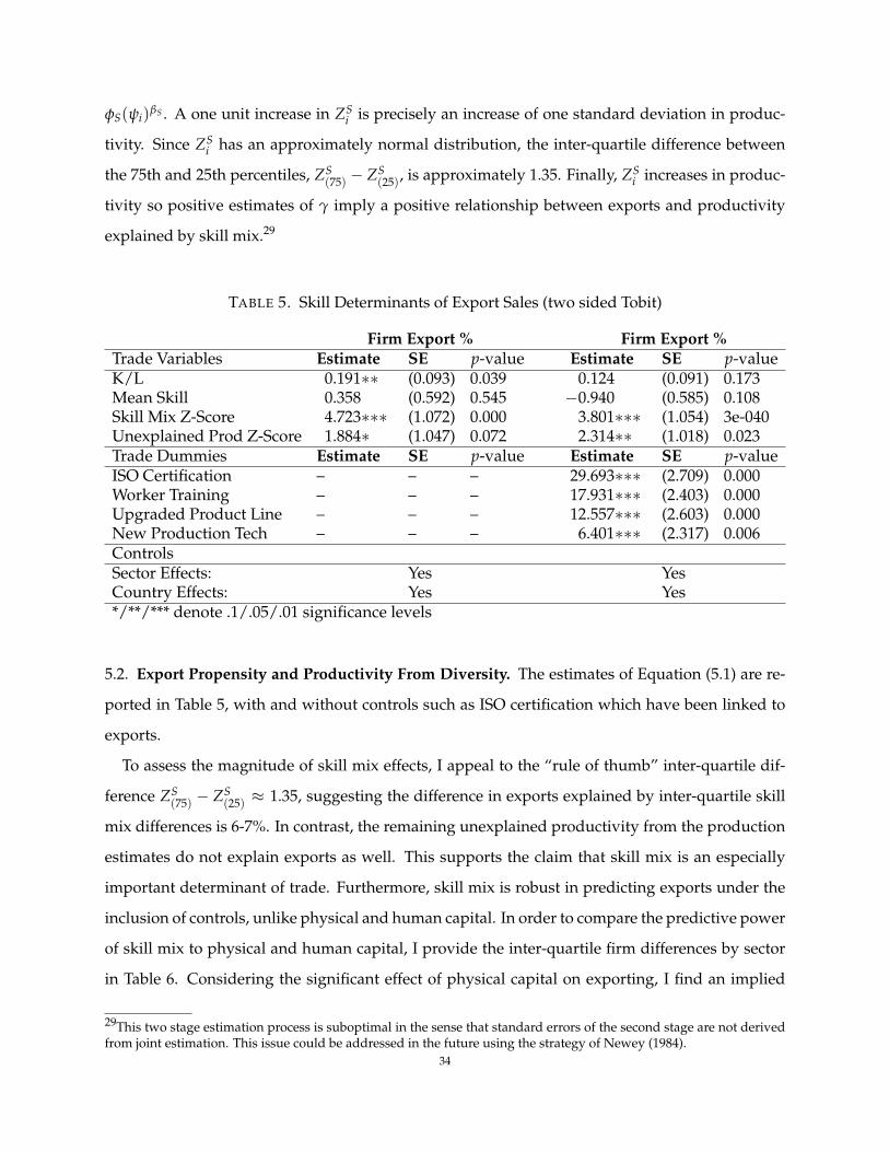
φS(ψi)βS . A one unit increase in ZSi is precisely an increase of one standard deviation in produc-

tivity. Since ZSi has an approximately normal distribution, the inter-quartile difference between

the 75th and 25th percentiles, ZS(75) − ZS

(25), is approximately 1.35. Finally, ZSi increases in produc-

tivity so positive estimates of γ imply a positive relationship between exports and productivity

explained by skill mix.29

TABLE 5. Skill Determinants of Export Sales (two sided Tobit)

Firm Export % Firm Export %Trade Variables Estimate SE p-value Estimate SE p-valueK/L 0.191∗∗ (0.093) 0.039 0.124 (0.091) 0.173Mean Skill 0.358 (0.592) 0.545 −0.940 (0.585) 0.108Skill Mix Z-Score 4.723∗∗∗ (1.072) 0.000 3.801∗∗∗ (1.054) 3e-040Unexplained Prod Z-Score 1.884∗ (1.047) 0.072 2.314∗∗ (1.018) 0.023Trade Dummies Estimate SE p-value Estimate SE p-valueISO Certification – – – 29.693∗∗∗ (2.709) 0.000Worker Training – – – 17.931∗∗∗ (2.403) 0.000Upgraded Product Line – – – 12.557∗∗∗ (2.603) 0.000New Production Tech – – – 6.401∗∗∗ (2.317) 0.006ControlsSector Effects: Yes YesCountry Effects: Yes Yes*/**/*** denote .1/.05/.01 significance levels

5.2. Export Propensity and Productivity From Diversity. The estimates of Equation (5.1) are re-

ported in Table 5, with and without controls such as ISO certification which have been linked to

exports.

To assess the magnitude of skill mix effects, I appeal to the “rule of thumb” inter-quartile dif-

ference ZS(75) − ZS

(25) ≈ 1.35, suggesting the difference in exports explained by inter-quartile skill

mix differences is 6-7%. In contrast, the remaining unexplained productivity from the production

estimates do not explain exports as well. This supports the claim that skill mix is an especially

important determinant of trade. Furthermore, skill mix is robust in predicting exports under the

inclusion of controls, unlike physical and human capital. In order to compare the predictive power

of skill mix to physical and human capital, I provide the inter-quartile firm differences by sector

in Table 6. Considering the significant effect of physical capital on exporting, I find an implied

29This two stage estimation process is suboptimal in the sense that standard errors of the second stage are not derivedfrom joint estimation. This issue could be addressed in the future using the strategy of Newey (1984).

34

export propensity of .7-2.8%, very small compared to the magnitude explained by skill mix. Sim-

ilarly, mean skill shows inter-quartile differences of 1.7-3.5%. Therefore inter-quartile differences

of exporting due to skill mix are more than those from physical and human capital combined. I

conclude that skill diversity is a relatively strong determinant of exports through its effects on firm

productivity.

TABLE 6. Inter-quartile Endowment Differences by Sector

Sector Inte

rqua

rtil

e

K/L

Inte

rqua

rtil

e

Mea

nSk

ill

Inte

rqua

rtil

e

Skil

lMix

Sector Inte

rqua

rtil

e

K/L

Inte

rqua

rtil

e

Mea

nSk

ill

Inte

rqua

rtil

e

Skil

lMix

Agroindustry 14.233 3.775 1.333 Leather 4.9195 2.850 1.309Autos/Components 7.012 2.516 1.521 Metals/Machinery 5.9239 2.255 1.241Beverages 8.198 2.105 1.237 Non-metal/Plastics 9.5572 2.530 1.412Chemicals/Pharma 10.612 3.005 1.407 Other manufacturing 7.2056 1.800 1.295Electronics 6.376 2.300 1.455 Paper 8.6811 1.983 1.429Food 10.563 2.788 1.433 Textiles 7.8246 3.153 1.414Garments 3.616 2.858 1.434 Wood/Furniture 5.3937 2.330 1.369

6. CONCLUSION AND DIRECTIONS FOR FURTHER WORK

This paper has developed a model in which the technical capacity to use diverse workers varies

by sector. The model serves the joint role of extending the theoretical literature and motivating

a structural form for estimation. Theoretically, this paper generates new predictions about how

worker teams are employed and what team members are paid. I provide a new version of the

Rybczynski Theorem: a one percent increase in workers with skills specific to a sector increases

output, but potentially by less than one percent due to worker spillovers. I also provide new

versions of the Stolper-Samuelson theorem. An increase in sector output price will cause a sector

to boom, but superstar effects and entrant workers change the pay structure of the sector. The new

pay structure will increase team wages but may decrease individual wages.

These results suggest growth and trade can exacerbate inequality. In particular, this paper

places emphasis on the role of worker teams formed from asymmetric skill distributions. Since

low and high workers cannot efficiently produce without the other, growth depends on the avail-

able supply of both groups. Wages also hinge on the relative scarcity of low and high skill workers.

Therefore this paper establishes ideas about the structure of production which have fundamental

implications for inequality, among other themes. This suggests further work looking at the link35

between inequality and changes in the size of “skill diversity loving” sectors through growth and

trade. Further work might also consider a political economy framework considering protection as

pro/anti-tariff coalitions can form which cut along both sector and skill lines.

Empirically, I characterize manufacturing sectors by skill mix intensity (diversity or similarity)

helps explain productivity. I find that greater than two thirds of firms in a large cross country sam-

ple belong to sectors where skill mix is an important determinant of productivity. Inter-quartile

productivity differences explained by skill mix are comparable to the magnitude of training and

imported inputs combined, and the magnitude in four sectors is comparable to training, imported

inputs and ISO combined. Furthermore, the majority of sectors best utilize diverse skills, and

theory suggests this explains higher wage inequality through “superstar” wage effects.

Having established a linkage from skill mix to productivity, this paper also evaluates the effect

of productivity differences on exports. I find that differences in skill mix explain intrasector export

variation better than the physical and human capital combined. I conclude that skill diversity is a

relatively good determinant of exports, through its effects on firm productivity. This result clearly

has implications for the human capital content of traded goods. Put together, the results of this

paper show that a more detailed view of human capital, beyond that of a simple average, yields

insights into both productivity and export patterns.

REFERENCES

Acemoglu, D., “Changes in Unemployment and Wage Inequality: An Alternative Theory andSome Evidence,” The American Economic Review, 1999, 89 (5), 1259–1278.

Ackerberg, D., K. Caves, and G. Frazer, “Structural Identification of Production Functions,” Tech-nical Report, UCLA mimeo 2006.

Amemiya, T., “Non-linear regression models,” Handbook of Econometrics, 1983, 1, 333–389.Andersson, F., J. Haltiwanger, M. Freedman, J. Lane, and K. L. Shaw, “Reaching for the Stars:

Who Pays for Talent in Innovative Industries?,” The Economic Journal, 2009, 119 (538), 308–332.Antras, P. and E. Rossi-Hansberg, “Organizations and trade,” 2009.Arnold, J. M., “Productivity Estimation at the Plant Level: A Practical Guide,” Unpublished manu-

script, 2005.Bernard, A. B. and Bradford J. Jensen, “Exceptional exporter performance: cause, effect, or

both?,” Journal of International Economics, 1999, 47 (1), 1–25.Bougheas, Spiros and Raymond Riezman, “Trade and the distribution of human capital,” Journal

of International Economics, November 2007, 73 (2), 421–433.Cameron, A. C. and P. K. Trivedi, Microeconometrics: Methods and Applications, Cambridge Univer-

sity Press, 2005.Costinot, A. and J. Vogel, “Matching and inequality in the world economy,” NBER Working Paper,

2009.Das, S. P., “Vertical Diversity, Communication Gap and Equilibrium Growth,” The BE Journal of

Macroeconomics, 2005, 5 (1), 22.

36

Delacroix, A. G., “Heterogeneous Matching with Transferable Utility: Two Labor Market Appli-cations,” International Economic Review, 2003, 44 (1), 313–330.

Dhingra, Swati and John Morrow, “Is Selection on Firm Productivity a Third Gain from Trade?,”December 2008.

Fernandes, A. M. and A. Pakes, “Factor Utilization in Indian Manufacturing: A Look at the WorldBank Investment Climate Surveys Data,” February 2008.

Goldberg, P. K. and N. Pavcnik, “Distributional Effects of Globalization in Developing Coun-tries,” Journal of Economic Literature, 2007, 45 (1), 39–82.

Grossman, G. M., “The Distribution of Talent and the Pattern and Consequences of InternationalTrade,” Journal of Political Economy, 2004, 112 (1), 209–239.

Grossman, Gene M. and Giovanni Maggi, “Diversity and Trade,” The American Economic Review,2000, 90 (5), 1255–1275.

Halpern, L., M. Koren, and A. Szeidl, “Imported Inputs and Productivity,” Working Paper, April2009.

Hansen, P. and S. Knowles, “Human capital and returns to scale,” Journal of Economic Studies,1998, 25 (2), 118–123.

Hardy, G. H., J. E. Littlewood, and G. Pólya, Inequalities, Cambridge University Press, 1988.Hong, L. and S. E. Page, “Problem Solving by Heterogeneous Agents,” Journal of Economic Theory,

2001, 97 (1), 123–163.Iranzo, S., F. Schivardi, and E. Tosetti, Skill Dispersion and Firm Productivity: An Analysis with

Employer-employee Matched Data, Banca d’Italia, 2006., , and , “Skill dispersion and firm productivity: an analysis with employer-

employee matched data,” Journal of Labor Economics, 2008, 26 (2), 247–285.Jennrich, Robert I., “Asymptotic Properties of Non-Linear Least Squares Estimators,” Annals of

Mathematical Statistics, 1969, 40 (2), 633–643.Jones, Charles I., “Intermediate goods, weak links, and superstars: a theory of economic devel-

opment,” NBER Working Paper, September 2009.Kim, H. Y., “The translog production function and variable returns to scale,” The Review of Eco-

nomics and Statistics, 1992, pp. 546–552.Klump, R., P. Mcadam, and A. Willman, “Factor Substitution and Factor-Augmenting Technical

Progress in the United States: A Normalized Supply-Side System Approach,” The Review ofEconomics and Statistics, 2007, 89 (1), 183–192.

Kmenta, J., “On Estimation of the CES Production Function,” International Economic Review, 1967,8 (2), 180–189.

Kremer, M., “The O-Ring Theory of Economic Development,” Quarterly Journal of Economics, 1993,108 (3), 551–575.

and E. Maskin, “Wage Inequality and Segregation by Skill,” NBER Working Paper, 1996.and , “Globalization and Inequality,” Department of Economics, Harvard University,

Cambridge, MA, 2003.Levinsohn, J. and A. Petrin, “Estimating Production Functions Using Inputs to Control for Unob-

servables,” Review of Economic Studies, 2003, 70 (2), 317–341.Lloyd, P., “Generalizing the Stolper-Samuelson Theorem: A Tale of Two Matrices,” Review of In-

ternational Economics, 2000, 8 (4), 597–613.Loecker, Jan De, “Product differentiation, multi-product firms and estimating the impact of trade

liberalization on productivity,” January 2009.Malinvaud, E., “The consistency of nonlinear regressions,” The Annals of Mathematical Statistics,

1970, 41 (3), 956–969.Mamoon, D. and S. M. Murshed, “Unequal skill premiums and trade liberalization: Is education

the missing link?,” Economics Letters, 2008, (100), 262–266.Manasse, Paolo and Alessandro Turrini, “Trade, wages, and superstars,” Journal of International

37

Economics, June 2001, 54 (1), 97–117.Martins, P. S., “Dispersion in wage premiums and firm performance,” Economics Letters, 2008,

(101), 63–65.Melitz, M., “Estimating Firm-Level Productivity in Differentiated Product Industries,” Harvard

University mimeograph, December 2000.Melitz, M. J., “The Impact of Trade on Intra-Industry Reallocations and Aggregate Industry Pro-

ductivity,” Econometrica, 2003, 71 (6), 1695–1725.and G. I. P. Ottaviano, “Market Size, Trade, and Productivity,” Review of Economic Studies,

2008, 75 (1), 295–316.Moro, A. and P. Norman, “Endogenous Comparative Advantage,” April 2005.Neary, Peter J., The Stolper-Samuelson Theorem, New York: Macmillan Reference, February 2004.Newey, W. K., “A method of moments interpretation of sequential estimators,” Economics Letters,

1984, 14 (2-3), 201–206.Oecd, “South-South Trade: Vital for Development,” Technical Report, OECD August 2006.Ohnsorge, F. and D. Trefler, “Sorting It Out: International Trade with Heterogeneous Workers,”

Journal of Political Economy, 2007, 115 (5), 868–892.Olley, G. S. and A. Pakes, “The Dynamics of Productivity in the Telecommunications Equipment

Industry,” Econometrica, 1996, 64 (6), 1263–1297.Roberts, M. J. and J. R. Tybout, What makes exports boom?, World Bank Publications, 1997.Rockafellar, Tyrrell R., Convex analysis, Vol. 28, Princeton, N.J.: Princeton University Press, 1970.Rosen, S., “The Economics of Superstars,” American Economic Review, 1981, 71 (5), 845–858.Sherstyuk, K., “Efficiency in partnership structures,” Journal of Economic Behavior and Organization,

1998, 36 (3), 331–346.Tsang, H. H. and J. J. Persky, “On the Empirical Content of CES Production Functions,” The

Economic Record, 1975, 51 (4), 539–548.Tybout, J. R., “Manufacturing Firms in Developing Countries: How Well Do They Do, and Why?,”

Journal of Economic Literature, 2000, 38, 11–44.Verhoogen, E. A., “Trade, Quality Upgrading, and Wage Inequality in the Mexican Manufacturing

Sector,” Quarterly Journal of Economics, 2008, 123 (2), 489–530.White, H., “Using Least Squares to Approximate Unknown Regression Functions,” International

Economic Review, 1980, 21 (1), 149–170.Winters, Alan L., Neil Mcculloch, and Andrew Mckay, “Trade Liberalization and Poverty: The

Evidence so Far,” Journal of Economic Literature, 2004, 42 (1), 72–115.Yeaple, Stephen R., “A simple model of firm heterogeneity, international trade, and wages,” Jour-

nal of International Economics, January 2005, 65 (1), 1–20.

APPENDIX A. SUPPLEMENTAL EMPIRICAL DETAILS

A.1. Firm distribution by Sector and Country. This selection of country-year pairs were subject

to the constraints of data availability, and in a few cases when more than one year of suitable data

was available from the same country the most recent set with the largest number of observations

was chosen. Detailed reasons for exclusion are tabulated in the following table.38

TABLE 7. Eligibility of Country-Year datasets

Country/Year: Code: Country/Year: Code: Country/Year: Code: Exclusion Code List:Albania2002 1 Honduras2003 2 Romania2002 1 1 More recent dataAlgeria2002 2 Hungary2002 1 Russia2002 8 available from 2005.Armenia2002 1 India2002 6 Russia2005 8 2 Incomplete, missing, orAzerbaijan2002 3 Indonesia2003 2 Senegal2003 6 incompatible education data.Azerbaijan2005 3 Ireland2005 5 Serbia&Mont2002 1 3 Incomplete or missingBangladesh2002 2 Kazakhstan2002 1 Serbia2003 1 labor costs.Belarus2002 1 Kenya2003 6 Slovakia2002 5 4 Incomplete or missingBiH2002 4 Kosovo2003 4 Slovakia2005 5 asset data.BiH2005 4 Kyrgyzstan2002 4 Slovenia2002 4 5 Censored for highBulgaria2002 1 Kyrgyzstan2005 4 Slovenia2005 4 GDP/capita.Bulgaria2004 1 Latvia2002 1 SouthKorea2005 3 6 Missing ISO or productionChina2002 2 Lithuania2002 4 Spain2005 5 upgrading data.China2003 2 Lithuania2005 4 SriLanka2004 6 7 Included separateCroatia2002 1 Malawi2005 2 Syria2003 2 survey from same year.Czech2002 5 Mali2003 4 Tajikistan2002 1 8 Excluded as Russian economyCzech2005 5 Moldova2002 1 Tajikistan2003 1 reorganizing from USSR,Ecuador2003 2 Moldova2003 1 Tanzania2003 2 results robust in inclusion.Eritrea2002 2 Montenegro2003 1 Thailand2004 2Estonia2002 1 Nicaragua2003 2 Turkey-b2005 7Ethiopia2002 2 Pakistan2002 6 Turkey2002 1FYROM2002 1 Peru2002 6 Uganda2003 3Georgia2002 1 Philippines2003 2 Ukraine2002 1Germany2005 5 Poland2002 1 Uzbekistan2002 4Greece2005 3 Poland2003 1 Uzbekistan2005 4Guatemala2003 2 Portugal2005 3 Vietnam-b2005 7

The distribution of firms by sector and country is presented in Table 8. In order to facilitate het-

eroskedasticity by sector-country pairs, sector-country pairs containing exactly one observation

were dropped from the sample, making the minimum number of observations two for each pair.39

TABLE 8. Distribution of Firms by Country and Sector

Country Year Agr

oind

ustr

y

Aut

os/C

ompo

nent

s

Bev

erag

es

Che

mic

als/

Phar

ma

Elec

tron

ics

Food

Gar

men

ts

Leat

her

Met

als/

Mac

hine

ry

Non

-met

al/P

last

ics

Oth

erM

anuf

actu

ring

Pape

r

Text

iles

Woo

d/Fu

rnit

ure

Cou

ntry

Tota

ls

Albania 2005 0 0 8 3 0 5 5 0 4 2 0 0 0 4 31Armenia 2005 0 0 70 3 0 13 9 0 23 6 0 4 3 6 137Belarus 2005 0 0 0 0 0 0 0 0 6 6 3 0 0 3 18Benin 2004 13 0 0 5 0 0 0 0 8 0 0 0 0 25 51Brazil 2003 0 118 0 68 57 103 405 154 157 0 0 0 96 275 1433Bulgaria 2005 0 0 6 2 0 2 3 0 7 2 0 0 5 3 30Cambodia 2003 3 0 0 0 0 0 11 0 0 0 0 0 0 0 14Chile 2004 39 0 16 85 0 134 0 0 119 0 0 40 0 71 504CostaRica 2005 0 0 4 0 2 16 8 2 19 40 19 2 10 12 134Croatia 2005 0 0 3 2 0 0 0 0 6 4 0 2 0 2 19Egypt 2004 0 8 0 48 0 95 80 19 107 119 25 0 85 31 617ElSalvador 2003 0 0 0 3 0 5 3 0 5 0 0 0 0 0 16Estonia 2005 0 0 3 0 0 0 4 0 4 2 0 3 2 4 22FYROM 2005 0 0 5 0 0 2 0 0 5 0 0 0 0 2 14Georgia 2005 0 0 8 0 0 2 0 0 2 0 0 0 2 0 14Guyana 2004 0 0 0 3 0 51 6 0 0 0 0 0 5 28 93Hungary 2005 0 0 6 0 0 14 23 2 110 7 0 7 5 3 177Kazakhstan 2005 0 0 85 0 0 3 16 0 46 4 0 4 0 0 158Kyrgyzstan 2003 0 0 16 3 0 14 12 0 4 6 0 0 7 2 64Latvia 2005 0 0 2 0 0 0 4 0 3 0 0 2 0 4 15Lithuania 2004 0 0 0 0 0 22 0 0 0 0 0 0 33 9 64Madagascar 2005 0 0 0 5 0 10 11 2 4 4 12 2 4 10 64Mauritius 2005 0 0 3 5 0 12 0 0 4 0 3 10 14 4 55Moldova 2005 0 0 39 0 0 5 16 0 16 2 3 2 0 5 88Morocco 2004 0 0 0 56 30 60 319 76 17 70 0 3 151 3 785Oman 2003 0 0 0 3 0 5 0 0 9 12 4 2 0 2 37Poland 2005 0 0 8 0 0 32 46 0 78 3 0 4 4 3 178Romania 2005 0 0 36 9 0 29 65 2 62 4 0 5 5 6 223Serb&Mont 2005 0 0 6 0 0 2 0 0 5 0 0 2 2 0 17SouthAfrica 2003 0 0 0 35 7 44 20 7 100 38 72 11 17 69 420Tajikistan 2005 0 0 4 0 0 4 4 0 5 6 0 6 6 0 35Turkey 2005 0 0 0 32 6 84 48 4 107 38 3 2 56 6 386Ukraine 2005 0 0 13 3 0 3 9 4 13 4 11 6 4 9 79Uzbekistan 2003 0 0 0 0 0 8 9 0 0 0 0 0 0 0 17Vietnam 2005 0 0 2 23 5 82 34 8 95 83 60 31 34 85 542Zambia 2002 71 0 0 18 0 0 0 0 19 0 0 7 17 4 136Sector Totals 126 126 343 414 107 861 1170 280 1169 462 215 157 567 690 6687

A.2. Controlling for the sales effects of exporting. Ideally, the data set would include production

information that differentiates the use of inputs for domestic and foreign use. Of course, many40

inputs are used in both domestic and foreign production activities, so the true counterfactuals of

exporting are not directly observable. I therefore impose structure on the domestic and foreign

decomposition of revenues to control for market segmentation.

Suppose firm i produces a quality adjusted quantity qi, of which a fraction Xi is sold to foreign

markets at price pXi , and the remainder is sold domestically at price pD

i . Then value added sales

Yi are given by Equation (A.1)

Yi = Xi · [pXi − cX

i ]qi + (1− Xi) · [pDi − cD

i ]qi(A.1)

where cXi and cD

i are foreign and domestic material input costs. Defining the foreign (MXi ) and

domestic (MDi ) markups in the usual way by MX

i ≡ (pXi − cX

i )/cXi and MD

i ≡ (pDi − cD

i )/cDi ,

rewrite Equation (A.1) as

Yi = (pDi − cD

i )qi︸ ︷︷ ︸Value added sales at

domestic prices and input costs

· 1 +MX

i (cXi /cD

i )−MDi

MDi

Xi︸ ︷︷ ︸Export weight to account for

foreign markups and input costs

(A.2)

Equation (A.2) shows value added sales decomposed into domestic value added sales times an

export weight that depends on markups and input costs. Introducing the shorthand

Mi ≡[

MXi (cX

i /cDi )−MD

i

]/MD

i

and taking logs, Equation (A.2) becomes

ln Yi ≈ ln(pDi − cD

i )qi + MiXi

where the approximation is the commonly used fact that ln(1 + x) ≈ x for small values of x. This

approximation halves the number of non-linear parameters to recover. Although the individual

elements of MiXi are not identified, Xi is observed. Assuming the term Mi does not vary across

some grouping, (as would be implied by constant markups within the grouping and cXi /cD

i fixed),

Mi can be used to control for the sales effects of exporting. In what follows, I assume Mi ≡ MS for

all firms i in sector S in order to focus on within-sector differences.30 Since the firms considered

30Constant markups for both exporting and domestic production are, for example, consistent with Melitz (2003), butno longer hold once that model is modified to allow for scale effects as in Melitz and Ottaviano (2008). For a concisesummary and comparison of these models see Dhingra and Morrow (2008).

41

produce in developing countries, generally one should expect MS ≥ 0. This is because of the high

value exported to the economic North, suggesting MXS ≥ MD

S (see OECD (2006)) and because of

potentially higher costs for “export quality” goods (cXS ≥ cD

S ).

A.3. Translog production estimates. After adding the labor augmenting effect of skill mix, the

translog specification implies

ln F(K, φ(ψi) · L) ≡ αS ln Ki + βS ln (φ(ψi)Li) + ∑i,j

γij ln Ki ln(φ(ψi)Lj

)(A.3)

Estimates are reported in Table 9.

TABLE 9. Translog production estimates

Dependent Var: Value Added SalesControls Estimate SE p-value Other ControlsUpgraded Products 0.0357*** (0.0124) 0.0019 Sector-Year &New Prod Tech 0.0169* (0.012) 0.0797 Country DummiesISO Certification 0.0379*** (0.0163) 0.0100Worker Training -0.0104 (0.0122) 0.1973 Summary Stats% Imported Inputs 0.0856*** (0.0159) 0.0000 Obs: 6687Foreign Own 0.0633*** (0.0194) 5e-040 R2: 0.899Production and Capital Labor Markup Capital· CES Param (ρS)Markups (αS) (βS) (MS) Capital2 Labor2 Labor Estimate p-valueAgroindustry 0.3562* 0.2956 -.1255 .0025 .0351 -.0031 1.5585 0.2664Autos & comp -0.2343 1.4013*** .6052 .0730*** .0153 -.1163*** 0.7720* 0.0906Beverages 0.2204* 0.7253*** -.0427 .0743*** .0580*** -.1345*** 0.6019*** 0.0000Chem/Pharma 0.0185 1.0526*** -.0419 .0780*** .0871*** -.1702*** 0.7168*** 0.0030Electronics 0.0249 0.6666*** .0241 .0292 .0269 -.0326 0.6947** 0.0205Food 0.1557** 0.9155*** .0755 .0586*** .0557*** -.1244*** 1.5216** 0.0115Garments 0.0924* 1.0049*** .0834** .0835*** .1085*** -.1963*** 1.0753 0.1760Leather 0.0276 1.1396*** .1685** .0473** .0293 -.0929** 0.8835 0.1166Metals/Machinery -0.0103 0.9904*** -.0233 .0922*** .0912*** -.1811*** 0.8871* 0.0747Non-metal/Plastics -0.3054*** 1.0338*** -.2751*** .0709*** -.0319* -.0465* 0.6364*** 0.0000Other manufact. 0.3653** 0.6903*** -.0796 .0070 .0049 -.0197 0.7089*** 0.0086Paper -0.7113*** 1.7950*** .2883*** .1995*** .2129*** -.4195*** 0.7707*** 0.0058Textiles 0.1809** 1.0182*** .0829* .0417*** .0291** -.0914*** 1.0058 0.4711Wood and furniture 0.0474 1.0394*** .0705 .0646*** .0712*** -.1426*** 0.8126*** 0.0024*/**/*** denote .1/.05/.01 Significance levels

This specification coincides with that of the main text, with the exception that firm size is not

included as a control since the specification (A.3) already captures much variation in possible scale

effects. Note that the estimates are somewhat inefficient as the share equations associated with this

specification were not used in estimation, see Kim (1992).42

APPENDIX B. PROOFS

This section of the appendix includes most proofs from the main text. The construction of

wages as those which support the efficient competitive equilibrium is considerably involved and

available from the author upon request.

Lemma. If Φ has finite expectation then the value of all production in the economy is bounded.

Proof. For the result it is necessary to show that for all admissible allocations A ≡ (q, M(q), ι(q))of workers to firms that

supA

∫pι(q)Fι(q)(q, M(q))dΦ < ∞(B.1)

Since the integrand in equation (B.1) is always positive, for the result it is sufficient to show it holdsfor N + 1 different economies with technologies Fi and the entire distribution of skill to allocate.Formally, it is sufficient to show for the allocations Ai, i = 0, . . . , N which employ all workers ineach sector i that

supAi

∫piFi(q, M(q))dΦ < ∞ ∀i = 0, . . . , N(B.2)

Since each Fi is increasing in each argument and is homogeneous of degree one, piFi(q, M(q)) ≤max{q, M(q)} · piFi(1, 1) ≤ (q + M(q)) · piFi(1, 1). Thus for equation (B.2) to hold, since the termspiFi(1, 1) are irrelevant for boundedness, it is enough that

supAi

∫(q + M(q))dΦ < ∞ ∀i = 0, . . . , N(B.3)

Examining equation (B.3),∫

qdΦ is the mean of Φ which is assumed finite so showing supM

∫M(q)dΦ <

∞ will prove the result. I claim in fact that∫

M(q)dΦ =∫

qdΦ for any admissible M. This followsfrom the allocative nature of M which requires

∫{q: M(q)∈[a,b]} 1dΦ = Φ(b)−Φ(a) so in particular

for any integers j and K,∣∣∣∣∫ (j+1)/K

j/KqdΦ−

∫{q: M(q)∈[ j

K , j+1K ]}

M(q)dΦ∣∣∣∣ ≤ [

j + 1K− j

K]∣∣∣∣∫ (j+1)/K

j/K1dΦ−

∫{q: M(q)∈[ j

K , j+1K ]}

1dΦ∣∣∣∣

≤ [Φ((j + 1)/K)−Φ(j/K)]/K

Summing both sides over j implies∣∣∣∣∫ ∞

0qdΦ−

∫{q: M(q)<∞}

M(q)dΦ∣∣∣∣ ≤ lim

j→∞Φ((j + 1)/K)/K = 1/K

and letting K → ∞ shows∫

M(q)dΦ =∫

qdΦ which is finite, proving the result. �

Lemma (CES Ranking). Suppose each Fi is CES, specifically Fi(q, q′) ≡ Ai(qρi + q′ρi)1/ρi . Then Si � Sjif and only if ρi > ρj so CES production technologies imply a complete diversity ranking.

Proof. It is clear that a necessary condition for Si � Sj is ρi 6= ρj. Some algebra along withthe differentiability and homogeneity of each Fi shows that another necessary condition is thatFi

2(1, z)/Fj2(1, z) ≥ Fi(1, z)/Fj(1, z) for all z > 1 or rather

Aizρi−1(1 + zρi)(1/ρi)−1

Ajzρj−1(1 + zρj)(1/ρj)−1≥ Ai(1 + zρi)1/ρi

Aj(1 + zρj)1/ρj

43

which holds iff zρi /(1 + zρi) ≥ zρj /(1 + zρj). Since x/(1 + x) is strictly increasing for x > 0, theinequality holds iff zρi ≥ zρj . Since ρi 6= ρj equality cannot hold and since z > 1 this holds iffρi > ρj. Working backwards, ρi > ρj is sufficient for Si � Sj, giving the result. �

Proposition. Under Assumption 1, any equilibrium allocation exhibits skill ratios {t̂i}, increasing in i,where if (q, M(q)) are assigned to Si then M(q)/q ∈

[t̂i, t̂i+1

). The ratios are fixed for i > 1 by

piFi(1, t̂i) = pi−1Fi−1(1, t̂i)

Proof. First consider any worker team (q, M(q)) and consider assigning the team to either Si or Sj

with j > i. Note that for any fixed wage structure, π j(q, M(q)) ≥ πi(q, M(q)) iff pjFj(q, M(q)) ≥piFi(q, M(q)) iff pjFj(1, x) ≥ piFi(1, x) where x ≡ M(q)/q. Therefore, conditional on wages w(q),the most profitable assignment depends on the skill ratio x. Assumption 1 implies Fi(1, x) andFj(1, x) cross at most once, and they cross at least once31, so let χ(i, j) denote the skill ratio atwhich the crossing occurs. Since pjFj(1, x)/piFi(1, x) is increasing by Assumption 1, it followsthat pjFj(1, x) ≥ piFi(1, x) iff x ≥ χ(i, j). Working backwards to the profit conditions for fixedwages, we conclude

π j(q, M(q)) ≥ πi(q, M(q)) iff M(q)/q ≥ χ(i, j)

Now consider which skill ratios may be assigned to SN . Since SN � Sj for any j, it follows thatif M(q)/q ≥ maxi χ(i, N), SN is the most profitable sector to employ (q, M(q)). Conversely, ifM(q)/q < maxi χ(i, N) there is some Sj which is more profitable to employ (q, M(q)). ThereforeSN consists of the most diverse teams where M(q)/q ≥ maxi χ(i, N). Proceeding recursively forSN−1 (which satisfies SN−1 � Sj for any j < N), (q, M(q)) is most profitably employed in SN−1 iffM(q)/q ∈ [maxi<N−1 χ(i, N − 1), maxi<N χ(i, N)). Continuing in this fashion produces the skillratio cutoffs {t̂i} as promised where by convention t̂N+1 ≡ ∞.

Finally, the recursive nature of assignment fixes each t̂i to where “Si−1 crosses Si”, namelypiFi(1, t̂i) = pi−1Fi−1(1, t̂i). This is exactly equivalent to t̂i = χ(i − 1, i). To see the result, sup-pose t̂i = χ(k, i) > χ(i− 1, i) so piFi(1, t̂i) > pi−1Fi−1(1, t̂i) and

1 =piFi(1, t̂i)pkFk(1, t̂i)

=i

∏j=k+1

pjFj(1, t̂i)pj−1Fj−1(1, t̂i)

>piFi(1, t̂i)

pi−1Fi−1(1, t̂i)︸ ︷︷ ︸>1

i−1

∏j=k+1

pjFj(1, t̂j)pj−1Fj−1(1, t̂j)︸ ︷︷ ︸

=1

(B.4)

where the inequality follows from the fact that t̂i > t̂j for j < i. Equation (B.4) yields a contradic-tion and it holds that piFi(1, t̂i) = pi−1Fi−1(1, t̂i) for each i. �

Proposition. The wage schedule w(q) has the following properties:(1) w(q) is strictly increasing and convex.(2) w(q) is bounded below by the S0 shadow wages w0q.(3) w′(q) is increasing where defined, and elsewhere limq→x− w′(q) ≤ limq→x+ w′(q).

Proof. First Claim: That w(q) is strictly increasing is obvious from the form. Convexity followsfrom the third claim combined with Theorem 24.2 of (Rockafellar, 1970) by pasting across sectors.

Second Claim: The result clearly holds for workers in S0 so consider workers in the sectors{Si}i≥1. First note that for i ≥ 1, Fi

12 ≤ 0 and given that Fi is homogeneous of degree one impliesFi

11 ≥ 0. Second, since at least some firms produce in the S0 sector, efficiency implies that for alli, piFi(1, 1) ≤ p0F0(1, 1) = 2w0. Using these facts, for any worker of skill q which is below themedian of Φ it holds that

Fi1(q, M(q)) = Fi

1(q/M(q), 1) ≤ Fi1(1, 1) = Fi(1, 1)/2 ≤ w0/pi(B.5)

31Otherwise one technology is always dominated at current prices, so it may be omitted without loss of generality.44

We conclude that piFi1(q, M(q)) ≤ w0. This implies for any q below the median employed in

{Si}i≥1 wages are bounded below by

w(q) = w(t0)−∫ ti−1

qpiFi

1(s, M(s))ds ≥ w(ti−1)−∫ ti−1

qw0ds = w(ti−1)− w0[ti−1 − q](B.6)

Consequently, if q is employed in S1, using the fact that w(t0) = w0t0, Equation (B.6) impliesw(q) ≥ w0q. Proceeding inductively for q below the median, suppose w(q) ≥ w0q for sector Si−1so for Si, Equation (B.5) implies

w(q) ≥ w(ti−1)− w0[ti−1 − q] ≥ w0ti−1 − w0[ti−1 − q] = w0q(B.7)

Therefore by induction, Equation (B.7) implies w(q) ≥ w0q for all q below the median of Φ. Asimilar method applies to q above the median of Φ by exploiting the analogous inequality ofEquation (B.5) using Fi

2.Third Claim: For q not at a cusp {ti} or {M(ti)} this follows from Fi

11, Fi22 ≥ 0 for q in {Si}i≥1

and from w′(q) = w0 for q in S0. Now suppose q = ti for some i. For δ > 0,

w′(ti − δ) = pi+1Fi+11 (ti − δ, M(ti − δ)) and w′(ti + δ) = piFi

1(ti + δ, M(ti + δ))(B.8)

Therefore it is sufficient to show that

limδ→0−

pi+1Fi+11 (ti − δ, M(ti − δ)) ≤ lim

δ→0+piFi

1(ti + δ, M(ti + δ))

and since each Fi1 is continuous this inequality holds if pi+1Fi+1

1 (ti, M(ti)) ≤ piFi1(ti, M(ti)). Since

Si+1 � Si, by definition ∂∂x

pi+1Fi+1(1,x)pi Fi(1,x) ≥ 0. This implies through homogeneity that

pi+1Fi+12 (y, z)

pi+1Fi+1(y, z)≥ piFi

2(y, z)piFi(y, z)

∀z/y ≥ t̂i+1(B.9)

Also by definition, M(ti)/ti = t̂i+1 and pi+1Fi+1(ti, M(ti)) = piFi(ti, M(ti)) so letting y = tiand z = M(ti) in Equation (B.9) the denominators cancel and it holds that pi+1Fi+1

2 (ti, M(ti)) ≥piFi

2(ti, M(ti)). Homogeneity then implies pi+1Fi+11 (ti, M(ti)) ≤ piFi

1(ti, M(ti)) as desired. Thecusps {M(ti)} can be shown similarly. �

Lemma. Let Φ and Φ̃ be two skill distributions and t0, t̃0 be the respective skill cutoffs in equilibrium.Consider a Skill Shock from Φ to Φ̃. Then:

(1) Following a DSS the mass of workers in S1 increases.(2) Following a HSS, t̃0 ≥ t0 and M(t̃0) ≥ M(t0) (and S1 workers increase).(3) Following a LSS, t̃0 ≤ t0 and M(t̃0) ≤ M(t0) (and S1 workers increase).

Proof. I first show Claim 2. Let M̃ denote the equilibrium skill pairings under Φ̃. Under a HSS,by assumption Φ̃(t0) = Φ(t0) and Φ̃(M(t0)) ≤ Φ(M(t0)) so that Φ̃(t0) + Φ̃(M(t0)) ≤ 1. Inequilibrium necessarily M(t0)/t0 = M̃(t̃0)/t̃0 = t̂1 since the {t̂i} are fixed by prices and pro-duction technologies that are independent of the skill distribution. Therefore Φ̃(t0) + Φ̃(t̂1t0) =Φ̃(t0) + Φ̃(M(t0)) ≤ 1 which implies

Φ̃(t0) + Φ̃(t̂1t0) ≤ 1 = Φ̃(t̃0) + Φ̃(t̂1 t̃0)

and since Φ̃ is increasing, conclude t̃0 ≥ t0. Therefore Φ̃(t̃0) ≥ Φ̃(t0) = Φ(t0) so the mass ofworkers employed in S1 under Φ̃ is larger than under Φ as claimed. Claim 3 then follows by asymmetric argument. Claim 1 follows by decomposing any DSS into a HSS for changes above themedian and a LSS for changes below the median and applying Claims 2 and 3 in succession. �

Proposition. Increases in sector specific skills increase sector output. Absent spillovers, output is magni-fied due to more efficient worker sorting.

45

Proof. Let Υ denote the combined skill distribution of Φ and Ψ, namely the skill distribution withmass L + P and (proper) distribution λΦ + (1− λ)Ψ where λ ≡ L

L+P . Also let MΦ denote thematch function Φ generates in isolation and similarly MΨ and MΥ. I first claim

min{MΦ, MΨ} ≤ MΥ ≤ max{MΦ, MΨ}(B.10)

To see this, note that by definition

Φ + Φ ◦min{MΦ, MΨ} ≤ 1 and Ψ + Ψ ◦min{MΦ, MΨ} ≤ 1

and therefore for any λ ∈ [0, 1]

λΦ + (1− λ)Ψ + [λΦ + (1− λ)Ψ] ◦min{MΦ, MΨ} ≤ 1

which with Υ + Υ ◦MΥ = 1 shows min{MΦ, MΨ} ≤ MΥ and similarly MΥ ≤ max{MΦ, MΨ} soEquation (B.10) holds. Investigation shows there are no worker spillovers iff

MΦ(ti−1)ti−1

≤ MΥ(ti−1)ti−1

andMΥ(ti)

ti≤ MΦ(ti)

ti(B.11)

Equation (B.10) implies that Equation (B.11) holds so long as

MΦ(ti−1) ≤ MΨ(ti−1) and MΨ(ti) ≤ MΦ(ti)(B.12)

Since the support of Ψ is on [ti, ti−1] ∪ [MΦ(ti−1), MΦ(ti)], clearly MΨ(ti) ≤ MΦ(ti). Since thereare equal masses of low and high skill workers in Ψ, limx−→.5+ Ψ−1(x) ≥ MΦ(ti−1) so Equation(B.12) holds. Therefore there are no worker spillovers. Magnification follows from the optimalityof MΥ. �

Proposition. If the skill distribution is symmetric then the indirect Stolper-Samuelson effect dominatesthe direct effect.

Proof. The indirect effect dominates when for any i ≥ 1 and q ∈ (ti, ti−1]:∫ ti−1

qFi

1(s, M(s))ds ≤ Fi(ti−1, M(ti−1)) ·M(ti−1)/ti−1

M(ti−1)/ti−1 + 1(B.13)

Noting that for any s, Fi1(s, M(s)) = Fi

1(s/M(s), 1) and Fi11 ≥ 0, it follows Fi

1(s, M(s)) ≤ Fi1(ti−1, M(ti−1)).

Therefore ∫ ti−1

qFi

1(s, M(s))ds ≤∫ ti−1

qFi

1(ti−1, M(ti−1))ds ≤ Fi1(ti−1, M(ti−1))ti−1(B.14)

Using the fact that Fi2(x, y) = Fi

1(y, x) it is also clear that

Fi(ti−1, M(ti−1)) = Fi1(ti−1, M(ti−1))ti−1 + Fi

2(ti−1, M(ti−1))M(ti−1)

≥ Fi1(ti−1, M(ti−1)[ti−1 + M(ti−1)](B.15)

Applying the inequalities of Equation (B.14) to the LHS of Equation (B.13) and Equation (B.15) tothe RHS of Equation (B.13) it is sufficient for the result that

Fi1(ti−1, M(ti−1))ti−1 ≤ Fi

1(ti−1, M(ti−1)[ti−1 + M(ti−1)]M(ti−1)

M(ti−1) + ti−1

which clearly holds. �

46