johns hopkins university

Johns Hopkins University - Fall 2003 Phylogenetics & Computational Genomics - 410.640.71

Lecture #6

Week6: Intro to Phylogenetic Reconstruction& Distance Based Methods

• introduction to phylogenies• distance based methods• phylogeny exercises

Phylogeny Objectives

1 - understand the essence of phylogenies (definition of terms)2 - understand distance based methods of phylogenetic reconstruction3 - should be able to use various software packages to reconstruct and view phylogenies: ClustalX, MEGA, DAMBE, Treeview

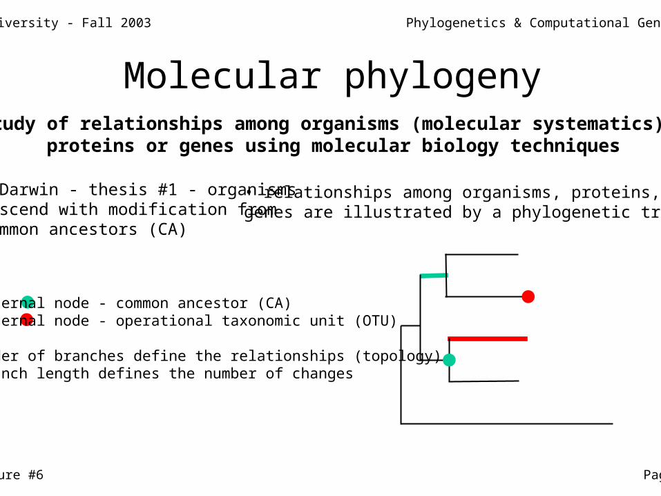
study of relationships among organisms (molecular systematics), proteins or genes using molecular biology techniques

Molecular phylogeny

• Darwin - thesis #1 - organisms descend with modification from common ancestors (CA)

internal node - common ancestor (CA)external node - operational taxonomic unit (OTU)

order of branches define the relationships (topology)branch length defines the number of changes

• relationships among organisms, proteins, genes are illustrated by a phylogenetic tree

Lecture #6


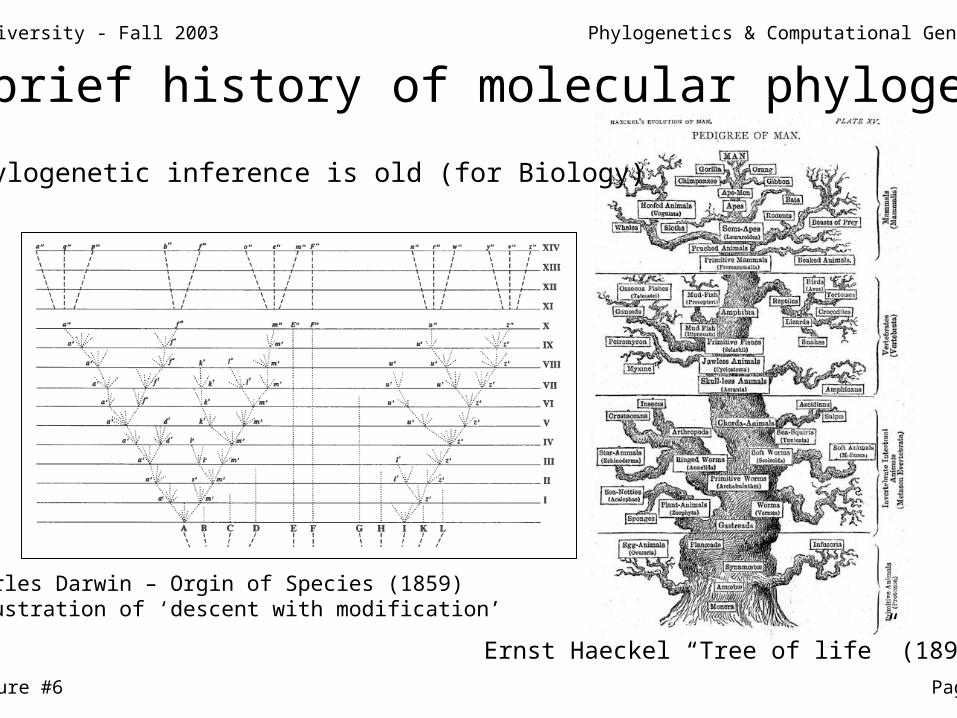
A brief history of molecular phylogeny

Lecture #6


• phylogenetic inference is old (for Biology)

Ernst Haeckel “Tree of life” (1891)

Charles Darwin – Orgin of Species (1859)Illustration of ‘descent with modification’

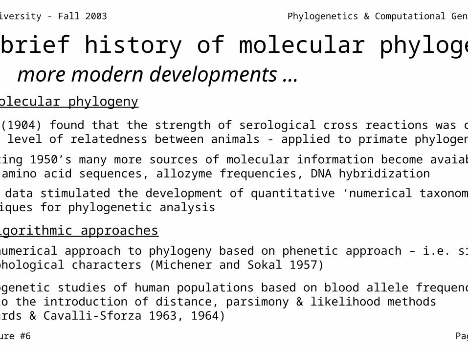
A brief history of molecular phylogeny

• Nuttall (1904) found that the strength of serological cross reactions was correlated with the level of relatedness between animals - applied to primate phylogeny

Lecture #6


Molecular phylogeny

Algorithmic approaches

more modern developments …

• starting 1950’s many more sources of molecular information become avaiable: e.g. amino acid sequences, allozyme frequencies, DNA hybridization

• these data stimulated the development of quantitative ‘numerical taxonomy’ techniques for phylogenetic analysis

• first numerical approach to phylogeny based on phenetic approach – i.e. similarity of morphological characters (Michener and Sokal 1957)

• phylogenetic studies of human populations based on blood allele frequencies led to the introduction of distance, parsimony & likelihood methods (Edwards & Cavalli-Sforza 1963, 1964)

A brief history of molecular phylogeny …

Lecture #6


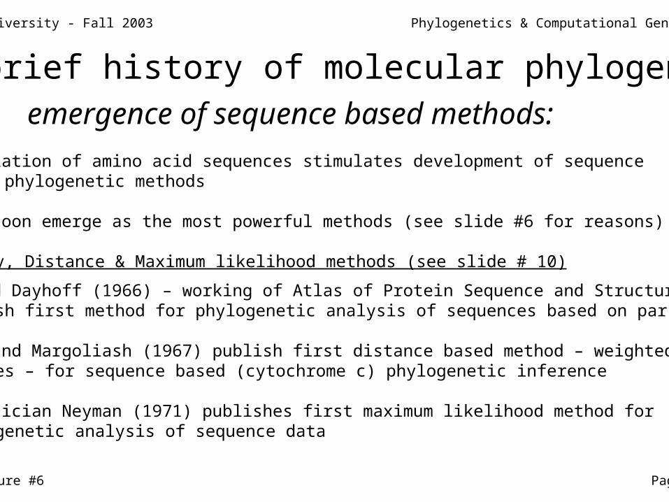
emergence of sequence based methods:

accumulation of amino acid sequences stimulates development of sequence based phylogenetic methods

these soon emerge as the most powerful methods (see slide #6 for reasons)

Parsimony, Distance & Maximum likelihood methods (see slide # 10)

Eck and Dayhoff (1966) – working of Atlas of Protein Sequence and Structure – publish first method for phylogenetic analysis of sequences based on parsimony

Fitch and Margoliash (1967) publish first distance based method – weighted least squares – for sequence based (cytochrome c) phylogenetic inference

Statistician Neyman (1971) publishes first maximum likelihood method for phylogenetic analysis of sequence data

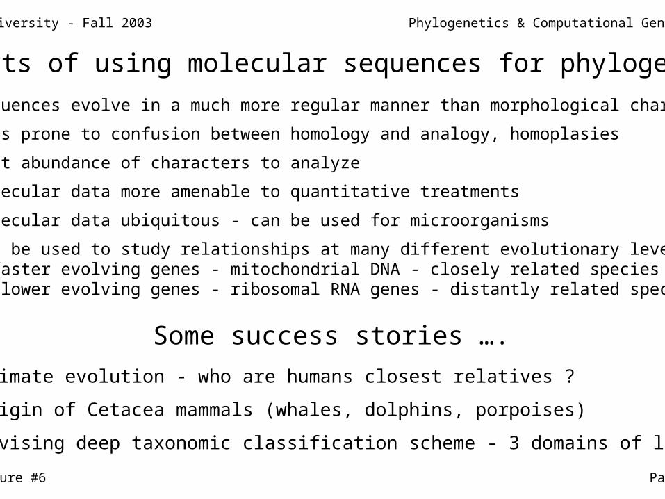
Benefits of using molecular sequences for phylogenetics

1 - sequences evolve in a much more regular manner than morphological characters

2 - less prone to confusion between homology and analogy, homoplasies

3 - vast abundance of characters to analyze

4 - molecular data more amenable to quantitative treatments

5 - molecular data ubiquitous - can be used for microorganisms

6 - can be used to study relationships at many different evolutionary levels faster evolving genes - mitochondrial DNA - closely related species slower evolving genes - ribosomal RNA genes - distantly related species

Some success stories ….

• primate evolution - who are humans closest relatives ?

• origin of Cetacea mammals (whales, dolphins, porpoises)

• revising deep taxonomic classification scheme - 3 domains of life

Lecture #6


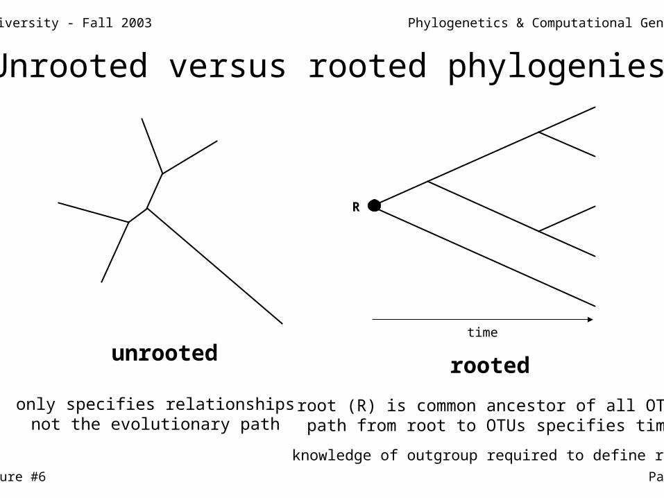
unrootedrooted

R

only specifies relationshipsnot the evolutionary path

root (R) is common ancestor of all OTUspath from root to OTUs specifies time

knowledge of outgroup required to define root

time

Unrooted versus rooted phylogenies

Lecture #6


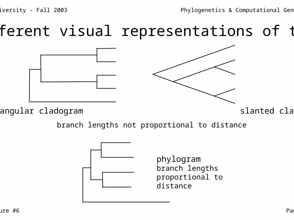
Different visual representations of trees

phylogrambranch lengthsproportional todistance

rectangular cladogram slanted cladogram

branch lengths not proportional to distance

Lecture #6


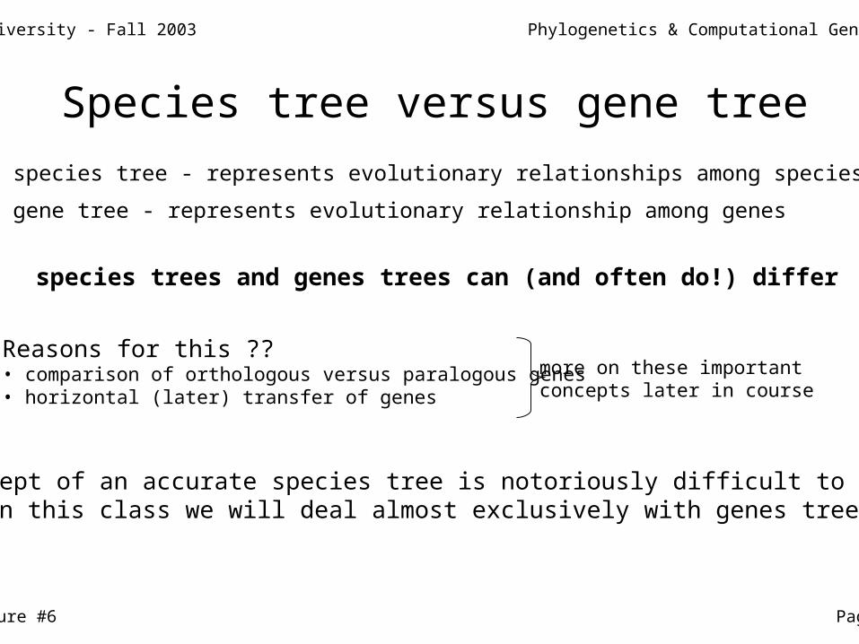
Species tree versus gene tree

species tree - represents evolutionary relationships among species

gene tree - represents evolutionary relationship among genes

species trees and genes trees can (and often do!) differ

Reasons for this ??• comparison of orthologous versus paralogous genes• horizontal (later) transfer of genes

the concept of an accurate species tree is notoriously difficult to pin downin this class we will deal almost exclusively with genes trees

more on these important concepts later in course

Lecture #6


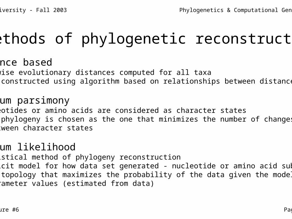
Distance based• pairwise evolutionary distances computed for all taxa• tree constructed using algorithm based on relationships between distances

Maximum parsimony• nucleotides or amino acids are considered as character states• best phylogeny is chosen as the one that minimizes the number of changes between character states

Maximum likelihood• statistical method of phylogeny reconstruction• explicit model for how data set generated - nucleotide or amino acid substitution• find topology that maximizes the probability of the data given the model and the parameter values (estimated from data)

Methods of phylogenetic reconstruction

Lecture #6


Lecture #6


Phylogenetic inference

1 – sequences change as they evolve from a common ancestor over time

2 – a group of related sequences retains information (incomplete) about the evolutionary history that unites them – based on the pattern of changes

3 – phylogeny is estimation, make the best estimate about evolutionary historygiven the incomplete information in the sequences being analyzed

4 – information about the past is not available, only extant sequences

5 – therefore any evolutionary scenario (i.e. phylogeny) can be postulated to explain the changes in the sequences being analyzed

6 – must have some way to discriminate among the (many!) possible phylogenies

n

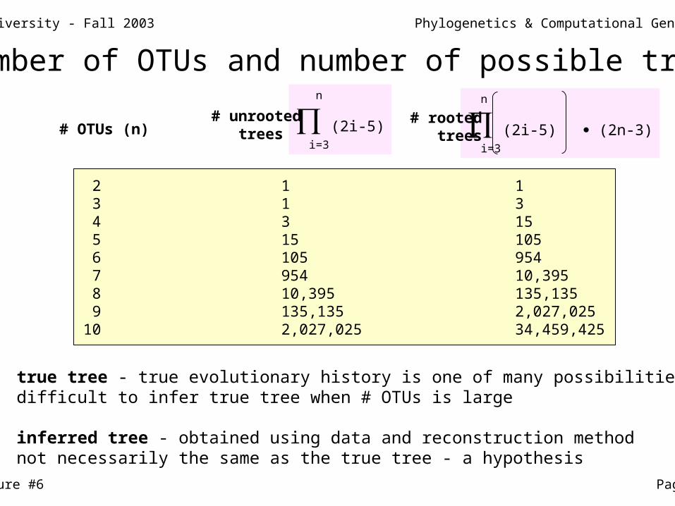
(2i-5) (2n-3) i=3

Number of OTUs and number of possible trees

# rooted trees

2 1 1 3 1 3 4 3 15 5 15 105 6 105 954 7 954 10,395 8 10,395 135,135 9 135,135 2,027,02510 2,027,025 34,459,425

true tree - true evolutionary history is one of many possibilitiesdifficult to infer true tree when # OTUs is large

inferred tree - obtained using data and reconstruction methodnot necessarily the same as the true tree - a hypothesis

Lecture #6

n

(2i-5) i=3

# OTUs (n)# unrooted trees


Lecture #6


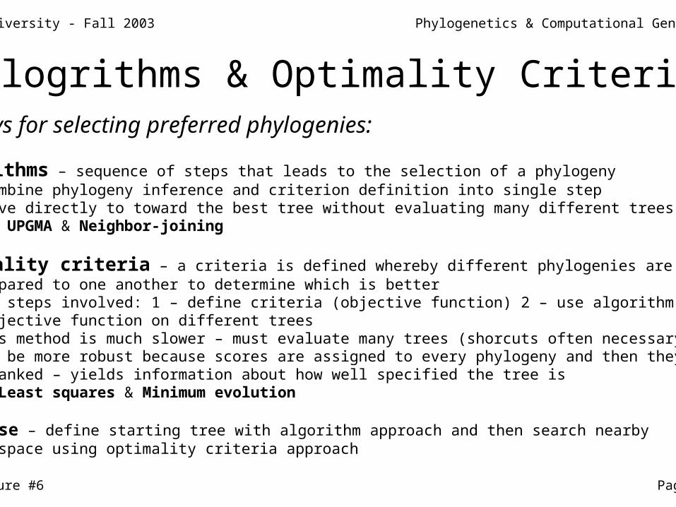
Alogrithms & Optimality CriteriaTwo ways for selecting preferred phylogenies:

Algorithms – sequence of steps that leads to the selection of a phylogeny - combine phylogeny inference and criterion definition into single step - move directly to toward the best tree without evaluating many different trees e.g. UPGMA & Neighbor-joining

Optimality criteria – a criteria is defined whereby different phylogenies are - compared to one another to determine which is better - two steps involved: 1 – define criteria (objective function) 2 – use algorithm to compute objective function on different trees - this method is much slower – must evaluate many trees (shorcuts often necessary) - may be more robust because scores are assigned to every phylogeny and then they are ranked – yields information about how well specified the tree is e.g. Least squares & Minimum evolution

Compromise – define starting tree with algorithm approach and then search nearby tree-space using optimality criteria approach

Lecture #6


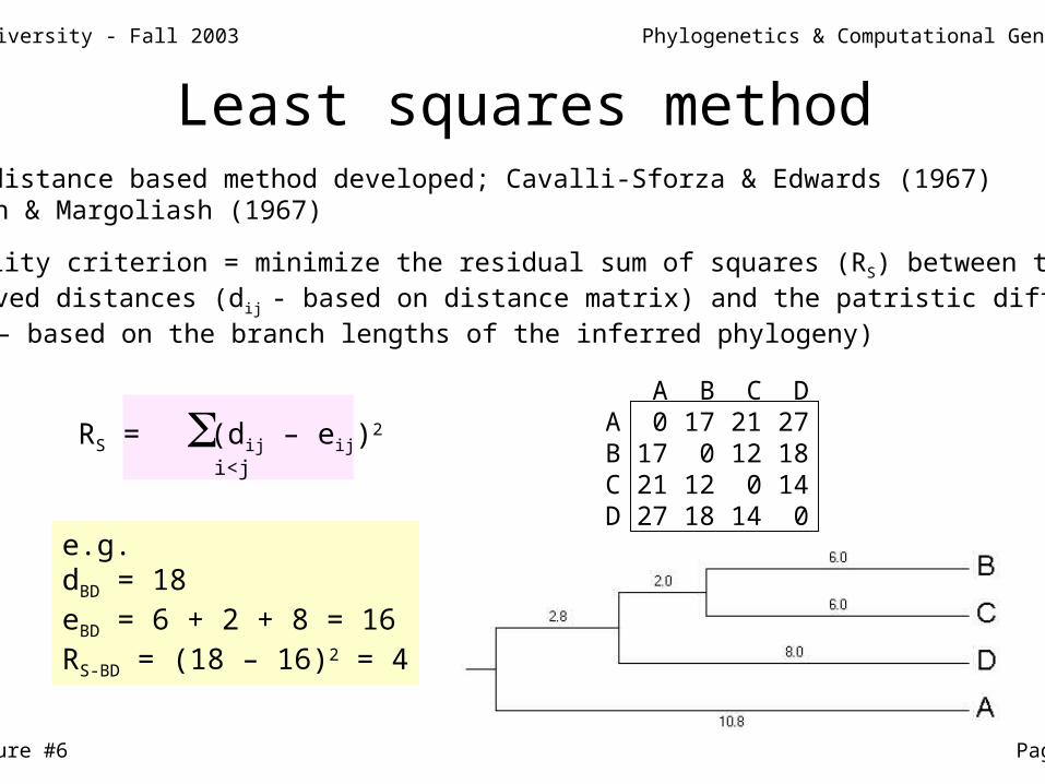
Least squares method First distance based method developed; Cavalli-Sforza & Edwards (1967) Fitch & Margoliash (1967)

Optimality criterion = minimize the residual sum of squares (RS) between the observed distances (dij - based on distance matrix) and the patristic differences (eij – based on the branch lengths of the inferred phylogeny)

RS = (dij – eij)2

i<j

A B C DA 0 17 21 27B 17 0 12 18C 21 12 0 14D 27 18 14 0

e.g.dBD = 18 eBD = 6 + 2 + 8 = 16RS-BD = (18 – 16)2 = 4

Lecture #6


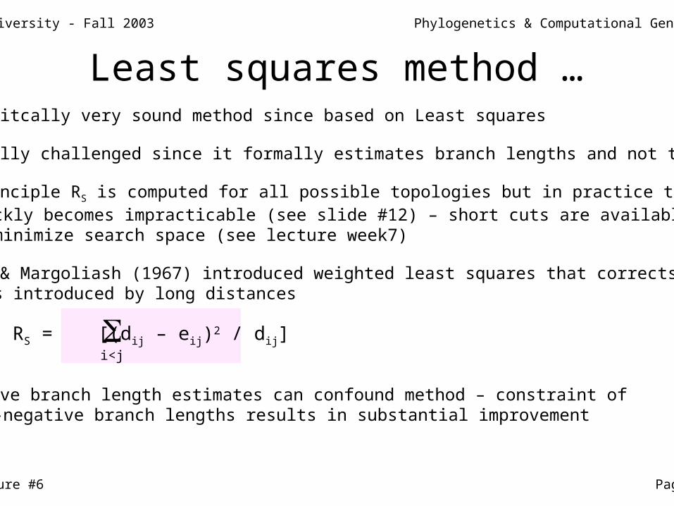
Least squares method … Statisitcally very sound method since based on Least squares

Logically challenged since it formally estimates branch lengths and not topologies

In principle RS is computed for all possible topologies but in practice this quickly becomes impracticable (see slide #12) – short cuts are available to minimize search space (see lecture week7)

Fitch & Margoliash (1967) introduced weighted least squares that corrects for the bias introduced by long distances

Negative branch length estimates can confound method – constraint of non-negative branch lengths results in substantial improvement

RS = [(dij – eij)2 / dij] i<j

Lecture #6


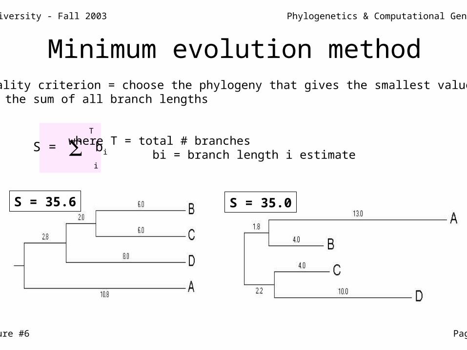
Minimum evolution method Optimality criterion = choose the phylogeny that gives the smallest value of S - the sum of all branch lengths

T

S = bi

i

where T = total # branches bi = branch length i estimate

S = 35.6 S = 35.0

Lecture #6


Minimum evolution method …

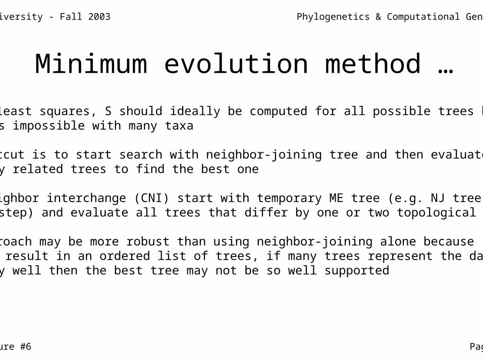
As with least squares, S should ideally be computed for all possible trees but this is impossible with many taxa

One shortcut is to start search with neighbor-joining tree and then evaluate closely related trees to find the best one

Close neighbor interchange (CNI) start with temporary ME tree (e.g. NJ tree for first step) and evaluate all trees that differ by one or two topological changes

This approach may be more robust than using neighbor-joining alone because it can result in an ordered list of trees, if many trees represent the data almost equally well then the best tree may not be so well supported

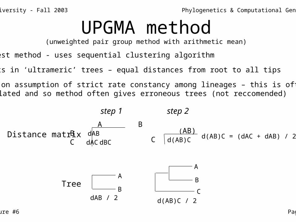
UPGMA method(unweighted pair group method with arithmetic mean)

simplest method - uses sequential clustering algorithm

results in ‘ultrameric’ trees – equal distances from root to all tips

based on assumption of strict rate constancy among lineages – this is often violated and so method often gives erroneous trees (not reccomended)

Lecture #6


A BB dABC dAC dBC

(AB)C d(AB)C d(AB)C = (dAC + dAB) / 2Distance matrix

Tree

dAB / 2

A

B

A

d(AB)C / 2

B

C

step 1 step 2

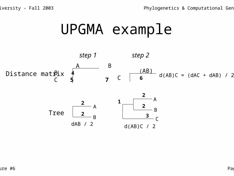
UPGMA example

Lecture #6


A BB 4C 5 7

(AB)C 6 d(AB)C = (dAC + dAB) / 2Distance matrix

Tree

dAB / 2

A

B

A

d(AB)C / 2

B

C

step 1 step 2

2

2

2

21

3

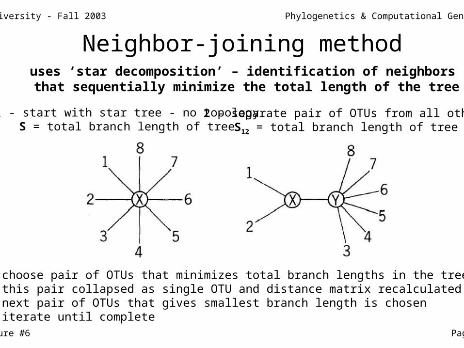
3 - choose pair of OTUs that minimizes total branch lengths in the tree4 - this pair collapsed as single OTU and distance matrix recalculated5 - next pair of OTUs that gives smallest branch length is chosen6 - iterate until complete

1 - start with star tree - no topologyS = total branch length of tree

2 - separate pair of OTUs from all othersS12 = total branch length of tree

uses ‘star decomposition’ – identification of neighbors that sequentially minimize the total length of the tree

Neighbor-joining method

Lecture #6


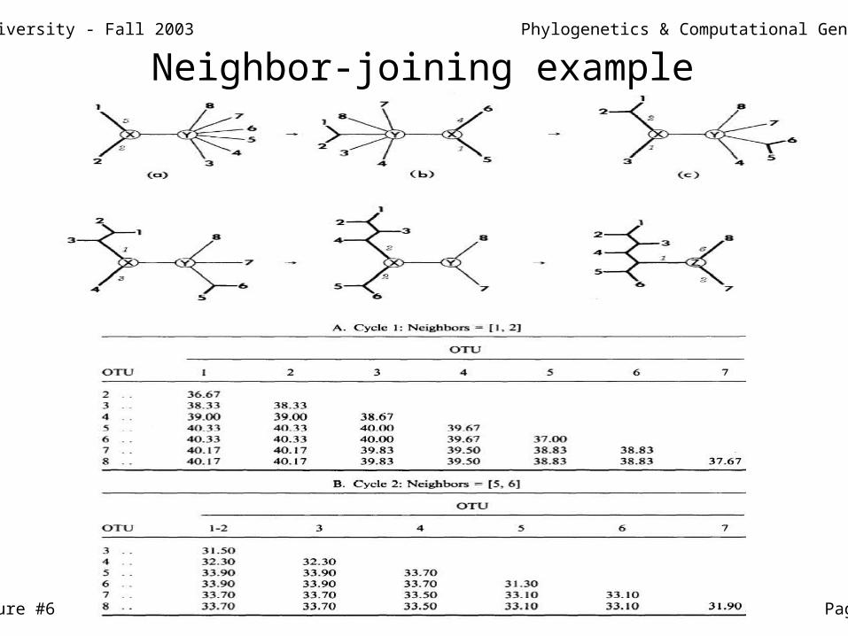
Neighbor-joining example

Lecture #6


Neighbor-joining method …

Lecture #6


Extremely fast and efficient method, widely used & found in numerous publications

Tends to perform fairly well in simulation studies

May produce tie trees from data set but this appears to be rare

Algorithm is ‘greedy’ and so can get stuck in local optima

Main criticism is that it produces only one tree and does not give any idea of how many other trees are equally well or almost as supported by the data

For this reason, neighbor-joining is often used as a method to find a starting tree that other methods (e.g. minimum evolution) will evaluate to find the best tree

Exercises1 - choose some alignment to work on

2 - load alignment into Clustal and build neighbor-joining tree

3 - open tree in Treeview and view, manipulate and save tree

4 - load alignment into DAMBE and into MEGA and reconstruct and view trees using all distance methods available – look for differences in results

5 - manually reconstruct UPGMA tree for the distance matrix on slide #14

6 - open the MEGA formatted version of this same distance matrix http://jhunix.hcf.jhu.edu/~kjordan6/distances.meg in MEGA and reconstruct distance based trees using all 3 methods available (check UPGMA result against manually reconstructed UPGMA tree)

7 - calculate RS for all three distance based trees from #6 and pick best tree

8 - calculate S for all three distance based trees from #6 and pick best tree

Lecture #6


johns hopkins university - fall 2003 phylogenetics & computational genomics - 410.640.71 lecture...

Documents

phylogenetic methods

molecular sequences

phylogenetic tree lecture

powerful methods

primate phylogeny lecture

introduction of distance

development of sequence