joint adaptive colour modelling and skin, hair and clothing segmentation using coherent
TRANSCRIPT
SCHEFFLER AND ODOBEZ: ADAPTIVE COLOUR MODELLING AND SEGMENTATION 1
Joint Adaptive Colour Modelling and
Skin, Hair and Clothing Segmentation
Using Coherent Probabilistic Index Maps
Carl Scheffler
Jean-Marc Odobez
Idiap Research Institute
Centre du Parc
Rue Marconi 19
Martigny, Switzerland
Abstract
We address the joint segmentation of regions around faces into different classes —
skin, hair, clothing and background — and the learning of their respective colour mod-
els. To this end, we adopt a Bayesian framework with two main elements. First, the
modelling and learning of prior beliefs over class colour distributions of different kinds,
viz. discrete distributions for background and clothing, and continuous distributions for
skin and hair. This component of the model allows the formulation of the colour adapta-
tion task as the computation of the posterior beliefs over class colour distributions given
the prior (general) class colour model, a colour likelihood function and observed pixel
colours. Second, a spatial prior based on probabilistic index maps enhanced with Markov
random field regularisation. The inference of the segmentation and of the adapted colour
models is solved using a variational scheme. Segmentation results on a small database
of annotated images demonstrate the impact of the different modelling choices.
1 Introduction
We address the joint segmentation of regions around faces into different classes (skin, hair,
clothing, and background) and the learning of their respective colour models. Such colour in-
formation is known to be a powerful cue for tracking, as has been demonstrated, for instance,
using the mean shift [3] and particle filtering [14] algorithms. In particular, locating skin-
coloured regions plays an important role when dealing with faces, and is useful not only
for face detection and tracking [21, 22], but also for head pose estimation when precisely
segmented and when dealing with low to mid-resolution images. Furthermore, knowing the
colour of a person’s skin, hair and clothing can aid in re-associating lost tracks in video.
Much of the existing literature on skin colour modelling is about building a general
colour model across all possible ethnicities and illumination conditions. Such a model can
still be distracted by objects that are approximately skin-toned, like wood and T-shirts. We
aim to improve skin colour modelling and segmentation by using three main elements. The
first is automatic adaptation of the colour model, either by updating some model parameters
(e.g. of a Gaussian), or by adapting a threshold, or by doing both. The second is to perform
colour segmentation, which brings two main benefits: a form of spatial regularisation and,
c© 2011. The copyright of this document resides with its authors.
It may be distributed unchanged freely in print or electronic forms.

2 SCHEFFLER AND ODOBEZ: ADAPTIVE COLOUR MODELLING AND SEGMENTATION
importantly, the competition between several colour models for class assignment, which re-
solves the issue of setting a threshold for the skin colour model. These two elements —
adaptation and segmentation — are obviously coupled. The main challenge is to obtain ac-
curate colour models, which depends on the choice of good priors for these models and the
selection of appropriate data (pixels) for their estimation or adaptation. The third element
can mitigate this data selection issue. It consists of the exploitation of a spatial prior on the
location of each class label. The intuition is that knowing the approximate location of, for
instance, a person’s hair and clothing provides a lot of information about where his/her face
is located (and vice versa). A spatial prior also helps to avoid drift, explicitly for segmen-
tation and implicitly for colour adaptation. In this paper, we combine the three elements
above within a generative model of face images. More precisely, the main components and
novelties of our model are as follows.
• The colour model of each class (skin, hair, clothing and background) is represented
with a probability distribution over colours, which we will refer to as a palette. For
each class, we learn a prior distribution over palettes — i.e., a distribution over colour
distributions — across all people. This contrasts with the literature where a prior
model is an expected colour distribution across all people. The parameters of this
prior can then be updated online, to do adaptation. Furthermore, we use different
types of colour models for different classes — continuous models for skin and hair,
and discrete models for background and clothing.
• We use a spatial prior over classes based on probabilistic index maps (PIMs) [6].
The standard PIM model is modified by incorporating a Markov random field prior
to model correlations between neighbouring pixels.
• Inference in the full Bayesian model is done using a variational approach that com-
putes approximate Bayesian posteriors over the class of each image pixel for segmen-
tation and over the palette of each class for colour adaptation.
The impact and validity of the different components are evaluated on a small dataset.
The remainder of the paper is organised as follows. Section 2 discusses related work
on skin and hair colour modelling. The proposed Bayesian model is described in Section 3.
The data set used for training and testing is presented in Section 4. The different inference
procedures are summarised in Section 5, while Section 6 shows the experimental results.
The supplementary material accompanying this article contains derivations of the inference
procedure described here, along with additional qualitative results. Source code and data for
reproducing the results described here is available from [1].
2 Related Work
Here we briefly review the skin colour modelling literature, focusing on adaptive models,
which are more relevant to the scope of this paper. We also briefly review the more recent
work on hair segmentation.
Skin Modelling There is a strong body of literature on general skin colour modelling, but
less so for adaptation of a colour model to an individual person. Kakumanu et al. [10]
provide a recent and comprehensive survey of the field. They provide overviews of colour
spaces, parametric and non-parametric models for colour distributions, public databases, il-
lumination invariance and adaptation. However, they make no mention of adapting a general

SCHEFFLER AND ODOBEZ: ADAPTIVE COLOUR MODELLING AND SEGMENTATION 3
skin colour model to an individual person.
One of the strongest colour models for classifying pixels into skin and background with-
out adaptation is the histogram-based model of Jones and Rehg [7]. They provide a large
labelled database of skin and background images, known as the Compaq skin database, and
estimate the probability of observing each of the 2563 possible RGB triples in skin and non-
skin pixels. They then use Bayes’ rule and the likelihood ratio between the two models to
compute the probability that a given pixel is skin or not, thus avoiding having to set a skin
likelihood threshold. When comparing colour spaces, Phung et al. [15] conclude that 2563
histogram bins should be used for the general skin model (assuming that there are enough
training images) in any 3-d colour space, but not in a reduced colour space, such as a 2-d
chroma-only space. Luminance is important, as also pointed out by Kakumanu et al. [10].
Skin Adaptation Adaptation to illumination changes has been studied for both video and
single images. However, the underlying assumptions are often different from the scope of
this article — the focus is more on large and possibly abrupt illumination changes with
respect to direction, intensity and colour, e.g. [16].
Adaptation of a general skin colour model to an individual person has mainly been con-
sidered in the context of face tracking. In the large majority of cases (e.g., [11, 12, 17, 19,
21, 22]), colour adaptation is presented as first learning a general colour model in the form
of a Gaussian, Gaussian mixture or histogram, and then re-estimating the model parameters
using selected data from a new image. Surprisingly, the use of a proper Bayesian approach
as proposed here has not been considered. A typical example of the approach described
above is in [21]. A single 2-d Gaussian is used for a general colour distribution, defined in
an intensity normalised red–green colour space. The sample mean and covariance of pixels
classified as skin in a new frame are used to adapt the mean and covariance of the Gaussian
skin model using auto-regressive temporal smoothing.
The decision about which pixels to use for updating the skin model relies on two types of
constraints, viz. chromatic and geometric. Soriano et al. [17] argue for the use of chromatic
constraints rather than geometric constraints, and thus follow the approach of [21] sum-
marised above, except that a skin histogram model is used. However, chromatic constraints
can easily fail, either due to the lack of data for adaptation when the colour discrepancy with
the general colour model is too great, or due to model drift in the presence of nearby skin-
coloured hair, background or clothing regions. Geometric constraints have been used in a
weak fashion for data selection — e.g., by sampling the most reliable skin pixel locations
given a face bounding box as provided by a tracker or a face detector [12, 22] — and to
select background pixels when adapting a background colour model in order to apply a (de-
sirable) colour likelihood ratio test rather than using a fixed threshold. However, in the latter
case blond or red hair can often be confused with skin, since this reliability-driven geometric
constraint will avoid selecting background pixels near the face.
In this work, we use both chromatic and geometric constraints in a principled Bayesian
framework for colour distribution adaptation.
Hair Colour Segmentation More recently, a few papers have addressed the problem of
hair segmentation [9, 11, 19, 20]. Most of these use similar approaches to the skin detection
literature, but usually also exploit a segmentation algorithm, e.g. a graph-cut method in [11]
and a snake-based active contour in [9]. Although they are computationally efficient, these
methods do not have the same properties as our approach. Some use a simple colour model
or geometric prior that allow them to work with a controlled background, or assume little
variation in hair styles or pose, and they all lack a probabilistic framework for adaptation.
4 SCHEFFLER AND ODOBEZ: ADAPTIVE COLOUR MODELLING AND SEGMENTATION
k ∈ classes
x,y
I
CPIM
Col
⟨
zIxy
⟩
~ΘIk
~cIxy
I
k ∈ {discrete classes}
x,y
~α(c)k
D(
~π(c)Ik
∣
∣~α(c)k
)
~π(c)Ik
[~π(c)I,zIxy
]bin(~cIxy)
vbin
~cIxy
zIxy
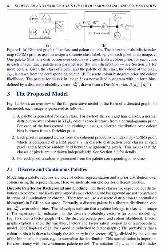
(a) (b)Figure 1: (a) Directed graph of the class and colour models. The coherent probabilistic index
map (CPIM) prior is used to assign a discrete class label, zIxy, to each pixel in an image, I.
One palette (that is, a distribution over colours) is drawn from a colour prior, for each class
in each image. Each palette is a parametrised (by ΘIk) distribution — see Section 3.1 for
more details. Given the class of a pixel and the palette of the class, the colour of the pixel,
~cIxy, is drawn from the corresponding palette. (b) Discrete colour histogram prior and colour
likelihood. The palette for class k in image I is a normalised histogram with uniform bins,
defined by a discrete probability vector, ~π(c)Ik , drawn from a Dirichlet prior, D
(
~π(c)Ik
∣
∣~α(c)k
)
.
3 The Proposed Model
Fig. 1a shows an overview of the full generative model in the form of a directed graph. In
the model, each image is generated as follows:
1. A palette is generated for each class. For each of the skin and hair classes, a normal
distribution over colours in YPbPr colour space is drawn from a normal–gamma prior.
For each of the background and clothing classes, a discrete distribution over colour
bins is drawn from a Dirichlet prior.
2. Each pixel is assigned a class from the coherent probabilistic index map (CPIM) prior,
which is comprised of a PIM prior (i.e., a discrete distribution over classes at each
pixel) and a Markov random field between neighbouring pixels. This means that the
classes of pixels are not drawn independently. See Section 3.2 for details.
3. For each pixel, a colour is generated from the palette corresponding to its class.
3.1 Discrete and Continuous Palettes
Modelling a palette requires a choice of colour representation and a prior distribution over
colours using the representation. Here we motivate our choices for different palettes.
Discrete Palettes for Background and Clothing For these classes we expect colour distri-
butions to be broad and likely multi-modal since clothing and background are not constrained
in terms of illumination or chroma. Therefore we use a discrete distribution (a normalised
histogram) in RGB colour space. Formally, a discrete palette is a discrete distribution vec-
tor, ~π(c)Ik , over colour bins. The subscripts indicate that a palette belongs to class k in image
I. The superscript (c) indicates that this discrete probability vector is for colour modelling.
Fig. 1b shows a factor graph [4] of the discrete palette prior and colour likelihood. (Factor
graphs explicitly show the variables, factors and factorisation properties of a probabilistic
model. See Chapter 8 of [2] for a good introduction to factor graphs.) The probability that a
colour in bin b is drawn is simply the bth entry in the vector, [~π(c)Ik ]b, divided by the volume
of the bin in colour space, vbin, to normalise the distribution. This normalisation is important
for consistency with the continuous palette model. The notation [~a]b ≡ ab is used to index

SCHEFFLER AND ODOBEZ: ADAPTIVE COLOUR MODELLING AND SEGMENTATION 5
I
k ∈ continuous classes
x,y
~η(c)k
~τ(c)k
~α(c)k
~β(c)k
NG(
~µ(c)Ik ,~λ
(c)Ik
∣
∣~η(c)k ,~τ
(c)k ,~α
(c)k ,~β
(c)k
)
~µ(c)Ik
~λ(c)Ik
N(
~cIxy
∣
∣~µ(c)I,zIxy
,(~λ(c)I,zIxy
)−1)
~cIxy
zIxy
Figure 2: Continuous colour model and likelihood. The palette for class k in image I is
a product of normal distributions over the three colour components — Y, Pb and Pr —
parametrised by means, ~µ(c)Ik , and precisions (inverse variances), ~λ
(c)Ik . Each mean and in-
verse variance is drawn from a normal–gamma (NG) prior.
into a vector. The square brackets simply serve to aid legibility. The prior distribution over
palettes, which can also be interpreted as the general distribution over colours for the class,
is chosen to be the Dirichlet distribution, which is conjugate to the discrete distribution.
Continuous Palettes for Skin and Hair We model each of the skin and hair palettes using
an axis-aligned normal distribution in YPbPr colour space. This space is used in the JPEG
compression standard and was designed to separate lightness from colour. As reported in the
literature, skin tone as represented by the chroma components (Pb and Pr) is very localised
for skin in general [17] and we expect it to be even more localised for the skin of an individual
person. Fig. 2 shows a factor graph of the continuous palette prior and colour likelihood. A
continuous palette is a factored normal distribution over colour components, parametrised
by a mean vector, ~µ(c)k , and a precision vector,~λ
(c)k . We use the conjugate normal–gamma
distribution as palette prior. The conjugacy makes for straightforward analytical inference
and computationally efficient update equations — see Section 5 for details.
We would like to emphasise that, to the best of our knowledge, modelling general skin
colour as a distribution over distributions has not been explored in the literature, where both
the general and adapted skin colour models are usually handled as distributions over colours.
The advantage of our approach is that estimating the adapted colour model is handled in a
principled Bayesian framework by estimating the posterior belief over, for example, a per-
son’s skin palette based on the prior (general) skin model and the colour likelihood function.
3.2 Coherent Probabilistic Index Maps (CPIM)
In this section, we first describe the probabilistic index map (PIM) of Jojic and Caspi [6],
and then our extension using a Markov random field.
Probabilistic Index Maps The main objective of the PIM model is to learn a prior over the
class of each pixel in an image. The idea is that the segmentation maps of (aligned) images
of the same object are often consistent across instances, even if the pixels of the same class
across training images are not characterised by the same colour distribution parameters —
i.e., they have different palettes. More formally, the PIM prior is defined as:
PPIM
(⟨
zxy
⟩ ∣
∣
⟨
~π(z)xy
⟩)
= ∏x,y
[
~π(z)xy
]
zxy(1)
where⟨
zxy
⟩
denotes the set of class label variables at all pixel coordinates, and ~π(z)xy is a dis-
crete probability vector over classes at pixel (x,y). The PIM model assumes an independent

6 SCHEFFLER AND ODOBEZ: ADAPTIVE COLOUR MODELLING AND SEGMENTATION
x,y
I
~π(z)xy
[~π(z)xy ]zIxy
zIxy
x,y
I
~π(z)xy
[~π(z)xy ]zIxy
zIxy
e−EMRF(〈zIxy〉)
kMRF
(a) (b)
Figure 3: (a) The PIM model. The distribution over classes at each (x,y) coordinate is inde-
pendent of the other coordinates. The class zIxy is drawn from a discrete latent distribution
~π(z)xy . (b) CPIM: the coherent PIM model. The distribution over classes at each (x,y) coordi-
nate depends on its four neighbours through a Markov random field.
prior over pixels, and hence spatial consistency is not incorporated. The prior parameters,⟨
~π(z)xy
⟩
, are estimated from images with ground truth class labels for each pixel.
Incorporating a Markov Random Field We know that adjacent pixels in an image belong
to the same class with high probability. This knowledge is encoded in the prior over classes
by incorporating into the PIM model a coherence energy function in the form of a Markov
random field that encourages neighbouring pixels to be in the same class. The standard PIM
prior (1) is modified as follows:
PMRF
(⟨
zxy
⟩∣
∣
⟨
~π(z)xy
⟩
,kMRF
)
∝ PPIM
(⟨
zxy
⟩∣
∣
⟨
~π(z)xy
⟩)
e−EMRF(〈zxy〉) (2)
where the Markov random field (MRF) energy function is
EMRF
(⟨
zxy
⟩)
=−kMRF ∑(xy,uv)∈C
I [zxy = zuv] (3)
and C denotes the set of pairwise cliques (i.e. the set of pairs of neighbouring coordinates
(x,y) and (u,v) — we use a 4-connected neighbouring system) in the image and kMRF is
a constant indicating how important it is that adjacent pixels have the same class. This
modified prior will be referred to as coherent PIM (CPIM). The factor graphs for PIM and
coherent PIM are shown in Fig. 3.
4 Data
We used the Compaq skin database [7] for all of the training and evaluation in this article.
The full database contains more than 13,000 images in two groups — skin and non-skin.
Skin images have ground truth indicating which pixels contain skin, but this labelling was
done conservatively in the sense that labels have very high precision (presumably 100%) but
low recall. Therefore we can use the labels to construct a good skin colour model, but not
to test the accuracy of skin segmentation. Non-skin images in the database were used to
learn the background colour model prior, as described in the next section. The background
prior was also used as the prior for clothing, since we expect that clothing can be any colour
and since there is not enough labelled data to estimate a good prior for clothing. To learn
the CPIM prior maps (and for testing), several images from the database containing faces
detected by the Viola–Jones face algorithm [18] as implemented in the OpenCV library [5]
were labelled for skin, hair, clothing and background. The size of a cropped image was
chosen to be twice the size of the bounding box returned by the face detector, yielding a set
of head-and-shoulder images, as illustrated in Fig. 4a.

SCHEFFLER AND ODOBEZ: ADAPTIVE COLOUR MODELLING AND SEGMENTATION 7
(a) (b) (c) (d) (e)
Figure 4: (a) Example of an annotated image with skin (yellow), hair (red), clothing (green)
and background (blue). White regions are unlabelled and usually close to boundaries where
it is difficult to discriminate between classes. Unlabelled pixels were not used for training or
testing. (b)–(e) The PIM prior that each pixel belongs to the skin, hair, clothing and back-
ground classes, respectively. Black indicates high probability and white, low probability.
5 Inference
Inference is done in two stages. Firstly, the prior parameters for CPIM and for each of
the colour palettes are estimated from training data. Secondly, using these priors and given
a test image, approximate Bayesian posterior beliefs over the class of each pixel and the
colour distribution for each class are computed. The inference procedures for these stages
are summarised below, with mathematical derivations, which are straightforward but lengthy,
relegated to the supplementary material.
PIM Prior The PIM prior parameters,⟨
~π(z)xy
⟩
, are estimated directly from the fully labelled
images by counting the number of times that each pixel belongs to each class in the train-
ing data. Left–right symmetry is enforced by flipping and averaging the estimated priors.
Fig. 4b–e shows the resulting distribution over classes at each pixel in the image.
Discrete Palette Prior The Dirichlet prior for the discrete background palette (see Fig. 1b)
is learned from all pixels in the non-skin images of the Compaq database. The discrete
distribution for each image, ~π(c)Ik , can be integrated out analytically to get a Pólya distribution
over the number of times that the colours in each histogram bin appear in each image. We
estimate a regularised maximum likelihood setting of ~α(c)k for this distribution using the
method of Minka [13]. The regularisation simply adds a small initial count to each histogram
bin so as to avoid numerical singularities associated with zero counts. The mean of the
Dirichlet prior over the background palette is visualised in Fig. 5a.
Due to a lack of labelled training data for clothing pixels, the prior distribution estimated
for the background palette is also used as the prior for the clothing palette.
Continuous Palette Prior The prior parameters for continuous colour distributions are also
estimated using a regularised maximum likelihood procedure. In this case the data likelihood
is a bit more complex than for discrete distributions. First, we compute the maximum like-
lihood estimate for the normal distribution over colours in each image in the training data.
Next, the maximum likelihood fit of the palette prior parameters is computed by numeri-
cal optimisation. The prior parameters (~η , ~τ , ~α and ~β ) were introduced in Fig. 2. Each
parameter vector has 3 entries for the 3 colour components. Since colour distributions are
axis-aligned, we optimise one entry from each of these vectors (i.e., 4 parameters) at a time.
The skin palette prior is estimated from the skin pixels in the face region of each Compaq
image in which a face was detected. The hair palette prior is estimated from the much smaller
set of fully labelled images from the same database. The marginals over colours from the
8 SCHEFFLER AND ODOBEZ: ADAPTIVE COLOUR MODELLING AND SEGMENTATION
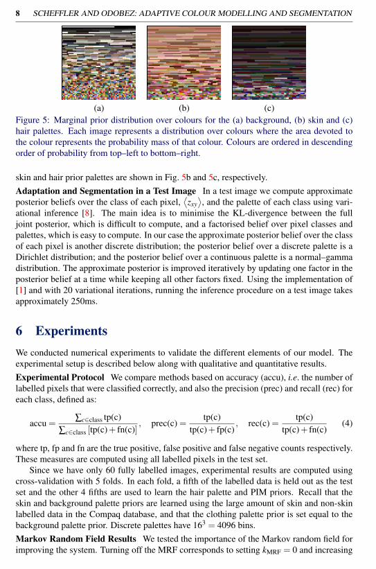
(a) (b) (c)
Figure 5: Marginal prior distribution over colours for the (a) background, (b) skin and (c)
hair palettes. Each image represents a distribution over colours where the area devoted to
the colour represents the probability mass of that colour. Colours are ordered in descending
order of probability from top–left to bottom–right.
skin and hair prior palettes are shown in Fig. 5b and 5c, respectively.
Adaptation and Segmentation in a Test Image In a test image we compute approximate
posterior beliefs over the class of each pixel,⟨
zxy
⟩
, and the palette of each class using vari-
ational inference [8]. The main idea is to minimise the KL-divergence between the full
joint posterior, which is difficult to compute, and a factorised belief over pixel classes and
palettes, which is easy to compute. In our case the approximate posterior belief over the class
of each pixel is another discrete distribution; the posterior belief over a discrete palette is a
Dirichlet distribution; and the posterior belief over a continuous palette is a normal–gamma
distribution. The approximate posterior is improved iteratively by updating one factor in the
posterior belief at a time while keeping all other factors fixed. Using the implementation of
[1] and with 20 variational iterations, running the inference procedure on a test image takes
approximately 250ms.
6 Experiments
We conducted numerical experiments to validate the different elements of our model. The
experimental setup is described below along with qualitative and quantitative results.
Experimental Protocol We compare methods based on accuracy (accu), i.e. the number of
labelled pixels that were classified correctly, and also the precision (prec) and recall (rec) for
each class, defined as:
accu =∑c∈class tp(c)
∑c∈class [tp(c)+ fn(c)], prec(c) =
tp(c)
tp(c)+ fp(c), rec(c) =
tp(c)
tp(c)+ fn(c)(4)
where tp, fp and fn are the true positive, false positive and false negative counts respectively.
These measures are computed using all labelled pixels in the test set.
Since we have only 60 fully labelled images, experimental results are computed using
cross-validation with 5 folds. In each fold, a fifth of the labelled data is held out as the test
set and the other 4 fifths are used to learn the hair palette and PIM priors. Recall that the
skin and background palette priors are learned using the large amount of skin and non-skin
labelled data in the Compaq database, and that the clothing palette prior is set equal to the
background palette prior. Discrete palettes have 163 = 4096 bins.
Markov Random Field Results We tested the importance of the Markov random field for
improving the system. Turning off the MRF corresponds to setting kMRF = 0 and increasing

SCHEFFLER AND ODOBEZ: ADAPTIVE COLOUR MODELLING AND SEGMENTATION 9
0 1 2 3 4 5 60.80
0.81
0.82
0.83
0.84
0.85
disc
cont
class s (con) h (con) c (dis) b (dis)
precision 0.951 0.820 0.725 0.853
recall 0.846 0.626 0.869 0.922
class s (dis) h (dis) c (dis) b (dis)
precision 0.919 0.780 0.746 0.876
recall 0.882 0.677 0.849 0.896
(a) (b)
Figure 6: Markov random field experiments. (a) Overall accuracy as a function of the field
strength, kMRF. Blue circles show the results when using continuous skin and hair palettes,
and red triangles when using discrete palettes. (b) Precision and recall values at kMRF = 3 for
each class (skin, hair, clothing, background) under both conditions (continuous and discrete).
this constant corresponds to strengthening the MRF, meaning that neighbouring pixels are
more likely to belong to the same class. Fig. 6 summarises the results of the experiment.
The accuracy jumps by about 4% when the Markov random field is turned on (kMRF = 1),
but then saturates quickly for larger values of the field strength. The maximum was found to
be at kMRF = 3. This shows that the MRF is an important part of the model.
Continuous vs Discrete Palettes To test the value of using continuous palettes, we also ran
the above experiment with discrete palettes for the skin and hair classes, keeping the other
experimental conditions the same as before. In this case the predictive accuracy is about the
same, but the same dependence on the presence of the MRF is observed, as shown in Fig. 6a.
The main difference lies in the precision and recall for each type of colour distribution. Note
from Fig. 6b that recall for skin classification improves when using the discrete palette, but at
the cost of precision. It appears that since the discrete palette is a more flexible representation
than the continuous one, it adapts to cover more skin-coloured pixels, but that same flexibility
also causes it to cover non-skin pixels. One should prefer one model type over the other based
on the application of the overall model.
7 Conclusion
This paper addressed the joint segmentation and colour adaptation task. Our contributions
are: a Bayesian method for computing and adapting hyper-beliefs over skin palettes (i.e.,
distributions over distributions rather than expected distributions), the mixing of discrete and
continuous palettes, the combination of a Markov random field prior with the probabilistic
index map model, and a variational inference procedure. Numerical results demonstrated
the validity of the approach. Future work includes the use of this model for head pose
estimation and tracking. One limitation of our approach is the single spatial prior, which
could be improved by considering mixture models, e.g. of different hair styles [11].
This work was supported by the European Community’s Seventh Framework Program (FP7/2007-2013) un-
der the TA2 project (Together Anywhere, Together Anytime), grant agreement no. ICT-2007-214793, and the
HUMAVIPS project (Humanoids with Auditory and Visual Abilities in Populated Spaces), grant agreement no.
ICT-2009.2.1-247525.

10 SCHEFFLER AND ODOBEZ: ADAPTIVE COLOUR MODELLING AND SEGMENTATION
(a) (b) (c) (d)Figure 7: Results of segmenting two challenging images into skin (yellow), hair (red), cloth-
ing (green), and background (blue) regions. Pixels for which the class posterior probability
was below 95% were left white. (a) Original image. (b) Segmentation with full model, using
continuous skin and hair palettes. (c) Segmentation without the MRF. (d) Segmentation us-
ing discrete palettes. In the first image both the background and the face are skin-coloured,
but the model is able to separate them well. In the second image the person has no hair and
the shadow in the background forms a region that can be interpreted as hair. This fools the
method into fitting the hair palette to this region.
References
[1] Adaptive face colour modelling and segmentation project page. URL http://www.
idiap.ch/software/facecolormodel/.
[2] C. M. Bishop. Pattern Recognition and Machine Learning. Springer, 2006.
[3] D. Comaniciu and P. Meer. Mean shift: a robust approach toward feature space analy-
sis. IEEE Transactions on Pattern Analysis and Machine Intelligence, 24(5):603–619,
2002.
[4] B. J. Frey. Graphical Models for Machine Learning and Digital Communication. MIT
Press, 1998.
[5] Intel Corporation. OpenCV, version 2.0.0, October 2009. URL http://opencv.
willowgarage.com/wiki/.
[6] N. Jojic and Y. Caspi. Capturing image structure with probabilistic index maps. In
IEEE Conference on Computer Vision and Pattern Recognition, 2004.
[7] M. J. Jones and J. M. Rehg. Statistical color models with application to skin detection.
International Journal of Computer Vision, 46:81–96, 2002.
[8] M. I. Jordan, Z. Ghahramani, T. S. Jaakkola, and L. K. Saul. An introduction to varia-
tional methods for graphical models. Machine Learning, 37:183–233, 1999.
[9] P. Julian, C. Dehais, F. Lauze, V. Charvillat, A. Bartoli, and A. Choukroun. Automatic
hair detection in the wild. In International Conference on Pattern Recognition, 2010.
[10] P. Kakumanu, S. Makrogiannis, and N. Bourbakis. A survey of skin-color modeling
and detection methods. Pattern Recognition, 40(3):1106–1122, 2007.

SCHEFFLER AND ODOBEZ: ADAPTIVE COLOUR MODELLING AND SEGMENTATION 11
[11] K. Lee, D. Anguelov, B. Sumengen, and S. B. Gokturk. Markov random field models
for hair and face segmentation. In Automatic Face and Gesture Recognition, 2008.
[12] C. Liensberger, J. Stottinger, and M. Kampel. Color-based and context-aware skin
detection for online video annotation. In IEEE International Workshop on Multimedia
Signal Processing, 2009.
[13] T. Minka. Estimating a Dirichlet distribution. Technical report, 2009.
[14] P. Perez, C. Hue, J. Vermaak, and M. Gangnet. Color based probabilistic tracking. In
European Conference on Computer Vision, 2002.
[15] S. L. Phung, A. Bouzerdoum, and D. Chai. Skin segmentation using color pixel classifi-
cation: Analysis and comparison. IEEE Transactions on Pattern Analysis and Machine
Intelligence, 27(1):148–154, 2005.
[16] L. Sigal, S. Sclaroff, and V. Athitsos. Skin color-based video segmentation under time-
varying illumination. IEEE Transactions on Pattern Analysis and Machine Intelligence,
26(7):862–877, 2004.
[17] M. Soriano, B. Martinkauppi, S. Huovinen, and M. Laaksonen. Adaptive skin color
modeling using the skin locus for selecting training pixels. Pattern Recognition, 36:
681–690, 2003.
[18] P. Viola and M. Jones. Robust real-time face detection. International Journal of Com-
puter Vision, 57(2):137–154, 2004.
[19] D. Wang, X. Chai, H. Zhang, H. Chang, W. Zeng, and S. Shan. A novel coarse-to-fine
hair segmentation method. In Automatic Face and Gesture Recognition, 2011.
[20] Y. Yacoob and L. S. Davis. Detection and analysis of hair. IEEE Transactions on
Pattern Analysis and Machine Intelligence, 28(7), 2006.
[21] J. Yang and A. Waibel. A real-time face tracker. In IEEE Workshop on Applications of
Computer Vision, pages 142–147, 1996.
[22] T. Yoo and I. Oh. A fast algorithm for tracking human faces based on chromatic his-
tograms. Pattern Recognition Letters, 20:967–978, 1999.
SCHEFFLER AND ODOBEZ: ADAPTIVE COLOUR MODELLING AND SEGMENTATION 1
Joint Adaptive Colour Modelling and
Skin, Hair and Clothing Segmentation
Using Coherent Probabilistic Index Maps
Supplementary Material
Carl Scheffler
Jean-Marc Odobez
Idiap Research Institute
Centre du Parc
Rue Marconi 19
Martigny, Switzerland
Contents
1 Introduction 2
2 Variational Inference 2
2.1 Full Generative Model . . . . . . . . . . . . . . . . . . . . . . . . . . . . 2
2.2 Approximating Distribution . . . . . . . . . . . . . . . . . . . . . . . . . . 4
2.3 Variational Update Equations . . . . . . . . . . . . . . . . . . . . . . . . . 5
2.3.1 Update for Class Variables . . . . . . . . . . . . . . . . . . . . . . 5
2.3.2 Update for Discrete Palettes . . . . . . . . . . . . . . . . . . . . . 6
2.3.3 Update for Continuous Palettes . . . . . . . . . . . . . . . . . . . 7
2.3.4 Summary . . . . . . . . . . . . . . . . . . . . . . . . . . . . . . . 8
3 Setting the Prior Parameters 8
3.1 Class Variables . . . . . . . . . . . . . . . . . . . . . . . . . . . . . . . . 8
3.2 Discrete Palettes . . . . . . . . . . . . . . . . . . . . . . . . . . . . . . . . 8
3.3 Continuous Palettes . . . . . . . . . . . . . . . . . . . . . . . . . . . . . . 9
4 More Experimental Results 9
5 Probability Distributions 14
6 Colour Spaces 14
6.1 RGB . . . . . . . . . . . . . . . . . . . . . . . . . . . . . . . . . . . . . . 14
6.2 YCbCr / YPbPr . . . . . . . . . . . . . . . . . . . . . . . . . . . . . . . . 14
This work was supported by the European Community’s Seventh Framework Program (FP7/2007–
2013) under the TA2 project (Together Anywhere, Together Anytime), grant agreement no. ICT–2007–
214793, and the HUMAVIPS project (Humanoids with Auditory and Visual Abilities in Populated
Spaces), grant agreement no. ICT–2009.2.1–247525.
c© 2011. The copyright of this document resides with its authors.
It may be distributed unchanged freely in print or electronic forms.
2 SCHEFFLER AND ODOBEZ: ADAPTIVE COLOUR MODELLING AND SEGMENTATION
1 Introduction
This document contains the supplementary material for the main conference article by the
same title. The main purposes of this material are to show the derivations of key equations
for probabilistic inference and to present more qualitative experimental results. Note that this
document is not self-contained in that it references the main article in a number of places.
2 Variational Inference
Variational inference [5] is an approximate Bayesian inference scheme. The main idea is to
minimise the Kullback–Leibler divergence between the full joint distribution over all latent
variables in a model (which is difficult to compute) and an approximating distribution over
the model variables (which is easy to compute). The approximating distribution usually
factorises at least partially in the variables of the model. In this case it can be shown that
updating (optimising) each factor while keeping the other factors fixed strictly improves an
upper bound on the divergence between the true and approximating distributions.
In this section we derive the update equations used to infer posterior beliefs over the class
of each pixel in an image, and over the discrete and continuous palettes associated with each
class in an image.
2.1 Full Generative Model
In an image, I, each pixel belongs to a discrete class, zIxy, which determines the colour
model used to generate the colour of the pixel, ~cxy. The classes are skin, hair, clothing and
background. The x and y subscripts are the coordinates of the pixel. The class of a pixel is
generated from a discrete distribution with parameters ~π(z)xy .
There is also a Markov random field (MRF) dependence between neighbouring class
pixels. The neighbours of a pixel are the 4 pixels to the north, south, east and west of it. A
pixel is conditionally independent of all other pixels given its neighbours.
The model described above is referred to as a coherent probabilistic index map (CPIM) in
the main article. According to the CPIM model, the class labels in each image are generated
according to
PCPIM
(
⟨
zIxy
⟩
∣
∣
∣
⟨
~π(z)xy
⟩
,kMRF
)
=
[
∏x,y
[
~π(z)xy
]
zIxy
]
exp
(
kMRF ∑(xy,uv)∈C
I [zIxy = zIuv]
)
(1)
C denotes the set of pairwise cliques — i.e. the set of neighbours. The square bracket
notation [~π]a is used to refer to the value in vector ~π at index a. This is equivalent to writing
πa; the square bracket notation is used to aid legibility.
SCHEFFLER AND ODOBEZ: ADAPTIVE COLOUR MODELLING AND SEGMENTATION 3
There are two types of palettes (colour models), viz. discrete and continuous. Each dis-
crete palette is represented by a discrete probability vector, ~π(c)Ik , and is generated from a
Dirichlet prior with parameter ~αk. The discrete palette for class k in image I is generated
according to
Ppal:disc
(
~π(c)Ik
∣
∣
∣
~α(c)k
)
= Dirichlet(
~π(c)Ik
∣
∣
∣
~α(c)k
)
(2)
For a pixel at coordinates (x,y) that belongs to class zIxy = k, its colour, ~cIxy, is drawn
from the discrete probability vector ~π(c)Ik .
Pcol:disc
(
~cIxy
∣
∣
∣
~π(c)Ik
)
= v−1bin
[
~π(c)Ik
]
bin(~cIxy)(3)
Here bin(·) is the function that maps a colour vector to its bin in the colour histogram and
vbin is the volume of each bin in colour space. Dividing by the volume ensures that the distri-
bution over colour vectors is normalised. Each colour vector is a RGB triple (see Section 6
for details on colour spaces). The colour space is discretised into uniformly distributed cubes
in RGB space. In this work 16 bins are used per colour dimension, for a total of 163 = 4096
bins.
Each continuous palette is represented by a normal distribution over colour components
in YPbPr colour space (see Section 6). This 3-dimensional normal distribution has inde-
pendent components, where each component is parametrised by its mean, µ j, and precision
(inverse variance), λ j. The continuous palette for class k in image I is generated according
to
Ppal:cont
(
~µ(c)Ik ,~λ
(c)Ik
∣
∣
∣
~η(c)k ,~τ
(c)k ,~α
(c)k ,~β
(c)k
)
=3
∏j=1
Normal(
µ(c)Ik j
∣
∣
∣η(c)k j ,(τ
(c)k j λ
(c)Ik j )
−1)
Gamma(
λ(c)Ik j
∣
∣
∣α(c)k j ,β
(c)k j
)
(4)
where the gamma distribution is parametrised by its shape, α , and inverse length scale, β .1
For a pixel at coordinates (x,y) that belongs to class zIxy = k, its colour, ~cIxy, is drawn
from the normal distribution defined by ~µ(c)Ik and~λ
(c)Ik .
Pcol:cont
(
~cIxy
∣
∣
∣
~µ(c)Ik ,~λ
(c)Ik
)
=3
∏j=1
Normal(
cIxy j
∣
∣
∣µ(c)Ik j ,(λ
(c)Ik j )
−1)
(5)
where~cIxy is a vector in YPbPr colour space.
1Note that the gamma distribution is often parametrised by shape, k = α , and length scale, θ = β−1, parameters
instead.
4 SCHEFFLER AND ODOBEZ: ADAPTIVE COLOUR MODELLING AND SEGMENTATION
Given equations (1)–(5), the full generative model for a set of images is
∏I∈images
[
PCPIM
(
⟨
zIxy
⟩
∣
∣
∣
⟨
~π(z)xy
⟩
,kMRF
)
Ppal:disc
(
~π(c)I,cloth
∣
∣
∣
~α(c)cloth
)
Ppal:disc
(
~π(c)I,back
∣
∣
∣
~α(c)back
)
Ppal:cont
(
~µ(c)I,skin,
~λ(c)I,skin
∣
∣
∣
~η(c)skin,~τ
(c)skin,~α
(c)skin,
~β(c)skin
)
Ppal:cont
(
~µ(c)I,hair,
~λ(c)I,hair
∣
∣
∣
~η(c)hair,~τ
(c)hair,~α
(c)hair,
~β(c)hair
)
∏x,y
[
Pcol:disc
(
~cIxy
∣
∣
∣zIxy = cloth,~π
(c)I,cloth
)I[zIxy=cloth]
Pcol:disc
(
~cIxy
∣
∣
∣zIxy = back,~π
(c)I,back
)I[zIxy=back]
Pcol:cont
(
~cIxy
∣
∣
∣zIxy = skin,~µ
(c)I,skin,
~λ(c)I,skin
)I[zIxy=skin]
Pcol:cont
(
~cIxy
∣
∣
∣zIxy = hair,~µ
(c)I,hair,
~λ(c)I,hair
)I[zIxy=hair]]]
(6)
I[·] is the indicator function, which evaluates to 1 if its argument is true and 0 if it is false.
The indicator function is used to switch on exactly one of the Pcol distributions, depending
on the value of zIxy.
Note that in this model skin and hair palettes are continuous, while clothing and back-
ground palettes are discrete. For experiments where skin and hair also have discrete palettes,
their factors should be adjusted appropriately in (6).
The prior hyper-parameters of this model are⟨
~π(z)xy
⟩
, kMRF, ~α(c)cloth, ~α
(c)back, ~η
(c)skin, ~τ
(c)skin,
~α(c)skin, ~β
(c)skin, ~η
(c)hair,~τ
(c)hair, ~α
(c)hair,
~β(c)hair. Section 3 describes how their values were determined.
2.2 Approximating Distribution
The approximating distribution over the latent variables — which will be used in the varia-
tional inference framework, to produce an approximate posterior distribution — is
∏I∈images
[[
∏x,y
qclass (zIxy)
]
qcloth
(
~π(c)I,cloth
)
qback
(
~π(c)I,back
)
qskin
(
~µ(c)I,skin,
~λ(c)I,skin
)
qhair
(
~µ(c)I,hair,
~λ(c)I,hair
)
]
(7)
with
qclass(zIxy) = Discrete(
zIxy
∣
∣
∣
~γ(z)Ixy
)
= ∏k∈classes
[
~γ(z)Ixy
]I[zIxy=k]
k(8)

SCHEFFLER AND ODOBEZ: ADAPTIVE COLOUR MODELLING AND SEGMENTATION 5
and
qk
(
~π(c)Ik
)
= Dirichlet(
~π(c)Ik
∣
∣
∣
~γ(c)Ik
)
(9)
for k ∈ {cloth,back}, and
qk
(
~µ(c)Ik ,~λ
(c)Ik
)
=3
∏j=1
Normal(
µ(c)Ik j
∣
∣
∣η ′
Ik j,(τ′Ik jλ
(c)Ik j )
−1)
Gamma(
λ(c)Ik j
∣
∣
∣α ′
Ik j,β′Ik j
)
(10)
for k ∈ {skin,hair}. The prime notation in the last equation is used to distinguish between
the variational inference parameters and the prior hyper-parameters for continuous palettes.
2.3 Variational Update Equations
To derive the update equations for each approximating factor in (7), we compute the expec-
tation of the log generative model under the variational beliefs over all other latent variables.
See Chapter 8 of [2] for a proof of the validity of this procedure in general.
2.3.1 Update for Class Variables
In all of the equations in this sub-section, const refers to a term independent of k, and Θ(c)Ik
is a placeholder for either discrete (9) or continuous (10) palette parameters. For each I, x, y
and k,
log[
~γ(z)Ixy
]
k
= const+ log[
~π(z)xy
]
k+∫
Θ(c)Ik
qk
(
Θ(c)Ik
)
logPcol
(
~cIxy
∣
∣
∣Θ
(c)Ik
)
+ ∑zI,x−1,y
qclass(zI,x−1,y) ∑zI,x+1,y
qclass(zI,x+1,y)
{
∑zI,x,y−1
qclass(zI,x,y−1) ∑zI,x,y+1
qclass(zI,x,y+1) kMRF ∑(xy,uv)∈C
I [zIuv = k]
}
= const+ log[
~π(z)xy
]
k+∫
Θ(c)Ik
qk
(
Θ(c)Ik
)
logPcol
(
~cIxy
∣
∣
∣Θ
(c)Ik
)
+ kMRF ∑(u,v)∈Cxy
[
~γ(z)Iuv
]
k
(11)
where Cxy = {(x−1,y),(x+1,y),(x,y−1),(x,y+1)} is the set of neighbouring locations
to (x,y). For discrete palettes, k ∈ {cloth,back},
∫
Θ(c)Ik
qk
(
Θ(c)Ik
)
logPcol:disc
(
~cIxy
∣
∣
∣Θ
(c)Ik
)
=∫
~π(c)Ik
qk
(
~π(c)Ik
)
[
log[
~π(c)Ik
]
bin(~cIxy)− logvbin
]
= Ψ
(
[
~γ(c)Ik
]
bin(~cIxy)
)
−Ψ
(
∑j
[
~γ(c)Ik
]
j
)
− logvbin (12)

6 SCHEFFLER AND ODOBEZ: ADAPTIVE COLOUR MODELLING AND SEGMENTATION
For continuous palettes, k ∈ {skin,hair},
∫
Θ(c)Ik
q(
Θ(c)Ik
)
logPcol:cont
(
~cIxy
∣
∣
∣Θ
(c)Ik
)
=∫
~µ(c)Ik
∫
~λ(c)Ik
qk
(
~µ(c)Ik ,~λ
(c)Ik
)
(
3
∑j=1
logNormal(
cIxy j
∣
∣
∣µ(c)Ik j ,(λ
(c)Ik j )
−1)
)
= −1
2
3
∑j=1
∫
µ j
∫
λ j
Normal(
µ j
∣
∣η ′Ik j,(τ
′Ik jλ j)
−1)
Gamma(
λ j
∣
∣α ′Ik j,β
′Ik j
)
(
log2π − logλ j +λ j(cIxy j −µ j)2)
= −1
2
3
∑j=1
∫
λ j
Gamma(
λ j
∣
∣α ′Ik j,β
′Ik j
)
(
log2π − logλ j +λ j((τ′Ik jλ j)
−1 +(cIxy j −η ′Ik j)
2))
= −1
2
3
∑j=1
∫
λ j
Gamma(
λ j
∣
∣α ′Ik j,β
′Ik j
)
(
log2π − logλ j + τ ′Ik j−1
+λ j(cIxy j −η ′Ik j)
2)
= −1
2
3
∑j=1
(
log2π − (Ψ(α ′Ik j)− logβ ′
Ik j)+ τ ′Ik j−1
+α ′
Ik j
β ′Ik j
(cIxy j −η ′Ik j)
2
)
(13)
Ψ(·) is the digamma function.
2.3.2 Update for Discrete Palettes
The distributions over palettes are independent in both the generative model and the approx-
imating distribution, when conditioned on the observed colours,⟨
~cIxy
⟩
and the class labels,⟨
zIxy
⟩
. Because of this independence most factors in the log generative distribution (6) fold
into an additive constant. For each I and each k referring to a class with a discrete palette,
logqk
(
~π(c)Ik
)
= const+∑zI11
· · · ∑zIMN
[
∏x,y
qclass (zIxy)
]
[
logDirichlet(
~π(c)Ik
∣
∣
∣
~α(c)k
)
+∑x,y
log[
~π(c)I,zIxy
]
bin(~cIxy)
]
= const+ ∑b∈bins
[
~α(c)k
]
b+ ∑
x,y:
bin(~cIxy)=b
[
~γ(z)Ixy
]
k
log[
~π(c)Ik
]
b(14)

SCHEFFLER AND ODOBEZ: ADAPTIVE COLOUR MODELLING AND SEGMENTATION 7
The last step follows from rearranging sums. Since (14) has the same parametric form as the
log of a Dirichlet distribution, qk
(
~π(c)Ik
)
is a Dirichlet distribution with parameter
[
~γ(c)Ik
]
b=[
~α(c)k
]
b+ ∑
x,y:
bin(~cIxy)=b
[
~γ(z)Ixy
]
k(15)
This update rule states that we add the expected counts for each colour in the class being
updated to the vector of prior Dirichlet counts.
2.3.3 Update for Continuous Palettes
Since the three colour dimensions are independent, we consider them one at a time indexed
by j = 1,2,3. For each I and each k referring to a class with a continuous palette,
logqk
(
µ(c)Ik j ,λ
(c)Ik j
)
= const+∑zI11
· · · ∑zIMN
[
∏x,y
qclass (zIxy)
]
[
logNormalGamma(
µ(c)Ik j ,λ
(c)Ik j
∣
∣
∣η(c)k j ,τ
(c)k j ,α
(c)k j ,β
(c)k j
)
+
∑x,y
logNormal(
cIxy j
∣
∣
∣µ(c)Ik j ,(λ
(c)Ik j )
−1)
]
= const−τ(c)k j λ
(c)Ik j
2
(
µ(c)Ik j −η
(c)k j
)2
−β(c)k j λ
(c)Ik j +
(
α(c)k j − 1
2
)
logλ(c)Ik j
+S(0)Ik
2logλ
(c)Ik j −
λ(c)Ik j
2
(
S(0)Ik (µ
(c)Ik j)
2 −2S(1)Ik jµ
(c)Ik j +S
(2)Ik j
)
(16)
where
S(0)Ik = ∑
x,y
[~γ(z)Ixy]k
S(1)Ik j = ∑
x,y
[~γ(z)Ixy]k cIxy j (17)
S(2)Ik j = ∑
x,y
[~γ(z)Ixy]k c2
Ixy j
Since (16) has the same parametric form as logqk
(
µ(c)Ik j ,λ
(c)Ik j
)
, the update equations can be
written down directly.
τ ′Ik j = τk j +S(0)Ik
α ′Ik j = αk j +S
(0)Ik /2
η ′Ik j =
ηk jτk j +S(1)Ik j
τ ′Ik j
(18)
β ′Ik j = βk j +
1
2
(
S(2)Ik j +η2
k jτk j −η ′Ik j
2τ ′Ik j
)
8 SCHEFFLER AND ODOBEZ: ADAPTIVE COLOUR MODELLING AND SEGMENTATION
2.3.4 Summary
Using the update equations above in an iterative scheme, marginal beliefs are computed over
the following variables.
• The class of each pixel, zIxy, with posterior
Discrete(
zIxy
∣
∣
∣
~γ(z)Ixy
)
.
• The discrete palette (i.e. normalised histogram) for each discrete class, ~π(c)Ik with pos-
terior
Dirichlet(
~π(c)Ik
∣
∣
∣
~γ(c)Ik
)
.
• The continuous palette for each continuous class, a normal distribution parameterised
by ~µ(c)Ik and (~λ
(c)Ik )−1, with posterior
3
∏j=1
NormalGamma(
µ(c)Ik j ,λ
(c)Ik j
∣
∣
∣η ′
Ik j,τ′Ik j,α
′Ik j,β
′Ik j
)
.
3 Setting the Prior Parameters
3.1 Class Variables
The discrete prior probability vector representing the belief that the pixel at coordinates (x,y)in the window around a face detection belongs to a particular class
~π(z)xy (19)
is computed as the posterior when taking a Dirichlet hyper-prior of
Dirichlet(
~π(z)xy
∣
∣
∣C−1~1
)
(20)
where C = 4 is the number of classes and ~1 is a length-C vector of ones. Computing the
likelihood simply involves counting the number of times that the pixel appears in each class
in the labelled training data. This gives
π(z)xyz =
Nxyz +C−1
∑z′ Nxyz′ +1(21)
where Nxyz is the number of times that the pixel at coordinate (x,y) appeared in class z in the
training data.
3.2 Discrete Palettes
Referring to Figure 1 in the main article, we want to estimate the Dirichlet hyper-parameter
~α(c)k based on pixels from the palette under consideration. Firstly, note that there is a la-
tent vector for each image, ~π(c)Ik , which can be integrated out analytically. The resulting
SCHEFFLER AND ODOBEZ: ADAPTIVE COLOUR MODELLING AND SEGMENTATION 9
distribution (over counts of the number of times that each discrete colour appears in an
image) is known as the Pólya distribution or the Dirichlet–multinomial distribution. See
[6] for details on the derivation of the Pólya distribution and the procedure for estimat-
ing ~α(c)k from observed counts. The parameter estimation was modified slightly to deal
with the large dimensionality of the colour space (it has 163 = 4096 dimensions). See the
polya_distribution.py file in the source code [1] for a Python implementation.
3.3 Continuous Palettes
To set the prior parameters over continuous colour distributions we do a maximum likelihood
fit to training data. For each of the N skin colour images in the Compaq database [4], compute
the sample mean, µn j, and inverse variance, λn j, of the skin pixels in the image for all 3
colour dimensions. Images are indexed by n and colour dimensions by j. Then take all
sample means and inverse variances across the database as samples from the prior (4) and fit
the prior parameters, ~η ,~τ,~α,~β , using maximum likelihood. By setting the derivatives of the
log prior distribution to zero, the maximum likelihood setting can be found as
η j =1
S(λ )j
∑n
λn jµn j (22)
τ j =N
∑n λn j(µn j −η j)2(23)
logα j −Ψ(α j) = log(S(λ )j /N)− 1
N∑n
logλn j (24)
β j = Nα j/S(λ )j (25)
where
S(λ )j = ∑
n
λn j. (26)
Note that (24) is an implicit equation in α j, which is solved using a numerical root finder.
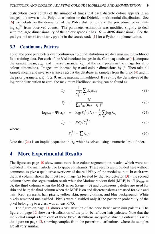
4 More Experimental Results
The figure on page 10 show some more face colour segmentation results, which were not
included in the main article due to space constraints. These results are provided here without
comment, to give a qualitative overview of the reliability of the model output. In each row,
the first column shows the input face image (as located by the face detector [3]); the second
column shows the segmentation result when the Markov random field (MRF) is off (kMRF =0); the third column when the MRF is on (kMRF = 3) and continuous palettes are used for
skin and hair; the final column when the MRF is on and discrete palettes are used for skin and
hair. Red represents hair pixels, yellow skin, green clothing, and blue background. White
pixels remained unclassified. Pixels were classified only if the posterior probability of the
pixel belonging to a class was at least 0.75.
The figure on page 11 shows a visualisation of the prior belief over skin palettes. The
figure on page 12 shows a visualisation of the prior belief over hair palettes. Note that the
individual samples from each of these two distributions are quite distinct. Contrast this with
the figure on page 13, showing samples from the posterior distributions, where the samples
are all very similar.

10 SCHEFFLER AND ODOBEZ: ADAPTIVE COLOUR MODELLING AND SEGMENTATION

SCHEFFLER AND ODOBEZ: ADAPTIVE COLOUR MODELLING AND SEGMENTATION 11
Y Pb
0 1
µ
9
426λ
0 1
µ
162
12871
λ
Pr
0 1
µ
114
8064
λ
The prior belief over skin palettes. Each plot shows a probability distribution (belief) over
the mean (µ) and inverse variance (λ ) of the normal distribution over a colour component.
The three colour components are luminance (Y), blue (Pb) and red (Pr).
Samples from the prior skin distribution. Each sample is a distribution over colours, repre-
sented here by a plot where the area devoted to each colour is proportional to its probability
of being observed.
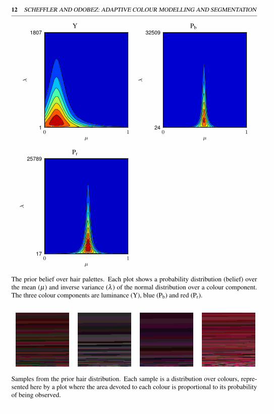
12 SCHEFFLER AND ODOBEZ: ADAPTIVE COLOUR MODELLING AND SEGMENTATION
Y Pb
0 1
µ
1
1807
λ
0 1
µ
24
32509
λ
Pr
0 1
µ
17
25789
λ
The prior belief over hair palettes. Each plot shows a probability distribution (belief) over
the mean (µ) and inverse variance (λ ) of the normal distribution over a colour component.
The three colour components are luminance (Y), blue (Pb) and red (Pr).
Samples from the prior hair distribution. Each sample is a distribution over colours, repre-
sented here by a plot where the area devoted to each colour is proportional to its probability
of being observed.
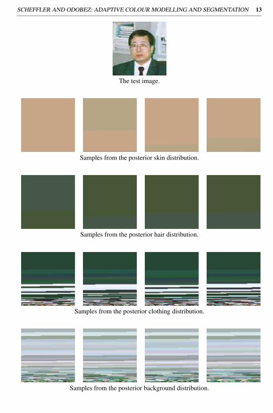
SCHEFFLER AND ODOBEZ: ADAPTIVE COLOUR MODELLING AND SEGMENTATION 13
The test image.
Samples from the posterior skin distribution.
Samples from the posterior hair distribution.
Samples from the posterior clothing distribution.
Samples from the posterior background distribution.
14 SCHEFFLER AND ODOBEZ: ADAPTIVE COLOUR MODELLING AND SEGMENTATION
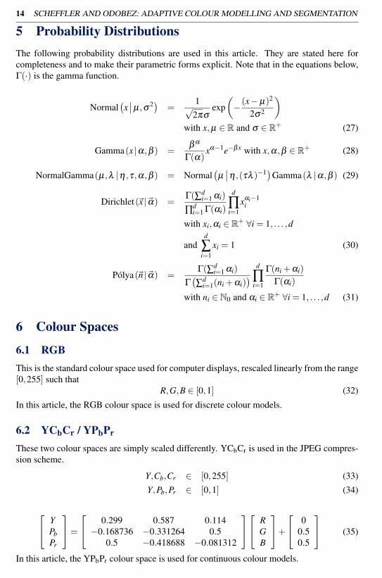
5 Probability Distributions
The following probability distributions are used in this article. They are stated here for
completeness and to make their parametric forms explicit. Note that in the equations below,
Γ(·) is the gamma function.
Normal(
x∣
∣µ,σ2)
=1√
2πσexp
(
− (x−µ)2
2σ2
)
with x,µ ∈ R and σ ∈ R+ (27)
Gamma(x |α,β ) =β α
Γ(α)xα−1e−βx with x,α,β ∈ R
+ (28)
NormalGamma(µ,λ |η ,τ,α,β ) = Normal(
µ∣
∣η ,(τλ )−1)
Gamma(λ |α,β ) (29)
Dirichlet(~x |~α) =Γ(∑d
i=1 αi)
∏di=1 Γ(αi)
d
∏i=1
xαi−1i
with xi,αi ∈ R+ ∀i = 1, . . . ,d
andd
∑i=1
xi = 1 (30)
Pólya(~n |~α) =Γ(∑d
i=1 αi)
Γ(
∑di=1(ni +αi)
)
d
∏i=1
Γ(ni +αi)
Γ(αi)
with ni ∈ N0 and αi ∈ R+ ∀i = 1, . . . ,d (31)
6 Colour Spaces
6.1 RGB
This is the standard colour space used for computer displays, rescaled linearly from the range
[0,255] such that
R,G,B ∈ [0,1] (32)
In this article, the RGB colour space is used for discrete colour models.
6.2 YCbCr / YPbPr
These two colour spaces are simply scaled differently. YCbCr is used in the JPEG compres-
sion scheme.
Y,Cb,Cr ∈ [0,255] (33)
Y,Pb,Pr ∈ [0,1] (34)
Y
Pb
Pr
=
0.299 0.587 0.114
−0.168736 −0.331264 0.50.5 −0.418688 −0.081312
R
G
B
+
0
0.50.5
(35)
In this article, the YPbPr colour space is used for continuous colour models.

SCHEFFLER AND ODOBEZ: ADAPTIVE COLOUR MODELLING AND SEGMENTATION 15
References
[1] Adaptive face colour modelling and segmentation project page. URL http://www.
idiap.ch/software/facecolormodel/.
[2] C. M. Bishop. Pattern Recognition and Machine Learning. Springer, 2006.
[3] Intel Corporation. OpenCV, version 2.0.0, October 2009. URL http://opencv.
willowgarage.com/wiki/.
[4] M. J. Jones and J. M. Rehg. Statistical color models with application to skin detection.
International Journal of Computer Vision, 46:81–96, 2002.
[5] M. I. Jordan, Z. Ghahramani, T. S. Jaakkola, and L. K. Saul. An introduction to varia-
tional methods for graphical models. Machine Learning, 37:183–233, 1999.
[6] T. Minka. Estimating a Dirichlet distribution. Technical report, 2009.