Joint Center for Housing Studies Harvard University

Developing a Leading Indicator for the Remodeling Industry Amal Bendimerad

April 2007 N07-1

Revised on April 17, 2008

© by Amal Bendimerad. All rights reserved. Short sections of text, not to exceed two paragraphs may be quoted without explicit permission provided that full credit, including © notice, is given to the source. Any opinions expressed are those of the author and not those of the Joint Center for Housing Studies of Harvard University or of any of the persons or organizations providing support to the Joint Center for Housing Studies.

1

Introduction

Homeowner remodeling expenditure is currently estimated at $280 billion dollars a year,

accounting for almost 40 percent of all residential construction and improvement spending and

more than 2 percent of the U.S. economy. Given the relative size and importance of the home

improvement industry, there is a surprisingly limited amount of data available on a consistent

and timely basis. The primary source of data, the Commerce Department’s quarterly survey

Expenditures for Residential Improvements and Repairs, commonly referred to as the C-50

report, is generally released several quarters after the reference period and the quarterly numbers

are unusually volatile. In an effort to improve the timeliness and stability of the data series, the

Joint Center for Housing Studies developed the Remodeling Activity Indicator (RAI), which

estimated current activity and expenditure. While this and other efforts helped provide the

industry with timely and stable estimates of remodeling activity, there was still no indicator to

provide a forward-looking approach to measuring the industry. There have been some attempts

at developing longer-term forecasts using econometric models, but there has been little work

done in the field of near-term projections of activity.

This paper describes the process for developing the Leading Indicator of Remodeling

Activity (LIRA), designed to estimate quarterly current and future home improvement

expenditures by homeowners. The indicator, measured as an annual rate-of-change of its

components, provides a short-term outlook of remodeling activity, with a horizon of three

quarters. Like all leading indicators, it is intended to also signal turning points in the business

cycle of the home improvement industry.

I. Research Context

Leading Indicators and Business Cycle Theory

One of the main characteristics of leading indicators is their ability to predict upturns and

downturns in activity. A leading indicator, therefore, must not only lead a sector in the business

cycle, but also be able to accurately predict its turning points. Accurately forecasting the cyclical

nature of an industry however, is difficult. For one thing, "cycles" is a rather misleading

concept, as the peaks and troughs don't tend to repeat at regular time intervals. The lengths (from

2

peak to peak or from trough to trough) vary, so cycles are not mechanical in their regularity.1

Moreover, the various drivers of a given industry can have different cycles, making it difficult to

understand what the aggregate effect will be. For these and other reasons, leading indicators can

be a tricky and sometimes a fairly inexact science. They do however, provide a good estimate of

trends and general levels of activity.

Several approaches to leading indicators have been produced in both academic and

industry literature. One of these approaches is the technique used by the Conference Board, the

organization that manages the most popular and widely-cited leading indicator on the U.S.

macroeconomy. This technique, which has been mimicked by many other efforts measuring

national and international macroeconomic and sector-specific activity, consists of building a

diffusion index based on the change of a series of input variables.2

Another approach, spearheaded by Stock and Watson, utilizes a vector autoregressive

technique to specify a statistical model. The model is based on the notion that the co-movements

in many macroeconomic time series can be captured by a single unobserved variable representing

the overall state of the economy. The result, named the Experimental Coincident Indicator,

measures the probability of a recession in a given time period. The Experimental Leading Index

(XLI), based on seven leading indicators, is a forecast of the percentage growth of the coincident

index (at an annual rate) for the following six months.3 While the Stock Watson leading indicator

(XLI) and related series were retired in December 2003, several successors using similar

methodologies are available, most notably the Chicago Fed National Activity Index (CFNAI).

II. Research Challenges

Introduction of new data series

The development of this project was borne mostly from the need for a reliable leading

indicator for home improvement activity: however, the recent introduction of several new,

relevant data series made this effort particularly important and timely. Several new data series

relating to remodeling activity have recently been released, contributing to a relatively barren

1 Banerji, Anirvan, 1999. For a more complete description of modeling business cycles please see: Gordon, Robert 2005; Klein et al. 1990; Moore, Geoffrey 1983; and Romer, Christina 1999. 2 See Conference Board website (www.conference-board.org) for further detail on methodology. 3 See Stock, J. and M. Watson 1990 and 2003.

3

landscape of remodeling-specific data. Because data specific to home improvement activity is so

limited, capturing remodeling trends through these sources provides a unique opportunity.

In recent years, the National Association of Home Builders has produced the Remodeling

Market Index (RMI), a survey that asks professional remodelers about their current and future

business expectations. Similarly, in March of 2005, the National Association of Realtors debuted

a new Pending Home Sales Index (PHSI), which measures home purchase contract activity.

Because of their potential ability to measure remodeling activity, and particularly because of

their potential lead of this activity, the consideration of these and other variables is important.

Also, beginning with the third quarter of 2006, Freddie Mac began releasing quarterly

cash-out volume statistics for home mortgage refinancing. The data are available for the U.S.

from 1993 and include statistics on cash-out volume as a percentage of refinance originations

volume, estimates of total home equity cashed out, and estimates of the total increase in first lien

mortgage debt due to cash-outs and consolidation of existing second mortgages. Studies4 have

shown that a significant share of homeowner improvements is financed through cash-out

withdrawals from the refinancing of their home.

The challenge presented with these data series however, is that the historical time series

is very short. Short data series can present a number of problems in developing leading

indicators, and most notably, the relationship between the indicator and measured outcome may

be volatile. For that reason, some econometric or statistical techniques become difficult to

implement, and the results are challenging to interpret. Given the priority in the inclusion of the

new data series, however evaluating the tradeoff was necessary.

Volatility of C-50 Series

Exacerbating the difficulty in measuring the cyclical nature of remodeling activity is the

unusual volatility of the C-50 data. Because the C-50 numbers are the only publicly-released

national series available on a quarterly basis, the leading indicator was designed to lead the C-50

numbers. As Figure 1 below reveals, the C-50 data series is a particularly volatile series, with

reason to believe that much of this volatility is random.

The data for the household survey of the C-50 are obtained from household members as

part of the Consumer Expenditure Surveys (CES) conducted by the Bureau of Labor Statistics.

4 See Martin-Guerrero, Alvaro 2004; Canner et al. 2002.

4

The expenditures covered by the survey are those that respondents can be expected to recall

fairly accurately for three months or less, including expenditures for maintenance, repairs and

improvements of residential property. Each sample household is interviewed once per quarter

for five consecutive quarters.5

One of the major sources of volatility of the C-50 numbers is the size of the sample. The

survey targets about 7,500 housing units for interviews per quarter, of which about 4,000 are

owner-occupied. This sample is then weighted up to the national total. This effort is

problematic for a few reasons. For one, a smaller sample has a higher sample error. Sampling

error reflects the fact that only a subset was surveyed rather than the entire population. Smaller

samples, therefore, have a higher likelihood of either missing households with large

expenditures, or including them and therefore overestimating national expenditures. Because the

CES is designed to gather information on small, frequent purchases such as food and clothing, it

is often hard to get an accurate measure of large, relatively infrequent expenditures such as

remodeling. In 2005, for example, remodeling expenditures of $20,000 accounted for over 60

percent of annual expenditures. Likewise, expenditures of $50,000 accounted for over 40

percent of annual expenditures.6 Only about 2.5 percent of homeowners report levels of

expenditure of $20,000 or more, and less than one percent of homeowners account for spending

of $50,000 or more. For example, if a household in the survey undertakes a very large

remodeling project in a given quarter and that household has a high weight to the national total,

remodeling expenditures in that quarter will be very high. If that same household has no activity

the next quarter, the weighted totals will drop significantly.

5 See U.S. Census website, “Survey Methods and Reliability of Data” appendix. 6 JCHS tabulations of the 2005 American Housing Survey.

5

Figure 1: Quarterly Home Improvement Data is Particularly Volatile

100

150

20019

89 -

Q1

1990

- Q

1

1991

- Q

1

1992

- Q

1

1993

- Q

1

1994

- Q

1

1995

- Q

1

1996

- Q

1

1997

- Q

1

1998

- Q

1

1999

- Q

1

2000

- Q

1

2001

- Q

1

2002

- Q

1

2003

- Q

1

2004

- Q

2

To

tal

ho

me i

mp

rove

men

t an

d r

ep

air

exp

en

dit

ure

s b

y o

wn

ers

(B

ilio

ns

$)

Recession Homeowner Home Improvement Spending

Source: U.S. Census Bureau, Construction Statistics, C50 series

Furthermore, the C-50 series does not seem to consistently exhibit the same cyclical

nature of the broader economy. In the two national economic recessions since 1990, the C-50

showed very small declines. To some extent, this may be an example of the particularly resilient

nature of the remodeling industry. On the other hand, there may be issues in the measurement

and methodology of calculating the C-50 that are masking “real-life” downturns that are more in

line with the broader economy. In both cases, this presents a particular challenge in the

development of the leading indicator.

If the leading indicator is to use the C-50 as it benchmark, and attempts to predict its

cycles, this task becomes increasingly difficult with the particularly high random volatility of the

data series. For that reason, the methodology in developing the LIRA is one that attempts to

predict the general trend of activity, but reduce some of the random volatility of the benchmark

series to create a series that is more stable and hopefully more closely aligned with actual activity

and expenditure levels.

6

III. Developing the Leading Indicator: The Theoretical Approach

Overview of the Method of Developing the Leading Indicator

The LIRA was created to provide the home improvement industry with a timely and

accurate estimation of changes in spending activity by homeowners, as well as an estimate of

near-term activity, with a horizon of three quarters. On a quarterly basis, the LIRA tracks the

annual volume of homeowner expenditures in home improvements and repairs from the C-50

series using the four-quarter moving averages of several indicators that are associated with

homeowner maintenance and improvement activity. The annual rates-of-change for the input

components of the LIRA are lagged differentially, meaning that they have a different timing

relationship with home improvement spending. This relationship was determined by evaluating

which lag produced the best correlation with annual rate-of-change of homeowner remodeling

expenditures. The input variables were then weighted according to their correlation with the C-

50 series and their volatility. Finally, the components were integrated into one four-quarter rate

of change that constituted the LIRA.

Identification of Candidates for Input Variables

The first phase of the project involved building a list of potential inputs. The

identification of input components derived from the following criteria: they needed to have

direct or indirect influence on remodeling activity, and they needed to have a significant lead on

the activity. In other words, they needed to be drivers of remodeling activity. To begin, a list of

broad categories of indicators that were thought to be drivers of the remodeling industry was

established. These categories were as follows: consumer plans for future remodeling,

professional contractor sentiment on future business activity, housing market activity,

macroeconomic conditions, financial market conditions, and consumer confidence.

Consumer plans for future remodeling have obvious implications for the outlook on the

remodeling market. It is also important to capture housing market activity, as remodeling

expenditure tends to move in tandem with other housing market activity. In addition to

remodeling- and housing-specific inputs, some macroeconomic and financial indicators were

included to capture broader economic trends. While the remodeling market tends to move closely

with the home building market, remodeling activity does tend to be a bit more resilient than new

construction. The inclusion of other economic factors therefore allows us to capture future

7

changes to the remodeling industry that are not present in other aspects of the housing market.

Additionally, macroeconomic and financial health variables capture some of the cyclicality in the

general economy that remodeling-specific variables might not.

8

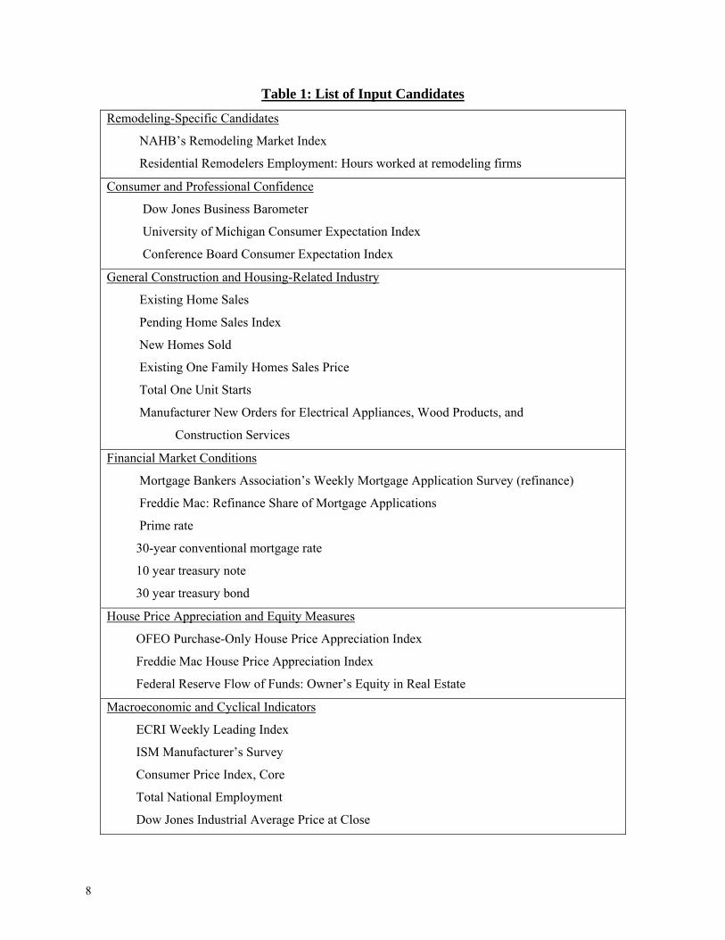
Table 1: List of Input Candidates

Remodeling-Specific Candidates

NAHB’s Remodeling Market Index

Residential Remodelers Employment: Hours worked at remodeling firms

Consumer and Professional Confidence

Dow Jones Business Barometer

University of Michigan Consumer Expectation Index

Conference Board Consumer Expectation Index

General Construction and Housing-Related Industry

Existing Home Sales

Pending Home Sales Index

New Homes Sold

Existing One Family Homes Sales Price

Total One Unit Starts

Manufacturer New Orders for Electrical Appliances, Wood Products, and

Construction Services

Financial Market Conditions

Mortgage Bankers Association’s Weekly Mortgage Application Survey (refinance)

Freddie Mac: Refinance Share of Mortgage Applications

Prime rate

30-year conventional mortgage rate

10 year treasury note

30 year treasury bond

House Price Appreciation and Equity Measures

OFEO Purchase-Only House Price Appreciation Index

Freddie Mac House Price Appreciation Index

Federal Reserve Flow of Funds: Owner’s Equity in Real Estate

Macroeconomic and Cyclical Indicators

ECRI Weekly Leading Index

ISM Manufacturer’s Survey

Consumer Price Index, Core

Total National Employment

Dow Jones Industrial Average Price at Close

9

IV. Developing the Leading Indicator: Calculation Methodology

Finalizing Input Variables

The second phase of the project deals with statistical analysis. Once the long list of

potential variables was established, a series of tests were undertaken. The inclusion of potential

inputs was based on three considerations: economic significance, statistical relationship, and

timeliness of the release relative to that of the indicator. When testing statistics variables, there

are a few statistical tests that can be utilized. The first and most common is correlation analysis.

Correlations allow one to understand how closely the two data series move together. While it

does not necessarily reveal the explanatory power of the variable, it does associate the trends of

the two series. Thus, it was important to find indicators that led remodeling activity and had

high correlations with the indicator.

Upon running correlations, the best were chosen from each category of candidates. In

some cases, there were no candidates whose correlation was strong enough, and there were

therefore no candidates selected from that category. The variables with the highest

concentrations were then tested in a regression analysis context, checking their significance with

a t-statistic, as well as their explanatory power on the reference series.

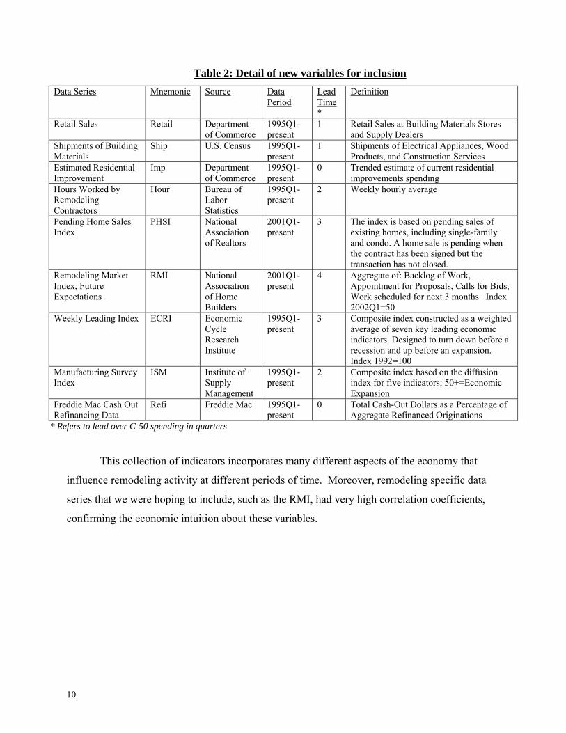
After the testing potential inputs, the final list consists of nine inputs with varying leads

(see Table 2).

10

Table 2: Detail of new variables for inclusion Data Series Mnemonic Source Data

Period Lead Time*

Definition

Retail Sales Retail Department of Commerce

1995Q1-present

1 Retail Sales at Building Materials Stores and Supply Dealers

Shipments of Building Materials

Ship U.S. Census 1995Q1-present

1 Shipments of Electrical Appliances, Wood Products, and Construction Services

Estimated Residential Improvement

Imp Department of Commerce

1995Q1-present

0 Trended estimate of current residential improvements spending

Hours Worked by Remodeling Contractors

Hour Bureau of Labor Statistics

1995Q1-present

2 Weekly hourly average

Pending Home Sales Index

PHSI National Association of Realtors

2001Q1-present

3 The index is based on pending sales of existing homes, including single-family and condo. A home sale is pending when the contract has been signed but the transaction has not closed.

Remodeling Market Index, Future Expectations

RMI National Association of Home Builders

2001Q1-present

4 Aggregate of: Backlog of Work, Appointment for Proposals, Calls for Bids, Work scheduled for next 3 months. Index 2002Q1=50

Weekly Leading Index ECRI Economic Cycle Research Institute

1995Q1-present

3 Composite index constructed as a weighted average of seven key leading economic indicators. Designed to turn down before a recession and up before an expansion. Index 1992=100

Manufacturing Survey Index

ISM Institute of Supply Management

1995Q1-present

2 Composite index based on the diffusion index for five indicators; 50+=Economic Expansion

Freddie Mac Cash Out Refinancing Data

Refi Freddie Mac 1995Q1-present

0 Total Cash-Out Dollars as a Percentage of Aggregate Refinanced Originations

* Refers to lead over C-50 spending in quarters

This collection of indicators incorporates many different aspects of the economy that

influence remodeling activity at different periods of time. Moreover, remodeling specific data

series that we were hoping to include, such as the RMI, had very high correlation coefficients,

confirming the economic intuition about these variables.

11

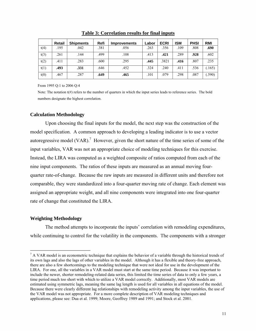
Table 3: Correlation results for final inputs Retail Shipments Refi Improvements Labor ECRI ISM PHSI RMI t(4) .195 .042 .381 .056 .263 .356 .109 .808 .690

t(3) .261 .144 .499 .108 .413 .421 .289 .928 .602

t(2) .411 .283 .600 .295 .445 .3821 .416 .807 .235

t(1) .493 .331 .646 .452 .324 .240 .411 .536 (.165)

t(0) .467 .287 .649 .465 .101 .079 .298 .087 (.590)

From 1995 Q:1 to 2006 Q:4

Note: The notation t(#) refers to the number of quarters in which the input series leads to reference series. The bold

numbers designate the highest correlation.

Calculation Methodology

Upon choosing the final inputs for the model, the next step was the construction of the

model specification. A common approach to developing a leading indicator is to use a vector

autoregressive model (VAR).7 However, given the short nature of the time series of some of the

input variables, VAR was not an appropriate choice of modeling techniques for this exercise.

Instead, the LIRA was computed as a weighted composite of ratios computed from each of the

nine input components. The ratios of these inputs are measured as an annual moving four-

quarter rate-of-change. Because the raw inputs are measured in different units and therefore not

comparable, they were standardized into a four-quarter moving rate of change. Each element was

assigned an appropriate weight, and all nine components were integrated into one four-quarter

rate of change that constituted the LIRA.

Weighting Methodology

The method attempts to incorporate the inputs’ correlation with remodeling expenditures,

while continuing to control for the volatility in the components. The components with a stronger

7 A VAR model is an econometric technique that explains the behavior of a variable through the historical trends of its own lags and also the lags of other variables in the model. Although it has a flexible and theory-free approach, there are also a few shortcomings to the modeling technique that were not ideal for use in the development of the LIRA. For one, all the variables in a VAR model must start at the same time period. Because it was important to include the newer, shorter remodeling-related data series, this limited the time series of data to only a few years, a time period much too short with which to utilize a VAR model correctly. Additionally, most VAR models are estimated using symmetric lags, meaning the same lag length is used for all variables in all equations of the model. Because there were clearly different lag relationships with remodeling activity among the input variables, the use of the VAR model was not appropriate. For a more complete description of VAR modeling techniques and applications, please see: Dua et al. 1999; Moore, Geoffrey 1989 and 1991; and Stock et al. 2001.

12

correlation with remodeling expenditures therefore have a higher weight in the LIRA

estimations. The nine components of the new indicator show a broad range of both correlation to

and timing with the C-50 series.

Table 4: Summary of Input Weights

The weight for each indicator is calculated using both the correlation and the inverse of the

variation for each component. Each component is weighted by the inverse of its standard

deviation, and by its correlation with the reference series. The weight can be expressed in terms of:

Σwi ni

Σni =1 wi

where w, refers to the average of the inverse of the standard deviation (1/STD) and the share of

the correlation coefficients for each element (n). The function for the indicator can be

summarized in the formula:

It0Wt0I + Rt1Wt1R + St1Wt1S + Lt2Wt2L + Et3Wt3E + Mt3Wt3M + Pt3Pt3H+Nt3Wt3 N+Ct0Wt3 0 (LIRAt0) = ΣWIRSLEMPNC

where I= improvement estimates; R= retail sales at building material and supply stores;

S=shipments of building materials; L=average hours worked weekly; E=ECRI’s weekly leading

index; M=ISM’s Manufacturing Index; P=pending home sales; N=remodeling market index; and

C=cashout measure.

Improvements Refi Retail Shipments ISM Labor ECRI PHSI RMI t (0) t(0) t (1) t (1) t (2) t (2) t (3) t (3) t (4)

Number of Observations 44 48 48 48 48 48 44 17 17

Average Value 1.06 1.10 1.08 1.03 1.01 .998 1.02 1.04 1.00

Standard Deviation 0.087 0.052 0.031 0.046 0.096 0.009 0.028 0.067 0.083

1/STD 11.55 19.34 32.07 21.59 10.38 113.94 35.88 14.93 12.01

Share of sum of 1/STD 4% 7% 12% 8% 4% 42% 13% 5% 4%

Correlation w/ C-50 0.4646 0.6499 0.4928 0.3305 0.4156 0.445 0.4218 0.928 0.6903 Share of sum of Correlation 10% 13% 10% 7% 9% 9% 9% 19% 14%

Final Weight 6.93% 10.27% 10.99% 7.39% 6.20% 25.57% 10.96% 12.34% 9.34%

13

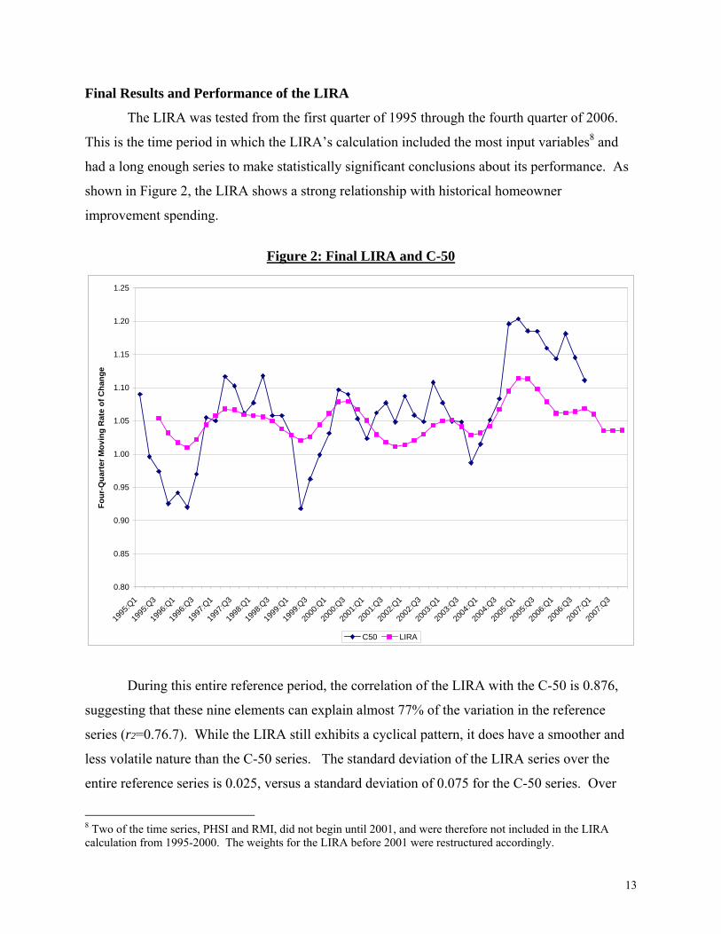
Final Results and Performance of the LIRA

The LIRA was tested from the first quarter of 1995 through the fourth quarter of 2006.

This is the time period in which the LIRA’s calculation included the most input variables8 and

had a long enough series to make statistically significant conclusions about its performance. As

shown in Figure 2, the LIRA shows a strong relationship with historical homeowner

improvement spending.

Figure 2: Final LIRA and C-50

0.80

0.85

0.90

0.95

1.00

1.05

1.10

1.15

1.20

1.25

1995

:Q1

1995

:Q3

1996

:Q1

1996

:Q3

1997

:Q1

1997

:Q3

1998

:Q1

1998

:Q3

1999

:Q1

1999

:Q3

2000

:Q1

2000

:Q3

2001

:Q1

2001

:Q3

2002

:Q1

2002

:Q3

2003

:Q1

2003

:Q3

2004

:Q1

2004

:Q3

2005

:Q1

2005

:Q3

2006

:Q1

2006

:Q3

2007

:Q1

2007

:Q3

Four

-Qua

rter

Mov

ing

Rat

e of

Cha

nge

C50 LIRA

During this entire reference period, the correlation of the LIRA with the C-50 is 0.876,

suggesting that these nine elements can explain almost 77% of the variation in the reference

series (r2=0.76.7). While the LIRA still exhibits a cyclical pattern, it does have a smoother and

less volatile nature than the C-50 series. The standard deviation of the LIRA series over the

entire reference series is 0.025, versus a standard deviation of 0.075 for the C-50 series. Over

8 Two of the time series, PHSI and RMI, did not begin until 2001, and were therefore not included in the LIRA calculation from 1995-2000. The weights for the LIRA before 2001 were restructured accordingly.

14

the reference period, the average growth rate of the LIRA is 4.98 percent, while the average

growth rate of the C-50 series is 6.44 percent.

Of course, the LIRA’s main objective is to anticipate turning points in the cycles of home

improvement spending. As seen in Figure 2, the LIRA demonstrates similar cyclicality to the C-50

series, albeit without as much volatility. During the time period between the third quarter of 1995

and the end of 2006, expenditures in remodeling reached four cyclical high points; the LIRA

anticipated three of the four. Moreover, during this period, remodeling expenditures had four

cyclical low points; in all four cases, the LIRA anticipated these contractions.

Figure 3: Final LIRA, Remodeling Expenditure, and GDP

0.9

0.95

1

1.05

1.1

1.15

1.2

1.25

1.3

1995

:Q3

1996

:Q1

1996

:Q3

1997

:Q1

1997

:Q3

1998

:Q1

1998

:Q3

1999

:Q1

1999

:Q3

2000

:Q1

2000

:Q3

2001

:Q1

2001

:Q3

2002

:Q1

2002

:Q3

2003

:Q1

2003

:Q3

2004

:Q1

2004

:Q3

2005

:Q1

2005

:Q3

2006

:Q1

2006

:Q3

2007

:Q1

2007

:Q3

Four

-Qua

rter

Mov

ing

Rat

e of

Cha

nge

C50 LIRA GDP The one point in which the LIRA diverges significantly from the C-50 series occurs during

the 2001-2002 time period. As a point of reference, Figure 3 plots remodeling expenditures along

with the two reference series. The period from 2001 to 2002 was an exceptional time in which the

remodeling industry held strong despite a recession in the economy. Because of historically low

interest rates and unusually high levels of home price appreciation, the remodeling and new

construction industries held strong even though GDP dipped.

15

As with any new research endeavor, the progression of the LIRA will be carefully

monitored. As time passes and more data points are added to the series, more robust statistical

tests can be performed. Moreover, future economic upturns and downtowns will allow for

further testing of the performance of the LIRA at various points in economic cycles. If need be,

minor revisions will be made to the LIRA as a result of new information.

V. Conclusion

The Leading Remodeling Activity Indicator (LIRA) was developed as a measure of near-

term activity in the home remodeling industry. As the first of its kind, its intended purpose is to

predict household remodeling spending with a three-quarter horizon. Like any leading indicator,

the LIRA’s main objective is to anticipate turning points in the industry cycle.

Development of the LIRA took place in two main phases. The first phase consisted of

developing a theoretical framework for the indicator and a list of potential candidates for

inclusion in the indicator. Candidates were chosen from a broad range of areas that are believed

to impact home remodeling activity, including consumer sentiment, general construction and

housing-related indicators, and macroeconomic variables.

The second part of the development of the leading indicator was a statistical exercise.

Potential candidates were tested using correlation analysis, and the best series in each broad

category was chosen. The inputs were then weighted using their relevance to the reference series

and their standard deviation. Finally, these inputs were consolidated into a comprehensive

growth rate measuring remodeling activity.

The final result is an indicator that does a good job of tracking remodeling activity. The

final LIRA has a cyclical nature which coincides well with cycles in the C-50 data. More

importantly, the historical series anticipates turning points in this data series well. While the

LIRA maintains the same patterns as the reference series, it has a smoother pattern, dulling some

of the apparently random volatility that appears in the reference series.

16

References

Banerji, Anirvan. The Lead Profile and Other Non-Parametric Tools to Evaluate Survey Series as Leading Indicators. 1999. Prepared for the CIRET Conference, New Zealand.

Canner, G., K. Dynan, and W. Passmore. 2002. Mortgage Refinancing in 2001 and Early 2002.

Federal Reserve Bulletin (December), pp. 469–481. Diebold, Francis X. and Glenn Rudebusch. 1991. Forecasting Output with a Composite Leading

Index. Journal of the American Statistical Association 86(415): 603-610. Dua, Pami, Stephen Miller, and David Smyth. 1999. Using Leading Indicators to Forecast US

Home Sales in a Bayesian VAR Framework. Journal of Real Estate Finance and Economics 18(2): 191-205.

Gordon, Robert. What Caused the Decline In U.S. Business Cycle Volatility? 2005. Prepared for

The Conference on the Changing Nature of the Business Cycle. Sidney, Australia. Klein, Philip. et al. Analyzing Modern Business Cycles: Essays Honoring Geoffrey H. Moore,

1990. M.E. Sharpe Publishing, Armonk, New York. Martin-Guerrero, Alvaro. Home Improvement Finance: Evidence from the 2001 Consumer

Practices Survey. 2003. Joint Center for Housing Studies Research Note N03-1, Cambridge, MA.

Megna, Robert and Qiang Xu. Forecasting the New York State Economy: The Coincident and

Leading Indicators Approach. New York Division of the Budget. Albany, New York. Moore, Geoffrey. Business Cycles, Inflation, and Forecasting. 1983. National Bureau of

Economic Research, Inc. Ballinger Publishing Company, Cambridge, MA. Moore, Geoffrey and Kajal Lahiri. 1991. Leading Economic Indicators: New Approaches and

Forecasting Records. Cambridge University Press. New York, NY. Moore, Geoffrey and Allan Layton. 1989. Leading Indicators for the Service Sector. Journal of

Business and Economic Statistics. 7(3): 379-386. Romer, Christina. 1999. Changes in Business Cycles: Evidence and Explanations. Journal of

Economic Perspectives 13(1): 55-74. The Conference Board. www.conference-board.org. 2005 Stock, James and Mark Watson. 1990. New Indexes of Coincident and Leading Economic

Indicators. National Bureau of Economic Research Working Paper No. R1380. Stock, James and Mark Watson. 2001. Vector Autoregressions. Journal of Economic

Perspectives 15(4): 101-115.

17

Stock, James and Mark Watson. 2003. How Did Leading Indicator Forecasts Perform During the

2001 Recession? Federal Reserve Bank of Richmond Economic Quarterly 89(3): 71-89.

18

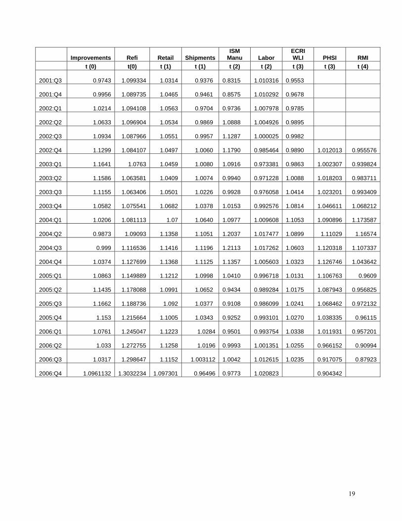
Appendix 1: Raw Data to Final Input Variables (4-quarter moving rates of change)

Improvements Refi Retail Shipments ISM

Manu Labor ECRI WLI PHSI RMI

t (0) t(0) t (1) t (1) t (2) t (2) t (3) t (3) t (4)

1995:Q1 1.0756 1.093032 1.1258 1.0938 1.0798 1.002557

1.0054

1995:Q2 1.0195 1.095964 1.1014 1.0565 0.9963 0.99272

1.0087

1995:Q3 0.9611 1.088249 1.0685 1.0336 0.9187 0.989057

1.0205

1995:Q4 0.9242 1.079741 1.0451 1.0127 0.8539 0.985841

1.0340

1996:Q1 0.9199 1.070246 1.028 0.9940 0.8245 0.986046

1.0406

1996:Q2 0.9622 1.071033 1.0378 1.0137 0.8744 0.993711

1.0430

1996:Q3 1.0732 1.079798 1.0578 1.0212 0.9266 0.996008

1.0400

1996:Q4 1.1851 1.085852 1.0682 1.0350 1.0149 0.997204

1.0397

1997:Q1 1.2309 1.093938 1.0794 1.0595 1.0993 0.999282

1.0372

1997:Q2 1.1942 1.098834 1.0831 1.0552 1.1069 1.000561

1.0458

1997:Q3 1.0874 1.094036 1.0795 1.0572 1.1227 1.005254

1.0502

1997:Q4 1.0106 1.089515 1.0784 1.0619 1.0993 1.009058

1.0480

1998:Q1 0.9959 1.080123 1.0738 1.0612 1.0570 1.005639

1.0532

1998:Q2 1.0136 1.070184 1.0646 1.0628 1.0141 0.996215

1.0361

1998:Q3 1.0244 1.065644 1.0586 1.0568 0.9536 0.987069

1.0197

1998:Q4 0.9964 1.061664 1.0622 1.0427 0.9044 0.982219

1.0097

1999:Q1 0.9535 1.066617 1.0707 1.0314 0.8983 0.982877

0.9992

1999:Q2 0.9264 1.0719 1.0806 1.0283 0.9314 0.992841

1.0060

1999:Q3 0.9796 1.083584 1.0894 1.0289 0.9930 1.000573

1.0213

1999:Q4 1.0956 1.094113 1.092 1.0332 1.0835 1.0047

1.0351

2000:Q1 1.1948 1.103156 1.0951 1.0463 1.1167 1.009822

1.0362

2000:Q2 1.2632 1.110538 1.0884 1.0423 1.0967 1.009019

1.0335

2000:Q3 1.2065 1.113892 1.0731 1.0309 1.0476 1.010557

1.0184

2000:Q4 1.1019 1.117471 1.0521 1.0113 0.9545 1.013236

0.9934

2001:Q1 1.0199 1.110487 1.0278 0.9659 0.8739 1.014094

0.9806

2001:Q2 0.9654 1.105354 1.0257 0.9424 0.8326 1.013351

0.9632

19

Improvements Refi Retail Shipments ISM

Manu Labor ECRI WLI PHSI RMI

t (0) t(0) t (1) t (1) t (2) t (2) t (3) t (3) t (4)

2001:Q3 0.9743 1.099334 1.0314 0.9376 0.8315 1.010316

0.9553

2001:Q4 0.9956 1.089735 1.0465 0.9461 0.8575 1.010292

0.9678

2002:Q1 1.0214 1.094108 1.0563 0.9704 0.9736 1.007978

0.9785

2002:Q2 1.0633 1.096904 1.0534 0.9869 1.0888 1.004926

0.9895

2002:Q3 1.0934 1.087966 1.0551 0.9957 1.1287 1.000025

0.9982

2002:Q4 1.1299 1.084107 1.0497 1.0060 1.1790 0.985464

0.9890 1.012013 0.955576

2003:Q1 1.1641 1.0763 1.0459 1.0080 1.0916 0.973381

0.9863 1.002307 0.939824

2003:Q2 1.1586 1.063581 1.0409 1.0074 0.9940 0.971228

1.0088 1.018203 0.983711

2003:Q3 1.1155 1.063406 1.0501 1.0226 0.9928 0.976058

1.0414 1.023201 0.993409

2003:Q4 1.0582 1.075541 1.0682 1.0378 1.0153 0.992576

1.0814 1.046611 1.068212

2004:Q1 1.0206 1.081113 1.07 1.0640 1.0977 1.009608

1.1053 1.090896 1.173587

2004:Q2 0.9873 1.09093 1.1358 1.1051 1.2037 1.017477

1.0899 1.11029 1.16574

2004:Q3 0.999 1.116536 1.1416 1.1196 1.2113 1.017262

1.0603 1.120318 1.107337

2004:Q4 1.0374 1.127699 1.1368 1.1125 1.1357 1.005603

1.0323 1.126746 1.043642

2005:Q1 1.0863 1.149889 1.1212 1.0998 1.0410 0.996718

1.0131 1.106763 0.9609

2005:Q2 1.1435 1.178088 1.0991 1.0652 0.9434 0.989284

1.0175 1.087943 0.956825

2005:Q3 1.1662 1.188736 1.092 1.0377 0.9108 0.986099

1.0241 1.068462 0.972132

2005:Q4 1.153 1.215664

1.1005 1.0343 0.9252 0.993101

1.0270 1.038335 0.96115

2006:Q1 1.0761 1.245047

1.1223 1.0284 0.9501 0.993754

1.0338 1.011931 0.957201

2006:Q2 1.033 1.272755

1.1258 1.0196 0.9993 1.001351

1.0255 0.966152 0.90994

2006:Q3 1.0317 1.298647

1.1152 1.003112 1.0042 1.012615 1.0235 0.917075 0.87923

2006:Q4 1.0961132 1.3032234 1.097301 0.96496 0.9773 1.020823 0.904342