Setembro 2008

Joint Detection-Estimation of Brain Activity in fMRI using Graph Cuts

Joana Maria Rosado da Silva Coelho

Dissertação para obtenção do Grau de Mestre em

Engenharia Biomédica

Júri Presidente: Prof. Patrícia Margarida Piedade Figueiredo

Orientadores: Prof. João Miguel Raposo Sanches

Prof. Martin Hagen Lauterbach

Vogal: Prof. Mário Alexandre Teles de Figueiredo

Acknowledgments

I would like to thank my IST supervisor, Prof. João Sanches, for his constant involvement, effort andadvice throughout these six months. I also wish to thank to my FML supervisor, Dr. Martin Lauterbach,for all the availability, support and patience in answering all my questions and to those who have patientlylaid in the scanner for my experiments. I would like to thank the Institute for Systems and Robotics fortheir funding in publishing part of this thesis in international conferences and journal. I also wish to thankProf. Patricia Figueiredo for the occasional explanations. A special thanks to José Santos for helpingme in generating some of the figures in this thesis and for always being there. And also to my futurebrother-in-law, Deny Bobula, for his patience in reading and trying to correct any language mistakes ofthis thesis even being many miles away. And finally, any endeavour of this kind is not possible withoutthe patience, constant support and encouragement of my family and loved ones, to whom I dedicate thisthesis.

2

Abstract

The BOLD technique is an fMRI method that allows the detection of brain activated regions afterapplication of an external stimulus. This technique is based on the assumption that the metabolismincreases in activated areas as well as the oxygen uptake. Analising this information is a challengingproblem because the BOLD signal is very noisy and the task-related signal changes are small in amplitude.Therefore, the detection of temporal correlations with the applied stimulus requires statistical algorithmsto understand if the changes on the BOLD signal are related with the applied stimulus. The traditionalapproach needs the tuning of a parameter by a medical doctor which makes it impossible to be completelyautomatic.

In this thesis, a new Bayesian parameter-free method to detect brain activated areas in fMRI isdescribed. The traditional estimation and inference steps are joint together and the neural activitydetection, characterised by binary variables, is obtained simultaneously with an hemodynamic responsefunction (HRF) estimation and a drift removal processing. Finally, a spatial correlation step with GraphCuts is introduced to improve the detection of brain activity. This approach brings several advantagessince the activity detection is performed iteratively, benefiting from the adaptive HRF estimation anddrift removal. Moreover, the proposed method succeeds in providing local, space variant HRF estimation,an important physiologic characteristic.

Synthetic Monte Carlo tests are performed demonstrating the robustness of the algorithm. Finally,examples using real data are presented and compared with some results from the SPM-GLM.

Keywords: fMRI, Bayesian Models, Activation Detection, Hemodynamic Response,Spatial Correlation, Drift Removal.

3

Resumo

A aquisição de sinal BOLD (técnica de fMRI) permite a detecção de regiões cerebrais activadas após aaplicação de um estímulo externo. Esta técnica é baseada na hipótese de ocorrência de um aumento dometabolismo numa área que é activada, existindo consequentemente um aumento do aporte de oxigénio.Analisar este tipo de sinal é um desafio pois o sinal BOLD tem muito ruído e as suas variações são muitopequenas em amplitude. Assim, a detecção de correlação temporal necessita de algoritmos estatísticospara decidir se as variações no sinal estão relacionadas com o estímulo aplicado. A abordagem tradi-cional necessita do ajuste de um parâmetro por um médico tornando-a impossível de ser completamenteautomática.

Nesta tese é descrito um novo método Bayesiano, livre de parâmetros, capaz de detectar áreas cerebraisactivadas. Os tradicionais passos de estimação e inferência são realizados em conjunto, de forma a detectara actividade neuronal (caracterizada por variáveis binárias) simultaneamente com a estimação da funçãode resposta hemodinâmica (HRF) e a remoção do drift. Por fim, é introduzida correlação espacial comGraph Cuts para melhorar a detecção de actividade cerebral. Esta abordagem traz diversas vantagensvisto que a detecção de actividade é realizada iterativamente, beneficiando simultaneamente da estimaçãoadaptativa da HRF e da remoção do drift. O método proposto realiza, ainda, uma estimativa da HRFvariante no espaço, importante característica fisiológica.

A robustez do algoritmo é demonstrada usando testes sintéticos de Monte Carlo. Por fim, são apre-sentados exemplos usando dados reais e comparados com os resultados do SPM-GLM.

Keywords: fMRI, Modelos Bayesianos, Detecção de Activação, Resposta Hemodinâmica,Correlação Espacial, Remoção de Drift.

4

Contents

Acknowledgments 2

Abstract 3

Resumo 4

List of Abbreviations 7

1 Introduction 101.1 Objectives . . . . . . . . . . . . . . . . . . . . . . . . . . . . . . . . . . . . . . . . . . . . . 131.2 Original Contributions . . . . . . . . . . . . . . . . . . . . . . . . . . . . . . . . . . . . . . 141.3 Thesis Organization . . . . . . . . . . . . . . . . . . . . . . . . . . . . . . . . . . . . . . . 14

2 Literature Review 152.1 Classical and Bayesian Models . . . . . . . . . . . . . . . . . . . . . . . . . . . . . . . . . 15

2.1.1 Classical Models . . . . . . . . . . . . . . . . . . . . . . . . . . . . . . . . . . . . . 152.1.2 Bayesian Models . . . . . . . . . . . . . . . . . . . . . . . . . . . . . . . . . . . . . 18

2.2 Modelling Spatial Correlation . . . . . . . . . . . . . . . . . . . . . . . . . . . . . . . . . . 192.3 Modelling Slow Variation Drift . . . . . . . . . . . . . . . . . . . . . . . . . . . . . . . . . 20

3 Proposed Method 223.1 Notation . . . . . . . . . . . . . . . . . . . . . . . . . . . . . . . . . . . . . . . . . . . . . . 223.2 Model and problem formulation . . . . . . . . . . . . . . . . . . . . . . . . . . . . . . . . . 233.3 Bayesian Analysis . . . . . . . . . . . . . . . . . . . . . . . . . . . . . . . . . . . . . . . . . 25

3.3.1 Initializations . . . . . . . . . . . . . . . . . . . . . . . . . . . . . . . . . . . . . . . 263.3.2 Step One: b estimation . . . . . . . . . . . . . . . . . . . . . . . . . . . . . . . . . 283.3.3 Step Two: h estimation . . . . . . . . . . . . . . . . . . . . . . . . . . . . . . . . . 283.3.4 Step Three: d estimation . . . . . . . . . . . . . . . . . . . . . . . . . . . . . . . . 283.3.5 Step Four: Spatial Correlation . . . . . . . . . . . . . . . . . . . . . . . . . . . . . 29

4 Experimental Results 314.1 Synthetic Data . . . . . . . . . . . . . . . . . . . . . . . . . . . . . . . . . . . . . . . . . . 31

4.1.1 Brain Activation Detection . . . . . . . . . . . . . . . . . . . . . . . . . . . . . . . 314.1.2 Hemodynamic Response Function Estimation . . . . . . . . . . . . . . . . . . . . . 334.1.3 Drift Removal . . . . . . . . . . . . . . . . . . . . . . . . . . . . . . . . . . . . . . . 34

4.2 Real Data . . . . . . . . . . . . . . . . . . . . . . . . . . . . . . . . . . . . . . . . . . . . . 35

5 Conclusion and Future Work 40

Bibliography 41

5

6 Appendices 456.1 EMBC2008 Published Paper . . . . . . . . . . . . . . . . . . . . . . . . . . . . . . . . . . 456.2 RecPad Submitted Abstract . . . . . . . . . . . . . . . . . . . . . . . . . . . . . . . . . . . 50

6

List of Abbreviations

AWGN Additive White Gaussian NoiseBOLD Blood-Oxygenation-Level-DependentCBF Cerebral Blood FlowCBV Cerebral Blood VolumeEPI Echo-Planar ImagingEV Explanatory Variable

fMRI Functional Magnetic Resonance ImagingGE Gradient-Echo

GLM General Linear ModelHb Deoxygenated Hemoglobine

HbO2 Oxygenated HemoglobineHRF Hemodynamic Response Functioni.i.d Independent and Identically DistributedLTI Linear Time Invariant

MAP Maximum A PosterioriMRI Magnetic Resonance ImagingMRF Markov Random Field

RF Radio FrequencyRFT Random Field TheorySC Spatial Correlation

SNR Signal-to-Noise RatioSPM Statistical Parametric Mapping

SPM-Drift-GC SPM Bayesian framework with Drift removal and GC algorithmSPM-GC SPM Bayesian framework with GC algorithm

TR Time of RepetitionVoxel Volume Element

7

List of Figures

1.1 Representation of a theoretical hemodynamic response. . . . . . . . . . . . . . . . . . . . . 111.2 Schematic diagram of the fMRI data set: an example of an applied paradigm and the

BOLD response acquired. . . . . . . . . . . . . . . . . . . . . . . . . . . . . . . . . . . . . 121.3 Schematic diagram of different processing steps after fMRI data acquisition . . . . . . . . 13

2.1 Example of a time course from a visual stimulation experiment . . . . . . . . . . . . . . . 162.2 Schematic diagram of the GLM procedure . . . . . . . . . . . . . . . . . . . . . . . . . . . 172.3 Schematic representation of an unfiltered time course from an activated voxel and its

decomposition . . . . . . . . . . . . . . . . . . . . . . . . . . . . . . . . . . . . . . . . . . . 21

3.1 BOLD signal generation model . . . . . . . . . . . . . . . . . . . . . . . . . . . . . . . . . 233.2 Fluxogram with the main steps of the proposed iterative algorithm SPM-Drift-GC . . . . 273.3 Gamma Function chosen for hi initialization. . . . . . . . . . . . . . . . . . . . . . . . . . 27

4.1 Synthetic image of one of the applied stimuli representing a single BOLD slice image. . . 314.2 Graphics with the computed error probability for each noise level. . . . . . . . . . . . . . 324.3 Activation detection of a 4 epoch paradigm with SNR = 0.3 dB. . . . . . . . . . . . . . . 334.4 Example of an HRF estimation for SNR = 2 dB and 4 epochs paradigm. . . . . . . . . . 334.5 Example of the drift estimation for an SNR = 2 dB time course. . . . . . . . . . . . . . . 344.6 Example of an SNR = 2 dB time course with the real and estimated drift. . . . . . . . . 344.7 Example of a z signal from an SNR = 2 dB time course with 4 epochs. . . . . . . . . . . 354.8 Example of an estimated z signal and the original SNR = 2 dB time course. . . . . . . . 354.9 Real data activated regions of a verb generation and a motor paradigm. . . . . . . . . . . 364.10 Homunculus with motor representation of the brain areas responsible for a specific part of

the body. . . . . . . . . . . . . . . . . . . . . . . . . . . . . . . . . . . . . . . . . . . . . . 374.11 Anatomic representation of Wernicke’s and Broca’s areas. . . . . . . . . . . . . . . . . . . 374.12 Example of a time course from a new detected area by SPM-Drift-GC for the motor task

paradigm. . . . . . . . . . . . . . . . . . . . . . . . . . . . . . . . . . . . . . . . . . . . . . 384.13 Example of a time course from a new detected area by SPM-Drfit-GC for the verb gener-

ation paradigm. . . . . . . . . . . . . . . . . . . . . . . . . . . . . . . . . . . . . . . . . . . 384.14 Examples of two different estimated HRF from two different activated voxels. . . . . . . . 394.15 Example of an estimated drift and the correspondent noisy time course. . . . . . . . . . . 39

8

List of Tables

3.1 List of Notation . . . . . . . . . . . . . . . . . . . . . . . . . . . . . . . . . . . . . . . . . . 223.2 Prototype algorithm . . . . . . . . . . . . . . . . . . . . . . . . . . . . . . . . . . . . . . . 30

4.1 Description of the paradigms applied to the subjects . . . . . . . . . . . . . . . . . . . . . 36

9

Chapter 1

Introduction

What does the human body look like on the inside? For ages people have been curious about the insideof the human body and the surgery solution is not the most common way to discover it anymore. Arefinement of this procedure might be using an endoscope which conveys an image to a display device. Butboth methods are invasive techniques, which have the potential to cause damage or trauma to the body.Nowadays, medical imaging has been widely used with the objective of seeing the inside of the humanbody in a less invasive way. There are different medical imaging modalities such as radiographic imaging,nuclear medicine imaging, ultrasound imaging and magnetic resonance imaging that allow assessment ofthe different characteristics of the interior of the human body. From this wide range, Magnetic ResonanceImaging (MRI) is known as a noninvasive, excellent soft-tissue contrast and risk-free method [1].

MRI scanners use the property of nuclear magnetic resonance to create images. Several different nucleihave a net spin being magnetic resonance active but the most useful one for diagnosis is the hydrogennuclei since it is an abundant atom in the human body being present in substances such as water and fat.In a strong magnetic field, the nucleus of the hydrogen atom tends to align itself with the field. Giventhe extensive quantity of hydrogen atoms in the body, this tendency induces a net magnetization of thebody. It is then possible to selectively excite regions within the body, causing groups of atoms to tipaway from the magnetic field direction. When these protons return back into alignment with the field,they precess generating a radio frequency (RF) electromagnetic wave which can be acquired. There aremany pulse sequences available (time series of different excitatory pulses) that can be chosen accordingto the MRI modality desired and the type of tissue to be highlighted.

Among the different MRI modalities available, functional Magnetic Resonance Imaging (fMRI) isa recent and attractive method that makes it possible to detect which regions of the brain are beingactivated during a certain task. This modality is based on the assumption that activated regions presentincreased metabolic activity. Brain activity is assessed indirectly with high spatial resolution by detectingthe local hemodynamic changes in capillaries [2] and draining veins [3]. In fact, using this technique itis possible to establish brain activation maps in response to a specific stimulation such as performing anauditive, visual, verbal or motor task. To achieve this, specific stimulation is required, spontaneous brainactivity can not be measured [4]. Furthermore, fMRI investigators are not only interested in localizingbrain functions but seek to map the parts of the system that act in different combinations for differenttasks. This technique seems so powerful that is giving rise to an increasing interest from the scientificresearch community ranging from neuroscientists, neurologists, neuropsychologists, clinical psychologists,physiologists, radiologists and psychiatrists, as well as physicists, engineers and mathematicians. However,fMRI is not only a matter of academic curiosity but also has some medical applications as well, rangingfrom cognitive neuroscience, mapping of functional areas in damaged brain, defining mechanisms ofreorganization or compensation from injury [5]. This technique could be fundamental for presurgery

10

planning and functional neuronavigation, thorough characterization of some disease functional phenotypessuch as dyslexia and epilepsy, determining the effectiveness of some brain treatments, understanding thephysiological principles of neurological disorders and help in studying the brain organization of cognitiveand perceptual events [5,6].

In principle, fMRI measurements can be accomplished by different techniques but the Blood-Oxygenation-Level-Dependent (BOLD) technique is the most frequently used in the human brain often being referredas the standard-technique [4]. The method was first demonstrated in humans in the early 1990s in aresearch setting [7–9] where researchers established that a measurable MRI signal could be acquired invivo by using paramagnetic deoxyhemoglobin as an endogenous susceptibility contrast agent.

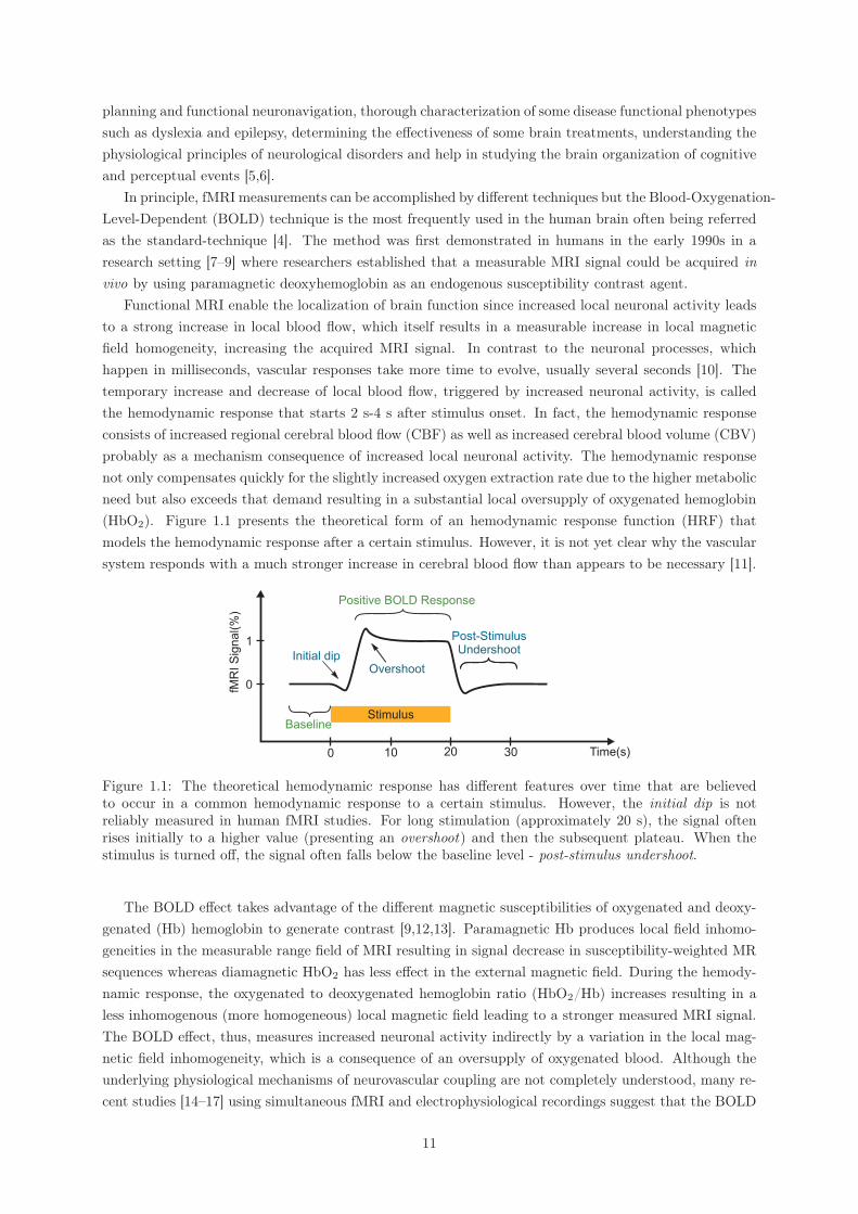
Functional MRI enable the localization of brain function since increased local neuronal activity leadsto a strong increase in local blood flow, which itself results in a measurable increase in local magneticfield homogeneity, increasing the acquired MRI signal. In contrast to the neuronal processes, whichhappen in milliseconds, vascular responses take more time to evolve, usually several seconds [10]. Thetemporary increase and decrease of local blood flow, triggered by increased neuronal activity, is calledthe hemodynamic response that starts 2 s-4 s after stimulus onset. In fact, the hemodynamic responseconsists of increased regional cerebral blood flow (CBF) as well as increased cerebral blood volume (CBV)probably as a mechanism consequence of increased local neuronal activity. The hemodynamic responsenot only compensates quickly for the slightly increased oxygen extraction rate due to the higher metabolicneed but also exceeds that demand resulting in a substantial local oversupply of oxygenated hemoglobin(HbO2). Figure 1.1 presents the theoretical form of an hemodynamic response function (HRF) thatmodels the hemodynamic response after a certain stimulus. However, it is not yet clear why the vascularsystem responds with a much stronger increase in cerebral blood flow than appears to be necessary [11].

Initial dipOvershoot

Post-StimulusUndershoot

Positive BOLD Response

Time(s)

fMR

IS

ign

al(%

)

StimulusBaseline

0 10 20 30

0

1

Figure 1.1: The theoretical hemodynamic response has different features over time that are believedto occur in a common hemodynamic response to a certain stimulus. However, the initial dip is notreliably measured in human fMRI studies. For long stimulation (approximately 20 s), the signal oftenrises initially to a higher value (presenting an overshoot) and then the subsequent plateau. When thestimulus is turned off, the signal often falls below the baseline level - post-stimulus undershoot.

The BOLD effect takes advantage of the different magnetic susceptibilities of oxygenated and deoxy-genated (Hb) hemoglobin to generate contrast [9,12,13]. Paramagnetic Hb produces local field inhomo-geneities in the measurable range field of MRI resulting in signal decrease in susceptibility-weighted MRsequences whereas diamagnetic HbO2 has less effect in the external magnetic field. During the hemody-namic response, the oxygenated to deoxygenated hemoglobin ratio (HbO2/Hb) increases resulting in aless inhomogenous (more homogeneous) local magnetic field leading to a stronger measured MRI signal.The BOLD effect, thus, measures increased neuronal activity indirectly by a variation in the local mag-netic field inhomogeneity, which is a consequence of an oversupply of oxygenated blood. Although theunderlying physiological mechanisms of neurovascular coupling are not completely understood, many re-cent studies [14–17] using simultaneous fMRI and electrophysiological recordings suggest that the BOLD

11

contrast mechanism directly reflects the neural responses elicited by a stimulus. So the change in localHbO2/Hb ratio and its associated change in the local magnetic field inhomogeneity acts as an endogenousmarker of neural activity.

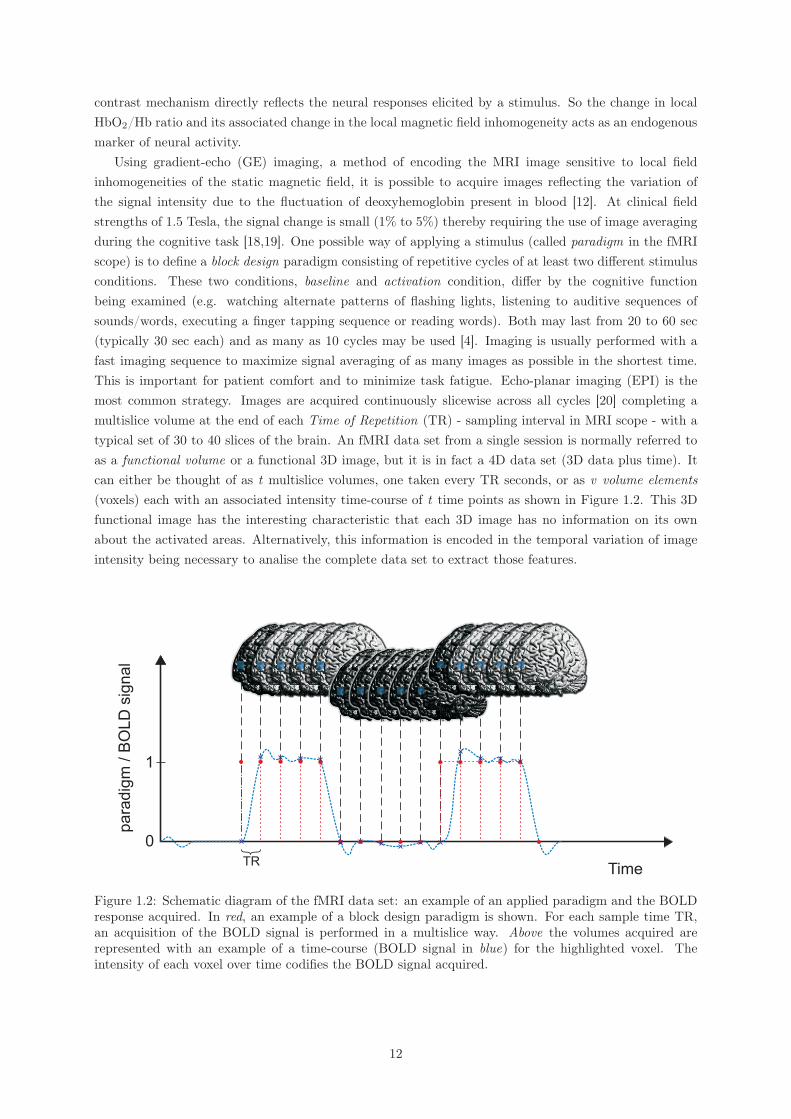
Using gradient-echo (GE) imaging, a method of encoding the MRI image sensitive to local fieldinhomogeneities of the static magnetic field, it is possible to acquire images reflecting the variation ofthe signal intensity due to the fluctuation of deoxyhemoglobin present in blood [12]. At clinical fieldstrengths of 1.5 Tesla, the signal change is small (1% to 5%) thereby requiring the use of image averagingduring the cognitive task [18,19]. One possible way of applying a stimulus (called paradigm in the fMRIscope) is to define a block design paradigm consisting of repetitive cycles of at least two different stimulusconditions. These two conditions, baseline and activation condition, differ by the cognitive functionbeing examined (e.g. watching alternate patterns of flashing lights, listening to auditive sequences ofsounds/words, executing a finger tapping sequence or reading words). Both may last from 20 to 60 sec(typically 30 sec each) and as many as 10 cycles may be used [4]. Imaging is usually performed with afast imaging sequence to maximize signal averaging of as many images as possible in the shortest time.This is important for patient comfort and to minimize task fatigue. Echo-planar imaging (EPI) is themost common strategy. Images are acquired continuously slicewise across all cycles [20] completing amultislice volume at the end of each Time of Repetition (TR) - sampling interval in MRI scope - with atypical set of 30 to 40 slices of the brain. An fMRI data set from a single session is normally referred toas a functional volume or a functional 3D image, but it is in fact a 4D data set (3D data plus time). Itcan either be thought of as t multislice volumes, one taken every TR seconds, or as v volume elements(voxels) each with an associated intensity time-course of t time points as shown in Figure 1.2. This 3Dfunctional image has the interesting characteristic that each 3D image has no information on its ownabout the activated areas. Alternatively, this information is encoded in the temporal variation of imageintensity being necessary to analise the complete data set to extract those features.

Time

para

dig

m/

BO

LD

sig

nal

0

1

TR

Figure 1.2: Schematic diagram of the fMRI data set: an example of an applied paradigm and the BOLDresponse acquired. In red, an example of a block design paradigm is shown. For each sample time TR,an acquisition of the BOLD signal is performed in a multislice way. Above the volumes acquired arerepresented with an example of a time-course (BOLD signal in blue) for the highlighted voxel. Theintensity of each voxel over time codifies the BOLD signal acquired.

12

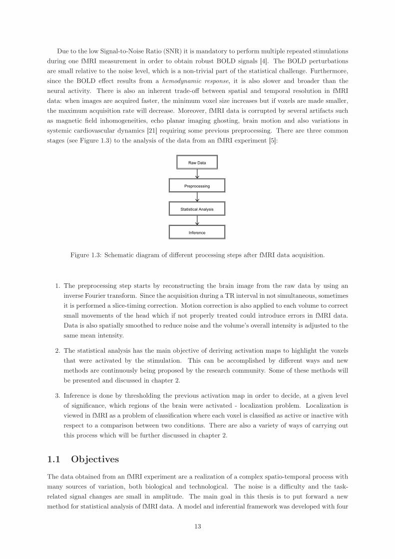
Due to the low Signal-to-Noise Ratio (SNR) it is mandatory to perform multiple repeated stimulationsduring one fMRI measurement in order to obtain robust BOLD signals [4]. The BOLD perturbationsare small relative to the noise level, which is a non-trivial part of the statistical challenge. Furthermore,since the BOLD effect results from a hemodynamic response, it is also slower and broader than theneural activity. There is also an inherent trade-off between spatial and temporal resolution in fMRIdata: when images are acquired faster, the minimum voxel size increases but if voxels are made smaller,the maximum acquisition rate will decrease. Moreover, fMRI data is corrupted by several artifacts suchas magnetic field inhomogeneities, echo planar imaging ghosting, brain motion and also variations insystemic cardiovascular dynamics [21] requiring some previous preprocessing. There are three commonstages (see Figure 1.3) to the analysis of the data from an fMRI experiment [5]:

Raw Data

Preprocessing

Statistical Analysis

Inference

Figure 1.3: Schematic diagram of different processing steps after fMRI data acquisition.

1. The preprocessing step starts by reconstructing the brain image from the raw data by using aninverse Fourier transform. Since the acquisition during a TR interval in not simultaneous, sometimesit is performed a slice-timing correction. Motion correction is also applied to each volume to correctsmall movements of the head which if not properly treated could introduce errors in fMRI data.Data is also spatially smoothed to reduce noise and the volume’s overall intensity is adjusted to thesame mean intensity.

2. The statistical analysis has the main objective of deriving activation maps to highlight the voxelsthat were activated by the stimulation. This can be accomplished by different ways and newmethods are continuously being proposed by the research community. Some of these methods willbe presented and discussed in chapter 2.

3. Inference is done by thresholding the previous activation map in order to decide, at a given levelof significance, which regions of the brain were activated - localization problem. Localization isviewed in fMRI as a problem of classification where each voxel is classified as active or inactive withrespect to a comparison between two conditions. There are also a variety of ways of carrying outthis process which will be further discussed in chapter 2.

1.1 Objectives

The data obtained from an fMRI experiment are a realization of a complex spatio-temporal process withmany sources of variation, both biological and technological. The noise is a difficulty and the task-related signal changes are small in amplitude. The main goal in this thesis is to put forward a newmethod for statistical analysis of fMRI data. A model and inferential framework was developed with four

13

key objectives of simultaneously detecting activated regions by an applied paradigm and estimating thehemodynamic response function of each voxel, introducing spatial information of the neighbouring pixelsto improve the detection and finally incorporating the usual preprocessing step of drift removal duringthe statistical analysis.

1.2 Original Contributions

Most of the work presented in this document is an original contribution to knowledge and has beenpublished or submitted:

• The first approach of simultaneously solving the activity detection problem and estimating thelocal HRF with the introduction of spatial correlation with the Graph Cuts algorithm (SPM-GC)was published at the 30th Annual International IEEE EMBS Conference in Vancouver, BritishColumbia, Canada ([22]);

• The SPM-GC algorithm was submitted as an extended abstract to the national conference RecPad2008 - 14a Conferência Portuguesa de Reconhecimento de Padrões;

• The last improvement of the SPM-GC algorithm with the important extension step of drift removalduring the statistical analysis (now called SPM-Drift-GC) was submitted to the Human BrainMapping international journal ([23]).

1.3 Thesis Organization

This thesis is organized as follows. Chapter 2 presents a brief literature review of the methods proposedin the main areas touching the present work of fMRI data analysis.

Chapter 3 formulates the problem and describes the developed approach to carry out the correctmodelling of the four key objectives described in 1.1.

Chapter 4 groups and discusses the main results obtained in testing several aspects of the proposedwork. Synthetic and Real Data was used to accomplish this.

Finally, chapter 5 concludes this thesis, discusses some limitations and suggests some possible futurework.

14

Chapter 2

Literature Review

In this chapter, a literature review of the three principal statistical challenges that are the main goal of thisthesis will be addressed. First, classical and Bayesian approach of modelling the functional neuroimagingdata are addressed. Second, methods to introduce spatial correlation in the estimation of coefficientsused to linearly combine the Explanatory Variables (EV) are described and finally, modelling of slowvariations drift in fMRI data are considered.

2.1 Classical and Bayesian Models

Statistical data analysis aims at making inference about underlying patterns in data that often containa large amount of random noise. This is the case of fMRI data. The usual approach is to construct amodel for the way in which the BOLD response depends on the stimulus. Such a model must includea component of random error which explains how the observations vary between different sessions evenif the conditions and the subject are the same. An example time course from a single voxel is shown inFig.2.1[5]. For some of the time points, stimulation was applied (the higher intensity periods), and atsome time points the subject was at rest. The effect of the stimulation is clear but the high frequencynoise is also present. The aim of fMRI analysis is to identify in which voxels’ time series the signal ofinterest is significantly greater than the noise level and presents an interdependence with the paradigmapplied. In the following two subsections, classical and Bayesian models will be addressed as ways ofsolving these problems.

But before describing those types of models it is important to distinguish between univariate statisticalmodels andmultivariate statistical models. Univariate models test each voxel’s time course independently.However, there are also multivariate methods which process all the data together. When individualobservations are not scalars, as in the case of fMRI in which observations are in the form of time courses,multivariate strategies are often the natural approach to statistical modelling. However, the most commonfMRI analysis is essentially a massively univariate approach, where identical univariate models are fittedat each voxel [24]. Since the method proposed in chapter 3 is essentially a univariate method with a finalstep of integration of spatial correlation, this thesis will focus the literature review mainly on this typeof analysis.

2.1.1 Classical Models

Functional mapping studies are classically analysed with statistical parametric mapping (SPM). Statis-tical parametric mapping requires the construction of continuous statistical processes to test hypothesisabout specific effects in regional cerebral activity [25]. SPM are images or fields with values that are

15

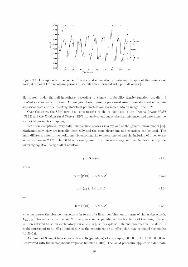
Figure 2.1: Example of a time course from a visual stimulation experiment. In spite of the presence ofnoise, it is possible to recognize periods of stimulation alternated with periods of rest[5].

distributed, under the null hypothesis, according to a known probability density function, usually a tStudent’s or an F -distribution. An analysis of each voxel is performed using these standard univariatestatistical tests and the resulting statistical parameters are assembled into an image - the SPM.

Over the years, the SPM term has come to refer to the conjoint use of the General Linear Model(GLM) and the Random Field Theory (RFT) to analyse and make classical inferences and determine thestatistical parametric mapping.

With few exceptions, every fMRI time course analysis is a variant of the general linear model [26].Mathematically, they are formally identically and the same algorithms and equations can be used. Themain difference rests in the design matrix encoding the temporal model and the inclusion of other termsas we will see in 2.1.2. The GLM is normally used in a univariate way and can be described by thefollowing equation using matrix notation

y = Xb + e (2.1)

where

y = {y(n)}, 1 ≤ n ≤ N, (2.2)

b = {βk}, 1 ≤ k ≤ L (2.3)

and

e = {ε(n)}, 1 ≤ n ≤ N (2.4)

which expresses the observed response y in terms of a linear combination of terms of the design matrix,X(N×L), plus an error term e for N time points and L paradigms. Each column of the design matrixis often referred to as an explanatory variable (EV), as it explains different processes in the data, itcould correspond to an effect applied during the experiment or an effect that may confound the results[10,26–28].

A column of X might be a series of 1s and 0s (paradigm) - for example, 0 0 0 0 0 1 1 1 1 1 0 0 0 0 0 etc- convolved with the hemodynamic response function (HRF). The GLM procedure applied to fMRI data

16

assumes a linear and time invariant (LTI) model [26]. This process of convolving the paradigm with theHRF mimics the effect that the brain’s neuro-physiology has on the input function (see Chapter 1). Thebrain’s hemodynamic response is a delayed and blurred version of the input stimulus, so the convolutionoperation is applied to the paradigm to create a delayed and blurred version of it, which will better fitthe data [5]. βk is an unknown or free parameter which characterises the effect of a particular stimulationcondition such as the one of the previous example and corresponds to the value that the square wave (ofheight 1) must be multiplied by to fit the correspondent square wave component in the data. The firststep of the GLM approach comprises of the estimation of the β parameters which will have a real value.For instance, if there are two types of stimuli, the model would be

y = β1x1 + β2x2 + ε. (2.5)

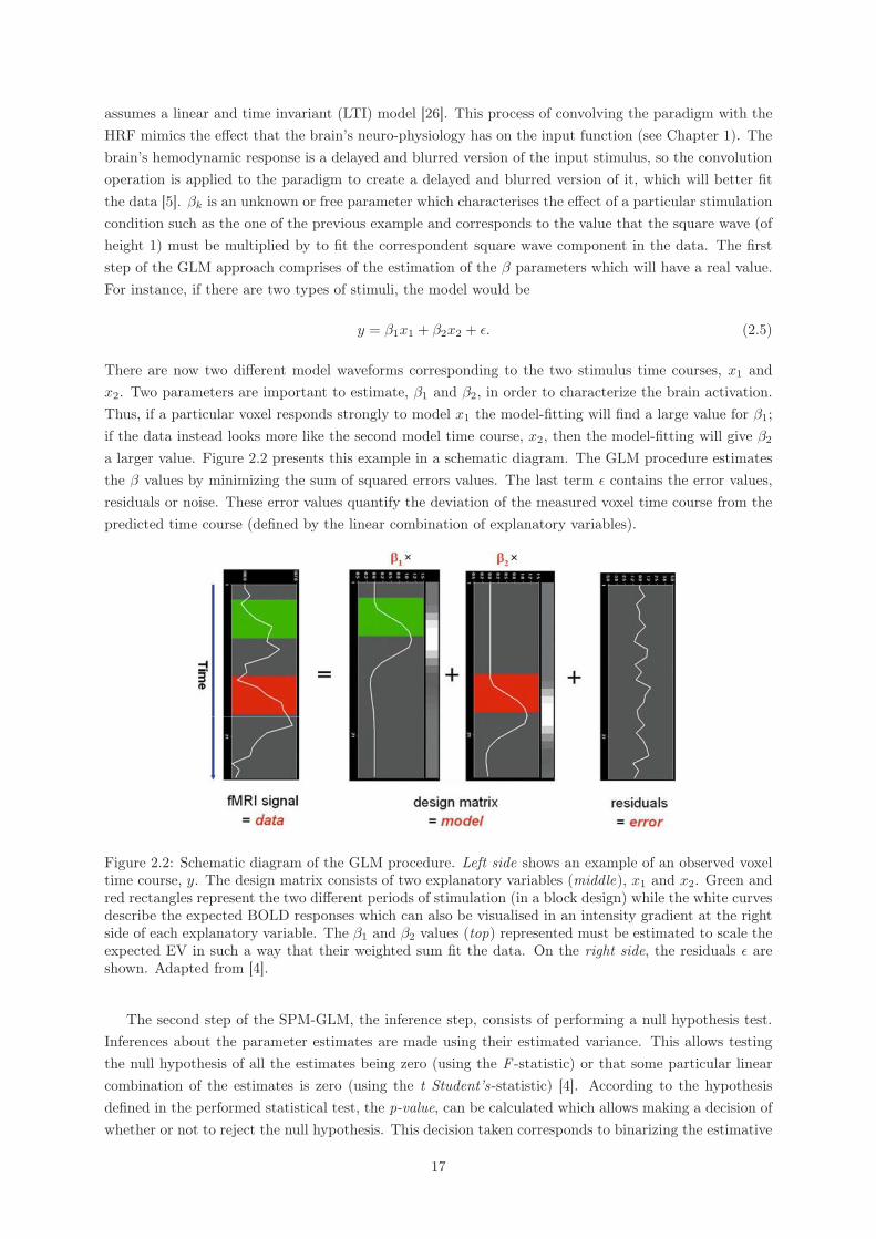
There are now two different model waveforms corresponding to the two stimulus time courses, x1 andx2. Two parameters are important to estimate, β1 and β2, in order to characterize the brain activation.Thus, if a particular voxel responds strongly to model x1 the model-fitting will find a large value for β1;if the data instead looks more like the second model time course, x2, then the model-fitting will give β2

a larger value. Figure 2.2 presents this example in a schematic diagram. The GLM procedure estimatesthe β values by minimizing the sum of squared errors values. The last term ε contains the error values,residuals or noise. These error values quantify the deviation of the measured voxel time course from thepredicted time course (defined by the linear combination of explanatory variables).

Figure 2.2: Schematic diagram of the GLM procedure. Left side shows an example of an observed voxeltime course, y. The design matrix consists of two explanatory variables (middle), x1 and x2. Green andred rectangles represent the two different periods of stimulation (in a block design) while the white curvesdescribe the expected BOLD responses which can also be visualised in an intensity gradient at the rightside of each explanatory variable. The β1 and β2 values (top) represented must be estimated to scale theexpected EV in such a way that their weighted sum fit the data. On the right side, the residuals ε areshown. Adapted from [4].

The second step of the SPM-GLM, the inference step, consists of performing a null hypothesis test.Inferences about the parameter estimates are made using their estimated variance. This allows testingthe null hypothesis of all the estimates being zero (using the F -statistic) or that some particular linearcombination of the estimates is zero (using the t Student’s-statistic) [4]. According to the hypothesisdefined in the performed statistical test, the p-value, can be calculated which allows making a decision ofwhether or not to reject the null hypothesis. This decision taken corresponds to binarizing the estimative

17

of the β value of each voxel that previously was a real value [5,29]. The usual confidence level generallyaccepted by the scientific community is 0.05 [4] so in the case of p-value< 0.05 the alternative hypothesismay be assumed and thus, the activation voxel is concluded.

The main drawback of this model is the huge number of tests being carried out, as much as the numberof voxels. The classical inference has a frequentist basis. So if 20 000 voxels are tested for a significanceof p < 0.01 then it is expected that 200 will be considered activate by chance, even if no stimulationis applied. It is not ideal to blindly accept these as being activated. This multiple-comparison problemmeans that it is not valid to accept all activations reported by this method; a correction is necessary toreduce the number of false positives. RFT is used to resolve the multiple comparison problem that arisesfrom making inferences over a whole volume [26]. This method takes into account the spatial smoothnessof the statistic map, i.e. estimates the number of statistically independent voxels, which is smaller thanthe original number [5].

Despite its success, statistical parametric mapping has several limitations [26,27,30] such as:

• The statistical parameter, the p-value, does not reflect the likelihood that the effect is present butsimply the probability of getting the observed data in the effect’s absence. As a consequence, we cannever reject the alternative hypothesis that an activation had not occured because the probabilitythat an effect is exactly zero is itself zero.

• Given that the probability of an effect being zero is rather small, one can always demonstrate asignificant effect at every voxel if enough scans are performed. This will increase the false positiverate. This can be problematic in cases of multiple subject statistics.

• Doing the correction to resolve the multiple comparison problem, the inference becomes sensitiveto the search volume being examined, i.e., the p-value change according to the number of voxelsthat one is classifying. The classical inference becomes less sensitive with large search volumes.However, the truth is that the probability that any voxel has been activated does not change withthe search volume.

All these problems would be avoided if instead of considering the likelihood of getting the data, givenno activation (classical approach), one considers the probability of a voxel’s activation higher than somethreshold. In fact, in the latter case, the multiple comparison problem does not have to be contendedbecause the probability that activation has occurred, given the data, at any particular voxel is the sameirrespective of whether one has analysed that voxel or the whole brain [30]. What one would really likeis the probability distribution of the activation given the data. This is the posterior probability used inBayesian inference [27].

2.1.2 Bayesian Models

The Bayesian approach is gaining popularity since it provides a formal method of incorporating priorknowledge in data analysis. Bayesian analysis regards the posterior probability, which summarises thedegree of one’s certainty concerning a given situation [31]. Bayesian models are based on conditionalinferences about an effect, given the data in opposition to the classical inference based on the data giventhe effect is zero.

Bayes’s law states that the posterior probability is proportional to the product of the likelihood andthe prior. The likelihood encompasses the information contained in the new data whereas the priorexpresses the degree of certainty about the situation before the data are taken. The Bayes’s law can bestated as

18

p(x|d) =

Likelihood︷ ︸︸ ︷p(d|x)

Prior︷︸︸︷p(x)

p(d)(2.6)

where x is a general parameter which one wishes to estimate and d is the data taken after an experiment.The probability p(x|d) is called the a posteriori probability density function or simply the posterior.The likelihood is usually derived from a model for predicting the data, given x (p(d|x)), as well as aprobabilistic model for the noise [32]. The term p(d) of equation (2.6) may be considered necessaryonly for normalization purposes being many times discarded and giving rise to Bayes’s law written as aproportionality of the likelihood and the prior terms. Another equivalent formulation corresponds to themaximization of the joint probability function which can be written as p(d, x) = p(d|x)p(x), for p(x) �= 0.

In some situations the data alone may not be sufficient to specify a unique solution to the problemin analysis, which leads to an ill-posed problem [33]. The prior term introduced by the Bayesian methodcan help in guiding the result towards a preferred solution. So Bayesian estimation is naturally biasedto the prior information used and can be regarded as enforcing soft constraints on parameter values [24].Furthermore, the Bayesian method provides a coherent approach for statistical analysis, of which theclassical framework can be seen as a particular case [34]. With increasing number of observations, theprior becomes less important and hence the Bayesian result will converge to the likelihood-only frequentistresult.

In one interpretation of Bayes’s law, the prior stands for knowledge acquired in a previous experimentbeing estimated from the data - empirical Bayes [27]. In another interpretation, the prior might introduceadditional information about the parameter x. The prior works as a way to restrict x so that the posteriorprovides more information about x than only the one introduced by the likelihood. In fact, many differentpriors might be chosen in the Bayesian analysis depending on the domain of the problem, the type ofdata and the model employed.

Marrelec et al [35] present a Bayesian non-parametric estimation of the HRF. The authors make useof temporal prior terms to introduce physiological knowledge about the HRF. Basic and soft constraintswere incorporate in the Bayesian analysis performed namely considering that the HRF starts and endsat zero and the HRF is a smooth function. The former was achieved by setting the first and last samplepoints of the HRF to zero. The latter was accomplished by setting a Gaussian prior for the norm ofthe second derivative of the HRF. The relative weight of the prior to the HRF estimative was adjustedby an hyperparameter playing the role of a regularization parameter. Using this approach, the authorsdemonstrate an increase in the performance by using these prior terms when compared to the classicalMaximum-Likelihood estimator.

Another Bayesian approach based on the general mathematical formalism of the GLM is proposedby Afonso et al [36]. The authors describe a Bayesian Statistical Parametric Mapping algorithm basedon the maximum a posteriori (MAP) criterion to jointly estimate and detect the activated brain areascharacterised by the β coefficients, assumed to be binary variables. The prior term introduced for theseparameters comprises a bimodal distribution defined as the sum of two Gaussian distributions centeredat zero and one. The authors show that the introduction of this prior term improves the estimation ofthe β coefficients that characterise the activation brain maps.

2.2 Modelling Spatial Correlation

Introducing information from the neighbouring voxels when classifying a specific voxel could reduce thenumber of activation errors. In fact, it is well known that each neuron of the cerebrum makes synaptic

19

contact with thousands of other neurons and it never occurs that a single neuron is provoked into activityas the result of signals from just one other neuron [37]. These brain networks are translated into activatedregions when an fMRI experiment is performed. An important feature of fMRI data described in theliterature is its tendency toward clustered activation. It is reported that true neural activity tends tostimulate signal changes over contiguous groups of voxels [38]. So using this information, one can saythat it is less probable that non-activated voxels appear inside of an activated region and the conversealso applies. Incorporating this knowledge during statistical analysis will avoid misclassification insideactivated regions.

A frequently referred approach that addresses nonindependence between voxels corresponds to ini-tially smoothing the data, performing an univariate statistical analysis and applying RFT to decide thesignificance of the obtained set of voxels [39].

In [40] a method of introducing contextual information is proposed based on Markov Random Fieldsin a Bayesian framework. Using this method, a voxel will be classified according to its intensity levelbut also with respect to the value of its neighbours. The dependency between neighbouring voxels ismodelled by local interactions. Those interactions together lead to a global energy which is minimizedusing simulated annealing [41].

In [42] a spatio-temporal regression analysis addressing spatial correlation information is described.Each voxel has a regression model including its time course and the time course from the neighbouringvoxels. The intrinsic temporal and spatial correlation structures are modeled together using a separablemodel.

2.3 Modelling Slow Variation Drift

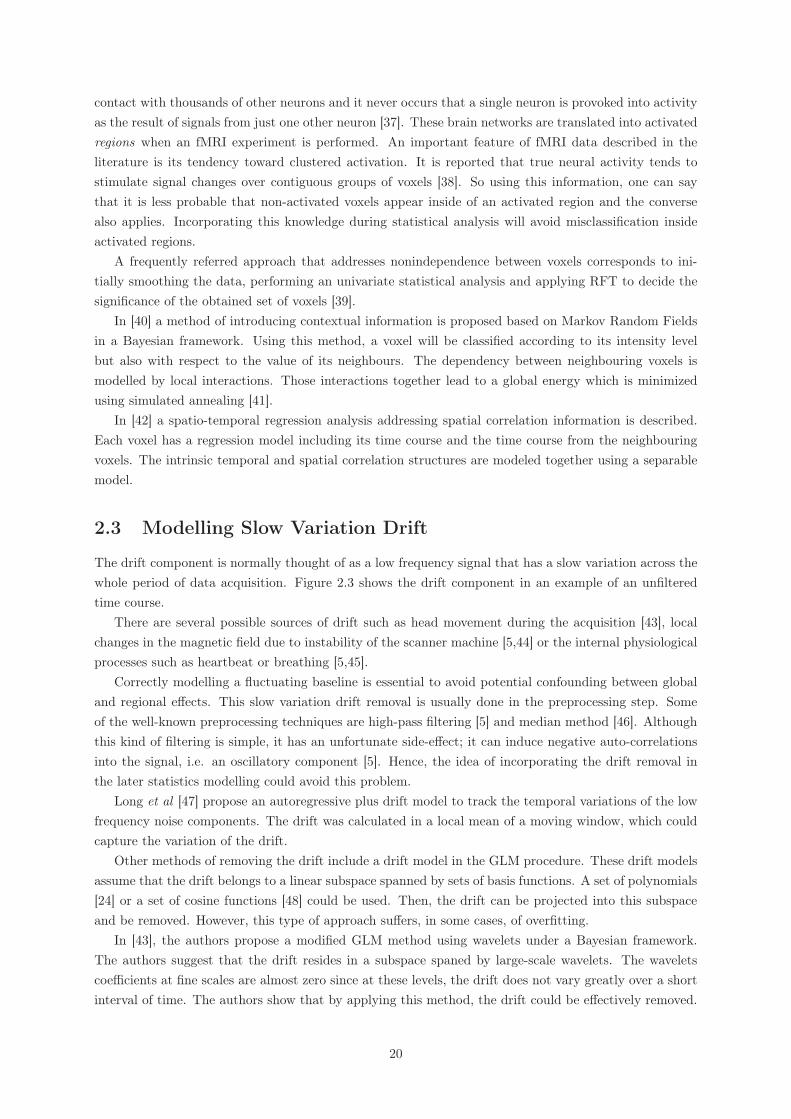
The drift component is normally thought of as a low frequency signal that has a slow variation across thewhole period of data acquisition. Figure 2.3 shows the drift component in an example of an unfilteredtime course.

There are several possible sources of drift such as head movement during the acquisition [43], localchanges in the magnetic field due to instability of the scanner machine [5,44] or the internal physiologicalprocesses such as heartbeat or breathing [5,45].

Correctly modelling a fluctuating baseline is essential to avoid potential confounding between globaland regional effects. This slow variation drift removal is usually done in the preprocessing step. Someof the well-known preprocessing techniques are high-pass filtering [5] and median method [46]. Althoughthis kind of filtering is simple, it has an unfortunate side-effect; it can induce negative auto-correlationsinto the signal, i.e. an oscillatory component [5]. Hence, the idea of incorporating the drift removal inthe later statistics modelling could avoid this problem.

Long et al [47] propose an autoregressive plus drift model to track the temporal variations of the lowfrequency noise components. The drift was calculated in a local mean of a moving window, which couldcapture the variation of the drift.

Other methods of removing the drift include a drift model in the GLM procedure. These drift modelsassume that the drift belongs to a linear subspace spanned by sets of basis functions. A set of polynomials[24] or a set of cosine functions [48] could be used. Then, the drift can be projected into this subspaceand be removed. However, this type of approach suffers, in some cases, of overfitting.

In [43], the authors propose a modified GLM method using wavelets under a Bayesian framework.The authors suggest that the drift resides in a subspace spaned by large-scale wavelets. The waveletscoefficients at fine scales are almost zero since at these levels, the drift does not vary greatly over a shortinterval of time. The authors show that by applying this method, the drift could be effectively removed.

20

Unfiltered Time-Course

Drift Component

High Frequency NoiseHigh-Frequency Noise

Signal of Interest

Figure 2.3: Schematic representation of an unfiltered time course from an activated voxel and its de-composition. Top: Unfiltered time course. Upper Middle: Representation of the Drift Componentcorrespondent to the Low frequency noise. Lower Middle: Representation of the High frequency noise.Bottom: Signal of interest. Adapted from [5].

21

Chapter 3

Proposed Method

The present work comprises the introduction of a new analysis method (henceforth, referred to as SPM-Drift-GC) that combines the brain activity detection problem, the local hemodynamic response charac-terisation by estimating the local HRF and also includes the removal of the low frequency signal (drift)commonly present in the fMRI data. The inclusion of a final step that introduces spatial correlation tothe data analysis performed using the Graph Cuts algorithm [49] brings remarkable improvements in theaccuracy of activity detection as shown in the results presented in chapter 4.

3.1 Notation

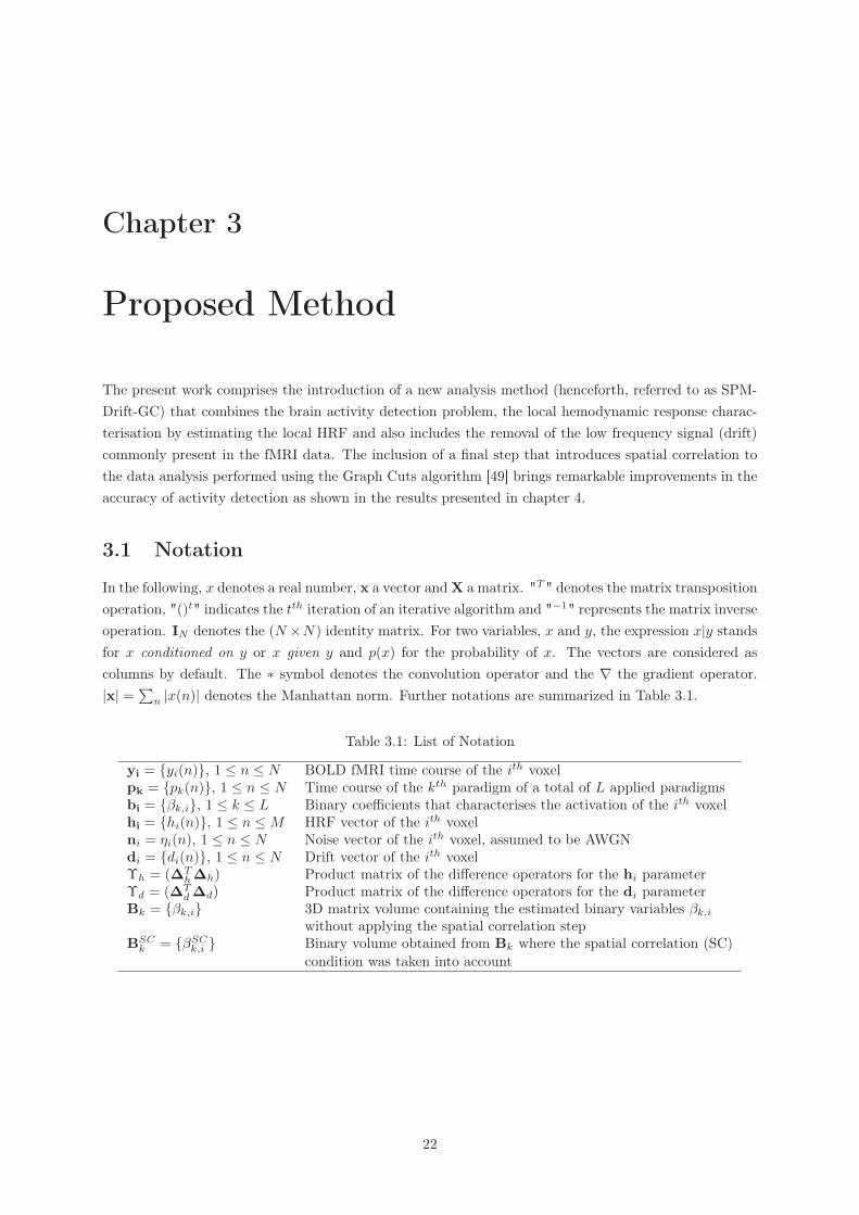
In the following, x denotes a real number, x a vector and X a matrix. "T " denotes the matrix transpositionoperation, "()t" indicates the tth iteration of an iterative algorithm and "−1" represents the matrix inverseoperation. IN denotes the (N ×N) identity matrix. For two variables, x and y, the expression x|y standsfor x conditioned on y or x given y and p(x) for the probability of x. The vectors are considered ascolumns by default. The ∗ symbol denotes the convolution operator and the ∇ the gradient operator.|x| = ∑

n |x(n)| denotes the Manhattan norm. Further notations are summarized in Table 3.1.

Table 3.1: List of Notation

yi = {yi(n)}, 1 ≤ n ≤ N BOLD fMRI time course of the ith voxelpk = {pk(n)}, 1 ≤ n ≤ N Time course of the kth paradigm of a total of L applied paradigmsbi = {βk,i}, 1 ≤ k ≤ L Binary coefficients that characterises the activation of the ith voxelhi = {hi(n)}, 1 ≤ n ≤ M HRF vector of the ith voxelni = ηi(n), 1 ≤ n ≤ N Noise vector of the ith voxel, assumed to be AWGNdi = {di(n)}, 1 ≤ n ≤ N Drift vector of the ith voxelΥh = (ΔT

h Δh) Product matrix of the difference operators for the hi parameterΥd = (ΔT

d Δd) Product matrix of the difference operators for the di parameterBk = {βk,i} 3D matrix volume containing the estimated binary variables βk,i

without applying the spatial correlation stepBSC

k = {βSCk,i } Binary volume obtained from Bk where the spatial correlation (SC)

condition was taken into account

22

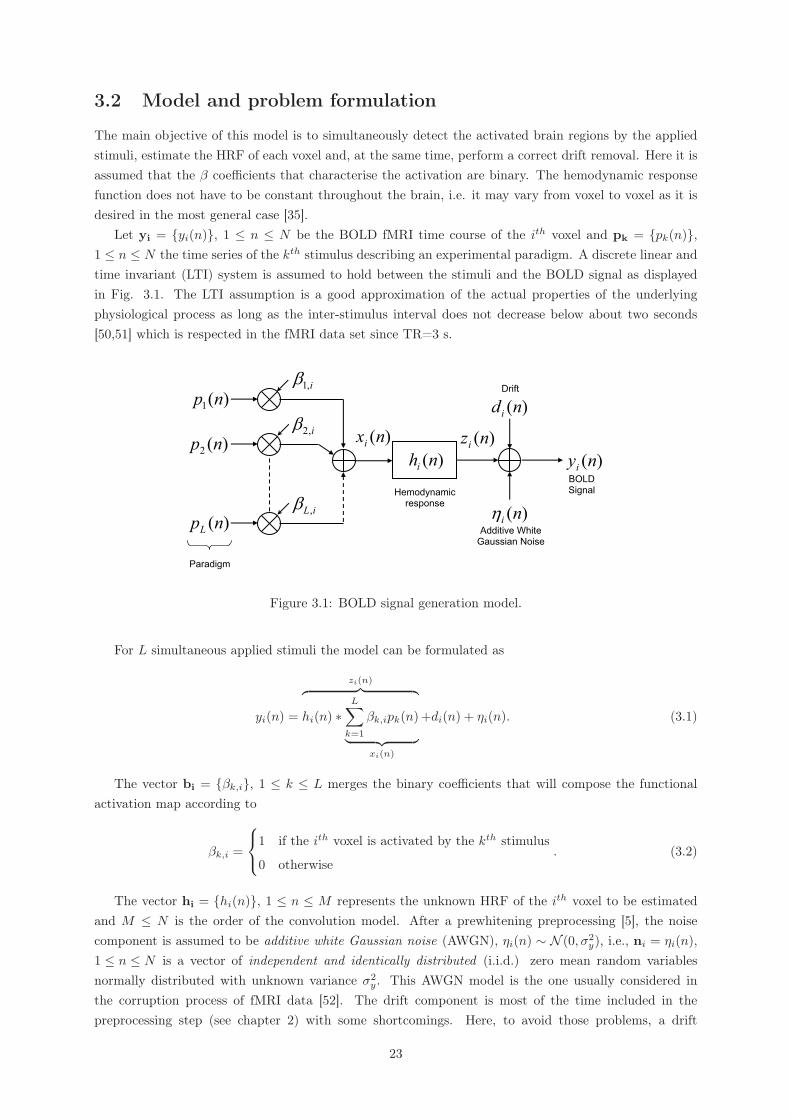
3.2 Model and problem formulation

The main objective of this model is to simultaneously detect the activated brain regions by the appliedstimuli, estimate the HRF of each voxel and, at the same time, perform a correct drift removal. Here it isassumed that the β coefficients that characterise the activation are binary. The hemodynamic responsefunction does not have to be constant throughout the brain, i.e. it may vary from voxel to voxel as it isdesired in the most general case [35].

Let yi = {yi(n)}, 1 ≤ n ≤ N be the BOLD fMRI time course of the ith voxel and pk = {pk(n)},1 ≤ n ≤ N the time series of the kth stimulus describing an experimental paradigm. A discrete linear andtime invariant (LTI) system is assumed to hold between the stimuli and the BOLD signal as displayedin Fig. 3.1. The LTI assumption is a good approximation of the actual properties of the underlyingphysiological process as long as the inter-stimulus interval does not decrease below about two seconds[50,51] which is respected in the fMRI data set since TR=3 s.

)(1 np

)(2 np

)(npL

i,1�

i,2�

iL,�

)(nxi )(nzi)(nyi)(nhi

Hemodynamicresponse

)(ni�Additive White

Gaussian Noise

BOLDSignal

Paradigm

)(ndiDrift

Figure 3.1: BOLD signal generation model.

For L simultaneous applied stimuli the model can be formulated as

yi(n) =

zi(n)︷ ︸︸ ︷hi(n) ∗

L∑k=1

βk,ipk(n)

︸ ︷︷ ︸xi(n)

+di(n) + ηi(n). (3.1)

The vector bi = {βk,i}, 1 ≤ k ≤ L merges the binary coefficients that will compose the functionalactivation map according to

βk,i =

⎧⎨⎩

1 if the ith voxel is activated by the kth stimulus

0 otherwise. (3.2)

The vector hi = {hi(n)}, 1 ≤ n ≤ M represents the unknown HRF of the ith voxel to be estimatedand M ≤ N is the order of the convolution model. After a prewhitening preprocessing [5], the noisecomponent is assumed to be additive white Gaussian noise (AWGN), ηi(n) ∼ N (0, σ2

y), i.e., ni = ηi(n),1 ≤ n ≤ N is a vector of independent and identically distributed (i.i.d.) zero mean random variablesnormally distributed with unknown variance σ2

y. This AWGN model is the one usually considered inthe corruption process of fMRI data [52]. The drift component is most of the time included in thepreprocessing step (see chapter 2) with some shortcomings. Here, to avoid those problems, a drift

23

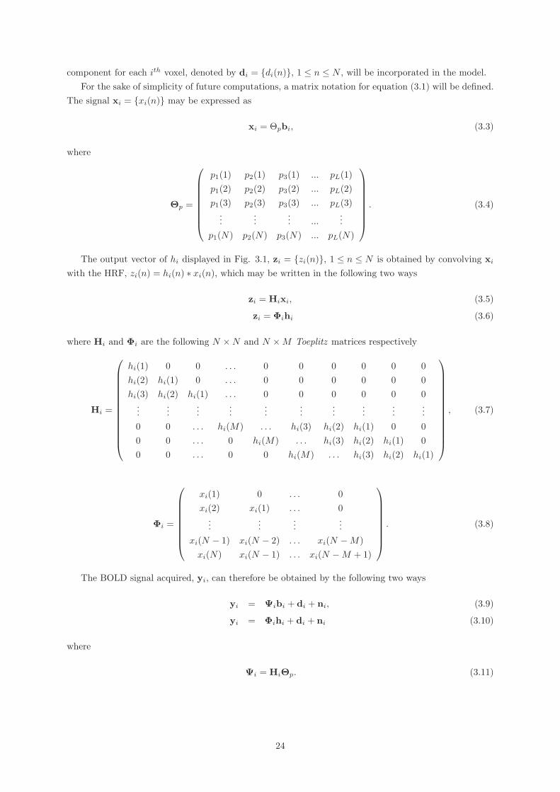
component for each ith voxel, denoted by di = {di(n)}, 1 ≤ n ≤ N , will be incorporated in the model.For the sake of simplicity of future computations, a matrix notation for equation (3.1) will be defined.

The signal xi = {xi(n)} may be expressed as

xi = Θpbi, (3.3)

where

Θp =

⎛⎜⎜⎜⎜⎜⎜⎜⎝

p1(1) p2(1) p3(1) ... pL(1)p1(2) p2(2) p3(2) ... pL(2)p1(3) p2(3) p3(3) ... pL(3)

......

... ......

p1(N) p2(N) p3(N) ... pL(N)

⎞⎟⎟⎟⎟⎟⎟⎟⎠

. (3.4)

The output vector of hi displayed in Fig. 3.1, zi = {zi(n)}, 1 ≤ n ≤ N is obtained by convolving xi

with the HRF, zi(n) = hi(n) ∗ xi(n), which may be written in the following two ways

zi = Hixi, (3.5)

zi = Φihi (3.6)

where Hi and Φi are the following N ×N and N ×M Toeplitz matrices respectively

Hi =

⎛⎜⎜⎜⎜⎜⎜⎜⎜⎜⎜⎜⎜⎝

hi(1) 0 0 . . . 0 0 0 0 0 0hi(2) hi(1) 0 . . . 0 0 0 0 0 0hi(3) hi(2) hi(1) . . . 0 0 0 0 0 0

......

......

......

......

......

0 0 . . . hi(M) . . . hi(3) hi(2) hi(1) 0 00 0 . . . 0 hi(M) . . . hi(3) hi(2) hi(1) 00 0 . . . 0 0 hi(M) . . . hi(3) hi(2) hi(1)

⎞⎟⎟⎟⎟⎟⎟⎟⎟⎟⎟⎟⎟⎠

, (3.7)

Φi =

⎛⎜⎜⎜⎜⎜⎜⎜⎝

xi(1) 0 . . . 0xi(2) xi(1) . . . 0

......

......

xi(N − 1) xi(N − 2) . . . xi(N −M)xi(N) xi(N − 1) . . . xi(N −M + 1)

⎞⎟⎟⎟⎟⎟⎟⎟⎠

. (3.8)

The BOLD signal acquired, yi, can therefore be obtained by the following two ways

yi = Ψibi + di + ni, (3.9)

yi = Φihi + di + ni (3.10)

where

Ψi = HiΘp. (3.11)

24

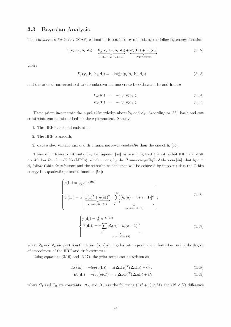
3.3 Bayesian Analysis

The Maximum a Posteriori (MAP) estimation is obtained by minimizing the following energy function

E(yi,bi,hi,di) = Ey(yi,bi,hi,di)︸ ︷︷ ︸Data fidelity term

+Eh(hi) + Ed(di)︸ ︷︷ ︸Prior terms

(3.12)

where

Ey(yi,bi,hi,di) = − log(p(yi|bi,hi,di)) (3.13)

and the prior terms associated to the unknown parameters to be estimated, bi and hi, are

Eh(hi) = − log(p(hi)), (3.14)

Ed(di) = − log(p(di)). (3.15)

These priors incorporate the a priori knowledge about hi and di. According to [35], basic and softconstraints can be established for these parameters. Namely,

1. The HRF starts and ends at 0;

2. The HRF is smooth;

3. di is a slow varying signal with a much narrower bandwidth than the one of hi [53].

These smoothness constraints may be imposed [54] by assuming that the estimated HRF and driftare Markov Random Fields (MRFs), which means, by the Hammersley-Clifford theorem [55], that hi anddi follow Gibbs distributions and the smoothness condition will be achieved by imposing that the Gibbsenergy is a quadratic potential function [54]:

⎧⎪⎪⎪⎪⎪⎪⎪⎨⎪⎪⎪⎪⎪⎪⎪⎩

p(hi) = 1Zh

e−U(hi)

U(hi) = α

⎡⎢⎢⎢⎢⎣h(1)2 + h(M)2︸ ︷︷ ︸

constraint (1)

+M∑

n=2

[hi(n)− hi(n− 1)]2

︸ ︷︷ ︸constraint (2)

⎤⎥⎥⎥⎥⎦ ,

(3.16)

⎧⎪⎪⎪⎪⎨⎪⎪⎪⎪⎩

p(di) = 1Zd

e−U(di)

U(di)i = γ∑

n

[di(n)− di(n− 1)]2

︸ ︷︷ ︸constraint (3)

(3.17)

where Zh and Zd are partition functions, [α, γ] are regularization parameters that allow tuning the degreeof smoothness of the HRF and drift estimates.

Using equations (3.16) and (3.17), the prior terms can be written as

Eh(hi) = −log(p(h)) = α(Δhhi)T (Δhhi) + C1, (3.18)

Ed(di) = −log(p(d)) = γ(Δddi)T (Δddi) + C2 (3.19)

where C1 and C2 are constants. Δh and Δd are the following ((M + 1) ×M) and (N × N) difference

25

operators, respectively:

Δh =

⎛⎜⎜⎜⎜⎜⎜⎜⎜⎜⎝

1 0 0 ... 0 0−1 1 0 ... 0 00 −1 1 ... 0 0...

......

. . . 0 00 0 0 ... −1 10 0 0 ... 0 1

⎞⎟⎟⎟⎟⎟⎟⎟⎟⎟⎠

, (3.20)

Δd =

⎛⎜⎜⎜⎜⎜⎜⎜⎝

1 −1 0 ... 0 0−1 1 0 ... 0 00 −1 1 ... 0 0...

......

. . . 0 00 0 0 ... −1 1

⎞⎟⎟⎟⎟⎟⎟⎟⎠

. (3.21)

The MAP estimation is performed by computing for each parameter the

∇E(yi,bi,hi,di) = 0. (3.22)

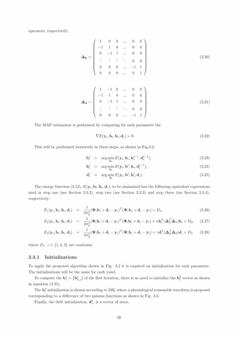
This will be performed iteratively in three steps, as shown in Fig.3.2,

bti = arg min

bi

E(yi,bi,ht−1i ,dt−1

i ), (3.23)

hti = arg min

hi

E(yi,bt,hi,dt−1i ), (3.24)

dti = arg min

di

E(yi,bt,hti,di). (3.25)

The energy function (3.12), E(yi,bi,hi,di), to be minimized has the following equivalent expressionsused in step one (see Section 3.3.2), step two (see Section 3.3.3) and step three (see Section 3.3.4),respectively:

E1(yi,bi,hi,di) =1

2σ2y

(Ψibi + di − yi)T (Ψibi + di − yi) + D1, (3.26)

E2(yi,bi,hi,di) =1

2σ2y

(Φihi + di − yi)T (Φihi + di − yi) + αhTi (ΔT

h Δh)hi + D2, (3.27)

E3(yi,bi,hi,di) =1

2σ2y

(Ψibi + di − yi)T (Ψibi + di − yi) + γdTi (ΔT

d Δd)di + D3 (3.28)

where Dr, r ∈ {1, 2, 3} are constants.

3.3.1 Initializations

To apply the proposed algorithm shown in Fig. 3.2 it is required an initialization for each parameter.The initializations will be the same for each voxel.

To compute the b1i = {b1

k,i} of the first iteration, there is no need to initialize the b0i vector as shown

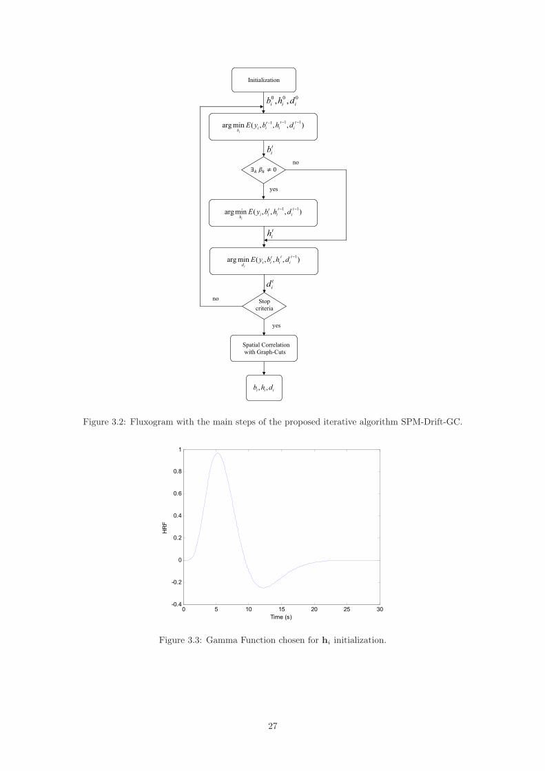
in equation (3.31).The h0

i initialization is chosen according to [56], where a physiological reasonable waveform is proposedcorresponding to a difference of two gamma functions as shown in Fig. 3.3.

Finally, the drift initialization, d0i , is a vector of zeros.

26

Spatial Correlation with Graph-Cuts

no

),,,(minarg 111 ti

ti

tiib

dhbyEi

iii dhb ,,

tih

Stopcriteria

),,,(minarg 11 ti

ti

tiih

dhbyEi

),,,(minarg 1ti

ti

tiid

dhbyEi

tid

no

yes

Initialization

000 ,, iii dhb

tib

yes

Figure 3.2: Fluxogram with the main steps of the proposed iterative algorithm SPM-Drift-GC.

0 5 10 15 20 25 30-0.4

-0.2

0

0.2

0.4

0.6

0.8

1

Time (s)

HR

F

Figure 3.3: Gamma Function chosen for hi initialization.

27

3.3.2 Step One: b estimation

The estimation of bi is achieved by minimizing the energy function (3.26) which may be written as follows

E1(yi,bi,hi,di) =1

2σ2y

L∑k=1

N∑n=1

(Ψi(n, k)βk,i + di(n)− yi(n))2 + D1 (3.29)

where each k term is

N∑n=1

(Ψi(n, k)βk,i + di(n)− yi(n))2 =

⎧⎨⎩

∑Nn=1(yi(n)− di(n))2 , βk,i = 0∑Nn=1(Ψi(n, k) + di(n)− yi(n))2 , βk,i = 1

. (3.30)

Therefore, the estimation of βk,i that leads to the minimization of (3.26) is the following

βk,i =

⎧⎨⎩

1 if∑

n

[Ψ2

i (n, k) + 2Ψi(n, k)(di(n)− yi(n))] ≤ 0

0 otherwise. (3.31)

3.3.3 Step Two: h estimation

In the second step, a new estimative of hi is calculated by solving the following equation

∇E2(yi,bi,hi,di) = ΦTi (Φihi + di − yi) + 2ασ2

yΥTh hi = 0 (3.32)

where Υh = (ΔTh Δh) is defined to simplify the expression. The solution of (3.32) is

hi =[ΦT

i Φi + 2ασ2yΥT

h

]−1ΦT

i (yi − di) (3.33)

where Φi = Φi(xi(bi)) is calculated using the bi estimation, bi, obtained in the previous step (see Section3.3.2). However, the HRF is only estimated in the case of voxel activation by at least one paradigm asshown in Fig. 3.2. In these cases, the HRF estimation may provide a useful insight about the local BOLDdynamics.

3.3.4 Step Three: d estimation

In this step, the slow variation drift, di, is estimated by solving

∇E3(yi,bi,hi,di) = (Ψibi + di − yi) + 2γσ2yΥT

d di = 0 (3.34)

where Υd = (ΔTd Δd) is defined to simplify the expression. The solution of (3.34) is

di =[IN + 2γσ2

yΥTh

]−1(yi −Ψibi) (3.35)

where Ψi = Ψi(hi) is calculated using the hi estimation, hi, obtained in the previous step (see Section3.3.3) and the bi vector will be substituted by bi, the estimation obtained in the first step (see Section3.3.2).

Since γ is a regularization parameter of a drift signal, a much slower frequency signal than HRF, thenγ should be much higher than α, i.e., γ � α [53].

28

3.3.5 Step Four: Spatial Correlation

This final step introduced here is performed independently for each k stimulus by using the algorithmproposed in [49] where spatial correlation is introduced. In fact, this is the only step where the correlationamong neighbours is considered as the previous estimation procedure of bi, hi and di was performedindependently of the neighbours’ voxels on a time course basis.

Let Bk = {βk,i} be a 3D matrix volume containing the estimated binary variables βk,i of the kth

stimulus for each i voxel (see section 3.3.2), where 1 ≤ i ≤ Ω being Ω = S × N ×M with S being thetotal number of slices, each containing N ×M voxels. Let also define BSC

k = {βSCk,i } as a binary volume

obtained from Bk, where the spatial correlation (SC) condition was taken into account by estimating

BSCk = arg min

BSCk

E4(Bk,BSCk ). (3.36)

The energy function is

E4(Bk,BSCk ) =

data term︷ ︸︸ ︷∑i

|βSCk,i − βk,i| (3.37)

+ λ∑

i

[V (βSC

k,i , βSCk,ih

) + V (βSCk,i , βSC

k,iv))

]/gi

︸ ︷︷ ︸regularization term

where βSCk,ih

and βSCk,iv

are the horizontal and vertical causal neighbours of βSCk,i at each slice, λ is a

parameter to tune the strength of smoothness, gi (ε ≤ gi ≤ 1) is the normalized gradient of Bk at theith node and ε = 10−2 is a small number to avoid division by zero. V (β1, β2) is a penalization functiondefined as follows

V (β1, β2) =

⎧⎨⎩

0 β1 = β2

1 β1 �= β2

. (3.38)

The energy function (3.37) is composed by two terms. The first forces the classification to be βSCk,i =

βk,i by minimizing the sum of absolute differences. The second term forces the uniformity of the solutionbecause the cost associated with uniform labels is smaller than non uniform ones (see equation (3.38)).However, in order to preserve transitions, the second term also includes a division by the normalizedsmoothed gradient magnitude of βk,i at ith location, gi. Therefore, when the gradient magnitude increases,the regularization strength is reduced at that location.

The minimization task of (3.37), formulated in (3.36), is a huge combinatorial optimization problemin the {0, 1}Ω high dimensional space where Ω is the number of voxels in each 3D volume.

In [49], it is shown that several energy minimization problems in high dimensional discrete spacescan be efficiently solved by using Graph Cuts (GC) based algorithms. The authors have designed a veryfast and efficient algorithm to compute the global minimum of the energy function based on graph cuts(minimum cut/maximum flow method). These kind of algorithms have different possible applicationsnamely, in computer vision, image restoration [57] but also in dynamic medical data [58]. However, thealgorithm is not completely general which means that some energy functions can not be minimized withthis method. In [57], the authors present a wide class of energy functions that may be minimized withthe GC method and the function (3.37) belongs to that class.

29

The four steps-algorithm is summarized in Table 3.2.

Table 3.2: Prototype algorithm

1. � Initialization,

2. � set iteration t = 1,

3. � set i = 1,

4. � set k = 1,

5. � estimate bi according to (3.31),

6. � estimate hi according to (3.33),

7. � estimate di according to (3.35),

8. � increment k and return to step 5 if k < L,

9. � increment i and return to step 4 if i < total number of voxels,

10. � increment t and return to step 3 while∑

i |bti − bt−1

i | �= 0 ,

11. � estimate βSCk,i from βk,i for all voxels taking into account spatial

correlation by using the Graph Cuts algorithm.

30

Chapter 4

Experimental Results

To evaluate the performance of the complete proposed method, Monte Carlo tests were performed usingsynthetic data (see Section 4.1) with increasing noise levels corruption. Real data was also analysedusing the SPM-Drift-GC algorithm and a comparison with the results provided by a neurologist usingthe BrainVoyager [59] software was done to validate the proposed method (see Section 4.2).

4.1 Synthetic Data

4.1.1 Brain Activation Detection

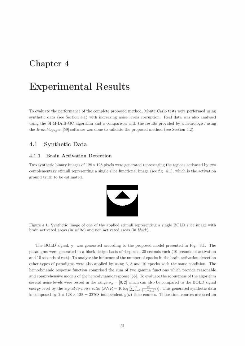
Two synthetic binary images of 128×128 pixels were generated representing the regions activated by twocomplementary stimuli representing a single slice functional image (see fig. 4.1), which is the activationground truth to be estimated.

Figure 4.1: Synthetic image of one of the applied stimuli representing a single BOLD slice image withbrain activated areas (in white) and non activated areas (in black).

The BOLD signal, y, was generated according to the proposed model presented in Fig. 3.1. Theparadigms were generated in a block-design basis of 4 epochs, 20 seconds each (10 seconds of activationand 10 seconds of rest). To analyse the influence of the number of epochs in the brain activation detectionother types of paradigms were also applied by using 6, 8 and 10 epochs with the same condition. Thehemodynamic response function comprised the sum of two gamma functions which provide reasonableand comprehensive models of the hemodynamic response [56]. To evaluate the robustness of the algorithmseveral noise levels were tested in the range σy = [0; 2] which can also be compared to the BOLD signalenergy level by the signal-to-noise ratio (SNR = 10 log(

∑Nn=1

z2n

(zn−yn)2 )). This generated synthetic datais composed by 2 × 128 × 128 = 32768 independent y(n) time courses. These time courses are used on

31

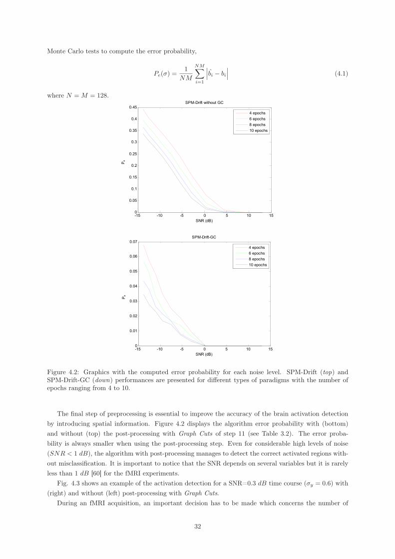
Monte Carlo tests to compute the error probability,

Pe(σ) =1

NM

NM∑i=1

∣∣∣bi − bi

∣∣∣ (4.1)

where N = M = 128.

-15 -10 -5 0 5 10 150

0.05

0.1

0.15

0.2

0.25

0.3

0.35

0.4

0.45

SNR (dB)

SPM-Drift without GC

4 epochs6 epochs8 epochs10 epochs

-15 -10 -5 0 5 10 150

0.01

0.02

0.03

0.04

0.05

0.06

0.07

SNR (dB)

SPM-Drift-GC

4 epochs6 epochs8 epochs10 epochs

Pe

Pe

Figure 4.2: Graphics with the computed error probability for each noise level. SPM-Drift (top) andSPM-Drift-GC (down) performances are presented for different types of paradigms with the number ofepochs ranging from 4 to 10.

The final step of preprocessing is essential to improve the accuracy of the brain activation detectionby introducing spatial information. Figure 4.2 displays the algorithm error probability with (bottom)and without (top) the post-processing with Graph Cuts of step 11 (see Table 3.2). The error proba-bility is always smaller when using the post-processing step. Even for considerable high levels of noise(SNR < 1 dB), the algorithm with post-processing manages to detect the correct activated regions with-out misclassification. It is important to notice that the SNR depends on several variables but it is rarelyless than 1 dB [60] for the fMRI experiments.

Fig. 4.3 shows an example of the activation detection for a SNR=0.3 dB time course (σy = 0.6) with(right) and without (left) post-processing with Graph Cuts.

During an fMRI acquisition, an important decision has to be made which concerns the number of

32

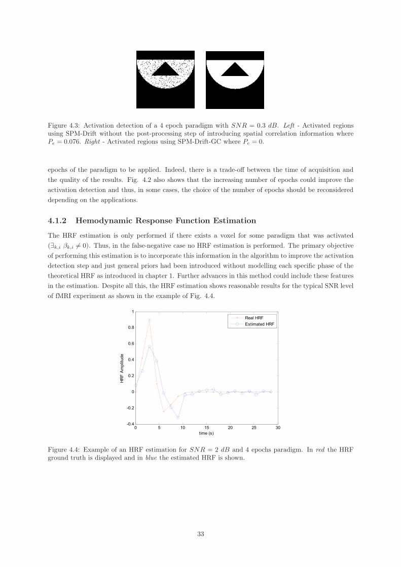
Figure 4.3: Activation detection of a 4 epoch paradigm with SNR = 0.3 dB. Left - Activated regionsusing SPM-Drift without the post-processing step of introducing spatial correlation information wherePe = 0.076. Right - Activated regions using SPM-Drift-GC where Pe = 0.

epochs of the paradigm to be applied. Indeed, there is a trade-off between the time of acquisition andthe quality of the results. Fig. 4.2 also shows that the increasing number of epochs could improve theactivation detection and thus, in some cases, the choice of the number of epochs should be reconsidereddepending on the applications.

4.1.2 Hemodynamic Response Function Estimation

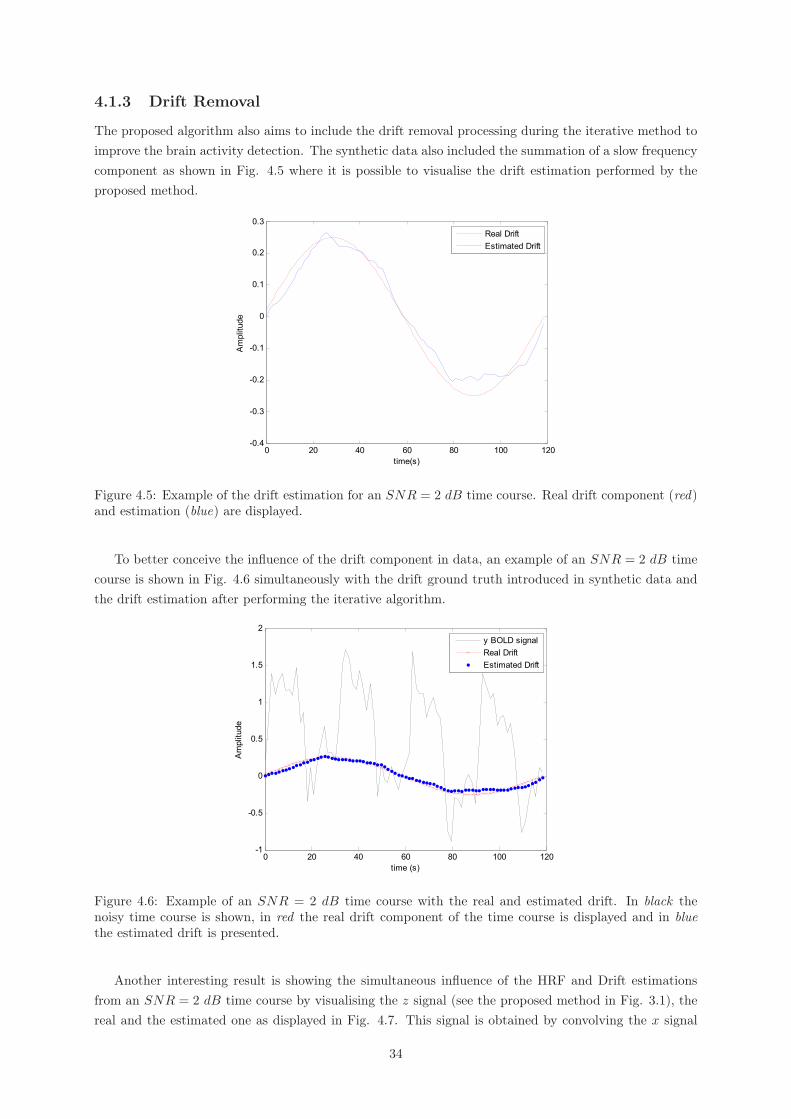
The HRF estimation is only performed if there exists a voxel for some paradigm that was activated(∃k,i βk,i �= 0). Thus, in the false-negative case no HRF estimation is performed. The primary objectiveof performing this estimation is to incorporate this information in the algorithm to improve the activationdetection step and just general priors had been introduced without modelling each specific phase of thetheoretical HRF as introduced in chapter 1. Further advances in this method could include these featuresin the estimation. Despite all this, the HRF estimation shows reasonable results for the typical SNR levelof fMRI experiment as shown in the example of Fig. 4.4.

0 5 10 15 20 25 30-0.4

-0.2

0

0.2

0.4

0.6

0.8

1

time (s)

HR

F A

mpl

itude

Real HRFEstimated HRF

Figure 4.4: Example of an HRF estimation for SNR = 2 dB and 4 epochs paradigm. In red the HRFground truth is displayed and in blue the estimated HRF is shown.

33

4.1.3 Drift Removal

The proposed algorithm also aims to include the drift removal processing during the iterative method toimprove the brain activity detection. The synthetic data also included the summation of a slow frequencycomponent as shown in Fig. 4.5 where it is possible to visualise the drift estimation performed by theproposed method.

0 20 40 60 80 100 120-0.4

-0.3

-0.2

-0.1

0

0.1

0.2

0.3

time(s)

Am

plitu

deReal DriftEstimated Drift

Figure 4.5: Example of the drift estimation for an SNR = 2 dB time course. Real drift component (red)and estimation (blue) are displayed.

To better conceive the influence of the drift component in data, an example of an SNR = 2 dB timecourse is shown in Fig. 4.6 simultaneously with the drift ground truth introduced in synthetic data andthe drift estimation after performing the iterative algorithm.

0 20 40 60 80 100 120-1

-0.5

0

0.5

1

1.5

2

time (s)

Am

plitu

de

y BOLD signalReal DriftEstimated Drift

Figure 4.6: Example of an SNR = 2 dB time course with the real and estimated drift. In black thenoisy time course is shown, in red the real drift component of the time course is displayed and in bluethe estimated drift is presented.

Another interesting result is showing the simultaneous influence of the HRF and Drift estimationsfrom an SNR = 2 dB time course by visualising the z signal (see the proposed method in Fig. 3.1), thereal and the estimated one as displayed in Fig. 4.7. This signal is obtained by convolving the x signal

34

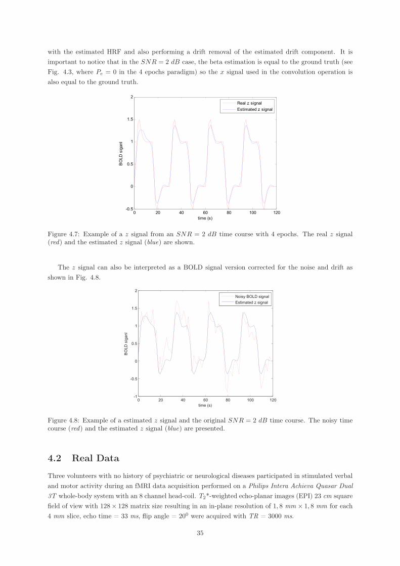
with the estimated HRF and also performing a drift removal of the estimated drift component. It isimportant to notice that in the SNR = 2 dB case, the beta estimation is equal to the ground truth (seeFig. 4.3, where Pe = 0 in the 4 epochs paradigm) so the x signal used in the convolution operation isalso equal to the ground truth.

0 20 40 60 80 100 120-0.5

0

0.5

1

1.5

2

time (s)

BO

LD s

igan

l

Real z signalEstimated z signal

Figure 4.7: Example of a z signal from an SNR = 2 dB time course with 4 epochs. The real z signal(red) and the estimated z signal (blue) are shown.

The z signal can also be interpreted as a BOLD signal version corrected for the noise and drift asshown in Fig. 4.8.

0 20 40 60 80 100 120-1

-0.5

0

0.5

1

1.5

2

time (s)

BO

LD

sig

anl

Noisy BOLD signal

Estimated z signal

Figure 4.8: Example of a estimated z signal and the original SNR = 2 dB time course. The noisy timecourse (red) and the estimated z signal (blue) are presented.

4.2 Real Data

Three volunteers with no history of psychiatric or neurological diseases participated in stimulated verbaland motor activity during an fMRI data acquisition performed on a Philips Intera Achieva Quasar Dual3T whole-body system with an 8 channel head-coil. T2*-weighted echo-planar images (EPI) 23 cm squarefield of view with 128× 128 matrix size resulting in an in-plane resolution of 1, 8 mm × 1, 8 mm for each4 mm slice, echo time = 33 ms, flip angle = 200 were acquired with TR = 3000 ms.

35

The paradigms were all structured on the same block-design, with 20 samples per epoch (10 samplesof stimulus followed by 10 samples of baseline, summing up to 60 s time per epoch) in a total of 4 epochs.Table 4.1 presents the paradigms applied to the subject.

Table 4.1: Description of the paradigms applied to the subjects

Right Foot Stimulus Moving right foot toesBaseline Complete rest with closed eyes

Tongue Stimulus Moving the tongue side to sideBaseline Stop the tongue movement

Verb generation Stimulus Seeing nouns and thinking about the related verbsBaseline Seeing the "####" string

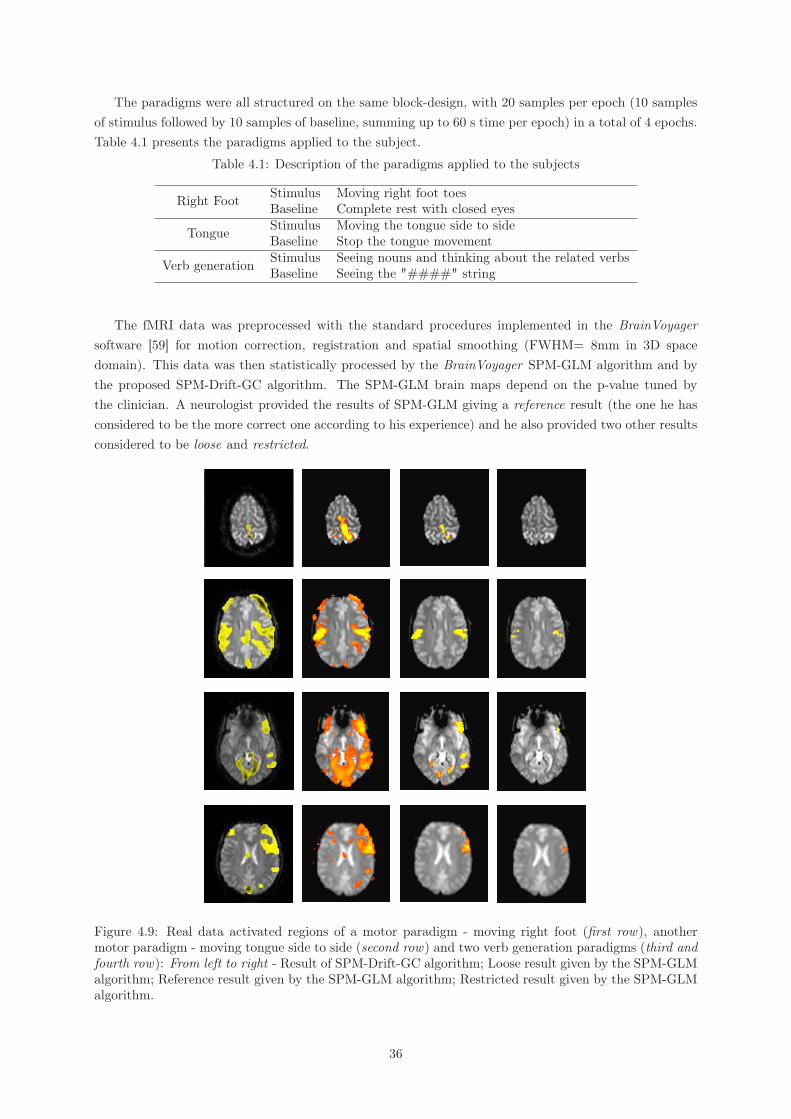
The fMRI data was preprocessed with the standard procedures implemented in the BrainVoyagersoftware [59] for motion correction, registration and spatial smoothing (FWHM= 8mm in 3D spacedomain). This data was then statistically processed by the BrainVoyager SPM-GLM algorithm and bythe proposed SPM-Drift-GC algorithm. The SPM-GLM brain maps depend on the p-value tuned bythe clinician. A neurologist provided the results of SPM-GLM giving a reference result (the one he hasconsidered to be the more correct one according to his experience) and he also provided two other resultsconsidered to be loose and restricted.

� � � �

� � � �

� � � �

� �

Figure 4.9: Real data activated regions of a motor paradigm - moving right foot (first row), anothermotor paradigm - moving tongue side to side (second row) and two verb generation paradigms (third andfourth row): From left to right - Result of SPM-Drift-GC algorithm; Loose result given by the SPM-GLMalgorithm; Reference result given by the SPM-GLM algorithm; Restricted result given by the SPM-GLMalgorithm.

36

The activated regions of SPM-Drift-CG algorithm are coded with color intensity gradient, inverselyproportional to the energy function of one of the equivalent equations ((3.26), (3.27) or (3.28)). Thisapplied colormap gives an important perception of the confidence of these results since the low intensityregions correspond to a higher value of the energy function (see equations (3.26), (3.27) or (3.28)) thatis being minimized.

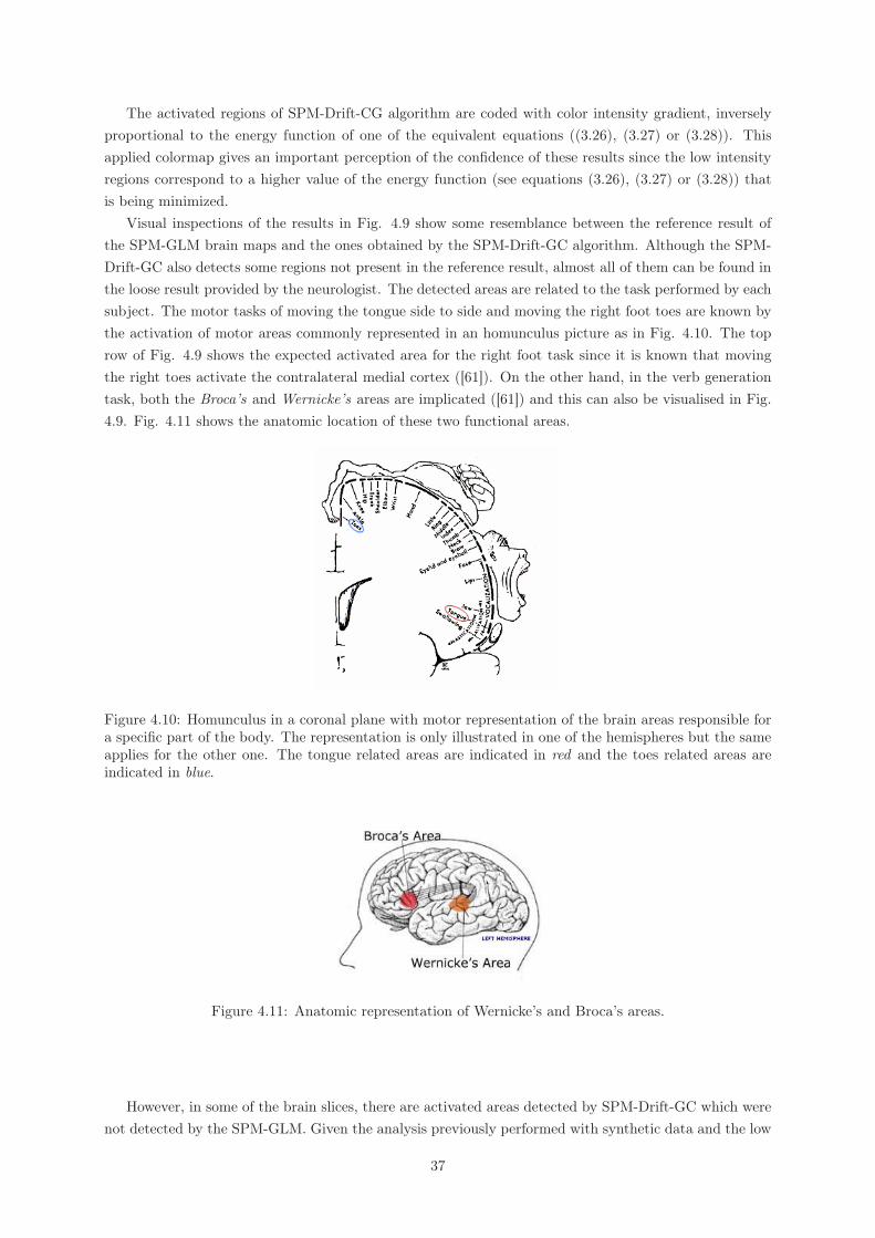
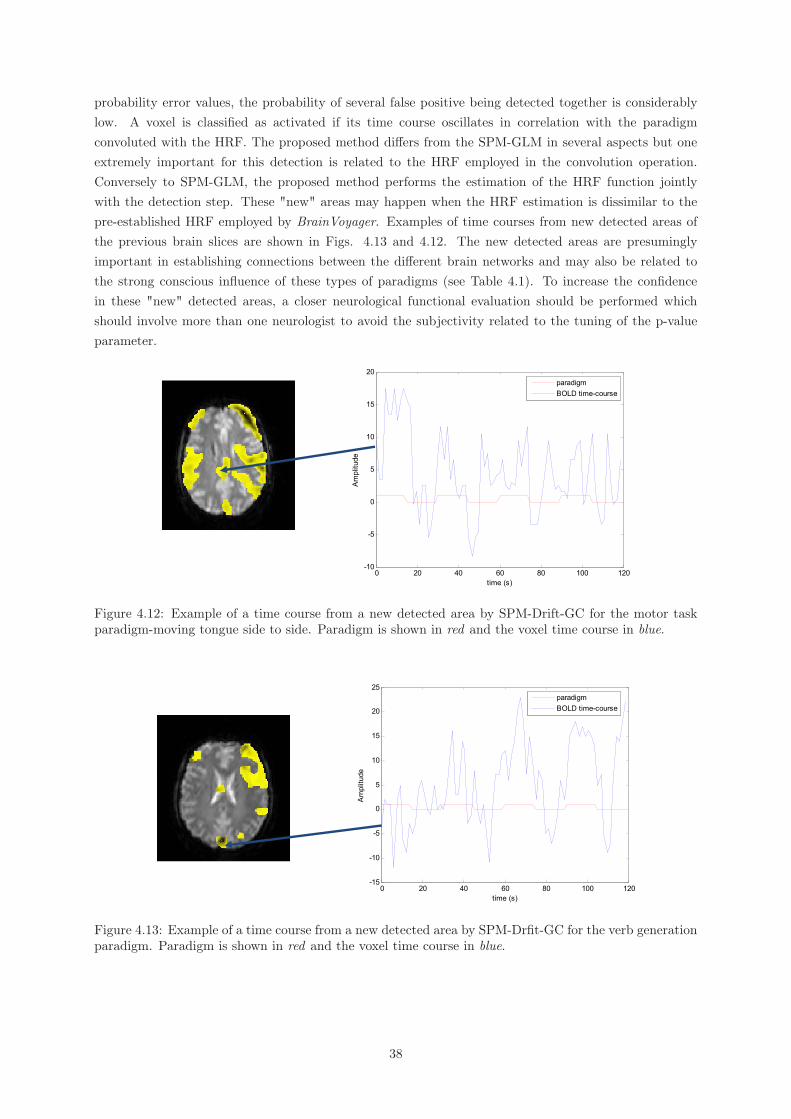
Visual inspections of the results in Fig. 4.9 show some resemblance between the reference result ofthe SPM-GLM brain maps and the ones obtained by the SPM-Drift-GC algorithm. Although the SPM-Drift-GC also detects some regions not present in the reference result, almost all of them can be found inthe loose result provided by the neurologist. The detected areas are related to the task performed by eachsubject. The motor tasks of moving the tongue side to side and moving the right foot toes are known bythe activation of motor areas commonly represented in an homunculus picture as in Fig. 4.10. The toprow of Fig. 4.9 shows the expected activated area for the right foot task since it is known that movingthe right toes activate the contralateral medial cortex ([61]). On the other hand, in the verb generationtask, both the Broca’s and Wernicke’s areas are implicated ([61]) and this can also be visualised in Fig.4.9. Fig. 4.11 shows the anatomic location of these two functional areas.

Figure 4.10: Homunculus in a coronal plane with motor representation of the brain areas responsible fora specific part of the body. The representation is only illustrated in one of the hemispheres but the sameapplies for the other one. The tongue related areas are indicated in red and the toes related areas areindicated in blue.

Figure 4.11: Anatomic representation of Wernicke’s and Broca’s areas.

However, in some of the brain slices, there are activated areas detected by SPM-Drift-GC which werenot detected by the SPM-GLM. Given the analysis previously performed with synthetic data and the low

37

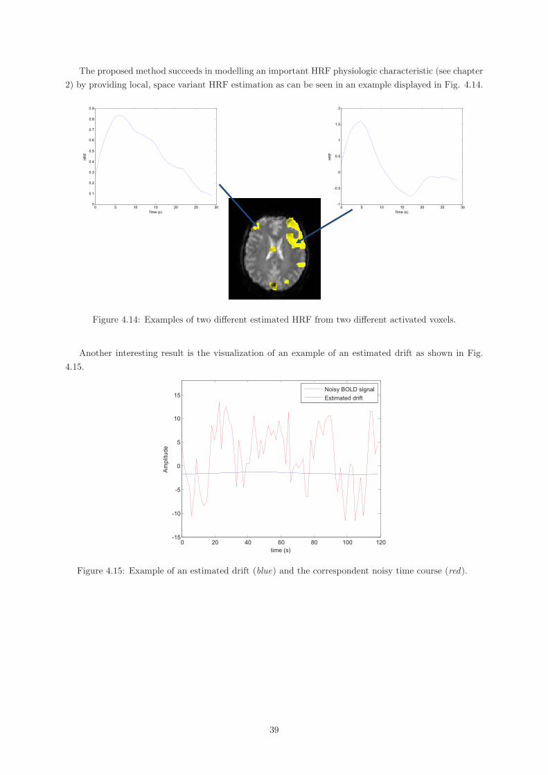
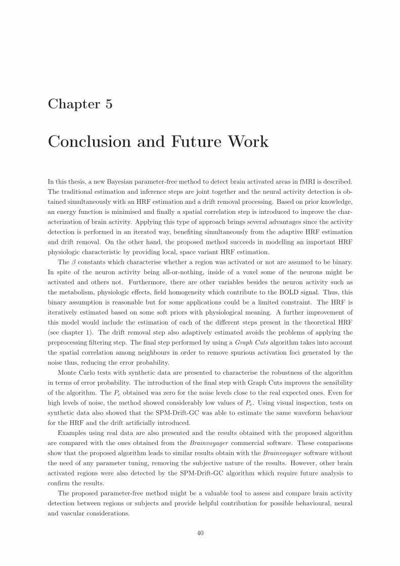
probability error values, the probability of several false positive being detected together is considerablylow. A voxel is classified as activated if its time course oscillates in correlation with the paradigmconvoluted with the HRF. The proposed method differs from the SPM-GLM in several aspects but oneextremely important for this detection is related to the HRF employed in the convolution operation.Conversely to SPM-GLM, the proposed method performs the estimation of the HRF function jointlywith the detection step. These "new" areas may happen when the HRF estimation is dissimilar to thepre-established HRF employed by BrainVoyager. Examples of time courses from new detected areas ofthe previous brain slices are shown in Figs. 4.13 and 4.12. The new detected areas are presuminglyimportant in establishing connections between the different brain networks and may also be related tothe strong conscious influence of these types of paradigms (see Table 4.1). To increase the confidencein these "new" detected areas, a closer neurological functional evaluation should be performed whichshould involve more than one neurologist to avoid the subjectivity related to the tuning of the p-valueparameter.

0 20 40 60 80 100 120-10

-5

0

5

10

15

20

time (s)

Am

plitu

de

paradigmBOLD time-course

Figure 4.12: Example of a time course from a new detected area by SPM-Drift-GC for the motor taskparadigm-moving tongue side to side. Paradigm is shown in red and the voxel time course in blue.

�

�

�

�

�

�

� 0 20 40 60 80 100 120-15

-10

-5

0

5

10

15

20

25

time (s)

Am

plitu

de

paradigmBOLD time-course

Figure 4.13: Example of a time course from a new detected area by SPM-Drfit-GC for the verb generationparadigm. Paradigm is shown in red and the voxel time course in blue.

38

The proposed method succeeds in modelling an important HRF physiologic characteristic (see chapter2) by providing local, space variant HRF estimation as can be seen in an example displayed in Fig. 4.14.

0 5 10 15 20 25 30-1

-0.5

0

0.5

1

1.5

2

Time (s)

HR

F

0 5 10 15 20 25 300

0.1

0.2

0.3

0.4

0.5

0.6

0.7

0.8

0.9

Time (s)

HR

F

�

�

�

�

�

�

�

�

�

Figure 4.14: Examples of two different estimated HRF from two different activated voxels.

Another interesting result is the visualization of an example of an estimated drift as shown in Fig.4.15.

0 20 40 60 80 100 120-15

-10

-5

0

5

10

15

time (s)

Am

plit

ude

Noisy BOLD signal

Estimated drift

Figure 4.15: Example of an estimated drift (blue) and the correspondent noisy time course (red).

39

Chapter 5

Conclusion and Future Work

In this thesis, a new Bayesian parameter-free method to detect brain activated areas in fMRI is described.The traditional estimation and inference steps are joint together and the neural activity detection is ob-tained simultaneously with an HRF estimation and a drift removal processing. Based on prior knowledge,an energy function is minimised and finally a spatial correlation step is introduced to improve the char-acterization of brain activity. Applying this type of approach brings several advantages since the activitydetection is performed in an iterated way, benefiting simultaneously from the adaptive HRF estimationand drift removal. On the other hand, the proposed method succeeds in modelling an important HRFphysiologic characteristic by providing local, space variant HRF estimation.

The β constants which characterise whether a region was activated or not are assumed to be binary.In spite of the neuron activity being all-or-nothing, inside of a voxel some of the neurons might beactivated and others not. Furthermore, there are other variables besides the neuron activity such asthe metabolism, physiologic effects, field homogeneity which contribute to the BOLD signal. Thus, thisbinary assumption is reasonable but for some applications could be a limited constraint. The HRF isiteratively estimated based on some soft priors with physiological meaning. A further improvement ofthis model would include the estimation of each of the different steps present in the theoretical HRF(see chapter 1). The drift removal step also adaptively estimated avoids the problems of applying thepreprocessing filtering step. The final step performed by using a Graph Cuts algorithm takes into accountthe spatial correlation among neighbours in order to remove spurious activation foci generated by thenoise thus, reducing the error probability.

Monte Carlo tests with synthetic data are presented to characterise the robustness of the algorithmin terms of error probability. The introduction of the final step with Graph Cuts improves the sensibilityof the algorithm. The Pe obtained was zero for the noise levels close to the real expected ones. Even forhigh levels of noise, the method showed considerably low values of Pe. Using visual inspection, tests onsynthetic data also showed that the SPM-Drift-GC was able to estimate the same waveform behaviourfor the HRF and the drift artificially introduced.

Examples using real data are also presented and the results obtained with the proposed algorithmare compared with the ones obtained from the Brainvoyager commercial software. These comparisonsshow that the proposed algorithm leads to similar results obtain with the Brainvoyager software withoutthe need of any parameter tuning, removing the subjective nature of the results. However, other brainactivated regions were also detected by the SPM-Drift-GC algorithm which require future analysis toconfirm the results.

The proposed parameter-free method might be a valuable tool to assess and compare brain activitydetection between regions or subjects and provide helpful contribution for possible behavioural, neuraland vascular considerations.

40

Bibliography

[1] J. L. Prince and J. M. Links, Medical Imaging - Signals and Systems. Pearson Prentice HallBioengineering, 2006.

[2] R. S. Menon, S. Ogawa, X. Hu, J. P. Strupp, P. Anderson, and K. Uurbil, “BOLD Based FunctionalMRI at 4 Tesla Includes a Capillary Bed Contribution: Echo-Planar Imaging Correlates with Pre-vious Optical Imaging Using Intrinsic Signals,” Magnetic Resonance in Medicine, vol. 33, no. 3, pp.453–459, Nov 1995.

[3] J. Frahm, K.-D. Merboldt, W. Hänicke, A. Kleinschmidt, and H. Boecker, “Brain or vein - oxygena-tion or flow? On signal physiology in functional MRI of human brain activation,” NMR in Medicine,vol. 7, no. 1-2, pp. 45–53, 1994.

[4] A. L. Baert, M. Knauth, and M. Sartor, Clinical Functional MRI, C. Stippich, Ed. Springer-Verlag,2007.

[5] P. Jezzard, P. M. Matthews, and S. M. Smith, Functional magnetic resonance imaging: An intro-duction to methods. Oxford Medical Publications, 2006.

[6] “Functional MRI research center, columbia university.” [Online]. Available: http://www.fmri.org/

[7] P. Bandettini, E. Wong, R. Hinks, R. Tikofsky, and J. Hyde, “Time course EPI of human brainfunction during task activation,” Magnetic Resonance in Medicine, vol. 25, no. 2, pp. 390–397, 1992.

[8] K. K. Kwong, J. W. Belliveau, D. A. Chesler, I. E. Goldberg, R. M. Weisskoff, B. P. Poncelet,D. N. Kennedy, B. E. Hoppel, M. S. Cohen, and R. Turner, “Dynamic magnetic resonance imagingof human brain activity during primary sensory stimulation,” Proc. Natl. Acad. Sci. USA, vol. 89,no. 12, pp. 5675–5679, 1992.

[9] S. Ogawa, D. W. Tank, R. Menon, J. M. Ellermann, S. G. Kim, H. Merkle, and K. Ugurbil, “Intrinsicsignal changes accompanying sensory stimulation: Functional brain mapping using MRI,” Proc. Natl.Acad. Sci. USA, vol. 89, no. 13, pp. 5951–5955, Jul 1992.

[10] K. J. Friston, P. Jezzard, and R. Turner, “Analysis of functional MRI time-series,” Human BrainMapping, vol. 1, no. 2, pp. 153–171, Oct 2004.

[11] D. M. Afonso, J. Sanches, and M. H. Lauterbach, “Neural physiological modeling towards a hemo-dynamic response function for fMRI,” Conf Proc IEEE Eng Med Biol Soc, vol. 1, pp. 1615–1618,2007.

[12] S. Ogawa, T. M. Lee, A. R. Kay, and D. W. Tank, “Brain magnetic resonance imaging with contrastdependent on blood oxygenation,” Proc Natl Acad Sci U S A, vol. 87, no. 24, pp. 9868–9872, Dec1990.

41

[13] S. Ogawa, R. S. Menon, D. W. Tank, S. G. Kim, H. Merkle, J. M. Ellermann, and K. Ugurbil, “Func-tional brain mapping by blood oxygenation level-dependent contrast magnetic resonance imaging. acomparison of signal characteristics with a biophysical model,” Biophysical Journal, vol. 64, no. 3,pp. 803–812, Mar 1993.

[14] N. K. Logothetis, “The Underpinnings of the BOLD Functional Magnetic Resonance Imaging Signal,”The Journal of Neuroscience, vol. 23, no. 10, pp. 3963–3971, May 2003.

[15] N. K. Logothetis, J. Pauls, M. Augath, T. Trinath, and A. Oeltermann, “Investigation of the Basisof the fMRI signal,” Nature, vol. 412, 2001.

[16] N. K. Logothetis, “The neural basis of the blood-oxygen-level-dependent functional magnetic reso-nance imaging signal,” Philos Trans R Soc Lond B Biol Sci., vol. 357, no. 1424, pp. 1003–1037, Aug2002.

[17] N. K. Logothetis and B. A. Wandell, “Interpreting the BOLD signal,” Annual Review of Physiology,vol. 66, 2004.

[18] J. Gati, R. S. Menon, K. Ugurbil, and B. K. Rutt, “Experimental determination of the BOLD fieldstrength dependence in vessels and tissue,” Magnetic Resonance in Medicine, vol. 38, no. 2, pp.296–302, Aug 1997.

[19] K. Thulborn, “Clinical rationale for very high field (3.0 Tesla) functional MR imaging,” TopicsMagnetic Resonance, vol. 10, no. 1, pp. 37–50, Feb 1999.

[20] K. R. Thulborn, “Clinical functional Magnetic Resonance Imaging,” in Current Protocols in MagneticResonance Imaging, 2006.

[21] C. Triantafyllou, R. Hoge, G. Krueger, C. Wiggins, A. Potthast, G. Wiggins, and L. Wald, “Com-parison of physiological noise at 1.5T, 3T and 7T and optimization of fMRI acquisition parameters,”NeuroImage, vol. 26, no. 1, pp. 243–250, May 2005.

[22] J. Coelho, J. Sanches, and M. H. Lauterbach, “fMRI Binary Detection of Brain Activated Regionswith Graph-Cuts,” Conf Proc IEEE Eng Med Biol Soc, vol. 1, pp. 4411–4414, 2008.

[23] J. Coelho, J. Sanches, and M. Lauterbach, “Brain activity detection with Graph Cuts,” Out 2008.

[24] K. M. Petersson, T. Nichols, J.-B. Poline, and A. Holmes, “Statistical limitations in functionalneuroimaging I. Non-inferential methods and statistical models,” The Royal Society, vol. 354, 1999.

[25] K. Friston, C. Frith, P. Liddle, and R. Frackowiak, “Comparing functional (PET) images: Theassessment of significant change,” Journal of Cerebral Blood Flow and Metabolism, vol. 11, pp. 690–699, 1991.

[26] K. Friston, J. Ashburner, S. Kiebel, T. Nichols, and W. Penny, Eds., Statistical Parametric Mapping:The Analysis of Functional Brain Images. Academic Press, 2007.

[27] K. J. Friston, W. Penny, C. Phillips, S. Kiebel, G. Hinton, and J. Ashburner, “Classical and Bayesianinference in neuroimaging: Theory,” NeuroImage, vol. 16, pp. 465–483, 2002.

[28] K. Friston, “Analyzing brain images: Principles and overview,” Human Brain Function, pp. 25–41,1997.

42

[29] P. L. Purdon and R. M. Weisskoff, “Effect of temporal autocorrelation due to physiological noise andstimulus paradigm on voxel-level false-positive rates in fMRI,” Human Brain Mapping, vol. 6, pp.239–249, 1998.

[30] K. Friston, “Models of brain function in neuroimaging,” in Annu. Rev. Psychol.

[31] A. Gelman, J. B. Carlin, H. S. Stern, and D. B. Rubin, Bayesian Data Analysis, Second Edition.Chapman & Hall/CRC, July 2003.

[32] K. M. Hanson, “Introduction to Bayesian image analysis,” Medical imaging VII: image processing(ed. M. H. Loew), Proc. SPIE, vol. 1898, no. 8, pp. 716–731, 1993.

[33] C. R. Vogel, Computational methods for inverse problems, ser. Frontiers in applied mathematics,2002.

[34] G. E. Box and G. C. Tiao, Bayesian Inference in Statistical Analysis (Wiley Classics Library).Wiley-Interscience, April 1992.

[35] G. Marrelec, H. Benali, P. Ciuciu, M. Pélégrini-Issac, and J.-B. Poline, “Robust Bayesian estima-tion of the hemodynamic response function in event-related BOLD fMRI using basic physiologicalinformation,” Human Brain Mapping, vol. 19, pp. 1–17, 2003.

[36] D. M. Afonso, J. M. Sanches, and M. H. Lauterbach, “Robust brain activation detection in functionalMRI,” IEEE International Conference on Image Processing, October.

[37] R. Cotterill, Ed., Biophysics: An Introduction. Wiley, 2002.

[38] S. D. Forman, J. D. Cohen, M. Fitzgerald, W. F. Eddy, M. A. Mintun, and D. C. Noll, “Improvedassessment of significant activation in functional magnetic resonance imaging (fMRI): Use of a cluster-size threshold,” Magnetic Resonance in Medicine, vol. 33, pp. 636–647, 1995.

[39] N. A. Lazar, W. F. Eddy, C. R. Genovese, and J. Welling, “Statistical issues in (fMRI) for brainimaging,” International Statistical Review, vol. 69, no. 1, 2007.

[40] X. Descombes, F. Kruggel, and D. Y. V. Cramon, “Spatio-temporal fMRI analysis using markov ran-dom fields,” IEEE Transactions on Biomedical Engineering, vol. 17, no. 6, pp. 1028–1039, December1998.

[41] S. Kirkpatrick, C. D. Gelatt, and M. P. Vecchi, “Optimization by simulated annealing,” Science, vol.220, pp. 671–680, 1983.

[42] K. Katanoda, Y. Matsuda, and M. Sugishita, “A spatio-temporal regression model for the analysisof functional MRI data,” NeuroImage, vol. 17, pp. 1415–1428, 2002.

[43] H. Luo and S. Puthusserypady, “Analysis of fMRI data with drift: Modified general linear model andbayesian estimator,” IEEE Transactions on Biomedical Engineering, vol. 55, no. 5, pp. 1504–1511,May 2008.

[44] A. M. Smith, B. K. Lewis, U. E. Ruttimann, F. Q. Ye, T. M. Sinnwell, Y. Yang, J. H. Duyn, andJ. A. Frank, “Investigation of low frequency drift in fMRI signal,” NeuroImage, vol. 9, no. 5, pp.526–533, 1999.

[45] J. Brosch, T. Talavage, J. Ulmer, and J. Nyenhuis, “Simulation of human respiration in fMRI with amechanical model,” IEEE Transactions on Biomedical Engineering, vol. 49, no. 7, pp. 700–707, July2002.

43

[46] ——, “Deconvolution of event-related fMRI responses in fast-rate experimental designs: Trackingamplitude variations,” Journal Cognitive Neuroscience, vol. 12, no. 2, pp. 76–89, November 2000.

[47] C. Long, E. Brown, C. Triantafyllou, I. Aharon, L. Wald, and V. Solo, “Nonstationary noise estima-tion in functional MRI,” NeuroImage, vol. 28, no. 4, pp. 890–903, December 2005.

[48] R. Frackowiak, K. Friston, C. Frith, R. Dolan, C. Price, S. Zeki, J. Ashburner, and W. Penny, HumanBrain Function, 2nd ed. Academic Press, 2003.

[49] Y. Boykov, O. Veksler, and R. Zabih, “Fast approximate energy minimization via graph cuts,” IEEETrans. Pattern Anal. Mach. Intell., vol. 23, no. 11, pp. 1222–1239, 2001.

[50] A. M. Dale and R. L. Buckner, “Selective averaging of rapidly presented individual trials using fMRI,”Human Brain Mapping.

[51] R. L. Buckner, “Event-related fMRI and the hemodynamic response,” Human Brain Mapping, vol. 6,pp. 373–377, 1998.

[52] A. M. Wink and J. B. Roerdink, “Denoising functional MR images: a comparison of wavelet de-noising and Gaussian smoothing,” IEEE Trans Med Imaging, vol. 23, no. 3, pp. 374–387, Mar 2004,comparative Study.

[53] J. Sanches and J. S. Marques, “A map estimation algorithm using IIR recursive filters,” in Pro-ceedings International Workshop on Energy Minimization Methods in Computer Vision and PatternRecognition, 2003.

[54] T. K. Moon and W. C. Stirling, Mathematical methods and algorithms for signal processing, 2000.

[55] S. Geman and D. Geman, “Stochastic relaxation, gibbs distributions, and the bayesian restorationof images,” IEEE Trans. Pattern Analysis and Machine Intelligence, vol. 6, pp. 721–741, November1984.

[56] K. J. Friston, P. Fletcher, O. Josephs, A. Holmes, M. D. Rugg, and R. Turner, “Event-related fMRI:Characterizing differential responses,” NeuroImage, vol. 7, no. 1, pp. 30–40, January 1998.

[57] V. Kolmogorov and R. Zabih, “What energy functions can be minimized via graph cuts?” IEEETrans. Pattern Anal. Mach. Intell., vol. 26, no. 2, pp. 147–159, 2004.

[58] Y. Boykov, V. S. Lee, H. Rusinek, and R. Bansal, “Segmentation of dynamic N-D data sets viaGraph Cuts using Markov Models,” in Proceedings of Medical Image Computing and Computer-Assisted Intervention, 2001.

[59] “Brainvoyager software.” [Online]. Available: http://www.brainvoyager.com/

[60] G. H. Glover, “On signal to noise ratio tradeoffs in fMRI,” Apr 1999.

[61] R. S. Snell, Clinical Neuroanatomy, 6th ed.

44

Chapter 6

Appendices

6.1 EMBC2008 Published Paper

45

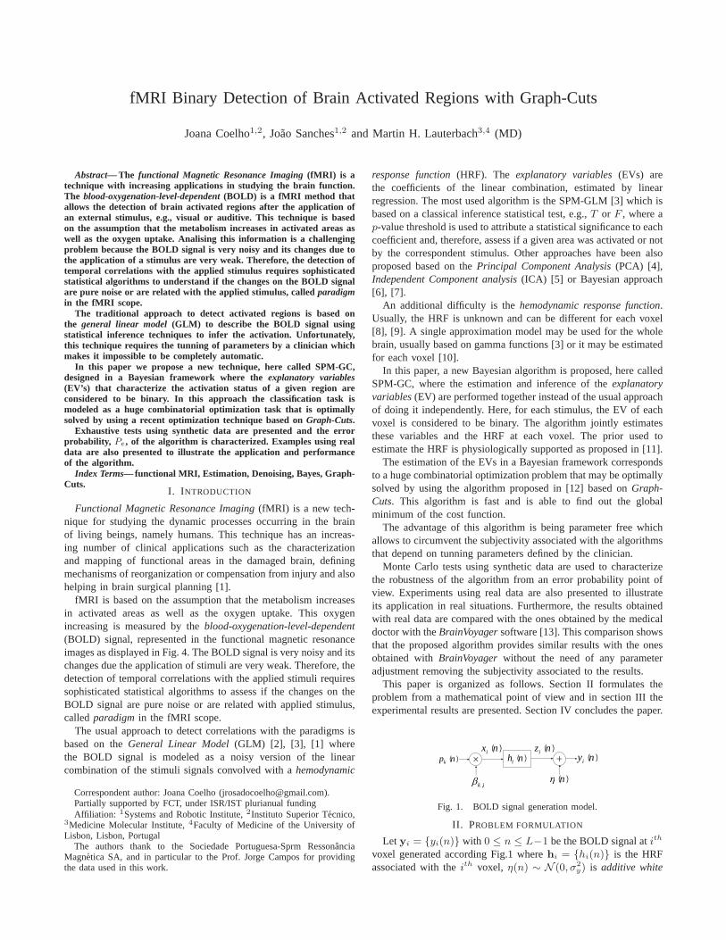
fMRI Binary Detection of Brain Activated Regions with Graph-Cuts

Joana Coelho1,2, Joao Sanches1,2 and Martin H. Lauterbach3,4 (MD)

Abstract— The functional Magnetic Resonance Imaging (fMRI) is atechnique with increasing applications in studying the brain function.The blood-oxygenation-level-dependent (BOLD) is a fMRI method thatallows the detection of brain activated regions after the application ofan external stimulus, e.g., visual or auditive. This technique is basedon the assumption that the metabolism increases in activated areas aswell as the oxygen uptake. Analising this information is a challengingproblem because the BOLD signal is very noisy and its changes due tothe application of a stimulus are very weak. Therefore, the detection oftemporal correlations with the applied stimulus requires sophisticatedstatistical algorithms to understand if the changes on the BOLD signalare pure noise or are related with the applied stimulus, called paradigmin the fMRI scope.

The traditional approach to detect activated regions is based onthe general linear model (GLM) to describe the BOLD signal usingstatistical inference techniques to infer the activation. Unfortunately,this technique requires the tunning of parameters by a clinician whichmakes it impossible to be completely automatic.

In this paper we propose a new technique, here called SPM-GC,designed in a Bayesian framework where the explanatory variables(EV’s) that characterize the activation status of a given region areconsidered to be binary. In this approach the classification task ismodeled as a huge combinatorial optimization task that is optimallysolved by using a recent optimization technique based on Graph-Cuts.

Exhaustive tests using synthetic data are presented and the errorprobability, Pe, of the algorithm is characterized. Examples using realdata are also presented to illustrate the application and performanceof the algorithm.

Index Terms— functional MRI, Estimation, Denoising, Bayes, Graph-Cuts.

I. INTRODUCTION

Functional Magnetic Resonance Imaging (fMRI) is a new tech-nique for studying the dynamic processes occurring in the brainof living beings, namely humans. This technique has an increas-ing number of clinical applications such as the characterizationand mapping of functional areas in the damaged brain, definingmechanisms of reorganization or compensation from injury and alsohelping in brain surgical planning [1].

fMRI is based on the assumption that the metabolism increasesin activated areas as well as the oxygen uptake. This oxygenincreasing is measured by the blood-oxygenation-level-dependent(BOLD) signal, represented in the functional magnetic resonanceimages as displayed in Fig. 4. The BOLD signal is very noisy and itschanges due the application of stimuli are very weak. Therefore, thedetection of temporal correlations with the applied stimuli requiressophisticated statistical algorithms to assess if the changes on theBOLD signal are pure noise or are related with applied stimulus,called paradigm in the fMRI scope.

The usual approach to detect correlations with the paradigms isbased on the General Linear Model (GLM) [2], [3], [1] wherethe BOLD signal is modeled as a noisy version of the linearcombination of the stimuli signals convolved with a hemodynamic

Correspondent author: Joana Coelho (jrosadocoelho@gmail.com).Partially supported by FCT, under ISR/IST plurianual fundingAffiliation: 1Systems and Robotic Institute, 2Instituto Superior Tecnico,

3Medicine Molecular Institute, 4Faculty of Medicine of the University ofLisbon, Lisbon, Portugal

The authors thank to the Sociedade Portuguesa-Sprm RessonanciaMagnetica SA, and in particular to the Prof. Jorge Campos for providingthe data used in this work.

response function (HRF). The explanatory variables (EVs) arethe coefficients of the linear combination, estimated by linearregression. The most used algorithm is the SPM-GLM [3] which isbased on a classical inference statistical test, e.g., T or F , where ap-value threshold is used to attribute a statistical significance to eachcoefficient and, therefore, assess if a given area was activated or notby the correspondent stimulus. Other approaches have been alsoproposed based on the Principal Component Analysis (PCA) [4],Independent Component analysis (ICA) [5] or Bayesian approach[6], [7].

An additional difficulty is the hemodynamic response function.Usually, the HRF is unknown and can be different for each voxel[8], [9]. A single approximation model may be used for the wholebrain, usually based on gamma functions [3] or it may be estimatedfor each voxel [10].

In this paper, a new Bayesian algorithm is proposed, here calledSPM-GC, where the estimation and inference of the explanatoryvariables (EV) are performed together instead of the usual approachof doing it independently. Here, for each stimulus, the EV of eachvoxel is considered to be binary. The algorithm jointly estimatesthese variables and the HRF at each voxel. The prior used toestimate the HRF is physiologically supported as proposed in [11].

The estimation of the EVs in a Bayesian framework correspondsto a huge combinatorial optimization problem that may be optimallysolved by using the algorithm proposed in [12] based on Graph-Cuts. This algorithm is fast and is able to find out the globalminimum of the cost function.

The advantage of this algorithm is being parameter free whichallows to circumvent the subjectivity associated with the algorithmsthat depend on tunning parameters defined by the clinician.

Monte Carlo tests using synthetic data are used to characterizethe robustness of the algorithm from an error probability point ofview. Experiments using real data are also presented to illustrateits application in real situations. Furthermore, the results obtainedwith real data are compared with the ones obtained by the medicaldoctor with the BrainVoyager software [13]. This comparison showsthat the proposed algorithm provides similar results with the onesobtained with BrainVoyager without the need of any parameteradjustment removing the subjectivity associated to the results.

This paper is organized as follows. Section II formulates theproblem from a mathematical point of view and in section III theexperimental results are presented. Section IV concludes the paper.

)(npk)(nhi

)(n

)(nyi

ik,

)(nxi )(nzi

Fig. 1. BOLD signal generation model.

II. PROBLEM FORMULATION

Let yi = {yi(n)} with 0 ≤ n ≤ L−1 be the BOLD signal at ith

voxel generated according Fig.1 where hi = {hi(n)} is the HRFassociated with the ith voxel, η(n) ∼ N (0, σ2

y) is additive white

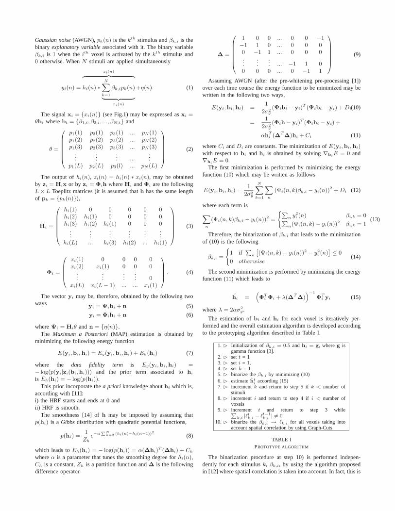
Gaussian noise (AWGN), pk(n) is the kth stimulus and βk,i is thebinary explanatory variable associated with it. The binary variableβk,i is 1 when the ith voxel is activated by the kth stimulus and0 otherwise. When N stimuli are applied simultaneously

yi(n) =

zi(n)︷ ︸︸ ︷hi(n) ∗

N∑k=1

βk,ipk(n)

︸ ︷︷ ︸xi(n)

+η(n). (1)

The signal xi = {xi(n)} (see Fig.1) may be expressed as xi =θbi where bi = {β1,i, β2,i, ..., βN,i} and

θ =

⎛⎜⎜⎜⎜⎜⎝

p1(1) p2(1) p3(1) ... pN (1)p1(2) p2(2) p3(2) ... pN (2)p1(3) p2(3) p3(3) ... pN (3)

......

... ......

p1(L) p2(L) p3(l) ... pN (L)

⎞⎟⎟⎟⎟⎟⎠

(2)

The output of hi(n), zi(n) = hi(n) ∗ xi(n), may be obtainedby zi = Hix or by zi = Φih where Hi and Φi are the followingL × L Toeplitz matrices (it is assumed that h has the same lengthof pk = {pk(n)}),

Hi =

⎛⎜⎜⎜⎜⎜⎝

hi(1) 0 0 0 0 0hi(2) hi(1) 0 0 0 0hi(3) hi(2) hi(1) 0 0 0

......

......

......

hi(L) ... hi(3) hi(2) ... hi(1)

⎞⎟⎟⎟⎟⎟⎠

(3)

Φi =

⎛⎜⎜⎜⎝

xi(1) 0 0 0 0xi(2) xi(1) 0 0 0

......

...... 0

xi(L) xi(L − 1) ... ... xi(1)

⎞⎟⎟⎟⎠ . (4)

The vector yi may be, therefore, obtained by the following twoways yi = Ψibi + n (5)

yi = Φihi + n (6)

where Ψi = Hiθ and n = {η(n)}.The Maximum a Posteriori (MAP) estimation is obtained by

minimizing the following energy function

E(yi,bi,hi) = Ey(yi,bi,hi) + Eh(hi) (7)

where the data fidelity term is Ey(yi,bi,hi) =− log(p(yi|zi(bi,hi))) and the prior term associated to hi

is Eh(hi) = − log(p(hi)).This prior incorporate the a priori knowledge about hi which is,

according with [11]:i) the HRF starts and ends at 0 andii) HRF is smooth.

The smoothness [14] of h may be imposed by assuming thatp(hi) is a Gibbs distribution with quadratic potential functions,

p(hi) =1

Zhe−α

∑Nn=2 (hi(n)−hi(n−1))2 (8)

which leads to Eh(hi) = − log(p(hi)) = α(∆hi)T (∆hi) + Ch

where α is a parameter that tunes the smoothing degree for hi(n),Ch is a constant, Zh is a partition function and ∆ is the followingdifference operator

∆ =

⎛⎜⎜⎜⎜⎜⎝

1 0 0 ... 0 0 −1−1 1 0 ... 0 0 00 −1 1 ... 0 0 0...

...... ... −1 1 0

0 0 0 ... 0 −1 1

⎞⎟⎟⎟⎟⎟⎠

(9)

Assuming AWGN (after the pre-whitening pre-processing [1])over each time course the energy function to be minimized may bewritten in the following two ways,

E(yi,bi,hi) =1

2σ2y

(Ψibi − yi)T (Ψibi − yi) + Di(10)

=1

2σ2y

(Φih − yi)T (Φihi − yi) +

αhTi (∆T ∆)hi + Ci (11)

where Ci and Di are constants. The minimization of E(yi,bi,hi)with respect to bi and hi is obtained by solving ∇biE = 0 and∇hiE = 0.

The first minimization is performed by minimizing the energyfunction (10) which may be written as folllows

E(yi,bi,hi) =1

2σ2y

N∑k=1

∑n

(Ψi(n, k)βk,i − yi(n))2 + Di (12)

where each term is

∑n

(Ψi(n, k)βk,i − yi(n))2 =

{∑n y2

i (n) βi,k = 0∑n(Ψi(n, k) − yi(n))2 βi,k = 1

(13)

Therefore, the binarization of βk,i that leads to the minimizationof (10) is the following

βk,i =

{1 if

∑n

[(Ψi(n, k) − yi(n))2 − y2

i (n)] ≤ 0

0 otherwise(14)

The second minimization is performed by minimizing the energyfunction (11) which leads to

hi =(ΦT

i Φi + λ(∆T ∆))−1

ΦTi yi (15)

where λ = 2ασ2y .

The estimation of bi and hi for each voxel is iteratively per-formed and the overall estimation algorithm is developed accordingto the prototyping algorithm described in Table I.

1. � Initialization of βk,i = 0.5 and hi = g, where g isgamma function [3].

2. � set t = 13. � set i = 1,4. � set k = 15. � binarize the βk,i by minimizing (10)6. � estimate ht

i according (15)7. � increment k and return to step 5 if k < number of

stimuli8. � increment i and return to step 4 if i < number of

voxels9. � increment t and return to step 3 while∑

k,i |�tk,i − �t−1

k,i | �= 010. � binarize the βk,i → �k,i for all voxels taking into

account spatial correlation by using Graph-Cuts

TABLE IPROTOTYPE ALGORITHM

The binarization procedure at step 10) is performed indepen-dently for each stimulus k, βk,i, by using the algorithm proposedin [12] where spatial correlation is taken into account. In fact, this is

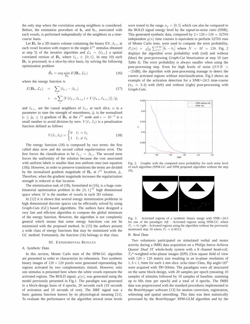
the only step where the correlation among neighbors is considered.Before, the estimation procedure of hi and bi, associated witheach voxels, is performed independently of the neighbors in a time-course basis.

Let Bk be a 3D matrix volume containing the binary EV, βk,i, ateach voxel location with respect to the single kth stimulus obtainedat step 5) of the iterative algorithm and Lk = {�k,i} a spatialcorrelated version of Bk where �k,i ∈ {0, 1}. In step 10) eachBk is processed, in a slice-by-slice basis, by solving the followingoptimization problem

Bk = arg minBk

E(Bk,Lk) (16)

where the energy function is

E(Bk,Lk) =∑

i

|�k,i − βk,i| (17)

+ α∑

i

[V (�k,i, �k,ih) + V (�k,i, �k,iv ))] /gi

and �k,iτ are the causal neighbors of �k,i at each slice, α is aparameter to tune the strength of smoothness, gi is the normalized(ε ≤ gk ≤ 1) gradient of Bk at the ith node and ε = 10−2 is asmall number to avoid division by zero. V (�1, �2) is a penalizationfunction defined as follows

V (�1, �2) =

{0 �1 = �2

1 �1 �= �2(18)

The energy function (18) is composed by two terms: the firstcalled data term and the second called regularization term. Thefirst forces the classification to be �k,i = βk,i. The second termforces the uniformity of the solution because the cost associatedwith uniform labels is smaller than non uniform ones (see equation(18)). However, in order to preserve transitions the terms are dividedby the normalized gradient magnitude of Bk at ith location, gi.Therefore, when the gradient magnitude increases the regularizationstrength is reduced at that location.

The minimization task of (18), formulated in (16), is a huge com-binatorial optimization problem in the {0, 1}M high dimensionalspace where M is the number of voxels in each 3D volume.

In [12] it is shown that several energy minimization problems inhigh dimensional discrete spaces can be efficiently solved by usingGraph-Cuts (GC) based algorithms. The authors have designed avery fast and efficient algorithm to compute the global minimumof the energy function. However, the algorithm is not completelygeneral which means that some energy functions can not beminimized with the proposed method. In [15] the authors presenta wide class of energy functions that may be minimized with theGC method. Fortunately, the function (16) belongs to that class.

III. EXPERIMENTAL RESULTS

A. Synthetic Data

In this section, Monte Carlo tests of the SPM-GC algorithmare presented in order to characterize its robustness. Two syntheticbinary images of 128× 128 pixels were generated representing theregions activated by two complementary stimuli. However, onlyone stimulus is presented here where the white voxels represent theactivated regions. The BOLD signal, y(n), was generated using themodel previously presented in Fig.1. The paradigm was generatedin a block-design basis of 4 epochs, 20 seconds each (10 secondsof activation and 10 seconds of rest). The HRF signal was abasic gamma function known by its physiological meaning [11].To evaluate the performance of the algorithm several noise levels

were tested in the range σy = [0; 5] which can also be compared tothe BOLD signal energy level by the signal-to-noise ratio (SNR).This generated synthetic data, composed by 2×128×128 = 32768independent y(n) time courses is equivalent to perform 32768 runsof Monte Carlo tests, were used to compute the error probability,Pe(σ) = 1

NM

∑NMi=1

∣∣∣bi − bi

∣∣∣ where N = M = 128. Fig. 2displays the algorithm error probability with (red) and without(blue) the post-processing Graph-Cut binarization at step 10 (seeTable I). The error probability is always smaller when using thepost-processing step. Even for high levels of noise (SNR >−25dB), the algorithm with post-processing manage to detect thecorrect activated regions without misclassification. Fig.3 shows anexample of the activation detection for a SNR=-24.5 time-course(σy = 3.4) with (left) and without (right) post-processing withGraph-Cuts.

−30 −25 −20 −15 −100

0.005

0.01

0.015

0.02

0.025

SNR

Pe

SPM without GCSPM−GC

Fig. 2. Graphic with the computed error probability for each noise levelof each algorithm (SPM-GC and SPM proposed algorithm without the step10).

Fig. 3. Activated regions of a synthetic binary image with SNR=-24.5for one of the paradigm: left - Activated regions using SPM-GC wherePe = 0; right - Activated regions using the algorithm without the previouslymentioned step 10 where Pe = 0.0012.

B. Real Data

Two volunteers participated on stimulated verbal and motoractivity during a fMRI data acquisition on a Philips Intera AchievaQuasar Dual 3T whole-body system with a 8 channel head-coil.T2*-weighted echo-planar images (EPI) 23cm square field of viewwith 128 × 128 matrix size resulting in an in-plane resolution of1, 8×1, 8mm for each 4 mm slice. echo time=33ms, flip angle=200

were acquired with TR=300ms. The paradigms were all structuredon the same block-design, with 20 samples per epoch (meaning 10samples of stimulus followed by 10 samples of baseline, summingup to 60s time per epoch) and a total of 4 epochs. The fMRIdata was preprocessed with the standard procedures implemented inthe BrainVoyager software [13] for motion correction, registration,whitening and spatial smoothing. This data was then statisticallyprocessed by the BrainVoyager SPM-GLM algorithm and by the

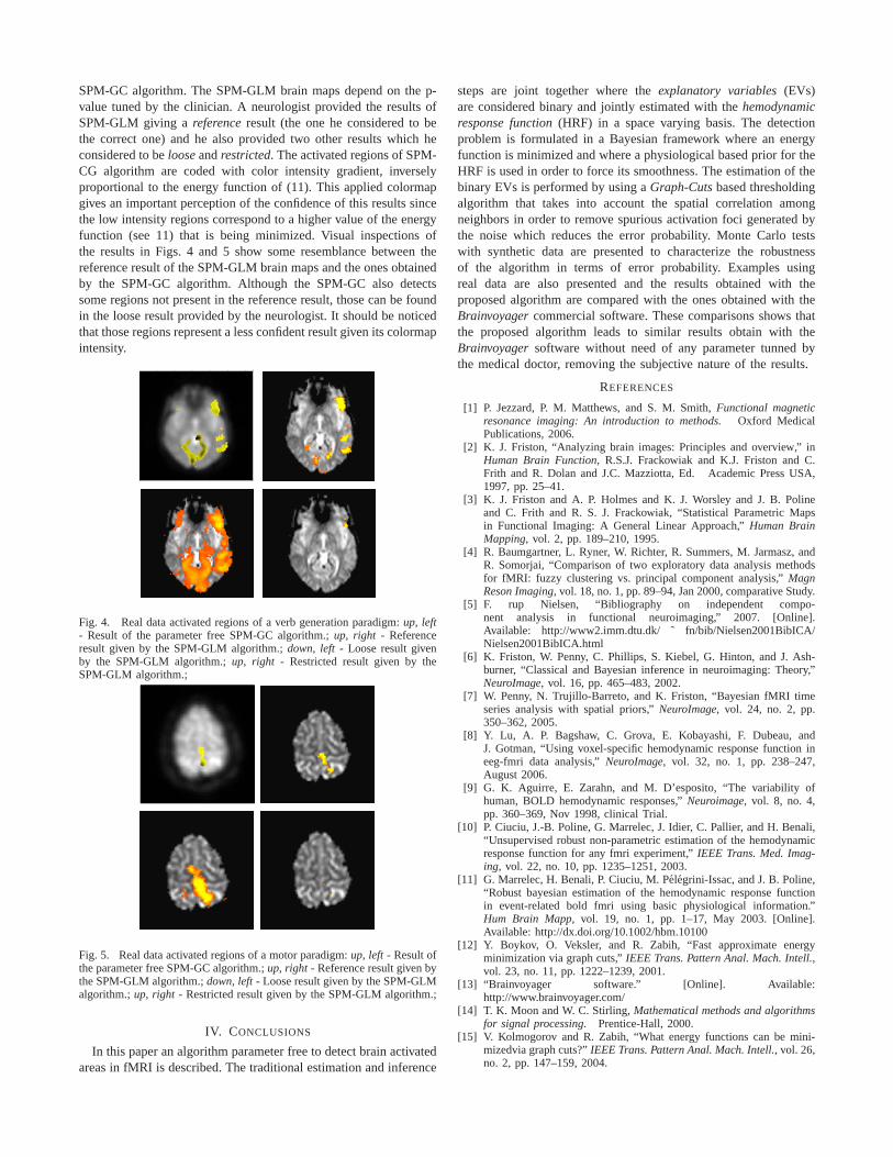
SPM-GC algorithm. The SPM-GLM brain maps depend on the p-value tuned by the clinician. A neurologist provided the results ofSPM-GLM giving a reference result (the one he considered to bethe correct one) and he also provided two other results which heconsidered to be loose and restricted. The activated regions of SPM-CG algorithm are coded with color intensity gradient, inverselyproportional to the energy function of (11). This applied colormapgives an important perception of the confidence of this results sincethe low intensity regions correspond to a higher value of the energyfunction (see 11) that is being minimized. Visual inspections ofthe results in Figs. 4 and 5 show some resemblance between thereference result of the SPM-GLM brain maps and the ones obtainedby the SPM-GC algorithm. Although the SPM-GC also detectssome regions not present in the reference result, those can be foundin the loose result provided by the neurologist. It should be noticedthat those regions represent a less confident result given its colormapintensity.

Fig. 4. Real data activated regions of a verb generation paradigm: up, left- Result of the parameter free SPM-GC algorithm.; up, right - Referenceresult given by the SPM-GLM algorithm.; down, left - Loose result givenby the SPM-GLM algorithm.; up, right - Restricted result given by theSPM-GLM algorithm.;

Fig. 5. Real data activated regions of a motor paradigm: up, left - Result ofthe parameter free SPM-GC algorithm.; up, right - Reference result given bythe SPM-GLM algorithm.; down, left - Loose result given by the SPM-GLMalgorithm.; up, right - Restricted result given by the SPM-GLM algorithm.;

IV. CONCLUSIONS

In this paper an algorithm parameter free to detect brain activatedareas in fMRI is described. The traditional estimation and inference

steps are joint together where the explanatory variables (EVs)are considered binary and jointly estimated with the hemodynamicresponse function (HRF) in a space varying basis. The detectionproblem is formulated in a Bayesian framework where an energyfunction is minimized and where a physiological based prior for theHRF is used in order to force its smoothness. The estimation of thebinary EVs is performed by using a Graph-Cuts based thresholdingalgorithm that takes into account the spatial correlation amongneighbors in order to remove spurious activation foci generated bythe noise which reduces the error probability. Monte Carlo testswith synthetic data are presented to characterize the robustnessof the algorithm in terms of error probability. Examples usingreal data are also presented and the results obtained with theproposed algorithm are compared with the ones obtained with theBrainvoyager commercial software. These comparisons shows thatthe proposed algorithm leads to similar results obtain with theBrainvoyager software without need of any parameter tunned bythe medical doctor, removing the subjective nature of the results.

REFERENCES

[1] P. Jezzard, P. M. Matthews, and S. M. Smith, Functional magneticresonance imaging: An introduction to methods. Oxford MedicalPublications, 2006.

[2] K. J. Friston, “Analyzing brain images: Principles and overview,” inHuman Brain Function, R.S.J. Frackowiak and K.J. Friston and C.Frith and R. Dolan and J.C. Mazziotta, Ed. Academic Press USA,1997, pp. 25–41.

[3] K. J. Friston and A. P. Holmes and K. J. Worsley and J. B. Polineand C. Frith and R. S. J. Frackowiak, “Statistical Parametric Mapsin Functional Imaging: A General Linear Approach,” Human BrainMapping, vol. 2, pp. 189–210, 1995.

[4] R. Baumgartner, L. Ryner, W. Richter, R. Summers, M. Jarmasz, andR. Somorjai, “Comparison of two exploratory data analysis methodsfor fMRI: fuzzy clustering vs. principal component analysis,” MagnReson Imaging, vol. 18, no. 1, pp. 89–94, Jan 2000, comparative Study.

[5] F. rup Nielsen, “Bibliography on independent compo-nent analysis in functional neuroimaging,” 2007. [Online].Available: http://www2.imm.dtu.dk/ ˜ fn/bib/Nielsen2001BibICA/Nielsen2001BibICA.html

[6] K. Friston, W. Penny, C. Phillips, S. Kiebel, G. Hinton, and J. Ash-burner, “Classical and Bayesian inference in neuroimaging: Theory,”NeuroImage, vol. 16, pp. 465–483, 2002.

[7] W. Penny, N. Trujillo-Barreto, and K. Friston, “Bayesian fMRI timeseries analysis with spatial priors,” NeuroImage, vol. 24, no. 2, pp.350–362, 2005.

[8] Y. Lu, A. P. Bagshaw, C. Grova, E. Kobayashi, F. Dubeau, andJ. Gotman, “Using voxel-specific hemodynamic response function ineeg-fmri data analysis,” NeuroImage, vol. 32, no. 1, pp. 238–247,August 2006.

[9] G. K. Aguirre, E. Zarahn, and M. D’esposito, “The variability ofhuman, BOLD hemodynamic responses,” Neuroimage, vol. 8, no. 4,pp. 360–369, Nov 1998, clinical Trial.

[10] P. Ciuciu, J.-B. Poline, G. Marrelec, J. Idier, C. Pallier, and H. Benali,“Unsupervised robust non-parametric estimation of the hemodynamicresponse function for any fmri experiment,” IEEE Trans. Med. Imag-ing, vol. 22, no. 10, pp. 1235–1251, 2003.

[11] G. Marrelec, H. Benali, P. Ciuciu, M. Pelegrini-Issac, and J. B. Poline,“Robust bayesian estimation of the hemodynamic response functionin event-related bold fmri using basic physiological information.”Hum Brain Mapp, vol. 19, no. 1, pp. 1–17, May 2003. [Online].Available: http://dx.doi.org/10.1002/hbm.10100

[12] Y. Boykov, O. Veksler, and R. Zabih, “Fast approximate energyminimization via graph cuts,” IEEE Trans. Pattern Anal. Mach. Intell.,vol. 23, no. 11, pp. 1222–1239, 2001.

[13] “Brainvoyager software.” [Online]. Available:http://www.brainvoyager.com/

[14] T. K. Moon and W. C. Stirling, Mathematical methods and algorithmsfor signal processing. Prentice-Hall, 2000.

[15] V. Kolmogorov and R. Zabih, “What energy functions can be mini-mizedvia graph cuts?” IEEE Trans. Pattern Anal. Mach. Intell., vol. 26,no. 2, pp. 147–159, 2004.

6.2 RecPad Submitted Abstract

50

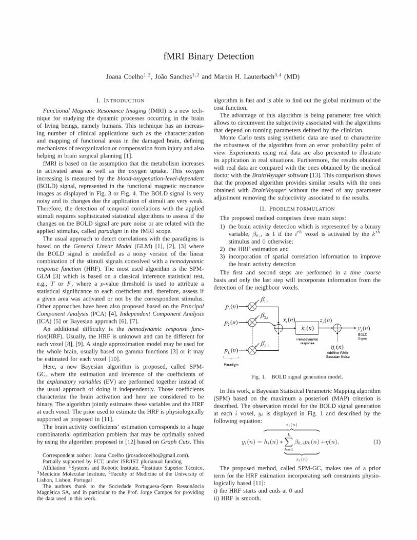
fMRI Binary Detection

Joana Coelho1,2, Joao Sanches1,2 and Martin H. Lauterbach3,4 (MD)

I. INTRODUCTION

Functional Magnetic Resonance Imaging (fMRI) is a new tech-nique for studying the dynamic processes occurring in the brainof living beings, namely humans. This technique has an increas-ing number of clinical applications such as the characterizationand mapping of functional areas in the damaged brain, definingmechanisms of reorganization or compensation from injury and alsohelping in brain surgical planning [1].

fMRI is based on the assumption that the metabolism increasesin activated areas as well as the oxygen uptake. This oxygenincreasing is measured by the blood-oxygenation-level-dependent(BOLD) signal, represented in the functional magnetic resonanceimages as displayed in Fig. 3 or Fig. 4. The BOLD signal is verynoisy and its changes due the application of stimuli are very weak.Therefore, the detection of temporal correlations with the appliedstimuli requires sophisticated statistical algorithms to assess if thechanges on the BOLD signal are pure noise or are related with theapplied stimulus, called paradigm in the fMRI scope.

The usual approach to detect correlations with the paradigms isbased on the General Linear Model (GLM) [1], [2], [3] wherethe BOLD signal is modelled as a noisy version of the linearcombination of the stimuli signals convolved with a hemodynamicresponse function (HRF). The most used algorithm is the SPM-GLM [3] which is based on a classical inference statistical test,e.g., T or F , where a p-value threshold is used to attribute astatistical significance to each coefficient and, therefore, assess ifa given area was activated or not by the correspondent stimulus.Other approaches have been also proposed based on the PrincipalComponent Analysis (PCA) [4], Independent Component Analysis(ICA) [5] or Bayesian approach [6], [7].

An additional difficulty is the hemodynamic response func-tion(HRF). Usually, the HRF is unknown and can be different foreach voxel [8], [9]. A single approximation model may be used forthe whole brain, usually based on gamma functions [3] or it maybe estimated for each voxel [10].

Here, a new Bayesian algorithm is proposed, called SPM-GC, where the estimation and inference of the coefficients ofthe explanatory variables (EV) are performed together instead ofthe usual approach of doing it independently. Those coefficientscharacterize the brain activation and here are considered to bebinary. The algorithm jointly estimates these variables and the HRFat each voxel. The prior used to estimate the HRF is physiologicallysupported as proposed in [11].

The brain activity coefficients’ estimation corresponds to a hugecombinatorial optimization problem that may be optimally solvedby using the algorithm proposed in [12] based on Graph Cuts. This

Correspondent author: Joana Coelho (jrosadocoelho@gmail.com).Partially supported by FCT, under ISR/IST plurianual fundingAffiliation: 1Systems and Robotic Institute, 2Instituto Superior Tecnico,

3Medicine Molecular Institute, 4Faculty of Medicine of the University ofLisbon, Lisbon, Portugal

The authors thank to the Sociedade Portuguesa-Sprm RessonanciaMagnetica SA, and in particular to the Prof. Jorge Campos for providingthe data used in this work.

algorithm is fast and is able to find out the global minimum of thecost function.

The advantage of this algorithm is being parameter free whichallows to circumvent the subjectivity associated with the algorithmsthat depend on tunning parameters defined by the clinician.

Monte Carlo tests using synthetic data are used to characterizethe robustness of the algorithm from an error probability point ofview. Experiments using real data are also presented to illustrateits application in real situations. Furthermore, the results obtainedwith real data are compared with the ones obtained by the medicaldoctor with the BrainVoyager software [13]. This comparison showsthat the proposed algorithm provides similar results with the onesobtained with BrainVoyager without the need of any parameteradjustment removing the subjectivity associated to the results.

II. PROBLEM FORMULATION

The proposed method comprises three main steps:1) the brain activity detection which is represented by a binary

variable, βk,i is 1 if the ith voxel is activated by the kth

stimulus and 0 otherwise;2) the HRF estimation and3) incorporation of spatial correlation information to improve

the brain activity detectionThe first and second steps are performed in a time course

basis and only the last step will incorporate information from thedetection of the neighbour voxels.

Fig. 1. BOLD signal generation model.

In this work, a Bayesian Statistical Parametric Mapping algorithm(SPM) based on the maximum a posteriori (MAP) criterion isdescribed. The observation model for the BOLD signal generationat each i voxel, yi is displayed in Fig. 1 and described by thefollowing equation:

yi(n) =

zi(n)︷ ︸︸ ︷hi(n) ∗

L∑k=1

βk,ipk(n)

︸ ︷︷ ︸xi(n)

+η(n). (1)

The proposed method, called SPM-GC, makes use of a priorterm for the HRF estimation incorporating soft constraints physio-logically based [11]:i) the HRF starts and ends at 0 andii) HRF is smooth.

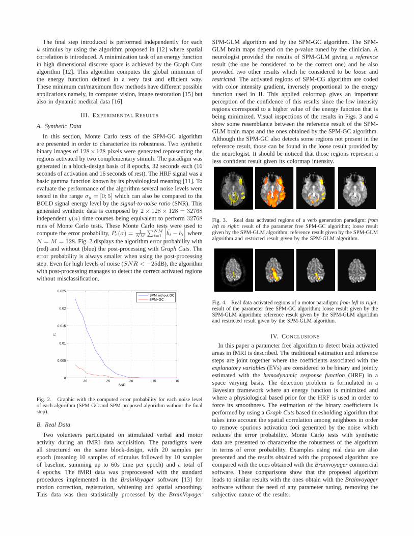
The final step introduced is performed independently for eachk stimulus by using the algorithm proposed in [12] where spatialcorrelation is introduced. A minimization task of an energy functionin high dimensional discrete space is achieved by the Graph Cutsalgorithm [12]. This algorithm computes the global minimum ofthe energy function defined in a very fast and efficient way.These minimum cut/maximum flow methods have different possibleapplications namely, in computer vision, image restoration [15] butalso in dynamic medical data [16].

III. EXPERIMENTAL RESULTS

A. Synthetic Data

In this section, Monte Carlo tests of the SPM-GC algorithmare presented in order to characterize its robustness. Two syntheticbinary images of 128× 128 pixels were generated representing theregions activated by two complementary stimuli. The paradigm wasgenerated in a block-design basis of 8 epochs, 32 seconds each (16seconds of activation and 16 seconds of rest). The HRF signal was abasic gamma function known by its physiological meaning [11]. Toevaluate the performance of the algorithm several noise levels weretested in the range σy = [0; 5] which can also be compared to theBOLD signal energy level by the signal-to-noise ratio (SNR). Thisgenerated synthetic data is composed by 2 × 128 × 128 = 32768independent y(n) time courses being equivalent to perform 32768runs of Monte Carlo tests. These Monte Carlo tests were used tocompute the error probability, Pe(σ) = 1

NM

∑NMi=1

∣∣∣bi − bi

∣∣∣ whereN = M = 128. Fig. 2 displays the algorithm error probability with(red) and without (blue) the post-processing with Graph Cuts. Theerror probability is always smaller when using the post-processingstep. Even for high levels of noise (SNR < −25dB), the algorithmwith post-processing manages to detect the correct activated regionswithout misclassification.

−30 −25 −20 −15 −100

0.005

0.01

0.015

0.02

0.025

SNR

Pe

SPM without GCSPM−GC

Fig. 2. Graphic with the computed error probability for each noise levelof each algorithm (SPM-GC and SPM proposed algorithm without the finalstep).

B. Real Data

Two volunteers participated on stimulated verbal and motoractivity during an fMRI data acquisition. The paradigms wereall structured on the same block-design, with 20 samples perepoch (meaning 10 samples of stimulus followed by 10 samplesof baseline, summing up to 60s time per epoch) and a total of4 epochs. The fMRI data was preprocessed with the standardprocedures implemented in the BrainVoyager software [13] formotion correction, registration, whitening and spatial smoothing.This data was then statistically processed by the BrainVoyager

SPM-GLM algorithm and by the SPM-GC algorithm. The SPM-GLM brain maps depend on the p-value tuned by the clinician. Aneurologist provided the results of SPM-GLM giving a referenceresult (the one he considered to be the correct one) and he alsoprovided two other results which he considered to be loose andrestricted. The activated regions of SPM-CG algorithm are codedwith color intensity gradient, inversely proportional to the energyfunction used in II. This applied colormap gives an importantperception of the confidence of this results since the low intensityregions correspond to a higher value of the energy function that isbeing minimized. Visual inspections of the results in Figs. 3 and 4show some resemblance between the reference result of the SPM-GLM brain maps and the ones obtained by the SPM-GC algorithm.Although the SPM-GC also detects some regions not present in thereference result, those can be found in the loose result provided bythe neurologist. It should be noticed that those regions represent aless confident result given its colormap intensity.

Fig. 3. Real data activated regions of a verb generation paradigm: fromleft to right: result of the parameter free SPM-GC algorithm; loose resultgiven by the SPM-GLM algorithm; reference result given by the SPM-GLMalgorithm and restricted result given by the SPM-GLM algorithm.

Fig. 4. Real data activated regions of a motor paradigm: from left to right:result of the parameter free SPM-GC algorithm; loose result given by theSPM-GLM algorithm; reference result given by the SPM-GLM algorithmand restricted result given by the SPM-GLM algorithm.

IV. CONCLUSIONS

In this paper a parameter free algorithm to detect brain activatedareas in fMRI is described. The traditional estimation and inferencesteps are joint together where the coefficients associated with theexplanatory variables (EVs) are considered to be binary and jointlyestimated with the hemodynamic response function (HRF) in aspace varying basis. The detection problem is formulated in aBayesian framework where an energy function is minimized andwhere a physiological based prior for the HRF is used in order toforce its smoothness. The estimation of the binary coefficients isperformed by using a Graph Cuts based thresholding algorithm thattakes into account the spatial correlation among neighbors in orderto remove spurious activation foci generated by the noise whichreduces the error probability. Monte Carlo tests with syntheticdata are presented to characterize the robustness of the algorithmin terms of error probability. Examples using real data are alsopresented and the results obtained with the proposed algorithm arecompared with the ones obtained with the Brainvoyager commercialsoftware. These comparisons show that the proposed algorithmleads to similar results with the ones obtain with the Brainvoyagersoftware without the need of any parameter tuning, removing thesubjective nature of the results.

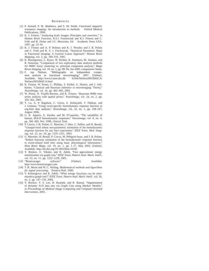
REFERENCES

[1] P. Jezzard, P. M. Matthews, and S. M. Smith, Functional magneticresonance imaging: An introduction to methods. Oxford MedicalPublications, 2006.

[2] K. J. Friston, “Analyzing brain images: Principles and overview,” inHuman Brain Function, R.S.J. Frackowiak and K.J. Friston and C.Frith and R. Dolan and J.C. Mazziotta, Ed. Academic Press USA,1997, pp. 25–41.

[3] K. J. Friston and A. P. Holmes and K. J. Worsley and J. B. Polineand C. Frith and R. S. J. Frackowiak, “Statistical Parametric Mapsin Functional Imaging: A General Linear Approach,” Human BrainMapping, vol. 2, pp. 189–210, 1995.

[4] R. Baumgartner, L. Ryner, W. Richter, R. Summers, M. Jarmasz, andR. Somorjai, “Comparison of two exploratory data analysis methodsfor fMRI: fuzzy clustering vs. principal component analysis,” MagnReson Imaging, vol. 18, no. 1, pp. 89–94, Jan 2000, comparative Study.

[5] F. rup Nielsen, “Bibliography on independent compo-nent analysis in functional neuroimaging,” 2007. [Online].Available: http://www2.imm.dtu.dk/ ˜ fn/bib/Nielsen2001BibICA/Nielsen2001BibICA.html

[6] K. Friston, W. Penny, C. Phillips, S. Kiebel, G. Hinton, and J. Ash-burner, “Classical and Bayesian inference in neuroimaging: Theory,”NeuroImage, vol. 16, pp. 465–483, 2002.

[7] W. Penny, N. Trujillo-Barreto, and K. Friston, “Bayesian fMRI timeseries analysis with spatial priors,” NeuroImage, vol. 24, no. 2, pp.350–362, 2005.

[8] Y. Lu, A. P. Bagshaw, C. Grova, E. Kobayashi, F. Dubeau, andJ. Gotman, “Using voxel-specific hemodynamic response function ineeg-fmri data analysis,” NeuroImage, vol. 32, no. 1, pp. 238–247,August 2006.

[9] G. K. Aguirre, E. Zarahn, and M. D’esposito, “The variability ofhuman, BOLD hemodynamic responses,” Neuroimage, vol. 8, no. 4,pp. 360–369, Nov 1998, clinical Trial.

[10] P. Ciuciu, J.-B. Poline, G. Marrelec, J. Idier, C. Pallier, and H. Benali,“Unsupervised robust non-parametric estimation of the hemodynamicresponse function for any fmri experiment,” IEEE Trans. Med. Imag-ing, vol. 22, no. 10, pp. 1235–1251, 2003.

[11] G. Marrelec, H. Benali, P. Ciuciu, M. Pelegrini-Issac, and J. B. Poline,“Robust bayesian estimation of the hemodynamic response functionin event-related bold fmri using basic physiological information.”Hum Brain Mapp, vol. 19, no. 1, pp. 1–17, May 2003. [Online].Available: http://dx.doi.org/10.1002/hbm.10100

[12] Y. Boykov, O. Veksler, and R. Zabih, “Fast approximate energyminimization via graph cuts,” IEEE Trans. Pattern Anal. Mach. Intell.,vol. 23, no. 11, pp. 1222–1239, 2001.

[13] “Brainvoyager software.” [Online]. Available:http://www.brainvoyager.com/

[14] T. K. Moon and W. C. Stirling, Mathematical methods and algorithmsfor signal processing. Prentice-Hall, 2000.

[15] V. Kolmogorov and R. Zabih, “What energy functions can be mini-mizedvia graph cuts?” IEEE Trans. Pattern Anal. Mach. Intell., vol. 26,no. 2, pp. 147–159, 2004.

[16] Y. Boykov, V. S. Lee, H. Rusinek, and R. Bansal, “Segmentationof dynamic N-D data sets via Graph Cuts using Markov Models,”in Proceedings of Medical Image Computing and Computer-AssistedIntervention, 2001.