ORI GIN AL PA PER

Joint evolution of predator body size and prey-sizepreference

Tineke A. Troost Æ Bob W. Kooi Æ Ulf Dieckmann

Received: 3 June 2005 / Accepted: 3 September 2007� Springer Science+Business Media B.V. 2007

Abstract We studied the joint evolution of predator body size and prey-size preference

based on dynamic energy budget theory. The predators’ demography and their functional

response are based on general eco-physiological principles involving the size of both

predator and prey. While our model can account for qualitatively different predator types by

adjusting parameter values, we mainly focused on ‘true’ predators that kill their prey. The

resulting model explains various empirical observations, such as the triangular distribution

of predator–prey size combinations, the island rule, and the difference in predator–prey size

ratios between filter feeders and raptorial feeders. The model also reveals key factors for the

evolution of predator–prey size ratios. Capture mechanisms turned out to have a large effect

on this ratio, while prey-size availability and competition for resources only help explain

variation in predator size, not variation in predator–prey size ratio. Predation among

predators is identified as an important factor for deviations from the optimal predator–prey

size ratio.

Keywords Body size � Prey-size preference � Size-dependency � Upper triangularity

Introduction

The range of body sizes encountered in nature is enormous. A bacterium with full phys-

iological machinery has a volume of 0.25 9 10-18 m3, while a blue whale has a volume of

up to 135 m3. These body sizes are associated with the different scales in time and space in

which organisms live, and reflect the differences in physiological processes and life his-

tories. A wide range is also found in the prey-size preference of predators: consider, for

T. A. Troost (&) � B. W. KooiFaculty of Earth and Life Sciences, Department of Theoretical Biology, Vrije Universiteit,De Boelelaan 1085, Amsterdam 1081 HV, The Netherlandse-mail: tineke@bio.vu.nl

U. DieckmannEvolution and Ecology Program, International Institute for Applied Systems Analysis, Schlossplatz 1,Laxenburg 2361, Austria

123

Evol EcolDOI 10.1007/s10682-007-9209-1

example, whales feeding on plankton and hyena eating zebra. Like body size, prey-size

preference is an important ecological property, as it determines which trophic links

between predators and prey are established. Together, the body size and the prey-size

preference of predators largely define the structure of a community. While the effects of

body size on individuals and populations has been investigated from many angles (Peters

1983; Kooijman 1986; Yodzis and Innes 1992; Brown et al. 1993), general relationships

between a predator’s body size and its prey-size preference are more difficult to find.

Various mechanisms have been proposed that attempt to explain predator–prey size

ratios and prey-size preferences. These include passive selection mechanisms such as prey

visibility (Rincon and Loboncervia 1995; Svensson 1997) or gape limitation (Rincon and

Loboncervia 1995; Forsman 1996; Mehner et al. 1998; Karpouzi and Stergiou 2003).

Active selection mechanisms, on the other hand, underlie optimal foraging theory, which

assumes that predators select prey sizes that provide the best energy returns. Several

mechanisms based on active selection are discussed in Ellis and Gibson (1997), Manatunge

and Aseada (1998), Rytkonen et al. (1998), Kristiansen et al. (2000), Tureson et al. (2002)

and Husseman et al. (2003). However, since results vary both within and between pred-

ator–prey systems, and the found relationships are highly species-specific, it is difficult to

extract general rules from them.

In recent years, several models have been developed that focus on general large-scale

patterns of feeding links in food webs. Some of these models, such as the cascade model

(Cohen and Newman 1985) and the niche model (Williams and Martinez 2000), are able to

generate food webs that approximate many features observed in real food webs. However,

these models are often descriptive and predator–prey pairs are assigned at random. Other

models do have a more mechanistic basis and include physiological relations based

on body size, but assume a fixed predator–prey size ratio (Loeuille and Loreau 2005).

Aljetlawi et al. (2004) derived a functional response that accounts for both predator and

prey size: the derived relation was sufficiently flexible to be adjusted to many different

specific predator–prey systems. This very flexibility, however, limits the scope for deriving

general rules.

In this study we combine a process-based eco-physiological model with a functional

response that depends on the size of both predator and prey. The model is based on

dynamic energy budget (DEB) theory (Kooijman 2000, 2001), a versatile framework for

modeling metabolic processes with physiological rules for uptake and use of material and

energy. DEB theory does not specify all details of the size-dependence of the functional

response. One of our aims here is to make the terms underlying this functional response

explicit and, where necessary, include additional terms, while staying as close to DEB

theory as possible.

We do not arbitrarily choose predator–prey size ratios, but instead we allow the

predator size and its prey-size preference to evolve independently. The predators are

supplied with prey that have a range of sizes. To keep the analysis feasible, we assume that

the size distribution of prey is constant and does not evolve. The objective is to study

which size combinations between predators and preys are feasible and to which predator–

prey size ratios the considered population or community will eventually evolve. More

specifically, we study how patterns of predator size and prey-size preference depend on

various factors, given a fixed prey-size distribution; the examined factors include envi-

ronmental parameters and ecological parameters, with the latter describing predation as

well as competition. The model focuses on a generalized predator with two life stages, and

therefore is not intended to replace more species-specific studies on size-selective prey

choice. By retaining a general perspective, we hope that the results reported below will

Evol Ecol

123

provide insights into the various factors determining predator–prey size ratios, and thereby

will help understanding of predator–prey size patterns observed in nature.

Model description

Population dynamics

We consider a predator–prey model in which a population of predators feed on one or more

populations of abiotic prey.

The predators are described by one state variable, their biomass density XA (given by

the total amount of structural biovolume per unit of system volume), and by two adaptive

traits, their adult length ‘A and their preference for a prey length ‘P. These two adaptive

traits remain constant throughout an individual’s life, but may change from parent to

offspring through mutation. Prey populations are described by their biomass density Xi, and

consist of organisms of length ‘i, with i = 1,…, n where n is the number of prey popu-

lations. The prey populations are not interacting and are assumed to have a fixed size-

structure. For example, we could consider algal populations grown in a first (illuminated)

chemostat and fed into a second (dark) chemostat where they are consumed by rotifers (see

Kooi and Kooijman 1999).

Our model for the predator is based on a model of a size-structured rotifer population

(Kooi and Kooijman 1997, 1999), of which we use a simplified version that includes only

two life stages for the predator, embryos and adults. Embryos do not feed, but grow by

using the reserves they got from their mothers when eggs were produced. Adults, in

contrast, do not grow but they do feed; the acquired energy is used for maintenance and

egg production. Separating the functions of growth and feeding simplifies the model by

reducing the number of equations. It also removes intraspecific body size scaling relations,

but maintains interspecific scaling relations. These include a size-dependent egg-

production period aA and a size-dependent developmental period ab of the embryo. A

continuous function for reproduction then allows the system to be expressed in terms of

delay differential equations (DDEs). The dynamics of the system can then be described as

follows,

d

dtXiðtÞ ¼ ðXr;i � XiðtÞÞD� IifiðtÞXAðtÞ; ð1aÞ

d

dtXAðtÞ ¼ Rðt � abÞ exp �habð ÞXAðt � abÞ � hXAðtÞ; ð1bÞ

where Xr,i is the incoming density of prey i, fi is the predator’s functional response to prey i(to be further discussed in Section ‘‘Functional responses’’), Ii is the maximum volume-

specific ingestion rate of prey i (which equals the inverse of the handling time [th,i]

multiplied by the probability qs that an attack is successful, Ii = qs/[th,i], where the square

brackets indicate that the handling time is expressed on a volume-specific basis), D is

the dilution rate of prey, and h is the predator’s mortality rate. The delay in reproduction

(t - ab) is due to the predator’s embryo development time ab, which depends on how fast

energy can be mobilized, as described by the specific energy conductance kE, ab = 3/kE

(Kooi and Kooijman 1997). Embryos have the same mortality rate as adults, and the term

exp(-hab) accounts for the mortality of embryos during their development. The predator’s

reproduction rate is given by

Evol Ecol

123

RðtÞ ¼ h

expðhaAðtÞÞ � 1; ð2Þ

(Kooi and Kooijman 1997), which depends on the mortality rate h. Generally, reproduction

rates do not depend directly on adult mortality, but the expression above accounts for the

death of eggs during the egg-production period caused by the mortality of (egg-producing)

mothers. For small mortality rates, the reproduction rate equals the inverse of the egg-

production period, R(t) = 1/aA(t).An expression for aA(t) was derived by Kooi and Kooijman (1997). Their expression is

given by the ratio between the amount of energy needed per egg and the rate with which

energy becomes available for reproduction. The latter depends on the scaled energy density

e of the mother (i.e., on the volume-specific amount of energy [E] divided by the maximum

energy content [Emax]) and on the specific energy conductance kE. At equilibrium, the

scaled energy density e of an adult equals its scaled functional response f, so that the

amount of mobilized energy equals kEf. From this mobilized energy, first the costs of

maintenance have to be paid, calculated by multiplying the maintenance rate coefficient kM

(ratio of costs for maintenance per unit of time to costs for growth) with the energy

investment ratio g (the proportion of the total amount of available energy that is used for

growth). The scaled energy density required to produce an egg depends on the costs for the

structural biomass of a newborn individual and the costs for growth and maintenance

during the embryonic period, gþ ¼ gþ 34

gkM=kE (Kooi and Kooijman 1997), as well as on

the energy density of a newborn individual itself, e: Based on these considerations, the egg-

production period is obtained as

aAðtÞ ¼gþ þ eðtÞ

kEf ðtÞ � kMg; ð3Þ

(Kooi and Kooijman 1997). For a more detailed explanation of the model, including

derivations of ab, R, aA, and g+, readers may want to consult the original work by Kooi and

Kooijman (1997, 1999). All parameters and variables of the model are summarized in

Table 1, with all default parameter values listed in Table 2.

Scaling considerations

Because this study considers adult length to be subject to evolution, some body-size scaling

relations had to be included that were not taken into account in the original model (Kooi

and Kooijman 1997, 1999), where body size was fixed. First, the energy investment ratio gwas no longer assumed to be constant, but instead becomes dependent on body volume

‘3max, following an expression central to DEB theory, g = t/(kM ‘max) (Kooijman 2000).

Note that the adult body size ‘A of the predators is a fixed proportion a of their maximum

size, ‘A = a ‘max. This enables the model to cope with predators that quickly grow to adult

size, without slowing down as would be expected from an asymptotic growth curve.

Second, the specific energy conductance kE is equal to the energy conductance t divided

by the size of the organism, kE = t/‘A. The rationale behind this scaling relation is that

energy is mobilized across membranes, which have a surface area proportional to that of

the organism. As a result, the developmental period of the embryo becomes dependent on

adult body size as well, ab = 3‘A/t. Third, the mortality rate h was assumed to scale with

length, such that larger organisms have a longer life span, h = D‘ref/‘A; at the reference

Evol Ecol

123

length ‘ref mortality rate h is equal to dilution rate D. As such, the dilution rate serves as a

measure for the harshness of the environment.

The scaled energy density of the eggs e is assumed to depend on the scaled energy

density e of the mother. In the original model (Kooi and Kooijman 1997, 1999), a mother

would pass on to her eggs the precise amount of energy such that her offspring, after

development and hatching, would have exactly the same energy density as herself. In this

Table 1 Parameters and state variables of the model

Symbol Dimension Meaning

Physiological parameters

ab, aA T Embryo-development time and egg-production time; ab = 3/kE

e; e – Scaled energy density, of adult and of newborn individuals;e = [E]/[Emax] = f

[E], [Emax], [Emax]ref EL-3 Volume-specific energy density; actual, maximum, and reference

g, g+ – Energy investment ratio for biomass and embryo growth;gþ ¼ gþ 3

4gkM=v

h T-1 Mortality rate

kE T-1 Specific energy conductance; kE = v/‘A

kM T-1 Maintenance rate coefficient

R T-1 Reproduction rate

a – Proportion of the maximum size that is reached; a = ‘A/‘max

t LT-1 Energy conductance

Trophic parameters

b, b0 l3L-3T-1 Volume-specific encounter rate and encounter rate coefficient

D T-1 Dilution rate

f, fi – Functional response; overall, and with respect to prey population i

Ii T-1 Maximum volume-specific intake rate for prey population i

‘i, ‘max, ‘ref L Length of individuals of prey population i; maximum length ofpredator; reference length

tg, tc, th T Ingestion, capture, and handling time

[th], [th,i], [th]ref T Volume-specific handling time: actual, with respect to preypopulation i, and minimum

[tg,0], [tc, 0] T Coefficients for volume-specific ingestion and capture time

Xr,i, Xr,0 L3l-3 Incoming prey density; function, and scaling coefficient

d L Distance between the successive lengths of incoming prey-sizedistribution

l L Mean length of incoming prey-size distribution

rP, r - Standard deviation; of attack probability (niche width), and ofincoming prey-size distribution

qa, qs - Attack probability and capture efficiency

Ecological state variables

XA, Xi L3l-3 Structural volume density of (adult) predators and of preypopulation i

Evolutionary state variables

‘A L Adult length of predator

‘P L Prey-size preference of predator

Dims: T, time; L, length of individual; l, length of reactor; E, energy

Evol Ecol

123

way the mother proportioned the amount of energy per egg, while ensuring that her

offspring would have sufficient energy at the start of its life (right after hatching), at

least as long as the environment did not change in the meanwhile. Also, it implied that

once the system had reached its equilibrium (with respect to prey, predator, and energy

densities), it would remain exactly at this equilibrium (Alver et al. 2006). Here, how-

ever, we study the evolution of prey size-preference, and the offspring may encounter or

prefer different prey sizes than its mother. Therefore, we assume here that a mother takes

into account these uncertainties. She does so by providing her offspring not just with the

amount of energy to end up after hatching with her own energy density [E] she pos-

sesses, but with a larger energy density, ½E�; so that her offspring will always have

sufficient energy densities after hatching, irrespective of the size of its prey. This is

ensured when by scaling the energy density of eggs, not against the mother’s own max-

imum energy density [Emax] (which depends on prey-size availability for her), but against

the maximum possible energy density [Emax]ref. The corresponding scaled energy density eis given by

e ¼ ½E�½Emax�

¼ ½E�½Emax�ref

½Emax�ref

½Emax�¼ ½Emax�ref

½Emax�e: ð4aÞ

If we again use e = f, this can be rewritten as

e ¼ ½Emax�ref

½Emax�e ¼ ½Emax�ref

½Emax�f ¼ ½th�½th�ref

f ; ð4bÞ

where the last step follows from the fact that the maximum energy density is proportional

to the maximum ingestion rate, while the maximum ingestion rate is the inverse of the

handling time, so that [Emax] � 1/[th], (Kooijman 2000, p. 269).

Incoming prey densities

The model introduced above can be analyzed for one or more prey populations. In the latter

case, the incoming prey densities Xr,i were assumed to vary gradually across prey popu-

lations, following a distribution with mean prey size l, (dimensionless) standard deviation

r, and maximum density Xr,0,

Table 2 Default parametervalues

Tildes indicate that parametersare scaled by t, kM and/or Xr,0 tomake them dimensionless

Parameter Default value

~b0 1000

~D 0.1

~‘ref 1

½~tc;0� 3.5

½~tg;0� 0.77

a 0.1

rP 0.05

r 0.25

qs 1

~l 0.5

Evol Ecol

123

Xr;i ¼ Xr;0d

rffiffiffiffiffiffi

2pp exp � 1

2

lnð‘i=lÞ2

r2

!

; ð5Þ

where d denotes the distance between the successive lengths of prey. For numerical pur-

poses, this prey-size distribution was truncated at +3 and at -3 times the standard

deviation r, thus representing 98% of the total distribution. We found that a resolution of

n = 50 was sufficient to ensure that results were essentially unaffected by discretization of

the prey-size distribution.

Functional responses

The sequence of capturing a prey consists of encounter, attack, and handling. These

interactions between predator and prey are assumed to follow a Holling type-II functional

response,

f ¼X

n

i¼1

fi; with fi ¼Xi=Ki

1þPn

j¼1 Xj=Kjand 1=Ki ¼ qa;ibi½th;i�; ð6Þ

where Ki is the half-saturation constant of the functional response to prey i, bi is the

volume-specific encounter rate of the predator with prey i, qa,i is the attack probability for

prey i, and [th,i] is the volume-specific time required for handling prey i. These terms and

their dependencies on the body sizes of both predator and prey, ‘A and ‘i, as well as on the

prey-size preference of the predator, ‘P, are discussed below. In line with DEB theory, we

base these relationships on general scaling principles involving the lengths ‘, surface areas

‘2, or volumes ‘3 of the considered organisms. As a result, the relations derived here are

less detailed than the relations derived by, e.g., Aljetlawi et al. (2004); our assumption

below of fixed scaling exponents also avoids problems with varying dimensions, and thus

interpretations, of scaling coefficients.

Encounter rate b

The encounter rate bi of a predator with a prey of size ‘i arises from encounters within the

predator’s search area. This search area is assumed to be proportional to the predator’s

surface area, b � ‘A2 , as is the case, for instance, for sessile filter feeders that orient their

arms perpendicular to the current. For filter feeders that generate their own current, the

encounter rate equals the filter rate. Their flapping or beating frequency is observed to be

independent of their size (Kooijman 2000), such that the generated current is proportional

to the surface area of their extremities, and thus again to their surface area. Other

organisms may lay in ambush and capture prey that come within reach, i.e., within a

distance that is proportional to the length of a leg or jaw or tongue, such that also here the

encounter rate scales with surface area. Mobile organisms generally move with a speed

proportional to their length: if the width of the path searched for food is proportional to

length, this again leads to an encounter rate that scales with surface area. The encounter

rate also scales with the surface area of the prey ‘i2, as the prey’s visibility or detectability

is assumed to be proportional to the prey cross-sectional area or silhouette. In summary,

we assume bi � ‘A2 ‘i

2. Because the population dynamics above were expressed on a

Evol Ecol

123

per-volume basis, bi is divided by the volumes of predator and prey, leading to the fol-

lowing relationship,

bi ¼ b0

‘2ref

‘A‘i; ð7Þ

where the lengths are measured relative to a reference length ‘ref, so that the encounter rate

coefficient b0, which controls the absolute value of the encounter rate, has the same

dimensions as bi. Without any loss of generality, reference lengths were taken as equal for

predator and prey.

Attack probability qa

The predator prey-size preference ‘P is assumed to evolve separately from the predator’s

adult body size ‘A and is not imposed by morphological constraints such as limited gape

size. Even though such structural limits may exist, we assume here that they are adjusted to

the prey-size preference, rather than vice versa. The probability qa with which a predator

attacks a prey of size ‘i is assumed to be log-normally distributed and depends on the prey-

size preference ‘P and (dimensionless) niche width rP,

qa;i ¼ exp � 1

2

lnð‘i=‘PÞ2

r2P

!

: ð8Þ

On encounter, a prey exactly of the preferred size ‘P will thus be attacked with certainty.

Handling time th

In general, the time required for handling each prey item comprises the time needed for

capture and ingestion.

Ingestion is the process by which the prey is physically taken up into the body of the

predator, passing through, for instance, its outer membrane or its gut wall. First of all,

ingestion time tg is assumed to be proportional to the amount of prey biomass that

has to be ingested, and thus, for one prey individual, proportional to the prey volume,

tg,i � ‘i3.

In addition, for intraspecific comparisons, DEB theory assumes the ingestion time to be

inversely proportional to the surface area through which the intake occurs, and this surface

area is assumed to scale with the total surface area ‘A2 of the predator. For small indi-

viduals, which have a favorable ratio between surface area and volume, the ingestion time

thus is small, while for larger individuals, it is large. In this study, however, we assume all

adult individuals of a population to have the same size, ‘A. For interspecific comparisons,

DEB theory assumes ingestion rates to be proportional to maximum length, ‘max, which

implies that tg � ‘max-1 . Such a scaling may, for instance, be related to gut capacity (body

plan) or diet composition of the predator.

Capture time is assumed to depend on the relative sizes of predator and prey. Larger

prey require a longer capture time because they may be better protected, resist more

strongly, or have to be cut into chunks before being ingested. Specifically, we assume that

the capture time increases faster with prey size than does the corresponding yield, which

Evol Ecol

123

implies that it is proportional to size with an exponent larger than 3; as a default, here, we

assume an exponent of 4, tc � (‘i/‘A)4.

The total handling time th equals the mean length of the handling process, consisting of

capture and ingestion,

th;i ¼ tc;i þ qstg;i

¼ tc;0‘i

‘A

� �4

þqs

tg;0

‘max

‘3i

‘2A

;ð9Þ

where tg,0 and tc,0 are the ingestion and capture coefficients, and qs is the fraction of

attacked prey that is actually captured; only this fraction has to be ingested. As a default,

all attacks are assumed to be successful, qs = 1; the effects of reduced capture efficiencies

are studied in Section ‘‘Evolutionary effects of feeding modes’’.

Because adult size increases with maximum size, and since all adult organisms are

assumed to possess adult size, ‘max can be substituted with ‘A/a. The time th,i that a

predator needs for handling an individual of prey i can be converted into the volume-

specific handling time [th,i], which measures the time that a volume-unit of predator needs

for handling a volume-unit of prey i, through multiplication with (‘A/‘i)3,

½th;i� ¼ ½tc;0�‘i

‘A

þ qsa½tg;0�: ð10Þ

The total handling time [th] given the actual prey-size availability is the sum of prey-

size specific handling times [th,i] weighted with the fraction hi of all attacks that are

directed at prey i,

½th� ¼X

n

i¼1

hi½th;i�; with hi ¼qa;ibiXi

Pnj¼1 qa;jbjXj

: ð11Þ

Finally, [th]ref in Eq. 4b is the absolute minimum, or reference, handling time, which

equals [th,i] at infinitely small prey-sizes, [th]ref = ½th;i�j‘i¼0 = qsa[tg,0], and thus only

depends on predator size.

Choice of units

The model presented above was scaled by maintenance rate kM, energy conductance t, and

incoming prey density coefficient Xr,0. Scaling renders the outcomes independent of these

parameters. The unit of time, T, is chosen as kM-1, the unit of predator and prey length, L, is

chosen as t/kM, and the unit of reactor length, l, is chosen asffiffiffiffiffiffiffi

Xr;03p

kM=u; the latter unit,

however, only features in the dimensions of biomass-volume densities, L3l-3, which are

made dimensionless simply through division by Xr,0.

The remaining variables and parameters, which then become dimensionless, are denoted

by a tilde: for instance, the predator size ‘A (dim: L) was divided by v (dim: LT-1) and

multiplied by kM (dim: T-1) so that the scaled length ~‘A is dimensionless. The scaled

predator and prey densities are indicated by x instead of X, e.g., xA = XA/Xr,0, and the

scaled time t is indicated by s. The default values of the scaled parameters are shown in

Table 2. The scaled model can thus be written as follows,

Evol Ecol

123

dxi

ds¼ ðxr;i � xiÞ ~D� ~IifixAðsÞ; ð12aÞ

dxA

ds¼ ~Rðs� ~abÞ expð�~h~abÞxAðs� ~abÞ � ~hxAðsÞ: ð12bÞ

The scaled reproduction rate ~R is given by

~RðsÞ ¼~h

expð~hðgþ þ eðsÞÞðf ðsÞ=~‘A � gÞ�1Þ � 1; ð13Þ

where f is the functional response, as given in Eq. 6, and e is the scaled energy density of an

egg, as given in Eq. 4. Furthermore, ~D is the scaled dilution rate, ~h ¼ ~D~‘ref=~‘A is the

mortality rate, ~ab ¼ 3 ~‘A is the scaled egg development rate, g is the energy investment

ratio, g ¼ a= ~‘A; and gþ ¼ gþ 34a is the difference in reserve density between the begin-

ning and end of egg development. Note that f, g, and e already were dimensionless

variables before, and are therefore not affected by any choice of units.

Methods

Ecological analysis

The coexistence set is the region in the trait space of the predator’s body size ~‘A and its

prey-size preference ~‘P in which the predator and prey populations can coexist, i.e., where

xi* [ 0 for i = 1,…, n and x*

A [ 0. Here and below, a superscripted asterisk indicates a

population equilibrium, e.g., the scaled reproduction rate at equilibrium is denoted by ~R�:At each point of this trait space there also exists a boundary equilibrium, x*

A = 0 and

x*i = xr,i, which is unstable for trait combinations within the coexistence set and stable for

those outside. In other words, the boundary of the coexistence set is formed by trait

combinations for which the boundary equilibrium changes stability. Consequently, only

within the coexistence set there is a positive equilibrium of the prey–predator system. The

resulting figure (Fig. 1) showing the coexistence set is explained in more detail in Section

‘‘Results/Ecological analysis’’.

We restrict the discussion of the coexistence set to the case in which a single prey

population is supplied to the system. This enables us to check whether a predator can

coexist with prey of a specific size, without this being influenced by the precise choice of

niche width or prey-size distribution. Accordingly, we assume that the prey-size preference

of the predator matches exactly the one available prey size, ~‘P ¼ ~‘1: This cuts short the

evolution of prey-size preference, which will evolve to the size of the available prey

anyway (as this is the only one available). The resulting coexistence set will thus show

which predators can live on which prey. More precisely, the set shows whether a predator

of certain size can coexist with a prey of a certain size when these prey are of the predator’s

preferred size.

An equilibrium point on the boundary of the coexistence set is given by (~‘A; ~‘P ¼ ~‘1) for

which x*1 = xr,1, xA

* = 0, and ~R� expð�~h~abÞ ¼ ~h; where ~R� is the equilibrium value of ~R in

Eq. 13. The remaining points (~‘A; ~‘P ¼ ~‘1) on the boundary of the coexistence set were

then determined by numerically continuating this condition using standard continuation

software.

Evol Ecol

123

Adaptive dynamics theory

For the evolutionary analysis of our model we utilized adaptive dynamics theory, a general

framework that helps investigate phenotypic evolution under frequency-dependent selection

(Dieckmann and Law 1996; Metz et al. 1996; Dieckmann 1997; Geritz et al. 1997). This

approach assumes a time scale separation between the ecological and evolutionary

dynamics, so that mutations in adaptive traits occur sufficiently rarely for the considered

resident population always to be close to its population dynamical equilibrium when probed

by a mutant. Mutants with a positive invasion fitness may replace the resident population. A

series of such replacements leads to phenotypic change of the population. The directions and

endpoints of phenotypic change depend on the selection gradient and are calculated by

means of the so-called canonical equation of adaptive dynamics (Dieckmann and Law

1996). Below we specify, in turn, these general notions for the model analyzed in this study.

Invasion fitness

The invasion fitness of a mutant is defined by its long-term per capita growth rate

rð~‘m;Erð~‘rÞÞ while being rare in the environment Er set by the resident population at its

ecological equilibrium. Here, ~‘ is the vector of the predator’s adaptive traits ~‘ ¼ ð~‘A; ~‘PÞand the subscripts ‘r’ and ‘m’ indicate resident and mutant trait values, respectively. To

calculate the invasion fitness of the mutant we extend Eq. 12 by including the dynamics of

the mutant predator,

dxA;m

ds¼ ~Rmðs� ~ab;mÞ expð�~hm ~ab;mÞxA;mðs� ~abÞ � ~hmxA;mðsÞ: ð14Þ

2

1

32.521.510.50-0.5-1

3

2.5

2

1.5

1

0.5

0

-0.5

-1

Fig. 1 Coexistence set of the investigated predator–prey system. Combinations of scaled predator body size~‘A (vertical) and prey-size preference ~‘P (horizontal) are shown logarithmically, assuming that the preferredprey size equals the one available prey size ð~‘P ¼ ~‘1Þ: The dashed curve depicts the boundary of thiscoexistence set when only ingestion and encounter times are considered, while the continuous curve showsthis boundary when capture times are considered as well. The two arrows indicate the graph’s two possibleinterpretations: (1) the feasible range of predator body sizes for a given prey size, and (2) the feasible rangeof prey-size preferences for a given predator size

Evol Ecol

123

Introducing a mutant in the system also requires a feeding term to be added to Eq. 12a,

as shown in Eq. 21.

As explained in detail in the appendix (Eq. 31), the invasion fitness of the mutant is thus

given by

sð~‘m;~‘rÞ ¼ ~R�m expð�~hm ~ab;mÞ � ~hm; ð15Þ

where ~R�m is the mutant’s reproduction rate at the system’s equilibrium,

~R�m ¼~hm

expð~hmðgþm þ emÞ=ðfm=~‘A;m � gmÞÞ � 1: ð16Þ

Here the functional response fm of the mutant depends on the adaptive traits of both

mutant and resident, because the resident predator sets the environment Er and thus

determines the equilibrium prey density in the system.

Selection gradient

The expected direction of phenotypic change is proportional to the selection gradient, i.e.,

to the derivative of invasion fitness with respect to the adaptive traits of the mutant,

evaluated at the trait values of the resident. For a monomorphic resident population, this

selection gradient is denoted by

rmsð~‘m;~‘rÞ ¼o

o~‘A;m

sð~‘m;~‘rÞ;o

o~‘P;m

sð~‘m;~‘rÞ !

�

�

�

�

�

~‘m¼~‘r

: ð17Þ

Canonical equation

A deterministic approximation of the stochastic evolutionary trajectories of body size and

prey-size preference, jointly driven by mutation and selection, is provided by the canonical

equation of adaptive dynamics (Dieckmann and Law 1996), which for our system is given by

d~‘r

dt¼ qð~‘rÞ

x�A;r~‘3

A;r

rmsð~‘m; ~‘rÞ: ð18Þ

Here q is a compound parameter consisting of the product of the 2 9 2 variance-

covariance matrix of the multivariate mutation distribution (Dieckmann and Law 1996),

the factor 1/2, the mutation probability, and the coefficient of variation of clutch sizes. As

mutations in the two predator traits are assumed to be independent, the variance-covariance

matrix of the mutation distribution is a diagonal matrix. The value of q is irrelevant for this

study as we are only interested in evolutionary equilibria, and not in the timing of the

trajectories leading towards them.

Evolutionary outcomes

Eventually, the population will reach a combination of trait values ~‘r at which the selection

gradient vanishes,

Evol Ecol

123

rmsð~‘m;~‘rÞ ¼ 0: ð19ÞSuch an evolutionary equilibrium may be either stable or unstable according to Eq. 18.

An evolutionary equilibrium may also be situated at a fitness maximum, a fitness mini-

mum, or a fitness saddle according to Eq. 15. In the latter two cases, the evolutionary

equilibrium is not locally evolutionarily stable, so that the resident population may split up

and evolve into two or more sub populations through a process known as evolutionary

branching (Metz et al. 1992, 1996; Geritz 1997, 1998).

Evolutionary analysis

Single-trait evolution

As a preparatory step in the evolutionary analysis of our model, we focus on the

evolution of the predator’s body size. For this purpose we assumed, like in the eco-

logical analysis, that only a single prey population exists and that the predator’s prey-

size preference always matches this prey size, ~‘P ¼ ~‘1: In this case, the evolutionary

dynamics are reduced to the single trait ~‘A: The evolutionary outcome of ~‘A represents the

body size towards which a predator will evolve when feeding on prey of a certain size.

This evolutionary body size was found numerically by integrating the dynamics of ~‘A

according to the canonical equation of adaptive dynamics, Eq. 18, while keeping ~‘P and ~‘1

fixed, until an evolutionary equilibrium was reached. This evolutionary equilibrium was

then determined for a range of prey sizes (and thus prey-size preferences) within the

coexistence set.

Two-trait evolution

The full evolutionary dynamics were studied by allowing the two adaptive traits of the

predator to evolve jointly. In this case, a range of prey sizes was assumed to be available to

the predator according to Eq. 5. The evolutionary equilibrium was again found numeri-

cally, by integrating Eq. 18.

Evolutionary branching

To study the evolutionary process after an evolutionary equilibrium had been reached, an

extended numerical analysis was carried out. This analysis consisted of first integrating Eq.

18 until reaching an evolutionary equilibrium. If this equilibrium was evolutionarily

unstable, i.e., if it corresponded to a fitness minimum or fitness saddle, the original predator

population was equally split into two predator populations and the two corresponding

canonical equations were considered further. The trait values of the two predator popu-

lations were chosen to deviate slightly from that of their ancestor in the two (opposite)

directions of highest fitness increase around the ancestral combination of trait values. The

two canonical equations were integrated, and new predator populations were added

analogously if applicable, until a locally evolutionarily stable evolutionary equilibrium was

reached, corresponding to a fitness maximum in all predator populations. Due to the

Evol Ecol

123

deterministic nature of the adaptive dynamics, more than one predator population may

branch at the same time.

Mutual predation

Finally, to explore the effects of predation among predators, the functional response f was

calculated as the sum of partial functional responses fi, where i now consisted of all prey

populations (i = 1,…, n) as well as of all predator populations (i = n + 1,…, p),

f ¼X

nþp

i¼1

fi: ð20Þ

Stochastic evolution

As a further robustness test, we used a stochastic simulation process instead of the

deterministic dynamics in Eq. 18. Underlying equations were adjusted for multiple prey

populations as discussed at the end of the appendix. We repeatedly integrated the eco-

logical dynamics of the system for 104 time steps, followed by the addition of a new

mutant predator population to the system. The trait values of the mutant were drawn at

random from a normal distribution around the trait values of its ancestor with a standard

deviation of 10-3. The initial biomass of the mutant population was set to a very small

value, xA,m = 10-20. This value was also used as the cutoff biomass density below which a

population was assumed to go extinct. In the case of extinction, the affected population was

removed from the system.

Results

Ecological analysis

We start by studying which predator–prey size combinations can coexist. As explained

above, we restrict the analysis of the coexistence set to the case in which a single prey

population is supplied to the system. For this analysis, the predator’s prey-size preference

equals the single available prey size assumed to be available, ~‘P ¼ ~‘1: The resultant

coexistence set is shown in Fig. 1. This figure can be interpreted in two ways: vertically, as

the feasible range of predator body sizes for a given prey size (illustrated by arrow 1), and

horizontally, as the feasible range of prey-size preferences for a given predator body size

(illustrated by arrow 2).

We separately determined the coexistence set for two different functional responses.

First, only the basic handling processes of encountering and ingesting prey were assumed

to play a role in the functional response of the predator (½~tc;0� ¼ 0; for other parameter

values see Table 2). In this case, Fig. 1 shows that the maximum feasible predator body

size is inversely related to the maximum feasible prey size (dashed line). Second, the

model was extended by including a capture time that depends on the predator–prey size

ratio. Now, large predator–prey size ratios are no longer feasible, and the boundary of the

coexistence set becomes curvilinear (continuous curve).

Evol Ecol

123

Figure 2 shows a set of empirically observed combinations of predator–prey sizes that

were presented by Cohen et al. (1993), together with the coexistence set of our model

based on a size-ratio-dependent capture time (continuous curve). The empirical dataset

consists of 478 size combinations from 30 food webs. In the doubly logarithmic plot, these

are distributed over a triangular area that is bounded above by a maximum predator size,

bounded below by the equality of predator and prey sizes, and bounded on the left by the

minimum prey size. The coexistence sets in Figs. 1 and 2 (continuous curves) are iden-

tical, but for Figure 2 the length variables are translated back from dimensionless

variables into lengths expressed in centimeters. For the two relevant scaling parameters,

kM and t, reasonable values were chosen that lie well within the range of empirically

observed values (kM = 1.44 d-1, t = 0.3 cm d-1; Kooijman 2000); the dilution rate was

adjusted ð ~D ¼ 0:05Þ so as to obtain a slightly better fit for the upper boundary of the

coexistence set.

Evolutionary analysis

After having established which combinations of a predator’s body size and its prey-size

preference are ecologically feasible, we also studied the evolutionary dynamics of these

adaptive traits. Figure 3 again shows the coexistence set (continuous curve) and the

diagonal along which predator size and prey-size preference are equal (dotted line). The

dashed line shows the body size to which the predator will evolve when feeding on a

prey of a given size. In other words, it shows how the evolutionary equilibrium depends

on prey size. This line results from single-trait evolution in ‘A, and applies when only

one prey size is available and ~‘P ¼ ~‘1: The figure shows that the evolved predator size is

positively correlated with prey size, and that the slope of the correlation line is equal to

unity.

P

A

32.521.510.50-0.5-1-1.5

3

2.5

2

1.5

1

0.5

0

-0.5

-1

-1.5

Fig. 2 Comparison of the coexistence set predicted by our model (continuous curve) with empirical datapresented by Cohen et al. (1993). The logarithm of the length of the predator is plotted against the logarithmof the length of the prey, with both lengths being expressed in centimeters. Along the dotted line, body sizesof prey and predator are equal. The dimensionless variables ~‘A and ~‘P were translated back into lengthsusing the two relevant scaling parameters, kM = 1.44 d-1 and t = 0.3 cm d-1; the dilution rate was set to~D ¼ 0:05

Evol Ecol

123

When, instead of one prey size, a range of prey sizes is available simultaneously to the

predator, as described in Section ‘‘Incoming prey densities’’, and both traits are allowed to

evolve jointly, the predator population evolves to an evolutionary equilibrium within the

coexistence set, which in Fig. 3 is denoted by an asterisk.

However, after this evolutionary equilibrium is reached, evolution continues. Since the

evolutionary equilibrium does not correspond to an evolutionarily stable fitness maximum,

the originally monomorphic predator population splits up into two populations and thus

becomes dimorphic. This process of evolutionary branching is repeated several times, such

that the predator population cascades into a range of populations with different trait

combinations, until a locally evolutionarily stable predator community is eventually

reached. In Fig. 3 the trait combinations realized in this evolved community are shown by

filled circles.

Inclusion of predation among predators also leads to sequential evolutionary branching.

The trait combinations resulting under stochastic evolution after 5000 mutations are shown

in as open circles in Fig. 3; at this point in time the system is close to a locally evolu-

tionarily stable equilibrium. The slightly irregular spacing of the realized trait

combinations reflects the stochastic nature of the evolutionary process.

Figure 4 shows how the predator’s body size and prey-size preference at the initial

evolutionary equilibrium (i.e., before the first evolutionary branching) are affected by the

availability of prey sizes. Specifically, the three panels show how the predator’s adaptive

traits vary with three features of the prey: the mean ~l and standard deviation r of the prey-

size distribution, and the prey’s dilution rate ~D: Analogously, Fig. 5 shows the variation of

the predator’s adaptive traits with two features of the predator: its niche width rP and its

probability qs of successfully capturing an attacked prey.

P

A

32.521.510.50-0.5-1

3

2.5

2

1.5

1

0.5

0

-0.5

-1

Fig. 3 Evolutionary outcomes of scaled predator body size ~‘A and prey-size preference ~‘P: The continuouscurve depicts the boundary of the coexistence set, while the dotted line depicts the diagonal along whichpredator size and prey-size preference are equal. The dashed line shows the outcome of single-trait predatorevolution in ~‘A; for a single prey size, with ~‘P ¼ ~‘1: The asterisk indicates the initial evolutionaryequilibrium (and primary evolutionary branching point) of two-trait evolution in the predator whenconsidering a range of available prey sizes. The filled circles show the composition of the predatorcommunity after evolutionary branching (deterministic evolution), while the open circles depict thiscomposition when predation among predators was also taken into account (stochastic evolution)

Evol Ecol

123

Discussion

In the first two subsections below we discuss the results of our ecological analysis,

followed by three subsections of discussion on the results of our evolutionary analysis.

True predators versus parasitic predators

When taking into account only the basic handling processes of encountering and ingesting

of prey, small predator–prey size ratios are feasible (Fig. 1, dashed line). Clearly, this does

not agree with the distribution of empirically observed predator–prey sizes shown in Fig. 2.

However, small size ratios are typically found in parasite-host systems (Memmott et al.

2000), which were not included in the empirical dataset of Cohen et al. (1993). Parasites

are organisms that obtain their nutrients from one or very few host individuals, causing

harm but no (immediate) death. True predators, in contrast, continuously require new prey

a

A,

P

21.510.50

1

0.5

0

-0.5

-1

b

A,

P

0.60.50.40.30.20.10

0.6

0.4

0.2

0

-0.2

-0.4

-0.6

c

A,

P

0.060.050.040.030.020.010

1.5

1

0.5

0

-0.5

Fig. 4 Effects of environmentalparameters on the evolutionaryoutcomes of scaled predator bodysize ~‘A (continuous curve) andprey-size preference ~‘P (dashedcurve). The three panels show theevolutionary equilibrium values(a) for a range of means ~l of theavailable prey-size distribution,(b) for a range of standarddeviations r of this distribution,and (c) for a range of dilutionrates ~D

Evol Ecol

123

individuals, which are killed at attack or quickly thereafter. Because parasites do not have

to overpower their prey, capture times may be neglected. Under these circumstances, our

model predicts that small predator–prey size ratios are feasible, in qualitative agreement

with empirical data.

The transition between parasites and true predators, however, is gradual. This is illus-

trated by the typical classification of a bird-egg eating snake as a predator, while the sea-

cucumber-egg eating pearl fish is classified as a parasite. Examples from the wide range of

parasitic relationships are discussed by Combes (2001). Whatever classification rules are

defined, many exceptions can be found, pointing to the fact that these boundaries are

essentially artificial. DEB theory assumes that predators and parasites are basically of the

same kind, and only differ physiologically. The resulting differences in their parameter

values, however, may lead to considerable, even qualitative, differences in the feasibility of

predator–prey size combinations. In the results of our model, this is reflected by the

qualitative change in the shape of the coexistence set when capture times are considered

(Fig. 1, continuous curve). In this case, the coexistence set is shrunk and it is no longer

feasible for small predators to feed on large prey.

Hence, by adjusting capture times in our model (e.g., by varying the capture time coeffi-

cient), we can account for both parasites and true predators. Similarly, by adjusting other

parameter values, our model may also be expected to account for other types of predators, such

as grazers or parasitoids. As a default, however, we considered a capture time coefficient that

is relatively large, implying that the model mainly corresponds to true predators.

Imperfect upper triangularity

When including in our model a capture time that depends on the predator–prey size ratio,

the feasible set becomes triangularly shaped (Fig. 1, continuous curve), which matches the

a

P

A,

P

0.250.20.150.10.050

0.6

0.5

0.4

0.3

0.2

0.1

0

b

s

A,

P

10.80.60.40.20

2

1.5

1

0.5

0

-0.5

Fig. 5 Effects of ecologicalparameters on the evolutionaryoutcomes of scaled predator bodysize ~‘A (continuous curve) andprey-size preference ~‘P (dashedcurve). The two panels show theevolutionary equilibrium values(a) for a range of niche widths rP

and (b) for a range of captureefficiencies qs

Evol Ecol

123

empirical distribution of observed predator–prey size combinations presented by Cohen

et al. (1993) (Fig. 2). This so-called ‘upper triangularity’ is often found in real food webs

(Warren and Lawton 1987; Cohen at al. 1993, 2003). The term stems from considering a

food web’s matrix of trophic interaction coefficients, in which species are arranged in

hierarchical order, such that all of the non-zero matrix elements lie above the main

diagonal. In the present study, the emergence of upper triangularity implies that larger

predators can feed on a wider range of prey sizes and that for smaller prey sizes, the

feasible range of predator sizes is wider. It also implies that a given species essentially does

not eat other species that are larger than itself, which suggests a body-size-based hierarchy.

Body size has been suggested previously to provide a mechanistic interpretation for the

hierarchy assumption in the cascade model (Cohen and Newman 1985), both by Warren

and Lawton (1987) and by Cohen (1989). However, in our analysis we did not postulate a

size hierarchy as such: instead, this hierarchy naturally emerges from the scaling relations

and size-dependent functional response suggested by DEB theory, and in particular from

the considered proportionality of capture time to predator–prey size ratio.

The value of the capture time coefficient ½~tc;0� considerably affects the shape of the

coexistence set. Yet, when plotted on a doubly logarithmic scale, different values of ½~tc;0�all result in a lower boundary of the coexistence set given by a straight line with slope one,

corresponding to a fixed predator–prey size ratio. Although these lines have different

intercepts, they lie rather close to each other and to the main diagonal for a relatively large

range of values for ½~tc;0�; especially when large predator and prey size ranges are con-

sidered. This finding would explain why, across many natural systems, the distribution of

body size combinations involved in predator–prey links seems to be essentially the same.

Although the predicted boundaries of the coexistence set fit the empirical data rea-

sonably, the fit is not perfect. For example, part of the predicted curvilinear upper boundary

of the coexistence set, corresponding to combinations of small prey sizes with large

predator sizes, is not observed in the considered empirical dataset. Instead, the upper

boundary in the empirical dataset may be described simply by the body size of predators

maxing out at about 150–200 cm. In the model, this curvilinear upper boundary is mainly

determined by the encounter rate between predator and prey being proportional to the

prey’s surface area. Apparently, in natural systems, this is not realistic for large predators

in combination with small prey. Probably, at these size ratios, the prey is not detected by

vision, and the detectability may not be proportional to a prey’s silhouette. This implies

that the model’s fit in this range of size combinations could be improved by including

additional mechanisms. However, we chose to keep our model simple and to stay in line

with DEB theory by including as few additional assumptions as possible.

An interesting property of the model is that the predicted lower boundary of the pre-

dicted coexistence set (Fig. 2, continuous curve) does not coincide with the diagonal along

which predator and prey sizes are equal (dotted line), but instead lies below it (as discussed

above, the exact location of this lower boundary depends on parameter values, and

especially on the capture time coefficient ½~tc;0�). The coexistence set thus extends to pre-

dators feeding on prey individuals that are larger than themselves.

Cohen et al. (1993) found that, in their dataset, approximately 10% of all predators fed

on larger prey. Empirical studies have demonstrated this effect also for other natural food

webs. Because of these consistent observations, the simple cascade model (Cohen and

Newman 1985) has been extended, resulting in the more general niche model (Williams

and Martinez 2000), which is viewed as providing better matches with empirical food web

data (Warren and Lawton 1987; Neubert et al. 2000; Cohen et al. 2003). The proposed

explanations are all based on the assumption that a certain hierarchy exists, but that the

Evol Ecol

123

measures or variables used to characterize it may be imperfect. In contrast, the size-ratio-

dependent capture time assumed in our model provides a mechanism that naturally

explains a body-size-based hierarchy while also allowing for ‘exceptional’ predator–prey

links. This result suggests that not the measures or the variables, but rather the hierarchy

itself is imperfect.

Predator evolution under increased levels of ecological realism

Our approach allows us to study and disentangle the evolutionary effects caused by the

successive incorporation into our model of increased levels of ecological realism. Five

such steps have been taken. First, we started out from a system in which a single predator

adapts to a single prey. Second, we investigated the joint evolution of the body size and

prey-size preference of a single predator confronted with a range of prey sizes. Third, we

considered the adaptive radiation of predator types caused by resource competition. Fourth,

we included trophic interactions among predators to examine their effects on the outcomes

of predator radiation. Fifth, we included evolutionary stochasticity in our model, to cor-

roborate the robustness of our deterministic predictions.

Figure 3 shows that when a single predator adapts to a single prey, predator body size is

positively correlated with prey body size, with a slope equal to 1. This implies that the

predators evolve to a fixed predator–prey size ratio that is constant across predator sizes. A

positive correlation between body sizes of predator and prey is indeed found in vertebrates

(Gittleman 1985; Vezina 1985) and invertebrates (Warren and Lawton 1987), as well as in

planktonic predators (Hansen et al. 1994). Even though these studies underscore that a

general and fixed size ratio does not exist, they do find a constant size ratio within each

trophic or taxonomic group.

When, instead of one prey size, a range of prey sizes is available simultaneously to the

predator, and the body size and prey-size preference of a single predator evolve jointly, the

size ratio at the resultant evolutionary equilibrium (asterisk in Fig. 3) is slightly different

from that resulting from single-trait evolution (dashed line in Fig. 3). This is because now a

range of prey sizes is available, so that the predator’s niche width comes to play a role. The

effects of varying this niche width are discussed in detail in Section ‘‘Evolutionary effects

of feeding modes’’.

Were the range of prey sizes not bounded, the predators would evolve towards ever

smaller body sizes. This is inherent to their physiology, which favors small sizes over large

ones: large organisms have relatively more energy reserves, and therefore a relatively

longer egg-production period, which negatively affects their reproduction rate. Also,

smaller organisms have a relatively large surface area, which is favorable with respect to

the encounter and ingestion rates which both scale with surface area. Apparently, many

physiological mechanisms favor a smaller size. Two factors that, by contrast, may induce

evolution towards larger body sizes are heat loss and environmental variability. The ten-

dency of organisms living at high latitudes to evolve to large body sizes has become known

as Bergmann’s rule (Bergmann 1847; Mayr 1956, 1963), and is often ascribed to the

favorable effects of lower surface-area-to-volume ratios on heat loss. Environmental

variability brings about periods of elevated starvation danger against which a large body

size protects, as larger organisms possess larger energy reserves. These two factors,

however, were not considered in the present study.

Figure 3 (filled circles) shows the trait combinations of the predator populations

that will eventually result from deterministic evolution when adaptive radiations are

Evol Ecol

123

considered. The mechanism underlying the evolutionary branching events is competition

for resources, which leads to disruptive selection. The evolutionary branching process

affects both adaptive traits: under the force of disruptive selection, some populations

evolve towards smaller body sizes and smaller prey-size preferences, while others evolve

to larger body sizes and larger prey-size preferences. When they are isolated, each of the

populations (filled circles) will again evolve towards the first evolutionary equilibrium

(asterisk). The latter may correspond to evolutionary processes on some islands, where

small mammal species have been observed to evolve to a larger size and larger species to

a smaller size. Such a tendency has become known as the ‘island rule’ (Van Valen 1973),

and can thus be understood by the evolutionary dynamics in our model. Figure 3 also

shows that all resulting populations retain the same predator–prey size ratio. From this it

can be concluded that competition for resources may lead to the differentiation of

predator body sizes and prey-size preferences, but not to a differentiation of predator–

prey size ratios.

In determining these evolutionary outcomes, direct interactions among predators, either

through predation or through interference competition, were not taken into account.

Therefore, these outcomes clearly correspond to idealized conditions. Real organisms may

only conform to the resultant predictions in situations in which competition and predation

among predators are naturally absent.

Predation among predators or direct (interference) competition, on the other hand, may

give an additional advantage to large body sizes:larger organisms can be preyed upon by a

smaller range of predators and are thus less vulnerable to predation (as follows from the

triangular distribution of empirical predator–prey combinations), and they may also have

an advantage in the direct competition for food or territory. As such, these processes may

be expected to cause organisms to depart from the predator–prey size ratios predicted

above.

Figure 3 (open circles) shows that predation among predators does indeed lead to much

larger predator–prey size ratios than would be expected on the basis of resource compe-

tition alone. Predation among predators may thus indeed be an important factor for

explaining the large variation of predator–prey size ratios found in nature. Direct (inter-

ference) competition is expected to have a similar effect as predation among predators.

Both factors help explain Cope’s rule (Cope 1896; Benton 2002), which states that natural

selection will tend to produce large-bodied species.

Predictions of deterministic and stochastic renderings of the evolutionary dynamics in

our model agree almost completely, even though the stochastic dynamics expectedly

induce a slight amount of jitter in the evolved predator communities (open circles in

Fig. 3).

Evolutionary effects of environmental factors

Figures 4a and b show how the outcomes of evolution in predator body size and prey-size

preference are affected by the availability of prey sizes. An increase in the mean ~l of the

prey-size distribution causes both traits to increase (Fig. 4a), while the response to vari-

ations in the standard deviation r of the prey-size distribution turns out to be hump-shaped

(Fig. 4b). Although the evolved values of the scaled predator body size ~‘A and prey-size

preference ~‘P change, their ratio remains essentially constant across a large range of the

studied parameter values. Changes in the prey-size distribution, expressed in terms of ~l

Evol Ecol

123

and r, may thus induce shifts in predator body sizes and prey-size preferences, but cannot

explain the variation observed in predator–prey size ratios.

In contrast, an increase in dilution rate does change the evolved size ratio by making it

larger. The evolved body size of predators is affected by the dilution rate through changes

in food abundance: smaller dilution rates reduce both the rate at which new prey enter the

system and the mortality of predators, thus intensifying conspecific competition for

resources. The resulting decrease in evolved predator body size may correspond to the

tendency to dwarfism on islands, which also has been related to limited food resources

(Case 1978).

Evolutionary effects of feeding modes

Ecological factors, such as the predator’s feeding mode, may also affect the evolutionary

outcomes of predator body size and prey-size preference. In particular, a difference

between the predator–prey size ratio of filter feeders and raptorial feeders is seen across

taxonomic groups. Hansen et al. (1994) found that the optimal size ratio of filter feeders is

larger than that of raptorial feeders. They also found that filter feeders generally feed on a

larger range of prey sizes than raptorial feeders. To examine whether the wider prey range

can explain the differences in size ratios, we studied the evolutionary effects of varying the

niche width rP of the predator. Figure 5a shows that the predator–prey size ratio first

increases with niche width and then stabilizes. As the niche width goes to zero, the predator

evolves towards a preference for the smallest prey size that is still available. In this case,

the predator–prey size ratio becomes equal to the size ratio that was predicted from single-

trait evolution; this is expected, as in that analysis the predator was assumed to feed on one

prey size only, which corresponds to vanishing niche width.

Although raptorial feeders may be more size-selective, it is conceivable that they are

also more efficient predators, with a larger fraction of their attacks being successful.

Therefore, we also studied the evolutionary effects of varying the capture efficiency qs.

Figure 5b shows that when a predator is less successful, its body size will become larger,

while its prey-size preference will become smaller. Successful predators will thus evolve

towards smaller predator–prey size ratios. Combining a large niche width with a small

capture efficiency will lead to an even stronger increase in predator–prey size ratio, which

may explain the large size ratio often encountered in filter feeders. These mechanisms

might also provide an explanation for the tendency of the predator–prey size ratio to

decrease with trophic level (Cohen et al. 2003), as predators at higher trophic levels may

more often be raptorial feeders than filter feeders.

Conclusions

A size-dependent functional response was developed and combined with body-size scaling

relationships from DEB theory to establish a physiologically motivated eco-evolutionary

model of adaptations in the body sizes and prey-size preferences of predators. To obtain a

realistic coexistence set for feasible predator–prey size combinations, we included capture

times that depend on predator–prey size ratios. The resulting model exhibits many features,

both ecological and evolutionary, that match empirical observations, such as the triangular

distribution of predator–prey size combinations, the island rule, dwarfing, and the differ-

ence in predator–prey size ratio between filter feeders and raptorial feeders.

Evol Ecol

123

The coexistence set predicted by our model accommodates a wide range of predator–

prey size ratios. By contrast, the evolutionary outcomes in the simplest versions of our

model, in which a single predator adapts either to a single prey or to a range of prey,

imply a fixed predator–prey size ratio. Even though such a fixed size ratio often exists

within trophic and taxonomic groups, it certainly does not apply across these groups. We

therefore introduced and examined various factors that may help explain variation in

predator–prey size ratios. These factors can be organized into three different classes

(Fig. 6).

First, some factors may change the size ratio predicted for single-predator adaptation

(Fig. 6a). Therefore, these factors can have a large impact on observed patterns of

predator–prey size combinations. Examples include changes in physiology and feeding

mode, but also changes in food abundance. Within taxonomic or trophic groups,

organisms often possess a relatively similar physiology, which may therefore explain the

constant size-ratio that is observed within such groups. It should be noted that factors in

this class, in contrast to those listed further below, may also affect the boundaries of the

coexistence set. Yet, on the logarithmic scale used in Figs. 1–3, the resultant lower

boundaries of the coexistence set lie close to each other for a relatively large range of

parameter values.

Second, there are other factors that cause predators to change their body size and prey-

size preference without changing their predator–prey size ratio (Fig. 6b). These include,

for example, changes in the range of available prey sizes. Also, the patterns of size

combinations resulting from resource competition conform to a fixed predator–prey size

ratio. In addition, our analysis has demonstrated that competition for resources induces

differentiation, rather than mere shifts, in predator body sizes and prey-size preferences.

Changes in the available range of prey sizes and resource competition may thus explain the

range of predator body sizes and prey-size preferences observed in nature, but cannot

explain the large variation in predator–prey size ratios.

Third, some factors may systematically induce organisms to depart from the predator–

prey size ratio predicted for single-prey-single-predator adaptation (Fig. 6c). We have

found that predation among predators, as well as interference competition, can cause this

effect, by giving an additional advantage to large body sizes. As such, these processes may

A AA

PPP

Fig. 6 Three different types of change in evolved predator–prey patterns. Continuous curves delineate theboundaries of the coexistence set, dashed lines show the outcomes of single-trait evolution, and asterisksindicate the evolutionary outcome of two-trait predator evolution when a range of prey types is present.Arrows depict changes in the predator’s two adaptive traits ~‘A (vertical) and prey-size preference ~‘P

(horizontal): (a) the expected outcome of evolution in predator body size and predator–prey size ratio ischanged, together with the coexistence set; (b) predator body size evolves, while the predator–prey size ratioremains the same; (c) the predator evolves away from the body size and size ratio predicted by single-traitpredator evolution

Evol Ecol

123

provide an explanation for the tendency of natural selection to produce large-bodied

species (Cope’s rule). Factors from this third class also help us understand the diversity of

predator–prey size ratios encountered in nature.

Distinguishing which of these types of processes is causing the variation in specific

empirical predator–prey size combinations will not be easy. Several parameters and processes

have similar, or compensatory, effects that are difficult to separate, even in experiments. For

example, in most cases it will be problematic to assess the evolutionary outcome of single-

prey-single-predator adaptation. This is because the organism will usually have adapted

evolutionarily to its specific environment, which typically includes predation and competition.

These limitations should be taken into account when trying to explain empirical predator–prey

patterns, or when measuring predator–prey size ratios in experimental setups.

Acknowledgments T. A. Troost thanks the International Institute for Applied Systems Analysis (IIASA)in Austria for providing the possibility of a three-month stay during which the basis for this paper was laidout, and the Netherlands Organization for Scientific Research (NWO) for financing this stay. The authors arevery grateful for the data kindly provided by J. Cohen, S. Pimm, P. Yodzis, and J. Saldana, previouslypublished in Cohen et al. (1993), and for their approval to use them in Fig. 2. We also would like to thankM. Boer, O. Diekmann, F. Kelpin, and M. Kirkilionis for helpful discussions on DDEs. Furthermore, wewould like to thank two anonymous referees for their comments which have considerably improved thepaper. U. Dieckmann gratefully acknowledges financial support by the European Marie Curie ResearchTraining Network FishACE (Fisheries-induced Adaptive Changes in Exploited Stocks), funded by theEuropean Communitys Sixth Framework Programme.

Appendix: Derivation of invasion fitness

In this appendix we show that for determining the invasion fitness of the DDE system

Eq. 12 one can use an ODE formulation without delay. For this purpose, below we derive

the invasion fitness of a mutant predator trying to invade a given resident population of

predators. For determining the coexistence set a formulation without delay can be derived

as well, which we will not demonstrate explicitly, since that derivation is very similar to

the one presented below.

We start from the DDE system Eq. 12, consisting of a prey population x1 and a resident

predator population xA,r, and introduce a mutant predator population xA,m according to Eq.

14. For the sake of clarity, we consider only a single prey population and leave out the

tildes that denote scaled parameters in the main text. The derivation of the invasion fitness

for multiple prey requires just a few adjustments, as is explained at the end of this

appendix. The resulting full system is given by

dx1ðsÞds

¼ xr;1 � x1ðsÞ� �

D� I1;rf1;rðsÞxA;rðsÞ � I1;mf1;mðsÞxA;mðsÞ; ð21aÞ

dxA;rðsÞds

¼ Rrðs� ab;rÞ expð�hrab;rÞxA;rðs� ab;rÞ � hrxA;rðsÞ; ð21bÞ

dxA;mðsÞds

¼ Rmðs� ab;mÞ expð�hmab;mÞxA;mðs� ab;mÞ � hmxA;mðsÞ: ð21cÞ

We assume that there is a stable equilibrium of the prey-resident system, Eq. 21 for

xA,m(s) = 0, at which the resident predator population has positive density. We confirmed

this assumption numerically for the coexistence set shown in Fig. 1 using the default

parameter values given in Table 2.

Evol Ecol

123

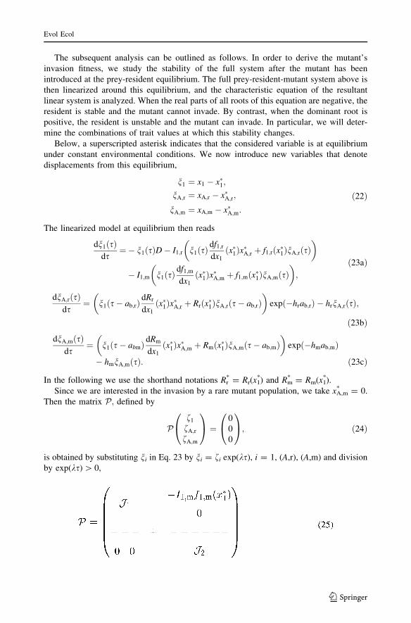
The subsequent analysis can be outlined as follows. In order to derive the mutant’s

invasion fitness, we study the stability of the full system after the mutant has been

introduced at the prey-resident equilibrium. The full prey-resident-mutant system above is

then linearized around this equilibrium, and the characteristic equation of the resultant

linear system is analyzed. When the real parts of all roots of this equation are negative, the

resident is stable and the mutant cannot invade. By contrast, when the dominant root is

positive, the resident is unstable and the mutant can invade. In particular, we will deter-

mine the combinations of trait values at which this stability changes.

Below, a superscripted asterisk indicates that the considered variable is at equilibrium

under constant environmental conditions. We now introduce new variables that denote

displacements from this equilibrium,

n1 ¼ x1 � x�1;

nA;r ¼ xA;r � x�A;r;

nA;m ¼ xA;m � x�A;m:

ð22Þ

The linearized model at equilibrium then reads

dn1ðsÞds

¼� n1ðsÞD� I1;r n1ðsÞdf1;r

dx1

ðx�1Þx�A;r þ f1;rðx�1ÞnA;rðsÞ� �

� I1;m n1ðsÞdf1;m

dx1

ðx�1Þx�A;m þ f1;mðx�1ÞnA;mðsÞ� �

;

ð23aÞ

dnA;rðsÞds

¼ n1ðs� ab;rÞdRr

dx1

ðx�1Þx�A;r þ Rrðx�1ÞnA;rðs� ab;rÞ� �

expð�hrab;rÞ � hrnA;rðsÞ;

ð23bÞ

dnA;mðsÞds

¼ n1ðs� abmÞdRm

dx1

ðx�1Þx�A;m þ Rmðx�1ÞnA;mðs� ab;mÞ� �

expð�hmab;mÞ

� hmnA;mðsÞ: ð23cÞ

In the following we use the shorthand notations Rr* = Rr(x1

*) and Rm* = Rm(x1

*).

Since we are interested in the invasion by a rare mutant population, we take x*A,m = 0.

Then the matrix P; defined by

Pf1

fA;r

fA;m

0

@

1

A ¼0

0

0

0

@

1

A; ð24Þ

is obtained by substituting ni in Eq. 23 by ni = fi exp(ks), i = 1, (A,r), (A,m) and division

by exp(ks) [ 0,

Evol Ecol

123

The 2 9 2 matrix J 1 is given by

J 1 ¼�ðkþ hrÞ � I1;r

dfrdx1

ðx�1Þx�A;r �I1;rf1;rðx�1Þexpð�ðkþ hrÞab;rÞ dRr

dx1

ðx�1Þx�A;r R�r expð�ðkþ hmÞab;rÞ � ðkþ hmÞ

0

@

1

A ð26Þ

and the 1 9 1 matrix J 2 by

J 2 ¼ R�m expð�ðhm þ kÞab;mÞ � ðkþ hmÞ: ð27Þ

The characteristic equation is obtained by the requirement that the determinant of the

matrix P be equal to zero. Then the fi play the role of eigenvector components and the

complex number k plays the role of eigenvalue, which is now a root of the characteristic

equation.

Since the mutant is assumed to be rare, the determinant of P factorizes, being given by

the product of detJ 1 and detJ 2 ¼ J 2; with these two factors corresponding to the two

decoupled systems: the prey-resident system without the mutant (i.e., xA,m* = 0), described

by J 1; and the growth rate of the mutant population, described by J 2:The first factor yields the characteristic equation of the prey-resident system,

detJ 1 ¼ 0: This characteristic equation belongs to the eigenvalue problem for the set of

one ODE and one DDE given by Eq. 23a, without the last term, and Eq. 23b, evaluated at

the equilibrium of the prey-resident system.

The second factor yields the characteristic equation detJ 2 ¼ J 2 ¼ 0 of the first-order

linear homogeneous DDE (Eq. 23c) describing the specific growth rate of the mutant

population. The expression for J 2 in Eq. 27 is of a form discussed extensively by Diek-

mann et al. (1995, p. 312). For this case, the complex roots of the characteristic equation

can be obtained analytically.

The function J 2ðkÞ with k 2 R is monotonically decreasing, dJ 2=dk\ 0: Therefore

there is one unique real root k0. Since J 2ð0Þ ¼ R�m expð�hmab;mÞ � hm; the real eigen-

value equals zero, k0 = 0, if and only if Rm* exp(-hmab,m) = hm. Thus, Eq. 27 has exactly

one positive real solution, k0 [ 0, when Rm* exp(-hmab,m) [ hm and exactly one negative

real solution, k0 \ 0, when Rm* exp(-hmab,m) \ hm. Further, (Driver 1977, p. 321) showed

that equations of this form have infinitely many complex roots. Let kk = lk + ixk; then

substitution of this into the characteristic equation J 2 ¼ 0 and separately equating real

and imaginary parts gives

lk ¼ expð�lkab;mÞR�m expð�hmab;mÞ cosðab;mxkÞ � hm; ð28Þ

xk ¼ � expð�lkab;mÞR�m expð�hmab;mÞ sinðab;mxkÞ: ð29Þ

Clearly, if Eq. 29 holds for xk, it holds also for -xk, so the complex conjugate

kk* = lk - ixk is also a root of the characteristic equation. Furthermore, the unique real

root k0 is the dominant eigenvalue, i.e., the real parts of all other roots are smaller than k0.

This can be seen as follows. Comparison of Eq. 28 with the characteristic equation for k0

gives

k0 � lk ¼ 1� expððk0 � lkÞab;mÞ cosðab;m;xkÞ� �

R�m expð�hmab;mÞ: ð30Þ

Suppose that cos(ab,mxk) = 1, then sin(ab,mxk) = 0, and hence xk = 0, which contradicts

the fact that kk = lk + ixk has non-zero imaginary part. We can thus conclude that

cos(ab,mxk) \ 1. Now assume that k0 - lk B 0, then, with Rm* [ 0 (since Rm

* & Rr* [ 0 due

to small mutational steps), Eq. 30 implies 1 B exp((k0 - lk) ab,m) cos(ab,mxk), and also this

Evol Ecol

123

leads to a contradiction. This shows that Re (kk) \ k0, k = 1, 2,…, or in other words: the real

eigenvalue k0 is the dominant root of the characteristic equation detJ 2 ¼ 0:We had mentioned above that the prey-resident system has a positive stable equilibrium

for the default parameter values given in Table 2. Under these circumstances, the real parts

of the eigenvalues of J 1 are strictly negative. Thus, the dominant eigenvalue k0 of J 2 will

also be the dominant eigenvalue of P; if this k0 exceeds the largest real part of the

eigenvalues of J 1: Hence, for detJ 2 ¼ 0; that is, for Rm* exp(-hmab,m) = hm, the

dominant eigenvalue of P will equal k0 and thus zero. At trait values for which this holds,

the prey-resident-mutant system changes stability, so that the prey-resident system

becomes invadable by the mutant predator.

Now suppose that the real eigenvalue k0 is positive but small. Then the characteristic

equation of J 2 gives

k0 ¼ R�m expð�ðk0 þ hmÞab;mÞ � hm

¼ 1� k0ab;m þ1

2k2

0a2b;m þ � � �

� �

R�m expð�hmab;mÞ � hm;

so that, for k0ab,m � 1, we have

k0 ¼ R�m expð�hmab;mÞ � hm: ð31Þ

Consequently, the rate k0 is the invasion fitness of the mutant predator at the equilibrium

of the prey-resident system, (x1* [ 0, xA,r

* [ 0, xA,m* = 0).

We have thus shown that, if k0ab,m� 1, which holds for small mutational steps, the

invasion fitness can be determined by a formulation without delay, corroborating our

approach in the main text (Eq. 15). The rare mutant (xA,m ? 0) will be able to invade the

stable prey-resident system if and only if Rm* exp(-hmab,m) [ hm. The biological inter-

pretation of this inequality is clear: the mutant’s effective birth rate has to exceed the

dilution rate. After successful invasion, the mutant generally replaces the resident (Geritz

et al. 2002); around evolutionary branching points they can coexist, leading to a dimorphic

predator population (Metz et al. 1992, 1996; Geritz et al. 1997, 1998).

For the (ecological) stability at the boundaries of the coexistence set a formulation

without delay can be derived as well. This derivation is very similar to that of the invasion

fitness explained above, but simpler, as no mutants are considered but only the prey and

resident predator populations. The resulting condition fulfilled at the boundaries of the

coexistence set is given by R*exp(-hab) = h.

Considering multiple prey populations instead of a single one will affect system Eq. 21

in two ways. First, the dynamics of each prey population are described by a separate

equation, such that for n prey populations, the full system will consist of n + 2 equations.

Second, the prey populations will affect the growth rate R (Eq. 13) of the predators (both

residents and mutants) through their functional response f (Eq. 6). The derivation of the

invasion fitness itself, however, is largely analogous to that shown above. The determinant

of the matrix P is still factorizable, and remains given by the product of detJ 1 and detJ 2:J 2 is still given by Eq. 27, adjusted for multiple prey through f in R. J 1 will now be a

(n + 1) 9 (n + 1) matrix, which corresponds to the system of the resident predator and

the n prey populations without the mutant predator. Supported by the simulation results, we

again assume that the system without the mutant is stable. It is then easy to see that the

invasion fitness for multiple prey resembles that for a single prey (Eq. 31), adjusted

through f in R.

Evol Ecol

123

References

Aljetlawi AA, Sparrevik E, Leonardsson K (2004) Prey-predator size-dependent functional response: der-ivation and rescaling to the real world. J Anim Ecol 73(2):239–252

Alver MO, Alfredsen JA, Olsen Y (2006) An individual-based population model for rotifer (Brachionusplicatilis) cultures. Hydrobiologia 560:93–208

Benton MJ (2002) Cope’s rule. In: Pagel M (ed) Encyclopedia of evolution. Oxford University Press,Oxford, pp 185–186

Bergmann C (1847) Uber die Verhaltnisse der Warmeokonomie der Thiere zu ihre Grosse. Gott Stud 3:595–708

Brown JH, Marquet PA, Taper ML (1993) Evolution of body size: consequences of an energetic definitionof fitness. Am Nat 142(4):573–584

Case TJ (1978) Endothermy, and parental care in the terrestrial vertebrates. Am Nat 112(987):861–874Cohen JE (1989) Food webs and community structure. In: Roughgarden J, May RM, Levin SA (eds)

Perspectives on ecological theory. Princeton University Press, Princeton, pp 181–202Cohen JE, Jonsson T, Carpenter SR (2003) Ecological community description using the food web, species

abundance, and body size. Proc Natl Acad Sci USA 100(4):1781–1786Cohen JE, Newman CM (1985) A stochastic theory of community food webs 1. Models and aggregated data.

Proc R Soc Lond B, Biol Sci 224(1237):448–461Cohen JE, Pimm SL, Yodzis P, Saldana J (1993) Body sizes of animal predators and animal prey in food

webs. J Anim Ecol 62(1):67–78Combes C (2001) Parasitism; the ecology and evolution of intimate interactions. University of Chicago

PressCope ED (1896) The primary factors of organic evolution. The Open Court Publishing Company, ChicagoDieckmann U (1997) Can adaptive dynamics invade? Trends Ecol Evol 12(4):128–131Dieckmann U, Law R (1996) The dynamical theory of coevolution: a derivation from stochastic processes.

J Math Biol 34(5–6):579–612Diekmann O, van Gils SA, Verduyn Lunel SM, Walther H-O (1995) Delay equations: functional-, complex-

and nonlinear analysis, Volume 110 of Applied Mathematical Sciences. Springer-Verlag, New YorkDriver RD (1977) Ordinary and delay differential equations, Volume 20 of Applied Mathematical Sciences.

Springer-Verlag, New YorkEllis T, Gibson RN (1997) Predation of 0-group flatfishes by 0-group cod: handling times and size-selection.

Mar Ecol Prog Ser 149(1–3):83–90Forsman A (1996) Body size and net energy gain in gape-limited predators: a model. J Herpetol 30(3):

307–319Geritz SAH, Gyllenberg M, Jacobs FJA, Parvinen K (2002) Invasion dynamics and attractor inheritance.

J Math Biol 44(6):548–560Geritz SAH, Kisdi E, Meszena G, Metz JAJ (1998) Evolutionarily singular strategies and the adaptive

growth and branching of the evolutionary tree. Evol Ecol 12(1):35–57Geritz SAH, Metz JAJ, Kisdi E, Meszena G (1997) Dynamics of adaptation and evolutionary branching.

Phys Rev Lett 78(10):2024–2027Gittleman JL (1985) Carnivore body size: ecological and taxonomic correlates. Oecologia 67(4):540–554Hansen B, Bjornsen PK, Hansen PJ (1994) The size ratio between planktonic predators and their prey.

Limnol Oceanogr 39(2):395–403Husseman JS, Murray DL, Power G, Mack C, Wenger CR, Quigley H (2003) Assessing differential prey

selection patterns between two sympatric large carnivores. Oikos 101(3):591–601Karpouzi V, Stergiou KI (2003) The relationships between mouth size and shape and body length for 18

species of marine fishes and their trophic implications. J Fish Biol 62(6):1353–1365Kooi BW, Kooijman SALM (1997) Population dynamics of rotifers in chemostats. Nonlinear Anal Theory

Meth Appl 30(3):1687–1698Kooi BW, Kooijman SALM (1999) Discrete event versus continuous approach to reproduction in structured

population dynamics. Theor Popul Biol 56(1):91–105Kooijman SALM (1986) Energy budgets can explain body size relations. J Theor Biol 121:269–282Kooijman SALM (2000) Dynamic energy and mass budgets in biological systems. Cambridge University

PressKooijman SALM (2001) Quantitative aspects of metabolic organization; a discussion of concepts. Philos

Trans R Soc B, Biol Sci 356(1407):331–349Kristiansen JN, Fox T, Nachman G (2000) Does size matter? Maximising nutrient and biomass intake by

shoot size selection amongst herbivorous geese. Ardea 88(2):119–125

Evol Ecol

123

Loeuille N, Loreau M (2005) Evolutionary emergence of size-structured food webs. Proc Natl Acad SciUSA 102(16):5761–5766

Manatunge J, Asaeda T (1998) Optimal foraging as the criteria of prey selection by two centrarchid fishes.Hydrobiologica 391(1–3):223–240

Mayr E (1956) Geographical character gradients and climatic adaptation. Evolution 10(1):105–108Mayr E (1963) Animal species and evolution. Harvard University Press, Cambridge, MassMehner T, Plewa M, Hulsmann S, Worischka S (1998) Gape-size dependent feeding of age-0 perch (Perca

fluviatilis) and age-0 zander (Stizostedion lucioperca) on daphnia galeata. Arch Hydrobiol 142(2):191–207

Memmott J, Martinez ND, Cohen JE (2000) Predators, parasitoids and pathogens: species richness, trophicgenerality and body sizes in a natural food web. J Anim Ecol 69(1):1–15

Metz JAJ, Nisbet RM, Geritz SAH (1992) How should we define ‘fitness’ for general ecological scenarios?Trends Ecol Evol 7(6):198–202

Metz JAJ, Geritz SAH, Meszena G, Jacobs FJA, van Heerwaarden JS (1996) Adaptive dynamics: Ageometrical study of the consequences of nearly faithful reproduction. In: van Strien SJ, VerduynLunel SM (eds) Stochastic and spatial structures of dynamical systems. KNAW Verhandelingen,Amsterdam, pp 183–231

Neubert MG, Blumenshine SC, Duplisea DE, Jonsson T, Rashleigh B (2000) Body size and food webstructure: testing the equiprobability assumption of the cascade model. Oecologia 123(2):241–251

Peters RH (1983) The ecological implications of body size. Cambridge University Press, New YorkRincon PA, Loboncervia J (1995) Use of an encounter model to predict size-selective predation by a stream-

dwelling cyprinid. Freshw Biol 33(2):181–191Rytkonen S, Kuokkanen P, Hukkanen M, Huhtala K (1998). Prey selection by sparrowhawks Accipiter nisus

and characteristics of vulnerable prey. Ornis Fenn 75(2):77–87Svensson JE (1997) Fish predation on Eudiaptomus gracilis in relation to clutch size, body size, and sex: A

field experiment. Hydrobiologica 344(1–3):155–161Turesson H, Persson A, Bronmark C (2002) Prey size selection in piscivorous pikeperch (Stizostedion

lucioperca) includes active prey choice. Ecol Freshwa Fish 11(4):223–233Van Valen L (1973). Pattern and the balance of nature. Evol Theory 1:31–49Vezina AF (1985) Empirical relationships between predator and prey size among terrestrial vertebrate

predators. Oecologia 67(4):555–565Warren PH, Lawton JH (1987) Invertebrate predator-prey body size relationships: an explanation for upper

triangular food webs and patterns in food web structure?. Oecologia 74(2):231–235Williams RJ, Martinez ND (2000) Simple rules yield complex food webs. Nature 404(6774):180–183Yodzis P, Innes S (1992) Body size and consumer-resource dynamics. Am Nat 139(6):1151–1175

Evol Ecol

123