A joint initiative of Ludwig-Maximilians University’s Center for Economic Studies and the Ifo Institute

CESifo GmbH · Poschingerstr. 5 · 81679 Munich, GermanyTel.: +49 (0) 89 92 24 - 14 10 · Fax: +49 (0) 89 92 24 - 14 09E-mail: office@CESifo.de · www.CESifo.org

CE

Sifo

Co

nfer

ence

Cen

tre,

Mun

ich

Area Conferences 2013

CESifo Area Conference on

Public Sector Economics11–13 April

Normative Analysis with Societal Constraints

Robin W. Boadway and Nicolas-Guillaume Martineau

Normative Analysis with Societal Constraints

Robin W. Boadway∗ and Nicolas-Guillaume Martineau†

April 2013

Abstract

This paper examines the question of achieving a societal consensus around redistributive

policies. Its extent is measured by the degree of work participation among the different skill

classes that populate the economy. This consensus is driven both by the material incentives

and heterogeneous preferences for leisure of each skill class, and an endogenous social norm,

which embodies societal attitudes towards distributive justice. Results for optimal redistributive

taxation in the presence of an extensive margin of participation show that when a norm is present,

participation taxes are generally lower (resp. higher) than when it is not, whenever it enters as

a benefit or cost for participants (resp. a cost for non-participants). In the event of multiple

participation equilibria, it is examined how changes in the progressivity of taxation may induce

shifts in equilibria. This multiplicity of equilibria is thereafter exploited as a constraint on the

social planner, which views societal consensus as an objective.

JEL classification codes: D63, H21.

Keywords: optimal taxation; societal consensus; social norms; work participation; distributive

justice; redistribution.

1 Introduction

This paper seeks to investigate the importance of achieving a societal consensus surrounding ques-

tions of redistribution. This societal consensus is measured by the extent of co-operative behaviour

in work participation decisions, and rests on social norms which induce work participation above

or below what would result from pure self-interested behaviour. This paper precisely asks what

the presence of such social norms concerning work participation entails for (optimal) redistributive

∗boadwayr@econ.queensu.ca. Department of Economics, Queen’s University. Dunning Hall, 94 University Avenue,Kingston ON K7L 3N6 CANADA. Tel.: +1 613 533-2266. Fax: +1 613 533-6668

†nicolas-guillaume.martineau@usherbrooke.ca. Departement d’economique, Universite de Sherbrooke. 2500, Boule-vard de l’Universite, Sherbrooke QC J1K 2R1 CANADA. Tel.: +1 819 821-8000 ext. 62322. Fax: +1 819 821-7934.We wish to thank Al Slivinsky for commenting on an earlier version of this paper. We also wish to thank semi-nar participants at UQAM, as well as Jean-Guillaume Forand, and various participants at CPEG 2012 – ConcordiaUniversity, all for helpful comments.

1

income taxation, how a social planner’s problem should be conditioned on the prevailing degree of

societal cohesion, and how it can in turn be altered.

It is shown here that the extent of the prevalent societal consensus (i.e., whether the economy

is characterized by a low or a high work participation in equilibrium) matters for a social planner’s

choice of redistributive taxes, its general effect being to constrain the optimal participation tax

rates. Reciprocally, this societal consensus can be fostered or hindered by the social planner’s

choices of redistributive income tax schedules. In that spirit, an engineered shift from a low- to a

high-participation equilibrium (i.e., increasing societal cohesion) can be Pareto-improving, but may

run counter to the social planner’s aversion to inequality and consequent redistributive choices.

Motivating this enquiry is the importance for normative analysis of the social planner’s choice

of objective function and the constraints to which it is subjected. These need to satisfy some basic

characteristics so as to be representative of the individuals’ preferences, and so as to give ade-

quate policy advice. Some characteristics of social welfare functions are innocuous and commonly

assumed, for instance individualism (basing utilities on individuals’ true preferences), anonymity

(treating individuals alike) and the Pareto principle. Yet appropriate policy choices require much

more, especially with regard to questions of redistributive taxation, where interpersonal compar-

isons of utility and their aggregation across individuals particularly matter. Such value judgements

then need to conform with the prevailing social consensus, shaped by the social norms and the

redistributive policies already in place. This societal consensus thus acts as a constraint on the

social planner’s (or party in power’s) choice of policies, but is not immutable for it can in turn be

altered by the implementation of certain policies and through other forms of social engineering.

Underpinning this paper’s definition of societal consensus is co-operative behaviour, which is

fostered or discouraged by a social norm that influences work participation decisions, and that

embodies prevailing societal views of redistributive justice. Seminal work on social norms by Akerlof

(1980) examined how they may drive the wage-setting process, leading to a “fair”wage being chosen

(rather than a market-clearing wage) and involuntary unemployment. Social norms have been

shown to explain deviations from purely rational and self-interested behaviour, for instance in the

context of tax evasion (Gordon, 1989; Myles and Naylor, 1996), and to reconcile theoretical results

with conflicting empirical evidence. They have also recently been shown (Cervellati, Esteban and

Kranich, 2010) to matter in the context of the intensity of labour supply. They can then serve

to explain certain politico-economic attitudes towards redistribution that standard models (e.g.,

Romer, 1975; Meltzer and Richard, 1981) cannot: for instance, how economies with similar initial

income distributions and social preferences may still differ in their chosen levels of redistribution

and their degree of social cohesion, as measured by the individuals’ compliance with the work hours

norm. Such norms concerning the intensity of labour supply were also applied to the context of

optimal income taxation by Aronsson and Sjogren (2010).

In more closely-related work, other authors have invoked social norms to explain the compound-

ing of moral hazard effects caused by the welfare state’s social programs over the long run (Lindbeck,

1995; Lindbeck, Nyberg and Weibull, 1999; Dufwenberg and Lundholm, 2001; Lindbeck, Nyberg

2

and Weibull, 2003). This analysis was done in the context of a reconsideration of the scope and

organization of the welfare state in Europe, following persistently low levels of work participation,

and correspondingly-high levels of benefit claims. This state of affairs was deemed to result from a

weakening of norms – either favouring societal co-operation through moral benefits of participation,

or deterring non-participation through the stigma of receiving social assistance benefits – which fol-

lowed strong adverse macroeconomic shocks having thrown many individuals onto social safety nets

for prolonged periods of time. The present paper differs from previous approaches by examining

the desirability of, and possibility for, societal cohesion and how it interacts a social planner’s (or

party in office’s) social objectives. This analysis is both positive and normative, and makes use of a

broad range of income tax instruments, whereas the work of Lindbeck, Nyberg and Weibull (1999,

2003), for instance, is chiefly characterized by a positive analysis of welfare-state dynamics through

median-voter processes and a linear income tax.

This paper’s norms affecting work participation decisions are also modelled so as to embody

prevailing societal views of distributive justice. These can take two conflicting forms, based upon

seminal works of philosophy (e.g., Rawls, 1971; Nozick, 1974) and found in the recent literature

(e.g., Benabou and Tirole, 2006): either economic outcomes are viewed to be the result of sheer

luck (which justifies redistribution as a means of compensating the worse-off), or are attributed to

effort only (in which case the laissez-faire is optimal). This leads to the derivation of generalized

marginal social welfare weights to the planner’s problem that reflect such views, without them

being embodied in the social welfare function, thus linking this paper to the recent work of Saez

and Stantcheva (2013).

This analysis conducted in the course of this paper yields the following results. First, it is

found that the social norm, when included as an incitement or a deterrent to co-operation affecting

participants, will reduce the optimal participation tax rates relative to the case where it is absent.

Our paper’s model of optimal income taxes and work participation decisions where there is no

social norm corresponds to Saez (2002) (based on the contribution of Diamond, 1980). This result

is attributable to how a change in the tax incentives to participate is compounded by the presence

of the social norm, which makes participation more volatile – thus amplifying the budgetary loss of

increasing redistribution to non-participants, while also calling for less of it, for lower numbers of

non-participants increase the welfare of participants. This does not however necessarily hold when

the social norm enters as a cost for non-participants. A higher participation tax may result than in

the case without a social norm if the planner sufficiently cares about the welfare of non-participants,

and the feedback effects of the social norm on participation and budgetary balance are relatively

mild.

It is also investigated how the social norm can lead to the existence of multiple locally-stable

equilibria in work participation. Transitions between high- and low-participation equilibria can be

induced by changes in the income tax schedule. Conditions for the Pareto-dominance of a high-

participation equilibrium over its low-participation counterpart are also derived, and are shown

to constrain the choices of a social planner engineering a transition from the latter to the former

3

equilibrium, by reducing the prevailing extent of redistribution compared with (unconstrained)

optimal tax problem.

The paper is organized as follows. Section 2 first defines individual preferences, the nature of

the social norm, and how they jointly determine individual work participation decisions. It also

examines how the social norm may lead to a single equilibrium or multiple locally-stable equilibria

in work participation. Section 3 then considers the optimal redistribution problem of a “naıve” or

myopic social planner, that is one not explicitly considering the potential multiplicity in equilibria

when solving for the optimal tax structure. The next section (Section 4) generally considers the

issue of the incentives provided by the welfare state through a redistributive income tax, their

interaction with a social norm concerning work participation, and how they may lead to different

levels of societal co-operation and equilibria in work participation. It finally considers the question

of transitions from low- to high-participation equilibria, and how socially engineering them through

material incentives may conflict with the social planner’s objective. Finally, Section 5 concludes

this paper with a summary and a discussion of its results.

2 Labour market participation, social norms, and optimal redis-

tribution

We consider how social norms concerning work-force participation interact with the implementation

of a certain redistributive taxation schedule. In effect, the compliance of the population with the

endogenous social norm determines the extent of redistribution possible, and the potential need

for taxation policy to trigger a shift in participation. To study this issue transparently, we adopt

the pure extensive labour supply model of Diamond (1980) and Saez (2002). It is augmented with

a social norm, either in the form of an inducement or deterrent to participate, which respectively

mitigates or amplifies the extent to which a productive individual may choose to remain idle instead

of working, out of self-interested behaviour.

Let there be a population, normalized to be of size 1, composed of I + 1 skill classes denoted

by i = 0, 1 . . . , I, each of natural population ni (that is to say, the population endowed with a

certain skill set). Contrast this with the effective population of each class, denoted by hi, which

results from the work participation decisions of its individual members. With each of these skill

classes is associated an exogenous income wi, identical for all working members of a given skill,

and preferences for leisure that are heterogeneous both within a skill class and between classes.

The participation decision of an individual in any given class but class 0 (who is deemed to be

inactive) therefore hinges jointly on preferences for leisure and the social norm, both of which will

be explicitly described later. The number of non-participants, h0 = 1 −∑i �=0 hi, includes persons

of all skill levels who choose not to participate.

The next subsections are as follows. First, the participation decision, and how the social norm

enters it are explained at length. Second, the impact of the social norm on the work participation

elasticity of each skill group is considered. Third, we investigate the existence and stability condi-

4

tions for there to be an equilibrium (or many equilibria) in participation for a given tax schedule,

a distribution of preferences for leisure, and the norm. Finally, the social planning problem for a

redistributive taxation schedule is solved, and the results are compared with the canonical Saez

(2002) optimal taxation formula in the presence of an extensive margin of participation only.

2.1 The participation decision: preferences for leisure and the social norm

We first describe the participation decision, which will be useful for characterizing the optimal tax

problem, and in so doing we specify functional forms for utility and the social norm.

2.1.1 Characterizing preferences

Assume a certain distribution of leisure preferences in each skill class i, with utility being quasi-

linear in consumption so as to abstract from income effects. Let vi be the utility of leisure for a

person with skill level i, where vi is stochastic and follows the distribution Γi(vi). An individual in

class i with utility of leisure vi will participate in the labour force if:

ci + x(h0, c0) ≥ c0 + vi

where x(h0, c0) is the co-operative incitement (or deterrent) to participate, which depends on the

total number of non-participants of all types1 and the level of transfers accruing to them. The

function x(·, ·) is assumed to be the same for all individuals and to embody a certain societal view

of distributive justice, which affects one’s moral inclination to participate in the work force. We

consider two diametrically opposed cases: the first, where economic outcomes are attributed to luck;

and the second, when they are attributed to effort.

The social norm when economic outcomes are attributed to luck In the case of economic

outcomes being attributed to luck, the function x(·, ·) has the following properties:

x(h0, c0) ≥ 0 ∀(h0, c0)xh ≡ ∂x

∂h0< 0

xc ≡ ∂x

∂c0> 0 ∀c0 < c0 (1)

< 0 otherwise

xch ≡ ∂2x

∂h0∂c0> 0 ∀c0 < c0

< 0 otherwise.

1The function’s argument is here the number of non-participating individuals, but it could very well be re-writtenas a function of participating individuals: x(1−∑

i �=0 hi, c0), where as mentioned hi is the effective population of skillclass i.

5

A positive moral benefit (i.e., a co-operative incitement to participate) could thus only be present

for a certain range of h0 ∈ [0, h0], where for all h0 > h0, x(h0, c0) = 0, and purely self-interested

behaviour once again prevails. The final cross-partial derivative (for which Young’s theorem holds,

the function x being continuous) states that non-participation and transfers to the idle are com-

plements, for all c0 < c0, where c0 is some threshold level of transfers to the idle. An increase in

the transfers to non-participants translates into an increase in the marginal moral benefit (or, more

accurately, a decrease in the marginal moral cost) of seeing more members of class 0. Reciprocally,

for a given level of transfers, an increase in h0 increases the marginal moral benefit of redistributing

to the idle.

The moral benefits accruing to participants are positive and increasing in c0, and non-participation

and transfers are complements2: jointly, this evokes the view that non-participants are not respon-

sible for their fate. Meanwhile, the function x(·, ·) reflects the fact that the norm morally rewards

conformism: the moral benefits of participation are decreasing in the number of non-participants.

Yet they decrease at a slower rate when c0 increases, due the moral benefit of not stigmatizing

non-participants for their fate, and redistributing income towards them.

The social norm when economic outcomes are attributed to effort In the case of economic

outcomes being attributed to effort, the function x(·, ·) takes the following form:

x(h0, c0) = 0 for c0 = 0 or h0 = 0

< 0 otherwise

xh ≡ ∂x

∂h0< 0

xc ≡ ∂x

∂c0< 0 ∀c0 (2)

xch ≡ ∂2x

∂h0∂c0< 0 ∀c0.

Note here that the function takes non-positive values, rather than non-negative ones. It therefore

acts as a moral cost of participation, or a“co-operative”deterrent to participate: the sight of idleness,

attributed to a lack of effort, weakens the resolve of participants to work and fund transfers to non-

participants. Its effect is therefore to lower participation below the self-interest benchmark. Also

noteworthy is the complementarity3 between idleness and the level of transfers, which signifies that

for participants, the marginal moral cost of idleness (xh) increases as transfers (c0) increase, and

that the marginal moral cost of transfers to the idle increases the more non-participants there are.

2Note however that whenever transfers are above some threshold c0, the complementarity relationship then becomesone of substitutability : increasing transfers to the idle decreases the marginal moral benefit (increases the marginalmoral cost) of seeing more members of class 0, while increasing h0 further decreases the moral benefit of redistributingto the idle.

3The negative cross partial derivative xch here represents complementarity, due to the function and both partialderivatives xh and xc taking negative values: an increase in transfers to non-participants increases the marginal moralcost caused by their numbers (i.e., makes xh more negative), while an increase in their numbers increases the marginalmoral cost caused by transfers (i.e., makes xc more negative).

6

Another, starker way of modelling economic outcomes being attributed to effort is for the moral

cost to affect non-participants instead: this reflects the stigma incurred by those who do not work,

as a result of societal attitudes towards idleness. In such a case, the utility of participants in class

i would be ci + vi, and that of non-participants from class i, c0 + vi + x(h0, c0). The function x(·, ·)then has the same properties as stated in (2) (including xc < 0 : the stigma increases as c0 does),

except that now xh > 0 (more non-participants decreases stigma, and makes x(·, ·) less negative;

however, increasing c0 decreases the positive marginal effect of an increase in h0 on stigma, hence

it is still that xch < 0), but its effect is to increase participation above self-interested levels, as in

the case of outcomes being attributed to luck. (Note that there does not exist an analogous way of

modelling the norm as a moral cost to non-participants when outcomes are attributed to luck, as

there should then be no such stigma befalling them.)

In what follows, we chiefly focus on the norm affecting participants, but still allow for a norm

affecting non-participants wherever it leads to different results.

Effective skill class populations The cut-off individual in each skill class i is the person who

is indifferent between working and being idle. Let vi be his preference for leisure, which satisfies:

ci + x (h0, c0) = c0 + vi

⇐⇒ vi = ci − c0 + x (h0, c0)

regardless of how the norm is modelled, as long as it affects participants.4 Thus, if the natural

population of each skill class is given by ni, with∑I

i=0 ni = 1, then hi, the effective population of

class i, is then:

hi(ci − c0 + x(h0, c0)) = niΓi(ci − c0 + x(h0, c0)) ∀i > 0

h0 = n0 +∑i �=0

ni (1− Γi(ci − c0 + x(h0, c0)))

= 1−∑i �=0

niΓi(ci − c0 + x(h0, c0))

Having fully characterized the participation decisions of each class and the preferences underlying

it, let us turn to how the social norm impacts the elasticity of participation of each skill class.

4If it affects non-participants, we have instead:

ci = c0 + vi + x(h0, c0)

and thus:

hi(ci − c0 − x(h0, c0)) = niΓi(ci − c0 − x(h0, c0)) ∀i > 0

h0 = n0 +∑i �=0

ni (1− Γi(ci − c0 − x(h0, c0))) .

7

2.2 The impact of a social norm on the elasticity of participation

In the absence of a social norm determining the extent of societal co-operation, the number of

participants of skill class i can be represented by: hi(ci− c0), with h′i(ci− c0) > 0, hi > 0 ∀ci− c0 >

0, and hi = 0 ∀ci − c0 ≤ 0.

In keeping with the previous subsection, let us augment this by making participation a function

of h0, the inactive portion of the population, so that the number of type-i participants is hi(ci −c0 + x(h0, c0)), where:

∂hi∂h0

= h′i(ci − c0 + x(h0, c0))xh < 0 ∀i = 0.

Since total population is normalized to be 1, that means in turn:

h0 = 1− hi(ci − c0 + x(h0, c0))−∑j �=0,i

hj(cj − c0 + x(h0, c0)) (3)

which implies:dh0dh0

=∂h0∂h0

= −∑i �=0

h′i(ci − c0 + x(h0, c0))xh

and:

∂2h0∂h20

= −⎛⎝∑

i �=0

h′′i (ci − c0 + x(h0, c0))xh +∑i �=0

h′i(ci − c0 + x(h0, c0))xhh

⎞⎠ .

The elasticity of participation in the absence of a norm is generally defined thus:

ηi ≡ ci − c0hi

dhid(ci − c0)

=ci − c0

hi(ci − c0)h′i(ci − c0)

which depends only on ci − c0.

Yet in the presence of a social norm, the elasticity of participation depends not only on the

direct reward from participating ci − c0, but also on the total number of non-participants h0, and

the absolute level of c0. The total effect of a change in ci − c0 feeds back into h0, first by the direct

effect of a change in the participation of group i, and second, by a change in the participation of

all other groups, which in turns affects h0, etc. The system’s stability is by no means guaranteed:

following a small disturbance, it could spiral up to (near) full participation for all members of all

groups except of those of skill 0, or down to minimal participation.

Putting these concerns aside for the moment (the next subsection considers them at length), the

new elasticity measure can be written:

ξi =ci − c0hi

dhid(ci − c0)

=ci − c0hi

(h′i + h′ixh

dh0d(ci − c0)

)(4)

by the chain rule, keeping here c0 constant for simplicity.5 Note that since h0 is a function of all hj5Not doing so would only add an extra term to the above equation, −((ci − c0)/hi)(h

′ixcdh0/d(ci − c0)), without

8

(including hi, which depends on ci − c0), which are in turn functions of h0, it follows from (3) that:

dh0d(ci − c0)

= − dhid(ci − c0)

−∑j �=0,i

h′jxhdh0

d(ci − c0)

⇐⇒ dh0d(ci − c0)

= − dhid(ci − c0)

1

1 +∑

j �=0,i h′jxh

≡ − dhid(ci − c0)

1

1 +Ai. (5)

Since an increase in ci − c0 should increase hi and decrease h0 – thereby making the left-hand side

of equation 5 negative, and first term of its right-hand side positive – the second term on the right-

hand side, (1 + Ai)−1, must be positive, which implies that Ai =

∑j �=0,i h

′jxh > −1. Interestingly,

(5) can be rewritten as:

1

1 +Ai= −dh0

dhi. (6)

Combining (5) with (4) yields:

dhid(ci − c0)

= h′i

(1 +

∑j �=0,i h

′jxh

1 +∑I

j=1 h′jxh

). (7)

Since h′jxh < 0 ∀j = 0 (less participation breeds less participation, either by decreasing the moral

benefit or cost of participation, or by lowering the stigma attached to receiving transfers), we have

that:

1 +∑

j �=0,i h′jxh

1 +∑I

j=1 h′jxh

> 1 sodhi

d(ci − c0)> h′i =

∂hi∂(ci − c0)

. (8)

Participation is thus more responsive following infinitesimal changes in consumption bundles with

the addition of the social norm than without, where the total derivative would then be equal to the

partial derivative. This is expected, due to feedback effects on participation.

What about the elasticity of participation, then? When outcomes are attributed to luck, or when

the norm enters as a moral cost for non-participants, it increases each group,s participation relative

to the self-interest benchmark. Yet, by the argument outlined above in mathematical terms, it also

increases the responsiveness of each group’s participation following changes in relative consumption

bundles. Comparing elasticities of participation therefore leads to ambiguous results, since for a

given tax-and-transfer scheme denoted by ci − c0 ∀i = 0, and for x(h0, c0) > 0:

hi(ci − c0 + x(h0, c0)) > hi (ci − c0)

while, by virtue of the above discussion, it was shown that:

dhi(ci − c0 + x(h0, c0))

d (ci − c0)>

∂hi(ci − c0 + x(h0, c0))

∂ (ci − c0)=

dhi (ci − c0)

d (ci − c0)

changing the overall characteristics of the newly-found elasticity function.

9

which implies:

ξi =ci − c0

hi(ci − c0 + x(h0, c0))

dhi(ci − c0 + x(h0, c0))

d (ci − c0)≷ ci − c0

hi (ci − c0)

dhi (ci − c0)

d (ci − c0)= ηi.

The only exception to this occurs when the norm embodies the view that outcomes are attributed

to effort, and it enters the utility of participants as a moral cost. Since participation is depressed

relative to the self-interest benchmark, it is now that ξi > ηi.

Let us now turn to the determination of (stable) equilibrium levels of participation induced by

the social norm.

2.3 Equilibrium participation and the social norm

In this subsection, we consider conditions necessary and sufficient for the social norm to lead to

at least one stable equilibrium in participation. Though we characterize them explicitly only for a

norm affecting participants, the same conditions hold when it affects non-participants instead.

The equilibrium resulting from the social norm (i.e., h0, the number of inactive individuals) is

the solution of the following fixed-point equation:

h0 = 1−∑i �=0

hi(ci − c0 + x(h0, c0))

This fixed-point equation may have no solutions, a single solution, or multiple solutions, each of

which can be locally stable or not. We consider under what conditions such scenarios are foreseeable,

and which ones may be particularly interesting for further consideration: namely, the cases where

there can be (at least) two locally-stable equilibria, one characterized by low participation (a “bad”

or “vicious” equilibrium), and another by high participation (a “good” or “virtuous” equilibrium).

Note first that the right-hand side of the above equation is an increasing function of h0, and so

is its left-hand side. Consider the case where h0 = n0, the number of type-0 persons, so all persons

with skills i > 0 fully participate. It is therefore plain to see that a stable equilibrium will exist

provided that the right-hand-side, when evaluated at n0, exceeds n0, and that its slope is less than 1.

More formally, the above equation represents a generally non-linear, first-order difference equation

in h0, which can be represented by a phase diagram. Re-write it as follows for added clarity:

h+0 = 1−∑i �=0

hi(ci − c0 + x(h0, c0))

where the superscript “+” denotes the temporally subsequent value, when iterating.

This function maps from A = [n0, 1] to itself. One may here invoke Brouwer’s fixed point theo-

rem, since the function h0 = f(h0) is assumed to be continuous (and if it were assumed otherwise,

Tarsky’s fixed point theorem could still be used). Brouwer’s theorem states that for the continuous

function to have a fixed point, the set A must be compact, convex and non-empty. That interval of

the real line satisfies all three conditions. Therefore, there exists a fixed point (which may, or may

10

not, be unique). It is an interior solution provided that the function cross the 45-degree line, and a

corner solution (n0 or 1) if it happens to be completely below or above it, respectively.

Local stability of a steady-state equilibrium h�0 requires that:

∣∣∣∣dh+0 (h�0)dh0

∣∣∣∣ =

∣∣∣∣∣∣−∑i �=0

h′i(ci − c0 + x(h�0, c0))xh(h�0, c0)

∣∣∣∣∣∣ < 1

⇐⇒∑i �=0

h′i(ci − c0 + x(h�0, c0))xh(h�0, c0) > −1

since each h′ixh is non-positive for the whole range of h0. Furthermore, given that −∑i �=0 h

′ixh > 0,

convergence towards a steady state will occur monotonically.

Participation hinges on two parameters: preferences for leisure, and the social norm itself (more

precisely, the moral (dis)incentive to participate, captured by x(h0, c0)). The number of participants

of skill-type i, i > 0 is given by hi = niΓi(ci−c0+x(h0, c0)), and the total number of non-participants

is h0 = n0 +∑

i �=0 ni(1− Γi(ci − c0 + x(h0, c0))). It is therefore the case that:

∂hi∂h0

= h′i (·)xh(h0, c0) = niΓ′i (·)xh(h0, c0) ∀i = 0

and:

∂2hi∂h20

= h′′i (·)xh(h0, c0) + h′i (·)xhh(h0, c0) = niΓ′′i (·)xh(h0, c0) + niΓ

′i (·)xhh(h0, c0) ∀i = 0

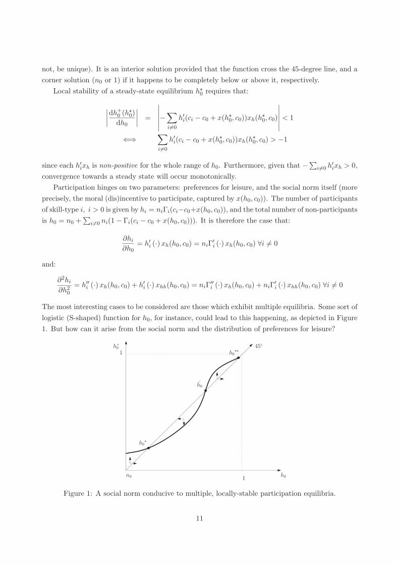
The most interesting cases to be considered are those which exhibit multiple equilibria. Some sort of

logistic (S-shaped) function for h0, for instance, could lead to this happening, as depicted in Figure

1. But how can it arise from the social norm and the distribution of preferences for leisure?

n0 h01

145◦

h0�

h0��

h0

h+0

Figure 1: A social norm conducive to multiple, locally-stable participation equilibria.

11

Let us focus on the characteristics of the social norm by assuming a particular distribution of

leisure preferences for each class: namely, that it is uniformly distributed with a certain mean and

variance. Denote therefore the probability density function (p.d.f.) for class i as:

Γ′i(vi) = γi(vi) =

⎧⎨⎩

1bi−ai

∀vi ∈ [ai, bi]

0 otherwise

It follows that:

∂hi∂h0

= h′ixh =ni

bi − aixh(h0, c0) ∀i = 0 and

∂2hi∂h20

= h′′i xh + h′ixhh =ni

bi − aixhh(h0, c0) ∀i = 0

The slope of equation h+0 = 1−∑i �=0 hi(ci − c0 + x(h0, c0)) therefore becomes:

dh+0dh0

=∑i �=0

ni

bi − aixh(h0, c0)

while its second derivative is then:

d2h+0dh20

=∑i �=0

ni

bi − aixhh(h0, c0) (9)

Thus, for this function to have two different segments leading to locally-stable equilibria, the second

derivative xhh in equation 9 must change signs. It must therefore be the case that x(h0, c0) is first

decreasing at an increasing rate (its second partial derivative is negative, and the first-difference

equation is therefore increasing and convex in h0 – both its first and second partial derivatives are

positive), then past an inflection point h0, x(h0, c0) is decreasing at a decreasing rate (its second

partial derivative is positive, and the first-difference equation is therefore increasing and concave in

h0 – its second derivative is negative, while its first derivative is positive). For h0 to be unstable,

it must not be a saddle point, which means that xh(h0, c0) < 0, as is already the case for all other

h0 ∈ [n0, 1].

Having established the conditions necessary and sufficient for a locally-stable equilibrium in

labour force participation to exist, let us now turn to the determination of optimal redistributive

taxation in the presence of such a social norm.

3 The basic optimal redistribution problem in the presence of a

social norm

We characterize the optimal redistributive tax-and-transfer scheme in the presence of a social norm

by assuming that the social planner not only takes into account the behavioural responses of indi-

viduals induced by the social norm, but also includes the moral benefit (or cost) of participation

in its measure of social welfare. In doing so, the social planner both reflects the individuals’ pref-

12

erences, and fully internalizes the norm’s effects on redistribution and welfare. The social planner

here sets and announces the optimal tax schedule first, anticipating the participation decisions of

individuals. They choose whether to be active next, based on their observed tax burden relative to

that of non-participants.

Note however that the planner is here either naıve or myopic as to the exact shape of the social

norm function, and the possible multiplicity of equilibria. So rather than conditioning its problem

on being in a given participation equilibrium, brought upon by the laissez-faire or a certain tax

schedule, it conducts itself as though it were irrelevant or the equilibrium were unique. Effectively,

this is equivalent to finding a local maximum, rather than choosing the global maximum. This

approach will show its obvious limits when multiple equilibria are considered, in the next section.

3.1 The social norm as a moral inducement or deterrent to participate: out-

comes being attributed to luck or effort

Let u(ci+x(h0, c0)) and u(c0+vmi ) be the social utilities of type-i’s when working and not working.

The social utility functions are concave, and the degree of concavity reflects the planner’s aversion

to inequality. The planner’s problem can be written, using j instead of i as a subscript in the sums:

max{c0,··· ,cI}

∑j>0

hj(cj − c0 + x(h0, c0))u(cj + x(h0, c0)) +∑j≥0

ˆvj≥vj

u(c0 + vj)dΓj(vj)

subject to the government’s budget constraint:

∑j>0

hj(cj − c0 + x(h0, c0))(wj − cj)−⎛⎝1−

∑j>0

hj(cj − c0 + x(h0, c0))

⎞⎠ c0 = R (p)

where h0 satisfies (5), R≥0 is an exogenous revenue-raising requirement of taxation, and p > 0 is

the Lagrange multiplier on that constraint.

The first-order conditions (for an interior solution) with respect to ci, ∀i > 0 and c0 are (using

the fact that there is no change in utility for those changing participation choices):

hiu′(ci + x(h0, c0)) +

∑j>0

hju′(cj + x(h0, c0))xh

dh0dci

+ p

⎛⎝−hi + (wi − ci + c0)

dhidci

+∑j �=0,i

(wj − cj + c0)dhjdci

⎞⎠ = 0, ∀i > 0

∑j>0

hju′(cj + x(h0, c0))xc +

∑j≥0

ˆvj≥vj

u′(c0 + vj)dΓj

+p

⎛⎝−

⎛⎝1−

∑j>0

hj(cj − c0 + x(h0, c0))

⎞⎠+

∑j>0

(wi − ci + c0)dhjdc0

⎞⎠ = 0

13

where, in the case of outcomes being attributed to luck :

dhjdc0

= h′j

(−1 + xh

dh0dc0

+ xc

)� 0 ⇐⇒ xc � 1− xh

dh0dc0

, c0 < c0

< 0 if c0 > c0.

Expressed verbally, this result means that this derivative will take a positive value provided that

the marginal moral benefit of compensating non-participants is superior to the change in the total

incentive to not participate: i.e., the sum of the marginal change in the direct incentive (dc0/dc0 =

1), and the marginal moral cost of increased non-participation times the increase in non-participants

(−xh(dh0/dc0) > 0). This is likely to occur for low values of c0, if, in addition, we assume xcc < 0,

and limc0→0 xc(h0, c0) = +∞, ∀h0 > 0: the moral benefit of compensating non-participants is

strictly concave in c0, and the marginal benefit becomes infinitely large when c0 nears zero, as long

as there are some non-participants.

In the event where outcomes are attributed to effort, we have instead:

dhjdc0

= −h′j

(1− xh

dh0dc0

− xc

)< 0, ∀c0 > 0

Any increase in c0 therefore decreases participation, by increasing the moral cost x(·, ·) (i.e., making

x more negative) through an increase in both of its arguments.

Next, adopt the following definitions of the marginal social value of working type-i’s consumption

and moral benefits (costs), and likewise for non-participants:

gi ≡ u′(ci + x(h0, c0))

p∀i > 0, g0 ≡ 1

ph0

∑j≥0

ˆvj≥vj

u′(c0 + vj)dΓj

Then, using Ti = wi − ci, the first-order conditions can be written as follows for all i > 0:

(gi − 1)hi + (Ti − T0)dhidci

+∑j>0

hj gjxhdh0dci

+∑j �=0,i

(Tj − T0)dhjdci

= 0 (10)

and for i = 0: ∑j>0

hj gjxc + (g0 − 1)h0 +∑j>0

(Tj − T0)dhjdc0

= 0 (11)

The first-order conditions on ci, (10), can be further revised by using the following, obtained from

(5) holding c0 constant:

dh0dci

= −dhidci

1

1 +Ai< 0,

dhjdci

=∂hj∂h0

dh0dci

= h′jxhdh0dci

> 0

where by (6):1

1 +Ai= −dh0

dhi

14

Using these, (10) becomes:

(1− gi)hi =

((Ti − T0)−

∑j>0 hj gjxh

1 +Ai−

∑j �=0,i(Tj − T0)h

′jxh

1 +Ai

)dhidci

.

This can be rewritten using the definition of the total elasticity of participation ξi (still holding c0

constant) as:

Ti − T0

ci − c0=

1− giξi

+xh

ci − c0

(∑j �=0,i(Tj − T0)h

′j

1 +Ai+

∑j>0 hj gj

1 +Ai

). (12)

The optimal tax-and-transfer scheme is actually determined by all I + 1 such first-order condi-

tions, as a I + 1-parameter solution of the system of equations. Nevertheless, the above formula

allows us to compare the optimal tax-and-transfer schedule in the presence of a social norm under-

scored by two different societal views of distributive justice (luck and effort driving outcomes), with

that of Saez (2002), given by:Ti − T0

ci − c0=

1

ηi(1− gi) . (13)

Intuitively, the Saez formula can be obtained by reasoning that at the optimum, the sum of the

mechanical and behavioural effects of changing the tax levied on class i must be zero. Supposing

that we increase the tax by dTi, its mechanical effect is to raise dTihi in revenues, while also to

reduce the welfare of class i by −higidTi. The total change in social welfare is therefore (1−gi)hidTi.

Meanwhile, its behavioural effect is to induce some participants in class i to drop out of the work

force: this reduces revenues by −dhi(Ti−T0), while leaving their welfare unaffected, by the envelope

theorem. Using the fact that the elasticity of participation is ηi = (∂hi/∂(ci − c0)) · ((ci − c0)/hi),

and that d(ci − c0) = dTi, the behavioural effect is then: −(ηihidTi(Ti − T0))/(ci − c0), and we can

obtain equation 13.

In the presence of a social norm affecting participants, the optimal tax is intuitively determined

in an analogous way. Consider first the case when outcomes are attributed to luck. The mechanical

effects of a change in Ti are identical, save for a change from gi to gi: the added moral benefit of

participation increases utility, thus lowering marginal social utility (due to strict concavity) and the

marginal social welfare weight, ceteris paribus. However, the behavioural effects are much amplified.

Supposing still an increase in Ti of magnitude dTi, part of the behavioural effect is, as before, to

induce people from class i to drop out of the work force. Yet dhi < 0, by inducing dh0 > 0, lowers

the moral benefits x(h0, c0), which further decreases the participation of class i, and that of all other

classes j > 0, j = i. By the envelope theorem, this has no welfare effects on those choosing to

no longer work, but it does have an effect on the welfare of all remaining participants. Looking at

equation 12, the added behavioural effects enter through ξi (the total participation elasticity of class

i), and the terms within parentheses. The first of those represents the supplemental tax income

loss from increasing dTi, induced by lower participation in all other classes j > 0. The second is

the welfare loss of all remaining participants in classes j = 0, i. Both terms within parentheses are

positive (recall that 1 + Ai > 0, and h′j(cj − c0 + x(h0, c0)) > 0), but are multiplied by xh/ci − c0.

15

Since xh < 0 and because it is expected that ci − c0 > 0 for all i > 0, this factor is negative. It

follows that, ceteris paribus and relative to the Saez case, the optimal tax Ti will be lower in the

presence of a social norm entering positively in the utility of participants.

In the case where the social norm still affects participants, but instead reflects the view that

economic outcomes are due to effort, the behavioural effects are nearly identical to the description

above, save for a few differences. First, the moral benefit x(h0, c0) should be interpreted as a

moral cost instead. Second, the effect on weights is such that gi > gi ∀i > 0: the marginal

utility of participants is higher, due to x(·, ·) < 0. Third, the elasticity of participation ξi is now

unambiguously greater than in the absence of norms (ηi). Lastly, xh is lower than when outcomes

are attributed to luck, ceteris paribus, due to xch < 0 instead of xch > 0 in the case of luck.

These results may also be restated in terms of participation tax rates. Defining ti ≡ (Ti−T0)/wi

as the participation tax rate on class i, we obtain the Saez case:

ti1− ti

=1− giηi

while the optimal participation tax rate in the presence of a moral benefit (or cost) accruing to

participants can be written:

1

1− ti

[ti − xh

wi

(∑j �=0,i h

′jwjtj

(1 +Ai)+

∑j>0 hj gj

1 +Ai

)]=

1− giξi

.

These results are summarized in the proposition below.

Proposition 1. For identical social weights gi = gi, and identical elasticities of participation ηi = ξi,

the optimal tax schedule prescribes lower participation taxes in the presence of a social norm acting

either as a moral benefit or cost for participants, compared to without.

Corollary 1. When the moral benefit or cost falls on participants, optimal participation taxes are

higher when the social norm reflects the view that outcomes are attributed to luck, rather than effort,

ceteris paribus. This is attributable to lower welfare weights gi on participants, lower elasticities ξi,

and a greater value of xh all prevailing in the case of luck.

While the proposition above, in order to obtain a clear result, assumes that marginal social

welfare weights are the same when norms are present as when they are not, it is hardly so. In

the case of a norm embodying the view that outcomes are dictated by luck, the weights on all

working classes will be lower, for a given system of taxes and transfers; this alone calls for higher

participation taxes when the norm is present. The opposite result holds when the norm is based on

the view that outcomes are the product of effort.

The result outlined in Proposition1 also crucially depends on the assumption that the elasticities

of participation be identical both when a social norm is present and when it is not. In general, the

greater is the elasticity of labour participation for group i, the lesser is the potential for redistribution

towards non-participants. The volatility of participation is greater in the presence of a social norm

16

than in its absence, but so can be overall participation (when outcomes are attributed to luck)

because of the incitement to co-operate that benefits participants. This implies that the elasticities

of participation may or may not be greater in the presence of a social norm than in its absence

(when outcomes are attributed to luck), which has ambiguous implications for redistribution. (In

contrast, the elasticity of participation is unambiguously greater when outcomes are put down to

effort, which should, ceteris paribus, call for lower participation taxes than in the Saez case, and

also relative to the other extreme view of distributive justice.)

Finally, the above corollary is of some importance too, for it reflects how societal attitudes

towards redistribution affecting labour market participation can be taken into account by the social

planner, through generalized welfare weights, without necessarily explicitly being part of the social

welfare function (for related work in this regard, see Saez and Stantcheva, 2013).

3.2 The social norm as a moral cost for non-participants: outcomes being at-

tributed to effort

If the social norm reflects the view that outcomes are attributable to effort, but is instead included

as a moral cost for non-participants rather than a benefit for participants, then u(ci) and u(c0 +

vmi + x(h0, c0)) are the social utilities of type-i’s when working and not working, and the shares hi

can be rewritten as hi(ci − c0 − x(h0, c0)). Defining:

g0 ≡ 1

ph0

∑j≥0

ˆv≥vj

u′j(c0 + vj + x(h0, c0)

)dΓj

to represent the new marginal social weight put on the non-participating group, and following the

preceding steps, we obtain then:6

Ti − T0

ci − c0=

1− giξi

− xhci − c0

(∑j �=0,i(Tj − T0)h

′j

1−Ai− g0h0

1−Ai

). (14)

6This is so since the first-order condition with respect to ci is now:

hiu′(ci) +

∑j≥0

ˆv≥vj

u′j

(c0 + vj + x(h0, c0)

)dΓjxh

dh0

dci

+p

⎛⎝−hi + (wi − ci + c0)

dhi

dci+

∑j �=0,i

(wj − cj + c0)dhj

dci

⎞⎠ = 0, ∀i > 0

where, since hi(ci − c0 − x(h0, c0)):

dh0

dci= −dhi

dci

1

1−Ai< 0,

dhj

dci=

∂hj

∂h0

dh0

dci= −h′

jxhdh0

dci> 0.

This therefore reduces to:

(1− gi)hi =

((Ti − T0)− h0g0xh

1−Ai+

∑j �=0,i(Tj − T0)h

′jxh

1−Ai

)dhi

dci

and the result follows.

17

When comparing the resulting formula with that of Saez, the intuition remains the same as for

when the social norm is modelled as a moral inducement or deterrent for participants, save for the

behavioural effects of a change in Ti. Instead of lowering the utility of participants, an increase

in h0 increases that of non-participants (already given a greater weight g0 > g0, due to the moral

cost of non-participation lowering their utility, and thus increasing the marginal social utility, ceteris

paribus). Thus, while the first term within parentheses in equation 14 is otherwise identical to when

the norm affects participants, the second differs, especially in its sign: it is negative. It is therefore

no longer clear what sign the added terms take, so that relative to the Saez case, and ceteris paribus,

the optimal tax Ti could be higher in the presence of a social norm entering negatively in the utility

of non-participants.

The optimal participation tax rate with a moral cost of non-participation can also be written:

1

1− ti

[ti +

xhwi

(∑j �=0,i h

′jwjtj

1−Ai− g0h0

1−Ai

)]=

1− giξi

.

The proposition below summarizes this result.

Proposition 2. For identical social weights gi = gi, and identical elasticities of participation ηi = ξi,

the effect of a social norm entering as a moral cost for non-participants, reflecting stigma brought

upon by outcomes being attributed to effort, is ambiguous. There is a higher participation tax imposed

on the active members of skill class i whenever:

∑j �=0,i

h′jwjtj − g0h0 < 0

That is to say, when the welfare loss incurred as a result of the moral stigma attached to idleness is

sufficiently large and/or when there are relatively small feedback effects from the social norm, and

thus redistribution from class i towards non-participants can be done at a low budgetary cost.

We thus have derived the optimal redistributive tax schedule in the presence of a social norm,

and established in what circumstances it leads to a higher or lower scope for redistribution (i.e.,

participation tax) than in its absence. Yet while the above results illustrate what a naıve social

planner might choose to implement, irrespective of the economy’s initial participation equilibrium

in the laissez-faire or in the presence of another initial sub-optimal tax schedule, they do not fully

describe the possibility for the existence of multiple participation equilibria, and their desirability.

The normative implications of the existence of participation equilibria, and the planner incorporating

in its optimal tax problem a concern for societal cohesion, are considered next. Throughout what

follows, it is assumed that the tax system is progressive, although that is not a necessary implication

of the optimal tax analysis above.7

7The optimal tax formula in the Saez model can be written as:

Ti − T0

ci − c0=

Ti − T0

wi − Ti + T0=

(Ti − T0)/wi

1− (Ti − T0)/wi=

1− giηi

18

4 The welfare state, the extent of redistribution, and norms-based

societal consensus

Certain authors (e.g., Murray, 1984, cited by Barr, 2004, p. 357; Skidelsky, 1997) have suggested

that redistribution programs linked to the welfare state lead to a “culture of poverty”. This culture

is the product of overly generous benefits leading to heightened moral hazard, thus compounding

the economic problem they were supposed to solve by increasing idleness and dependency. This

argument is by no means universally accepted, nor is it new: similar arguments were heard as early

as the dawn of the 19th century, for instance in Jeremy Bentham’s characterization of the 1834 Poor

Laws as “causing moral degeneracy among recipients” (Barr, 2004, p. 17). Yet it is one still sketched

by critics of the welfare state, for instance as recently expressed by Robert Skidelsky (Skidelsky,

1997, pp. 9-10, emphasis added):

The Welfare State creates all kinds of moral traps. The ‘poverty trap’ is the main

example: William Beveridge once shocked his listeners by saying that it was rational

for someone to claim the dole if he could get more from it than by working. But moral

hazard analysis can be used to illuminate many other ‘welfare state’ situations. It may

be a rational strategy to move house to a catchment area of a desirable maintained

school in order to avoid school fees, or for a mother to withdraw from the labour market

so as to bring the family income within the qualifying limits for an assisted place at an

independent school [...]. Social life is riddled with moral hazard. Its potential cost is

huge; it is destructive of morality ; and it is the duty of wise legislation to minimize it.

The central argument of this essay [...] is that the Welfare State, setting out to minimise

moral hazard through social insurance, has made it endemic.

While the scope of the policies identified in the quote above goes beyond this paper’s, the general

idea contained therein is nevertheless pertinent, especially the claim that redistributive policies

are “destructive of morality”. This phrase goes beyond the simple idea of increased moral hazard,

implying instead that the very extent of societal cohesion – i.e., co-operation between individuals

arising out of incitements to avoid self-interested behaviour – is imperiled by the welfare state

and its redistributive programs. Rather than fostering social cohesion through social insurance,

redistributive policies upon which the welfare state rests would, by this logic, instead lead to the

very opposite: the payment of transfers to the (relatively many) unemployed being made by the

Let ti ≡ (Ti −T0)/wi denote the participation tax rate. Suppose ηi = η for all i. Then, comparing groups i and i− 1:

ti1− ti

− ti−1

1− ti−1=

gi−1 − giη

> 0

Therefore, ti > ti−1, or:

Ti − T0

wi>

Ti−1 − T0

wi−1=⇒ Ti

wi− Ti−1

wi−1> T0

(1

wi− 1

wi−1

)< 0

19

(relatively few) working individuals. This would constrain the possible scope of redistribution,

through the progressive reduction of the inducements to co-operate, or of the social stigma associated

with receiving transfers, which eventually come to be viewed as entitlements. In effect, this is a

re-framing of the age-old equity-efficiency debate, with the additional feature that the behaviours

of others matter in the making of one’s decision to either be an active member of society, or to

remain idle. Such more sophisticated views of the welfare state’s effect on social norms were first

voiced by Lindbeck (1995), then modelled successively by numerous authors. Lindbeck (1996, p. 6)

summarizes this line of thinking thus:

Strong macroeconomic shocks during the last two decades have also ‘thrown’ many

citizens onto various safety nets, where they have remained for long periods of time

in Western Europe. It is tempting to hypothesize that this has weakened previously

dominating social norms against living off various welfare-state benefits. Long term

negative effects on labor-force participation and aggregate unemployment are obvious

consequences (Lindbeck, 1995).

Our framework allows for an analysis of such a conjecture, by including the possibility of multiple

equilibria in participation and by thus characterizing the scope of redistributive policies compatible

with a high participation of the labour force, given a social norm embodying a view of distributive

justice.

The following subsections therefore consider the optimality of redistributive taxation in light of

the possibility of multiple equilibria in participation. After a presentation of the basic mechanism

through which the tax system affects equilibrium choice, it considers the maximum progressivity of

the tax system that can be implemented by a social planner without triggering an adverse shift in

participation equilibria. It then asks if it can be worthwhile (i.e., Pareto-improving) from a social

welfare perspective to shock the system through changes in the tax system, so as to engineer a shift

in participation equilibria, from low to high participation; this, even if this initial shift goes against

the planner’s (or political party’s) objective function.

4.1 Conditioning the planner’s problem on the participation equilibrium’s prop-

erties

In what follows, we consider two cases: first, that of the economy being in a high-participation

equilibrium; second, that of a low-participation one. The former is not terribly constraining for

the social planner: starting at such an equilibrium, implementing a certain optimal redistributive

tax schedule requires being careful not to trigger a shift to a low-participation equilibrium. We

therefore characterize the maximum degree of tax progressivity compatible with a high-participation

equilibrium. In the latter case, we instead first look at how the social planner may trigger a shift

in equilibria, then discuss the welfare properties of such a shift, and the circumstances under which

the social planner may undertake it. The analysis culminates with an optimal tax problem in which

20

the planner fully takes into account the nature of the participation function induced by the norm,

the initial equilibrium, and the desirability of a shift in equilibria.

4.1.1 “Optimistic selection”: The maximum degree of progressivity compatible with

a high-participation equilibrium

Recall that the social norm determines the equilibrium level of participation according to equation:

h+0 = 1−∑i �=0

hi (ci − c0 + x (h0, c0))

This equation depends upon three characteristics of the system, that determine the hi function’s

shape and position: the shape of the c.d.f. of the preferences for leisure, Γi(vi); the characteristics

of the moral benefit function, x(h0, c0); and the tax system, {Ti}Ii=0. In what follows, we sometimes

simplify the distribution of preferences for leisure by choosing a particular uniform distribution, as

in Subsection 2.3 on page 10. This allows us to focus on the role of the social norm.

Consider a situation where there are two possible equilibria, one characterized by low partici-

pation, h��0 , and one characterized by high participation, h�0, h��0 > h�0. Starting at h�0, comparative

statics with respect to consumption (resp. taxes) show how the participation curve shifts, with a

possible change in its curvature:

∂h+0 (c, h�0)

∂cidci = −h′i(ci − c0 + x(h�0, c0))dci

Graphically, this means that the participation curve will shift upwards if dci < 0 (resp. dTi >

0), implying a decrease in the participation of class i resulting from decrease in its equilibrium

consumption when active. Once the feedback effects of the social norm are felt through the other

classes, and the new equilibrium h�′0 is achieved (cf. Figure 2, below), it is characterized by a lower

level of labour force participation.

21

n0h01

145◦

h�0 h��

0h0

h+0

h�′0

Figure 2: Comparative statics with respect to ci and its effects on the participation curve

It appears that a large-enough change could trigger a shift from a high- to a low-participation

equilibrium, through the mechanisms outlined by Lindbeck (1995, 1996). This would occur techni-

cally here through the disappearance of the high-participation equilibrium, triggered by an upward

shift or rotation of the curve for h+0 (h0), so that only the low-participation equilibrium subsists.

For this to happen, the participation curve would need to lie everywhere above the 45� line in the

range where it once included a high-participation equilibrium, as shown below.

n0h01

145◦

h��0h0

h+0

Figure 3: The disappearance of the high-participation equilibrium

The progressivity of the tax system, and the corresponding extent of redistribution, is con-

strained by the individuals’ degree of participation in the labour force, as measured by the elasticity

of participation of each skill class. Furthermore, a social planner (or party in power) may also

22

particularly be concerned with large negative, spiralling feedback effects, and try to avoid a shift

from a high- to a low-participation equilibrium, for greater progressivity would then be adversely

mitigated by a small tax base and low absolute transfer levels.

Starting in a high-participation equilibrium, for any given (sub-optimal) tax schedule, it may

therefore seek to increase the progressivity of the income tax schedule according to its social ob-

jective. This can be done up to a point, beyond which a participation “regime shift” occurs. At

such a point, a regime-shift constraint is exactly binding: this happens where the lower part of

the participation curve (below the inflection point) becomes tangent to the 45� line. This assumes

that the tax burden of enough skill classes increases, and is not offset by decreases in the burden

of other classes, so that overall participation declines, but does not spiral upwards uncontrollably.

Graphically, this yields:

n0 h01

145◦

h�0 h��

0h0h0

h+0

Figure 4: The maximum increase in progressivity compatible with a high-participation equilibrium

Formally, just how large a change in consumption bundles is needed to avoid triggering such a

shift in equilibrium generally depends on its effects on both the curvature of the function h+0 (h0)

(i.e., its slope and concavity), and on its level in the h0 − h+0 space. For illustrative purposes, let

us focus on the case where the change in consumption bundles causes a parallel upward shift in the

curve of h+0 (h0), that is, where the curvature of the function is left unchanged as a result of the

shock. This corresponds to the case where preferences for leisure are uniformly distributed within

each skill class, since in that case, h′i(ci − c0 + x(h0, c0)) is a constant.

Starting from h�0, the maximum magnitude of the changes is determined thus:

1. Find the range for which the curve needs to be completely over the 45� line (and is not

initially), for only the low-participation equilibrium to subsist;

2. Find the point h0 where h0 − h+0 (h0) is greatest, in that range;

3. Find the magnitude h0 − h+0 (h0)− ε , ε > 0.

23

According to Figure 4 on the previous page, the range for which the function h+0 needs to be raised

above the 45� line is h0 ∈ [h�0, h0], where h0 is the inflection point. Hence, at that point:

d2h+0dh20

= 0 ⇐⇒ −∑i �=0

(h′′i (·) (xh)2 + h′ixhh

)= 0.

In the case of of uniformly-distributed preferences for leisure, this reduces to:

h0 : xhh

(h0, c0

)= 0.

thus pinning down more explicitly the range’s upper limit, its lower limit being one of the solutions of

the equation h+0 (h0) = h0. Second, the point where h0−h+0 (h) is greatest in that range corresponds

to the point where the slope of the tangent to h+0 is equal to that of the 45� line. (This can also be

found as the solution to the first-order condition of the maximization problem of h0 − h+0 (h0) with

respect to h0.) This yields:

dh+0 (h0)

dh0= 1 ⇐⇒ −

∑i �=0

h′i (·)xh(h0, c0) = 1.

Supposing that all consumption bundles are affected by taxes, the total magnitude of the shift is

given by:

∂h+0 (c, h�0)

∂c0dc0 +

∑i �=0

∂h+0 (c, h�0)

∂cidci =

∑i �=0

h′i(·)((1− xc(h�0, c0))dc0 − dci)

which must satisfy:

h0 − h+0 (h0)− ε =∑i �=0

h′i(ci − c0 − x(h�0, c0))((1− xc(h�0, c0))dc0 − dci). (15)

4.1.2 “Pessimistic selection”: A shift from a low-participation to a high-participation

equilibrium using the tax system

Let us now examine the transition from a low- to a high-participation equilibrium. As the compar-

ative statics considered above made apparent, a marked downwards shift in the participation curve

can most likely be achieved through an initial decrease in the progressivity of the tax schedule. What

is consequently needed is a decrease in the tax burden of most skill classes with the exception of

class 0, and especially the tax burden of those naturally more inclined to participate (i.e., those with

the greatest elasticity of participation). This initial impulse will feed back afterwards through the

social norm until a high-participation equilibrium is reached. Only once is this high-participation

equilibrium reached can a return to a higher level of progressivity be considered. It may be that at

a high-participation equilibrium, the increase in tax revenues induced by higher participation allows

24

for more progressivity than before, and a higher level of transfers.

To get a glimpse of what this implies from a social planning and political-economic point of

view, suppose for instance that corrupted moral incitements to co-operate have shifted the economy

from a high- to a low-participation equilibrium. Preventing the long-term idleness of a greater

portion of the population would therefore require an initial decrease in the progressivity of the

tax system. This may have adverse (electoral, and other) consequences for the party in power,

especially if that party is characterized by a strong ideological aversion to inequality. Voters may

not be as far-sighted as the party in power, and the transition to a high-participation equilibrium

may prove to be slow, therefore hindering a return to a higher level of income tax progressivity.

Even from a social planner’s perspective, it is not clear that this solution is always desirable. The

initial social costs of reducing progressivity may never be adequately compensated, also here because

of the length of the transition or the near-sightedness of individuals. Subsection 4.1 considers in

more detail the desirability of a shift from a low- to a high-participation equilibrium, while related

political-economic issues are discussed in Section 5.

Returning to our characterization of the required impulse for there to be a transition, the figure

below represents the minimal downwards shift in the participation curve necessary for a shift in

participation equilibria:

n0 h01

145◦

h�0 h��

0h0 h0

h+0

h�′0

Figure 5: A shift from a low- to a high-participation equilibrium

The required magnitude of that shift can be characterized by following these few steps, which

match our earlier approach to the question of the curve’s upwards shifts, as caused by changes in

the tax system:

1. Find the range for which the curve needs to be completely under the 45� line, for there to be

convergence;

2. Find the point h0 where h+0 (h0)− h0 is greatest, in that range;

25

3. Find the magnitude −(h+0 (h0)− h0 + ε) , ε > 0.

4.1.3 The welfare properties of a shift from a low- to a high-participation equilibrium

This begs the question of the desirability of certain participation equilibrium outcomes, and what

can be done about achieving them. Should the social planner or party in office seek to trigger a

shift from a low- to a high-participation equilibrium, even if this initial shift runs counter to certain

ideological views, or an aversion to inequality?

When the social norm acts as an moral inducement or deterrent affecting participants (when

the norm reflects the view that outcomes are attributable to luck or to effort, respectively), a move

from a low- to a high-participation equilibrium can be Pareto-improving. Recall that the required

change in taxation for a transition to occur is given by:

∑i �=0

h′i(ci − c0 + x(h��0 , c0))(dci − (1− xc(h��0 , c0))dc0) = h+(h0)− h0 + ε

where the left-hand side represents the actual total change in taxation, and the right-hand size

corresponds to its minimal required magnitude.

Consider changes in taxes affecting many groups, with not all of these changes being cuts (e.g.,

cuts affecting skill classes with the greatest marginal participation effect, h′i, but compensated for the

purpose of balancing the budget or preserving to some extent the progressivity of the tax schedule

by tax increases levied on certain other skill classes), but with their aggregate effect meeting the

minimum required shift for there to be a convergence to a high-participation equilibrium. For

the high-participation equilibrium to Pareto-dominate the low-participation equilibrium after the

transition requires the following. First, it must be that for all participants of a given skill class i:

ci + dci + x(h�′0 , c0) ≥ ci + x(h��0 , c0)

which must hold with strict inequality for at least one i. This holds trivially for dci > 0, that is for

the skill classes which incur a tax cut, dTi < 0. All classes for which dci < 0 must therefore satisfy

in addition:

x(h�′0 , c0)− x(h��0 , c0) ≥ −dci

This states that the gain in inducements to co-operate obtained through the social norm must exceed

the cost in terms of consumption. For all non-participants who end up participating, it trivially

must be that:

ci + dci + x(h�′0 , c0) ≥ c0 + vi

Across all classes i > 0, this needs to hold for there to be a decrease in h0 (from h��0 to h�′0 ).Provided that c0 is left unchanged, then the non-participants are no worse-off. This yields the

following proposition.

Proposition 3. For a shift from a low- to a high-participation equilibrium to be Pareto-improving,

26

this shift must satisfy the following conditions. First, the initial shift must be of a sufficient magni-

tude to trigger the transition, i.e.:

∑i �=0

h′i(ci − c0 + x(h��0 , c0))dci ≥ h+(h0)− h0 + ε

Second, it must be that:

x(h�′0 , c0)− x(h��0 , c0) ≥ max {−dci}i>0

Note that there is no easy way of determining whether this shift in equilibria is also strictly

Pareto-improving during the transition from one equilibrium to the other, since our model cannot

establish what time the transition might take. The initial loss incurred by the skill classes for whom

dci < 0 might turn out to be, in terms of net present value, greater than the appropriately-discounted

gains in x(h0, c0) along the transition path.

It is also interesting to note that if the social norm is included as a moral cost for non-

participants, again also reflecting the view that outcomes are attributable to effort, then no tran-

sition to a high-participation equilibrium from a low-participation equilibrium can be Pareto-

improving if it involves some initial losers. It must therefore be solely engineered by tax cuts (hence

reducing more sharply the progressivity of the income tax, and posing the question of budget bal-

ance). Let us examine why. First, if c0 is left unchanged, as shown above, then the non-participants

are definitely worse off than before because x(h�′0 , c0) < x(h��0 , c0). Of course, they could possibly be

compensated, and surely, some former non-participants who now choose to participate are at least

as well off, regardless of the sign of dci. But the main difference lies in those participants who incur

a loss dci < 0 and who choose to keep on participating: the transition from h��0 to h�′0 then does

not benefit them in any possible way that would alleviate their loss in consumption. All it does is

make their outside option less attractive (i.e., there is more stigma attached to non-participation).

4.1.4 Societal cohesion as a constraint on the social planner’s choice of tax schedules

How is the social planner or party in office then supposed to take this in stride, so as to engineer

a shift in participation that matches (as much as possible) its social welfare objectives, and also

constitutes a Pareto improvement? Let again h��0 be the initial low-participation equilibrium, and

let there be some income tax schedule in place that is consistent with budget balance (but not

necessarily with whatever the social objectives of the planner or party may be) at that level of

participation. This income tax schedule translates into a series of consumption bundles {ci}Ii=0. The

social planner seeks therefore to choose a change in taxes and transfers – equivalent to choosing

a change in consumption bundles, {dci}Ii=0 – that maximizes a social welfare function evaluated

at the desired equilibrium in participation, h�0, and subject to certain constraints. Following the

27

derivation in Subsection 3, this problem is generally given by:

max{dc0,··· ,dcI}

∣∣∣∣h0=h�′

0

∑j>0

hj(cj + dcj − c0 − dc0 + x(h0, c0 + dc0))u(cj + dcj + x(h0, c0 + dc0))

+∑j≥0

ˆvj≥vj

u(c0 + dc0 + vj)dΓj(vj)

s.t.

∑j>0

h′j(cj − c0 + x(h��0 , c0))dcj ≥ h+(h0)− h0 + ε (λ)

−(x(h�′0 , c0 + dc0)− x(h��0 , c0 + dc0)) ≤ dcj ∀j > 0

dc0 ≥ 0∑j>0

hj(cj + dcj − c0 − dc0 + x(h0, c0 + dc0))(wj − cj − dcj)

−⎛⎝1−

∑j>0

hj(cj + dcj − c0 − dc0 + x(h0, c0 + dc0))

⎞⎠ (c0 + dc0) = R (p)

The first constraint specifies the required magnitude of the shift, the second and third constraints

ensure the Pareto-dominance of the resulting equilibrium, and the last constraint guarantees budget

balance at the new participation equilibrium. The second series of constraints being positivity

constraints on (dcj − x(h��0 , c0) + x(h�0, c0)) for all j > 0, and the third constraint being a positivity

constraint on dc0, they does not require Lagrange multipliers, only modified first-order conditions.

The first-order conditions to the problem with respect to dci, ∀i > 0 yield:

(dci − x(h��0 , c0 + dc0) + x(h�′0 , c0 + dc0))[hiu

′i(ci + dci + x(h�′0 , c0 + dc0))+∑

j>0

hju′j(cj + dcj + x(h�′0 , c0 + dc0))xh

dh0dci

+ λh′i(cj − c0 + x(h��0 , c0))

+p

⎛⎝−hi + (wi − ci − dci + c0 + dc0)

dhidci

+∑j �=0,i

(wj − cj − dcj + c0 + dc0)dhjdci

⎞⎠⎤⎦ = 0.

Similarly, the first-order condition with respect to dc0 is given by:

dc0 ·⎡⎣∑j>0

hju′(cj + dcj + x(h�′0 , c0 + dc0)xc +

∑j≥0

ˆm≥mj

u′(c0 + dc0 + vmj )dΓj

+p

⎛⎝−

⎛⎝1−

∑j>0

hj(cj + dcj − c0 − dc0 + x(h�′0 , c0 + dc0))

⎞⎠+

∑j>0

(wi − ci − dci + c0 + dc0)dhjdc0

⎞⎠⎤⎦ = 0.

28

where we have, in the event of outcomes being attributed to luck :

dhjdc0

= h′j

(−1 + xh

dh0dc0

+ xc

)� 0 ⇐⇒ xc � 1− xh

dh0dc0

, c0 < c0

< 0 if c0 > c0

and when they are attributed to effort :

dhjdc0

= −h′j

(1− xh

dh0dc0

− xc

)< 0, ∀c0 > 0.

Simplifying these equations in a manner identical to that pursued in the context of the basic optimal

tax problem yields, for all i > 0:

Ti − T0 + dTi − dT0

ci − c0 + dci − dc0≤ 1− gi

ξi− λ

pξih′i(cj − c0 + x(h��0 , c0))

+xh

ci − c0 + dci − dc0

(∑j>0 hj gj

1 +Ai

+

∑j �=0,i(Tj − T0 + dTi − dT0)h

′j

1 +Ai

)(16)

and

dci − x(h��0 , c0 + dc0) + x(h�′0 , c0 + dc0) ≥ 0

where gi = u′(ci+dci+x(h�′0 , c0+dc0))/p, and h′j = h′j(cj+dcj+x(h�′0 , c0+dc0)) when no argument

is otherwise given for the function’s derivative. As for i = 0, it becomes:

∑j>0

hj gjxc + h�′0 (g0 − 1) +∑j>0

(Ti + dTi − T0 − dT0)dhjdc0

≤ 0 (17)

and

dc0 ≥ 0.

Careful readers will observe that this is nearly identical to the optimal tax solution in the presence

of social norms, as derived in Subsection 3. To see this more clearly, denote T ′i ≡ Ti + dTi and

c′i ≡ ci + dci. The optimal tax solution can then be written as:

T ′i − T ′

0

c′i − c′0=

1− giξi

+xh

c′i − c′0

(∑j>0 hj gj

1 +Ai+

∑j �=0,i(T

′j − T ′

0)h′j

1 +Ai

).

In contrast, rewriting equation 16 using the same definitions yields (in the case where it binds):

T ′i − T ′

0

c′i − c′0=

1− giξi

− λ

pξih′i(cj − c0 + x(h��0 , c0)) +

xhc′i − c′0

(∑j>0 hj gj

1 +Ai+

∑j �=0,i(T

′j − T ′

0)h′j

1 +Ai

).

29

The term by which the last equation differs from the one immediately above it is given by:

− λ

pξih′i(cj − c0 + x(h��0 , c0)) < 0. (18)

This term reduces the extent of possible redistribution compared with the initial optimal tax prob-

lem. It reflects the constraint that the social planner needs to achieve at least the required initial

shift in participation, which must likely pass through an overall decrease in redistribution. The

greater is the required shift, the more binding is the constraint and the greater is the multiplier

λ > 0 associated with it. Hence, redistribution is then further constrained. The requirement that

the shift between equilibria be Pareto-improving also limits redistribution, whenever to solution for

at least some i > 0 is given by:

T ′i − T ′

0

c′i − c′0<

1− giξi

− λ

pξih′i(cj − c0 + x(h��0 , c0))

+x′

c′i − c′0

(∑j>0 hj gj

1 +Ai+

∑j �=0,i(T

′j − T ′

0)h′j

1 +Ai

)

and

dci − x(h��0 , c0 + dc0) + x(h�′0 , c0 + dc0) = 0.

That is, when the decrease in ci is just compensated by the increase in the inducement to co-operate

that results from the shift in equilibria.

Differences in the requirements for pessimistic selection: outcomes being attributed

to either luck or effort Note that equation 18 may differ depending on whether outcomes are

attributed to luck or effort.

In the case where outcomes are attributed to luck, x(h��0 , c0) ≥ 0. This also increases in c0, ceteris

paribus. How this affects the magnitude of (18), and constrains the possible extent of redistribution

(as measured by participation taxes) while undergoing pessimistic selection in turn depends upon

the characteristics of h′i(·). If h′′i < 0 (i.e., the cumulative distribution function of preferences for

leisure in class i, Γi(·) is strictly concave at the point where it is evaluated), then a positive x, and

an increasing one at that, will make (18) smaller in absolute value. This therefore allows, ceteris

paribus, for higher participation taxes to prevail when inducing such a shift.

Conversely, if h′′i > 0 (meaning that Γi is strictly convex at the point in question), the inclusion

of a positive moral benefit x increasing in c0 will make (18) larger in absolute value, thereby further

reducing participation taxes and tightening the constraint on the social planner trying to induce a

shift in participation equilibria.

In contrast, when outcomes are attributed to effort, x(h��0 , c0) < 0, ∀c0, h0 > 0. If h′′i < 0, the

inclusion of x(h0, c0) < 0 decreases participation taxes by making (18) more negative (i.e. larger in

absolute value) relative to when outcomes are attributed to luck, and the more so the higher are h0

and c0. It therefore tightens the constraint on redistribution when undergoing pessimistic selection,

30

allowing only lower participation taxes.

On the contrary, if h′′i > 0, having x(h0, c0) < 0 makes (18) smaller in absolute value, thereby

having the opposite effect to the one found when outcomes are attributable to luck: this loosens

the constraint on redistribution when inducing a shift in participation, from a low- to a high-

participation equilibrium.

5 Discussion and Conclusion

This paper sought to establish the importance of societal consensus for questions of (optimal) re-

distribution, with this consensus being induced by social norms that embody views of distributive

justice and affect work participation decisions. It first particularly examined the implications of a so-

cial norm concerning work participation – included as either an inducement (deterrent) to co-operate

through a moral benefit (cost) for participants, or as a moral cost of stigma for non-participants –

for optimal income taxation and the extent of redistribution, in the case of a naıve social planner

abstracting from the risks of a dramatic breakdown in societal cohesion. This breakdown was char-

acterized by a sharp reduction in work participation numbers and the overall transition from a high-

to a low-participation equilibrium, by way of an initial decrease in participation compounded by the

social norm through decreases in the inducements to co-operate. The nature of the initial shock in

participation required to trigger a shift in participation equilibria was thereafter characterized. The

Pareto-desirability of a shift going from a low- to a high-participation equilibrium was also consid-

ered, and a set of conditions guaranteeing the required magnitude and the Pareto-improving nature

of the shift were derived. Lastly, it was studied how such a shift may optimally be implemented

by a social planner (or party in power) with a certain welfarist objective function, for instance one

with a particular aversion to inequality.

It was first found that in the presence of a social norm affecting participants, the optimal scope for

redistribution – measured by the participation tax, and as chosen by a social planner in the manner

of Saez (2002) (based on the contribution of Diamond, 1980) – is reduced compared with the case

where it is absent. This is explained in part by the feedback effects of a decrease in participation,

which lower the incitements to sustain societal co-operation, thus increasing the budgetary costs

of redistribution. The benefits of greater participation for the welfare of participants, and social

welfare overall, also go towards justifying this. The planner therefore seeks to foster participation

to a greater extent than in the absence of a social norm.

This result is not as stark when the social norm is included as a cost of stigma for non-

participants, also reflecting the view that economic outcomes are the result of effort, rather than

when it affects participants: provided that the incentive to compensate non-participants for the

moral costs incurred is stronger than the negative feedback effects on work participation of doing

so, the optimal participation tax is then greater in the presence of a social norm than in its absence.

31

These results importantly hinge on the elasticities of participation being identical between the cases

with and without social norms.

When the social norm was such that it exhibited multiple, locally-stable equilibria in participa-

tion, it was found that a sufficient increase in the progressivity of the tax system could lead to a shift

in participation regimes from a high- to a low-participation equilibrium. Conversely, it generally

took a decrease in the progressivity of the income tax so as to trigger the opposite shift, from a

low- to a high-participation equilibrium. In between-equilibria welfare comparisons (i.e., abstracting

from the transition dynamics), such a shift was found to be Pareto-improving when the social norm

is modelled as affecting participants, and when the increase in this benefit between equilibria at

least compensated those incurring an initial loss in consumption. The shift in the tax system that

fits best with a social planner’s objective function was thereafter found to further constrain the

possible extent of redistribution.

It thus appears that in order to engineer a shift in participation equilibria, from a low- to a

high-participation equilibrium, a social planner or party in office that is averse to inequality must

somewhat compromise with this objective by decreasing tax progressivity, compared with what it

would normally choose if unconstrained. Why would any planner or party ever choose such a course

of action, then? Done optimally, this decrease in progressivity can be minimal, especially if the

initial required shock to participation is of a small magnitude. Furthermore, at a high-participation

equilibrium, the potential for redistribution is thereafter greater, due to a greater tax base and the

possibility of increasing progressivity once more.

But engineering such a shift nonetheless poses a serious political economy conundrum. To freely

adopt such a policy, the party in power must foresee few electoral costs in doing so and have a low

aversion to inequality. On the contrary, a party whose social objective function includes a strong

aversion to inequality will need to convince voters (at the very least its party base, if not more) that

such a transformation, despite being contrary to its principles and leading to at least some groups

losing in the short term, is in everyone’s interest the longer run. Claiming that this is possible

supposes that the party in power is far-sighted (that is to say, both its leadership and members-

at-large see eye-to-eye on this policy’s desirability, and the influence of opportunists and careerists

is limited so as to allow its implementation), and that the electorate shares this clear view of the

future. Even in the presence of such far-seeing agents, such an engineered shift may be compromised

by too slow a transition between equilibria leading to impatient voters, instability in government,

and possibly contradictory policies. It may even be necessary to elect a party without any particular

aversion to inequality so as to engineer such a shift, and revert to electing more inequality-averse

parties only when participation is at a high equilibrium once again. This narrative would appear to

fit the examples of late-1970s, early-1980s Britain, and especially early-1990s Sweden or mid-1990s

Ontario, for instance.

32

References

Akerlof, George. 1980. “A Theory of Social Custom, of Which Unemployment May be One Conse-

quence.”The Quarterly Journal of Economics 94(4):749–775.

Aronsson, Thomas and Tomas Sjogren. 2010. “Optimal Income Taxation and Social Norms in the

Labor Market.” Journal of International Taxation and Public Finance 17:67–89.

Barr, Nicholas. 2004. The Economics of the Welfare State (Fourth Edition). Oxford University

Press.

Benabou, Roland and Jean Tirole. 2006. “Belief in a Just World and Redistributive Politics.” The

Quarterly Journal of Economics 121(2):699–746.

Cervellati, Matteo, Joan Esteban and Laurence Kranich. 2010. “Work Values, Endogenous Senti-

ments and Redistribution.” Journal of Public Economics 94(9-10):612–627.

Diamond, Peter. 1980. “Income Taxation with Fixed Hours of Work.” Journal of Public Economics

13(1):101–110.

Dufwenberg, Martin and Michael Lundholm. 2001. “Social Norms and Moral Hazard.”The Economic

Journal 111(473):pp. 506–525.

Gordon, James P.F. 1989. “Individual Morality and Reputation Costs as Deterrents to Tax Evasion.”

European Economic Review 33:797–805.

Lindbeck, Assar. 1995. “Welfare State Disincentives with Endogenous Habits and Norms.” The

Scandinavian Journal of Economics 97(4):477–494.

Lindbeck, Assar. 1996. Full Employment and the Welfare State. The Frank E. Seidman Distinguished

Award in Political Economy P.K. Seidman Foundation. Acceptance paper.

Lindbeck, Assar, Sten Nyberg and Jorgen W. Weibull. 1999. “Social Norms and Economic Incentives

in the Welfare State.”Quarterly Journal of Economics 114(1):1–35.

Lindbeck, Assar, Sten Nyberg and Jorgen W. Weibull. 2003. “Social Norms and Welfare State

Dynamics.” Journal of the European Economic Association 1(2/3):533–542.

Meltzer, Allan H. and Scott F. Richard. 1981. “A Rational Theory of the Size of Government.”The

Journal of Political Economy 89(5):914–927.

Murray, Charles. 1984. Losing Ground: American Social Policy, 1950-1980. Basic Books.

Myles, Gareth D. and Robin A. Naylor. 1996. “A Model of Tax Evasion with Group Conformity

and Social Customs.” European Journal of Political Economy 12:49–66.

Nozick, Robert. 1974. Anarchy, State, and Utopia. Basic Books.

33

Rawls, John. 1971. A Theory of Justice. Harvard University Press.

Romer, Thomas. 1975. “Individual welfare, majority voting, and the properties of a linear income

tax.” Journal of Public Economics 4(2):163 – 185.

Saez, Emmanuel. 2002. “Optimal Income Transfer Programs: Intensive Versus Extensive Labor

Supply Responses.”Quarterly Journal of Economics 117(3):1039–1073.

Saez, Emmanuel and Stefanie Stantcheva. 2013. Generalized Social Marginal Welfare Weights for

Optimal Tax Theory. Technical report UC Berkeley.

Skidelsky, Robert. 1997. Beyond the Welfare State. The Social Market Foundation.

34