Joint Mobile Energy Replenishment and

Data Gathering in Wireless Rechargeable

Sensor Networks

Miao Zhao, Ji Li and Yuanyuan YangStony Brook University

Sep 8, 2011

Outline

� Introduction� Joint mobile energy replenishment and

data gathering (J-MERDG)– Background of our work– System architecture and timing of operation– System architecture and timing of operation– Anchor point selection– Optimal mobile data gathering scheme

� Numerical results� Conclusion

1. Introduction

� Wireless sensor networks (WSNs)– Applications

• Military: battle field surveillance

• Environment: water pollutions

• Industry/agriculture: machine

– Main tasks of sensors

• Surveillance: temperature, humidity, sound, atmospheric pressure

• Data gathering: aggregate data from scattered sensors to data sink

• Industry/agriculture: machine health, soil moisture

• Daily life: health status, smart home

Energy constraint in wireless sensor

networks

� Limited energy supply: batteries• Energy consumption: sensing + wireless communications

– Wireless communications is the major consumer

• The closer to the data sink, the faster to deplete energy

Ooops. I’m

down…

We’re alive but the

network is down…

– Energy harvesting

• Solar, wind, thermal energy, …

Renewable energy supply to prolong

network lifetime

• Sensitive to the ambient environment

dynamics– Solar harvesting:

– Electromagnetic radiation based

wireless transfer

• Low efficiency:

• Even with directional antennas3

TxRx

PP

R∝

Sum of data rates at sink

Available Power Before Conversion (Estimated)

AI epr ×××= ρηπ

Challenges in designing a WSN

– Network performance: • How well can it serve?

– High network utility

– Low data latency

– Network lifetime:• How long can it serve?

I want 24x7 surveillance with

prompt report for any incident!

• How long can it serve?– The sensor nodes deplete their energy

could make the network disconnected

– Replacement of the dead sensor nodes is challenging & costly

– Performance v.s. lifetime

performance lifetime

– Wireless power transfer via magnetic resonance

� High efficiency wireless power recharge

2.Joint mobile energy replenishment

and data gathering (J-MERDG)

– New battery material for ultra-fast charging• Charging rate ~400C

– Fully charge a 2200mAh battery in seconds!

60W over 2m @40% (MIT) 60W over 2-3 ft @75% (Intel)

3.3kW over 18 cm @90% (WiTricity)

Mobile data gathering

– Mobile data gathering (MDG)• One or multiple vehicles (SenCars)• SenCar sojourns at specified

locations (anchor points) for data collection and node recharging

• Sensors upload data to SenCar when it arrives Data

sink

SenCar

Battery

status

Sensor

sink

– Characteristic and advantages of mobile data gathering

• Greatly save energy at sensors– SenCar fully or partially takes over the routing burden from sensors

• Short-range communications between sensors and SenCars– Single-hop or limited multi-hop routing for data uploading

• Work well for both connected and disconnected networks– SenCar plays as a “bridge” to link sub-networks

System architecture (J-MERDG)

DC/ACHighcapacitybattery

Amplifieri1~

+ -

SenCar B

AC/DCRegulator

i2~

Batterycontroller

SensorNode

� Wireless charging of the sensor nodes

Alternating current

fed to transmitter

coil

Alternating magnetic

field generated

around the

Architecture of joint mobile energy

replenishment and data gathering (J-MERDG).

SenCar

Tour Routing path

Wireless link Battery status

Battery being charged

Sensor

Anchor point

around the

transmitter coil

Alternating current

induced in the

receiver coil

Alternating current

regulated and

charges the battery

Timing of operation (J-MERDG)

In each time interval� Select a subset of sensors

and consider the locations of selected sensors as anchor points

– Q: How to select sensors?

� SenCar visits anchor points � SenCar visits anchor points to charge the located sensors

� At each anchor point, SenCar gathers data from nearby sensors via multi-hop routing

– Q: How to achieve satisfactory performance for data gathering?

Timing of joint mobile energy replenishment

and data gathering (JMERDG).

Anchor point selection algorithm

Find sensors with urgent need of energy replenishment as many as possible with given L.

� Sort sensors in the increasing order of battery energy

� Iteratively reduce number of sensors to half each time by

ANCHOR POINT SELECTION ALGORITHM FOR TIME INTERVAL k

// is the set of sensors, is the set of energy states of sensors at the end of time interval , and is the tour length bound.Input: , , and Output: Anchor point list for time interval Sort the battery states in in an increasing order and record the result in another set ;Map to another set by rearranging the sensors in the sequence corresponding to their respective battery states in ;

; ; ; ;while true do

( 1)ke

−BS

{1,2, , }N= …S ( 1) ( 1){ | }k ke ib i− −= ∈

(

B S

L1k −

( )kA( 1)ke

−B′B

S ′S ′B1u ← v ′← S 0m ←

L

0p ←sensors to half each time by considering TSP length among the elements

while true doif

; break;end if

;

// We use to represent the element in ;

Find an approximate shortest tour among the anchor points in and let denote its length;

case: ;: ; break;: ;

end caseend while

;Find an approximate shortest tour among the anchor points

in ;

u v>p v←

1( )

2m u v

= +

( )m′Sthm ′S

( ) { (1), (2), , ( )k m′ ′ ′← …A S S S

( )kA ( )TSP( )kA

1u m← +p m←

1v m← −

( ) { (1), (2), , ( )}k p′ ′ ′← …A S S S

( )kA

( )TSP( )k L<A( )TSP( )k L=A( )TSP( )k L>A

(a) L = 200m. (b) L = 300m.

An example of anchor point selection

result.

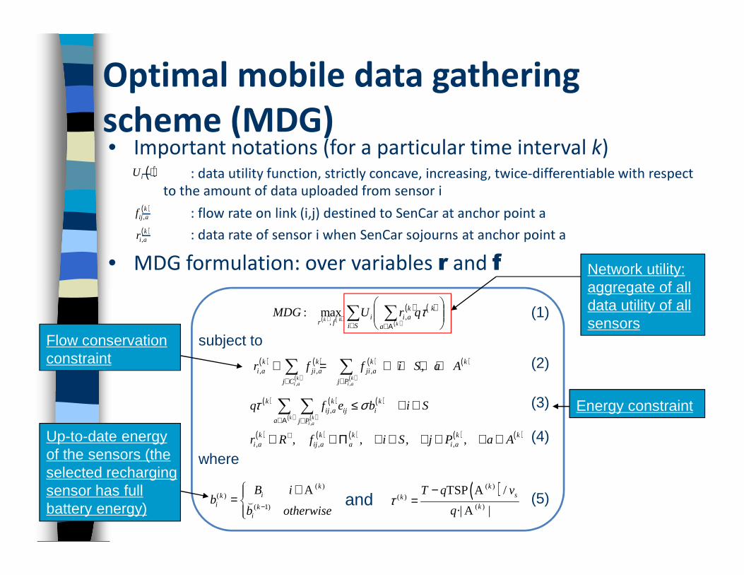
• Important notations (for a particular time interval k)– : data utility function, strictly concave, increasing, twice-differentiable with respect

to the amount of data uploaded from sensor i

– : flow rate on link (i,j) destined to SenCar at anchor point a

– : data rate of sensor i when SenCar sojourns at anchor point a

• MDG formulation: over variables r and f

Optimal mobile data gathering

scheme (MDG)

( ),k

ij af

( )iU ⋅

Network utility: aggregate of all

( ),k

i ar

aggregate of all data utility of all sensors

Energy constraint

Flow conservation constraint ( ) ( )

( )

( )

( )

( )

, ,

, , , ,k k

i a i a

k k k ki a ji a ji a

j C j P

r f f i S a A∈ ∈

+ = ∀ ∈ ∀ ∈∑ ∑

( ) ( )

( )

( )

( ),

,k k

i a

k k kij a ij i

a j P

q f e b i Sτ σ∈Α ∈

≤ ∀ ∈∑ ∑

( ) ( ) ( ) ( ) ( ), , ,, , , ,k k k k k

i a ij a a i ar R f i S j P a A+∈ ∈Π ∀ ∈ ∀ ∈ ∀ ∈

(

)

(

1

)

(

)

ki

kik

i

i

b otherwis

Bb

e−

∈= (

Aand ( )( )

( )( )

TSP /

·| |

ksk

k

T q v

qτ

−=

A

A

( ) ( )( ) ( )

( )∑ ∑∈ Α∈

Si a

kkaii

fr kkk

qrUMDG τ,,

max:

subject to

where

(1)

(2)

(3)

(4)

(5)

Up-to-date energyof the sensors (theselected rechargingsensor has fullbattery energy)

• MDG lacks of strict concavity

• Proximal approximation based algorithm

• Iterative steps in proximal approximation– Add a quadratic term

• x is an additional vector and c is a positive constant

– In iteration t

MDG: solution

( )( )

2( ) ( ) 2 ( ) ( )2 , ,

1 1

2 2 k

k k k ki a i a

i ar x

c c ∈ ∈− − = − −∑ ∑r x‖ ‖

S A

• Distributed implementation developed based on dual

decomposition

Step 1: Fix for all and and solve the

following problem to obtain the optimal and .

subject to constraints (2), (3) and (4).

Step 2: Set for all and .

( ) ( ), , [ ]k k

i a i ax x t= i ∈ S ( )ka ∈A( ), [ ]k

i ar t ( ), [ ]k

ij af t

( ) ( ) ( )

( ) ( ) ( ) ( ) 2, 2

,

1max

2k k k

k k k ki i a

i aU r q

cτ

∈ ∈

− −

∑ ∑r f

r x‖ ‖S A

(5)

( ) ( ), ,[ 1] [ ]k k

i a i ax t r t+ = i ∈ S ( )ka ∈A

MDG: solution (cont.)

( ) ( ) ( )

( ) ( ) ( ) ( ) 2, 2

,

1max

2k k k

k k k ki i a

i aU r q

cτ

∈ ∈

− −

∑ ∑r f

r x‖ ‖S A

subject to constraints (2), (3) and (4).

( ) ( ) ( ) ( )

( ) ( ) ( )

0 ,min ( ) min max ( , , )

k k k k

k k kg Lλ

λ =λ r f

r f λ±

� Solving problem

Dual decomposition

Under the Karush-Kuhn-Tucker (KKT)

conditions, it can be solved with

complexity .( ) ( )(| | log(| |))k kO A A

( ) ( ) ( ) ( ) 2 ( ) ( ), , , , ,

1( ) ( )

2k k k k k k

i i a i a i a i a i aa a a

U r q r x rc

τ λ− − −∑ ∑ ∑

Sub-Prob1: Rate Control

Scheduling: maximum

weighted matching

Routing: greedy

allocation

Sub-Prob2: Joint Scheduling and Routing

( ) ( ) ( ), , ,( )k k k

i a j a ij ai a j

fλ λ−∑∑∑

( ) ( ) ( ),· ,k k k

ij a ij ia j

q f e b iτ σ< ∀ ∈∑∑ S

( ) ( ) ( ) ( ), ,, , ,k k k k

ij a a i af i j a∈Π ∀ ∈ ∀ ∈ ∀ ∈S P A

s.t.

max

( ) ( ) ( ) ( ) ( ), , , , ,[ 1] [ ] [ ] [ ] [ ] [ ]k k k k k

i a i a i a ji a ij aj j

n n n r n f n f nλ λ θ+

+ = + + − ∑ ∑ Sub-gradient Projection

r fλ

� Network setup– 100m×100m area– 10 wireless rechargeable sensors– Utility function– 1 hour for each time interval length T

3. Numerical results

( ),( ) log( 1)k

i i i aa

U w r qτ⋅ = +∑– 1 hour for each time interval length T– 5 migration tours in each time interval.

� Parameter settings

Parameter Value Parameter Value

2100mAh 0.3mJ/Kbit

100 0.02J/Kbit

200m

1m/s 0.9

iB ije

iwiie Λ

( )nθ 1

1 10n+

sv σ

L

� Convergence of proximal approximation based algorithm� Data rates: stable after 10 iterations

� Recovered flow rates: differences within 5% of their optimal values

after 500 iterations

Convergence of Proximal

Approximation Based Algorithm

(a) Evolution of data rates versus

proximal iterations t.

(b) Evolution of recovered flow rates

versus subgradient iterations n.

� High network utility & perpetual network operations� Higher cumulative network utility can be obtained in the cases with a

smaller T.

� More chances for energy replenishment under a smaller T.

� 9 times (T = 1 hour) v.s. twice (T = 6 hours).

Performance of J-MERDG

(a) Cumulative network utility. (b) Battery states of sensor 8.

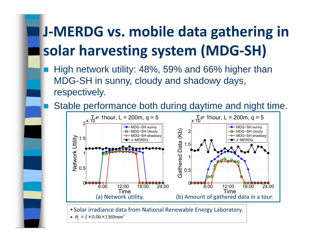
J-MERDG vs. mobile data gathering in

solar harvesting system (MDG-SH)� High network utility: 48%, 59% and 66% higher than

MDG-SH in sunny, cloudy and shadowy days, respectively.� Stable performance both during daytime and night time.

(a) Network utility. (b) Amount of gathered data in a tour.

• Solar irradiance data from National Renewable Energy Laboratory.

• 2136906.0 mmIr ××=π

4. Conclusion

� Joint design of energy replenishment and data gathering (J-MERDG) by exploiting mobility: the first work.

� Anchor points selection algorithm: balance between the energy replenishing range and data gathering latency.

� Flow-level network utility maximization model. We propose a proximal approximation based algorithm to obtain the system-wide proximal approximation based algorithm to obtain the system-wide optimum by adjusting data rates, link scheduling and flow routing in a distributed manner.

� Extensive numerical results: perpetual operations of the network AND significant network utility enhancement (outperforms solar harvesting system by 48%).

Thank you!Thank you!