joint scheduling of overlapping phases in the mapreduce ... filerelated work: strong pair minimize...
TRANSCRIPT

1
Joint Scheduling of Overlapping Phases in the MapReduce Framework
Jie Wu
Collaborators: Huanyang Zheng and Yang ChenCenter for Networked Computing
Temple University

2
Road Map
1. Introduction
2. Model and Formulation
3. General Greedy Solutions
4. Experiment
5. Conclusion

3
1. Introduction
Map-Shuffle-Reduce: a popular computation paradigmMap and Reduce: CPU-intensiveShuffle: I/O-intensive
Master node: pipeline schedulingData node: data parallelism
E.g., TeraSortMap: sample & partition dataShuffle: move dataReduce: locally sort data
Shuffle
Data partition
Map Reduce
Local sort
Data partition
Local sort

4
Scheduling of Multiple Jobs
Multiple jobsTerasort, wordcount, …
Reduce is not significant (Zaharia, OSDI 2008)7% of jobs are reduce-heavy
Centralized schedulerDetermines a sequential order for jobs on the map and shuffle pipeline

5
Job Classification
Dependency relationshipMap emits data at a certain rateShuffle waits for the map data
Job classificationMap-heavy: map ≥ shuffle (m ≥ s)Shuffle-heavy: map ≤ shuffle (m ≤ s)

6
Time
Time
0%
100%
0%
100%J2
J2J1
J1
Map CPU
Shuffle I/O
2 310
Time
Time
0%
100%
0%
100%J2
J2 J1
J1
Map CPU
Shuffle I/O
2 3 40
Execution Order
Impact of overlapping map and shuffle
Map pipeline
Shuffle pipeline
WordCount (map-heavy) TeraSort (shuffle-heavy)

7
2. Model and Formulation
Schedule objective:Minimize the average job completion time for all jobs; Ji includes the wait time before the job starts.
Schedule is NP-hard offline and APX-hard online (Lin 2013)
Offline All jobs arrive at the beginning (and wait for
schedule)

8
Related Work: Flow ShopMinimize last job completion time
l-phase flow shop is solvable when l=2○Gs: shuffle-heavy jobs sorted in decreasing order of shuffle load○Gm: map-heavy jobs sorted in increasing order of map load
Optimal schedule: Gs followed by Gm
S. M. Johnson, Optimal two-and three-stage production schedules with setup times included, Naval Research Logistics Quarterly, 1954.
Map
Shuffle J2J2
J1J1
J3J3
J4J4
J2J2
J1J1
J3J3
J4J4

9
Related Work: Strong PairMinimize average job completion time
Strong pair○J1 and J2 are a strong pair if m1 = s2 and s1 = m2
Optimal schedule: jobs are strong pairsPair jobs and rank pairs by total workloads
H. Zheng, Z. Wan, and J. Wu, Optimizing MapReduce framework through joint scheduling of overlapping phases, Proc. of IEEE ICCCN, 2016.
Map
Shuffle J1J1
J3J3 J4
J4J2
J2J1J1
J3J3J4
J4J2
J2

10
First Special CaseWhen all jobs are map-heavy, balanced, or shuffle-heavy
Optimal schedule O(n log n):Sort jobs ascendingly by dominant workload max{m, s}
Execute small jobs first
Map pipeline
Shuffle pipeline
Time
Time
J1
J1
J2
J2
J3
J3Time
Time
J1
J1
J2
J2
J3
J3
Finishing times J1, J2, J3: 1, 3, 6 vs. J3, J2, J1: 3, 5, 6
11
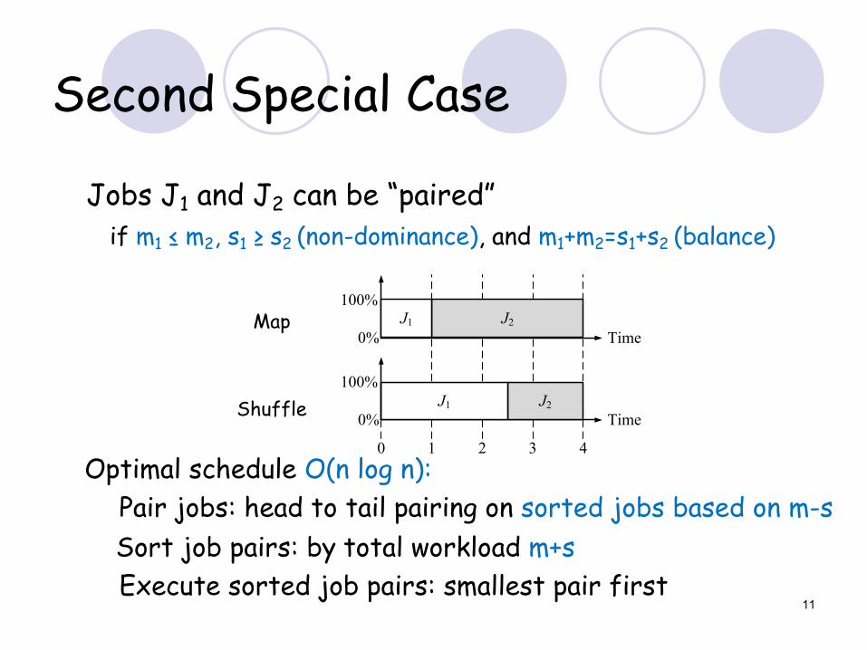
Second Special Case
Jobs J1 and J2 can be “paired”if m1 ≤ m2, s1 ≥ s2 (non-dominance), and m1+m2=s1+s2 (balance)
Optimal schedule O(n log n):Pair jobs: head to tail pairing on sorted jobs based on m-s Sort job pairs: by total workload m+sExecute sorted job pairs: smallest pair first
Map
Shuffle Time
Time
0%
100%
0%
100%J2
J2J1
J1
2 3 40 1

12
Why Non-dominance?Cannot pair small and large jobs J1 and J2
Time
Time
J1
J1
J2
J2
Map
Shuffle
0 1 2 3 4 5 6 7 8 9 10
Time
Time
J1
J1
J2
J2
Map
Shuffle
0 1 2 3 4 5 6 7 8 9 10
Completion times: 2, 5, and 10
Completion times: 3, 5, and 10

13
If jobs can be paired, paired job scheduling is optimal if(1) job pairs with smaller workloads are executed earlier and(2) all pairs are executed together (with shuffle-heavy first).
In each pair, shuffle-heavy job is executed before map-heavy jobOtherwise a swap leads to a better result
Job pairs with smaller total workloads are executed earlierOtherwise a swap leads to a better result
Paired jobs should not be separately executed A bit more involved
Theorem

14
S1 is better than S3 and S4 when J* is largeS2 is better than S3 and S4 when J* is small
Proof

15
3. General Greedy Solutions
A delicate balance for general cases
Map-dominant (shuffle-dominant)
more map (shuffle)-heavy than shuffle (map)-heavy
Pairingfactor
Small jobfactor

16
Sort jobs based on their sizes (“workload”)
Partition sorted list in k (group factor) groups
Execute each group in order based on workloadOrder matters for inter-group!
Pair jobs in each group Pairing matters for intra-group!
…...
Group
1 2 k -1
Working order
First Greedy Algorithm
17
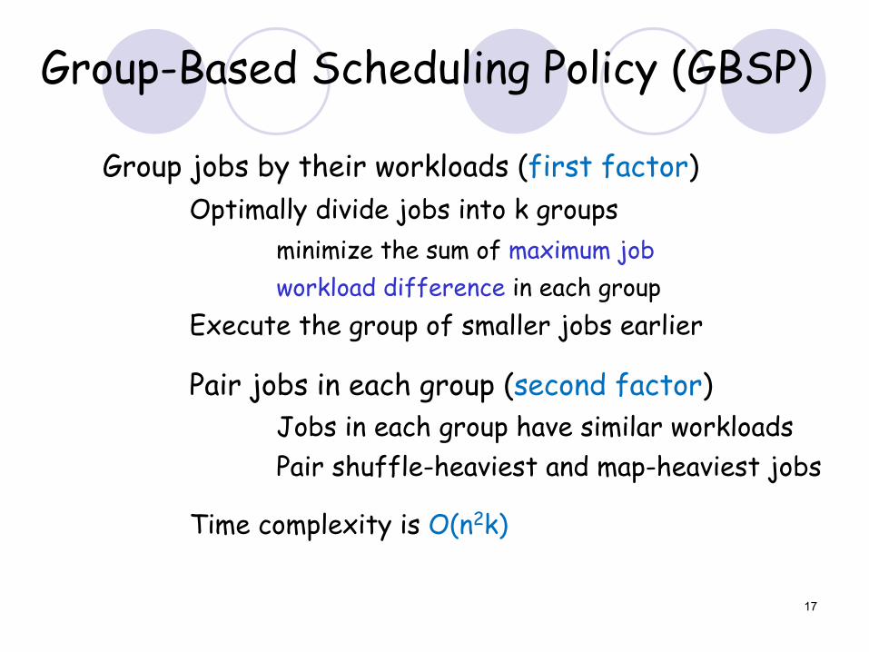
Group jobs by their workloads (first factor)Optimally divide jobs into k groups
minimize the sum of maximum jobworkload difference in each group
Execute the group of smaller jobs earlier
Pair jobs in each group (second factor)Jobs in each group have similar workloadsPair shuffle-heaviest and map-heaviest jobs
Time complexity is O(n2k)
Group-Based Scheduling Policy (GBSP)

18
Example 1: GBSP
J1
J1
J4
J4J2
J2 J3
J3
mapshuffle
group jobs by workloadsJ1
J1
J4
J4 J2
J2J3
J3
pair jobs in each groupJ1
J1
J4
J4 J2
J2 J3
J3
scheduleJ1
J1
J4
J4 J2
J2 J3
J3

19
Workload DefinitionDominant workload scheduling policy (DWSP)
Groups jobs by dominant workloads, max {m, s}Performs well when jobs are simultaneously map-heavy, balanced, or shuffle-heavy
Total workload scheduling policy (TWSP)Groups jobs by total workloads, m+s
Performs well when jobs can be perfectly paired
Weighted workload scheduling policy (WWSP)A tradeoff between DWSP and TWSP
Groups jobs by weighted workloads , α*max{m,s} + (1-α)*(m+s)

20
Second Greedy Algorithm Sort jobs by map-shuffle workload difference
Cut jobs into two partsUse minimum weight maximum matching to pair jobs in the first part
Exhaust all possible cuts and pick the best cutSort jobs by their workloads after pairing, together with single jobs
Paired jobs are regarded as one job
Sort jobs by m-s ( or )
Paired jobs Single jobsCut
Map-dominant
Paired jobs Single jobsCut
Shuffle-dominant
Sort jobs by s-m ( or )

21
Pair jobs through minimum weight maximum matchingMatching weight for J1 and J2:
(1-β) * non-dominance factor +β * balance factor
Non-dominance factor:Balance factor:
Match-Based Scheduling Policy (MBSP)
J5J5
J4J4J2
J2
J3J3
J1J1
J6J6
J7J7

22
TheoremMBSP has an approximation ratio of 2 if
(1) some jobs can be perfectly paired,(2) all remaining jobs are map-heavy or shuffle-heavy,(3) dominant workload is used to sort jobs.
Time complexity is O(n3.5)Exhausting all cuts takes O(n) iterationsMatching in each iteration takes O(n2.5)
(Blossom algorithm, 1961)

23
4. Experiment
Google Cluster SimulationAbout 11,000 machines96,182 jobs over 29 days in May 2011
Number of job submissions per hour (arrival rate)

24
Google Cluster Dataset
Distribution of map and shuffle time
Slightly more map-heavy jobs

25
Comparison Algorithms
Pairwise: has only one group then iteratively pairs themap-heaviest and shuffle-heaviest jobs in the group
MaxTotal: ranks jobs by total workload m+s and executes jobs with smaller total workloads earlier
MaxSRPT: ranks jobs by dominant workload max{m,s} and executes jobs with smaller dominant workloads earlier

26
Waiting, Execution, and CompletionGroup k = 20, α = 0.5, β = 0.5, Col 1st regular, 2nd shuffle half, 3rd map half
GBSP
The average job completion time ratio between MBSPand WWSP is 92.3%, 95.8% and 85.1%, respectively.
Scheduling algorithms Average jobwaiting time
Average jobexecution time
Average jobcompletion time
Pairwise 8289 7652 3609 149 23 28 8438 7675 3637
MaxTotal 5054 4586 2525 362 32 156 5416 4618 2681
MaxSRPT 4768 4546 2591 840 32 150 5608 4578 2741
DWSP 4809 4519 2545 581 53 85 5390 4572 2630
TWSP 4787 4501 2522 563 49 104 5350 4550 2626
WWSP 4619 4482 2479 532 45 79 5151 4527 2558
MBSP 4562 4314 2142 193 26 36 4754 4340 2178

27
Impact of k and α in WWSP
Group-based scheduling policy with k groupsSorts jobs by α*max(m,s) + (1-α)*(m+s)
Small/large group kSmall/large weight α
Minimized when α = 0.57

28
Impact of β in MBSP
Match-based scheduling policy matches J1 and J2 byβ * balance factor + (1-β) * non-dominance factor
Small/large weight βMinimized
when β = 0.68

29
Hadoop Testbed on Amazon EC2
TestbedUbuntu Server 14.04 LTS (HVM)Single core CPU and 8G SSD memory
Jobs: WordCount jobs and TeraSort jobs6 WordCount use books of different sizes
2MB, 4MB, 6MB, 8MB, 10MB, 12MB
6 TeraSort use instances of different sizes1KB, 10KB, 100KB, 1MB, 10MB, 100MB

30
Completion Time
Hadoop: one master node + several data nodesNumber of data nodes: 1, 2, 4, 8, 16
MBSP and WWSP have the best results

31
5. Conclusion
Map and Shuffle phases can overlapCPU and I/O resource
Objective: minimize average job completion time
Group-based and match-based schedulesOptimality under certain scenariosPairing factorSmall jobs factor

32
Shuffle
Map
Reduce
Time
Time
0%
100%
0%
100%J2
J2J1
J1
Time0%
100%J2J1
2 310
Future Work3-phase example
More simulationsImbalanced map and shuffleimpact of k, α, and β
Multiple phasesBeyond 2-phase
Other computation paradigmsMap-collective

33
Future WorkOnline scheduling
BatchedBatch size
Duration-based batchingLow-job rate: time out
High-job rate: probabilistic ∆: efficient, but slow; 1-∆: inefficient, but fast
Counting-based batchingLow-job rate: time out
High-job rate: creditScheduling time vs. execution time