joint shelf design and shelf space allocation problem for

Wright State University Wright State University

CORE Scholar CORE Scholar

Browse all Theses and Dissertations Theses and Dissertations

2020

Joint Shelf Design and Shelf Space Allocation Problem for Joint Shelf Design and Shelf Space Allocation Problem for

Retailers Retailers

Hakan Gecili Wright State University

Follow this and additional works at: https://corescholar.libraries.wright.edu/etd_all

Part of the Engineering Commons

Repository Citation Repository Citation Gecili, Hakan, "Joint Shelf Design and Shelf Space Allocation Problem for Retailers" (2020). Browse all Theses and Dissertations. 2339. https://corescholar.libraries.wright.edu/etd_all/2339

This Dissertation is brought to you for free and open access by the Theses and Dissertations at CORE Scholar. It has been accepted for inclusion in Browse all Theses and Dissertations by an authorized administrator of CORE Scholar. For more information, please contact [email protected].

https://corescholar.libraries.wright.edu/

https://corescholar.libraries.wright.edu/etd_all

https://corescholar.libraries.wright.edu/etd_comm

https://corescholar.libraries.wright.edu/etd_all?utm_source=corescholar.libraries.wright.edu%2Fetd_all%2F2339&utm_medium=PDF&utm_campaign=PDFCoverPages

http://network.bepress.com/hgg/discipline/217?utm_source=corescholar.libraries.wright.edu%2Fetd_all%2F2339&utm_medium=PDF&utm_campaign=PDFCoverPages

https://corescholar.libraries.wright.edu/etd_all/2339?utm_source=corescholar.libraries.wright.edu%2Fetd_all%2F2339&utm_medium=PDF&utm_campaign=PDFCoverPages

mailto:[email protected]

JOINT SHELF DESIGN AND SHELF SPACE ALLOCATION PROBLEM

FOR RETAILERS

A dissertation submitted in partial fulfillment of the

requirements for the degree of

Doctor of Philosophy

By

HAKAN GECILI

B.S., Turkish Naval Academy, Turkey, 2002

M.S., Kocaeli University, Turkey, 2012

2020

Wright State University

WRIGHT STATE UNIVERSITY

GRADUATE SCHOOL

Jun 24, 2020

I HEREBY RECOMMEND THAT THE DISSERTATION PREPARED UNDER MY

SUPERVISION BY Hakan Gecili ENTITLED Joint Shelf Design and Shelf Space

Allocation Problem for Retailers BE ACCEPTED IN PARTIAL FULFILLMENT OF THE

REQUIREMENTS FOR THE DEGREE OF Doctor of Philosophy.

________________________________

Pratik Parikh, Ph.D.

Dissertation Director

________________________________

Brian Rigling, Ph.D

Interim Director, Engineering PhD Program,

Professor and Dean, College of Engineering

and Computer Science

________________________________

Barry Milligan, Ph.D.

Interim Dean of the Graduate School

Committee on Final Examination:

_______________________________

Pratik Parikh, Ph.D.

________________________________

Xinhui Zhang, Ph.D.

________________________________

Subhashini Ganapathy, Ph.D.

________________________________

Nan Kong, Ph.D.

________________________________

Amir Zadeh, Ph.D.

iii

ABSTRACT

Gecili, Hakan Ph.D., Engineering Ph.D. program, Wright State University, 2020. Joint

Shelf Design and Shelf Space Allocation Problem.

Although the retail business has been exploring innovative ways to engage shoppers, the

COVID-19 pandemic has sped up their effort. Because of its unique benefits, physical stores will

continue to remain an integral part of the overall retail business. However, to stay competitive,

retailers will be forced to effectively utilize their available space in physical store (and even reduce

it if need be), while offering a reasonably large assortment of products on their shelves. For many

such retailers, the design of planograms – visual representation of products on shelves – is still

driven by prior experience and intuition. Further, existing optimization-based planogram design

approaches assume that the shelf length and height are fixed, which often result in unused space on

the planogram or suboptimal assignment of SKU facings, both resulting in reduced revenue for the

retailer.

To address this real-world challenge, we introduce the joint shelf design and shelf space

allocation (JSD-SSA) problem to maximize retailer’s revenue. Our proposed mathematical

programming model for JSD-SSA determines the optimal shelf design, while determining SKU

placement and facings, under SKU family constraints. Because realistic problem sizes pose

significant computational challenges in solving this model, we propose a decomposition-based

approach. Accordingly, we first partition the planogram area and allocate it to each SKU family

via a Particle Swarm Optimization heuristic, then for each partition we determine the shelf design

(number of shelves, shelf coordinates, length, and height) and shelf space allocation (SKU

iv

placement and facings) using Constraint Programming. In so doing, real-world problem instances

(2 families, 100 SKUs total, 192” × 84” planogram size) could be solved within 45 minutes. We

also propose a metric to measure variation in SKU shapes within and between SKU families.

Our experiments indicate that shorter shelf lengths can increase retailer’s profit by up to

22% depending on the SKU-family shape variation. Higher within-family shape variation can result

in higher revenue increases. Further, as the planogram becomes tighter (measured via space

tightness), the benefits of shorter shelf lengths increase. Additionally, if SKU and planogram

dimensions share a common factor or multiple, then more compact planograms can be designed, in

turn reducing unused space and increasing retailer’s profit.

We strongly believe that our optimization-based approach will allow retailers to fully

utilize the available shelf space, especially during post COVID-19 environment where retailers may

opt to reduce their store footprint. Better SKU allocation on highly visible shelf locations will allow

better shopper-SKU interaction, in turn reduce expensive trial-and-errors. Our approach will also

allow benchmarking of existing and alternative planogram designs depending on the location of

the department in the store and corresponding shopper traffic.

v

TABLE OF CONTENTS

1. INTRODUCTION ....................................................................................................................... 1

2. LITERATURE REVIEW ............................................................................................................ 5

2.1. Shelf space allocation ........................................................................................................... 5

2.2. Planogram layout .................................................................................................................. 6

3. A MODEL FOR THE JSD-SSA PROBLEM .............................................................................. 9

4. A HYBRID DECOMPOSITION-BASED APPROACH FOR JSD-SSA PROBLEM ............. 14

4.1. Subproblem (i): PSO-based planogram partitioning ........................................................... 15

4.1.1. Guillotine cut algorithm and PSO solution representation .......................................... 15

4.1.2. Necessary conditions for feasibility and calculation of penalty ................................... 17

4.2. Subproblem (ii): CP-based solution for the reduced problem ............................................ 17

4.3. Performance of the proposed approach ............................................................................... 18

5. EXPERIMENTAL STUDY ....................................................................................................... 21

5.1. Data generation and data collection .................................................................................... 21

5.2. SKU shape variation ........................................................................................................... 21

5.2. Space fitness ....................................................................................................................... 24

6. CASE STUDY ........................................................................................................................... 31

7. CONCLUSION AND FUTURE RESEARCH .......................................................................... 33

REFERENCES .............................................................................................................................. 35

APPENDICES ............................................................................................................................... 41

Appendix A. Comparison of CPLEX and CP performances for subproblem (ii) ...................... 41

Appendix B. PSO-CP Convergence Table ................................................................................ 43

Appendix C. Experiment Results ............................................................................................... 44

vi

Appendix D. Case Study Results ............................................................................................... 45

vii

LIST OF FIGURES

Figure 1. Gondola shelves with mixed length and height ................................................................ 2

Figure 2. The schematic of the hybrid decomposition-based PSO-CP approach .......................... 15

Figure 3. A solution representation and partitioning for a 3-family planogram ............................ 16

Figure 4. MAL and MAA .............................................................................................................. 21

Figure 5. The joint distribution of MAA and MAL ....................................................................... 22

Figure 6. Homogeneity/Heterogeneity of clusters ......................................................................... 23

Figure 7. 2D k-means clustering of TW and TWiB ....................................................................... 24

Figure 8. Change in RIR with respect to SF and shape variation across various shelf lengths ..... 26

Figure 9. SKU arrangement in 60”-shelf and customized shelf designs for SF=0.28 and SF=0.16

....................................................................................................................................................... 28

Figure 10. Factors and multiples .................................................................................................... 30

Figure 11. Shelf design and SKU position for the two planograms............................................... 31

viii

LIST OF TABLES

Table 1. Shelf space allocation models ............................................................................................ 7

Table 2. Sets and parameters ......................................................................................................... 10

Table 3. Decision variables ............................................................................................................ 10

Table 4. The performance of PSO-CP algorithm ........................................................................... 19

Table 5. Experiment design factors and levels .............................................................................. 25

Table 6. RIR across various experimental settings ........................................................................ 25

Table 7. Average RIR over 60”-shelf length ................................................................................. 26

ix

ACKNOWLEDGEMENTS

I would like to offer my special thanks to Dr. Pratik Parikh for his continuous support and guidance

during the development and delivery of this research. Dedication of his time and personal support

has been greatly appreciated.

Thank you Dr. Xinhui Zhang for your constant help and supervision for many years, which

changed my life and facilitated this research. I also appreciate the valuable suggestions and

comments of my committee.

To Melanie Gecili, thank you for your support and friendship through the transition of my life

and education.

To my son Deniz Kaan Gecili and my parents Veli and Kevser Gecili, thank you for all the

love and support.

Finally, I want to thank all my friends and family for encouraging me to pursue my degree.

1

1. INTRODUCTION

The proliferation of new products and product variants, changes in customers’

expectations, finite and scarce retail shelf space, and thin profit margins make the retail industry

very competitive (Curhan, 1972; Zufryden, 1986; Lim et al., 2004; J. M. Hansen et al., 2010). To

meet the dynamic demand under limited space, retail managers frequently attune their assortments

and planograms (J Irion et al., 2011); improved space utilization via effective space management

approaches have become even more critical to stay competitive (Geismar et al., 2015).

A common problem in this area is the Shelf Space Allocation (SSA); i.e., the decision of

which products are selected and how many faces are shown. The goal of SSA is to increase sales

of a product by increasing its perceptibility (P. Hansen & Heinsbroek, 1979), reduce stock-outs,

and decrease managerial expenses such as labor cost (Lim et al., 2004) by accounting for computer-

aided shelf space management approaches to enhance customer satisfaction have, therefore,

become popular (Yang, 2001).

Although a variety of approaches have been presented to address the SSA, some of which

account for demand characteristic (substitution, space, and cross-space elasticity), varying features

of products (types, dimensions, prices, families), and other merchandising constraints, they all

either ignore shelves or assume that the shelf dimensions are prespecified. Researchers, ignoring

the shelf structure, use only one dimension of products (area, space or length) and assume that

products have a liquid form. However, most product packagings are reasonably rigid and have

specific geometry. Studies that acknowledge that products have a unique shape (slot allocation) or

they can fit on shelves no matter what the allocation is, assume a fixed shelf design. However, a

mismatch between product geometry and the shelf opening can create unused space between the

2

top of products and the shelves above them. While shelf space allocation is also jointly considered

with assortment planning in many studies (Borin et al., 1994; Smith & Agrawal, 2000; Kök &

Fisher, 2007; J Irion et al., 2011; Jens Irion et al., 2012), the deficiencies mentioned here are even

more pronounced in those setups. Because new product dimensions in an adjusted assortment can

make the layout infeasible, therefore a new assortment can dictate a new shelf design.

Interestingly, our observations at stores of nearby retailers suggest that stores commonly

use different sized bays for gondola and peg shelves. These types of racks can accommodate shelves

with different height and lengths. As for 2020, most commonly used shelf lengths are 24 in., 36 in.,

48 in. and heights are 54 in., 60 in., 72 in. and 84 in. Besides, products come with many shapes and

sizes, and retailers use mixed shelf lengths and heights in an attempt to efficiently utilize the

planogram area (Figure 1).

Figure 1. Gondola shelves with mixed length and height

The lack of scientific approaches to determine the best configuration of their shelves and

allocate products to it, in turn, results in retailers resorting to expensive trial-and-errors. This begs

the question: What would the ideal mix of shelf lengths and heights on a rack that achieves this

goal? How much more would the expected revenue increases be? Would such configurations be

optimal in all settings? What factors affect the design of such shelves?

To the best of our knowledge, the joint problem of shelf design and shelf space allocation

has yet to be studied. In this paper, we propose an optimization-based approach for, what we now

3

refer to as, the Joint Shelf Design and Shelf Space Allocation (JSD-SSA) problem. In so doing, we

make the following contributions:

1. We propose a Mixed Integer Programming (MIP) model for JSD-SSA, which determines the

number of shelves, their height, length, and position on a 2D planogram, along with the

standard SSA decisions by taking the adjacency and alignment constraints of product families

into consideration. The objective of JSD-SSA is to maximize retailers’ daily revenue per

planogram.

2. While small instances of this problem can be solved efficiently using a commercial solver,

realistic problem sizes (e.g., 100 products, planogram height 72” and length 120”) pose

significant computational challenges. Our proposed hybrid approach decomposes the problem

into two subproblems: (i) SKU family-to-location and (ii) shelf-sizing and product placement.

This approach effectively uses the Particle Swarm Optimization (PSO) to solve subproblem (i)

and, for each particle, uses Constraint Programming (CP) to solve subproblem (ii). We compare

the performance of our proposed approach to CPLEX and CP-only approaches on small

instances to demonstrate its viability.

3. We evaluate the sensitivity of the derived solutions to varying levels of heterogeneity in SKU

sizes and planogram sizes. Our experiments are based on real data, which is derived from more

than 35,000 planograms available from a leading US retailer. In so doing, we generate

managerial insights of immediate use for the retailers.

Based on our experiment designs, we observe that as the homogeneity increases, the model

tends to create longer shelves, and as the heterogeneity increases the model creates mixed shelf

length and heights. Our experiment results showed that as planogram space gets tighter, shorter

shelves become more beneficial. We also observed that if SKU shapes are heterogeneous, the

proposed shelf design model can increase the profit by 22%. Finally, we found that the allocation

4

of SKUs sharing a common factor or multiples in SKU dimensions, and the planogram dimensions

tend to utilize the planogram space better.

The rest of the article is structured as follows: Section 2 outlines the literature review of Shelf

Space Allocation. Section 3 builds the mathematical model for shelf design and SKU allocation,

and Section 4 describes the decomposition-based solution approach. Section 5 describes the retail

data, experimental study, and presents key insights for retailers. Section 6 represents a case study.

Finally, we summarize the key findings and propose future studies in Section 7.

5

2. LITERATURE REVIEW

Shelf space allocation problem has been studied at three levels; store-wide, category-level,

and shelf-level (A. H. Hübner & Kuhn, 2012). Store and category planning studies consider

exposure to customer traffic as visibility and use the customer traffic distribution to optimize their

design (Chen & Lin, 2007; Flamand et al., 2016, 2018; Guthrie & Parikh, 2020).

Considering the focus of our work, below we now summarize the literature in the areas of

shelf-level space planning, that focus on determining the number of faces and locations of each

SKU.

2.1. Shelf space allocation

Shelf space allocation studies date back to the 1970s and are often modeled as Bounded

Knapsack Problem (BKP) or Multi Knapsack Problem (MKP). A Knapsack Problem (KP) is called

BKP, if the decision-maker determines the number of items to carry and it is called MKP if there

is more than one knapsack (Martello & Toth, 1990). From the KP point of view, SSA models are

considered as BKP, where retailer decides the number of faces of each SKU. Some SSA models

divide the planogram area into multiple shelves (with prespecified dimensions) and solve the SSA

problem as an MKP (Yang, 2001).

In most SSA models demand is modeled by using elasticity (space/price) and inventory

terms. In the retail industry, space elasticity is defined as an increase/decrease in demand in

response to changes in the space of a product. Shelf space elasticity has been considered in several

SSA studies ( Brown & Tucker, 1961; Corstjens & Doyle, 1981; J. M. Hansen et al., 2010; Jens

Irion et al., 2012; A. Hübner & Schaal, 2017; Bianchi-Aguiar et al., 2018) and assortment planning

6

models (P. Hansen & Heinsbroek, 1979). However, some later studies preferred simplicity and

linearized their models by excluded the elasticity terms ( Yang & Chen, 1999; Yang, 2001).

Many SSA studies further include inventory decisions into their models, as SSA is closely

associated with inventory. Various aspects of inventory were incorporated into SSA. Corstjens &

Doyle (1983) studied the inventory of products with increasing demand trends, Bai & Kendall

(2008) modeled the effect of the freshness of inventory in SSA, Urban (2002) and Hariga et al.

(2007) examined the impact of declining shelf inventory on SSA. More complicated models

incorporated inventory decisions with SSA and assortment planning (Urban, 1998, 2002). For a

detailed literature review on SSA, we refer to Hübner & Schaal (2017). However, these prior works

do not consider the positions of SKUs. Consequently, shelf design is not a part of their models

2.2. Planogram layout

Planogram layout optimization models calculate the number of faces considering

positioning and merchandising rules. Positioning rules typically include non-overlapping SKU

allocation, shelf dimensions, stocking and orientation of SKUs, and horizontal/vertical location

effects.

Merchandising rules dictate some clustering and replenishment constraints on layout

optimization. Customers expect to see similar products together; brands can buy positions on

shelves to compete better. Available labor can dictate the number of faces on shelves due to limited

replenishment frequency and amount. Hwang et al. (2009) considered the rectangular area and

adjacency constraints by partitioning the planogram area for SKUs using guillotine cuts. They

created a model similar to facility design models and solved it through a genetic algorithm. Russell

& Urban (2010) presented a mixed-integer quadratic layout optimization model, which takes the

product adjacency and vertical and horizontal location effects into consideration. Geismar et al.

(2015) allocated products in a rectangular area in their unit length shelf-space allocation model for

a DVD store. Bianchi-Aguiar et al. (2018) proposed a mixed-integer model to allocate families of

SKUs in rectangular clusters by considering their family hierarchy. A recent study by A. Hübner

7

et al. (2020) partitioned the shelf area into rectangles and assigned facings in 3D (X-Y-Z). They

solved the layout and assortment planning problem jointly by using a genetic algorithm.

Horizontal/vertical location effects on demand have been discussed by many authors, with

some conflicting evidence. Models considering these effects assume that SKUs at eye level are

more visible and have higher impulse purchase rates. Frank &Massy (1970) used multiple

regression analysis to estimate location effects and concluded that height does not have a significant

impact on sales. However, Drèze et al. (1994) suggested that horizontal location does not have a

notable effect on sales, however, the vertical location does. The horizontal location effect was also

examined by van Nierop et al. (2008) where they evaluated the interaction between the shelf layout

and marketing activities. They concluded that horizontal location/promotion effects are weak for

products that are not close to a racetrack. Yet, J. M. Hansen et al. (2010) argued that the number of

facings and vertical/horizontal positions have a significant effect on items’ profitability.

Some other positioning considerations in layout optimization are stackable and rotatable

products and inventory. Stacking and orientation variables enable better utilization of the shelf area,

and they were studied by Murray et al. (2010) and Bai et al. (2013). The layout and inventory were

studied jointly by Hwang et al. (2005), in which they proposed a model to determine how much of

an item to order, how many facings to allocate, and where to allocate them. They solved their model

using a gradient search heuristic and a genetic algorithm.

Table 1. Shelf space allocation models

Model Authors

No positioning P. Hansen & Heinsbroek, 1979; Corstjens & Doyle, 1981, 1983; Zufryden,

1986; Bultez & Naert, 1988; Borin et al., 1994; Urban, 1998, 2002; Yang &

Chen, 1999; Yang, 2001; Lim et al., 2004; Bai & Kendall, 2005, 2008;

Hariga et al., 2007; Gajjar & Adil, 2011; A. Hübner & Schaal, 2017

Fixed shelf

length and height

van Nierop et al., 2008; J. M. Hansen et al., 2010; Murray et al., 2010;

Russell & Urban, 2010; Bai et al., 2013; Geismar et al., 2015; Bianchi-

Aguiar et al., 2018

Planogram area

partitioning

Hwang et al., 2009; A. Hübner et al., 2020

8

Our review of the extant literature indicates that previous studies either ignore the existence

of shelf structure or they assume that shelves are fixed or given (Table 1). However, retail shelf

bays have slots (see Figure 1) to enable retailers to adopt varying shelf positions according to

product types. We do not know of any model in the academic literature that would allow retailers

to jointly optimize the shelf design and SSA decisions to maximize their revenue. Through this

research, we address this gap in the SSA literature and detail our approach below.

9

3. A MODEL FOR THE JSD-SSA PROBLEM

The JSD-SSA in this paper is defined as follows; given a planogram space and assortment which

shelf design and SKU allocation can yield the maximum profit? Shelf design is controlled by the

number of shelves, their dimensions (length, height), and coordinates (vertical, horizontal). SKU

allocation is done by determining the number of faces and their coordinates in a 2D plane.

We make the following assumptions in developing our model:

• The assortment and dimensions of SKUs, and the planogram area are known; upper bounds

and family clusters for each SKU are given.

• All SKUs must be allocated; product orientation and stacking decisions are known a priori.

• The visual location effect in both horizontal and vertical directions is uniform.

• Products are assumed to have a rectangular shape; if the product shape is not rectangular,

then the minimum-encapsulating rectangle (bounding-box) is assumed to be the shape of

that product.

Further, depending on the size of the store, retailers allocate one planogram for each type

of commodity. Within a commodity type, SKUs can be clustered in multiple hierarchies, based on

their types, brands, size, taste, etc. To reduce customer search effort, retailers commonly allocate

each hierarchy level of SKUs in a rectangular area, and all SKUs in one level should respect the

boundaries defined by the upper-level hierarchy. For example, in a planogram designated for pet-

food, customers do not expect to see food for cats and birds mixed up on the same shelf. This study

assumes two-level hierarchy; sub-commodity (e.g., cat and bird) and SKU. Rectangular area

allocation requires facings of SKUs and SKUs of sub-commodities to be adjacent in the horizontal

or vertical direction.

10

Parameters and decision variables used in the JSD-SSA model are summarized in Tables

2 and 3.

Table 2. Sets and parameters

Notation Definition

I ≡ {1,2,3, …, N} Set of SKU; i, j I

F ≡ {1,2,3, …, R} Set of family; f, g F

K ≡ {1,2,3, …, m} Set of shelves; k, p K

PW, PH Planogram length/height (in inches)

Pi Price of SKU i (in $)

Li, Di Minimum, maximum number of facing for SKU i

Wi, Hi Length/height of SKU i (in inches)

Zi, Ei Maximum face length/height allocation for SKU i

Tif 1 if SKU i is a member of family f; 0, otherwise

S-, S+ Minimum and maximum number of shelves

H-, H+ Minimum and maximum shelf height

W-, W+ Minimum and maximum shelf length

VS, VF Tolerance length for SKU and family alignment

Table 3. Decision variables

Notation Definition

m Number of shelves

sxk, syk x/y coordinate of the left/bottom corner of shelf k

shk, swk Height/length of shelf k (in inches)

txkp, t

ykp 1, if shelf k is strictly to the east/north of shelf p; 0, otherwise

xik, yik x/y coordinate of the left/bottom corner of the SKU i on shelf k

zij 1, if SKU i is strictly to the east of SKU j; 0, otherwise

sik 1, if SKU i is allocated on shelf k; 0, otherwise.

wik Number of faces of SKU i on shelf k

ui, bi Top/bottom shelf of SKU i

vfk 1, if family f is allocated on shelf k; 0, otherwise

lfk, rfk Left/right coordinate of family f on shelf k

fuf, fbf Top/bottom shelf of family f

The objective function is to maximize the total revenue across all SKUs for the retailer.

This objective function is similar to Yang & Chen (1999), where we use a linear model whereby

the visual location effect in the vertical direction is uniform and that the upper bound for demand

can be approximated by using historical point of sales data (which defines the maximum number

of facings for each SKU).

11

Maximize ∑ ∑ 𝑃𝑖𝑤𝑖𝑘𝑘𝑖 (1)

Subject to

Shelf design constraints 𝑠𝑥𝑘 + 𝑠𝑤𝑘 ≤ 𝑃𝑊 ∀𝑘 (2)

𝑠𝑦𝑘 + 𝑠ℎ𝑘 ≤ 𝑃𝐻 ∀𝑘 (3)

𝑠𝑥𝑘 + 𝑠𝑤𝑘 ≤ 𝑠𝑥𝑝 + 𝑃𝑊(1 − 𝑡𝑘,𝑝𝑥 ) ∀(𝑘, 𝑝), 𝑘 ≠ 𝑝 (4)

𝑠𝑦𝑘 + 𝑠ℎ𝑘 ≤ 𝑠𝑦𝑝 + 𝑃𝐻(1 − 𝑡𝑘,𝑝𝑦

) ∀(𝑘, 𝑝), 𝑘 ≠ 𝑝 (5)

𝑡𝑘,𝑝𝑥 + 𝑡𝑝,𝑘

𝑥 + 𝑡𝑘,𝑝𝑦

+ 𝑡𝑝,𝑘𝑦

≥ 1 ∀(𝑘, 𝑝), 𝑘 < 𝑝 (6)

Shelf design constraints (2)-(6) are similar to facility layout design constraints used in

Montreuil (1991) and Heragu & Kusiak (1991). Specifically, constraints (2-3) ensure that all

shelves are allocated within the planogram area, while constraints (4-6) ensure that shelf areas do

not overlap.

SKU allocation constraints

𝐿𝑖 ≤ ∑ 𝑤𝑖𝑘𝑘 ≤ 𝐷𝑖 ∀𝑖 (7)

𝑤𝑖𝑘 = 0 ∀𝑖, ∀𝑘 ∶ 𝐻𝑖 > 𝑠ℎ𝑘 (8) ∑ (𝑤𝑖𝑘 𝑊𝑖)𝑖 ≤ 𝑠𝑤𝑘 ∀𝑘 (9)

𝑤𝑖𝑘𝑊𝑖 ≤ 𝑍𝑖 ∀𝑖, ∀𝑘 (10)

𝑤𝑖𝑘 − 𝑀𝑠𝑖𝑘 ≤ 0 ∀𝑖, ∀𝑘 (11)

𝑤𝑖𝑘 − 𝑠𝑖𝑘 ≥ 0 ∀𝑖, ∀𝑘 (12)

∑ 𝑠𝑖𝑘𝑖 ≥ 1 ∀𝑘 (13)

𝑥𝑖𝑘 ≥ 𝑠𝑖𝑘𝑠𝑥𝑘 ∀𝑖, ∀𝑘 (14)

𝑥𝑖𝑘 + 𝑤𝑖𝑘𝑊𝑖 ≤ 𝑠𝑥𝑘 + 𝑠𝑤𝑘 ∀𝑖 , ∀𝑘 (15)

𝑦𝑖𝑘 = 𝑠𝑖𝑘 𝑠𝑦𝑘 ∀𝑖 , ∀𝑘 (16)

𝑥𝑖𝑘 + 𝑤𝑖𝑘𝑊𝑖 ≤ 𝑥𝑗𝑘 + 𝑠𝑤𝑘 (1 − 𝑧𝑖𝑗) ∀𝑘 , ∀(𝑖, 𝑗), 𝑖 ≠ 𝑗 ∶ 𝑠𝑖𝑘 + 𝑠𝑗𝑘 > 1 (17)

𝑧𝑖𝑗 + 𝑧𝑗𝑖 = 1 ∀(𝑖, 𝑗), 𝑖 ≠ 𝑗 ∶ 𝑠𝑖𝑘 + 𝑠𝑗𝑘 > 1 (18)

𝑥𝑖𝑘 − 𝑥𝑖𝑝 ≤ 𝑉𝑆 ∀(𝑘, 𝑝), 𝑘 ≠ 𝑝 , ∀𝑖 ∶ 𝑠𝑖𝑘 + 𝑠𝑖𝑝 > 1 (19)

𝑥𝑖𝑝 − 𝑥𝑖𝑘 ≤ 𝑉𝑆 ∀(𝑘, 𝑝), 𝑘 ≠ 𝑝 , ∀𝑖 ∶ 𝑠𝑖𝑘 + 𝑠𝑖𝑝 > 1 (20)

𝑤𝑖𝑘 − 𝑤𝑖𝑝 ≤ 1 ∀(𝑘, 𝑝), 𝑘 ≠ 𝑝 , ∀𝑖 ∶ 𝑠𝑖𝑘 + 𝑠𝑖𝑝 > 1 (21)

𝑤𝑖𝑝 − 𝑤𝑖𝑘 ≤ 1 ∀(𝑘, 𝑝), 𝑘 ≠ 𝑝 , ∀𝑖 ∶ 𝑠𝑖𝑘 + 𝑠𝑖𝑝 > 1 (22)

𝑠𝑖𝑘 = 1

∀𝑖 , ∀𝑘 ∶ 𝑏𝑖 ≤ 𝑠𝑦𝑘 ≤ 𝑡𝑖 ∧ ~ (𝑠𝑥𝑘 + 𝑠𝑤𝑘 < 𝑥𝑖𝑘 ∧ 𝑥𝑖𝑘 + 𝑤𝑖𝑘𝑊𝑖

< 𝑠𝑥𝑘 )

(23)

𝑏𝑖 ≤ 𝑃𝐻 − (𝑃𝐻 − 𝑦𝑖𝑘𝑠𝑖𝑘) ∀𝑖, ∀𝑘 (24)

𝑢𝑖 = 𝑚𝑎𝑥{𝑠𝑖𝑘𝑠𝑦𝑘: 𝑘 ∈ 𝐾} ∀𝑖 (25)

𝑢𝑖 ≥ 𝑏𝑖 ∀𝑖 (26)

𝑢𝑖 − 𝑏𝑖 ≤ E𝑖 ∀𝑖 (27)

12

Constraints (7) define bounds for the total number of facings for each SKU. Constraints

(8) and (9) ensure that an SKU’s height/total length complies with its shelf height/length. We

control the maximum horizontal/vertical SKU allocation length by using constraints (10) and (27).

Constraints (11) and (12) state that an SKU can have facings only on its allocated shelves.

Constraints (13) guarantee that all SKUs are allocated. Constraints (14) and (15) determine

coordinates of SKUs. Constraints (17) and (18) ensure that SKU areas do not overlap. If facings of

an SKU spread over multiple shelves constraints (19) – (22) ensure left and right alignment with a

given tolerance. Constraints (23) guarantee vertical adjacency for SKU faces. Constraints (24) -

(26) define top/bottom shelf coordinates.

Family constraints

∑ ( 𝑇𝑖𝑓𝑠𝑖𝑘)𝑖 − 𝑀𝑣𝑓𝑘 ≤ 0 ∀𝑓, ∀𝑘 (28)

∑ ( 𝑇𝑖𝑓𝑠𝑖𝑘)𝑖 − 𝑣𝑓𝑘 ≥ 0 ∀𝑓, ∀𝑘 (29)

𝑙𝑓𝑘 ≤ 𝑥𝑖𝑘 + (1 − 𝑠𝑖𝑘) 𝑃𝑊 ∀𝑖, ∀𝑓, ∀𝑘: 𝑇𝑖𝑓 > 0 (30)

𝑟𝑓𝑘 ≥ 𝑥𝑖𝑘 + 𝑤𝑖𝑘 𝑊𝑖 ∀𝑖, ∀𝑓, ∀𝑘: 𝑇𝑖𝑓 > 0 (31)

𝑟𝑓𝑘 − 𝑙𝑓𝑘 = ∑ ( 𝑤𝑖𝑘 𝑊𝑖 𝑇𝑖𝑓)𝑖 ∀𝑓, ∀𝑘 (32)

𝑓𝑢𝑓 = 𝑚𝑎𝑥{𝑡𝑖: 𝑖 ∈ 𝐹𝑓} ∀𝑓 (33)

𝑓𝑏𝑓 = 𝑚𝑖𝑛{𝑃𝐻 − (𝑃𝐻 − 𝑏𝑖) ∶ 𝑖 ∈ 𝐹𝑓} ∀𝑓 (34)

𝑓𝑢𝑓 ≥ 𝑓𝑏𝑓 ∀𝑓 (35)

𝑣𝑓𝑘 = 1 ∀𝑓, ∀𝑘 ∶ 𝑓𝑏𝑓 ≤ 𝑠𝑦𝑘 ≤ 𝑓𝑢𝑓 ∧

~ (𝑠𝑥𝑘+ 𝑠𝑤𝑘 < 𝑙𝑓𝑘 ∧ 𝑟𝑓𝑘 < 𝑠𝑥𝑘) (36)

𝑙𝑓𝑘 − 𝑙𝑓𝑝 ≤ 𝑉F ∀(𝑘, 𝑝), 𝑘 ≠ 𝑝 , ∀𝑓 ∶ 𝑣𝑓𝑘 + 𝑣𝑓𝑝 > 1 (37)

𝑙𝑓𝑝 − 𝑙𝑓𝑘 ≤ 𝑉F ∀(𝑘, 𝑝), 𝑘 ≠ 𝑝 , ∀𝑓 ∶ 𝑣𝑓𝑘 + 𝑣𝑓𝑝 > 1 (38)

𝑟𝑓𝑘 − 𝑟𝑓𝑝 ≤ 𝑉F ∀(𝑘, 𝑝), 𝑘 ≠ 𝑝 , ∀𝑓 ∶ 𝑣𝑓𝑘 + 𝑣𝑓𝑝 > 1 (39)

𝑟𝑓𝑝 − 𝑟𝑓𝑘 ≤ 𝑉F ∀(𝑘, 𝑝), 𝑘 ≠ 𝑝 , ∀𝑓 ∶ 𝑣𝑓𝑘 + 𝑣𝑓𝑝 > 1 (40)

Constraints (28) and (29) state that an SKU can have facings on a shelf only if its family is also

allocated to that shelf. Constraints (30) and (31) define the left and right coordinates of each family.

Constraints (32) ensure SKU allocation is within the family area. Constraints (33) – (35) define top

and bottom coordinates of family areas. Constraints (36) guarantee vertical adjacency of SKU faces

within each family. Constraints (37) - (40) ensure the left and right alignment of family areas with

a given tolerance.

13

Domain constraints

𝑆− ≤ 𝑚 ≤ 𝑆+ (41)

𝐻− ≤ 𝑠ℎ𝑘 ≤ 𝐻+ ∀𝑘 (42)

𝑊− ≤ 𝑠𝑤𝑘 ≤ 𝑊+ ∀𝑘 (43)

𝑡𝑘,𝑝𝑥 , 𝑡𝑘,𝑝

𝑦, 𝑠𝑖𝑘 , 𝑧𝑖𝑗, 𝑣𝑓𝑘 ∈ {0,1} ∀(𝑖, 𝑗), ∀(𝑘, 𝑝), ∀𝑓 (44)

𝑚, 𝑥𝑖𝑘 , 𝑦𝑖𝑘 , 𝑠𝑥𝑘 , 𝑠𝑦𝑘 , 𝑠𝑤𝑘 , 𝑠ℎ𝑘 , 𝑙𝑓𝑘 ,

𝑟𝑓𝑘 , 𝑤𝑖𝑘 , 𝑢𝑖, 𝑏𝑖, 𝑓𝑢𝑓, 𝑓𝑏𝑓 ∈ ℤ+ ∀𝑖, ∀𝑘, ∀𝑓 (45)

Constraints (41) – (45) define the domain of each decision variable.

It is worth noting that the linear shelf space allocation is similar to an MKP, which is NP-

hard ( Yang & Chen, 1999; Bai & Kendall, 2005; J. M. Hansen et al., 2010; Gajjar & Adil, 2011;

Geismar et al., 2015). Additionally, the SSA problem is a special case of the facility layout problem,

which is also NP-complete (Heragu & Kusiak, 1991). Consequently, the JSD-SSA, which solves

product allocation and shelf allocation decisions simultaneously, turns out to be NP-hard as well.

So, while small problem instances can be solved optimally using an off-the-shelf commercial

solver, realistic problem instances are too large to be solved efficiently; the preliminary test results

of the JSD-SSA model on real-world retail data show that it is not possible to get a feasible solution

within a reasonable time. To address this issue, we provide a decomposition-based approach, where

we combine a Constraint Programming with Particle Swarm Optimization (a population-based

metaheuristic) to find near-optimal solutions to large problem instances.

14

4. A HYBRID DECOMPOSITION-BASED APPROACH FOR JSD-SSA

PROBLEM

In order to solve practical cases, we assume that families do not share shelves, therefore

we create shelves for each family separately. Our proposed approach decomposes the original

problem into two subproblems; (i) partition the planogram area while considering family

constraints and (ii) solve the reduced JSD-SSA model for each partition. Essentially, subproblem

(i) serves as a controller that identifies candidate partitions of the planogram where families will be

allocated, and subproblem (ii) serves as a follower which determines the best design of shelves and

assignment of SKUs for each partition.

Because many sets of planogram partitions may need to be evaluated effectively, we

leverage the benefits of a population-based metaheuristic, Particle Swarm Optimization (PSO), to

solve subproblem (i). Accordingly, we assign a feasible partition to each particle and then solve

subproblem (ii) for each corresponding particle to achieve a complete solution to the original

problem. For subproblem (ii), we opted for a Constraint Programming (CP) solver as a viable

alternative that uses the mathematical model presented in Section 3. Fig. 3 provides a schematic of

the decomposition-based approach.

The PSO and CP algorithms interact in the following manner. Each particle in the PSO

identifies a rectangular area for each family by partitioning the planogram area, and then evaluating

each partition using a feasibility routine (see Section 4.1.2). If the rectangular area is not feasible,

then the particle returns a penalty; otherwise, it forwards this solution to subproblem (ii) solved by

using the CP. If the CP-based solution is unable to find a feasible solution within a predetermined

time, then the particle returns a penalty, otherwise, it returns the objective function value reported

15

by the CP solver. Finally, each particle aggregates all objective function or penalty values reported

by each family and reports it to PSO. This information is used by the PSO to update each particle’s

position and velocity. We use Shi & Eberhart’s (1998) speed and position updating functions which

consider inertia weight. We now present details for each of these subproblems and the

corresponding algorithm below.

4.1. Subproblem (i): PSO-based planogram partitioning

The PSO was introduced by Kennedy & Eberhart (1995), which was inspired by the flock

of birds/school of fish, where each bird aims to do one task and can communicate with other birds

in the flock. PSO has been successfully implemented in layout optimization literature (Ozcan &

Esnaf, 2011, 2016; Mowrey et al., 2018; Guthrie & Parikh, 2020 ).

As shown in Figure 2, in our PSO implementation, each particle represents a partition of

the planogram area as rectangles. The rectangular shapes that represent family areas are partitions

of the planogram area and generated by using a guillotine cuts routine.

Figure 2. The schematic of the hybrid decomposition-based PSO-CP approach

4.1.1. Guillotine cut algorithm and PSO solution representation

A Guillotine cut (G-cut) slices a rectangle from one edge to another linearly and creates

two smaller rectangles. Let M represent the number of families and G represent the number of

cuts. To generate M rectangles corresponding to M families, we need G=M-1 cuts. We represent a

16

PSO solution using 3G random numbers between 0 and 1 as follows: (i) the first G numbers define

the cut-direction; if a number in this group is less than or equal to 0.5 then we apply a horizontal

cut otherwise a vertical cut; (ii) the second G numbers represent the cut percentage; (iii) the next

G-1 numbers determine the rectangle selection; and (iv) the last number is used to assign the

families to rectangles. The G-cut algorithm iteratively selects a rectangle and applies a cut. See

Figure 3 for an example where we allocate M=3 families (A, B, and C) to a 6 by 8 feet planogram.

a. Solution representation b. Corresponding partitions

Figure 3. A solution representation and partitioning for a 3-family planogram

Consider in Figure 3.a a potential solution corresponding to a particle in the PSO derived

from the G-cut. In this example, there are 3 families and we apply two cuts. For the first cut, we

use the 1st and the 3rd numbers (0.8 and 0.5). Here 0.8 represents the vertical cut, while 0.5

represents the cut percentage on the horizontal edge and determines the cut distance from the origin.

We use the lower left corner of each rectangle as the origin. Initially there is one rectangle

(Fig.3.b.i); we maintain a list of rectangles (Fig. 3.b.v). As we apply cuts, we create new rectangles

and add them to the list. After the first cut, we have 2 rectangles (Fig. 3.b.ii). For the second cut,

first, we use the 5th number (0.9) to select a rectangle from the list. In this example, we multiply 2

(number of rectangles) by the 5th number (0.9) and round the result, which equals 2. As a result,

we select the second rectangle (B) for the second cut. Then we apply the second cut to rectangle B,

by using the 2nd and 4th numbers (0.2 and 0.4). Subsequently, we slice rectangle B horizontally at

y-coordinate 2.4 and create C (4.b.iii). Next, C is added to the rectangles list and B’s height is

updated. Finally, we assign families to rectangles by multiplying the last number in the solution

representation (0.5) with the number of permutations (6) and round the result. In this example, we

17

select the 3rd permutation and assign it to rectangles A, B, and C (4.b.vi).

4.1.2. Necessary conditions for feasibility and calculation of penalty

Necessary Conditions: Checking the feasibility of family space allocation (by partitioning

the planogram) requires solving the reduced model; however, this process is time-consuming. We,

therefore, identified necessary conditions to check the feasibility of the solution and speed up the

PSO algorithm. Necessary conditions do not guarantee the feasibility of the entire solution (which

includes allocation of SKUs); i.e., space allocation can pass the test, but there may not be any

feasible arrangement of SKUs later on. We define a family space allocation solution as infeasible

if at least one of the following conditions is met:

a. If any SKU’s length is greater than its’ family rectangle length or SKU’s height is greater

than its family rectangle height.

b. If total Lower-Bound Facing Space of SKUs for a given family is greater than that family

rectangle space.

Penalty Term: The penalty term guides particles towards a feasible solution. As the solution

gets closer to the feasible region, the penalty term gets smaller and inside the feasible region, it

disappears. The calculation of the penalty term is given in Eq. 46:

∑ ∑ (min{0, 𝑠𝑤𝑓 − 𝑊𝑖: 𝑖 ∈ 𝐹𝑓} + min{0, 𝑠ℎ𝑓 − 𝐻𝑖: 𝑖 ∈ 𝐹𝑓}) + min {0, 𝑠𝑤𝑓𝑠ℎ𝑓 −𝑖𝑓

∑ 𝐿𝑖𝑊𝑖𝐻𝑖𝑖∈𝐹𝑓}

(46)

Eq. 46 penalizes if the SKU is wider than its family rectangle length or if the SKU is taller

than its family rectangle height (first two terms), and if a family's lower bound facing space is

greater than its rectangle area (the last term).

4.2. Subproblem (ii): CP-based solution for the reduced problem

Recall that because the family constraints are now handled in subproblem (i), the result

which reduced the JSD-SSA problem is what we refer to as subproblem (ii). However, this

subproblem is very challenging to solve in a reasonable amount of time. Our initial tests with a

18

commercial solver (CPLEX) suggested that only very small problems (e.g., 3 SKUs, 15” × 15”

planogram) can be solved in a reasonable amount of time (380 seconds). For realistic problems that

are much larger than that, the CPLEX solver was not able to solve the model within 30 minutes.

On the other hand, the CP solver was able to find a high-quality feasible solution in less than 160

seconds. Appendix A provides details of this comparison. We allow the CP solver up to 300 seconds

based on the planogram features (size, number of SKU, family, etc.).

To invoke the PSO-CP approach, we created a unique initial solution for each particle. An

initial solution is a partitioning of a planogram area that meets all necessary feasibility conditions

and minimizes Eq. 46. We solved the partitioning problem using a particle swarm optimization

with the guillotine cut solution representation.

Finally, we generated several small problem instances to evaluate the performance of our

proposed approach against CPLEX optimal solutions. The findings are summarized below.

4.3. Performance of the proposed approach

We created 13 cases for this comparison. For each case, we randomly selected SKUs from

the real-world planogram data and assigned family labels. We executed all cases on a personal

computer with an Intel Core TM i-7 8650U CPU, Gen 8 processor system, with a processor clock

speed of 1.90 gigahertz and a total of 16 GB RAM. We used IBM CPLEX Studio 12.9.0 CPLEX,

while for PSO-CP, we incorporated Python IBM CP solver and pyswarms libraries (James V.

Miranda, 2018). All algorithms used 6 cores in parallel. We set the time limit to 12 hours (i.e.,

43,200 seconds) for all runs. The final state was recorded upon completion of the running algorithm

time limit.

19

Table 4. The performance of PSO-CP algorithm

# Case

CPLEX PSO-CP

Best int Gap

(%)

Time

(s) Obj.

% Diff from

CPLEX Time (s)

1 N4F2W14H14 41.3 0 10 41.3 0 1 2 N5F3W15H15 34.3 0 105 34.3 0 1 3 N5F2W24H60 87.2 31.1 43,200 97.27 -11.55 10 4 N5F3W24H60 136.44 40.42 43,200 133 2.52 58 5 N5F5W24H60 42.31 61.47 43,200 42.31 0 82 6 N10F2W36H72 222.59 30.07 43,200 222.59 0 172 7 N10F3W36H72 255.4 15.23 43,200 255.4 0 257 8 N10F5W36H72 379.52 19.15 43,200 391.21 -3.08 580 9 N20F2W60H72 - - 43,200 315.79 - 1,162 10 N20F3W60H72 - - 43,200 681.59 - 1,258 11 N20F5W60H72 - - 43,200 479 - 1,802 12 N50F2W144H72* - - 3,726* 1393.53 - 5,011 13 N100F2W192H84* - - 29,034* 9872 - 2,597

* Ran out of memory

In Table 4, the column Case employs a notation, where N, F, W, and H represent the

number of SKUs, number of families, planogram length, and planogram height, respectively. For

example, Case #3 (N5F2W24H60) has 5 SKUs which are clustered into 2 families, planogram

length of 24” and height of 60”.

A few things are worth observing in Table 4. For cases where CPLEX was able to find an

optimal solution, the PSO-CP achieved the same optimal solution in as much as 1% lower time.

For all other instances where CPLEX was only able to get the best integer solution, Except for Case

#4, PSO-CP either found the best integer reported by CPLEX or better solution, and solution time

was 1% of CPLEX solutions. For Case #4, PSO-CP was within 2.52% of the best integer solution

reported by CPLEX, and the solution time was 0.13% of those solutions. For all other problems

(i.e., Cases #9-#13), PSO-CP was still able to find solutions in a reasonable time.

We further tested the convergence of the PSO-CP approach on small cases. We ran Cases

#3, #6, and #7 three times, using 6 particles for 50 iterations. At each iteration, we recorded the

objective function value reported by each particle, and at the end of each run we saved the best

objective function value reported by each particle and the global best objective function value. At

the end of each run, we calculated the Mean Absolute Percentage Error (MAPE) between particles,

20

and after the final run, we calculated MAPE between global best objective function values. The

average MAPE between particles was 0.04% and the average MAPE between the global best

objective function values was 0.03%. Details of all runs are given in Appendix B.

These experiments suggest that our proposed PSO-CP algorithm appears to converge and

perform fairly well compared to solutions obtained via CPLEX. We, therefore, deem this approach

as viable to solving realistic problem instances and use it for all subsequent experiments.

21

5. EXPERIMENTAL STUDY

To better understand how SKU shape variation and the number of family affect planogram

design and SKU allocation, we conducted a comprehensive experimental study. We collected

actual data from a US retailer. The data included 35,139 planograms from 109 retail stores and

32,399 unique SKUs. We first describe the data we used and analysis we conducted to determine

levels of key system parameters (SKU shape variation, and planogram space). Following that, we

discuss our findings and practical insights.

5.1. Data generation and data collection

For the shape-variation and planogram space analyses, we compared revenues of planograms by

changing the shelf length and height across various levels of SKU shape-variations and planogram

sizes. To conduct a meaningful comparison and extract managerial insights, we generated several

datasets using the patterns in the real planogram designs available to us. We first represented SKU

profit as profit per square-inch (PPI). By using a fixed PPI value and planogram space, we ensure

that the upper bound of total revenue derived from a given planogram remained unchanged across

different assortments.

5.2. SKU shape variation

To incorporate the effect of SKU shape

variation on planogram design, we first

devised a metric to measure the shape

variation. For clustering purposes, we selected

a feature that is properly distributed within an

upper and lower bound. Therefore, we use Major Figure 4. MAL and MAA

22

Axis Angle (MAA) (Wirth, 2004). MAA is bounded between 0 and π/2. To describe the size of a

rectangle we use the Major Axis Length (MAL) (Wirth, 2004); see Figure 4.

For each of the 32,399 SKUs, first, we calculated MAA and MAL metrics and normalized

them using z-score (MAA: : 0.952, : 0.264; MAL: : 8.282, : 3.848). Then we removed outliers

from MAL ( ≥5), which removed SKU’s whose MAL values larger than 48 inches. MAA feature

did not have any outliers. We illustrate the distribution of each metric and their joint distribution in

Figure 5. This figure shows that planograms often have small and tall SKUs; MAAs range between

55 and 65, and MALs range between 5 and 12 inches.

Figure 5. The joint distribution of MAA and MAL

Once we have MAA and MAL for every SKU, we can measure the SKU-shape variation

in every family. Because we also allocate families together, measuring SKU-shape variation only

within families is not sufficient. Let family A have a unique SKU-shape, and family B have another

unique SKU-shape; in this case, the shape variation within each family will be zero, but the shape

variation between families can be substantial. We, therefore, need both within and between family

cluster distance measurements to better describe the shape variation across families. For this, we

employ within-cluster scatter matrix (Sw) and between-cluster scatter matrix Sb per Fukunaga

(1990). Because Sw and Sb are matrices, we derive two scalar quantities to measure within- and

MAL

MA

A

0 5 10 15 20 25

020

40

60

80

small large

wid

eta

ll

23

between-cluster distances; i.e., the trace of Sw (TW) and the trace of Sw-1Sb. (TWiB), respectively

(Theodoridis & Koutroumbas, 2009).

For shape analyses, if all SKUs share the same size, within and between cluster distances

would be 0 (Figure 6.a); we refer to such planograms with low TW and TWiB values as

‘homogeneous.’ If shapes of SKUs are all very different from each other, then we will observe high

within cluster and low between cluster distances (Figure 6.b); we call such planograms with high

TW and low TWiB as ‘heterogeneous.’ Finally, if SKU shapes within families are the same, but

different between families, then we observe ‘less homogeneity/heterogeneity.’ Under these

conditions, we expect to have low within cluster distance and high between cluster distances

(Figure 6.c); i.e., low TW and high TWiB.

a. Homogeneous b. Heterogeneous c. Less homogeneous

Figure 6. Homogeneity/Heterogeneity of clusters

We utilized 35,139 planogram data and calculated TW and TWiB values for each

planogram. We used clusterCrit (version 1.2.8) library in R programming language for calculations

and we refer to (Desgraupes, 2018) for the implementation details of TW and TWiB.

Finally, we applied the 2-dimensional K-means clustering algorithm on the joint

distribution of TW and TWiB to cluster planograms into 3 categories; homogeneous,

heterogeneous, less homogeneous (Figure 7).

Family A

Family B

Family A Family B Family A Family B Family A Family B

24

Figure 7. 2D k-means clustering of TW and TWiB

In Figure 7, X-axis represents TW, Y-axis represents TWiB, and each point represents one

planogram. The clusters are labeled with colors. We classify a planogram as:

- homogeneous, if its TW < 17 and TWiB < 80

- heterogeneous, if its TW ≥ 80 and TWiB < 17

- less homogeneous/heterogeneous, if its TW < 80 and TWiB ≥ 17

5.2. Space fitness

Since planograms come in different sizes, we cannot compare revenues across different

planograms. Therefore, we propose the Space Fitness (SF) (Eq. 47) metric as the ratio of the total

Lower-Bound Facing Space (LFS) (Eq. 48) to the planogram space. By using SF, we can classify

the space of a planogram as tight, fit, or loose. As SF gets closer to 1, planogram space becomes

tighter, and SKUs lose their extra facings. Also, as SF approaches zero, the planogram space

becomes looser, and assigning SKU facings becomes straightforward. Note that SF>1 means there

is not enough space on the planogram to even assign the minimum facings to each SKU; we do not

consider such cases in our experiments.

𝑆𝑝𝑎𝑐𝑒 𝐹𝑖𝑡𝑛𝑒𝑠𝑠 =𝐿𝐹𝑆

𝑃𝑊 ∗ 𝑃𝐻

(47)

HomogeneousHeterogeneous

Less Homogeneous/Heterogenous

80

17

25

𝐿𝐹𝑆 = ∑ 𝑊𝑖𝐻𝑖

𝑖

𝐿𝑖 (48)

We generated 4 instances (A-D) of Homogeneous (HM), Less-homogeneous (LHM), and

Heterogeneous (HT) planograms. Then, we created 4 different planogram spaces and tested each

instance with them. For this, we kept the planogram height at 60 in. and used 60, 72, 84, and 106

in. planogram lengths. The corresponding SF values of these planogram spaces were 0.28, 0.23,

0.20, and 0.16. The resulting experiment design is summarized in Table 5.

Table 5. Experiment design factors and levels

Factors Levels

Shape Variation

A B C D

TW TWiB TW TWiB TW TWiB TW TWiB

HM 0 0 1 9.3 3 5.3 0.2 3.2

LHM 0.4 INF 4.6 24.8 39.6 24.7 18.1 16.7

HT 96.5 0.42 166 0.26 268 0.8 309 0.22

Space Fitness (SF) 0.28, 0.23, 0.20, 0.16 (PH: 60”, PW: [60, 72, 84, 106])

Shelf length 12”, 24”, 36”, 48”, 60“

We present run times and objective function values in Appendix C. For our analyses, we

compare the revenues of each instance by using revenue increase ratio (RIR), which is the ratio of

revenue corresponding to an alternative shelf length with that of a 60” shelf length. We present the

resulting revenue ratios in Table 6.

Table 6. RIR across various experimental settings

Case TW TWiB

SF = 0.28 (PW:60, PH:60) SF = 0.23 (PW:72, PH:60) SF = 0.20 (PW:84, PH:60) SF = 0.16 (PW:106, PH:60)

Min Shelf Length Min Shelf Length Min Shelf Length Min Shelf Length

12 24 36 48 60 12 24 36 48 60 12 24 36 48 60 12 24 36 48 60

HM-A 0 0 1 1 1 1 1 1 1 1 1 1 1 1 1 1 1 1 1 1 1 1

HM-B 1 9.3 1.023 1.020 1 1 1 1.006 1.003 1 1 1 1.012 1 1 1 1 1.002 1.002 1 1 1

HM-C 3 5.3 1 1 1 1 1 1 1 1 1 1 1 1 1 1 1 1 1 1 1 1

HM-D 0.2 3.2 1 1 1 1 1 1 1 1 1 1 1 1 1 1 1 1 1 1 1 1

LHM-A 0.4 INF 1.091 1.091 1 1 1 1.078 1.065 1.065 1 1 1.022 1.011 1 1 1 1 1 1 1 1

LHM-B 4.6 24.8 1.026 1.023 1 1 1 1.061 1.032 1.007 1 1 1.070 1.061 1.053 1 1 1.043 1.029 1.016 1.013 1

LHM-C 39.6 24.7 1.008 1.008 1 1 1 1.061 1.000 1.000 1 1 1.041 1.033 1.025 1 1 1.019 1.019 1.019 1.019 1

LHM-D 18.1 16.7 1.064 1.023 1 1 1 1.029 1.027 1.026 1 1 1.015 1.015 1.011 1 1 1.083 1.019 1.022 1.022 1

HT-A 96.5 0.42 1.545 1.541 1 1 1 1.406 1.394 1.381 1 1 1.361 1.336 1.318 1 1 1.296 1.271 1.277 1.269 1

HT-B 166 0.26 1.121 1.088 1 1 1 1.131 1.100 1.093 1 1 1.109 1.098 1.068 1 1 1.046 1.032 1.010 1.010 1

HT-C 268 0.8 1.132 1.092 1 1 1 1.120 1.106 1.038 1 1 1.064 1.055 1.032 1 1 1.095 1.097 1.073 1.072 1

HT-D 309 0.22 1.093 1.085 1 1 1 1.098 1.076 1.038 1 1 1.094 1.070 1.063 1 1 1.157 1.143 1.130 1.038 1

26

We summarized Table 6 by averaging RIR-values of shape variation and space fitness

combinations and displayed results in Table 7.

Table 7. Average RIR over 60”-shelf length

Shape Variation MSL 48” MSL 36” MSL 24” MSL 12”

TW TWiB SF SF SF SF

0.28 0.28 0.23 0.2 0.28 0.23 0.2 0.16 0.28 0.23 0.2 0.16

HM 1.1 4.5 1 1 1 1 1.01 1 1 1 1.01 1 1 1

LHM 15.7 22.1 1.01 1.02 1.02 1.01 1.04 1.03 1.03 1.02 1.05 1.05 1.04 1.04

HT 210 0.4 1.01 1.14 1.12 1.12 1.2 1.17 1.14 1.14 1.22 1.19 1.16 1.15

Figure 8 displays a 3D representation of Table 7.

Figure 8. Change in RIR with respect to SF and shape variation across various shelf lengths

In Figure 8, X, Y, and Z-axes represent MSL, SF, and RIR respectively. RIRs are colored

by their shape variation levels. The planogram instance in the lower-left corner (tight space, 48”

MSL) can be considered as an improved version of the classic SSA layout optimization problem,

where shelf heights and the number of shelves are additionally considered. Layers in Figure 8 reveal

that the JSD-SSA model improves the revenue significantly based on the shape variation. More

specifically, the JSD-SSA model improved the revenue on average 22% for heterogeneous, 20%

for less-homogeneous, and 1% for homogeneous planograms.

27

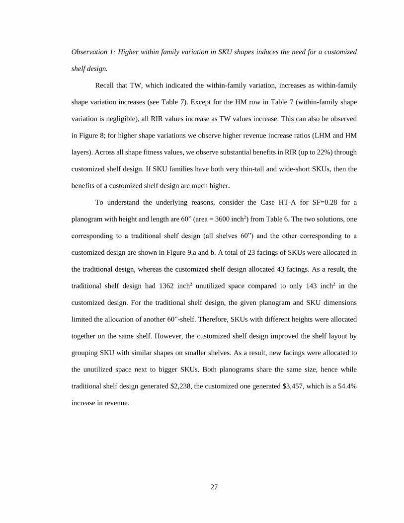
Observation 1: Higher within family variation in SKU shapes induces the need for a customized

shelf design.

Recall that TW, which indicated the within-family variation, increases as within-family

shape variation increases (see Table 7). Except for the HM row in Table 7 (within-family shape

variation is negligible), all RIR values increase as TW values increase. This can also be observed

in Figure 8; for higher shape variations we observe higher revenue increase ratios (LHM and HM

layers). Across all shape fitness values, we observe substantial benefits in RIR (up to 22%) through

customized shelf design. If SKU families have both very thin-tall and wide-short SKUs, then the

benefits of a customized shelf design are much higher.

To understand the underlying reasons, consider the Case HT-A for SF=0.28 for a

planogram with height and length are 60” (area = 3600 inch2) from Table 6. The two solutions, one

corresponding to a traditional shelf design (all shelves 60”) and the other corresponding to a

customized design are shown in Figure 9.a and b. A total of 23 facings of SKUs were allocated in

the traditional design, whereas the customized shelf design allocated 43 facings. As a result, the

traditional shelf design had 1362 inch2 unutilized space compared to only 143 inch2 in the

customized design. For the traditional shelf design, the given planogram and SKU dimensions

limited the allocation of another 60”-shelf. Therefore, SKUs with different heights were allocated

together on the same shelf. However, the customized shelf design improved the shelf layout by

grouping SKU with similar shapes on smaller shelves. As a result, new facings were allocated to

the unutilized space next to bigger SKUs. Both planograms share the same size, hence while

traditional shelf design generated $2,238, the customized one generated $3,457, which is a 54.4%

increase in revenue.

28

Figure 9. SKU arrangement in 60”-shelf and customized shelf designs for SF=0.28 and SF=0.16

Observation 2: As the planogram space fitness increases, shorter shelves become more beneficial,

especially in heterogeneous cases.

Recall that we use SF (space fitness) to quantify the tightness in space of a planogram. So,

in Table 7, across MSL and shape variation values, as SF increases, we observe a general increase

in RIR over the 60” shelf length. While for all HM cases, the increase in RIR of shorter shelves can

be up to 1% as SF increases, for the HT cases, these benefits can increase up to 22%. This is also

evident from Figure 8, where for a fixed point on the Y-axis (SF), we observe a consistent rise in

RIR value as we move from left to right on the X-axis (MSL).

To explain this behavior, consider Case HT-A with SF=0.16 and SF=0.28 (in Table 6). For

SF=0.28, the planogram dimensions are 60” × 60” (total area = 3,600 inch2), while for SF=0.16,

these are 60” × 106” (total area = 6,360 inch2) Figure 9.a and c illustrate the solutions generated by

29

our approach for MSL=12” in both cases. The ratio of the unutilized space to the total planogram

space in Figure 9.a is 0.37 (1362/3600) for SF=0.28, whereas it is 0.24 (1534/6360) for SF=0.16.

Note that, in Figure 9, SKUs 4,6,7,8 and 10 cause unused space. In both SF= 0.28 and SF=0.16

cases for 60"-shelf design, the JSD-SSA model allocates these SKUs at their lower bound facings

to minimize the unutilized space, given that PPI equals $1/inch2. Moreover, in these images, we

also observe that SKUs with higher profitability are allocated more, if possible up to their upper

bound (SKU 9). Therefore, increasing the planogram space (lowering the SF value) increases the

facings of profitable SKUs, while keeping the less profitable SKU facings at their lower bound;

hence decreases the ratio of unutilized space. In other words, higher SF values create higher

unutilized space ratios, which we eliminate by using the JSD-SSA model.

Observation 3: SKUs in the best layouts seem to have a common factor or multiple with other

SKUs and planogram dimensions.

Our results suggested that an allocation of SKUs sharing a common factor or multiple with

the planogram dimensions tend to utilize the planogram space better. To better understand the

common factor, consider height×length of SKUs A and B as 3"×5” and 9"×5”, and that of the

planogram as 9”×10". Because SKUs and the planogram heights share a common factor (3") in

height, the planogram space can be used thoroughly by creating 3 shelves on top of each other for

SKU A and a shelf for B next to SKU-A. Now if SKUs do not share a common factor, the

planogram space can still be completely utilized if they share a common multiple. For instance,

consider height×length of SKUs A and C as 3"×5” and 5"×5”, and that of the planogram as

15”×10". These SKUs and planogram do not share a common factor, but they share a common

multiple (15"); this results in a design with 5 shelves for SKU A on top of each other and 3 shelves

for SKU B on top of each other (next to SKU A), together covering the entire planogram space.

Figure 10 shows the generated planograms for LHM-A and HT-C cases with MSL 12”. Both LHM-

30

A and HT-C have 12 SKUs and 3 families and planogram length, and height is set to 60” and the

total area is 3600 inch2. Notice that LHM-A has SKU lengths and heights, as well as the planogram

length and height, have a common factor of 5 and a common multiple of 30; this is not the case for

HT-C case.

a. LHM-A solution b. HT-C solution

Figure 10. Factors and multiples

The LHM-A solution used all space and generated a maximum revenue of $3600. The

common factor among the SKUs and planograms dimensions was 5. In contrast, the solution for

HT-C (with no clear common factor) resulted in 119 inch2 unutilized space and generated $3481

revenue. Specifically, SKUs 4, 5, 7, 8, and 11 were well-aligned vertically, but not horizontally,

causing 45 inch2 space as unused. Lengths of SKUs 2, 3, 6, and 10 did not have a common multiple

that is smaller than the overall planogram length, as a result, 25 inch2 space was unused. The length

of SKU 0 was a prime number, clearly resulting in a vertical misalignment; 13 inch2 remained

unused. Also due to the height difference between SKU 0 and 9, 13 inch2 area could not be utilized.

These results show that if the dimensions of SKUs do not have a common factor or

multiple, some space tends to stay unutilized. This insight can be useful for retailers for assortment

selection decisions and for negotiating with suppliers on the product packaging as that may affect

planogram space utilization, and thus profitability.

31

6. CASE STUDY

To illustrate the use of our approach, we considered a real planogram at a store of a leading

US retailer in our region and attempted to improve it by using our JSD-SSA model. This existing

planogram has 55 SKUs related to diabetic care, grouped into four families. The price, dimension,

family, and the facings of each SKUs are given in Appendix D. The within and between shape

variations of the planogram are 1067.47 and 1.78. Accordingly, per Chapter 5, we classify this

diabetic care planogram as heterogeneous. The height and width of planogram space are 37” and

52”, respectively, and the LFS is 1029 inch2. The corresponding SF then is 0.53, which is tighter

than all our experimental cases. Figure 11 represents the current and improved layouts for the

diabetic care planogram.

a. Current planogram b. Improved planogram

Figure 11. Shelf design and SKU position for the two planograms

In the current planogram (Figure 11.a), all SKUs have one facing, except for 2 SKUs who

have facings. That is, there are a total of 57 faces. The estimated revenue from this planogram is

$897.9 and the unused space ratio is 0.284.

32

To improve this current planogram, we set the lower bound of facings for all SKUs to 1

and upper bound to 1 more than the current facings. An improved planogram using our PSO-CP

approach is illustrated in Figure 11.b. A few key observations for the improved planogram follow:

• The current planogram uses four 52” shelves, whereas the improved planogram uses five

27” shelves, four 25” shelves, and two 8” shelves. While each family in the current

planogram is assigned on one shelf and distributed vertically, shorter shelves allow better

partitioning of the planogram area in the improved version.

The improved planogram increased the number of SKU faces from 57 to 74 and reduced

the unused space ratio from 0.284 to 0.16 (without reducing the current number of faces). Because

the planogram space fitness value is high (i.e., tight) more facings were assigned to smaller sized

SKUs than larger. The resulting increase in the revenue is 29.2% (from $897.9 to $1160.2).

Additional details can be found in Appendix D.

33

7. CONCLUSION AND FUTURE RESEARCH

Configurable shelves are becoming prominent among a variety of retailers. Configurable

shelves offer retailers the freedom of allocating various sized products together without wasting

the valuable shelf space. This capability can bring competitive advantage to retailers, by enabling

them to create richer assortments within a smaller planogram space. However, it is unclear how

such shelves should be optimally designed and the impact of various product-related factors that

affect such designs.

To this extent, we proposed an optimization-based approach for the joint shelf design and

shelf space allocation problem with the objective of designing a customized shelf layout that

maximizes the space-utilization and revenue. Because of the problem complexity, we resorted to a

decomposition-based approach where we first solve the family area allocation problem (using

particle swarm optimization) and then the SKU assignment problem per family (via Constraint

Programming). In so doing, we proposed a metric to measure the degree of shape diversity of

products and gave guidelines and thresholds for classifying assortments.

Retailers and other industries that allocate items on a storage area, intuitively know that

diversity of shapes requires adjustment of dimension and position of storage units, such as shelves,

bins. One key finding of our study is, it exposes the relation between shape variation, shelf length,

available space, and revenue. Increasing the within-family shape variation can result in higher

revenue increase ratios. Our experiments suggest that for non-homogeneous planograms,

customized shelf designs can increase the revenue can by 22%, based on within family SKU shape

variation level. Through our experiment, we showed that as the space fitness increases the benefits

gained from a customized shelf design also increase. Further, better layout results can be obtained

34

if assortments were constructed in a way that dimensions of SKUs share a common multiple or

factor with both other SKUs and the planogram space. Especially, we observed that avoiding SKUs

with prime number dimensions can reduce the unutilized space, as they fail to align well with other

SKUs.

While our model can handle gondola, peg, bin, and mixed type of shelving, there is room

for further enhancements. First, incorporating vertical and horizontal location effects of an SKU on

customer demand will allow further exploration of the choice of shelf length at each height level

and across the length of the planogram. However, the location effect functions proposed in the

existing literature are nonlinear, and so will add to the complexity of the model. Second, while we

considered that the SKU dimensions provided to us already considered stacking within that SKU,

it is possible to explicitly include them as decision variables in the model. This will allow further

exploration of the effect of various SKU orientations and stacking levels on the choice of shelf

lengths and overall planogram design. Our study considers a 2-level family hierarchy. We believe

the JSD-SSA model can be improved to handle any generic hierarchy structure by borrowing the

modeling approach of Bianchi-Aguiar et al. (2018). It would be interesting to see how location

effects and inventory decisions would impact the shelf design and revenue. Another interesting

extension to our model would be adding the proximity impact on demand for compatible products.

However, introducing these extensions brings more complexity, and we believe that there is a lot

of room for improving the heuristic method for dealing with complexities.

35

REFERENCES

1. Bai, R., & Kendall, G. (2005). An Investigation of Automated Planograms Using a

Simulated Annealing Based Hyper-Heuristic. In Metaheuristics: Progress as Real Problem

Solvers (pp. 87–108). https://doi.org/10.1007/0-387-25383-1_4

2. Bai, R., & Kendall, G. (2008). A Model for Fresh Produce Shelf-Space Allocation and

Inventory Management with Freshness-Condition-Dependent Demand. INFORMS Journal

on Computing, 20(1), 78–85. https://doi.org/10.1287/ijoc.1070.0219

3. Bai, R., van Woensel, T., Kendall, G., & Burke, E. K. (2013). A new model and a hyper-

heuristic approach for two-dimensional shelf space allocation. 4OR, 11(1), 31–55.

https://doi.org/10.1007/s10288-012-0211-2

4. Bianchi-Aguiar, T., Silva, E., Guimarães, L., Carravilla, M. A., & Oliveira, J. F. (2018).

Allocating products on shelves under merchandising rules: Multi-level product families

with display directions. Omega, 76, 47–62. https://doi.org/10.1016/j.omega.2017.04.002

5. Borin, N., Farris, P. W., & Freeland, J. R. (1994). A Model for Determining Retail Product

Category Assortment and Shelf Space Allocation. Decision Sciences, 25(3), 359–384.

https://doi.org/10.1111/j.1540-5915.1994.tb00809.x

6. Brown, W., & Tucker, W. T. (1961). The Marketing Center: Vanishing Shelf Space.

Atlanta Economic Review, October, 9–13.

7. Bultez, A., & Naert, P. (1988). SH.A.R.P.: Shelf Allocation for Retailers’ Profit. Marketing

Science, 7(3), 211–231. https://doi.org/10.1287/mksc.7.3.211

8. Chen, M., & Lin, C. (2007). A data mining approach to product assortment and shelf space

allocation. Expert Systems with Applications, 32(4), 976–986.

36

https://doi.org/10.1016/j.eswa.2006.02.001

9. Corstjens, M., & Doyle, P. (1981). A Model for Optimizing Retail Space Allocations.

Management Science, 27(7), 822–833. https://doi.org/10.1287/mnsc.27.7.822

10. Corstjens, M., & Doyle, P. (1983). A Dynamic Model for Strategically Allocating Retail

Space. Journal of the Operational Research Society, 34(10), 943–951.

https://doi.org/10.1057/jors.1983.207

11. Curhan, R. C. (1972). The Relationship between Shelf Space and Unit Sales in

Supermarkets. Journal of Marketing Research, 9(4), 406. https://doi.org/10.2307/3149304

12. Desgraupes, B. (2018, July 26). CRAN - Package clusterCrit. https://cran.r-

project.org/web/packages/clusterCrit/index.html

13. Drèze, X., Hoch, S. J., & Purk, M. E. (1994). Shelf management and space elasticity.

Journal of Retailing, 70(4), 301–326. https://doi.org/10.1016/0022-4359(94)90002-7

14. Flamand, T., Ghoniem, A., Haouari, M., & Maddah, B. (2018). Integrated assortment

planning and store-wide shelf space allocation: An optimization-based approach. Omega,

81, 134–149. https://doi.org/10.1016/j.omega.2017.10.006

15. Flamand, T., Ghoniem, A., & Maddah, B. (2016). Promoting impulse buying by allocating

retail shelf space to grouped product categories. Journal of the Operational Research

Society, 67(7), 953–969. https://doi.org/10.1057/jors.2015.120

16. Frank, R. E., & Massy, W. F. (1970). Shelf Position and Space Effects on Sales. Journal

of Marketing Research, 7(1), 59–66. https://doi.org/10.1177/002224377000700107

17. Fukunaga, K. (1990). Introduction to statistical pattern recognition (2nd ed.). Academic

Press.

18. Gajjar, H. K., & Adil, G. K. (2011). Heuristics for retail shelf space allocation problem

with linear profit function. International Journal of Retail & Distribution Management,

39(2), 144–155. https://doi.org/10.1108/09590551111109094

19. Geismar, H. N., Dawande, M., Murthi, B. P. S., & Sriskandarajah, C. (2015). Maximizing

37

Revenue Through Two-Dimensional Shelf-Space Allocation. Production and Operations

Management, 24(7), 1148–1163. https://doi.org/10.1111/poms.12316

20. Guthrie, B., & Parikh, P. J. (2020). The rack orientation and curvature problem for retailers.

IISE Transactions, 1–17. https://doi.org/10.1080/24725854.2020.1725253

21. Hansen, J. M., Raut, S., & Swami, S. (2010). Retail Shelf Allocation: A Comparative

Analysis of Heuristic and Meta-Heuristic Approaches. Journal of Retailing, 86(1), 94–105.

https://doi.org/10.1016/j.jretai.2010.01.004

22. Hansen, P., & Heinsbroek, H. (1979). Product selection and space allocation in

supermarkets. European Journal of Operational Research, 3(6), 474–484.

https://doi.org/10.1016/0377-2217(79)90030-4

23. Hariga, M. A., Al-Ahmari, A., & Mohamed, A.-R. A. (2007). A joint optimisation model

for inventory replenishment, product assortment, shelf space and display area allocation

decisions. European Journal of Operational Research, 181(1), 239–251.

https://doi.org/10.1016/j.ejor.2006.06.025

24. Heragu, S. S., & Kusiak, A. (1991). Efficient models for the facility layout problem.

European Journal of Operational Research, 53(1), 1–13. https://doi.org/10.1016/0377-

2217(91)90088-D

25. Hübner, A. H., & Kuhn, H. (2012). Retail category management: State-of-the-art review

of quantitative research and software applications in assortment and shelf space

management. Omega, 40(2), 199–209. https://doi.org/10.1016/j.omega.2011.05.008

26. Hübner, A., & Schaal, K. (2017). A shelf-space optimization model when demand is

stochastic and space-elastic. Omega, 68, 139–154.

https://doi.org/10.1016/j.omega.2016.07.001

27. Hübner, A., Schäfer, F., & Schaal, K. N. (2020). Maximizing Profit via Assortment and

Shelf‐Space Optimization for Two‐Dimensional Shelves. Production and Operations

Management, 29(3), 547–570. https://doi.org/10.1111/poms.13111

38

28. Hwang, H., Choi, B., & Lee, G. (2009). A genetic algorithm approach to an integrated

problem of shelf space design and item allocation. Computers & Industrial Engineering,

56(3), 809–820. https://doi.org/10.1016/j.cie.2008.09.012

29. Hwang, H., Choi, B., & Lee, M.-J. (2005). A model for shelf space allocation and inventory

control considering location and inventory level effects on demand. International Journal

of Production Economics, 97(2), 185–195. https://doi.org/10.1016/j.ijpe.2004.07.003

30. Irion, J, Lu, J.-C., Al-Khayyal, F. A., & Tsao, Y.-C. (2011). A hierarchical decomposition

approach to retail shelf space management and assortment decisions. Journal of the

Operational Research Society, 62(10), 1861–1870. https://doi.org/10.1057/jors.2010.147

31. Irion, Jens, Lu, J.-C., Al-Khayyal, F., & Tsao, Y.-C. (2012). A piecewise linearization

framework for retail shelf space management models. European Journal of Operational

Research, 222(1), 122–136. https://doi.org/10.1016/j.ejor.2012.04.021

32. James V. Miranda, L. (2018). PySwarms: a research toolkit for Particle Swarm

Optimization in Python. The Journal of Open Source Software, 3(21), 433.

https://doi.org/10.21105/joss.00433

33. Kennedy, J., & Eberhart, R. (1995). Particle swarm optimization. Proceedings of ICNN’95

- International Conference on Neural Networks, 4, 1942–1948.

https://doi.org/10.1109/ICNN.1995.488968

34. Kök, A. G., & Fisher, M. L. (2007). Demand Estimation and Assortment Optimization

Under Substitution: Methodology and Application. Operations Research, 55(6), 1001–

1021. https://doi.org/10.1287/opre.1070.0409

35. Lim, A., Rodrigues, B., & Zhang, X. (2004). Metaheuristics with Local Search Techniques

for Retail Shelf-Space Optimization. Management Science, 50(1), 117–131.

https://doi.org/10.1287/mnsc.1030.0165

36. Martello, S., & Toth, P. (1990). Knapsack Problems. John Wiley & Sons Ltd.

37. Montreuil, B. (1991). A Modelling Framework for Integrating Layout Design and flow

39

Network Design (pp. 95–115). https://doi.org/10.1007/978-3-642-84356-3_8

38. Mowrey, C. H., Parikh, P. J., & Gue, K. R. (2018). A model to optimize rack layout in a

retail store. European Journal of Operational Research, 271(3), 1100–1112.

https://doi.org/10.1016/j.ejor.2018.05.062

39. Murray, C. C., Talukdar, D., & Gosavi, A. (2010). Joint Optimization of Product Price,

Display Orientation and Shelf-Space Allocation in Retail Category Management. Journal

of Retailing, 86(2), 125–136. https://doi.org/10.1016/j.jretai.2010.02.008

40. Ozcan, T., & Esnaf, S. (2011). A heuristic approach based on artificial bee colony

algorithm for retail shelf space optimization. 2011 IEEE Congress of Evolutionary

Computation (CEC), 95–101. https://doi.org/10.1109/CEC.2011.5949604

41. Ozcan, T., & Esnaf, Ş. (2016). Swarm Intelligence Approaches to Shelf Space Allocation

Problem with Linear Profit Function (pp. 22–41). https://doi.org/10.4018/978-1-5225-

0075-9.ch002

42. Russell, R. A., & Urban, T. L. (2010). The location and allocation of products and product

families on retail shelves. Annals of Operations Research, 179(1), 131–147.

https://doi.org/10.1007/s10479-008-0450-y

43. Shi, Y., & Eberhart, R. (1998). A modified particle swarm optimizer. 1998 IEEE

International Conference on Evolutionary Computation Proceedings. IEEE World

Congress on Computational Intelligence (Cat. No.98TH8360), 69–73.

https://doi.org/10.1109/ICEC.1998.699146

44. Smith, S. A., & Agrawal, N. (2000). Management of Multi-Item Retail Inventory Systems

with Demand Substitution. Operations Research, 48(1), 50–64.

https://doi.org/10.1287/opre.48.1.50.12443

45. Theodoridis, S. T., & Koutroumbas, K. (2009). Pattern Recognition (4th ed.). Elsevier.

46. Urban, T. L. (1998). An inventory-theoretic approach to product assortment and shelf-

space allocation. Journal of Retailing, 74(1), 15–35. https://doi.org/10.1016/S0022-

40

4359(99)80086-4

47. Urban, T. L. (2002). The interdependence of inventory management and retail shelf

management. International Journal of Physical Distribution & Logistics Management,

32(1), 41–58. https://doi.org/10.1108/09600030210415298

48. van Nierop, E., Fok, D., & Franses, P. H. (2008). Interaction Between Shelf Layout and

Marketing Effectiveness and Its Impact on Optimizing Shelf Arrangements. Marketing

Science, 27(6), 1065–1082. https://doi.org/10.1287/mksc.1080.0365

49. Wirth, M. (2004). Shape Analysis & Measurement Shape Analysis & Measurement. Image

Processing. http://www.cyto.purdue.edu/cdroms/micro2/content/education/wirth10.pdf

50. Yang, M.-H. (2001). An efficient algorithm to allocate shelf space. European Journal of

Operational Research, 131(1), 107–118. https://doi.org/10.1016/S0377-2217(99)00448-8

51. Yang, M.-H., & Chen, W.-C. (1999). A study on shelf space allocation and management.

International Journal of Production Economics, 60–61, 309–317.

https://doi.org/10.1016/S0925-5273(98)00134-0

52. Zufryden, F. S. (1986). A Dynamic Programming Approach for Product Selection and

Supermarket Shelf-Space Allocation. Journal of the Operational Research Society, 37(4),

413–422. https://doi.org/10.1057/jors.1986.69

41

APPENDICES

Appendix A. Comparison of CPLEX and CP performances for subproblem (ii)

For the decomposition-based solution approach described in chapter-4, we tested both the CPLEX

and CP algorithms for the reduced model. Recall that subproblem (ii) would need to be solved

many times, one for each particle in each iteration. To be able to select between the two solvers,

we created 11 cases and compared the solution times and quality (see Table A.1). In the table, Case

Details column, Case, # of family, # of SKU, PW, and PH represent case number, number of

families, planogram length, and planogram height, respectively. Under the CPLEX column, Time,

Best Bound, Obj., and Gap represent solution time, best bound, best integer solution, and the gap

between the best bound and integer solution, respectively. Under the CP column, Time, and Obj,

represent the solution time and the objective function value. Clearly, the performance of CP was

far more superior than CPLEX in solving the subproblem (ii).

Table A.1. CPLEX and CP performance comparison in solving subproblem (ii)

Case Details CPLEX CP

Case # of

Family

# of

SKU PW PH

Time

(sec)

Best

Bound Obj Gap

Time

(Sec) Obj

1 1 30 60 72 >9000 - - - 119 1399

2 1 30 30 72 >9000 1130 1071 6% 70 966

3 2 9 30 72 >1800 820 676 21% 10 650

4 1 45 30 72 >1800 429 - - 119 405

5 2 24 30 72 >1800 429.8 392 9.25% 83 413

6 0 34 30 72 >1800 636 - - 160 484

7 1 4 24 24 >1800 332 120 175% 0.5 120

8 1 4 48 48 >1800 603 483 25.00% 1.5 483

9 2 26 30 72 >1800 828 751 10% 35 766

10 2 26 60 72 >1800 1998 - - 120 1590

11 4 3 15 15 381 71 71 0% 0.3 71

42

In table A.1 Case Details column, Case, # of family, # of SKU, PW, and PH represent case number,

number of families, planogram length, and planogram height respectively. In the CPLEX column,

Time, Best Bound, Obj., and Gap represent solution time, best bound, best integer solution, and the

gap between the best bound and integer solution respectively. In CP column Time, and Obj,

represent the solution time and the objective function value.

43

Appendix B. PSO-CP Convergence Table

We tested the convergence of the PSO-CP algorithm in 3 cases. We solved each case 3 times using 6 particles and recorded global best solutions

and particle best solutions and represent them in Table B.1.

Table B.1. PSO -CP Convergence

Case Name Runs

Objective Value of Particles Global

Best

MAPE Between

P-1 P-2 P-3 P-4 P-5 P-6 Particles Runs

N5F2W24H60

1 97.27 97.27 97.27 97.27 97.27 97.27 97.27 0 % 0 %

2 97.27 97.27 97.27 97.27 97.27 97.27 97.27 0 % 0 %

3 97.27 97.27 97.27 97.27 97.27 97.27 97.27 0 % 0 %

N10F2W36H72

1 221.92 221.92 221.92 221.92 222.59 221.92 222.59 0.25 % 0 %

2 221.92 221.92 221.92 221.92 221.92 221.92 221.92 0 % 0.3%

3 221.92 221.92 222.59 222.59 222.59 221.92 222.59 0.15 % 0 %

N10F3W36H72

1 255.4 255.4 255.4 255.4 255.4 255.4 255.4 0 % 0 %

2 255.4 255.4 255.4 255.4 255.4 255.4 255.4 0 % 0 %

3 255.4 255.4 255.4 255.4 255.4 255.4 255.4 0 % 0 %

Average 0.04% 0.03

In Table B.1 MAPE represents the Mean Absolute Percentage Error between particles and between runs. Table B.1 shows that the average MAPE

between particles was 0.04% and the average MAPE between global best objective function values was 0.03%.

44

Appendix C. Experiment Results

Table C.1 shows the details of the test-runs completed for shape variation and space fitness experiments.

Table C.1. Experiment Results

(Note: For each case, the first row indicates revenue in $ and the second row indicates run time in seconds.)

SF = 0.28 (PW:60, PH:60) SF = 0.23 (PW:72, PH:60) SF = 0.20 (PW:84, PH:60) SF = 0.16 (PW:106, PH:60)

Case Min Shelf Length Min Shelf Length Min Shelf Length Min Shelf Length

12” 24” 36” 48” 60” 12” 24” 36” 48” 60” 12” 24” 36” 48” 60” 12” 24” 36” 48” 60”

HM-A 3351 3351 3351 3351 3351 4191 4191 4191 4191 4191 4779 4779 4779 4779 4779 5871 5871 5871 5871 5871

1187 782 743 623 893 1236 977 882 1015 1099 1262 912 859 805 1016 1103 1118 960 876 860

HM-B 3351 3340 3276 3276 3276 3950 3938 3928 3928 3928 4632 4576 4576 4576 4576 5778 5778 5764 5764 5764

864 607 30 26 15 735 233 16 26 34 748 119 17 15 26 1007 518 32 37 21

HM-C 3560 3560 3560 3560 3560 3740 3740 3740 3740 3740 4760 4760 4760 4760 4760 5960 5960 5960 5960 5960

747 698 598 609 787 688 617 418 458 588 668 794 621 685 970 720 653 503 526 536

HM-D 3600 3600 3600 3600 3600 3600 3600 3600 3600 3600 4500 4500 4500 4500 4500 6180 6180 6180 6180 6180

698 691 539 504 1113 1514 969 1087 728 723 987 943 921 815 1289 1252 1066 1124 1005 1675

LHM-A 3600 3600 3300 3300 3300 4150 4100 4100 3850 3850 4750 4700 4650 4650 4650 6150 6150 6150 6150 6150

1176 1191 109 153 36 560 228 491 93 23 612 297 171 209 583 836 154 60 14 20

LHM-B 3287 3277 3203 3203 3203 4011 3900 3807 3780 3780 4680 4644 4608 4375 4375 6034 5950 5875 5861 5785

398 134 354 15 9 1088 177 21 22 15 185 88 7 12 13 91 32 28 181 15

LHM-C 3297 3297 3270 3270 3270 4092 3855 3855 3855 3855 4526 4490 4454 4346 4346 4950 4950 4950 4950 4860

1357 78 14 23 100 438 387 49 114 113 214 63 76 17 15 526 297 35 232 33

LHM-D 3376 3245 3173 3173 3173 4104 4098 4092 3989 3989 4403 4403 4385 4339 4339 5812 5471 5486 5486 5369

1711 363 35 45 85 705 820 315 107 110 65 191 87 124 426 1797 1374 61 93 66

HT-A 3457 3449 2238 2238 2238 4161 4127 4089 2960 2960 4913 4823 4757 3610 3610 6255 6133 6164 6122 4826

1271 737 119 68 116 1687 2235 738 69 59 1829 1383 1146 56 36 1946 1833 1347 1489 66

HT-B 3468 3365 3094 3094 3094 4124 4011 3987 3647 3647 4811 4762 4630 4337 4337 6070 5984 5859 5859 5801

1278 1357 879 705 740 1412 1198 2200 887 1134 1754 1685 1797 1099 1882 1789 1782 1645 2844 1738

HT-C 3481 3367 3083 3083 3083 4219 4166 3910 3767 3767 4759 4719 4615 4471 4471 6031 6039 5907 5901 5507

2219 1747 682 641 1557 1751 1872 1972 744 774 1677 2407 1553 831 1312 2053 3089 1621 2728 1699

HT-D 3369 3345 3083 3083 3083 4135 4052 3910 3767 3767 4890 4783 4753 4471 4471 6134 6059 5992 5500 5301

1373 2063 667 686 753 1734 1731 2475 1077 633 2690 1878 2439 1096 1927 1811 3119 2272 1779 1736

45

Appendix D. Case Study Results

In Table D.1, columns W, H represents the width and height of each SKU. The family and

price of each SKU are given in Family and P columns. Org. face column represents the number of

faces in the original planogram. Columns Lower and Upper show the lower and upper bounds for

the number of faces. The number of faces created by the improved design is represented in Imp.

face column. We also represent the area of each SKU in the Area column.

Table D.1 shows that the highest increase in the number of faces is in family 1. Note that

in family 1, SKU sizes are smaller compared to other families. PSO-CP was able to utilize the

previously unused space by increasing the facings of smaller products and grouping them on a

separate shelf. We also observe that even though the SKU prices are lower in family 1, the PSO-

CP model still preferred to allocate more from family 1. It seems like SKU dimensions have more

impact on revenue than SKU prices for this planogram. These observations show that a greedy

SKU allocation can result in a sub-optimal design.

46

Table D.1. Case study data and results

UPC W H Family P ($) Org. face Lower Upper Imp. face Area

1 2 3 1 15.99 1 1 2 2 6

2 5 7 3 24.99 1 1 2 1 35

3 5 8 4 29.99 1 1 2 1 40

4 3 4 1 10.99 1 1 2 2 12

5 5 7 4 19.99 1 1 2 1 35

6 2 2 2 39.99 1 1 2 1 4

7 6 3 1 1.99 2 1 3 3 18

8 3 5 2 3.99 1 1 2 1 15

9 3 5 1 14.99 1 1 2 2 15

10 2 3 2 25.92 1 1 2 2 6

11 4 6 4 29.99 1 1 2 1 24

12 4 4 3 2.99 1 1 2 2 16

13 3 5 2 11.99 1 1 2 1 15

14 5 7 4 29.99 1 1 2 1 35

15 3 4 1 1.99 1 1 2 1 12

16 2 5 1 13.99 1 1 2 2 10

17 3 2 2 34.99 1 1 2 1 6

18 3 5 2 3.99 1 1 2 1 15

19 5 7 4 19.99 1 1 2 1 35

20 4 6 2 19.99 1 1 2 1 24

21 2 2 2 34.99 1 1 2 1 4

22 4 2 3 1.99 1 1 2 2 8

23 3 4 2 1 1 1 2 1 12

24 4 6 3 34.99 1 1 2 1 24

25 5 7 4 34.99 1 1 2 1 35

26 4 6 3 34.63 1 1 2 1 24

27 4 6 4 29.99 1 1 2 2 24

28 3 4 1 1.99 1 1 2 1 12

29 4 6 3 30.99 1 1 2 1 24

30 3 5 2 7.99 1 1 2 1 15

31 2 3 1 15.99 1 1 2 2 6

32 3 3 1 11.99 1 1 2 2 9

33 3 4 2 1 1 1 2 1 12

34 3 3 1 7.99 1 1 2 2 9

35 3 4 2 1 1 1 2 1 12

36 4 8 3 3.99 1 1 2 1 32

37 5 7 3 19.99 1 1 2 1 35

38 3 3 1 43.5 1 1 2 2 9

39 5 7 4 9.49 1 1 2 1 35

40 3 4 1 1.99 1 1 2 1 12

41 6 3 1 1.99 2 1 3 2 18

42 3 4 1 11.99 1 1 2 2 12

43 5 7 4 19.99 1 1 2 1 35

44 2 4 1 11.99 1 1 2 2 8

45 3 5 2 3.99 1 1 2 1 15

46 5 7 3 19.99 1 1 2 1 35

47 3 4 1 1.07 1 1 2 1 12

48 3 5 2 8.7 1 1 2 1 15

49 4 6 2 9.99 1 1 2 1 24

50 4 6 3 21.09 1 1 2 1 24

51 3 5 2 3.99 1 1 2 1 15

52 2 2 2 19.99 1 1 2 1 4

53 2 2 2 21.99 1 1 2 2 4

54 6 7 4 27.99 1 1 2 1 42

55 5 7 3 19.99 1 1 2 1 35

joint shelf design and shelf space allocation problem for

Documents