Portland State University Portland State University

PDXScholar PDXScholar

Computer Science Faculty Publications and Presentations Computer Science

2019

Joint Stabilization and Direction of 360° Videos Joint Stabilization and Direction of 360° Videos

Chengzhou Tang Simon Fraser University

Oliver Wang Adobe Systems Inc

Feng Liu Portland State University, fliu@pdx.edu

Ping Tan Simon Fraser University

Follow this and additional works at: https://pdxscholar.library.pdx.edu/compsci_fac

Part of the Computer Sciences Commons

Let us know how access to this document benefits you.

Citation Details Citation Details Tang, Chengzhou; Wang, Oliver; Liu, Feng; and Tan, Ping, "Joint Stabilization and Direction of 360° Videos" (2019). Computer Science Faculty Publications and Presentations. 204. https://pdxscholar.library.pdx.edu/compsci_fac/204

This Pre-Print is brought to you for free and open access. It has been accepted for inclusion in Computer Science Faculty Publications and Presentations by an authorized administrator of PDXScholar. Please contact us if we can make this document more accessible: pdxscholar@pdx.edu.

Joint Stabilization and Direction of 360◦ Videos

CHENGZHOU TANG, Simon Fraser UniversityOLIVER WANG, Adobe Systems IncFENG LIU, Portland State UniversityPING TAN, Simon Fraser University

360◦ video provides an immersive experience for viewers, allowing themto freely explore the world by turning their head. However, creating high-quality 360◦ video content can be challenging, as viewersmaymiss importantevents by looking in the wrong direction, or they may see things that ruin theimmersion, such as stitching artifacts and the film crew.We take advantage ofthe fact that not all directions are equally likely to be observed; most viewersare more likely to see content located at “true north”, i.e. in front of them,due to ergonomic constraints. We therefore propose 360◦ video direction,where the video is jointly optimized to orient important events to the front ofthe viewer and visual clutter behind them, while producing smooth cameramotion. Unlike traditional video, viewers can still explore the space as desired,but with the knowledge that the most important content is likely to be infront of them. Constraints can be user guided, either added directly on theequirectangular projection or by recording “guidance” viewing directionswhile watching the video in a VR headset, or automatically computed, suchas via visual saliency or forward motion direction. To accomplish this,we propose a new motion estimation technique specifically designed for360◦ video which outperforms the commonly used 5-point algorithm onwide angle video. We additionally formulate the direction problem as anoptimization where a novel parametrization of spherical warping allows usto correct for some degree of parallax effects. We compare our approach torecent methods that address stabilization-only and converting 360◦ videoto narrow field-of-view video. Our pipeline can also enable the viewing ofwide angle non-360◦ footage in a spherical 360◦ space, giving an immersive“virtual cinema” experience for a wide range of existing content filmed withfirst-person cameras.

CCS Concepts: • Computing methodologies → Image manipulation; Computational photography;

Additional Key Words and Phrases: VR, 360 video, re-cinematography, video stabilization

1 INTRODUCTIONVR headsets are rapidly gaining in popularity, and one of the mostcommon use cases is viewing 360° videos, which provide addedimmersion due to the ability of the viewer to explore a wider fieldof view than traditional videos. However, this freedom introduces anumber of challenges for content creators and viewers alike; viewerscan miss important events by looking in the wrong direction, or

they can see things that break immersion, such as stitching artifactsor the camera crew.In this work, we address two important aspects of 360 video

creation; direction of shots to draw the viewers’ attention to desiredregions, and smooth, intentional camera trajectories. Both of theseparts are crucial in 360◦ video; viewer freedom makes directionchallenging, and unstablemotion (especially in the peripheral vision)can be disorienting, causing confusion and even nausea [Jerald2016]. While traditional cinematography refers to the decisionsmade during filming, 360◦ video is particularly well suited to thetask of modifying the camera direction in post (also known as re-cinematography [Gleicher and Liu 2008]), as all viewing directionsare recorded at capture time, giving us greater control in post.

We therefore propose amethod that uses direction constraints [Gandhiet al. 2014] (e.g., where to look, where not to look), that try to keepdesirable content in the viewable space near true-north, and unde-sirable content largely behind the user. These are jointly optimizedwith smoothness constraints that reduce camera shake and rapidrotations, such as those caused by hand held cameras, motorizedgimbals, or inconsistent direction constraints. We allow an editorto manually define desirable and undesirable regions in the video,as well as the ability to use automatically derived constraints suchas saliency maps, forward motion, or stitching regions for knowncamera configurations. In the case of manual constraints, editorscan either directly draw on the equirectangular projection, or alter-nately we propose a new type of interaction where the editor viewsthe content in a VR headset as a “guide”, and their viewing path isrecorded and used as a constraint in the joint optimization.In summary, we propose a solution for joint stabilization and

direction of 360◦ videos, where undesirable camera motions (e.g.,shake and rapid rotations) are removed while following a smoothand directed camera path. Our solution also works for wide-anglevideos, enabling “virtual cinema” viewing in VR for a large libraryof existing footage. To achieve these goals, we present the followingtechnical contributions:

• A motion estimation algorithm based on non-linear optimiza-tion which performs better than widely used five-point algo-rithm on 360◦ and wide-angle videos.

• A 3D spherical warping model derived from our motion esti-mation that and handles both rotation and translation whichallows more control than the recently proposed method [Kopf2016].

• A unified framework to define and add constraints from dif-ferent sources on the resulting 360◦ video, including a newVR interface and automatic motion constraints.

To validate these contributions, we make both qualitative and quan-titative comparisons and conduct user study to show that in our

arX

iv:1

901.

0416

1v1

[cs

.GR

] 1

4 Ja

n 20

19

1:2 • Tang, C. et al

Fig. 1. Our method follows the above pipeline; features are tracked across all frames, after which keyframes are selected. A novel 3D camera motion estimationis combined with user-guided viewing constraints in the path planning step to produce a set of aligned keyframes, and the results are finally interpolated ontoall frames of the video. 360◦ frames are visualized as rectangles.

directed results, viewers are much more likely to observe the desiredparts of the sequence marked with positive constraints.

2 RELATED WORK360◦ video can now be captured by both consumer handheld cam-eras, such as Ricoh Theta, Nikon KeyMission, and Kodak PixproSP360, and professional camera array systems [Anderson et al. 2016;Lee et al. 2016]. The captured 360◦ video often needs to be post-processed to deliver a pleasant viewing experience. We briefly re-view relevant prior research.

Video stabilization is a common approach to improve the cameramotion of a video. Common ways to stabilize video involve trackingfeatures over time and computing an image warp sequence thatsmooths feature trajectories and thus the apparent motion of thevideo. This can be achieved by applying a sequence of homographiesor other 2D transformations that compensate the motion [Chen et al.2008; Lee et al. 2009; Matsushita et al. 2006], by using a grid of ho-mographies [Liu et al. 2013] for robustness, by using projectivereconstruction [Goldstein and Fattal 2012], on a low dimensionalfeature subspace [Liu et al. 2011], as used in Adobe After Effects, orby fitting smooth cropping windows that minimize first and secondorder motion [Grundmann et al. 2011], as used on YouTube. Alter-nate approaches have proposed building a full 3D reconstruction ofthe scene, which can be used to synthesize a smooth virtual cameratrajectory [Buehler et al. 2001; Kopf et al. 2014; Liu et al. 2009].

Recently, Kopf [2016] presented an extension of video stabilizationto 360◦ videos. This approach computes a 3D geometric relationshipbetween keyframes via the 5-point algorithm [Li and Hartley 2006],and smoothly interpolates keyframes using a deformable model. Weuse a similar approach with a few significant modifications.WhereasKopf [2016] is largely used to compute a “total” stabilization (wherefixed scene points will remain stationary throughout the video),we go beyond stabilization and combine artistic and smoothnessconstraints to produce an easy to watch 360◦ video with directedcamera motion. One requirement to support this goal is that weneed a full 3D motion rotation and translation estimation per frame.To achieve this, we introduce a new method for estimating rotation

and translation on a sphere that is more robust than the 5-pointalgorithm.

Ourwork is inspired by previouswork on re-cinematography [Gandhiet al. 2014; Gleicher and Liu 2008], where casually captured videois improved by integrating high-level content driven constraintsand low-level camera motion stabilization. We extend this notion to360◦ video, which benefits from all viewing angles being capturedduring filming, so cropping is not necessary, freeing our methodfrom the trade off between guiding the viewer’s attention and pre-serving video content. Similar path planning in traditional videohas also been used for retargeting [Jain et al. 2015; Wang et al. 2009],which distorts or crops off less important content to fit the videointo a different aspect ratio other than originally intended.The Pano2Vid work by Su et al. [2016] performs a related, but

different task of automatically producing a narrow field-of-viewvideo from a 360◦ video. A recent follow-up work extended this tooptimize for zoom as well [Su and Grauman 2017]. These approachesare complementary to ours; in our work, we combine viewing con-straints with motion estimation to compute smooth directed camerapaths for 360◦ viewing. Pano2Vid presents a learning based saliencycomputation, and computes a shortest path on these values. As itdoes not perform any motion estimation, it cannot be used to sta-bilize camera motion in shaky videos. We show that we can usethe output from Pano2Vid as automatic saliency constraints for ourmethod, which generates smooth camera paths where importantcontent is placed in front of the viewers.

One of our main assumptions is that by rotating important objectsin front of viewers, VR viewing becomes a more enjoyable experi-ence. This is in some sense, reducing some control of the viewer tofreely explore the space, as some rotations will be out of the controlof the viewer. Whether this kind of motion is “allowable” is an opentopic in VR film making, but we note that traditional wide anglevideo also started with static shots before filmmakers learned howto use camera motion as an artistic tool without disorienting theviewer/

In this domain, work by Sun et al. [2016] has shown that it isin fact possible to separate the viewer’s real world head motionfrom the perceived motion in the VR space in order to map virtual

Joint Stabilization and Direction of 360◦ Videos • 1:3

spaces into physical constraints such as room sizes without causingconfusion. Sitzmann et al. [2018] also conducted user studies andconcluded that the faster user attention gets directed towards thesalient regions, the more concentrated their attention is.

3 METHODFigure 1 provides an overview of the approach. We first estimatethe existing motion between keyframes using feature tracking and anovel pairwisemotion estimation formulation for spherical andwideangle video. We then solve a joint optimization on the keyframesthat enforces smoothness in the warped video sequence and a setof user-provided (or automatic) path planning constraints. Finally,we smoothly interpolate the motion between keyframes to producethe final output video. We now discuss each step in more detail.

3.1 Feature Tracking and Keyframe SelectionSimilar to prior work [Kopf 2016], for 360◦ videos we remap theequirectangular image to a cube map and track feature points inde-pendently on each cube face using KLT feature tracking [Shi andTomasi 1994]. For wide-angle videos, we perform the tracking di-rectly on the video frames. This is the only stage of the process thatis different between 360◦ and traditional wide-angle video, aftertracking we project feature points onto a sphere and treat both typesof videos identically. In the following, we will use unit vector p todenote the projected points on a sphere.

Similar to other approaches, we select feature points on keyframesand track them through the video [Kopf 2016; Kopf et al. 2014]. Thefirst and last frames are selected as keyframes, and we create newkeyframes every time the percentage of successful tracked featuresdrops to 60% of the number of features initially detected. Finally,we only select feature points that are more than 2◦ away from anypreviously selected feature points.After feature tracking, we have a set of m feature trajectories

T = {Ti |i = 1 · · ·m} through the video, where each trajectory Ti isa list of points from several continuous frames:

Ti = {pij |j = si · · · ei }, (1)

where si is the starting frame (which is always a keyframe), and eiis the last keyframe where the point was successfully tracked.

3.2 Rotation and Translation EstimationAfter collecting feature tracks, we estimate the relative 3D rotationand translation between neighboring pairs of keyframes. A com-mon solution is to use the 5-point algorithm [Nister 2004], to firstestimate the essential matrix, decompose it into a rotation matrixR and a translation direction vector t, and then improve the esti-mated motion by iterative refinement [Triggs et al. 2000]. With thisapproach, the final quality relies on the accuracy of the essentialmatrix estimation as well as the motion decomposition. It is wellknown both of these steps are highly dependent on the quality of thecamera calibration [Stewenius et al. 2005], feature trajectories, andglobal shutter camera [Dai et al. 2016]. As a result, prior 360◦ stabi-lization work only uses the estimated rotation between neighboring

!p

r

p0

(a) Rotation

p

t⇥p

t

p0✓

(b) Translation

tq

p0Rp

t⇥Rp

EM✓

(c) Combined

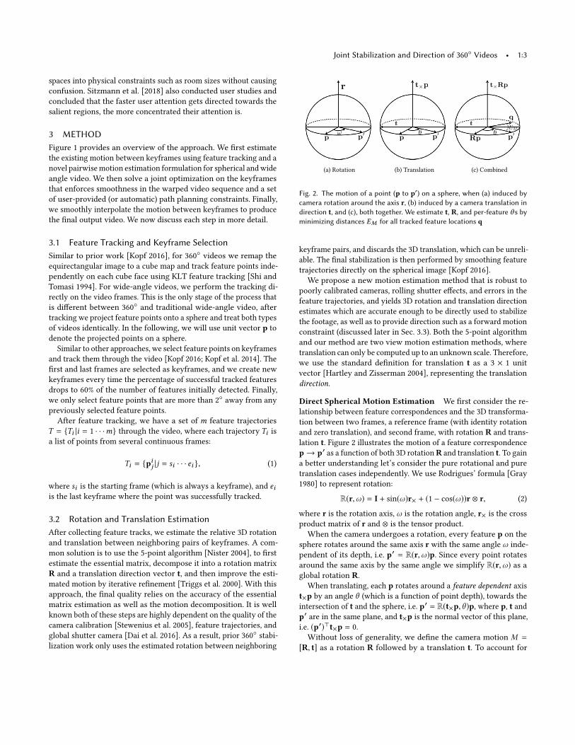
Fig. 2. The motion of a point (p to p′) on a sphere, when (a) induced bycamera rotation around the axis r, (b) induced by a camera translation indirection t, and (c), both together. We estimate t, R, and per-feature θ s byminimizing distances EM for all tracked feature locations q

keyframe pairs, and discards the 3D translation, which can be unreli-able. The final stabilization is then performed by smoothing featuretrajectories directly on the spherical image [Kopf 2016].We propose a new motion estimation method that is robust to

poorly calibrated cameras, rolling shutter effects, and errors in thefeature trajectories, and yields 3D rotation and translation directionestimates which are accurate enough to be directly used to stabilizethe footage, as well as to provide direction such as a forward motionconstraint (discussed later in Sec. 3.3). Both the 5-point algorithmand our method are two view motion estimation methods, wheretranslation can only be computed up to an unknown scale. Therefore,we use the standard definition for translation t as a 3 × 1 unitvector [Hartley and Zisserman 2004], representing the translationdirection.

Direct Spherical Motion Estimation We first consider the re-lationship between feature correspondences and the 3D transforma-tion between two frames, a reference frame (with identity rotationand zero translation), and second frame, with rotation R and trans-lation t. Figure 2 illustrates the motion of a feature correspondencep → p′ as a function of both 3D rotationR and translation t. To gaina better understanding let’s consider the pure rotational and puretranslation cases independently. We use Rodrigues’ formula [Gray1980] to represent rotation:

R(r,ω) = I + sin(ω)r× + (1 − cos(ω))r ⊗ r, (2)

where r is the rotation axis, ω is the rotation angle, r× is the crossproduct matrix of r and ⊗ is the tensor product.When the camera undergoes a rotation, every feature p on the

sphere rotates around the same axis r with the same angle ω inde-pendent of its depth, i.e. p′ = R(r,ω)p. Since every point rotatesaround the same axis by the same angle we simplify R(r,ω) as aglobal rotation R.

When translating, each p rotates around a feature dependent axist×p by an angle θ (which is a function of point depth), towards theintersection of t and the sphere, i.e. p′ = R(t×p,θ )p, where p, t andp′ are in the same plane, and t×p is the normal vector of this plane,i.e. (p′)⊤t×p = 0.Without loss of generality, we define the camera motion M =

[R, t] as a rotation R followed by a translation t. To account for

1:4 • Tang, C. et al

noise in the feature tracks, we estimate the rotation R, translationt and the feature dependent angle θ by minimizing the followingerror where q is the tracked feature location:

EM (R, t,θ ) = ∥q − p′∥2 = ∥q − R(t×Rp,θ )Rp∥2 (3)

over all feature correspondences between two keyframes. This en-ergy measures the Euclidean distance between q and p′ where p′ isthe point found by rotating p with R and then with R(t×Rp,θ ). Weobserve that the energy in Eq. 3 is hard to optimize directly becauseof the point-dependent angle θ . In practice, there are about 3000 fea-ture correspondences between two frames and each correspondencehas an θ , which gives a large amount of unknowns.

Instead, we directly estimate the rotation and translation betweentwo frames by first ignoring θ , and minimizing the least squareserror:

EM (R, t) = ∥ arcsin(q⊤t×Rp∥t×Rp∥

)∥2 (4)

over all feature correspondences. Eq. 4 is a function of R(threeDoFs) and t(three DoFs), which is much easier to solve then Eq. 3.As shown in Fig 2, Eq. 4 measures the angular distance between thetracked point q and the plane that contains Rp and t, which is alsothe angular distance between q and p′.

We can then compute θ by projecting q onto the same plane withRp and t, giving the projection as p′, and then measure the angulardistance between p and p′ as θ . We found it to be unnecessary toconstrain t to be a unit vector during the optimization, as Eq. 4 isalready normalized, and the scale of t does not affect the value ofEM . We therefore only normalize t after the optimization is finished.Before minimizing Eq. 4, we identify inlier feature correspon-

dences using RANSAC with the fundamental matrix as a model,estimated by the 7-point algorithm [Hartley and Zisserman 2004].The reason for not choosing the more often used 8-point algorithmis that the normalization in 8-point algorithm is inapplicable tospherical points, and the 7-point algorithm is more efficient in thepresence of noise. While the fundamental matrix is unable to giveus the rotation and translation directly, it is helpful to identify fea-ture tracks inconsistent with possible camera motion, especially forscenes with moving objects.

We now can compute the relative motionMi,i+1 = [Ri,i+1, ti,i+1]between all neighboring pairs of keyframes ki → ki+1 by minimiz-ing Eq. 4 using a non-linear least squares solver. We then chainrotations to align each keyframe in a global coordinate frame (e.g.,that of the first keyframe):

Rki =

i−1∏j=1

Rkj ,kj+1 . (5)

We use the relative translation direction tki ,ki+1 to compute the finalwarped frames and for the forward motion constraint.

We then compute the relative camera motion for all remainingframes between a given pair of keyframes ki and ki+1. To do this,we set the neighboring keyframes to be the reference frame, andseparately solve for the in-between frame by minimizing Eq. (4),averaging the result from both nearest keyframes (previous andnext). We evaluate the results both qualitatively and quantitativelyin Sec 4.

3.3 Joint Stabilization and DirectionNow that we have estimated the input camera path, we are ableto define our joint stabilization and direction optimization, whichconsists of two terms:

E(W ) = Ed (W ) + Es (W ), (6)

where Ed is an energy that captures directional constraints andEs encourages the smoothness in the resulting spherical video.Wis a set of camera transformations that correspond to the optimal(virtual) camera trajectory. In this optimization, we use a combinedrotation and translation model W to transform the input video,which we render using image warping.

We first solve Eq. 6 consideringW restricted to rotation only andthen later solve the two terms Ed (W ) and Es (W ) considering modelsthat handle both rotation and translation. In the following twosections, and implementation, we present rotation in quaternions.

3.4 Directional ConstraintsDirectional constraints can be either positive, which specify salientevents that the editor would like viewers to see, or negative, in-dicating things that should not be seen, for example content thatis uninteresting, that contains elements that do not belong in thescene, such as the camera crew, or stitching seams. Fig. 3 shows thevarious types of constraints we use.

Source of Constraints We provide two types of user providedconstraints. In one case, the editor simply clicks directly on theER projection, while in the other, the editor provided a “guided”viewing session, where they watch the video in a VR headset, andtheir viewing direction is recorded over time, and used as positiveconstraints. To support this, we developed an app that records theusers head rotation during the playback of a video in a GoogleCardboard headset. This trajectory is then sampled at every secondand used in our optimization to guide the look-at direction over thecourse of the video.Our method can also be easily integrated with automatically

generated constraints. Automatic saliency methods for 360◦ video(e.g., [Su et al. 2016]) determine the most visually salient regions,which can be directly interpreted as positive constraints. Alternately,as we are estimating 3D translation direction in Section 3.2, we canuse this to keep the camera pointed roughly in the forward mo-tion direction, which provides a comfortable “first-person” viewingexperience. Automatic negative constraints can also be added, forexample for seam locations if the camera geometry is known a priori.We show examples of all of these types of constraints in the resultsection and supplemental material.

Constraint Formulation A positive constraint is represented asa look-at point pi located on a spherical video frame fi . The goal isto transform the frame fi by a rotation quaternion qWfi such that piis as close to the true north direction as possible, thereby making itmore likely to be seen. Similarly, a negative constraint nj locatedon frame fj is one that we want to avoid appearing in the front,i.e., we search for a transformation qWfj to make this point appearoutside of the user’s likely viewing direction.

Joint Stabilization and Direction of 360◦ Videos • 1:5

(a) (b) (c) (d)

Fig. 3. Our method can be used with a variety of input sources. Here we show some ways to provide directional constraints. A user can manually selectregions on an ER projection (left), or create a guided viewing experience in a VR headset (b), or we can use automatic constraints such as saliency e.g., [Su et al.2016] (c), or from forward motion (Sec. 3.2) (d).

L2 Loss Our Loss for Negative Constraints

Fig. 4. L2 loss vs. robust loss for negative constraints. We make the penaltyclose to zero as long as the negative constraint is out of visible region, andthe penalty increases sharply when the negative constraint moves towardsvisible region. The forward direction is marked as blue arrows.

Therefore, for a set P of positive constraints, and N of negativeconstraints, the directional term can be expressed as:

Ed (W ) =∑i ∈P

∥qWfi · pi − f∥22 +∑j ∈N

ρ(∥qWfj · nj − b∥22 ), (7)

where qWfi · pi denotes rotating pi by quaternion qWfi , and qWfiminimizes the distance betweenpi and the front vector f = [0, 0, 1]⊤,and qWfj maximizes the distance of nj to the front vector f, whichis equivalent to minimizing the distance to the back vector b =[0, 0,−1]⊤.

Because we may only want the negative constraint to be outsidethe of view (rather than exactly behind the user), we use a robust lossfunction ρ(x) = αe−

βx on the negative constraint. We set α = 3200

and β = 26.73, which causes ρ(x) to yield a low cost until it enters avisible region for the average human field of view (which is roughly114°horizontally [Strasburger et al. 2011]), after which the penaltyincreases sharply, as shown in Fig. 4.

3.5 Smoothness ConstraintsFrom Sec. 3.2, we have computed the global rotation Ri for allframes, with respect to the first frame. We use a smoothness modelsimilar to [Kopf 2016], but with small modifications. Importantly, wedefine the first-order and second-order smoothness terms directlyon the estimated camera rotations instead of the feature trajectories,

i.e.,Es (W ) = α1Es1(W ) + α2Es2(W ), (8)

where

Es1(W ) =n−1∑i=1

���qWi+1qi+1 − qWi qi���p

(9)

is the first order term and,

Es2(W ) =n−2∑i=1

���(qWi+2qi+2)−1qWi+1qi+1 − (qWi+1qi+1)−1qWi qi

���p,

(10)is the second order term.This energy is summed over all n frames, and |qa − qb | is the

difference between two quaternion rotations, α1 and α2 are weights,and p is the norm of the smoothness that we solve for. In our imple-mentation, we use α1 = 10 and α2 = 100 for all results shown, butthese values could be changed to control the trade-off between thedirection constraints and video smoothness.

3.6 OptimizationWe can now directly minimize Eq. 6 using the Levenberg-Marquardtalgorithm in Ceres and achieve a final rotation-only directed video.However, for efficiency, we propose the following optimizationscheme which gradually propagates a good initialization, speedingup convergence.We also observe that some axes of rotation can be confusing

for the viewer. In particular, camera movement in the roll axis isuncommon in many videos recorded on a ground plane, and canbe confusing. We therefore default to fixing the roll axis inψ andallow for rotation only in the pitch and yaw of the camera, unlessotherwise specified by the user (for example in the wing-suit video(Fig. 17), we enable rotation on the roll axis).

We can choose between smoothness norms in our optimization,in particular prior works have used L1 and L2 norms. Using an L1norm tends to give clear distinctions between fixed and movingshots, while L2 paths are smoother overall. We provide examplesof L1 and L2 smoothed paths in the supplemental material, andallow the user to choose which norm (p = 1 or p = 2) they want tominimize.

3.7 Translation-Aware TransformationUntil now, we have considered rotation-only transformation forW ,which have the advantage of being quick to compute, as there are

1:6 • Tang, C. et al

P

pj Rijpi

�

!

d

kifjtij

P

pj

tWj

!

fj fWj

RWj wj

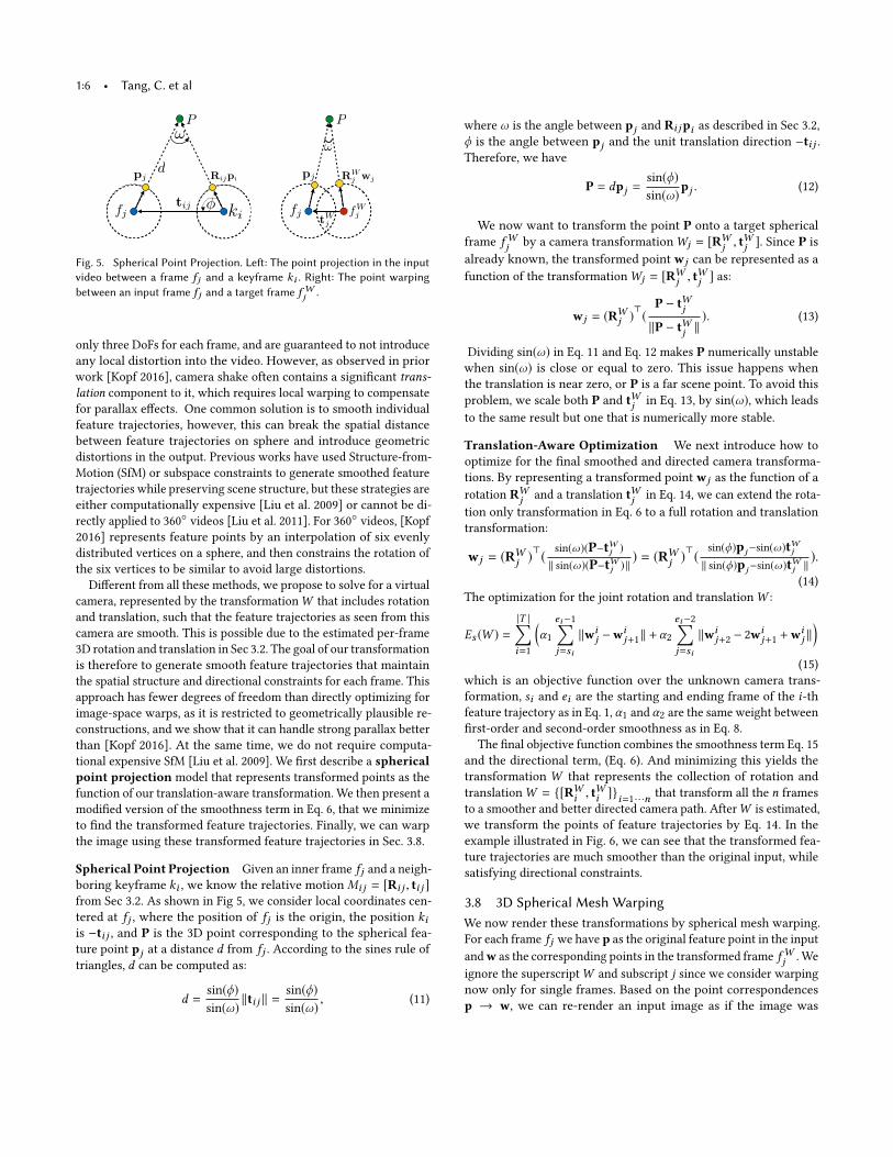
Fig. 5. Spherical Point Projection. Left: The point projection in the inputvideo between a frame fj and a keyframe ki . Right: The point warpingbetween an input frame fj and a target frame fWj .

only three DoFs for each frame, and are guaranteed to not introduceany local distortion into the video. However, as observed in priorwork [Kopf 2016], camera shake often contains a significant trans-lation component to it, which requires local warping to compensatefor parallax effects. One common solution is to smooth individualfeature trajectories, however, this can break the spatial distancebetween feature trajectories on sphere and introduce geometricdistortions in the output. Previous works have used Structure-from-Motion (SfM) or subspace constraints to generate smoothed featuretrajectories while preserving scene structure, but these strategies areeither computationally expensive [Liu et al. 2009] or cannot be di-rectly applied to 360◦ videos [Liu et al. 2011]. For 360◦ videos, [Kopf2016] represents feature points by an interpolation of six evenlydistributed vertices on a sphere, and then constrains the rotation ofthe six vertices to be similar to avoid large distortions.

Different from all these methods, we propose to solve for a virtualcamera, represented by the transformationW that includes rotationand translation, such that the feature trajectories as seen from thiscamera are smooth. This is possible due to the estimated per-frame3D rotation and translation in Sec 3.2. The goal of our transformationis therefore to generate smooth feature trajectories that maintainthe spatial structure and directional constraints for each frame. Thisapproach has fewer degrees of freedom than directly optimizing forimage-space warps, as it is restricted to geometrically plausible re-constructions, and we show that it can handle strong parallax betterthan [Kopf 2016]. At the same time, we do not require computa-tional expensive SfM [Liu et al. 2009]. We first describe a sphericalpoint projection model that represents transformed points as thefunction of our translation-aware transformation. We then present amodified version of the smoothness term in Eq. 6, that we minimizeto find the transformed feature trajectories. Finally, we can warpthe image using these transformed feature trajectories in Sec. 3.8.

Spherical Point Projection Given an inner frame fj and a neigh-boring keyframe ki , we know the relative motion Mi j = [Ri j , ti j ]from Sec 3.2. As shown in Fig 5, we consider local coordinates cen-tered at fj , where the position of fj is the origin, the position kiis −ti j , and P is the 3D point corresponding to the spherical fea-ture point pj at a distance d from fj . According to the sines rule oftriangles, d can be computed as:

d =sin(ϕ)sin(ω) ∥ti j ∥ =

sin(ϕ)sin(ω) , (11)

where ω is the angle between pj and Ri jpi as described in Sec 3.2,ϕ is the angle between pj and the unit translation direction −ti j .Therefore, we have

P = dpj =sin(ϕ)sin(ω)pj . (12)

We now want to transform the point P onto a target sphericalframe fWj by a camera transformationWj = [RWj , t

Wj ]. Since P is

already known, the transformed point wj can be represented as afunction of the transformationWj = [RWj , t

Wj ] as:

wj = (RWj )⊤(P − tWj∥P − tWj ∥

). (13)

Dividing sin(ω) in Eq. 11 and Eq. 12 makes P numerically unstablewhen sin(ω) is close or equal to zero. This issue happens whenthe translation is near zero, or P is a far scene point. To avoid thisproblem, we scale both P and tWj in Eq. 13, by sin(ω), which leadsto the same result but one that is numerically more stable.

Translation-Aware Optimization We next introduce how tooptimize for the final smoothed and directed camera transforma-tions. By representing a transformed point wj as the function of arotation RWj and a translation tWj in Eq. 14, we can extend the rota-tion only transformation in Eq. 6 to a full rotation and translationtransformation:

wj = (RWj )⊤( sin(ω)(P−tWj )∥ sin(ω)(P−tWj ) ∥ ) = (RWj )⊤(

sin(ϕ)pj−sin(ω)tWj∥ sin(ϕ)pj−sin(ω)tWj ∥ ).

(14)The optimization for the joint rotation and translationW :

Es (W ) =|T |∑i=1

(α1

ei−1∑j=si

∥wij −wi

j+1∥ + α2ei−2∑j=si

∥wij+2 − 2wi

j+1 +wij ∥)

(15)which is an objective function over the unknown camera trans-formation, si and ei are the starting and ending frame of the i-thfeature trajectory as in Eq. 1, α1 and α2 are the same weight betweenfirst-order and second-order smoothness as in Eq. 8.

The final objective function combines the smoothness term Eq. 15and the directional term, (Eq. 6). And minimizing this yields thetransformation W that represents the collection of rotation andtranslationW = {[RWi , t

Wi ]}i=1· · ·n that transform all the n frames

to a smoother and better directed camera path. AfterW is estimated,we transform the points of feature trajectories by Eq. 14. In theexample illustrated in Fig. 6, we can see that the transformed fea-ture trajectories are much smoother than the original input, whilesatisfying directional constraints.

3.8 3D Spherical Mesh WarpingWe now render these transformations by spherical mesh warping.For each frame fj we have p as the original feature point in the inputandw as the corresponding points in the transformed frame fWj . Weignore the superscriptW and subscript j since we consider warpingnow only for single frames. Based on the point correspondencesp → w, we can re-render an input image as if the image was

Joint Stabilization and Direction of 360◦ Videos • 1:7

Input

Warped

Fig. 6. Translation-Aware Optimization. The input trajectories (red) areshaky while the optimized trajectories (yellow) are smoother. At the sametime, the positive constraint (red ′+′ circle) is transformed to the front, whilethe negative constraint (blue ′−′ circle) is transformed to the back of thesphere.

Fig. 7. Spherical Mesh Warping. A set of feature correspondences (bluearrows) are used to drive a warp computed over the vertices of a sphere.The computed offset vectors at each vertex (red arrows) are used to warpthe vertices to the sphere on the right.

captured by a camera physically located on a well directed andsmooth 3D camera path without requiring full 3D reconstruction,which can be slow and unreliable [Liu et al. 2009]. As shown inFig 7, the general idea of our spherical mesh warping is to propagatethe point-wise correspondence to each mesh vertex in the imageand then warp the spherical image based on these vertices. Due toour 3D structure preservation, we can allow for a higher degree ofdeformation than prior work (we use a 20×10mesh), while avoidinggeometric distortion. Given the high mesh resolution, we found it tobe sufficient to use a regular grid defined on an equirectangular map,however different spherical tessellations could be used if desired.As described in Sec. 3.2, the translation induced motion can be

represented by feature dependent axis and angle. Sincewe’ve alreadyestimated the transformation rotation R and translation t, we knowthe axis as t×Rp for each feature point, and we get the angle ω inthe same way as in Sec. 3.2.We now have the rotation and translation between the input

and warped image and have estimated the angle ω (which is aparametrization of the point depth) for each feature in the frame.To propagate the warping motion from a set of feature points Fto a set of mesh vertices V in the corresponding spherical meshwarp, we apply the rotation R to all vertices and then solve for Eω ,the field of translation angles for all vertices by a 1D minimization

Fig. 8. A warped image and the interpolated angle ϕ shown for all pixels.This demonstrates how the warping angles have structure roughly similarto the inverse depth map but smooth, e.g., pixels closer to the camera onthe mountain have larger value than farther pixels under the same cameramotion.

parameterized only on the angle ω.

Eω =∑p∈F

∥ωp − b⊤p vp ∥22 +∑i, j ∈V

∥vi −vj ∥22 , (16)

where p belongs to the set of feature points, i and j ∈ V are neigh-boring vertices on sphere, vp are the angles for the four verticesthat cover the p-th feature point [Liu et al. 2009], and b⊤p is the cor-responding bilinear interpolation coefficients for the four vertices.The spatial smoothness term

∑ ∥vi −vj ∥22 guarantees that anglesare spatially smooth and avoids local distortion.

We solve Eq. 16 in a least squares sense, giving us the final outputposition for each vertex and use these vertex positions to render awarped sphere (Fig. 7). The 1D optimization defined in Eq. 16 hasthe advantage of being efficient to compute, while restricting oursolution to warps that are geometrically regularized. We bi-linearlyinterpolate the angle to all pixels and visualize it in Fig 8. Becausethe warping must only correct for residual motion, we observed,similar to prior work [Kopf 2016], that the warping function islargely smooth, and as such we have found this approach to berobust to input videos and parameter settings.

3.9 ImplementationOurmethod was implemented in C++.We solve Eq. 4 and Eq. 6 usingthe Levenberg-Marquardt algorithm in Ceres. We fixed parametersfor all the results shown here, although if desired we can easilycontrol the amount of smoothing by changing α1 and α2. We reportaverage running times for the different parts of our method in Tab. 1computed on a 2015 Macbook Pro laptop with 2.5GHz i7 CPU and16GB memory, on HD (1920 × 960) equirectangular video frames.

Section Average running timein ms/frame

Ingest and cube map conversion 5Feature tracking and keyframe selection (Sec. 3.1) 23Relative motion estimation (Eq. 4) 10Re-cinematography computation (Eq. 6) 1Full deformable warping (Eq. 16) 10Rendering in OpenGL 6

Total 55

Table 1. Running times for different parts of our method, computed on1920 × 960 video frames.

1:8 • Tang, C. et al

Tilt Z

Pan X

Fig. 9. Representative slices of the energy surface formed by Eq. 4, with blueshowing areas of lower energy. Here we show 2D slices of the original 6Derror space. This visualization indicates that the surface is largely smooth,which yields a robust and efficient optimization, despite the nonlinear energyterms.

4 RESULTS AND EVALUATION

4.1 Motion Estimation EvaluationWe first compare our motion estimation to the commonly used 5-point algorithm [Nister 2004]. As opposed to the 5-point algorithmwhich estimates an essential matrix, we directly solve for R and tusing non-linear least squares. We solve this minimization usingLevenberg-Marquardt optimization [Agarwal et al. 2017] with man-ually derived analytic derivatives which we show in the AppendixA. We empirically found this to converge by 10 iterations, takingroughly 20ms to estimate the motion for a pair of cameras withabout 3000 feature correspondences. Surprisingly, the optimizationconverges to a reasonable solution even when initialized with anidentity rotation matrix and a random unit translation vector. Tounderstand why, we visualize the error space by uniform sampling(two slices of which are shown in Figure 9), which shows that theenergy function is close to convex, making it efficient to solve ro-bustly. We also found that our motion estimation works well evenin cases with pure rotation, which is most likely due to the fact thatour method uses all feature points available in a 360◦ image, whichhelps to disambiguate rotation and translation motion. Compared tothe 5-point algorithm [Nister 2004], where epipolar constraint areenforced exactly (Eq. 2 equals to zero) within each 5-point group andthe solution is selected as the one with maximum inliers, our methodseeks for a solution with a minimum energy over all points, whichbenefits from a greater number of inliers, improving the accuracyof the motion estimation and mesh-based image warping.

We next evaluate the motion estimation quality in the presence ofnoise in the feature correspondences. A qualitative visualization offeature trajectories after stabilization using our method in place ofthe 5-point algorithm is shown in Fig. 11, with additional examplesin Sec. 4. Quantitative evaluation on real world data is challengingdue to the difficulty of collecting ground truth data for 3D poseestimation. We therefore employ the same validation techniqueused by prior motion estimation works [Kneip and Lynen 2013;Kneip et al. 2012; Nister 2004]. The approach is to use synthetic data,where the first camera is fixed at the origin with identity rotationand a second camera chosen at a random position at most τ unitsfrom the first with a relative rotation generated from random Eulerangles bounded to κ◦ . We then create a uniformly distributed 3Dpoint cloud with fixed maximum distance to the origin γ . Featurecorrespondences can then be computed by projecting the 3D points

0 0.2 0.4 0.6 0.80

0.5

1

Noise Added (deg)

Rotatio

nError(deg) Ours

R only5-point

0 0.2 0.4 0.6 0.80

0.5

1

Noise Added (deg)

TranslationError(deg)

Ours5-point

50 100 150 200 250 300 3500

0.5

1

1.5

FoV(deg)

Rotatio

nError(deg) Ours

5-point

Fig. 10. Validation of our proposed method on synthetic data. Top: Arotation-only model R (green) performs significantly worse than our fullapproach that models both R and 3D translation direction t (red), whichoutperforms the commonly-used 5-point algorithm (blue) in the presence ofincreasing noise. Middle: We observe a similar difference when comparingour recovered 3D translation direction to the 5-point algorithm. Bottom:When comparing the result quality at different FoV settings, we can see thatour direct estimation has consistently less error.

into the two spherical cameras with added noise. Finally, the relativemotion of the cameras are computed from this data and comparedto the known relative camera motion.For our experiments we use τ = 2, κ = 30◦ , γ = 8. We fix the

outlier percentage to 10% and solve for the relative poses 1000 timesat each noise level, recording the final average accuracy. As shownin Fig 10 our direct motion estimation is more accurate than the5-point algorithm for 360◦ video, and is more robust to increasingnoise levels due to the fact that it can consider a larger number ofbackground tracks. Estimating both rotation and translation alsoenables us to derive the 3D spherical warping proposed in Sec. 3.7.We also found the approach to be particularly robust to the field ofview (FoV) parameter for traditional video, which allowed us to use

Joint Stabilization and Direction of 360◦ Videos • 1:9

rotation only 5-point Ours

Fig. 11. Visualization of feature tracks after running our full method usingthe 5-point algorithm for estimating 3D rotation and translation (left) vsusing our proposed approach (right), showing that our result is smoother.Please see the supplemental video for a comparison.

0% 20% 40% 60% 80% 100%

Percentage of Meaurements

0.0001

0.001

0.01

0.1

1st-

ord

er

Sm

ooth

ness V

alu

e

Direct Estimation

Five-Point Algorithm

Rotation Only

First-order Smoothness

0% 20% 40% 60% 80% 100%

Percentage of Measurements

0.0001

0.001

0.01

0.1

2nd-o

rder

Sm

ooth

ness V

alu

e

Direct Estimation(Ours)

Five-point Algorithm

Rotation Only

Second-order Smoothness

Fig. 12. Quantitative comparison of first-order and second-order smooth-ness by different motion estimation methods. The curves show the cumula-tive distribution function of (a) first-order and (b) second-order smoothnesscosts for the feature trajectories stabilized by different motion estimationalgorithms. The y-axis represents the value of the first and second-ordersmoothness, and x-axis represents the percentage of the values larger thana corresponding y value.

a rough estimate of 120◦ horizontal FoV for all wide-angle videos,with the vertical FoV dependent on the aspect ratio.

In addition to the quantitative evaluation of ourmotion estimationin Sec. 3.2, we also show the smoothness of final results achievedby different motion estimation strategies. Similar to [Kopf 2016],we collect all feature trajectories and evaluate the value of first-order and second-order smoothness terms in Eq. 15. Fig. 12 showsthe cumulative distribution functions (CDFs) for these quantitiesby different motion estimation methods. We can see that featuretrajectories optimized by our translation-aware transformation aresmoother than 5-point algorithm, and that, as also noted in [Kopf2016] that rotation only model can not stabilize the video sufficiently.

4.2 Qualitative EvaluationIn this section, we perform ablation studies and compare alternativesfor each component of our method. For evaluation, we collected 12360◦ and 8 wide angle videos from YouTube, as well as 3 360◦ videosfrom the Pano2Vid dataset [Su et al. 2016]. The resolution rangesfrom 1920 × 960 to 3840 × 2160, for 360◦ videos, and 1280 × 720 to3840 × 2160 for wide angle videos, with unknown FoVs. We thentrim long videos such that the final duration ranges from 30-60seconds, which is long enough for viewers to fully explore the videoand much longer than prior datasets used for narrow FOV video

stabilization [Liu et al. 2013]. In Fig.14, we compare smoothnessnorms by visualizing the path of a scene point across frames. Pleasesee the supplemental video for reference.We present all video results in the supplemental material in

equirectangular format, which we encourage to be viewed on aVR headset if possible. If this is not possible, we provide a link to adesktop viewer where the videos can be explored by mouse as wellas a normal FoV video that presents select results.

Direction w/o Stabilization. Some recent works [Hu et al. 2017;Su and Grauman 2017; Su et al. 2016] focus on converting sphericalvideos to traditional narrow FoV videos. These works re-direct thevideo, but do not consider the camera motion in the original videos,assuming that the input is captured by static or smooth cameras.This assumption does not hold for many consumer videos capturedby hand-held cameras with shaky movement. As shown in Fig. 15,feature trajectories in the output of Pano2Vid are as shaky as theinput, while our result not only focus on the important content butachieves this with a smooth camera path.

Stabilization w/o Direction. Using our method we can alsogenerate stabilized-only results, and we provide some examples ofthis in the supplemental material. In general, videos that are entirelystabilized are hard to watch, as camera motion and objects of interestcan drift away from true north, causing viewers to get lost. Thiscan be seen in Fig. 18 (c,d), where when viewed with stabilizationbut without direction (b), the opposing kendo player moves aroundthe camera quickly, and many viewers loose track of the players,requiring some time for their gaze to catch up to the action. However,in the directed version (c), the opposing player is kept in the center,which makes viewing much easier. It is also possible to reintroducea smoothed version of the original viewing direction back into thevideo [Kopf 2016], however this is not sufficient in many cases, asthe original camera direction may often times not be ideal as shownin Fig. 16, and also can be seen in Fig. 18 (a,b).

Finally, as observed in our user study, and collaborated by otherperceptual studies [Sitzmann et al. 2018], many viewers tend towatch 360◦ content passively. We can see that the average viewingdirection is highly centered in the true north direction, independentof the video content. Therefore, it is crucial to direct interestingevents to this region.

Two-stage vs Joint Optimization. One question is whether it isnecessary to optimize the direction and smoothness jointly, or if sat-isfactory results could be obtained by stabilizing the inputs first andthen directing the output of stabilization. Some recent works [Huet al. 2017] uses the later strategy to generate 2D hyperlapse from 3Dspherical videos. We compare the two-stage optimization with ourjoint approach by first stabilizing the video ignoring the directionconstraint in Eq. 6, then we adjust the direction of the stabilizedresult by smooth interpolation of the positive direction constraints.As shown in Fig. 17, our approach creates smoother camera pathsoverall, as direction constraints may be inconsistent across time,and being able to jointly solve for both gives us more flexibility tochoose between multiple valid stable paths. This is especially truewith automatically generated constraints such as forward motion or

1:10 • Tang, C. et al

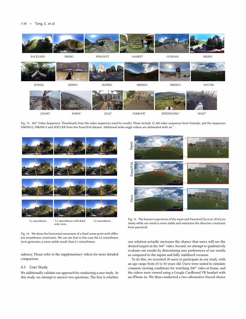
BACKYARD BIKING WINGSUIT MARKET GUNDAM HIKING

JUNGLE KENDO SLIDING HIKING2 HIKING3 SOCCER

CRANE∗ HAWK∗ LEGO∗ PARKOUR∗ SPEEDFLYING∗ WOLF∗

Fig. 13. 360◦ Video Sequences. Thumbnails from the video sequences used for results. These include 12 360 video sequences from Youtube, and the sequencesHIKING2, HIKING3 and SOCCER from the Pano2Vid dataset. Additional wide-angle videos are delineated with an ∗.

+

+

+

+

L1 smoothness

+

+

+

+

L1 smoothness with thirdorder term

+

+

+

+

L2 smoothness

Fig. 14. We show the horizontal movement of a fixed scene point with differ-ent smoothness constraints. We can see that in this case the L2 smoothnessterm generates a more stable result than L1 smoothness.

saliency. Please refer to the supplementary videos for more detailedcomparison.

4.3 User StudyWe additionally validate our approach by conducting a user study. Inthis study, we attempt to answer two questions. The first is whether

Inpu

tPano

2Vid

Ours

Fig. 15. The feature trajectories of the input and Pano2vid [Su et al. 2016] areshaky while our result is more stable and maintains the direction constraintfrom pano2vid.

our solution actually increases the chance that users will see thedesired targets in the 360◦ video. Second, we attempt to qualitativelyevaluate our results by determining user preferences of our resultsas compared to the inputs and fully stabilized versions.

To do this, we recruited 20 users to participate in our study, withan age range from 25 to 50 years old. Users were seated to simulatecommon viewing conditions for watching 360◦ video at home, andthe videos were viewed using a Google Cardboard VR headset withan iPhone 6s. We then conducted a two-alternative forced choice

Joint Stabilization and Direction of 360◦ Videos • 1:11Inpu

tDire

cted

Frame 0 Frame 200

Fig. 16. In the input video (top) the camera is mounted on a toy gun, whichis pointed down at the ground frequently . Using manual editing constraintswe can keep the video pointed ahead even when the gun is lowered, makingit much easier to watch.

+

+

+

Joint Optimization

+

+

+

Two-stage optimization

Fig. 17. A two-stage optimization can not guarantee the direction in theoutput is consistent since the direction constraint is generated for eachedited frame independently. So it is necessary to optimize with directionconstraints and smoothness constraints jointly to regularize the directionconstraint.

(2AFC) preference experiment, where viewers were presented withtwo versions of a video and after viewing both sequentially wereasked which they preferred. In addition, the gaze directions of eachviewer was recorded, to measure the overlap with the positive con-straint regions. The study included 6 videos, with an average lengthof 30 seconds. For each video, we compare the following versions:a) the original video, b) the stabilized only video, c) the directedand stabilized video via two-stage optimization and d) our directedand stabilized video via joint optimization. Comparisons are madeas pairwise choices, yielding 6 different pairwise comparisons per

Original Video Ours Stabilized

Mean distance (deg) 57.89 25.87 76.69Percent seen (%) 34.79 56.18 13.23

Table 2. Measured distance of participants’ gaze directions to the positivedirectional constraints (lower is better). We also show the percent of positiveconstraints likely seen, which corresponds to the fraction of constraintsthat were within 30◦ of a viewer’s gaze (higher is better).

video. Within each pair, video positions are randomized, and theorder of the 6×6=36 pairs is drawn randomly. Viewers were notgiven any specific viewing instructions besides simply exploringthe videos as they like.

To validate whether our method can be used to improve the view-ing experience by directing the camera towards important events,we compute two quantitative measures using the recorded viewingtracks. First, we measure the mean distance of all users to all positiveconstraints in the videos. Second, we compute what percentage ofviewers gaze was within 30◦ of the positive constraints. We cansee the results in Table 2, indicating that adding direction to thecamera significantly increased the chance that viewers will witnessthe events that the editor chooses to highlight. Figure 18 showsan example frame where the viewers have missed an importantevent in the undirected version. This is an important step to val-idate, given that the main goal of our approach is to increase thechance of seeing positively marked events. This is mostly due to theinherent preference for forward-facing viewing, and the problemwith getting lost when camera motion is not smooth. Please see thesupplemental material for a visualization of viewing direction ofparticipants.In the second experiment, we perform a qualitative test, where

users were asked for each pair, “which video did you prefer towatch?”. The results of this study are shown in Fig. 19. We useone-way analysis of variance (ANOVA) [?] to validate the statisticalsignificance of our results. To analyze the multiple preference testin a single ANOVA pass, we count the times that a specific versionwas selected as the preferred video, and use this as a score. Aftercollecting scores for all four different versions on all videos, werun one-way ANOVA to evaluate the statistics significance of thedifferences between different models. We find that the p-value ofthe ANOVA is 7.269 × 10−14, indicating that the conclusions of oursubjective evaluation are reasonable. As shown in Fig. 19, whencompared with the input, a vast majority of users preferred ourdirected and stabilized version to both the input and stabilizedfootage. When compared within the directed and stabilized version,the joint optimization approaches is slightly preferred over the two-stage optimization, indicating that the joint optimization has found agood balance between stability and direction, although this result isless statistically significant. We also conduct a comparison betweenthe stabilized version and the input, and found a slight preferenceof the stabilized version.We note that we conducted a relatively long term user study,

lasting 36 minutes for each viewer. To avoid viewers exceeding the

1:12 • Tang, C. et al

(a) Input (a) Directed (c) Stabilized (d) Directed

Fig. 18. Gaze directions from our user study visualized as a heatmap over the video frames. In (a), a large portion of viewers will miss seeing the robot fromthe front, as they remain looking around the direction of motion. In (b), the camera rotates quickly, moving the important action out of view. It takes sometime for users to find the kendo player again after this, whereas in the directed version, they can watch the whole scene without getting lost.

Scor

es

0.0

1.0

2.0

3.0Joint Optimization Two-Stage Optimization Stabilization Only Input

Pref

eren

ce

0%25%50%75%

100%125%

Pref

eren

ce

0%25%50%75%

100%125%

Pref

eren

ce

0%25%50%75%

100%125%

Pref

eren

ce

0%25%50%75%

100%125%

Pref

eren

ce

0%25%50%75%

100%125%

Pref

eren

ce

0%25%50%75%

100%125%

(a) (b) (c) (d) (e) (f) (g)

1

Fig. 19. Percentage of obtained votes from the user study, showing a slight preference for (a) joint direction and stabilization v.s. two-stage direction andstabilization, and strong preferences for (b) joint direction and stabilization v.s. stabilization only, (c) stabilization only v.s. input, (d) two-stage direction andstabilization v.s. stabilization only, and (e) two-stage direction and stabilization v.s. input. We also show a slight preference of (f) stabilization only v.s. input,and (g) the mean scores for each version.

maximum time that they were comfortable viewing 360°video, wesplit the 36 comparison pairs into 3 groups and let the viewers watchone group each time with rests in between. Longer experimentswould be needed to measure differences in viewing comfort overextended viewing sessions.

4.4 LimitationsOur method directs and stabilizes 360◦ or wide-angle videos basedon estimated 3D camera motion and directional constraints. Whilethis approach works well in many cases, it has some limitations.For one, we found that when videos were captured using multi-camera setups with imprecise temporal synchronization, the 3Dscene assumptions in Sec. 3.2 are no longer valid, and our methodis unable to compensate the shakiness in the input video.

Second, the joint direction and stabilization optimization in Sec. 3.2assumes that the input direction satisfies the cinematography rules.When the input direction constraint violates cinematographic rules,our joint optimization can not correct the direction constraint bysmoothness. We can see examples of this when viewing constraintsare derived for example from automatic saliency computations inthe supplemental material. Additionally, when foreground objects,especially those with coherent motion tracks, occupy the majorityof the viewing sphere, our optimization is unable to identify onlythe correct background tracks. Please see the supplemental videofor examples of these cases.

5 CONCLUSION AND FUTURE WORKIn conclusion, we have presented an approach for joint stabilizationand direction of 360◦ video. 360◦ video is particularly well suitedfor this task, as all views are present at capture time, allowing fullcontrol over viewing direction in post. In our work, we addressmodifying only the look-at direction, however this is just one smallpart of computational cinematography for 360◦ video, and thereare many interesting areas for follow up work. For example, wedo not experiment with changing focal length (zoom), as current360◦ cameras do not have suitable resolution for close-up shots.Recent work [Serrano et al. 2017] has studied how people react tocuts in 360◦ viewing, especially when important content regions areinconsistent across the cut. We validate our approach with a similarexperiment, in that we look at the percentage of fixation pointsof viewers inside regions of interest over short videos. However,our study is complementary, and shows how direction affects theviewing experience. These findings suggest our method could beused in conjunction with observations from Serrano et al. [2017]to automatically direct content to be consistent over cuts. Finally,we believe that virtual cinema experiences with wide angle footageis a good way to bridge the gap between the wide availability of360◦ viewing devices and the limited library of content. To thisend, our approach can be used with common wide angle first per-son cameras, as well as the recently introduced family of 180◦ VRcameras.

Joint Stabilization and Direction of 360◦ Videos • 1:13

REFERENCESSameer Agarwal, Keir Mierle, and Others. 2017. Ceres Solver. https://code.google.com/

p/ceres-solver/. (2017).Robert Anderson, David Gallup, Jonathan T. Barron, Janne Kontkanen, Noah Snavely,

Carlos Hernández, Sameer Agarwal, and Steven M. Seitz. 2016. Jump: Virtual RealityVideo. ACM Trans. Graph. 35, 6 (2016), 198:1–198:13.

Chris Buehler, Michael Bosse, and Leonard McMillan. 2001. Non-Metric Image-BasedRendering for Video Stabilization. In IEEE Conference on Computer Vision and PatternRecognition. 609–614.

Bing-Yu Chen, Ken-Yi Lee, Wei-Ting Huang, and Jong-Shan Lin. 2008. CapturingIntention-based Full-Frame Video Stabilization. Computer Graphics Forum 27, 7(2008), 1805–1814.

Y. Dai, H. Li, and L. Kneip. 2016. Rolling Shutter Camera Relative Pose: General-ized Epipolar Geometry. In 2016 IEEE Conference on Computer Vision and PatternRecognition (CVPR). 4132–4140. https://doi.org/10.1109/CVPR.2016.448

Vineet Gandhi, Remi Ronfard, and Michael Gleicher. 2014. Multi-clip video editingfrom a single viewpoint. In Proceedings of the 11th European Conference on VisualMedia Production. ACM, 9.

Michael L Gleicher and Feng Liu. 2008. Re-cinematography: Improving the cameraworkof casual video. ACM Transactions on Multimedia Computing, Communications, andApplications (TOMM) 5, 1 (2008), 2.

Amit Goldstein and Raanan Fattal. 2012. Video Stabilization Using Epipolar Geometry.ACM Trans. Graph. 31, 5 (2012), 126:1–126:10.

Jeremy J. Gray. 1980. Olinde Rodrigues’ paper of 1840 on transformation groups. Archivefor History of Exact Sciences 21, 4 (1980), 375–385. https://doi.org/10.1007/BF00595376

Matthias Grundmann, Vivek Kwatra, and Irfan Essa. 2011. Auto-directed video sta-bilization with robust L1 optimal camera paths. In Computer Vision and PatternRecognition (CVPR), 2011 IEEE Conference on. IEEE, 225–232.

R. I. Hartley and A. Zisserman. 2004. Multiple View Geometry in Computer Vision(second ed.). Cambridge University Press, ISBN: 0521540518.

Hou-Ning Hu, Yen-Chen Lin, Ming-Yu Liu, Hsien-Tzu Cheng, Yung-Ju Chang, andMin Sun. 2017. Deep 360 Pilot: Learning a Deep Agent for Piloting through 360ÂřSports Video. In Proceedings of the IEEE Conference on Computer Vision and PatternRecognition (CVPR).

Eakta Jain, Yaser Sheikh, Ariel Shamir, and Jessica Hodgins. 2015. Gaze-Driven VideoRe-Editing. ACM Trans. Graph. 34, 2 (2015), 21:1–21:12.

Jason Jerald. 2016. The VR Book: Human-Centered Design for Virtual Reality. Associationfor Computing Machinery and Morgan & Claypool.

L. Kneip and S. Lynen. 2013. Direct Optimization of Frame-to-Frame Rotation. In 2013IEEE International Conference on Computer Vision. 2352–2359. https://doi.org/10.1109/ICCV.2013.292

Laurent Kneip, Roland Siegwart, and Marc Pollefeys. 2012. Finding the exact rotationbetween two images independently of the translation. In Proc. of ECCV.

Johannes Kopf. 2016. 360Âř video stabilization. ACM Transactions on Graphics (TOG)35, 6 (2016), 195.

Johannes Kopf, Michael F Cohen, and Richard Szeliski. 2014. First-person hyper-lapsevideos. ACM Transactions on Graphics (TOG) 33, 4 (2014), 78.

Jungjin Lee, Bumki Kim, Kyehyun Kim, Younghui Kim, and Junyong Noh. 2016. Rich360:Optimized Spherical Representation from Structured Panoramic Camera Arrays.ACM Trans. Graph. 35, 4 (2016), 63:1–63:11.

Ken-Yi Lee, Yung-Yu Chuang, Bing-Yu Chen, and Ming Ouhyoung. 2009. Video stabiliza-tion using robust feature trajectories. In IEEE International Conference on ComputerVision. IEEE, 1397–1404.

Hongdong Li and Richard Hartley. 2006. Five-point motion estimation made easy. In18th International Conference on Pattern Recognition (ICPR’06), Vol. 1. IEEE, 630–633.

Feng Liu, Michael Gleicher, Hailin Jin, and Aseem Agarwala. 2009. Content-preservingwarps for 3D video stabilization. ACM Transactions on Graphics (TOG) 28, 3 (2009),44.

Feng Liu, Michael Gleicher, Jue Wang, Hailin Jin, and Aseem Agarwala. 2011. Subspacevideo stabilization. ACM Transactions on Graphics (TOG) 30, 1 (2011), 4.

Shuaicheng Liu, Lu Yuan, Ping Tan, and Jian Sun. 2013. Bundled camera paths for videostabilization. ACM Transactions on Graphics (TOG) 32, 4 (2013), 78.

Yasuyuki Matsushita, Eyal Ofek, Weina Ge, Xiaoou Tang, and Heung-Yeung Shum.2006. Full-Frame Video Stabilization with Motion Inpainting. IEEE Trans. PatternAnal. Mach. Intell. 28, 7 (2006), 1150–1163.

D. Nister. 2004. An efficient solution to the five-point relative pose problem. IEEETransactions on Pattern Analysis and Machine Intelligence 26, 6 (June 2004), 756–770.https://doi.org/10.1109/TPAMI.2004.17

Ana Serrano, Vincent Sitzmann, Jaime Ruiz-Borau, Gordon Wetzstein, Diego Gutierrez,and Belen Masia. 2017. Movie editing and cognitive event segmentation in virtualreality video. ACM Transactions on Graphics (TOG) 36, 4 (2017), 47.

Jianbo Shi and Carlo Tomasi. 1994. Good features to track. In IEEE Computer SocietyConference on Computer Vision and Pattern Recognition. 593–600.

V. Sitzmann, A. Serrano, A. Pavel, M. Agrawala, D. Gutierrez, B. Masia, and G. Wet-zstein. 2018. Saliency in VR: How Do People Explore Virtual Environments? IEEETransactions on Visualization and Computer Graphics 24, 4 (April 2018), 1633–1642.

https://doi.org/10.1109/TVCG.2018.2793599H. Stewenius, D. Nister, F. Kahl, and F. Schaffalitzky. 2005. A minimal solution for

relative pose with unknown focal length. In 2005 IEEE Computer Society Conferenceon Computer Vision and Pattern Recognition (CVPR’05), Vol. 2. 789–794 vol. 2. https://doi.org/10.1109/CVPR.2005.36

Hans Strasburger, Ingo Rentschler, and Martin Jüttner. 2011. Peripheral vision andpattern recognition: A review. Journal of vision 11, 5 (2011), 13–13.

Y. Su and K. Grauman. 2017. Making 360Âř Video Watchable in 2D: Learning Videogra-phy for Click Free Viewing. In 2017 IEEE Conference on Computer Vision and PatternRecognition (CVPR). 1368–1376. https://doi.org/10.1109/CVPR.2017.150

Yu-Chuan Su, Dinesh Jayaraman, and Kristen Grauman. 2016. Pano2Vid: AutomaticCinematography forWatching 360◦ Videos. InAsian Conference on Computer Vision.

Qi Sun, Li-Yi Wei, and Arie Kaufman. 2016. Mapping virtual and physical reality. ACMTransactions on Graphics (TOG) 35, 4 (2016), 64.

Bill Triggs, Philip F. McLauchlan, Richard I. Hartley, and Andrew W. Fitzgibbon. 2000.Bundle Adjustment — A Modern Synthesis. Springer Berlin Heidelberg, Berlin, Hei-delberg, 298–372. https://doi.org/10.1007/3-540-44480-7_21

Yu-Shuen Wang, Hongbo Fu, Olga Sorkine, Tong-Yee Lee, and Hans-Peter Seidel. 2009.Motion-aware temporal coherence for video resizing. ACM Transactions on Graphics(TOG) 28, 5 (2009), 127.

A DERIVATIVES OF MOTION ESTIMATIONIn this appendix, we give the analytic derivatives of our motionestimation. For the convenience of representation, we denote t×Rpin Eq. 4 as n and multiply the angleω to the rotation axis r asw. Wefirst give ∂E

∂n ,∂n∂w and ∂n

∂t , and then ∂E∂w and ∂E

∂t can be calculatedusing chain rule.

∂E∂n is derived as:

∂E

∂n=

q⊤√1 −

(q⊤n∥n∥

)2 ( I∥n∥ − nn⊤

∥n∥3), (17)

where I is a 3 × 3 identity matrix.∂n∂w and ∂n

∂t are:∂n∂w= t×(Rp)×, (18)

∂n∂t= (Rp)×. (19)

By chain rule we can finally get ∂E∂w and ∂E

∂t as ∂E∂w =

∂E∂n

∂n∂w

and ∂E∂t =

∂E∂n

∂n∂t .