jonesch05

7/17/2019 jonesch05

http://slidepdf.com/reader/full/jonesch05 1/19

5THE LEAP SECOND

International Earth Rotation Service

It may seem strange to devote a whole chapter to leap seconds, but

the story of how extra seconds are occasionally introduced into UTC

is a long and complex one. We’ll begin with an organisation called the

International Earth Rotation Service (IERS), whose sole job is to monitor

the rotation of the Earth and its orientation in space.

The IERS came into being on 1 January 1988. It took over the astro-

nomical functions of the BIH, whose responsibility for atomic time was

transferred to BIPM at the same time. IERS also took over the former

International Polar Motion Service, which was itself descended from the

International Latitude Service which started continuous monitoring of

polar motion in 1899.

IERS has many responsibilities apart from its duties in timekeep-

ing. First, it maintains the International Terrestrial Reference Frame,

which defines the precise locations of several hundred reference points

on the surface of the Earth to within a centimetre or so. This has many

applications in geology and geophysics. Secondly, IERS maintains the

International Celestial Reference Frame, which is a positioning system

widely used by astronomers and based on the precise positions of morethan 500 distant galaxies. The two frames are connected by continuous

monitoring of the rotation of the Earth.

Five quantities are routinely measured and between them they com-

pletely specify how the Earth is oriented in space. Four concern the

direction of the rotation axis: two of them specify the position of the

pole on the ground in comparison with a standard reference pole and the

other two specify the direction the pole is pointing in space. The fifth

quantity, and the most useful for timekeeping, is the type of Universal

Time known as UT1.

95

7/17/2019 jonesch05


96 THE LEAP SECOND

In Chapter 3 we saw that, since the 1950s, Universal Time has been

classified into UT0, UT1 and UT2. If a single observatory measures

UT from astronomical observations that time is UT0. With observations

from several observatories it is possible to correct for polar wobble and

the resulting UT is called UT1. UT1 is essentially a measure of the

rotational orientation of the Earth in space—the angle it has rotated

through. It is the time that is of direct interest to navigators who use

the Sun and stars, though it has to be said that there are not many of

those these days.

A third type of UT—known as UT2—is derived from UT1 by ap-

plying a standard formula which corrects approximately for the seasonal

fluctuations in the rotation rate. As a smoothly running time scale UT2

was important in the 1950s and 1960s but since the redefinition of UTC

in 1972 it no longer features much in timekeeping.

Between them, BIPM and IERS have to ensure that UTC stays atall times within 0.9 seconds of UT1. If it appears that UTC is likely to

go beyond that limit then IERS instructs BIPM to insert a leap second.

This chapter is concerned with how IERS monitors the rotation of the

Earth to obtain UT1, and how it decides when a leap second is required.

How UT1 is measured

All methods rely on determining the orientation of the Earth with re-

spect to external objects such as galaxies, stars, the Moon and artificial

satellites.

Traditional methodsUntil the 1980s measurement of Universal Time relied on measuring the

time at which the rotating Earth carried a known star across the meridian.

What was being measured was really sidereal time (see Chapter 1) which

was then corrected to give Universal Time, or strictly UT0. By gathering

observations from a network of stations several values of UT0 could be

combined to give UT1.

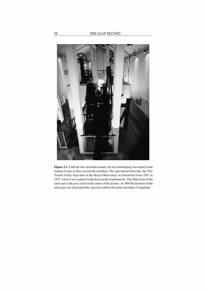
The simplest method is based on a specialised telescope called a

transit circle, first used by Danish astronomer Ole Romer in 1689 (Figure

5.1). It is a refracting telescope mounted so that it can sweep precisely

7/17/2019 jonesch05


How UT1 is measured 97

along the meridian from north to south but not away from it. The method

relies on knowing the precise position on the sky of a number of standard

stars. Let us suppose we use the bright star Capella. From astronomical

tables we can find that on 1 January 2000 Capella will cross the meridian

at 05:16:42 local sidereal time, which we can convert to UT0 using

standard formulae. So we point the transit circle at the meridian ahead of

Capella and wait for it to cross. The instant it crosses the line we know

UT0 and can set our clock accordingly. Using automated equipment it

is possible to measure UT to within a few milliseconds with a transit

circle.

A more sophisticated device is the photographic zenith tube (PZT),

a fixed telescope that points straight upwards. Designed in 1909, the

PZT was, until very recently, the instrument of choice for precise moni-

toring of the Earth’s rotation. An image of a small patch of sky directly

overhead is reflected from a pool of mercury (defining a precise hori-zontal surface) and four images of the stars are recorded on a moving

photographic plate along with the clock times of the exposures. Careful

measurement of the plate gives a very accurate transit time. Because it is

precisely aligned on the zenith, the PZT can measure the latitude of the

observatory as well as UT, and so monitor polar motion. PZTs were used

by the US Naval Observatory to relate UT to ET as part of the calibration

of the atomic second in the 1950s.

The newest device for measuring Earth rotation by the stars is the

Danjon astrolabe, invented by the same Andre Danjon who first pro-

posed the use of Ephemeris Time in the 1920s. First used in 1951, the

astrolabe determines the instant at which a star reaches an altitude above

the horizon of precisely 30 degrees. It can look in any direction, so canmeasure many more stars than either a transit circle or a PZT.

Ultimately, each of these techniques is limited by the accuracy with

which the instrument can be aligned and the positions of stars listed in

catalogues. What really made optical methods obsolete was the much

greater precision that became possible from other techniques in the

1970s and 1980s. Indeed, a few modern transit telescopes are still in

use, but they are now used the opposite way: knowing the precise time

of transit from an atomic clock, astronomers can get accurate positions

of the stars.

7/17/2019 jonesch05


98 THE LEAP SECOND

Figure 5.1. Until the late twentieth century all our timekeeping was based on the

timing of stars as they crossed the meridian. This specialised telescope, the Airy

Transit Circle, kept time at the Royal Observatory in Greenwich from 1851 to

1927, whenit was replaced with more modern instruments. The object lens of the

telescope is the grey circle in the centre of the picture. In 1884 the location of the

telescope was internationally agreed to define the prime meridian of longitude.

7/17/2019 jonesch05



VLBI

The most powerful of the modern methods of monitoring the Earth’srotation is called very long baseline interferometry, or VLBI. Devel-

oped from techniques pioneered in radio astronomy in the 1950s, VLBI

links together many widely spaced radio telescopes, often thousands

of kilometres apart, so that they act in concert to “synthesise” a much

bigger telescope equal in size to the widest spacing between the ob-

servatories. We will not go into the detail here, save to say that each

observatory agrees to observe the same astronomical object at the same

time and records the signals on a high-speed tape deck. The tapes are

then played back together and the signals combined to create an image

of the object in fabulous detail. VLBI observations now produce radio

images which are far more detailed than those from optical telescopes.

A consequence of this is that the positions of some of the most distant

objects in the universe—the fantastically powerful galaxies known as

quasars—are known far more accurately than any star. It then becomes

possible to use this precision to determine UT1.

To use VLBI for Earth rotation studies, the times at which

radiowaves from a known quasar arrive at each of the telescopes

are extracted from the tapes. The differences in arrival times can then be

used to calculate the orientation of the Earth with respect to the quasar.

Because the position of the quasar is accurately known, the orientation

of the telescope array, and hence the Earth, can be calculated to less than

one-thousandth of a second of arc.

VLBI observations are routinely carried out on about 500 quasars.

In 1997 more than a quarter of a million observations were made from

35 telescopes. Among these are regular observations carried out bynetworks in the US, Europe and Japan.

VLBI measures the rotation of the Earth in comparison to the most

distant objects in the universe. Unless the universe as a whole is rotating

in some sense, then this technique determines the absolute orientation of

the Earth in space, both the position of the pole and UT1.

Lunar laser ranging

When Apollo 11 landed on the Moon in July 1969, one of the pack-

ages placed on the Sea of Tranquillity by astronauts Neil Armstrong and

7/17/2019 jonesch05


100 THE LEAP SECOND

Edwin Aldrin was a flat box containing an array of 100 light reflectors.

Similar in principle to the reflectors on the backs of cars, the array was

designed to reflect pulses of laser light from Earth straight back to where

they came from. The idea was to measure the precise distance from the

Earth to the Moon.

Light travels through space at almost exactly 300 000 kilometres per

second. The Moon’s distance varies, but on average it is about 384 000

kilometres from Earth. A pulse of light will take about 1.3 seconds to get

from the Earth to the Moon. The round trip, after being reflected from the

Apollo 11 array, will be about 2.6 seconds. If the time between sending

the pulse and seeing the reflected flash can be measured accurately, then

the distance to the Moon can be calculated with equal accuracy.

Following the Apollo 11 mission, a similar array was left in the Fra

Mauro uplands by Apollo 14 in 1971 (Figure 5.2) and a bigger one in

the Apennine foothills by Apollo 15 in the same year. Arrays were alsotaken to the Moon on the Soviet automated rovers Lunokhod 1 (Sea of

Rains 1970) and Lunokhod 2 (Sea of Serenity 1973), although the former

is no longer operating.

Lunar laser ranging presents formidable challenges. Normal

sources of light are not strong enough to do the job and spread out too

much: even a pulse from a powerful laser spreads to a circle about 7

kilometres in diameter at the distance of the Moon. A tiny fraction of

that light—about a billionth—falls on the array and is reflected back.

The returning flash from the Moon also spreads out, and forms a circle

20 kilometres in diameter on the Earth. A collecting telescope picks up

at most only two-billionths of that light. Add to that the other losses,

and it turns out that out of every 10

21

photons sent towards the Moononly one will be detected back at the Earth.

Small wonder that very few observatories have the dedication to

continue lunar laser ranging. The main centres since 1969 have been the

McDonald Observatory in Texas, the Haleakala satellite station on Maui

in Hawaii (now discontinued), and a purpose-built station at Grasse in

the south of France. Interest does seem to be picking up again, with a

new station being constructed at Matera in southern Italy.

The accuracy of lunar ranging has improved steadily since the

1970s, and it is now possible to measure the distance between the ground

7/17/2019 jonesch05



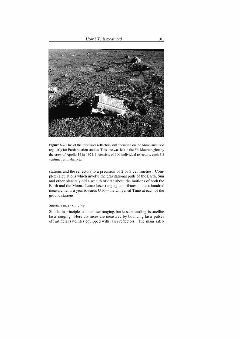
Figure 5.2. One of the four laser reflectors still operating on the Moon and used

regularly for Earth rotation studies. This one was left in the Fra Mauro region by

the crew of Apollo 14 in 1971. It consists of 100 individual reflectors, each 3.8

centimetres in diameter.

stations and the reflectors to a precision of 2 or 3 centimetres. Com-

plex calculations which involve the gravitational pulls of the Earth, Sunand other planets yield a wealth of data about the motions of both the

Earth and the Moon. Lunar laser ranging contributes about a hundred

measurements a year towards UT0—the Universal Time at each of the

ground stations.

Satellite laser ranging

Similar in principle to lunar laser ranging, but less demanding, is satellite

laser ranging. Here distances are measured by bouncing laser pulses

off artificial satellites equipped with laser reflectors. The main satel-

7/17/2019 jonesch05


102 THE LEAP SECOND

lites in use are the two Laser Geodynamics Satellites, known as Lageos,

launched in 1976 and 1992. The satellites are purpose-made for laser

ranging, consisting of a brass core within a 60-centimetre spherical alu-

minium shell covered in 426 reflectors. Each has a mass of more than

400 kilograms.

They orbit at a height of 5900 kilometres, which is high enough not

to be seriously affected by the remaining air in the outer reaches of the

atmosphere, and are visible from all parts of the world. More than 30

ground stations track the satellites, measuring their distances to better

than 2 centimetres.

The satellites orbit around the Earth’s centre of mass. Meanwhile,

the Earth rotates beneath them, and by careful measurements of the

positions of the satellites the rotation of the Earth can be monitored.

About 9000 passes are tracked each year. Satellite laser ranging is best

for daily measurements of polar motion, though it is also used for short-term measurements of UT1.

GPS

The US military Global Positioning System (GPS) has revolutionised

timekeeping in several ways. In Chapter 4 we saw how its “constel-

lation” of 24 satellites is used to transfer time from the world’s time-

keeping centres to BIPM and we shall come back to that in the next

chapter. But it is also used to monitor the rotation of the Earth. At least

five satellites are visible at all times from any point in the world, and

sometimes as many as eight or ten in certain locations. By processing

time signals from them it is possible to determine the position of the

receiver on the Earth to high accuracy. By continual monitoring from a

network of 30 ground stations, IERS can track the rotation of the Earth.

Using GPS, IERS measures UT1 to within 60 microseconds in the short

term, and provides daily measurements of polar wobble.

DORIS

The newest technique for monitoring Earth rotation is known as DORIS:

Doppler Orbitography and Radiopositioning Integrated on Satellite.

DORIS relies on a worldwide network of about 50 radio beacons whose

7/17/2019 jonesch05


How the Earth’s rotation has varied 103

signals can be received by a suitably equipped satellite. So far only

the French SPOT and US Topex satellites have DORIS equipment, but

others will follow shortly. The satellite measures the frequency of the

radiowaves received simultaneously from up to two beacons within

sight. The waves are Doppler shifted by the motion of the satellite,

and so an on-board computer can determine the speed of the satellite

with respect to the beacons, and from there the precise orbit can be

calculated. DORIS was originally intended to provide accurate heights

for ocean survey satellites, but is now being used for other geophysical

projects. Information about the rotation of the Earth is deduced in a

similar way to GPS and laser ranging.

How the Earth’s rotation has varied

In this section we will look at how the rotation of the Earth has varied

over the years as revealed by the changing length of the day. Figure 5.3

shows the average length of the day for each year since 1700, compared

with a standard day of 86 400 SI seconds, that is, exactly 24 hours. Up

until the 1960s these measurements derive exclusively from astronomi-

cal observations of star transits. The most recent ones use the methods

we have just described. Because these are yearly averages they do not

show the faster variations which we will come to shortly. But they do

reveal the medium- and long-term changes over the past three centuries.

It is striking that there seems to be no pattern in these variations. If

the Earth is steadily slowing due to tidal drag from the Moon, then itdoes not show up here. The length of the day seems to vary without any

discernible pattern. The most we can say is that changes are occurring

on the scale of decades which can alter the length of the day by up to 4

milliseconds.

Throughout the eighteenth and nineteenth centuries the length of

the day kept close to 86 400 seconds—except towards the end of this

period—and this is as expected: the ET second was defined in terms of

the average mean solar second during this period and the SI (atomic)

second was chosen to match the ET second as closely as possible.

7/17/2019 jonesch05


104 THE LEAP SECOND

–4.0

–2.0

0.0

2.0

4.0

1700 1750 1800 1850 1900 1950 2000

L e n g t h o f d a y i n e x c e s s

o f

2 4 h o u r s ( m i l l i s e c o n d s )

Figure 5.3. Historical records allow astronomers to reconstruct how the length

of the mean solar day has changed over the past three centuries. A sudden but

short-lived lengthening of the day in the late 1950s corresponds to the slowing

down recorded in Figure 3.1.

Why the rotation is not constant

Long-term changes

In Chapter 1 we saw how Edmond Halley struggled to explain discrep-

ancies between the position of the Moon in his time and many centuries

earlier. It later turned out that these differences were caused by the

tidal drag of the Moon on the Earth, causing the Earth to gradually lose

rotational energy and speed. The world was turning faster in the past and

the day was shorter.

Current best estimates are that tidal drag is lengthening the day by

2.3 milliseconds per century and has been doing so for at least 2700years. But historical research by Richard Stephenson at Durham Uni-

versity and Leslie Morrison at the Royal Greenwich Observatory shows

that tidal drag by itself is not enough to account for all the changes over

that period. By studying timings of eclipses from as long ago as 700 BC,

they found that at least two other effects seem to be at work as well.

One of these “non-tidal” effects tends to shorten the day by an aver-

age of 0.6 milliseconds per century. This process is a bit of a mystery, but

a plausible explanation is that the shape of the Earth has been changing

since the end of the last ice-age some 10 000 years ago. As the ice sheet

7/17/2019 jonesch05


Why the rotation is not constant 105

retreated towards the poles, the newly exposed land expanded upwards

as the overlying weight was removed. The effect of this “post-glacial

rebound” is that the Earth is becoming more spherical. Its equatorial

bulge is being pulled in, and as it does so its rotation tends to speed up.

A second effect is even more mysterious. The Earth appears to

be speeding up and slowing down over a period of about 1500 years,

varying the length of the day by about 4 milliseconds either way. Among

the ideas put forward to explain this are movements in the core of the

Earth (see the next section) and changes in sea level.

Taken together, these three effects cause the day currently to

lengthen by an average of 1.7 milliseconds per century. But from the

figure we see little evidence of this slowing. The reason is that the

diagram is dominated by much larger fluctuations that occur over much

shorter intervals. In the long run, tidal drag is slowing the Earth but

as far as present-day timekeeping is concerned its effects are almostentirely negligible.

Random variations

The most obvious variations occur on scales of decades, and these are the

fluctuations that cause the most trouble to timekeepers. If you look back

to Figure 3.1, which shows how the length of the UT second was chang-

ing between 1955 and 1958 while NPL and USNO were calibrating the

atomic second, you can see that the apparently straight line corresponds

to a short and wholly untypical section of this diagram where the Earth

was slowing unusually quickly. Shortly afterwards it started speeding up

again before embarking on another slowing that lasted to the mid-1970s.

In the 1990s the Earth was speeding up again and in the middle of 1999the length of the day briefly touched 86 400 seconds exactly.

Data from before 1800 are rather uncertain, but what are we to make

of the deep dip in the record in the mid-1800s and the even larger peak

in the early 1900s?

It now seems that the origins of these fluctuations lie deep within

the Earth, at the boundary between the core and its mantle (Figure 5.4).

The Earth’s core is made of iron and nickel, and at the temperatures and

pressures prevailing at these depths the outer part of the core is molten.

The liquid metal can flow, and indeed circulating flows in the core

7/17/2019 jonesch05


106 THE LEAP SECOND

Figure 5.4. Slow and irregular changes in the length of the day are believed to

be caused by movements in the liquid outer core below the Earth’s mantle.

give rise to the Earth’s magnetic field. By studying small changes in the

magnetic field, geophysicists can work out what is happening in the core.

It turns out that these motions are very slow, less than a millimetre per

second, but they are irregular, and the idea is that their magnetic fields

will pull and push on the overlying solid mantle, tending to speed it up or

slow it down. There may even be upside-down “mountains” on the lower

surface of the mantle which the molten metal pushes against as it flows

past. At present there does not seem to be any way in which we can pre-

dict these flows and the consequent fluctuations in the Earth’s rotation.

Seasonal variations

As we saw in Chapter 1, the seasonal fluctuations in the length of theday were discovered in the 1930s, and were really the final straw for

timekeeping based on the mean solar day. Figure 5.3 contains yearly

averages so these variations do not show up. But the next diagram

(Figure 5.5) shows the day-to-day changes in the length of the day for

the last three years. We are looking here at the very end of the curve in

Figure 5.3, where the day is steadily shortening.

The shortening is apparent in this graph also, but now we see clear

evidence of a regular change through the year. The size of this seasonal

variation is comparable to the longer-term changes, but it is much faster.

7/17/2019 jonesch05


Why the rotation is not constant 107

–0.5

0.0

0.5

1.0

1.5

2.0

2.5

3.0

3.5

Jan 1997 Jan1998 Jan 1999 Jan 2000

L e n g t h o f d a y i n e x c e s s o f

2 4 h o u r s ( m i l l i s e c o n d s )

Figure 5.5. Daily measurements of the length of the day are plotted for the

years 1997 to 1999. A gradual speeding up is discernible, as are the seasonal

variations through the year. The rapid fluctuations are caused by lunar and solar

tides distorting the shape of the Earth. The length of the day fell below 24 hours

on two occasions, in June and July 1999.

The variation is double-peaked, with the Earth turning slowest in spring

and autumn, and speeding up sharply in mid-summer. A lesser speeding

up is apparent around New Year, but this is not so clear.

It is now certain that these variations are caused by the

changing atmospheric circulation through the year. As weather patterns

alter, the directions and strengths of the winds also change. Winds

blowing against mountains are quite capable of changing the Earth’srotation by a measurable amount. Fluctuations on the scale of 30–60

days are also apparent and they too are thought to be due to winds.

Measurements of changes in the angular momentum of the atmosphere

match the changes in length of day very closely.

Ocean currents probably play a small part as well, though they are

much more constant than air movements. An interesting event occurred

early in 1983 when the day suddenly lengthened by about a millisecond

for a few weeks. This coincided with the El Nino phenomenon, where

ocean currents in the eastern Pacific reverse direction, accompanied by

7/17/2019 jonesch05


108 THE LEAP SECOND

unusual patterns of atmospheric pressure.

Figure 5.5 also shows much faster regular variations with periods

of two and four weeks. These are caused by tides raised in the Earth by

the Sun and the Moon. As the tides distort the shape of the Earth, the

period of rotation changes too.

The leap second

So far we have been discussing how the length of the day varies. The

fluctuations seem rather small, and have never differed more than 4

milliseconds from 24 hours over the past 300 years. A millisecond is

indeed a very short time. A point on the Earth’s equator would turn

about half a metre in a millisecond, and we might wonder whether the

effects on timekeeping are equally small. In fact, they are considerable.

Let us suppose the day is a constant 1 millisecond longer than 24

hours. And let us also suppose we check the time kept by the rotating

Earth—UT1—every day against an atomic clock ticking SI seconds.

After 1 day UT1 will lag by 1 millisecond. The next day it will lag

by 2 milliseconds. After a year it will lag by 365 milliseconds, and the

difference is becoming noticeable. After 10 years the Earth clock will be

lagging 3.65 seconds behind the atomic clock.

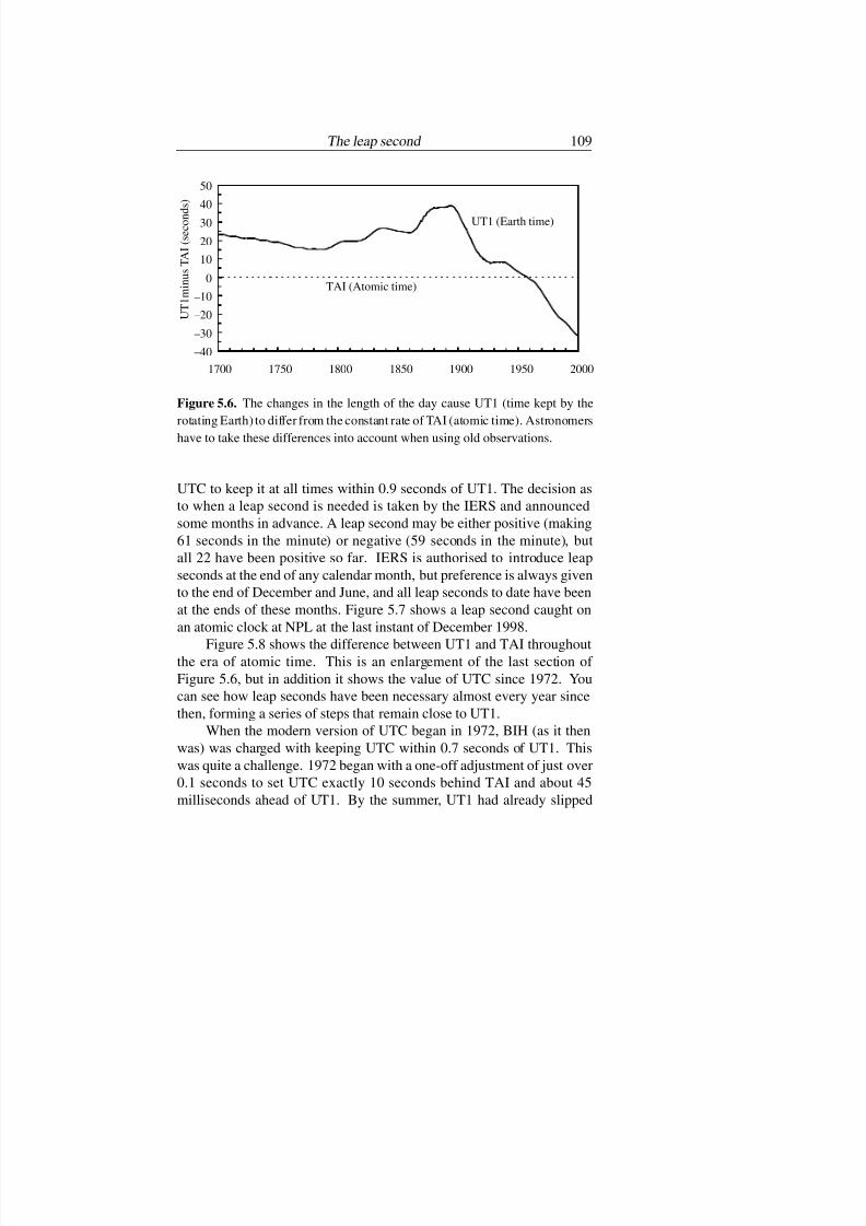
Figure 5.6 shows the cumulative difference between UT1 and TAI

recorded over the past 300 years. Of course, atomic time has only existed

since 1955 (and only called TAI in retrospect) but it is possible to track

the difference by using Ephemeris Time for the earlier dates.

Here in one diagram is the problem with atomic timekeeping. A

perfectly accurate clock, ticking SI seconds and set to TAI in 1958,would have been running at least 15 seconds behind UT1 during the

eighteenth century and 20–40 seconds behind during the nineteenth. Yet

in the twentieth century it would appear to have speeded up from 35

seconds behind in 1900 to more than 30 seconds ahead at the end of the

1990s. No wonder astronomers have abandoned timekeeping based on

the Earth’s rotation! We see also why TAI alone is not a good time scale

for precision timekeeping and why it was so dif ficult for timekeepers to

reconcile TAI with UT1 in the 1960s.

The solution, effective since 1972, is to insert a leap second into

7/17/2019 jonesch05


The leap second 109

–40

–30

–20

–10

0

10

20

30

40

50

1700 1750 1800 1850 1900 1950 2000

U T 1 m i n u s T A I ( s e c o n d s )

UT1 (Earth time)

TAI (Atomic time)

Figure 5.6. The changes in the length of the day cause UT1 (time kept by the

rotating Earth) to differ from the constant rate of TAI (atomic time). Astronomers

have to take these differences into account when using old observations.

UTC to keep it at all times within 0.9 seconds of UT1. The decision as

to when a leap second is needed is taken by the IERS and announced

some months in advance. A leap second may be either positive (making

61 seconds in the minute) or negative (59 seconds in the minute), but

all 22 have been positive so far. IERS is authorised to introduce leap

seconds at the end of any calendar month, but preference is always given

to the end of December and June, and all leap seconds to date have been

at the ends of these months. Figure 5.7 shows a leap second caught on

an atomic clock at NPL at the last instant of December 1998.

Figure 5.8 shows the difference between UT1 and TAI throughoutthe era of atomic time. This is an enlargement of the last section of

Figure 5.6, but in addition it shows the value of UTC since 1972. You

can see how leap seconds have been necessary almost every year since

then, forming a series of steps that remain close to UT1.

When the modern version of UTC began in 1972, BIH (as it then

was) was charged with keeping UTC within 0.7 seconds of UT1. This

was quite a challenge. 1972 began with a one-off adjustment of just over

0.1 seconds to set UTC exactly 10 seconds behind TAI and about 45

milliseconds ahead of UT1. By the summer, UT1 had already slipped

7/17/2019 jonesch05


110 THE LEAP SECOND

Figure 5.7. The last minute of 1998 had 61 seconds. The leap second was caught

by this atomic clock at NPL.

–35

–30

–25

–20

–15

–10

–5

0

5

1955 1960 1965 1970 1975 1980 1985 1990 1995 2000

T i m e s

c a l e m i n u s T A I ( s e c o n d s ) TAI (Atomic time)

UT1 (Earth time)

UTC (Clock time)

Figure 5.8. This enlargement of the last part of Figure 5.6 shows how, since

1972, UTC has been kept within 0.9 seconds of UT1 by the insertion of

occasional leap seconds.

7/17/2019 jonesch05


The leap second 111

more than 0.6 seconds behind UTC and the first leap second was intro-

duced at the end of June. At the end of the year, UT1 was starting to fall

behind again and a second leap second was thought necessary, but that

brought UT1 a full 0.81 seconds ahead of UTC which was technically

out of bounds. The limit was relaxed from 0.7 to 0.9 seconds in 1974,

and since then UTC has never departed more than 0.78 seconds from

UT1, and that was in June 1994.

The IERS publishes its continuous monitoring of the Earth’s rota-

tion in its Bulletin A, a twice-weekly report that is as comprehensible

to the casual reader as BIPM’s Circular T. If you want to see one it can

be downloaded from the IERS website (see Appendix). Each Bulletin

A contains preliminary results for the previous few days; namely the

position of the pole and the difference between UT1 and UTC, calculated

from the methods described earlier in this chapter. At present, daily

values of UT1–UTC and the length of the day can be measured to withina few microseconds. Bulletin A also contains forecasts of UT1–UTC

for up to a year ahead, though the uncertainty mounts rapidly the longer

the prediction. At the time of writing, in the spring of 2000, Bulletin A

reveals that the divergence between UT1 and UTC has slowed, and it is

clear that UTC will still be comfortably ahead of UT1 by the end of 2000

and no leap second will be needed before the beginning of 2001, if then.

Every month IERS issues two months’ worth of final results in Bul-

letin B, which also lists measurements derived from each of the observ-

ing techniques that have been used in that period. When IERS decides a

leap second will be needed, it issues the announcement some months in

advance in its Bulletin C.

How many leap seconds do we really need?

It is often said that leap seconds are necessary because the rotation of

the Earth is slowing. A casual reading of this chapter and other litera-

ture about leap seconds may indeed lead to the notion that the Earth is

slowing down and leap seconds are needed to give it time to catch up.

This is not the case. For most of the 1990s the Earth has been speeding

up (from year to year anyway) and is now at its fastest for 60 years. Yet

we have had 22 leap seconds in the past 27 years. So why, really, do we

need leap seconds?

7/17/2019 jonesch05


112 THE LEAP SECOND

You may remember at the beginning of Chapter 4 we pointed out the

problem of building identical clocks. No matter how carefully they are

built, two clocks will always run at slightly different rates and so, in time,

their readings will diverge noticeably. The principal reason that UT1

diverges from TAI, and the reason we need leap seconds, is because they

have been running at different rates for several years—UT1 ticks more

slowly than TAI. The mean solar second of UT1 since 1955 has been

somewhat longer than the atomic SI second of TAI. This is unavoidable,

since the atomic second wascarefully chosen to correspond to the second

of Ephemeris Time, which was approximately the average length of the

mean solar second in the eighteenth and nineteenth centuries. It follows,

however, that UT1 and TAI would have diverged less if the SI second

had been defined differently.

Suppose the SI second, defined by the caesium transition, had been

chosen to be equal to the mean solar second on 1 January 1958, whenTAI was set equal to UT1. Instead of being defined as 9192 631 770

periods of the caesium transition it could have been defined as about

9192 631 937 periods, the length of the mean solar second in January

1958 (Figure 3.1). That is a tiny difference—less than two parts in 100

million—but how would our timekeeping have been affected?

Figure 5.9 shows the difference. By 1999 UT1 would have been

barely 8 seconds behind TAI instead of more than 31, and since 1972

we would have needed only six leap seconds instead of 22. And that

dramatic difference is caused merely by defining the second to agree

with UT rather than with ET. Unfortunately that option was no longer

available in 1958. By then the ET bandwagon was rolling and the CGPM

was already committed to an SI second based on it.We can do even better, with the benefit of hindsight this time, by

asking what length of second would have minimised the discrepancy

between TAI and UT1. That turns out to be 9192 631 997 caesium

periods. With the second defined that way, UT1 would always have been

within 2 seconds of TAI since 1955—sometimes ahead and sometimes

behind—and there would have been only three leap seconds since 1972,

two negative and one positive. And with the rates of TAI and UT1 much

closer, these leaps would have been genuine consequencesof the changes

in the length of the day.

7/17/2019 jonesch05


The leap second 113

–35

–30

–25

–20

–15

–10

–5

0

5

1955 1960 1965 1970 1975 1980 1985 1990 1995 2000

U T 1 m i n u s T A I ( s e c o n d s )

(a) SI second

(b) Mean solar second

in January 1958

(c) Optimum second since 1955

TAI

Figure 5.9. TAI was defined to be equal to UT1 in January 1958. Since then, the

two scales have diverged because the SI second (a) has been slightly longer than

the second of UT1. If the SI second had been set equal to the second of UT1

in 1958 (b), the divergence would have been less. With the benefit of hindsight,

we can even define an optimum second (c) that would have kept UT1 within 3

seconds of TAI since 1958. The frequent occurrence of leap seconds in UTC is

primarily due to the chosen length of the SI second, not changes in the rotation

of the Earth.

This is not the whole story of course. The apparent convenience

of maintaining TAI close to UT1 since 1955 is—

alas—

countered by thehavoc wreaked on the history of astronomy. From Figure 5.6 we see

that in 1700, for example, UT1 was 23 seconds ahead of TAI. With our

redefined 1958 second that would have changed to 123 seconds behind

TAI and with our optimum second it would have been 178 seconds

behind—almost three minutes. So on balance, it may be better to leave

time as it is.

jonesch05

Documents