jonny nilimaa - diva portal
TRANSCRIPT

Upgrading the Haparanda Bridge A case study
Jonny Nilimaa
Department of Civil, Environmental and Natural resources engineering
Luleå University of Technology
SE-97187 Luleå, Sweden


i
Preface
The case study presented in this report has been carried out at the
Division of Structural and Construction Engineering, Department of Civil, Environmental and Natural resources engineering, at Luleå
University of Technology, Sweden, during the summer of 2012. The
work has been financially supported by the Swedish Transport Administration, Trafikverket.
The work presented is a full scale strengthening of a concrete railway bridge located in Haparanda.
The author wants to acknowledge the Swedish Transport
Administration for their financial and scientifical support. The staff at Complab, LTU, is also acknowledged for their support and assistance
during the installation of monitoring system, as well as strengthening and monitoring of the bridge.
Luleå, November 2012
Jonny Nilimaa

ii

iii
Abstract
This report presents the design and results of the strengthening of a
double trough concrete railway bridge in Haparanda, Sweden. The objective was to find a strengthening solution, which provides a
sufficient shear capacity in the transversal direction for the bridge slab
when the allowed axle loads on the railway are increased from 25 to 30 ton.
Unbonded post-tensioning was chosen as the strengthening method and the design was performed according to the design criteria of
Eurocode. The results indicate increased interaction between the two
troughs, as well as an increased capacity. All reinforcement strains caused by a train with 21.5 ton axle loads were counteracted by the
compressive action obtained by eight prestressing bars, stressed with 430 kN/bar.
The main conclusion was that the load carrying capacity increased
significantly and the effect is probably higher than what is shown in the design calculations.

iv

v
Table of content
PREFACE ....................................................................................................................... I
ABSTRACT .................................................................................................................. III
1.INTRODUCTION ....................................................................................................... 1
1.1. BACKGROUND ..................................................................................................................... 1 1.2. STRENGTHENING ................................................................................................................. 2 1.3. THE HAPARANDA BRIDGE ................................................................................................... 3
2.METHOD ................................................................................................................... 5
2.1. BRIDGE GEOMETRY AND MATERIALS ................................................................................... 5 2.2. STRENGTHENING PROCEDURE ............................................................................................ 8 2.2.1. Drilling of holes ........................................................................................................ 8 2.2.2. Installation of prestressing system .................................................................................. 10 2.2.1. Post-tensioning ....................................................................................................... 11 2.2.2. Sealing ................................................................................................................. 13 2.3. MONITORING .................................................................................................................... 14 2.3.1. Strains.................................................................................................................. 14 2.3.1. Deflections ............................................................................................................. 15 2.3.1. Joint opening .......................................................................................................... 15 2.4. TEST PROGRAM ................................................................................................................. 18
3.STRENGTHENING DESIGN ...................................................................................... 21
3.1. SHEAR STRENGTHENING .................................................................................................... 21 3.1.1. Eurocode 2 ............................................................................................................ 22 3.2. FLEXURAL CAPACITY.......................................................................................................... 24 3.3. DESIGN OF DISTRIBUTION WEDGES .................................................................................... 25
4.RESULTS ................................................................................................................... 27
4.1. STRAINS ............................................................................................................................. 27 4.2. DEFLECTIONS ..................................................................................................................... 28 4.2.1. Deflections along transversal line .................................................................................. 28 4.2.1. Deflections along longitudinal line under main trough ........................................................ 28 4.2.1. Deflections along longitudinal line under secondary trough ................................................... 28 4.3. JOINT OPENING .................................................................................................................. 37
5.ANALYSIS ................................................................................................................. 39
5.1. STRAINS ............................................................................................................................. 39 5.2. DEFLECTIONS ..................................................................................................................... 40 5.3. JOINT OPENING .................................................................................................................. 40
6.DISCUSSION ............................................................................................................. 41
7.CONCLUSION ........................................................................................................... 45
8.FUTURE RESEARCH ................................................................................................. 47
9.REFERENCES ............................................................................................................ 49
APPENDIX A – DOCUMENTATION OF TEST PROCEDURE ...................................... 53
APPENDIX B – TEST RESULTS ................................................................................... 65
APPENDIX C – DESIGN CALCULATIONS ................................................................... 97

vi

1
1. Introduction
1.1. Background
About two thirds of the over 300,000 railway bridges in Europe are
more than 50 years old [1]. With time, the structures have been
exposed to various destructive stresses in form of e.g. chemical- and physical deterioration which might have affected the structural
performance. During these years, the application areas and bridge demands have probably also changed a number of times. Today the
traffic intensities, -loads and –velocities are much higher than they
were fifty years ago and prevailing design codes have also changed several times.
The concrete trough bridge is almost a standard type of bridge that was built in Sweden during the 1950’s. Until the year of 1950, the largest
axle loads had been kept at a maximum of 200 kN [2], but at this
point, two new load models with axle loads of 250 kN were introduced [3]. This was the highest axle loads in Sweden until the
1990’s when the mining industry required higher capacity and the
“iron ore line” increased the axle loads up to 300 kN [4]. Today, most railway lines in Sweden are still having 225 or 250 kN as the
maximum axle load, but new lines are designed for 330 to 400 kN.
In order to upgrade a concrete bridge, the design calculations are
currently following the directions of Eurocode 2 [5]. Previous design
calculations [6] have revealed the shear capacity in the transversal direction of trough slabs as a problem area, i.e. the capacity is
insufficient for 300 kN axle loads.

2
1.2. Strengthening
The technique of precision drilling long holes through a concrete or
rock structure may be used to introduce extra reinforcement in areas which otherwise are inaccessible. This technology has been tested
previously, e.g. in [7], but the method can be further developed using post-tensioning which is a classic way of preventing further cracking in
concrete or metallic structures.
In order to increase the shear- and flexural capacities in the transversal direction of a concrete slab, a prestressing force could be introduced.
The prestressing force can be obtained by installing an internal bonded or unbonded post-tensioning solution, consisting of prestressing bars or
tendons, transversally inserted through the slab. By choosing a low
vertical placement of the prestressing bar, the effect on flexural capacity increases, but existing reinforcement layers in the slab might aggravate
the choice of a low placement.
Laboratory tests [8] indicated that post-tensioning is an appropriate
method, but both Eurocode [5] and the Swedish design code [9] are
restrictive in estimating the strengthening effects.
One of the advantages of the post-tensioning method is the low
disturbance of existing traffic on the railway line during strengthening. All strengthening work is performed under the top-level of the bridge,
which is good for safety reasons, and the traffic can go on as planned
during the execution. The main advantages of choosing an unbonded strengthening solution is that the level of prestress can easily be
adjusted and single strands can be exchanged, if necessary. The risks of this strengthening method includes accidental cutting of the internal
reinforcement during drilling.
A small number of trough bridges have been strengthened previously by Luleå University of Technology [10 – 12], but the main focus has
been on increasing the flexural capacity either in the longitudinal or horizontal direction.

3
1.3. The Haparanda Bridge
The Haparanda Bridge is a concrete double trough bridge, with a span
of about 12.5 m. The geographical location of the bridge is Haparanda in northern Sweden, close to the border to Finland, see Fig. 1.1. A
two-line main road runs underneath the bridge, which was built in 1959 [13-19], and the bridge crosses the road with an angle of 73°.
The purpose of this case study is to investigate whether the method of
unbonded internal post-tensioning can be applied for upgrading the trough bridges from a maximum allowed axle load of 250 kN to 300
kN, or not. Strengthening effects in terms of steel strains and structural deformations are also investigated.
Figure 1.1 - Location of the Haparanda Bridge.
The strengthening method is transversal post-tensioning of the slab and
the strengthening design was derived through a three step assessment; 1) Initial assessment – site visit, documentation investigations and
simple calculations. 2) Intermediate assessment – further inspections,
material testing and detailed calculations. 3) Enhanced assessment – Laboratory testing, strengthening design and monitoring.

4
Prestressing does not only increase the shear capacity of the slab, the
flexural capacity in the horizontal direction is also affected and the strengthening design follows the directions of Eurocode. According to
the design calculations, the shear and flexural capacities are increased
by 25% and 13%, respectively.
The bridge was tested before and after strengthening, and the results
indicates that the additional steel strains caused by a train with axle loads of 215 kN is completely counteracted by the prestressing.
Maximum steel strains caused by the train is however small,
magnitudes of 20 µm/m, which implies on a higher original capacity of the bridge.

5
2. Method
A double trough bridge was strengthened by installing an unbonded
prestressing system in the structure. The prestressing system introduced a transversal force, compressing the bottom slab and increased the load
carrying capacity by decreasing the tensile stresses in the structure.
2.1. Bridge geometry and materials
The bridge is a reinforced concrete trough bridge with two separate
troughs, one for each railway track. A main road is running underneath
the bridge, where the superstructure has an angle of 73° to the supporting substructure, as seen in Figure 2.1. Internal transverse
reinforcement in the superstructure was cast in the same direction as the substructure, i.e. with an angle of 73° from the longitudinal line.
The free span of the bridge is 12537 mm and the total width of the
both troughs is 10510 mm, including top flanges. The height is 1200 mm and 1300 mm for external and internal girders, respectively. Slab
thickness is 400 mm. A side view of the bridge is shown in Figure 2.2 and Figure 2.3 gives a view of the cross section.

6
Figure 2.1 – Plan of the bridge in Haparanda. All measurements are given in mm.
Figure 2.2 – Side view of the Haparanda Bridge. All measurements are given in mm.

7
Transversal top and bottom reinforcement in the slab both have
diameters of 19 mm and other dimensions used are diameters of 12 mm and 25 mm. The steel quality was denoted KS40, with a
characteristic yield strength of 410 MPa and Youngs modulus of 200
GPa. No tests were however performed on the reinforcement from the actual structure. Concrete quality was tested on four concrete cylinder
cores and reported in [6]. Concrete compressive and tensile strengths were 23.2 MPa and 1.5 MPa, respectively. The characteristic material
properties are summarized in Table 2.1.
Figure 2.3 – Cross section of the Haparanda Bridge. All measurements are given in mm.
Eight prestressing threadbars, denoted Dywidag 26WR, with nominal
diameters of 26.5 mm were used to post-tension the trough bridge in
the transversal direction. The prestressing bars are hot-rolled, tempered from the rolling heat, stretched and annealed, with a circular cross
section. The bars are of prestressing steel Y1050H according to prEN 10138-4:2000, [21], and the characteristic values were provided by the
manufacturer as 1050 MPa and 205 GPa for the tensile strength and
Youngs modulus, respectively.

8
Table 2.1 – Characteristic material properties.
Diameter,
d
[mm]
Compressive
strength,
σc
[MPa]
Tensile
strength,
σt
[MPa]
Youngs
modulus, E
[GPa]
Concrete - 23.2 1.5 30
Reinforcement 19 410 410 200
Prestressing bars 26.5 1050 1050 205
2.2. Strengthening procedure
The concrete double trough bridge was strengthened with an unbonded post-tensioning system and the strengthening procedure was
divided into four strategic working steps;
1. Drilling of horizontal holes, transversally through the bottom
slab.
2. Installation of prestressing system.
3. Post-tensioning.
4. Sealing of the prestressing system.
The advantage of having an unbonded strengthening solution is that
individual bars can easily be replaced if they are accidentally damaged,
corroded or no longer needed, and the level of prestress can be adjusted later if required.
2.2.1. Drilling of holes
Eight horizontal holes were drilled transversally through the bottom
slab of the two troughs. Core drilling was the method used for this
application and the holes had diameters of 57 mm. The holes were drilled in the same direction as the transversal reinforcement, i.e. with
an angle of 73° versus the concrete surface. The reason for having transversal reinforcement in this direction is to align it with the
substructure and the reason for drilling the holes in the same direction
is to prohibit unwanted cutting of reinforcement while drilling.

9
The slab has a thickness of 400 mm and the holes were located in the
vertical mid-section, i.e. the centers of the holes were located 200 mm from the slabs bottom surface. The main reason to have the holes in
the mid-section instead of at lower position, which would give a
higher flexural capacity in the strengthening application, was to prevent cutting of the existing internal reinforcement.
A total number of eight holes with a lateral center-to-center distance of 1500 mm were drilled trough the structure. The lateral center-to-
center distance was estimated according to design directions in
Eurocode 2, section 8.10.3(5), in order to obtain full compressive action within the entire length of the slab. Geometry and denotation of
prestressing bars are shown in Fig 2.4.
Figure 2.4 – Plan view and denotation for prestressing bars. Bars are represented by the thicker lines. All measurements are given in mm.

10
2.2.2. Installation of prestressing system
The installation of the prestressing system can be divided into four consecutive sub-steps, carrying on after the drilling;
1. Installation of PE ducts.
2. Installation of prestressing bars.
3. Installation of load distributing wedges, see Fig. 2.5.
4. Installation of anchoring system.
Corrosion protection is an important part of the installation procedure
and the sustainability is strongly dependent on the measures for water protection.
Installation of PE ducts
The first step in the installation of the prestressing system was to insert
ducts into the drilled holes. The ducts can either be made of steel or
Polyethylene, PE, and the latter alternative was chosen for this project. The function of the duct is to provide a mechanical protection for the
heat shrinking sleeve, which surrounds the prestressing bar. The heat shrinking sleeve, in turn, provides a permanent corrosion protection
for the prestressing steel.
Installation of prestressing bars
After the ducts had been installed in the transversally drilled holes, the
prestressing bars penetrated the ducts. As stated earlier, the prestressing bars had a permanent corrosion protection in form of a heat shrinking
sleeve, covering the steel surface. The prestressing bars require being
longer than the drilled holes to make the anchoring and prestressing possible and the length is governed by the prestressing equipment and
anchoring design. The prestressing bars were installed in the center of the ducts and left unbonded.

11
Installation of load distributing wedges
The contact between the prestressing system and the concrete structure requires being perpendicular to ensure an effective stress transfer from
the prestressing bars to the concrete structure. Since the holes were
drilled with an angle of 73°, instead of 90°, a galvanized steel wedge was specially designed to obtain the required perpendicular stress
distribution. The wedges also functioned as load distributors, distributing the prestressing force over a larger concrete area and
preventing local concrete crushing or splitting behind the post-
tensioning anchors. All steel wedges were bonded to the concrete surface in order to keep them stable during installation and prevent
water leakage into the holes.
Installation of anchoring system
The anchoring system consisted of square galvanized steel anchor
plates, with dimensions of 140 mm x 165 mm x 35 mm, and anchor nuts with the length of 90 mm. The anchor nuts have the purpose of
anchoring the prestressing bars at a certain stress level and transferring the prestressing force from the bar to the structure. The anchor plates
are normally in direct contact to the concrete structure, distributing the
prestressing force from the anchor nuts directly to the concrete structure. But the bearing surface of the anchor plate must be
perpendicular to the prestressing bar, which is partly why load distributing wedges were used as a compensating layer and all anchor
plates were bonded to the load distributing plates in order to prevent
water leakage into the holes. The load distributing wedge and the anchoring system is shown in Fig. 2.5.
2.2.1. Post-tensioning
When the prestressing system had been installed, the post-tensioning
procedure started. The eight prestressing bars were post-tensioned with
a force of 430 kN per bar, resulting in a total force of 3.44 MN acting on the concrete slab. A hydraulic jack was used for the stressing part.
The hydraulic pressure corresponding to a prestressing force of 430 kN was first calibrated against a load cell.

12
Figure 2.5 – Load distributing wedge and anchoring system.
A steel frame was designed to ensure stressing of the bars. The steel frame had openings on the bottom side and the top side, and one of
the side walls had an opening for access to the anchor nut. The bottom side of the steel frame rested on the anchor plate, with the prestressing
bar running through the bottom and top openings, while the anchor
nut was inside of the frame.
The hydraulic jack was positioned on the prestressing bar, resting on
the top side of the steel frame. An extra nut was screwed on the end of the prestressing bar, which protruded the jack. With the extra nut as a
resistance at the stressing side of the slab and the anchor nut as a
resistance on the other side, the bridge could finally be post-tensioned. During stressing, the anchor nut on the stressing side of the slab was
continuously tightened.
After reaching the desired prestressing force and tightening the anchor
nut as much as possible, the pressure in the hydraulic jack was released
and the prestressing force could be transferred from the prestressing bar to the concrete structure. An instant strain relaxation of approximately
6% took place as the hydraulic stress was released and all bars were

13
overstressed in order to obtain 430 kN as the final prestressing force.
Finally the extra nut, hydraulic jack and steel frame could be removed. The prestressing setup is illustrated in Fig. 2.6.
Figure 2.6 – Prestressing setup including; steel frame, hydraulic
jack and an extra prestressing nut.
2.2.2. Sealing
The strengthening system contains mainly steel parts and if the
strengthening parts are left untreated, corrosion might corrupt the
strengthening effect. To obtain a sustainable strengthening system, it requires a valid corrosion protection solution. The corrosion
protection solution for this system was to seal the strengthening system after post-tensioning.
First, the prestressing bars had a permanent corrosion protection in
form of a heat shrinking sleave, surrounding the bars. Secondly, the sleeve was protected against mechanical impacts by the PE duct. The
connection between the steel wedge and the concrete structure, as well as between the steel wedge and the anchor plate was sealed by a
permanent water resistant compound (epoxy adhesive).
Finally, the anchor nuts and bar ends were sealed by a welding a retention cap to the anchor plate. All steel wedges, anchor plates and
retention caps were galvanized as a corrosion protecting measure. The retention cap is shown in Fig. 2.8.

14
Figure 2.8 – A complete post-tensioning system sealed with a retention cap.
2.3. Monitoring
Structural movements and displacements were monitored by linear
variable differential transformers (LVDTs) and crack opening displacement transformers (CODs). Steel strains were monitored by
strain gauges (SGs), welded to the reinforcement and prestressing bars.
2.3.1. Strains
Four strain gauges were welded onto the slabs internal transversal
bottom reinforcement (S1-S4) and four additional SGs were welded on prestressing bars P1 – P4 (S5-S8). The locations of reinforcement SGs
and prestressing SGs are shown in Fig. 2.9 and 2.10, respectively. S1
and S2 coincide with the longitudinal location of prestressing bar P1, while S3 and S4 coincide with the longitudinal location of prestressing
bar P4.

15
2.3.1. Deflections
A total number of 16 LVDTs (L1-L16) monitored the vertical displacements of the structure, six in a transversal line beneath
prestressing rod P4, as seen in Fig. 2.11, and the remaining 10 in two
longitudinal lines in the mid-section of the two bridge slabs, as seen in Fig 2.12.
2.3.1. Joint opening
The Haparanda Bridge consisted of two concrete troughs. The troughs
were most likely cast at two separate occasions and the distance
between the troughs at the connection joint was monitored by three CODs (C1-C3). The CODs measured the differential transversal
movement of the two troughs at the joint, as seen in Fig. 2.13.
Figure 2.9 – SGs on internal transversal bottom reinforcement. All measurements are given in mm.

16
Figure 2.10 – SGs on prestressing bars. All measurements are given in mm.
Figure 2.11 – LVDTs in transversal direction. All measurements are given in mm.

17
Figure 2.12 – LVDTs in longitudinal direction. All measurements are given in mm.
Figure 2.13 – CODs along the connection joint. All measurements are given in mm.

18
2.4. Test program
The test program for the Haparanda Bridge was divided into two test
occasions; one test prior to strengthening and one test after strengthening. Each test run included eight tests, two static and six
dynamic tests, with known velocities. The complete test program for the Haparanda Bridge is given in Table 2.2 and 2.3. There was a speed
limit of 20 km/h on the railway line over the bridge due to the nearby
railway depot, restricting the maximum test velocity to 20 km/h.
Table 2.2 – Test program for the unstrengthened bridge.
Test Track Direction Velocity [km/h]
St1:1 Main North 0
St2:1 Secondary North 0
Dy1:1 Main North 5
Dy2:1 Main South 5
Dy3:1 Main North 10
Dy4:1 Main South 10
Dy5:1 Main North 20
Dy6:1 Main South 20
Table 2.3 – Test program for the strengthened bridge.
Test Track Direction Velocity [km/h]
St1:2 Main North 0
St2:2 Secondary North 0
Dy1:2 Main North 5
Dy2:2 Main South 5
Dy3:2 Main North 10
Dy4:2 Main South 10
Dy5:2 Main North 20
Dy6:2 Main South 20

19
The load consisted of two coupled diesel locomotives, GC Td44, with
an axle load of 215 kN, see Fig. 2.14. The axle distance of the locomotives was such that a maximum of two axles were located on
top of the bridge slab during the tests. At the static tests, the
locomotives were placed with the two axles on an equal distance, on both sides of the midspan.
Figure 2.14 – The two locomotives used as loads on the Haparanda Bridge. North is located in the left direction.

20

21
3. Strengthening Design
3.1. Shear strengthening
The shear capacity was calculated according to the European design
code; Eurocode 2, [5].
The code is in some sense based on the addition principle, where the
total shear resistance, VR, of a member without shear reinforcement, is calculated as the sum of the shear strengths of concrete, VC, and the
prestressing,
PCR VVV (1)
The contribution from prestressing is however included in the
concrete resistance, as seen in Equation (4). If the member contains shear reinforcement, the concrete resistance will be replaced by the
shear resistance of the stirrups, as seen in Equation (2).
SR VV (2)
In order to provide a safe structure, the total shear resistance, VR, must
be greater than the shear forces, VE, resulting from all loads acting on the structure as shown in Equation (3).
ER VV (3)
Design calculations for the shear capacity of the slab, in the transversal
direction has previously been presented in [6], resulting in a lack of shear capacity of 24%. The critical section is located at the distance x =
2.998 m from the center of gravity of the free edge beam. The shear

22
capacity at this section is 150 kN/m and the shear force is 186 kN/m,
thus requireing a strengthening providing a minimum of 36 kN/m in shear capacity.
The strengthening method used to increase the capacity is internal
post-trensioning, which will introduce the term VP into the equation for the shear resistance, VR.
3.1.1. Eurocode 2
The general procedure for shear design of concrete structures is
presented in chapter 6.2 of Eurocode 2. The design value for the shear
resistance is given by the following equation;
dbσk)fρ(kCV wcpcklRd,cRd,c
1
31
100 (4)
with a minimum of;
dbσkVV wcpRd,c 1min (5)
As seen in Equation (4), the shear capacity of the prestressing is included in the shear resistance of the concrete. The contribution from
the prestress can be separated from the equation and expressed as;
dbσkV wcpRd,P 1 (6)
The values for k , 1k , Rd,cC and minV can be found in the National Annex
for each country, but the recommended values are;
0.2200
1 d
k (7)
15.01 k (8)
c
Rd,cC
18.0 (9)
21
23
min 035.0 ckfkV (10)

23
where;
c is the partial factor, which can be chosen as 1.2 or 1.5,
depending on the design situation,
020.db
Aρ
w
sll
(11)
slA is the area of the tensile reinforcement, which extends
dlbd beyond the section considered.
ckf is the characteristic compressive cylinder strength of
concrete at 28 days.
The stress, caused by prestressing is;
cd
c
Edcp f
A
Nσ 2.0 [MPa] (12)
where;
EdN is the axial force in the cross section due to loading or
prestressing.
cA is the area of the concrete cross section.
wb is the smallest width of the cross-section in the tensile
area.
d is the effective depth of a cross-section.
In order to increase the shear capacity of the Haparanda Bridge by 36
kN, a prestressing force of at least 260 kN/m is required.

24
3.2. Flexural capacity
The flexural capacity of the cross-section shown in Figure 3.1 below is
determined by defining the equilibrium equations.
Figure 3.1 – Forces acting on a prestressed cross section.
Assuming yielding in the tensile reinforcement, the horizontal
equilibrium equation will be;
0' SSC FPFF (13)
Equation (13) can be developed into the following expression;
0''8.0 SstSSScc AfPAEbxf (14)
The distance to the neutral layer, x, can be solved with the following
equation;
1
2
C
Cx
(15)
where
SstSSS
cc
AfPAEC
bfC
''
8.0
2
1
(16)
Through moment equilibrium around the concrete resultant force, we get;

25
04.0'4.02
4.0
MxdFx
hPxdF SS
(17)
where the moment can be solved as;
xdAExh
PxdAfM SSSSSst 4.0'''4.02
4.0
(18)
By introducing a prestressing force of 286 kN/m, the flexural capacity of the Haparanda Bridge will increase from 257 kNm/m to 295
kNm/m.
3.3. Design of distribution wedges
The contact between the prestressing system and the concrete trough
bridge requires being perpendicular to ensure an effective stress transfer
from the prestressing bars to the bridge. Since the holes were drilled with an angle of 73°, instead of 90°, a galvanized steel wedge was
specially designed to obtain the required perpendicularity. The wedges
also functioned as load distributors, distributing the prestressing force over a larger concrete area and preventing local concrete crushing or
splitting behind the post-tensioning anchors.
As a simplification Eurocode, section 8.10.3(5), states that the
prestressing force may be assumed to disperse at an angle of 2 , starting
at the end of the anchoring device. The value of is assumed to be;
7.333
2arctan .
The prestressing force is transferred from the bar, through the anchor plate and the distribution wedge, onto the concrete structure. The
external main girder of the trough bridge has a width of 857 mm and is
assumed to act as a load distribution device for the concrete slab. The force is dispersed over a distance of 571 mm by passing through the
girder and if the c/c distance for the prestressing bars is chosen as 1500 mm, the required width of the distribution wedge therefore becomes
mm 35857121500 .
A width of 382 mm was finally chosen for the distribution wedges, as seen in Fig. 3.2.

26
Figure 3.2 – Load distribution through the main girders. All measurements are given in mm.

27
4. Results
Selected test results are presented in this section, remaining results are
found in Appendix B. The denotation for the results are the type AaX:Y. The full test program, including denotation is given in Table
2.2 and 2.3, but a short summary is given below;
Aa – Letter that represents the load type. (St – Static loading, the train is standing still on the bridge. Dy – Dynamic
loading, the train is moving at a constant speed over the bridge)
X – Number that represents the test number. (1-2 for static
loads and 1-6 for dynamic loads)
Y – Number that reveals if the test is performed prior to
strengthening or after strengthening. (1 – Prior to strengthening. 2 – After strengthening)
4.1. Strains
The strain levels were calibrated prior to the testing of the unstrengthened bridge, meaning all strains caused by e.g. dead-loads,
ballast, etc. are not included in the strain results. Figs. 4.1 – 4.4 presents
the strain curves for the two static tests and Figs. 4.5 – 4.8 presents strains in S3 and S4 during dynamic loading. The only strains measured
in the tests prior to strengthening are the ones caused by the train loads. When the bridge was post-tensioned, the prestressing
compressed the reinforcement, causing a negative value for the strain
readings after strengthening. The reinforcement was compressed

28
differently at the four measuring locations and the strain curves are
therefore starting at different strain levels for the different strain gauges.
The strains in the prestressing bars during static loading of the main
trough are presented in Fig. 4.9 and the strain in prestressing bar P4
during dynamic loading is presented in Fig 4.10.
4.2. Deflections
4.2.1. Deflections along transversal line
The deflections were monitored along three separate lines as seen in Fig. 9 and 10. All LVDTs were calibrated prior to testing of the
unstrengthened bridge and the results from the static loading of the main trough are presented in Figs. 4.11 – 4.12. The prestressing bars
that were placed close to the neutral layer of the slab and the post-
tensioning did not have any influence on the deflections of the unloaded bridge, i.e. the deflection curves starts at 0 both before and
after strengthening. The deflection curves for dynamic loading showed almost similar behavior as for static loading and the magnitudes were
actually slightly lower for dynamic loading.
4.2.1. Deflections along longitudinal line under main trough
The Haparanda Bridge consisted of two troughs with a railway track on top of each trough. The main track was the track used as the
transportation track and the secondary track was only used for station
activity purposes, i.e. arranging and managing train sets during loading of the trains. The deflections along the longitudinal line under the
main trough are presented in Figs. 4.13 – 4.14.
4.2.1. Deflections along longitudinal line under
secondary trough
Deflections were monitored along two longitudinal lines; under the central line of the main and secondary troughs, respectively. The
deflections under the secondary trough are presented below. The deflections along the longitudinal line under the secondary trough are
presented in Figs. 4.15 – 4.16.

29
Figure 4.1 – Strains for Static loading of the main track before strengthening.
Figure 4.2 – Strains for Static loading of the main track after
strengthening
-40
-30
-20
-10
0
10
20
30
40
0 60 120 180 240 300 360 420 480
Str
ain
[µm
/m
]
Time [s]
Strains (St1:1)
S1 S2
S3 S4
-40
-30
-20
-10
0
10
20
30
40
0 60 120 180 240
Str
ain
[µm
/m
]
Time [s]
Strains (St1:2)
S1 S2
S3 S4

30
Figure 4.3 – Strains for the static loading of the secondary track before strengthening.
Figure 4.4 – Strains for the static loading of the secondary track after strengthening.
-40
-30
-20
-10
0
10
20
30
40
0 60 120 180 240 300
Str
ain
[µm
/m
]
Time [s]
Strains (St2:1)
S1 S2
S3 S4
-40
-30
-20
-10
0
10
20
30
40
0 60 120 180 240 300
Str
ain
[µm
/m
]
Time [s]
Strains (St2:2)
S1 S2
S3 S4

31
Figure 4.5 – Strain in S3 for the dynamic loading of the main track with a constant train speed of 20 km/h in southerly direction before strengthening.
Figure 4.6 – Strain in S3 for the dynamic loading of the main track with a constant train speed of 20 km/h in southerly direction after
strengthening.
-40
-30
-20
-10
0
10
20
30
40
0 5 10 15 20 25
Str
ain
[µm
/m
]
Time [s]
Strains (Dy6:1)
S3
-40
-30
-20
-10
0
10
20
30
40
0 5 10 15 20 25
Str
ain
[µm
/m
]
Time [s]
Strains (Dy6:2)
S3

32
Figure 4.7 – Strain in S4 for the dynamic loading of the main track with a constant train speed of 20 km/h in southerly direction before strengthening.
Figure 4.8 – Strain in S4 for the dynamic loading of the main track with a constant train speed of 20 km/h in southerly direction after
strengthening.
-40
-30
-20
-10
0
10
20
30
40
0 5 10 15 20 25
Str
ain
[µm
/m
]
Time [s]
Strains (Dy6:1)
S4
-40
-30
-20
-10
0
10
20
30
40
0 5 10 15 20 25
Str
ain
[µm
/m
]
Time [s]
Strains (Dy6:2)
S4

33
Figure 4.9 – Strain in prestressing bars P1 – P4 during static loading of the main trough.
Figure 4.10 – Strain in prestressing bar P4 during dynamic loading.
3900
4100
0 60 120 180 240
Str
ain
[µm
/m
]
Time [s]
PB-Strains (St1:2)
P1 P2 P3 P4
3900
4100
0 5 10 15 20 25
Str
ain
[µm
/m
]
Time [s]
PB-Strains (Dy6:2)
P4

34
Figure 4.11 – Deflections along the transverse line for static loading of the main track before strengthening.
Figure 4.12 – Deflections along the transverse line for static loading of the main track after strengthening.
-0.1
0
0.1
0.2
0.3
0.4
0.5
0.6
0 60 120 180 240 300 360 420 480
Deflection [
mm
]
Time [s]
Deflections (St1:1)
L1 L2 L3
L4 L5 L6
-0.1
0
0.1
0.2
0.3
0.4
0.5
0.6
0 60 120 180 240
Deflection [
mm
]
Time [s]
Deflections (St1:2)
L1 L2 L3
L4 L5 L6

35
Figure 4.13 – Deflections along the longitudinal line under the main track for static loading of the main track before strengthening.
Figure 4.14 – Deflections along the longitudinal line under the
main track for static loading of the main track after strengthening.
-0.1
0
0.1
0.2
0.3
0.4
0.5
0.6
0 60 120 180 240 300 360 420 480
Deflection [
mm
]
Time [s]
Deflections (St1:1)
L7 L8 L9 L10 L11
-0.1
0
0.1
0.2
0.3
0.4
0.5
0.6
0 60 120 180 240
Deflection [
mm
]
Time [s]
Deflections (St1:2)
L7 L8 L9 L10 L11

36
Figure 4.15 – Deflections along the longitudinal line under the secondary track for static loading of the main track before strengthening.
Figure 4.16 – Deflections along the longitudinal line under the secondary track for static loading of the main track after
strengthening.
-0.1
0
0.1
0.2
0.3
0.4
0.5
0.6
0 60 120 180 240 300 360 420 480
Deflection [
mm
]
Time [s]
Deflections (St1:1)
L12 L13 L14
L15 L16
-0.1
0
0.1
0.2
0.3
0.4
0.5
0.6
0 60 120 180 240
Deflection [
mm
]
Time [s]
Deflections (St1:2)
L12 L13 L14
L15 L16

37
4.3. Joint opening
Movements in the joint between the two troughs were monitored by
Crack Opening Displacement transformers (CODs) and the results are presented in Figs. 4.20 – 4.21. The COD results are manually adjusted
after testing to only present the movements, regardless of the size of the initial opening, but it should be mentioned that the prestress had
about 10 times higher impact on the joint opening than the static load.
Negative values in the Figures below indicate that the distance between the two troughs is decreasing. Remaining COD curves for
the unstrengthened and strengthened bridge are presented in Appendix B.
Figure 4.20 – Joint displacements for the static loading of the main track before strengthening.
-0.004
0
0.004
0 60 120 180 240 300 360 420 480
Movem
ent
[mm
]
Time [s]
COD (St1:1)
C1 C2 C3

38
Figure 4.21 – Joint displacements for the static loading of the main track after strengthening.
-0.004
0
0.004
0 60 120 180 240
Movem
ent
[mm
]
Time [s]
COD (St1:2)
C1 C2 C3

39
5. Analysis
5.1. Strains
The strains in the main reinforcement of the concrete slab were clearly
affected by the post-tensioning. At the starting point of the testing, all strains were calibrated to zero and after testing of the unstrengthened
bridge, the strains returned to the original level, i.e. zero. During prestressing, the strain levels in the four strain gauges decreased, as
expected, since the prestressing compresses the concrete slab and
thereby also the internal reinforcement. However, there was a vast difference in how much the four reinforcement bars were compressed
and the possible reasons are discussed in the discussion section.
Maximum magnitudes of the strain caused by the train were
approximately 20 and 32 µm/m for the static and dynamic tests,
respectively, as seen in Figs. 4.1 and 4.5. S3 was the most affected strain gauge during loading of the main track, while S4 was the most
affected during loading of the secondary track. Figs. 4.5 and 4.6 presents the strain in S3 at dynamic loading before and after
strengthening, and a reduction in the oscillation can clearly be detected
after strengthening.
The prestressing bars were not affected by the static loads, i.e. the strain
levels were constant before-, during- and after loading, as seen in Fig. 4.9. This result depends on the fact that the prestressing bars were
located close to the neutral layer of the slab and the bars did thereby
not take up any stresses caused by the external loads during static loading. At dynamic loading, however, the prestressing bars were
affected by the dynamic loads and the strain in the prestressing bars oscillated around the original strain level, as seen in Fig. 4.10.

40
The prestressing reduced the reinforcement strains for the bridge, but
the loads were still affecting the strain magnitudes equally whether the bridge was strengthened or not. The static tests showed maximum
strain magnitudes of approximately 20 µm/m for the unstrengthened
bridge, while the strain values for the strengthened bridge were below zero. This indicates that the reinforcement strains caused by the train
were counteracted by the prestressing.
5.2. Deflections
The strengthening had no distinct effect on the deflection of the
concrete slab and the reason is that the prestressing was introduced close to the neutral layer. The deflection curves in all directions
showed similar magnitudes before and after strengthening, as seen in
Figs. 4.11 – 4.16, but the deflection curves are straighter after strengthening, perhaps because of reduced vibrations due to
prestressing. By compressing the troughs and increasing the interaction between the two bridges, the vibrations decrease significantly. This
result is of uttermost importance for the bridges expected life span
respecting fatigue.
The deflections along the transversal line show that there was a good
interaction between the both troughs, even before strengthening, with a maximum deflection of approximately 0.5 mm at the midpoint of the
loaded trough.
5.3. Joint opening
The opening of the connection joint between the two troughs was
monitored by the CODs and no significant difference can be seen in
the behavior of the static tests before and after strengthening, see Figs. 4.17 and 4.18. The dynamic tests however, resulted in slightly smaller
spreading of the curves for the strengthened bridge, see results in Appendix B. The prestressing resulted in a tightening of the joint, but
the reduction of the opening was not equal along the joint. C1
experienced the largest compression; approximately 0.028 mm, while C2 and C3 were compressed by 0.011 and 0.007 mm, respectively.
41
6. Discussion
A pronounced increase of the structural load carrying capacity was
obtained by the transversal post tensioning. The prestress compressed the bottom reinforcement with 9.2 – 29.8 µm/m and the highest
impact was found in the longitudinal mid section of the bridge. The
longitudinal mid section was also affected by the largest stresses during loading and an axle load of 21.5 ton corresponds to a reinforcement
strain with a maximum of approximately 20 µm/m for static loading, see Figs. 4.1 and 4.2. The strain in the reinforcement decrease by 20
µm/m and tests thereby showed that the strengthening effect was
significantly higher than the increase of 5 ton axle loads which was obtained by the design calculations.
A strengthening effect on the shear capacity can however not be drawn directly from the strain level in the horizontal main reinforcement, but
there is assumed to be a relation between lower reinforcement strains
and higher shear capacity due to increased confinement, higher degree of aggregate interlock and increased resistance for flexural shear cracks
in a prestressed structure. The laboratory pilot test on scaled down trough bridges presented in [8] suggested that the strengthening effect
on shear capacity, for transversally post-tensioned slabs, is higher than
what the design calculations show. Further tests are however needed before any obvious conclusions can be drawn.
The tests results also indicated on a high interaction between the two troughs, e.g. the deflection curves show how the two troughs behave
as one unit. The strengthening design was performed under the
assumption that the level of interaction between the troughs in the unstrengthened bridge was low. A higher degree of interaction will
obviously change the moment distribution curves, decreasing the

42
moment in the transversal midpoint, i.e. the internal beams, and
thereby increasing the original flexural capacity.
The strain gauges denoted S1 and S3 were both located in one trough
under the main track, while S2 and S4 were located in the other
trough under the secondary track. There were thereby two strain gauges in each transversal line; S1 and S2 were situated in one
transversal line, while S3 and S4 were situated in another transversal line, as seen in Figure 6.1.
Figure 6.1 – Locations for the four strain gauges. All measurements are given in mm.
It was expected that the post-tensioning would have an almost equal
effect on the strain for the two strain gauges along the same transversal line, since they were both affected by the same amount of prestress.
The four reinforcement bars did however not compress equally and no
connection could be seen, not even along each transversal line. A small deviation could be explained by the fact that four individual
reinforcement bars were monitored by the strain gauges and these bars could have obtained small differences in direction during the
reinforcement work and casting in 1959. Another explanation could be
a deviation in the holes which were drilled for the prestressing bars. The mutual difference in compression due to prestressing between S1
and S2, or S3 and S4, should have been relatively small, but was actually 14 and 8 µm/m, respectively. The reason for the large

43
difference between compression of S1 and S2 is not known and will
require further investigation.
Transversal post-tensioning seems to have a stabilizing effect on the
structure, which is seen in the smoother deflection curves and
decreased oscillation in the reinforcement bars during dynamic loading. The stabilizing effect is assumed to have a positive effect on the
structural life with respect to material and structural fatigue. This should however be further investigated and validated by vibration
monitoring before and after strengthening.

44

45
7. Conclusion
The conclusions that can be drawn from this case study are;
1. The load carrying capacity of a double trough bridge can be increased by unbonded post-tensioning in the transversal
direction of the bottom slab and the effect is probably higher
than what is shown in the design calculations.
2. The degree of interaction between the two troughs increased by
the strengthening.
3. Smother curves in the deflection curves indicate less vibration of
the strengthened bridge.
4. Less spreading of the COD results for the dynamic tests of the strengthened bridge indicates less vibration of the strengthened
bridge.
5. The strengthening method is quick and has no impact on the
railway traffic, which means that the strengthening can be
performed without disturbing the traffic over the bridge.

46

47
8. Future research
This case study showed that the strain levels in the internal horizontal
reinforcement decreased significantly by post-tensioning the slab in the transversal direction and previous laboratory tests have shown similar
results. The connection between the horizontal strain and shear
capacity will however require further research, preferably in the form of laboratory tests.
Eurocode suggests a force dispersion angle of approximately 33.7° in concrete structures, which makes it possible to calculate a required
spacing between prestressing bars to obtain compressive action in the
entire slab. An investigation of different spacings would provide a better understanding of the force dispersion and spacing requirements.
It is not known if a compressive action is required in the entire slab to obtain the required increase in capacity.
A higher degree of interaction between the two troughs could be
detected for the strengthened bridge and less structural vibrations are assumed and in some sense seen in the results of this case study.
Monitoring of vibrations in unstrengthened and transversally post-tensioned trough bridges would give more accurate results to the
vibration assumptions of this report.
The reason for the vast difference in compression between the strain gauges S3 and S4 are not known and could not be investigated in this
study. Further research is required in order to find the answer for this problem.

48

49
9. References
1. Bell, B., (2004), “D1.2 European Railway Bridge Demography”,
European FP 6 Integrated project "Sustainable Bridges", Assessment for Future Traffic Demands and Longer Lives,
http://www.sustainablebridges.net, accessed date 10th October,
2012.
2. Kungliga järnvägsstyrelsen. (1938): “Normalbestämmelser för
järnkonstruktioner till byggnadsverk (Järnbestämmelser)”. Stockholm. 1938. Statens offentliga utredningar SOU 1938:37. pp. 83.
3. Kungliga järnvägsstyrelsen. (1950): “Provisoriska
belastningsbestämmelser 1950”.
4. Paulsson, B., Töyrä, B., Elfgren, L., Ohlsson, U. and Danielsson,
G., (1997), “Increased Loads on Railway Bridges of Concrete”, Advanced Design of Concrete Structures, (Ed. By K Gylltoft et
al), Cimne, Barcelona, 1997, pp 201-206. ISBN 84-87867-94-4.
5. CEN, (2008), “EN 1992-1-1:2004 Eurocode 2: Design of concrete structures - Part 1-1: General rules and rules for buildings“, CEN:
European Committee for Standardization, Brussels (Belgium).
6. WSP, (2008), “Haparanda Road Opening for E4 - Capacity
Calculations and Damage Analysis”, In Swedish, Project Report for
Banverket, Project number: 10087648.
7. Bennitz, A., Täljsten, B. and Danielsson, G., (2012), “CFRP
strengthening of a railway concrete trough bridge – a case study”, Structure and Infrastructure Engineering, Vol. 8, No. 9,
September 2012, pp. 801-816.

50
8. Nilimaa, Jonny; Blanksvärd, Thomas and Täljsten, Björn (2012),
“ Post-tensioning of reinforced concrete trough bridge decks”, In “Concrete Structures for Sustainable Community”
Proceedings of the International FIB Symposium 2012,
Stockholm, Sweden, 11 - 14 June , pp 415-418. ISBN 978-91-980098-1-1.
9. Boverket, (2004), ”Boverkets handbok om betongkonstruktioner: BBK 04”, 3rd edition, Boverket, Karlskrona (Sweden), ISBN 91-
7147-816-7.
10. Bergström, M., Täljsten, B. & Carolin, A., (2009), “Failure load test of a CFRP strengthened railway bridge in Örnsköldsvik,
Sweden”, Journal of Bridge Engineering, vol 14, no. 5, pp. 300-308.
11. Bennitz, A., Täljsten, B. & Danielsson, G., (2008),
”Strengthening of a railway bridge with NSMR and CFRP tubes”, Motavalli, M. (Ed.), In: FRP Composites in Civil Engineering:
Proceedings of the 4th International Conference on FRP Composites in Civil Engineering. EMPA-Akademie.
12. Carolin, A. , & Täljsten, B., (1999). “Strengthening of a
concrete railroad bridge with carbon fibre sheets”, Forde, M. C. (Ed.), In: Structural faults + repair-99: 8th international conference,
London, UK, 13 - 15 July 1999, Engineering Technics Press.
13. Kungliga Järnvägsstyrelsen, (1958), “B1628-2,
Huvudritning”, Vägport för väg 13. Bandelen Karungi –
Haparanda – Finska gränsen, Km 1309 + 609, Stockholm (Sweden).
14. Kungliga Järnvägsstyrelsen, (1958), “B1628-3, Måttritning”, Vägport för väg 13. Bandelen Karungi – Haparanda – Finska
gränsen, Km 1309 + 609, Stockholm (Sweden).
15. Kungliga Järnvägsstyrelsen, (1958), “B1628-4, Armering i ytterramar”, Vägport för väg 13. Bandelen Karungi – Haparanda –
Finska gränsen, Km 1309 + 609, Stockholm (Sweden).
16. Kungliga Järnvägsstyrelsen, (1958), “B1628-5, Armering i
mittram”, Vägport för väg 13. Bandelen Karungi – Haparanda –
Finska gränsen, Km 1309 + 609, Stockholm (Sweden).
17. Kungliga Järnvägsstyrelsen, (1958), “B1628-6,
Armeringsdetaljer 1”, Vägport för väg 13. Bandelen Karungi –

51
Haparanda – Finska gränsen, Km 1309 + 609, Stockholm
(Sweden).
18. Kungliga Järnvägsstyrelsen, (1958), “B1628-7,
Armeringsdetaljer 2”, Vägport för väg 13. Bandelen Karungi –
Haparanda – Finska gränsen, Km 1309 + 609, Stockholm (Sweden).
19. Kungliga Järnvägsstyrelsen, (1958), “B1628-8, Stödvingar”, Vägport för väg 13. Bandelen Karungi – Haparanda – Finska
gränsen, Km 1309 + 609, Stockholm (Sweden).
20. “Mainline”, An ongoing European FP 7 Integrated Research Project during 2011-2014. Documentation is available
at www. mainline-project.eu
21. CEN, (2000), “prEN 10138-4:2000: Prestressing steels - Part
4: Bars “, CEN: European Committee for Standardization,
Brussels (Belgium).

52

53
Appendix A – Documentation of
test procedure

54
Drilling
55
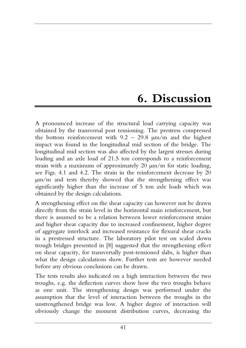
Figure A1 – Scaffolding for transversal drilling of the Haparanda Bridge.
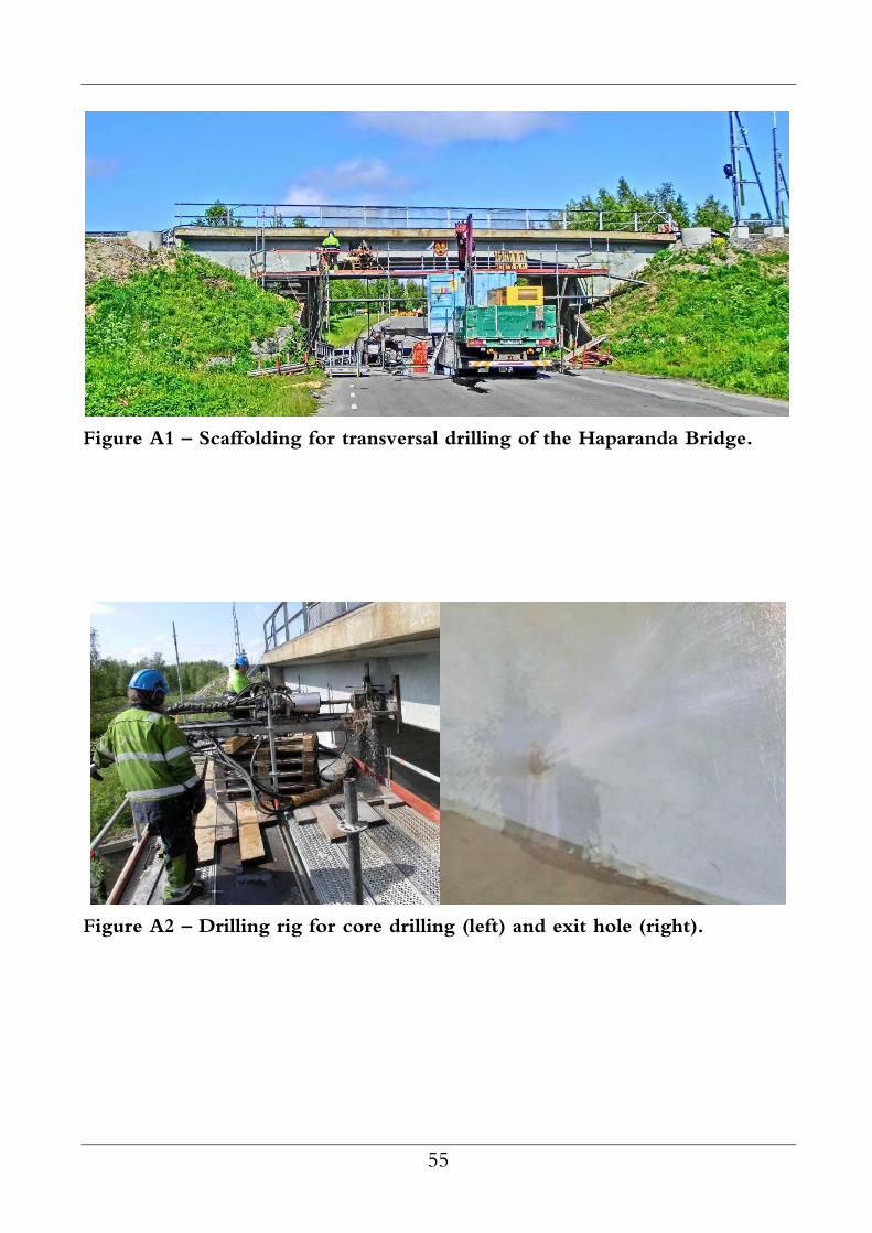
Figure A2 – Drilling rig for core drilling (left) and exit hole (right).

56
Figure A3 – Eight holes were drilled in the neutral layer of the slab of the Haparanda bridge.

57
Monitoring

58
Figure A4 – Rig for deflection monitoring. LVDTs are mounted onto the steel beams.
Figure A5 – SGs monitored the strain on the internal reinforcement (left) and prestressing bars (right).

59
Figure A6 – LVDTs monitored the deflections (left) and CODs monitored the transversal movement in the connection joint (right).

60
Strengthening

61
Figure A7 – A mechanical protection in the form of a PE duct was inserted into the hole (left) and a prestressing bar, protecting against corrosion by a heat shrinking sleeve, was inserted into the duct (right).
Figure A8 – A steel wedge acted as a load distributor and obtained a perpendicular contact against the concrete (left). The steel bars were
prestressed to 430 kN by a hydraulic jack (right).

62
Figure A9 – The prestressing system was finally sealed by a steel cap in order to obtain a sustainable strengthening solution.

63
Testing

64
Figure A10 – Two connected trains with 21.5 ton axle loads were used as loads during testing of the Haparanda Bridge.
Figure A11 – Railway traffic was not affected and could continue as the bridge was strengthened.

65
Appendix B – Test results

66
Strains

67
-40
-30
-20
-10
0
10
20
30
40
0 60 120 180 240 300 360 420 480
Str
ain
[µ
m/m
]
Time [s]
Strains (St1:1)
S1 S2
S3 S4
-40
-30
-20
-10
0
10
20
30
40
0 60 120 180 240
Str
ain
[µ
m/m
]
Time [s]
Strains (St1:2)
S1 S2
S3 S4
-40
-30
-20
-10
0
10
20
30
40
0 60 120 180 240 300
Str
ain
[µ
m/m
]
Time [s]
Strains (St2:1)
S1 S2
S3 S4
-40
-30
-20
-10
0
10
20
30
40
0 60 120 180 240 300
Str
ain
[µ
m/m
]
Time [s]
Strains (St2:2)
S1 S2
S3 S4
-40
-30
-20
-10
0
10
20
30
40
0 5 10 15 20 25 30 35 40 45
Str
ain
[µ
m/m
]
Time [s]
Strains (Dy1:1)
S1
-40
-30
-20
-10
0
10
20
30
40
0 5 10 15 20 25 30 35 40 45
Str
ain
[µ
m/m
]
Time [s]
Strains (Dy1:2)
S1

68
-40
-30
-20
-10
0
10
20
30
40
0 5 10 15 20 25 30 35 40 45
Str
ain
[µ
m/m
]
Time [s]
Strains (Dy1:1)
S2
-40
-30
-20
-10
0
10
20
30
40
0 5 10 15 20 25 30 35 40 45
Str
ain
[µ
m/m
]
Time [s]
Strains (Dy1:2)
S2
-40
-30
-20
-10
0
10
20
30
40
0 5 10 15 20 25 30 35 40 45
Str
ain
[µ
m/m
]
Time [s]
Strains (Dy1:1)
S3
-40
-30
-20
-10
0
10
20
30
40
0 5 10 15 20 25 30 35 40 45
Str
ain
[µ
m/m
]
Time [s]
Strains (Dy1:2)
S3
-40
-30
-20
-10
0
10
20
30
40
0 5 10 15 20 25 30 35 40 45
Str
ain
[µ
m/m
]
Time [s]
Strains (Dy1:1)
S4
-40
-30
-20
-10
0
10
20
30
40
0 5 10 15 20 25 30 35 40 45
Str
ain
[µ
m/m
]
Time [s]
Strains (Dy1:2)
S4

69
-40
-30
-20
-10
0
10
20
30
40
0 5 10 15 20 25 30 35 40 45
Str
ain
[µ
m/m
]
Time [s]
Strains (Dy2:1)
S1
-40
-30
-20
-10
0
10
20
30
40
0 5 10 15 20 25 30 35 40 45
Str
ain
[µ
m/m
]
Time [s]
Strains (Dy2:2)
S1
-40
-30
-20
-10
0
10
20
30
40
0 5 10 15 20 25 30 35 40 45
Str
ain
[µ
m/m
]
Time [s]
Strains (Dy2:1)
S2
-40
-30
-20
-10
0
10
20
30
40
0 5 10 15 20 25 30 35 40 45
Str
ain
[µ
m/m
]
Time [s]
Strains (Dy2:2)
S2
-40
-30
-20
-10
0
10
20
30
40
0 5 10 15 20 25 30 35 40 45
Str
ain
[µ
m/m
]
Time [s]
Strains (Dy2:1)
S3
-40
-30
-20
-10
0
10
20
30
40
0 5 10 15 20 25 30 35 40 45
Str
ain
[µ
m/m
]
Time [s]
Strains (Dy2:2)
S3

70
-40
-30
-20
-10
0
10
20
30
40
0 5 10 15 20 25 30 35 40 45
Str
ain
[µ
m/m
]
Time [s]
Strains (Dy2:1)
S4
-40
-30
-20
-10
0
10
20
30
40
0 5 10 15 20 25 30 35 40 45
Str
ain
[µ
m/m
]
Time [s]
Strains (Dy2:2)
S4
-40
-30
-20
-10
0
10
20
30
40
0 5 10 15 20 25 30 35
Str
ain
[µ
m/m
]
Time [s]
Strains (Dy3:1)
S1
-40
-30
-20
-10
0
10
20
30
40
0 5 10 15 20 25 30 35
Str
ain
[µ
m/m
]
Time [s]
Strains (Dy3:2)
S1
-40
-30
-20
-10
0
10
20
30
40
0 5 10 15 20 25 30 35
Str
ain
[µ
m/m
]
Time [s]
Strains (Dy3:1)
S2
-40
-30
-20
-10
0
10
20
30
40
0 5 10 15 20 25 30 35
Str
ain
[µ
m/m
]
Time [s]
Strains (Dy3:2)
S2

71
-40
-30
-20
-10
0
10
20
30
40
0 5 10 15 20 25 30 35
Str
ain
[µ
m/m
]
Time [s]
Strains (Dy3:1)
S3
-40
-30
-20
-10
0
10
20
30
40
0 5 10 15 20 25 30 35
Str
ain
[µ
m/m
]
Time [s]
Strains (Dy3:2)
S3
-40
-30
-20
-10
0
10
20
30
40
0 5 10 15 20 25 30 35
Str
ain
[µ
m/m
]
Time [s]
Strains (Dy3:1)
S4
-40
-30
-20
-10
0
10
20
30
40
0 5 10 15 20 25 30 35
Str
ain
[µ
m/m
]
Time [s]
Strains (Dy3:2)
S4
-40
-30
-20
-10
0
10
20
30
40
0 5 10 15 20 25 30 35
Str
ain
[µ
m/m
]
Time [s]
Strains (Dy4:1)
S1
-40
-30
-20
-10
0
10
20
30
40
0 5 10 15 20 25 30 35
Str
ain
[µ
m/m
]
Time [s]
Strains (Dy4:2)
S1

72
-40
-30
-20
-10
0
10
20
30
40
0 5 10 15 20 25 30 35
Str
ain
[µ
m/m
]
Time [s]
Strains (Dy4:1)
S2
-40
-30
-20
-10
0
10
20
30
40
0 5 10 15 20 25 30 35
Str
ain
[µ
m/m
]
Time [s]
Strains (Dy4:2)
S2
-40
-30
-20
-10
0
10
20
30
40
0 5 10 15 20 25 30 35
Str
ain
[µ
m/m
]
Time [s]
Strains (Dy4:1)
S3
-40
-30
-20
-10
0
10
20
30
40
0 5 10 15 20 25 30 35
Str
ain
[µ
m/m
]
Time [s]
Strains (Dy4:2)
S3
-40
-30
-20
-10
0
10
20
30
40
0 5 10 15 20 25 30 35
Str
ain
[µ
m/m
]
Time [s]
Strains (Dy4:1)
S4
-40
-30
-20
-10
0
10
20
30
40
0 5 10 15 20 25 30 35
Str
ain
[µ
m/m
]
Time [s]
Strains (Dy4:2)
S4

73
-40
-30
-20
-10
0
10
20
30
40
0 5 10 15 20 25
Str
ain
[µ
m/m
]
Time [s]
Strains (Dy5:1)
S1
-40
-30
-20
-10
0
10
20
30
40
0 5 10 15 20 25
Str
ain
[µ
m/m
]
Time [s]
Strains (Dy5:2)
S1
-40
-30
-20
-10
0
10
20
30
40
0 5 10 15 20 25
Str
ain
[µ
m/m
]
Time [s]
Strains (Dy5:1)
S2
-40
-30
-20
-10
0
10
20
30
40
0 5 10 15 20 25
Str
ain
[µ
m/m
]
Time [s]
Strains (Dy5:2)
S2
-40
-30
-20
-10
0
10
20
30
40
0 5 10 15 20 25
Str
ain
[µ
m/m
]
Time [s]
Strains (Dy5:1)
S3
-40
-30
-20
-10
0
10
20
30
40
0 5 10 15 20 25
Str
ain
[µ
m/m
]
Time [s]
Strains (Dy5:2)
S3

74
-40
-30
-20
-10
0
10
20
30
40
0 5 10 15 20 25
Str
ain
[µ
m/m
]
Time [s]
Strains (Dy5:1)
S4
-40
-30
-20
-10
0
10
20
30
40
0 5 10 15 20 25
Str
ain
[µ
m/m
]
Time [s]
Strains (Dy5:2)
S4
-40
-30
-20
-10
0
10
20
30
40
0 5 10 15 20 25
Str
ain
[µ
m/m
]
Time [s]
Strains (Dy6:1)
S1
-40
-30
-20
-10
0
10
20
30
40
0 5 10 15 20 25
Str
ain
[µ
m/m
]
Time [s]
Strains (Dy6:2)
S1
-40
-30
-20
-10
0
10
20
30
40
0 5 10 15 20 25
Str
ain
[µ
m/m
]
Time [s]
Strains (Dy6:1)
S2
-40
-30
-20
-10
0
10
20
30
40
0 5 10 15 20 25
Str
ain
[µ
m/m
]
Time [s]
Strains (Dy6:2)
S2

75
-40
-30
-20
-10
0
10
20
30
40
0 5 10 15 20 25
Str
ain
[µ
m/m
]
Time [s]
Strains (Dy6:1)
S3
-40
-30
-20
-10
0
10
20
30
40
0 5 10 15 20 25
Str
ain
[µ
m/m
]
Time [s]
Strains (Dy6:2)
S3
-40
-30
-20
-10
0
10
20
30
40
0 5 10 15 20 25
Str
ain
[µ
m/m
]
Time [s]
Strains (Dy6:1)
S4
-40
-30
-20
-10
0
10
20
30
40
0 5 10 15 20 25
Str
ain
[µ
m/m
]
Time [s]
Strains (Dy6:2)
S4
3900
4000
4100
0 60 120 180 240
Str
ain
[µ
m/m
]
Time [s]
PB-Strains (St1:2)
P1 P2
P3 P4
3900
4100
0 60 120 180 240 300
Str
ain
[µ
m/m
]
Time [s]
PB-Strains (St2:2)
P1 P2
P3 P4

76
3900
4100
0 5 10 15 20 25 30 35 40 45
Str
ain
[µ
m/m
]
Time [s]
PB-Strains (Dy1:2)
P1
3900
4100
0 5 10 15 20 25 30 35 40 45
Str
ain
[µ
m/m
]
Time [s]
PB-Strains (Dy1:2)
P2
3900
4100
0 5 10 15 20 25 30 35 40 45
Str
ain
[µ
m/m
]
Time [s]
PB-Strains (Dy1:2)
P3
3900
4100
0 5 10 15 20 25 30 35 40 45
Str
ain
[µ
m/m
]
Time [s]
PB-Strains (Dy1:2)
P4
3900
4100
0 5 10 15 20 25 30 35 40 45
Str
ain
[µ
m/m
]
Time [s]
PB-Strains (Dy2:2)
P1
3900
4100
0 5 10 15 20 25 30 35 40 45
Str
ain
[µ
m/m
]
Time [s]
PB-Strains (Dy2:2)
P2

77
3900
4100
0 5 10 15 20 25 30 35 40 45
Str
ain
[µ
m/m
]
Time [s]
PB-Strains (Dy2:2)
P3
3900
4100
0 5 10 15 20 25 30 35 40 45
Str
ain
[µ
m/m
]
Time [s]
PB-Strains (Dy2:2)
P4
3900
4100
0 5 10 15 20 25 30 35
Str
ain
[µ
m/m
]
Time [s]
PB-Strains (Dy3:2)
P1
3900
4100
0 5 10 15 20 25 30 35
Str
ain
[µ
m/m
]
Time [s]
PB-Strains (Dy3:2)
P2
3900
4100
0 5 10 15 20 25 30 35
Str
ain
[µ
m/m
]
Time [s]
PB-Strains (Dy3:2)
P3
3900
4100
0 5 10 15 20 25 30 35
Str
ain
[µ
m/m
]
Time [s]
PB-Strains (Dy3:2)
P4

78
3900
4100
0 5 10 15 20 25
Str
ain
[µ
m/m
]
Time [s]
PB-Strains (Dy4:2)
P1
3900
4100
0 5 10 15 20 25
Str
ain
[µ
m/m
]
Time [s]
PB-Strains (Dy4:2)
P2
3900
4100
0 5 10 15 20 25
Str
ain
[µ
m/m
]
Time [s]
PB-Strains (Dy4:2)
P3
3900
4100
0 5 10 15 20 25
Str
ain
[µ
m/m
]
Time [s]
PB-Strains (Dy4:2)
P4
3900
4100
0 5 10 15 20 25
Str
ain
[µ
m/m
]
Time [s]
PB-Strains (Dy5:2)
P1
3900
4100
0 5 10 15 20 25
Str
ain
[µ
m/m
]
Time [s]
PB-Strains (Dy5:2)
P2

79
3900
4100
0 5 10 15 20 25
Str
ain
[µ
m/m
]
Time [s]
PB-Strains (Dy5:2)
P3
3900
4100
0 5 10 15 20 25
Str
ain
[µ
m/m
]
Time [s]
PB-Strains (Dy5:2)
P4
3900
4100
0 5 10 15 20 25
Str
ain
[µ
m/m
]
Time [s]
PB-Strains (Dy6:2)
P1
3900
4100
0 5 10 15 20 25
Str
ain
[µ
m/m
]
Time [s]
PB-Strains (Dy6:2)
P2
3900
4100
0 5 10 15 20 25
Str
ain
[µ
m/m
]
Time [s]
PB-Strains (Dy6:2)
P3
3900
4100
0 5 10 15 20 25
Str
ain
[µ
m/m
]
Time [s]
PB-Strains (Dy6:2)
P4

80
Deflections

81
-0.1
0
0.1
0.2
0.3
0.4
0.5
0.6
0 60 120 180 240 300 360 420 480
Deflection [
mm
]
Time [s]
Deflections (St1:1)
L1 L2 L3
L4 L5 L6
-0.1
0
0.1
0.2
0.3
0.4
0.5
0.6
0 60 120 180 240
Deflection [
mm
]
Time [s]
Deflections (St1:2)
L1 L2 L3
L4 L5 L6
-0.1
0
0.1
0.2
0.3
0.4
0.5
0.6
0 60 120 180 240 300 360 420 480
Deflection [
mm
]
Time [s]
Deflections (St1:1)
L7 L8 L9
L10 L11
-0.1
0
0.1
0.2
0.3
0.4
0.5
0.6
0 60 120 180 240
Deflection [
mm
]
Time [s]
Deflections (St1:2)
L7 L8 L9
L10 L11
-0.1
0
0.1
0.2
0.3
0.4
0.5
0.6
0 60 120 180 240 300 360 420 480
Deflection [
mm
]
Time [s]
Deflections (St1:1)
L12 L13 L14
L15 L16
-0.1
0
0.1
0.2
0.3
0.4
0.5
0.6
0 60 120 180 240
Deflection [
mm
]
Time [s]
Deflections (St1:2)
L12 L13 L14
L15 L16

82
-0.1
0
0.1
0.2
0.3
0.4
0.5
0.6
0 60 120 180 240 300
Deflection [
mm
]
Time [s]
Deflections (St2:1)
L1 L2 L3
L4 L5 L6-0.1
0
0.1
0.2
0.3
0.4
0.5
0.6
0 60 120 180 240 300
Deflection [
mm
]
Time [s]
Deflections (St2:2)
L1 L2 L3
L4 L5 L6
-0.1
0
0.1
0.2
0.3
0.4
0.5
0.6
0 60 120 180 240 300
Deflection [
mm
]
Time [s]
Deflections (St2:1)
L7 L8 L9
L10 L11
-0.1
0
0.1
0.2
0.3
0.4
0.5
0.6
0 60 120 180 240 300
Deflection [
mm
]
Time [s]
Deflections (St2:2)
L7 L8 L9
L10 L11
-0.1
0
0.1
0.2
0.3
0.4
0.5
0.6
0 60 120 180 240 300
Deflection [
mm
]
Time [s]
Deflections (St2:1)
L12 L13 L14
L15 L16
-0.1
0
0.1
0.2
0.3
0.4
0.5
0.6
0 60 120 180 240 300
Deflection [
mm
]
Time [s]
Deflections (St2:2)
L12 L13 L14
L15 L16

83
-0.1
0
0.1
0.2
0.3
0.4
0.5
0.6
0 5 10 15 20 25 30 35 40 45
Deflection [
mm
]
Time [s]
Deflections (Dy1:1) L1
L2
L3
L4
L5
L6
-0.1
0
0.1
0.2
0.3
0.4
0.5
0.6
0 5 10 15 20 25 30 35 40 45
Deflection [
mm
]
Time [s]
Deflections (Dy1:2) L1
L2
L3
L4
L5
L6
-0.1
0
0.1
0.2
0.3
0.4
0.5
0.6
0 5 10 15 20 25 30 35 40 45
Deflection [
mm
]
Time [s]
Deflections (Dy1:1) L7
L8
L9
L10
L11
-0.1
0
0.1
0.2
0.3
0.4
0.5
0.6
0 5 10 15 20 25 30 35 40 45
Deflection [
mm
]
Time [s]
Deflections (Dy1:2) L7
L8
L9
L10
L11
-0.1
0
0.1
0.2
0.3
0.4
0.5
0.6
0 5 10 15 20 25 30 35 40 45
Deflection [
mm
]
Time [s]
Deflections (Dy1:1)
L12 L13 L14
L15 L16
-0.1
0
0.1
0.2
0.3
0.4
0.5
0.6
0 5 10 15 20 25 30 35 40 45
Deflection [
mm
]
Time [s]
Deflections (Dy1:2)
L12 L13 L14
L15 L16

84
-0.1
0
0.1
0.2
0.3
0.4
0.5
0.6
0 5 10 15 20 25 30 35 40 45
Deflection [
mm
]
Time [s]
Deflections (Dy2:1) L1
L2
L3
L4
L5
L6
-0.1
0
0.1
0.2
0.3
0.4
0.5
0.6
0 5 10 15 20 25 30 35 40 45
Deflection [
mm
]
Time [s]
Deflections (Dy2:2) L1
L2
L3
L4
L5
L6
-0.1
0
0.1
0.2
0.3
0.4
0.5
0.6
0 5 10 15 20 25 30 35 40 45
Deflection [
mm
]
Time [s]
Deflections (Dy2:1) L7
L8
L9
L10
L11
-0.1
0
0.1
0.2
0.3
0.4
0.5
0.6
0 5 10 15 20 25 30 35 40 45
Deflection [
mm
]
Time [s]
Deflections (Dy2:2) L7
L8
L9
L10
L11
-0.1
0
0.1
0.2
0.3
0.4
0.5
0.6
0 5 10 15 20 25 30 35 40 45
Deflection [
mm
]
Time [s]
Deflections (Dy2:1)
L12 L13 L14
L15 L16
-0.1
0
0.1
0.2
0.3
0.4
0.5
0.6
0 5 10 15 20 25 30 35 40 45
Deflection [
mm
]
Time [s]
Deflections (Dy2:2)
L12 L13 L14
L15 L16

85
-0.1
0
0.1
0.2
0.3
0.4
0.5
0.6
0 5 10 15 20 25 30 35
Deflection [
mm
]
Time [s]
Deflections (Dy3:1) L1
L2
L3
L4
L5
L6
-0.1
0
0.1
0.2
0.3
0.4
0.5
0.6
0 5 10 15 20 25 30 35
Deflection [
mm
]
Time [s]
Deflections (Dy3:2) L1
L2
L3
L4
L5
L6
-0.1
0
0.1
0.2
0.3
0.4
0.5
0.6
0 5 10 15 20 25 30 35
Deflection [
mm
]
Time [s]
Deflections (Dy3:1) L7
L8
L9
L10
L11
-0.1
0
0.1
0.2
0.3
0.4
0.5
0.6
0 5 10 15 20 25 30 35
Deflection [
mm
]
Time [s]
Deflections (Dy3:2) L7
L8
L9
L10
L11
-0.1
0
0.1
0.2
0.3
0.4
0.5
0.6
0 5 10 15 20 25 30 35
Deflection [
mm
]
Time [s]
Deflections (Dy3:1)
L12 L13 L14
L15 L16
-0.1
0
0.1
0.2
0.3
0.4
0.5
0.6
0 5 10 15 20 25 30 35
Deflection [
mm
]
Time [s]
Deflections (Dy3:2)
L12 L13 L14
L15 L16

86
-0.1
0
0.1
0.2
0.3
0.4
0.5
0.6
0 5 10 15 20 25 30 35
Deflection [
mm
]
Time [s]
Deflections (Dy4:1) L1
L2
L3
L4
L5
L6
-0.1
0
0.1
0.2
0.3
0.4
0.5
0.6
0 5 10 15 20 25 30 35
Deflection [
mm
]
Time [s]
Deflections (Dy4:2) L1
L2
L3
L4
L5
L6
-0.1
0
0.1
0.2
0.3
0.4
0.5
0.6
0 5 10 15 20 25 30 35
Deflection [
mm
]
Time [s]
Deflections (Dy4:1) L7
L8
L9
L10
L11
-0.1
0
0.1
0.2
0.3
0.4
0.5
0.6
0 5 10 15 20 25 30 35
Deflection [
mm
]
Time [s]
Deflections (Dy4:2) L7
L8
L9
L10
L11
-0.1
0
0.1
0.2
0.3
0.4
0.5
0.6
0 5 10 15 20 25 30 35
Deflection [
mm
]
Time [s]
Deflections (Dy4:1)
L12 L13 L14
L15 L16
-0.1
0
0.1
0.2
0.3
0.4
0.5
0.6
0 5 10 15 20 25 30 35
Deflection [
mm
]
Time [s]
Deflections (Dy4:2)
L12 L13 L14
L15 L16

87
-0.1
0
0.1
0.2
0.3
0.4
0.5
0.6
0 5 10 15 20 25
Deflection [
mm
]
Time [s]
Deflections (Dy5:1) L1
L2
L3
L4
L5
L6
-0.1
0
0.1
0.2
0.3
0.4
0.5
0.6
0 5 10 15 20 25
Deflection [
mm
]
Time [s]
Deflections (Dy5:2) L1
L2
L3
L4
L5
L6
-0.1
0
0.1
0.2
0.3
0.4
0.5
0.6
0 5 10 15 20 25
Deflection [
mm
]
Time [s]
Deflections (Dy5:1) L7
L8
L9
L10
L11
-0.1
0
0.1
0.2
0.3
0.4
0.5
0.6
0 5 10 15 20 25
Deflection [
mm
]
Time [s]
Deflections (Dy5:2) L7
L8
L9
L10
L11
-0.1
0
0.1
0.2
0.3
0.4
0.5
0.6
0 5 10 15 20 25
Deflection [
mm
]
Time [s]
Deflections (Dy5:1)
L12 L13 L14
L15 L16
-0.1
0
0.1
0.2
0.3
0.4
0.5
0.6
0 5 10 15 20 25
Deflection [
mm
]
Time [s]
Deflections (Dy5:2)
L12 L13 L14
L15 L16

88
-0.1
0
0.1
0.2
0.3
0.4
0.5
0.6
0 5 10 15 20 25
Deflection [
mm
]
Time [s]
Deflections (Dy6:1) L1
L2
L3
L4
L5
L6
-0.1
0
0.1
0.2
0.3
0.4
0.5
0.6
0 5 10 15 20 25
Deflection [
mm
]
Time [s]
Deflections (Dy6:2) L1
L2
L3
L4
L5
L6
-0.1
0
0.1
0.2
0.3
0.4
0.5
0.6
0 5 10 15 20 25
Deflection [
mm
]
Time [s]
Deflections (Dy6:1) L7
L8
L9
L10
L11
-0.1
0
0.1
0.2
0.3
0.4
0.5
0.6
0 5 10 15 20 25
Deflection [
mm
]
Time [s]
Deflections (Dy6:2) L7
L8
L9
L10
L11
-0.1
0
0.1
0.2
0.3
0.4
0.5
0.6
0 5 10 15 20 25
Deflection [
mm
]
Time [s]
Deflections (Dy6:1)
L12 L13 L14
L15 L16
-0.1
0
0.1
0.2
0.3
0.4
0.5
0.6
0 5 10 15 20 25
Deflection [
mm
]
Time [s]
Deflections (Dy6:2)
L12 L13 L14
L15 L16

89
Joint opening

90
-0.004
0
0.004
0 60 120 180 240 300 360 420 480
Movem
ent
[mm
]
Time [s]
COD (St1:1)
C1 C2 C3
-0.004
0
0.004
0 60 120 180 240
Movem
ent
[mm
]
Time [s]
COD (St1:2)
C1 C2 C3
-0.004
0
0.004
0 60 120 180 240 300
Movem
ent
[mm
]
Time [s]
COD (St2:1)
C1 C2 C3
-0.004
0
0.004
0 60 120 180 240 300
Movem
ent
[mm
]
Time [s]
COD (St2:2)
C1 C2 C3
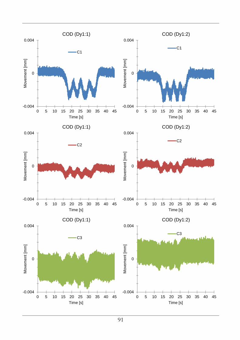
91
-0.004
0
0.004
0 5 10 15 20 25 30 35 40 45
Movem
ent
[mm
]
Time [s]
COD (Dy1:1)
C1
-0.004
0
0.004
0 5 10 15 20 25 30 35 40 45
Movem
ent
[mm
]
Time [s]
COD (Dy1:2)
C1
-0.004
0
0.004
0 5 10 15 20 25 30 35 40 45
Movem
ent
[mm
]
Time [s]
COD (Dy1:1)
C2
-0.004
0
0.004
0 5 10 15 20 25 30 35 40 45
Movem
ent
[mm
]
Time [s]
COD (Dy1:2)
C2
-0.004
0
0.004
0 5 10 15 20 25 30 35 40 45
Movem
ent
[mm
]
Time [s]
COD (Dy1:1)
C3
-0.004
0
0.004
0 5 10 15 20 25 30 35 40 45
Movem
ent
[mm
]
Time [s]
COD (Dy1:2)
C3

92
-0.004
0
0.004
0 5 10 15 20 25 30 35 40 45
Movem
ent
[mm
]
Time [s]
COD (Dy2:1)
C1
-0.004
0
0.004
0 5 10 15 20 25 30 35 40 45
Movem
ent
[mm
]
Time [s]
COD (Dy2:2)
C1
-0.004
0
0.004
0 5 10 15 20 25 30 35 40 45
Movem
ent
[mm
]
Time [s]
COD (Dy2:1)
C2
-0.004
0
0.004
0 5 10 15 20 25 30 35 40 45
Movem
ent
[mm
]
Time [s]
COD (Dy2:2)
C2
-0.004
0
0.004
0 5 10 15 20 25 30 35 40 45
Movem
ent
[mm
]
Time [s]
COD (Dy2:1)
C3
-0.004
0
0.004
0 5 10 15 20 25 30 35 40 45
Movem
ent
[mm
]
Time [s]
COD (Dy2:2)
C3
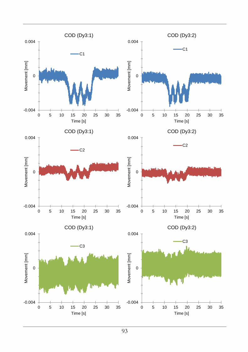
93
-0.004
0
0.004
0 5 10 15 20 25 30 35
Movem
ent
[mm
]
Time [s]
COD (Dy3:1)
C1
-0.004
0
0.004
0 5 10 15 20 25 30 35
Movem
ent
[mm
]
Time [s]
COD (Dy3:2)
C1
-0.004
0
0.004
0 5 10 15 20 25 30 35
Movem
ent
[mm
]
Time [s]
COD (Dy3:1)
C2
-0.004
0
0.004
0 5 10 15 20 25 30 35
Movem
ent
[mm
]
Time [s]
COD (Dy3:2)
C2
-0.004
0
0.004
0 5 10 15 20 25 30 35
Movem
ent
[mm
]
Time [s]
COD (Dy3:1)
C3
-0.004
0
0.004
0 5 10 15 20 25 30 35
Movem
ent
[mm
]
Time [s]
COD (Dy3:2)
C3

94
-0.004
0
0.004
0 5 10 15 20 25 30 35
Movem
ent
[mm
]
Time [s]
COD (Dy4:1)
C1
-0.004
0
0.004
0 5 10 15 20 25 30 35
Movem
ent
[mm
]
Time [s]
COD (Dy4:2)
C1
-0.004
0
0.004
0 5 10 15 20 25 30 35
Movem
ent
[mm
]
Time [s]
COD (Dy4:1)
C2
-0.004
0
0.004
0 5 10 15 20 25 30 35
Movem
ent
[mm
]
Time [s]
COD (Dy4:2)
C2
-0.004
0
0.004
0 5 10 15 20 25 30 35
Movem
ent
[mm
]
Time [s]
COD (Dy4:1)
C3
-0.004
0
0.004
0 5 10 15 20 25 30 35
Movem
ent
[mm
]
Time [s]
COD (Dy4:2)
C3

95
-0.004
0
0.004
0 5 10 15 20 25
Movem
ent
[mm
]
Time [s]
COD (Dy5:1)
C1
-0.004
0
0.004
0 5 10 15 20 25
Movem
ent
[mm
]
Time [s]
COD (Dy5:2)
C1
-0.004
0
0.004
0 5 10 15 20 25
Movem
ent
[mm
]
Time [s]
COD (Dy5:1)
C2
-0.004
0
0.004
0 5 10 15 20 25
Movem
ent
[mm
]
Time [s]
COD (Dy5:2)
C2
-0.004
0
0.004
0 5 10 15 20 25
Movem
ent
[mm
]
Time [s]
COD (Dy5:1)
C3
-0.004
0
0.004
0 5 10 15 20 25
Movem
ent
[mm
]
Time [s]
COD (Dy5:2)
C3
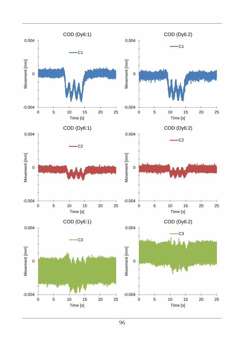
96
-0.004
0
0.004
0 5 10 15 20 25
Movem
ent
[mm
]
Time [s]
COD (Dy6:1)
C1
-0.004
0
0.004
0 5 10 15 20 25
Movem
ent
[mm
]
Time [s]
COD (Dy6:2)
C1
-0.004
0
0.004
0 5 10 15 20 25
Movem
ent
[mm
]
Time [s]
COD (Dy6:1)
C2
-0.004
0
0.004
0 5 10 15 20 25
Movem
ent
[mm
]
Time [s]
COD (Dy6:2)
C2
-0.004
0
0.004
0 5 10 15 20 25
Movem
ent
[mm
]
Time [s]
COD (Dy6:1)
C3
-0.004
0
0.004
0 5 10 15 20 25
Movem
ent
[mm
]
Time [s]
COD (Dy6:2)
C3

97
Appendix C – Design calculations

98
Shear capacity
The calculations performed by WSP (2008) page 5.54 shows a total shear
capacity of 150kN in the critical section (x = 2.998 m). The degree of utilization is 1.24, which implies a shear force of kN. 186150241 . The required shear force
to be taken by the strengthening system is therefore 36 kN.
Eurocode
The shear resistance of the prestressing can be calculated as:
dbσkV wcpRd,P 1
where
NN
bh
Nσcp 5.2
0.14.0
0.1wb
372.0d
15.01 k
The shear contribution from the prestress is thereby:
NNdbσkV wcpRd,P 1395.0372.015.215.01
The required shear contribution from the prestress is 36 kN, which is equal to a prestressing force of:
mkNV
N P / 2581395.0
36
1395.0

99
Final shear capacity
A strengthening system which introduces a normal force of 286 kN/m was chosen.
The shear contribution from the prestress is:
NNdbσkV wcpRd,P 1395.0372.015.215.01
When a normal force of 286 kN/m is intruduced, the corresponding increase in shear capacity will be
mkNNVRd,P / 9.392860001395.01395.0
The total shear capacity will be 150 + 39.9 = 189.9 kN/m

100
Flexural capacity
Figure C1 – Forces acting on a prestressed cross section.
Assuming yielding in the tensile reinforcement, the horizontal equilibrium
equation will be:
0' SSC FPFF
The compressive reinforcement is neglected, yielding is assumed in the tensile
reinforcement and the concrete reaches the ultimate compressive strain. The previous equation can then be developed into:
08.0 Sstcc AfPbxf
The distance to the neutral layer, x, can be solved with the following equation:
1
2
C
Cx
where
1032010009.128.08.01 bfC cc

101
Unstrengthened flexural capacity
76562725771.29702 Sst AfPC
mmx 2.7410320
765627
Through moment equilibrium around the concrete resultant force the following equation is obtained
04.02
4.0
Mx
hPxdFS
where the flexural capacity can be solved as
x
hPxdAfM Sst 4.0
24.0
mkNmM / 2572.744.036625771.297

102
Strengthened flexural capacity
A normal force of 286 kN/m is introduced as strengthening, giving the following equations
105162725771.2972860002 Sst AfPC
mmx 9.10110320
1051627
Through moment equilibrium around the concrete resultant force the following
equation is obtained
04.02
4.0
Mx
hPxdFS
where the flexural capacity can be solved as
x
hPxdAfM Sst 4.0
24.0
mkNmM
M
/ 295
109.1014.02
400286000109.1014.036625771.297 33
The obtained capacity of 295 kNm/m can be compared to the required flexural capacity 368 kNm/m.
The strain in the reinforcement will be
071.95.3
9.101
9.101366cuS
x
xd
298.25.3
9.101
359.101'' cuS
x
dx
This means that compressive and tensile reinforcement are yielding at ultimate
limit state.
S
st
cu
cu
E
fd
x
10.1
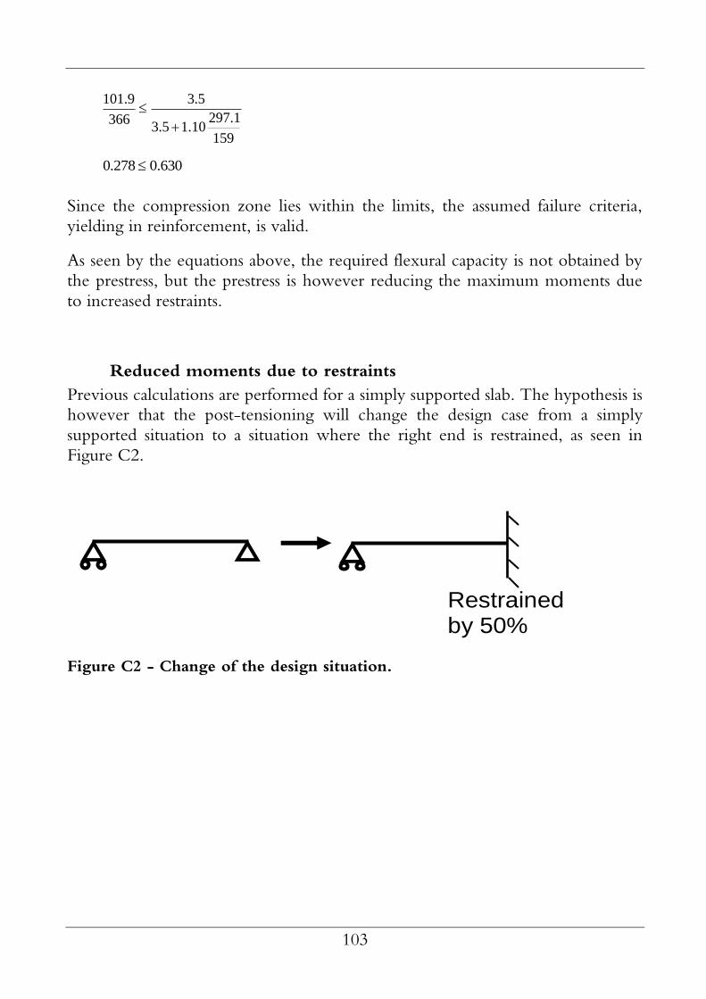
103
159
1.29710.15.3
5.3
366
9.101
630.0278.0
Since the compression zone lies within the limits, the assumed failure criteria,
yielding in reinforcement, is valid.
As seen by the equations above, the required flexural capacity is not obtained by
the prestress, but the prestress is however reducing the maximum moments due
to increased restraints.
Reduced moments due to restraints
Previous calculations are performed for a simply supported slab. The hypothesis is however that the post-tensioning will change the design case from a simply
supported situation to a situation where the right end is restrained, as seen in
Figure C2.
Restrained by 50%
Figure C2 - Change of the design situation.

104
Figure C.3 shows the moment distribution in the transversal direction for a
simply supported slab and a slab with 50% degree of restraint.
Figure C3 – Transversal moment distribution [Nm/m] for a simply supported slab (left) and a slab were the right end is restrained by 50%
(right).
The maximum design moment decreases from 368 kNm/m to 280 kNm/m and the capacity of 295 kNm/m for the strengthened beam is thereby sufficient.
Only Load Combination A in WSP (2008) is considered, were the total load is
trafficballastconcretetot qqqq 4.11.1

105
Distribution wedges
The contact between the prestressing system and the concrete structure requires
being perpendicular to ensure an effective stress transfer from the prestressing bars to the concrete structure. Since the holes were drilled with an angle of 73°,
instead of 90°, a galvanized steel wedge was specially designed to obtain the required perpendicularity. The wedges also functioned as load distributors,
distributing the prestressing force over a larger concrete area and preventing local
concrete crushing or splitting behind the post-tensioning anchors.
As a simplification, Eurocode states that the prestressing force may be assumed to
disperse at an angle of 2 , starting at the end of the anchoring device. The value
of is assumed to be 7.333
2arctan .
The prestressing force is transferred from the bar, through the anchor plate and
the distribution wedge, onto the concrete structure. The external main girder of
the trough bridge has a width of 857 mm and is assumed to act as a load distribution device for the concrete slab. The force is dispersed over a distance of
571 mm by passing through the girder and if the c/c distance for the prestressing bars is chosen as 1500 mm, the required width of the distribution wedge will
become mm 35857121500 .
A width of 382 mm was finally chosen for the distribution wedges, as seen in Figure C4.
Figure C4 – Load distribution through the main girders. All measurements
are given in mm.