1

Joop’s World: The Analog Earth Model

By Beth Ogata, Olivia Miller, Susanna Ronalds-Hanna, and Tanya Harrison INTRODUCTION Global warming is one of the biggest issues in the global consciousness today, acknowledged more and more as a legitimate and grave threat and defining our generation by the way we choose to address the problem. Respected scientific opinion has attributed the accelerating influx of carbon dioxide gas from anthropogenic sources as a primary factor behind the rising global mean temperature, accelerated melting of polar ice sheets, and other environmental anomalies.

The purpose of the analog Earth experiment was to understand energy fluxes and heat balances in the Earth system. As an analog of the Earth, Joop’s World removed spatial complexity and extraneous influencing variables found in the Earth’s system. This simplified model gave data on the fundamental processes dictating climate. We examined the effect of carbon dioxide as a greenhouse gas in order to gain insight on the effects of increasing CO2 on the actual Earth system. Our results tentatively identified CO2 as a greenhouse gas, as it contributes to the reequilibration of our small-scale Earth system at a higher temperature than did the radiatively neutral gas nitrogen. Also, increased concentrations of CO2 caused the equilibrium temperature to increase. However, the thermal properties of radiatively neutral argon interfered with the analog greenhouse effect.

The way in which the role of convection was expressed in Joop’s World lead to

curious results and thus exposed the limitations of our analog model. Although initially the focus of the experiment was on the role of carbon dioxide as a greenhouse gas and the influence of concentration on equilibrium temperature, as the experiment progressed, convective cooling proved to be an unanticipated, yet significant, interesting influencing force and became an additional focus of the experiment. The role of convection in the Earth system’s heat balance is relevant as skeptics of global climate change argue that with increased warming due to higher concentrations of greenhouse gases, the kinetic energy associated with higher temperatures will be negated by a simultaneous increase in planetary cooling mechanisms such a convective cooling (Dr. Johan Varekamp, personal communication). BACKGROUND As an analog Earth model, Joop’s World attempted to simulate the energy balance of the Earth system. The amount of heat received and distributed by the Earth ultimately dictates Earth’s climate. Important factors influencing the Earth’s heat budget are the amount of solar energy input and spectral distribution, distance from the sun, reflectivity of the Earth, atmospheric absorption of incoming radiation, greenhouse effect and convective heat flux.

2

With Joop’s World, the aim was to observe and manipulate the greenhouse effect on a more manageable scale. The Earth, a blackbody, receives radiation emitted by the sun. In turn, the Earth emits electromagnetic radiation. The amount of energy given off by the sun can be calculated using Planck’s Law, which describes the wavelength distribution of electromagnetic radiation for a given temperature of a blackbody. The Stefan-Boltzmann Law integrates Planck’s Law over wavelength to hold that the amount of radiation emitted by an object at a given temperature is proportional to the fourth power of its temperature. Wien’s Law takes the derivative of Planck’s Law to find the wavelength of peak emission for a blackbody at a given temperature.

Planck’s Law Bλ(λ, T) dλ = {(2hc2) / λ5}x{1/ [e^(ch/ kλT)-1] } dλ

where λ = wavelength (meters) and T = temperature (Kelvin)

Stefan-Boltzmann Law

E=σεT4 Stefan-Boltzmann constant: σ = 5.67x10-8 W m-2 K-4

ε = Emissivity

Wien’s Law λ = 0.003/T

(Dr. Varekamp’s lecture notes, 1/29/2008)

Boltzmann’s Law can then be used to calculate the flux of solar energy. The radiative terrestrial temperature can be calculated assuming a state of radiative equilibrium in which the amount of energy received by a system is equal to the amount of energy leaving the system. In this steady state condition in which the incoming radiation is equal to the outgoing radiation, the Earth’s temperature can be calculated using the following equation:

(1-α)S*=σTs4

α = total planetary albedo S = Solar constant

Of the energy that reaches Earth’s atmosphere, approximately 31% is reflected

back into space due to the high albedo of ice, water, clouds and aerosols (Dr. Varekamp’s lecture notes, 1/31/2008). The Earth absorbs the remaining energy and then radiates infrared radiation of about 4-40 mm with the most intense wavelength at about 11 mm, as dictated by Wien’s Law. Using this radiative equilibrium equation, the Earth’s temperature is calculated to be 255 K (-18 ºC), much colder than the mean annual temperature on Earth of 288 K (15 °C). This discrepancy is due to the greenhouse effect in which greenhouse gases in the troposphere absorb long-wavelength, infrared terrestrial radiation and reradiates the energy in all directions, including back to Earth’s surface. This results in the Earth heating up and reradiating more energy to maintain radiative equilibrium. The greenhouse effect can be conceptualized as the transmissivity of the

3

atmosphere. The transmissivity of the atmosphere is approximately 60% and can be included in the heat balance equation as τ.

(1-α)S*=τσTs

4 τ = transmissivity (analog for the greenhouse effect)

(Dr. Varekamp’s lecture notes, 1/31/2008)

Accounting for the absorption and reradiation of terrestrial energy, the calculated Earth temperature is 288 K (15 °C). Thus, the greenhouse effect is responsible for a 33 °C increase in Earth’s temperature. Greenhouse gases include water vapor, carbon dioxide, methane, nitrous oxide, chlorofluorocarbons (CFC) and ozone. These gases have an odd number of atoms and thus an oscillating dipole moment which allows them to absorb infrared radiation at a wavelength or multiple wavelengths characteristic to the specific gas (Fig. 1). Upon absorption of the outgoing terrestrial radiation of a specific wavelength, the molecules vibrate more energetically and their energy content increases. The molecule gives up this energy by colliding with another molecule and transferring the vibrational energy to the other molecule. Alternatively, the molecule can spontaneously emit energy in the form of a photon. This photon can be emitted in any direction so that it may be absorbed by another molecule, escape to space, or return to Earth.

Figure 1: Absorption spectrum of greenhouse gases. Source:

jvarekamp.web.wesleyan.edu/CO2/359%20CC%2008/whole%20spectr.jpg Most interest in the greenhouse effect has focused on the role of carbon dioxide as a greenhouse gas. The atmosphere contains approximately 380 ppmv of carbon dioxide. Carbon dioxide is intimately linked with the carbon cycle. It may be removed from the atmosphere by photosynthesis, chemical weathering of minerals, and dissolution in the oceans and is released into the atmosphere by respiration, exsolution from water, volcanoes and forest fires. In recent history the cycle maintained a relatively stable

4

carbon dioxide influx and outflux with the atmosphere. However, anthropogenic combustion of fossil fuels is becoming an increasingly added source of carbon dioxide into the atmosphere. Air trapped in polar ice shows that before the start of the industrial era in 1800, atmospheric carbon dioxide concentration was between 275-280 ppmv. The Keeling curve shows concentrations of atmospheric carbon dioxide from the Mauna Loa Observatory in Hawaii from 1958 to the present (Fig. 2). The measurements show an increase in concentration from 315 ppmv in 1958 to over 380 ppmv in 2006 (Dr. Varekamp’s lecture notes, 2/21/2008). Seasonal plant growth cycles account for the oscillations. Joop’s World does not account for carbon cycling processes.

Figure 2: Source: http://www.oar.noaa.gov/spotlite/archive/spot_jimomedal.html

Climate sensitivity calculates the global mean temperature increase required to

restore radiative equilibrium with a doubling of the concentration of carbon dioxide in the atmosphere. Calculated estimates of this parameter range from 1.5-4.5 °C as calculations account for various feedbacks to different extents (Dr. Varekamp’s lecture notes, 2/12/2008). Some feedbacks include the possible greening of the Earth in which higher levels of atmospheric carbon dioxide increase the rate of photosynthesis, causing a slight drawdown of carbon dioxide into terrestrial biomass. Additionally, higher atmospheric concentrations of carbon dioxide may result in a higher dissolution rate of carbon dioxide into the oceans. Although the analog Earth model does not take into account these feedback loops, the results were able to register a certain climate sensitivity of the model in terms of the relationship between CO2 added and the associated increase in radiative equilibrium temperature (Dr. Varekamp’s lecture notes, 2/12/2008).

Convection is the transfer of heat by the movement of a fluid such as a liquid or

gas. Upon heating, the fluid expands and its density decreases. The buoyant forces drive the fluid upward due to its lower pressure while a viscous force opposes this motion. Convection sets in when the buoyant force exceeds the viscous force and can be assessed using principles of Rayleigh-Bénard convection in which the Rayleigh number is the critical value at which convection begins.

5

kvgdRa

4αβ=

Ra = ratio of buoyant to viscous force

g= acceleration due to gravity α = coefficient of thermal expansion

β = temperature gradient d = depth chamber

k = thermal diffusivity v = kinematic viscosity

(Source: Ghorai 2003)

Although convective cooling was found to be a larger component than expected in Joop’s World, convection is also an important process on Earth. Large convective cells form on Earth due to uneven heating by the sun. While the equator receives sunlight at a near 90° angle, the poles receive sunlight at a much larger angle of incidence. The energy is thus spread out over a larger surface area at the poles than at the equator. Convective cells transport the heat from the equator towards the pole. The Earth is cooled by these convective cells as heat is carried up into the atmosphere where it can be radiated to outer space. However, convection cannot completely offset an increase in temperature because heat cannot be completely transferred into work and no system is 100% efficient per the 2nd Law of Thermodynamics (Dr. Varekamp’s lecture notes, 2/14/2008).

The Earth’s temperature is ultimately dictated by a balance and flow of heat into,

out of, and within the Earth system. This experiment specifically focuses on the effect of carbon dioxide gas at two concentrations (room air and pure CO2; exact concentrations were not measured) on the temperature of the Earth and its atmosphere. As Joop’s World is a small-scale analog model, radiative equilibrium temperatures reached will not be comparable to those of the Earth. However, by comparing the temperature response of the analog Earth to CO2, argon, nitrogen, ambient air, and low pressure, the effects of increasing CO2 concentrations in the Earth’s atmosphere can be evaluated quantitatively. Nitrogen and argon were chosen as comparison gases because they are radiatively neutral in the infrared. The low pressure runs were attempts at a vacuum in order to have a blank baseline run to compare the different gases to. METHODS

The machine shop constructed an aluminum two-layered cylindrical chamber measuring 22.5 cm tall and 23.5 cm in diameter, with a volume of 9759.1 cm3 (Fig. 3). The chamber sits on three legs. Inside of the inner chamber, a metal sphere sits on a thermally insulated stem. Two different spheres were used, one composed of brass and the other of aluminum. The brass ball measured 37 mm in diameter and weighed 101.5 g (ball and stem together weighed 107.5 g). The aluminum ball measured 37 mm and weighed 30.44 g. There is one circular window on each side, 180° from each other, which look into the inner chamber. The windows are condenser lenses from a petrologic microscope. No infrared light passes through these windows, and therefore no heat is

6

imparted upon or lost from the system inside the chamber via the windows. There is also a small window on the top of the chamber that is made of KBr that allows infrared radiation to pass through so that spectroscopy work could be performed. The inner chamber has input and output pipes for gasses while the outer chamber has input and output pipes for water, used to remove heat from the inner chamber. Thermocouples were placed inside the metal ball, floating in the chamber, touching the wall of the chamber, and outside in the room. The whole apparatus was insulated with two layers of closed cell foam with an R value of approximately 5.5 per inch in order to minimize heat lost from the system.

Figure 3: Schematic of Joop's World. Not all features shown were actually used, such as the water

cooling feature. First, either 250 W or 150 W halogen lights were directed through the windows

and focused on the ball inside the inner chamber, mimicking the sun shining on the Earth. Care was used to focus the lights directly on the ball to concentrate all energy from the lights onto the blackbody. A volume absorbing colorimeter was used to measure the power from the lights coming into the chamber. 0.7 W arrived in the chamber from the left light and 0.55 W arrived in the chamber from the right light, for a total of 1.25 W shining on the metal ball (a 1% yield). Then the lights were turned off to prevent heating of the ball and different gases were flushed into the inner chamber for each run. The gases used were ambient air, CO2, argon, and nitrogen. Gases were successively flushed into the chamber for 5 minutes at a rate of 7 cubic feet per minute and allowed to equilibrate with room pressure. For one experiment, a vacuum with an initial pressure of 23 inch Hg was attempted, and maintained between 15 and 20 inch Hg, by sealing a thermocouple into the post with epoxy and refreshing the vacuum periodically. Finally, the lights were turned on and the temperature of each thermocouple was recorded using a computer program called LoggerPro3. The lights were left on as long as necessary until the temperature of the ball reached a plateau at equilibrium, usually approximately two to three hours. The various runs were conducted as follows:

7

Table 1: Experimental Runs

Date Gases in Chamber Light Power Ball Material 4/9/08 Air, CO2 250 W Brass 4/10/08 Air 250 W Brass 4/14/08 Air, CO2 150 W Brass 4/15/08 Argon 250 W Brass 4/18/08 Argon, CO2 150 W Brass 4/21/08 CO2, Nitrogen 150 W Brass 4/22/08 Air 150 W Aluminum 4/23/08 Air, CO2, Nitrogen,

Argon 150 W Aluminum

4/24/08 Low pressure, Air 150 W Aluminum

The experiment initially began with 250 W bulbs, but due to problems with the bulbs burning out before the sphere inside the chamber had reached radiative equilibrium, they were replaced with 150 W bulbs. The brass sphere was replaced with an aluminum run due to the higher heat capacity of aluminum. Since the water jacket was not utilized, convection ended up playing a larger role than expected, and once this was realized, a thermocouple was placed inside the chamber to measure the temperature of the atmosphere (in addition to the three original thermocouples in the sphere, on the wall, and in the room to measure ambient temperature). Therefore, some of the runs had temperature data from three thermocouples while the later runs had data from four. The thermocouple on the wall allowed for calculation of the radiation flux from the wall. ENERGY BALANCE

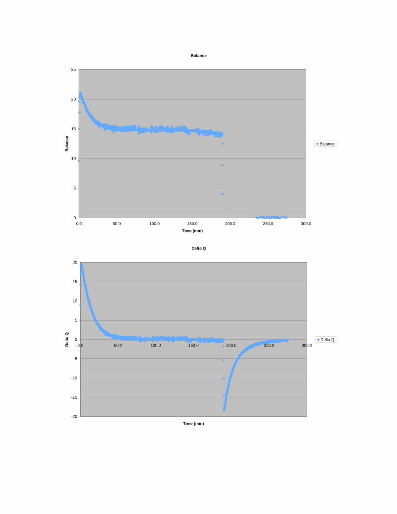
The energy balance in the sphere was assessed by grouping the energy inputs in the sphere and outputs from the sphere together. The energy from the lamps was a source of energy into the sphere. Additionally, as the cell heated up, the walls became warmer and also radiated energy back to the sphere. In the future, the walls can be cooled by running ice cold water through the water jackets to remove the heat from the walls and prevent their radiation of energy. However, in this experiment, the radiation of the walls was factored into the calculations. The sphere released energy by radiative and convective cooling mechanisms. Thus, the energy flux (ΔQ) of the system is equal to the amount of energy put in minus the amount of energy that flows out.

ΔQ = Qin - Qout

Qlamp + Qwall = Qradiation + Qconvective At radiative equilibrium ΔQ = 0

(Q = heat energy)

At the beginning of a run the lamps were turned on and the sphere heated up. At this point of the energy flux is positive because the amount of energy entering the sphere is greater than the amount leaving the sphere. Once the sphere heated up, it established radiative equilibrium, where the amount of energy entering the sphere equals the amount of energy leaving. At this point the temperature of the sphere should be constant and can be measured directly by a thermocouple within the sphere or calculated by analyzing the

8

fluxes of energy into and out of the sphere. When a greenhouse gas such as carbon dioxide is added, it is expected by the principles of the greenhouse effect, that a portion of the infrared energy radiated by the sphere will be reradiated back to the sphere. This added influx of energy will raise the temperature of the sphere which will then radiate more energy to reestablish radiative equilibrium at a higher temperature. The cooling curve was assessed by turning off the lamps and analyzing the decreasing temperature of the sphere. At this point, the energy flux is negative as the input from the lights is zero and the sphere is radiating energy until it reaches equilibrium with the ambient temperature. The cooling mechanisms of the sphere were radiation and convection.

RESULTS AND DISCUSSION

Table 2: Maximum Temperatures in Experimental Runs

Date Light Power

Ball Material Gases in Chamber

Ball Tmax, Gas 1 (°C)

Ball Tmax, Gas 2 (°C)

Ball Tmax, Gas 3 (°C)

Ball Tmax, Gas 4 (°C)

Tmax, Atmos (°C)

4/9/08 250 W Brass Air->CO2 64.84 66.46 -- -- 29.00 4/10/08 250 W Brass Air 59.52 -- -- -- 25.73 4/14/08 150 W Brass Air->CO2 34.69 36.43 -- -- 23.43 4/15/08 250 W Brass Argon 71.58 -- -- -- 30.50 4/18/08 150 W Brass Ar->CO2 48.56 47.17 -- -- 27.49 4/21/08 150 W Brass CO2->N 45.67 47.93 -- -- 28.79 4/22/08 150 W Aluminum Air 50.04 -- -- -- 28.31 4/23/08 150 W Aluminum Air->CO2->N->Ar 49.07 51.26 51.50 56.52 31.72 4/24/08 150 W Aluminum Air (low P)->Air (1 atm) 41.85 51.56 -- -- 28.14

The maximum temperatures of the sphere with each gas inside the chamber, as well as the maximum temperature of the atmosphere inside the chamber, are listed in Table 1. As was expected, the runs including a pure CO2 atmosphere resulted in a temperature increase of 1.62-1.74 °C in the brass sphere and 2.19 °C in the aluminum sphere, likely due to the greenhouse effect. The argon atmosphere resulted in a 47.22 °C temperature increase from the beginning of the run until it reached equilibrium with the 250 W bulb and the brass sphere, while it only resulted in a 33.46 °C temperature increase with the 150 W bulb and the aluminum sphere. The nitrogen atmosphere led to a 24.87 °C increase in temperature with the brass sphere and the 150 W bulb and a 28.44 °C with the 150 W bulb and the aluminum sphere. Ambient air runs resulted in a 35.42-39.28 °C increase in temperature with the brass sphere illuminated by a 250 W bulb and 12.17 °C increase with the 150 W bulb. The aluminum sphere with the 150 W bulb and an ambient air atmosphere led to 23.848-26.012 °C temperature increases. While the overall temperature increase after the addition of CO2 was greater for the aluminum ball, the maximum equilibrium temperature attained was higher for the brass ball. This is due to the difference in heat capacities between the two metals.

The heating and cooling curves for each run were affected by the specific heat of the sphere (brass or aluminum). Specific heat is the heat required to heat one gram of a material by 1 °C (without a change in phase). Therefore, the lower the specific heat of a material, the quicker its temperature will increase when it is exposed to heat because it

9

has a lower ability to retain its heat. Brass (Cp = 0.38 J/g/K) has a lower heat capacity than aluminum (Cp = 0.88 J/g/K), and therefore a run with a given gas with the brass ball resulted in a greater temperature increase of the ball than the same run with an aluminum sphere; this can be seen in Table 2 and in the figures in the Appendix. Aluminum was a better material for the sphere in these experiments because it is a better thermal conductor than brass, so there was less of a temperature gradient between the inside and the outside of the sphere (important since the thermocouple measuring the temperature of the sphere was inside the sphere)

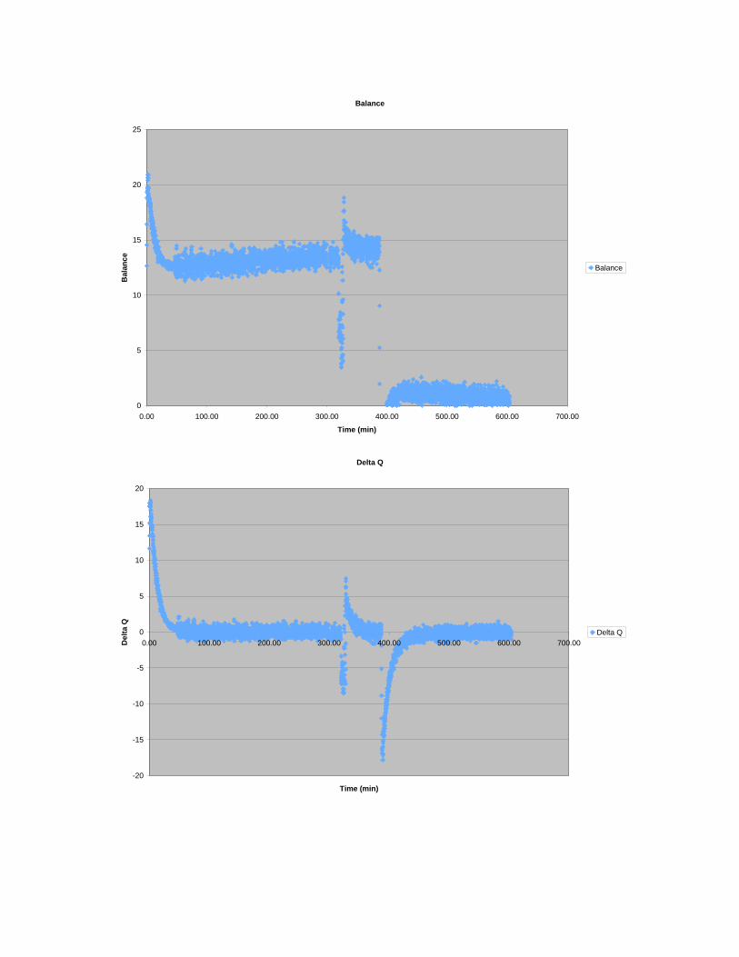
All gases behaved as expected except that the argon results were initially a surprise. Argon was chosen as a baseline to compare to CO2 because is it radiatively neutral in the IR, and therefore it would not reradiate heat inside the chamber (unlike CO2). As can be seen in both Table 2 and the figures in the Appendix however, argon not only resulted in an increase in temperature, but the increase was even higher than that seen with the addition of CO2. This is thought to be due to convection within the chamber, which played a bigger role than expected, and also because argon is a good insulator and a poor convector. Figure 5 shows the magnitude of convection occurring for each gas. In comparing the non-greenhouse gases, argon convects less than nitrogen, and thus the sphere heated up more because less heat was carried away by convection. Convection played a role in the heat transport within the chamber due to heat reradiating off of the chamber walls. The chamber was constructed with a water jacket that was meant to be filled with cold water in order to draw the heat out of the atmosphere within the chamber, and hence to cut down on any convective effects. However, due to time constraints we were unable to do any runs with the water jacket filled. Therefore, as the sphere heated up, convection began to set in within the chamber. Figure 4 shows our low pressure experiment; it can be seen that convection plays a larger role at lower atmospheric pressures because the density of the air is lower, allowing for the buoyant forces to overcome the viscous forces. Once the pressure was increased to 1 atm, the convective component of heat transfer decreased. Furthermore, heating due to the greenhouse effect increased as there was a higher concentration of greenhouse gas molecules within the chamber.

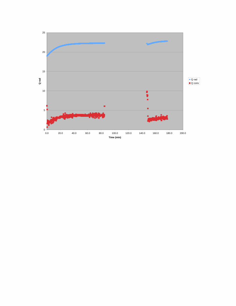
Figure 5 compares the radiative cooling to the convective cooling for the

air CO2 N Ar run. Air proved to be the best convector and the worst radiator while argon was the worst convector and the best radiator. This resulted in the ball heating up the most with an argon atmosphere because it was unable to cool itself as efficiently via convection as the other gases were. Also, argon has a low specific heat and therefore more heat was able to be transferred to the atmosphere so it heated up more. Argon has the same thermal conductivity as CO2, indicating that some other property is coming into play---probably the heat capacity.

The graphs in the Appendix show plots of temperature of each of the

thermocouples over time, change in temperature over time, heat balance over time, heat flux (energy flux) over time, and the convective and radiative heat components over time. The heat balance was calculated using the equation:

10

Balance = Q sss ppp hhh eee rrr eee+Qrad-Qwall where Qsphere = ΔTCpm (m = mass of sphere)

The heat from radiation, the walls, and convection were all calculated using the Stefan-Boltzmann Law. The heat flux was calculated using the equation:

ΔQ = Qlamp-Qsphere-Qrad+Qwall

Preliminary results indicate that there may be a relationship between the heat

capacity of a gas and how well it convects. Figure 6 shows a plot of heat capacity vs. convective cooling at 48 °C. Argon and nitrogen, the two worst convectors in our experiments, plot linearly with each other. Air, which is predominantly (~80%) nitrogen, plots slightly higher than the Ar-N line, and pure CO2 plots farther off the line, showing a departure from the Ar-N line with increasing ease of convection in the gas. Further study on the relationship between heat capacity and convective cooling within gases is needed to solidify whether or not the trend we observed in our experiments is indeed the general case.

Figure 4: Heat balance graph for the low pressure air (1 atm) run.

11

Figure 5: Comparison of radiative and convective cooling in the air CO2 N Ar run.

Figure 6: Convective cooling vs. heat capacity.

CONCLUSIONS AND FUTURE WORK

Utilizing principles of radiative equilibrium, greenhouse gas effects on the radiative forcing of the Earth, and convective cooling, Joop's World demonstrates the respective roles of carbon dioxide gas and convective cooling in affecting the energy balance of the actual Earth. Although our results do suggest a role for carbon dioxide in the re-equilibration of the aluminum/brass sphere at higher temperatures, the unanticipated influence of convective cooling in the chamber clouded our results. The

12

argon results may have been influenced by the fact that we used industrial-grade gas, and therefore it may have had slight contaminants. Had the water jacket been utilized, this would have succeeded in minimizing the role of convection, yielding results more purely and accurately indicative of the role of CO2 on global warming. Future work on Joop's World would include the use of this water jacket as well as investigation into the relationship between the heat capacity of a gas (and perhaps other properties of the gas) and its convective capacity.

Persistence in perfecting and experimenting with this and other analog Earth models is incredibly important given the state of the environment. We are currently experiencing global climate change, largely due to an accelerating influx of carbon dioxide from anthropogenic sources. A better understanding of the sensitivity of the Earth and feedback patterns is crucial for being able to effectively mitigate the causes and consequences of global warming.

APPENDIX

4/9/2008: Air->CO2, 250 W, Brass Sphere

4.9 Air then CO2 250W

0.000

10.000

20.000

30.000

40.000

50.000

60.000

70.000

0 100 200 300 400 500 600 700

Time (min)

Tem

pera

ture

(C)

Brass sphereAtmosphere

Air->CO2 250 W

-0.500

-0.400

-0.300

-0.200

-0.100

0.000

0.100

0.200

0.300

0.400

0.500

0.00 100.00 200.00 300.00 400.00 500.00 600.00 700.00

Time (min)

Del

ta T

Air->CO2

Balance

0

5

10

15

20

25

0.00 100.00 200.00 300.00 400.00 500.00 600.00 700.00

Time (min)

Bal

ance

Balance

Delta Q

-20

-15

-10

-5

0

5

10

15

20

0.00 100.00 200.00 300.00 400.00 500.00 600.00 700.00

Time (min)

Del

ta Q

Delta Q

0

5

10

15

20

25

30

35

0.00 100.00 200.00 300.00 400.00 500.00 600.00 700.00

Time (min)

Q ra

d Q radSeries2

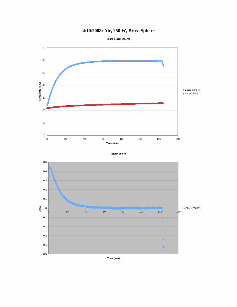
4/10/2008: Air, 250 W, Brass Sphere

4.10 blank 250W

0

10

20

30

40

50

60

70

0 20 40 60 80 100 120 140

Time (min)

Tem

pera

ture

(C)

Brass SphereAtmosphere

Blank 250 W

-0.5

-0.4

-0.3

-0.2

-0.1

0

0.1

0.2

0.3

0.4

0.5

0 20 40 60 80 100 120 140

Time (min)

Del

ta T

Blank 250 W

Balance

0

2

4

6

8

10

12

14

16

18

20

0 20 40 60 80 100 120 140

Time (min)

Bal

ance

Balance

Delta Q

-20

-15

-10

-5

0

5

10

15

20

0 20 40 60 80 100 120 140

Time (min)

Del

ta Q

Delta Q

0

5

10

15

20

25

30

35

0 20 40 60 80 100 120 140

Time (min)

Q ra

d Q radQ conv

4/14/2008: Air->CO2, 150 W, Brass Sphere

Room Air Followed by CO2, 150 W

0

5

10

15

20

25

30

35

400

3.67

7.33 11

14.7

18.3 22

25.7

29.3 33

36.7

40.3 44

47.7

51.3 55

58.7

62.3 66

69.7

73.3 77

80.7

84.3

150

154

157

161

165

168

172

176

Time (min)

Tem

pera

ture

(C)

Brass SphereAir

Air+CO2

-0.2

-0.1

0

0.1

0.2

0.0 20.0 40.0 60.0 80.0 100.0 120.0 140.0 160.0 180.0 200.0

Time (min)

Del

ta T

Air+CO2

Balance

0

1

2

3

4

5

6

7

0.0 20.0 40.0 60.0 80.0 100.0 120.0 140.0 160.0 180.0 200.0

Time (min)

Bal

ance

Balance

Delta Q

-8

-6

-4

-2

0

2

4

6

8

0.0 20.0 40.0 60.0 80.0 100.0 120.0 140.0 160.0 180.0 200.0

Tme (min)

Del

ta Q

Delta Q

0

5

10

15

20

25

0.0 20.0 40.0 60.0 80.0 100.0 120.0 140.0 160.0 180.0 200.0

Time (min)

Q ra

d Q radQ conv

4/15/2008: Argon, 250 W, Brass Sphere

Argon 250 W

0

10

20

30

40

50

60

70

800

8.83

17.7

26.5

35.3

44.2 53

61.8

70.7

79.5

88.3

97.2

106

115

124

133

141

150

159

168

177

186

194

203

212

221

230

239

247

256

265

274

Time (min)

Tem

pera

ture

(C)

Brass SphereAirWall

Delta T

-0.600

-0.400

-0.200

0.000

0.200

0.400

0.600

0.0 50.0 100.0 150.0 200.0 250.0 300.0

Time (min)

Del

ta T

Delta T

Balance

0

5

10

15

20

25

0.0 50.0 100.0 150.0 200.0 250.0 300.0

Time (min)

Bal

ance

Balance

Delta Q

-20

-15

-10

-5

0

5

10

15

20

0.0 50.0 100.0 150.0 200.0 250.0 300.0

Time (min)

Del

ta Q

Delta Q

0

5

10

15

20

25

30

35

40

0.0 50.0 100.0 150.0 200.0 250.0 300.0

Time (min)

Q ra

d Q radQ conv

4/18/2008: Argon CO2, 150 W, Brass Sphere

Argon Followed by CO2, 150 W

0

10

20

30

40

50

600

6.33

12.7 19

25.3

31.7 38

44.3

50.7 57

63.3

69.7 76

82.3

88.7 95 101

108

114

120

127

133

139

146

152

158

165

171

177

184

190

196

Time (min)

Tem

pera

ture

(C)

Brass SphereAirWall

Ar+CO2

-0.300

-0.200

-0.100

0.000

0.100

0.200

0.300

0.0 20.0 40.0 60.0 80.0 100.0 120.0 140.0 160.0 180.0 200.0

Time (min)

Del

ta T

Ar+CO2

Balance

0

1

2

3

4

5

6

7

8

9

10

11

0.0 20.0 40.0 60.0 80.0 100.0 120.0 140.0 160.0 180.0 200.0

Time (min)

Bal

ance

Balance

Delta Q

-10

-8

-6

-4

-2

0

2

4

6

8

10

0.0 20.0 40.0 60.0 80.0 100.0 120.0 140.0 160.0 180.0 200.0

Time (min)

Del

ta Q

Delta Q

0

5

10

15

20

25

30

0.0 20.0 40.0 60.0 80.0 100.0 120.0 140.0 160.0 180.0 200.0

Time (min)

Q ra

d

Q radQ conv

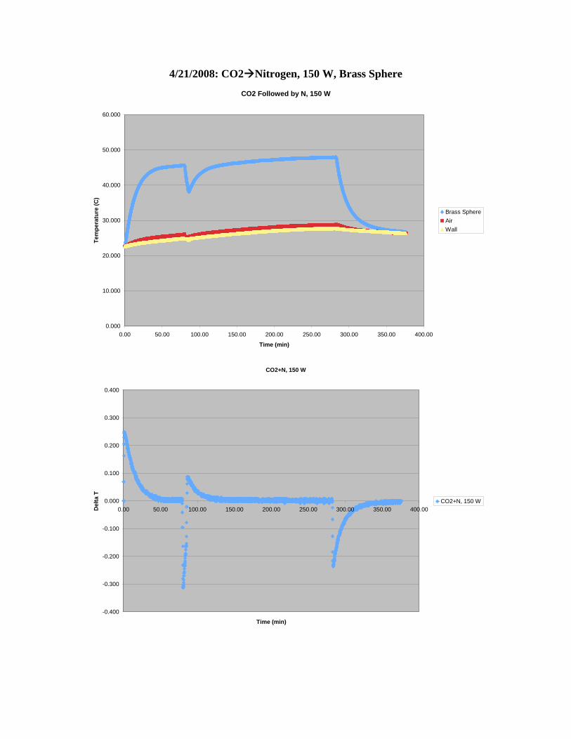
4/21/2008: CO2 Nitrogen, 150 W, Brass Sphere

CO2 Followed by N, 150 W

0.000

10.000

20.000

30.000

40.000

50.000

60.000

0.00 50.00 100.00 150.00 200.00 250.00 300.00 350.00 400.00

Time (min)

Tem

pera

ture

(C)

Brass SphereAirWall

CO2+N, 150 W

-0.400

-0.300

-0.200

-0.100

0.000

0.100

0.200

0.300

0.400

0.00 50.00 100.00 150.00 200.00 250.00 300.00 350.00 400.00

Time (min)

Del

ta T

CO2+N, 150 W

Balance

0

2

4

6

8

10

0.00 50.00 100.00 150.00 200.00 250.00 300.00 350.00 400.00

Time (min)

Bal

ance

Balance

Delta Q

-10

-8

-6

-4

-2

0

2

4

6

8

10

0.00 50.00 100.00 150.00 200.00 250.00 300.00 350.00 400.00

Time (min)

Del

ta Q

Delta Q

0

5

10

15

20

25

30

0.00 50.00 100.00 150.00 200.00 250.00 300.00 350.00 400.00

Time (min)

Q ra

d Q radQ conv

4/22/2008: Air, 150 W, Aluminum Sphere

Air, Al Sphere, 150 W

0.000

10.000

20.000

30.000

40.000

50.000

60.000

0.0 50.0 100.0 150.0 200.0 250.0 300.0

Time (min)

Tem

pera

ture

(C)

Al SphereAirWall

Air, 150 W

-0.400

-0.300

-0.200

-0.100

0.000

0.100

0.200

0.300

0.400

0.0 50.0 100.0 150.0 200.0 250.0 300.0

Time (min)

Del

ta T

Air, 150 W

Balance

0

2

4

6

8

10

12

0.0 50.0 100.0 150.0 200.0 250.0 300.0

Time (min)

Bal

ance

Balance

Delta Q

-10

-8

-6

-4

-2

0

2

4

6

8

10

0.0 50.0 100.0 150.0 200.0 250.0 300.0

Time (min)

Del

ta Q

Delta Q

0

10

20

30

40

50

60

70

0.0 50.0 100.0 150.0 200.0 250.0 300.0

Time (min)

Q ra

d Q radQ conv

4/23/2008: Air CO2 Nitrogen Argon, 150 W, Aluminum Sphere

Air Followed by CO2 Followed by Nitrogen, 150 W

0.000

10.000

20.000

30.000

40.000

50.000

60.000

0.00 200.00 400.00 600.00 800.00 1000.00 1200.00

Time (min)

Tem

pera

ture

(C)

Al SphereAirWall

Delta T

-0.500

-0.400

-0.300

-0.200

-0.100

0.000

0.100

0.200

0.300

0.400

0.500

0.00 200.00 400.00 600.00 800.00 1000.00 1200.00

Time (min)

Del

ta T

Delta T

Balance

0

2

4

6

8

10

12

0.00 200.00 400.00 600.00 800.00 1000.00 1200.00

Time (min)

Bal

ance

Balance

Delta Q

-15

-10

-5

0

5

10

15

0.00 200.00 400.00 600.00 800.00 1000.00 1200.00

Time (min)

Del

ta Q

Delta Q

0

5

10

15

20

25

30

35

0.00 200.00 400.00 600.00 800.00 1000.00 1200.00

Time (min)

Q ra

d Q radQ conv

4/24/2008: Low Pressure Air (1 atm), 150 W, Aluminum Sphere

20

25

30

35

40

45

50

55

0 50 100 150 200 250Time (min)

Tem

pera

ture

(o

C)

T sphere

low P air

air 1 atm

Light off

Delta T

-0.500

-0.400

-0.300

-0.200

-0.100

0.000

0.100

0.200

0.300

0.400

0.500

0.000 50.000 100.000 150.000 200.000 250.000

Time (min)

Del

ta T

Delta T

-4

-2

0

2

4

6

8

10

12

0 50 100 150 200 250

Time (min)

QL -

Qco

nv +

Q g

rh

balance

low P air

air 1 atm

Light off

Delta Q

-15.00

-10.00

-5.00

0.00

5.00

10.00

15.00

0.000 50.000 100.000 150.000 200.000 250.000

Time (min)

Del

ta Q

Delta Q

02468

10121416182022242628

0 50 100 150 200 250Time

Q (

*1

0)

QradQ conv

low P air

air 1 atmLight off