Joosung, Ko

Ch8. Analysis

2

outline

1. Introduction2. What do we want to analyze?3. Reachability analysis4. Structural analysis

1. Place invariants2. Transition invariants3. Automated calculation of invariants

5. Simulation1. Example the taxi company2.simulation using CPN Tools

6. Classical Petri nets Vs High level Petri nets

It is reasonable to make such a process model.

Making a process model can help us to understand it better.

A Petri-net-based process model can be used as a specification or a design of a system to be developed.

A Petri-net-based process model can also be used for the analysis of a system.

In this chapter, we study how to use Petri nets for the purpose of analysis.

1. Introduction

We can ask some questions to know about some systems.

Two question types : qualitative and quantitative questions.

If you answer, ‘yes’ or ‘no’ -> qualitative

If you answer, ‘number, frequency’ -> quantitative

There are two reasons to distinct these questions

2. What do we want to analyze?

In reachability analysis, the reachability graph of a Petri net is analyzed.

With this graph of the Petri net, we can answer a number of qualitative Questions.

By inspecting the reachability graph Of a high-level Petri net, we can gain insight into the occupation rates, efficiency, performance and costs of the modeled situation.

3. Reachability Analysis

rg1 rg2

r1 r2

go1 go2

g1 g2

or1 or2

o1 o2

x

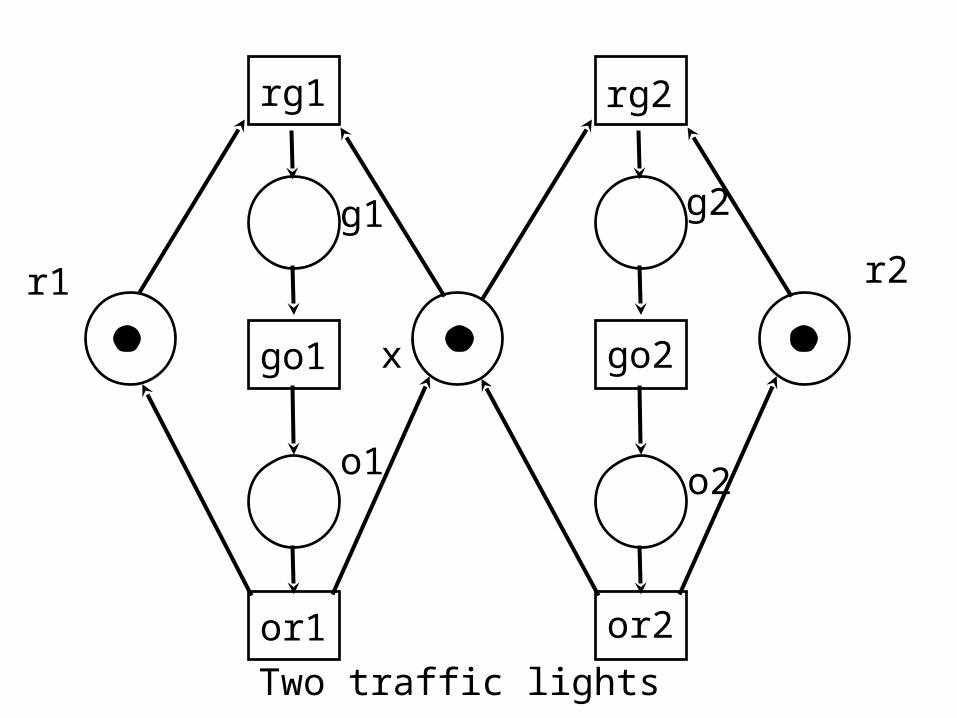
A model for two traffic lights.

4. Structural Analysis

The number of nodes in the reachability graph on the initial state.

It is difficult to use reachability analysis when you have unlimited reachable states.

start_production start_consumption

freeproducer

product

end_production

end_consumption

waitconsume

Producers and consumers

a. Place Invariants

A place invariants assigns to each place a weight, in such a way that no transition can change the weighted token sum.

A place invariant represents a kind of preservation law.man

woman

couple

marriage

divorce

A classical Petri net

freeend

docu

donewait

start change

busy

insideA business process involving a specialist

rg1 rg2

r1 r2

go1 go2

g1 g2

or1 or2

o1 o2

x

Two traffic lights

b. Transition invariants

We use transition invariants to prove that a Petri net returns to the initial state after a certain series of firings

A transition invariant assigns each transition t a weight wt in such a way that firing each transition t wt times does not change the state. The weight of a transition is not allowed to be a negative number.

A transition invariant does not indicate in which order the transition should fire. Only the number of firings per transition is fixed.

Transition invariants are the counterparts of place invariants.We can use invariants in two ways

- We can verify whether previously determined properties indeed apply.

- We can derive invariants and subsequently check which properties they represent.

man

woman

couple

marriage

divorce

p1

p2 p3

p4

winter

spring autumn

summer

A classical Petri net

The four seasons

Place and transition invariants are structural techniques, and the invariants can be checked and calculated efficiently.

We can simply describe how invariants can be computed.

It is important to note that a Petri net can be represented by a matrix having a row for each place and a column for each T.

The incidence matrix of a Petri net can be used for all kinds of analysis.

It is not difficult to calculate a basis and there are many techniques to obtain the most interesting invariants.

c. Automated calculation of invariants

The purpose of simulation is to avoid too costly or dangerous experiments.

We study the simulation in the sense of experimenting with a high-level Petri net representing processes of reality.

We can run the simulation through the reachability graph.To clarify things we need to discuss the concept “probability

distribution” since these are typically used to specify delays in a simulation model.

During the simulation all kinds of things can be measured.To determine the reliability of the measurements, the simulation

run is often divided into a number of subruns.

5. Simulation

2 4 6 8 10 duration (min)

0.1

0.2

0.3

probability

2 4 6 8 10 duration (min)

0.1

0.2

0.3

probability

A uniform distribution of probability for service durations

A negative exponential probability distribution for the time in between two arrivals

a. Example: The Taxi Company

HSHS

color Car=string

arrive Car

environment gas_station

drive_on Car

depart Car

Page main modeling the gas station and its environment

Page gas_station

fill_up

color Car = string;color Pump = until;

color TCar = Car timed;color Queue = list Car;

var c:Car;var q:Queue;

fun len(q:Queue) = if q=[] then 0

else 1+len(tl(q));

ln

arrive Car

drive_on

c

[len(q)<3] c c

c

c

put_in_queue

queueQueue

q^^[c]q

q

q

q

[]

start

()

()

()Pump

c@+uniform(2,5)

pump_free

TCar

end

outout

depart Car Cardrive_on

c::q

b. simulation using cpn tools

lnarrive

Car

drive_on

c

[len(q)<3] cc

c

c

put_in_queue

queue

Queue

q^^[c]q

q

q

q

[]

start

()

()

()

Pump

c@+discrete(2000,5000) pump_free

end

out outdepart

Car Car

drive_on

c::q

Carfill_up

Page gas_station in CPN Tools

1 1’01’0

1 1’1@01’1@0

[len(q)>=3]

counter create arrive

count_do record_depart_on drive_on

percentage

count_d

average_d

record_drive_dodepartsum_do

INT

INT Car

Car

Car

0

0

0

0

0

in

in

out

1

j+1@+round(exponential(1.0/4000.0))

i

i

(“car_”^Int.toString(i),IntInf.toInt(time()))

i+1

kc

INT(i*100)div(i+1)

INT

INTi

j

i+1i k

I div(i+1)

(cid,t)

1

1

1

1

1

1

1’01’0

1’01’0

1’01’0

1’01’0

1’01’0

1’1@01’1@0

Page environment in CPN Tools.

arrive Car

environment

gas_station

drive_on

Car

depart

Car

The top level of the simulation model

environmentgas_station

The effect of adding three extra places to the waiting space.

23

6. classical petri nets Vs high-level petri nets

The classical Petri net allows for many types of analysis and many questions are tractable

To gain insight into applicability of analysis methods to high level nets we discuss each f the three extensions and their effect on analysis- The extension with color increases the expressive power of Petri

nets considerably.- The extension with time adds a dimension to the Petri net- The extension with hierarchy allows for the construction of large

and complex models but does not complicate analysis.

color BlackToken = unit;var b:BlackToken

CS1

BlackTokenBlackToken

BlackToken

BlackToken

BlackToken

CS5

CS4

CS3

CS2

()

()

()

()()

HS

HS HS

HS

HS

philosopherleft = CS1

right = CS5

philosopherleft = CS5

right = CS4

philosopherleft = CS4

right = CS3

philosopherleft = CS3

right = CS2

philosopherleft = CS2

right = CS1

PH5

PH4 PH3

PH2

PH1

Definition of top-level page five _philosopher

25

Thank you